Business School The University of Sydney

OME WORKING PAPER SERIES

Bayesian Forecasting for Financial Risk Management,

Pre and Post the Global Financial Crisis

Richard Gerlach Business School

The University of Sydney

Cathy WS Chen Feng Chia University, Taiwan

Edward MH Lin Feng Chia University, Taiwan

Wcw Lee

Feng Chia University, Taiwan

Abstract

Value-at-Risk (VaR) forecasting via a computational Bayesian framework is considered. A range of parametric models are compared, including standard, threshold nonlinear and Markov switching GARCH specifications, plus standard and nonlinear stochastic volatility models, most considering four error probability distributions: Gaussian, Student-t, skewed-t and generalized error distribution. Adaptive Markov chain Monte Carlo methods are employed in estimation and forecasting. A portfolio of four Asia-Pacific stock markets is considered. Two forecasting periods are evaluated in light of the recent global financial crisis. Results reveal that: (i) GARCH models out-performed stochastic volatility models in almost all cases; (ii) asymmetric volatility models were clearly favoured pre-crisis; while at the 1% level during and post-crisis, for a 1 day horizon, models with skewed-t errors ranked best, while IGARCH models were favoured at the 5% level; (iii) all models forecasted VaR less accurately and anti-conservatively post-crisis.

March 2011

OME Working Paper No: 03/2011 http://www.econ.usyd.edu.au/ome/research/working_papers

Bayesian Forecasting for Financial Risk Management, Pre and

Post the Global Financial Crisis

CATHY WS CHEN1∗, RICHARD GERLACH2, EDWARD MH, LIN1, AND WCW LEE1

1Feng Chia University, Taiwan2University of Sydney Business School, Australia

ABSTRACT

Value-at-Risk (VaR) forecasting via a computational Bayesian framework is considered. Arange of parametric models are compared, including standard, threshold nonlinear and Markovswitching GARCH specifications, plus standard and nonlinear stochastic volatility models, mostconsidering four error probability distributions: Gaussian, Student-t, skewed-t and generalizederror distribution. Adaptive Markov chain Monte Carlo methods are employed in estimationand forecasting. A portfolio of four Asia-Pacific stock markets is considered. Two forecastingperiods are evaluated in light of the recent global financial crisis. Results reveal that: (i) GARCHmodels out-performed stochastic volatility models in almost all cases; (ii) asymmetric volatilitymodels were clearly favoured pre-crisis; while at the 1% level during and post-crisis, for a 1 dayhorizon, models with skewed-t errors ranked best, while IGARCH models were favoured at the5% level; (iii) all models forecasted VaR less accurately and anti-conservatively post-crisis.

KEY WORDS: EGARCH model; generalized error distribution; Markov chain Monte Carlo method;Value-at-Risk; Skewed Student-t; market risk charge; global financial crisis.

INTRODUCTION

Financial risk management has undergone much change and greater regulation in the last twentyyears following, and in many ways in response to, the major stock-market crash (“Black Monday”)

∗Correspondence to: Cathy W.S. Chen, Department of Statistics, Feng Chia University, Taichung, Taiwan. Email:

chenws@fcu.edu.tw

1

of October, 1987. Now, another major market incident, the global financial crisis (GFC) in 2008-09,has prompted calls for more and different financial regulation. In order to better control the riskof financial institutions and to protect them against large unexpected losses, the group of G-10countries agreed in 1988 to sponsor and subsequently form the original Basel Capital Accord. Inthe last two decades, however, large unexpected losses have continued to occur with regularity: e.g.in December 1994, Orange County (US) announced a loss of $1.6 billion in its’ investment portfolio;in 1995, Nick Leeson, of Barings Bank (UK), lost $1.4 billion in speculation, primarily on futurescontracts; in 1997, the Asian financial crisis began, which started in Thailand with the financialcollapse of the Thai baht; among others, and finally the very recent GFC. Financial markets andthe products traded on them are continuing to become more complicated and difficult to properlyunderstand and assess by existing risk management tools and regulations. Such methods and rulesclearly need to evolve as well.

Value-at-Risk (VaR) was pioneered in 1993, as a part of the “Weatherstone 4:15pm” dailyrisk assessment report, in the RiskMetrics model at J.P. Morgan. By 1996, amendments to theBasel Accord (Basel Accord II) allowed banks to use an ‘appropriate model’ to calculate theirVaR thresholds. Jorion (1997) defines VaR as a measure of the highest expected loss, over agiven time interval, under normal market conditions, at a given confidence level: VaR is thus aconditional quantile of the asset return loss distribution. Following Basel II, VaR has becomemore popular and is widely used in practice for risk management and capital allocation. Therecommended back-testing guideline proposed by the Basel Committee on Banking Supervision(1996) is to evaluate a one percent (1%) VaR model over a 12 month test period (250 tradingdays). VaR has been criticised for not measuring the magnitude of a loss in case of an extremeevent. As such, and following McAleer and da Veiga (2008), we also consider various criteriameasuring the loss magnitude given a violation, such as mean and maximum absolute deviation.These measures go beyond assessing violation rates and allow risk management to incorporate lossmagnitude. Further, the different measures of model performance allow financial institutions toselect different combinations of alternative risk models to forecast VaR using selection or combiningstrategies to suit their purpose.

The GFC came to the forefront of the business world and global media in September 2008,with the failure and merging of several American financial companies, e.g. the federal takeover ofFannie Mae and Freddie Mac, Lehman Brothers filing for bankruptcy after being denied supportby the Federal Reserve Bank. However, the ”credit-crunch” became apparent in January, 2008 andit has been suggested the whole GFC was pre-empted by house prices falling in June, 2007. In late2008, a number of indicators suggested that the major stock indexes were in a downward spiralglobally. Consequently, how to forecast market risk, via VaR, during such extreme periods, becomesa crucial issue in risk management and investment. To shed light on this issue, this study examines

2

a sample of four major Asia-Pacific Economic Cooperation (APEC) stock markets, being the dailystock indices: Nikkei 225 Index (Japan), HANG SENG Index (Hong Kong), the Korea Composite(KOSPI) Index; and the US S&P 500 Index. To test a range of competing models in varying marketconditions, the forecast period was split up into two segments: the first finishes at 29 February2008, well before the effects of the GFC on world markets were clear. The second validation samplestarts in August 2008 and includes the worst of the GFC period and some ”post-crisis” period aswell.

There are many approaches to forecasting VaR: these include non-parametric methods, e.g.historical simulation (using past or in-sample quantiles); semi-parametric approaches, e.g. extremevalue theory and the dynamic quantile regression CAViaR model (Engle and Manganelli, 2004); andparametric statistical approaches that fully specify model dynamics and distributional assumptionse.g. RiskMetricsTM (J.P. Morgan, 1996) and GARCH models (see Engle, 1982 and Bollerslev,1986). The aim of this paper is to compare a range of well-known, modern and fully parametriceconometric models to forecast VaR, under a Bayesian framework, before, during and after the GFC.Each model includes a specification for the volatility dynamics and most consider four specificationsfor the conditional asset return distribution: Gaussian, Student-t, generalized error distributions(GED) and the skewed Student-t of Hansen (1994). When forecasting VaR thresholds, our goal is tofind the optimal combination of volatility dynamics and error distribution in terms of the observedviolation rates and the magnitude of the deviation of violating returns, both pre and during/afterthe GFC.

The focus here is on parametric models and Monte Carlo simulation. However, many of themodels are flexible, with quite pliable error distributions and differing specifications for volatil-ity dynamics, that can capture the main empirical or stylized facts observed for financial assetreturn data: fat tails (lepto-kurtosis), volatility clustering and asymmetric volatility (Poon andGranger, 2003). We consider popular variants and extensions of the GARCH model family asfollows: RiskMetrics; symmetric GARCH; integrated GARCH (IGARCH), Engle and Bollerslev(1986); asymmetric GJR-GARCH, Glosten, Jaganathan, and Runkle (1993); asymmetric exponen-tial GARCH (EGARCH), Nelson (1991); threshold nonlinear GARCH (TGARCH), Zakoian (1994)and the Markov switching GARCH, Chen, So and Lin (2009). Further, we consider two stochasticvolatility (SV) models: the symmetric SV and the threshold nonlinear SV model of Chen, Liu andSo (2008).

Bayesian Markov chain Monte Carlo (MCMC) methods have a number of advantages in es-timation, inference and forecasting, including: (i) accounting for parameter uncertainty in bothprobabilistic and point forecasting; (ii) exact inference for finite samples; (iii) efficient and flexiblehandling of complex models and non-standard parameters, e.g. threshold and degrees of freedomparameters, which can be validly infinite; (iv) efficient and valid inference under parameter con-

3

straints. As such MCMC methods were generally used to forecast VaR thresholds for each modelin this paper. We follow Chen and So (2006) and design an efficient, adaptive MCMC samplingscheme for estimation and quantile forecasting.

Section 2 reviews the list of heteroscedastic models considered, whose details are given inan Appendix, and details the Bayesian MCMC methods used for estimation and forecasting. Theamendment to the Basel Accord was designed to reward institutions with superior risk managementsystems and suggested back-testing procedures, whereby actual (past) returns were compared withforecasts of VaR, be used to assess the quality of ‘internal’ models; we favour this approach.Seven different criteria are used to compare the forecasting performance of the various conditionalvolatility models considered in Section 4, namely: (1) violation rates; (2) mean market risk charge(MRC); (3) maximum absolute deviation (AD) of violations; (4) mean AD; (5)observed penaltyfactor; (6) the conditional coverage test; and (7) the unconditional coverage test. The last twocriteria are the standard back-testing procedures. Section 5 presents a simulation study of EGARCHwith three error distributions showing the estimation performance of the methods in Section 3.Section 6 presents the empirical results and forecasting study. Concluding remarks are given inSection 7.

MODELS

We investigate general Bayesian VaR forecasting from a list of nine popular parametric volatilitymodels with specified dynamics and four error distributions. The volatility dynamics for eachmodel are specified in detail in Appendix A. Each model has the general mean equation and errorspecification:

rt = at, at =√htεt, εt ∼ D(0, 1),

where rt is the return observation at time t; εt is a sequence of i.i.d. random variables, withmean zero (0), variance one (1) and distribution D; and ht is the conditional variance of rt. Eachmodel has a dynamic specification for ht, as in Appendix A. The common names for the modelsare: GARCH, IGARCH, RiskMetrics, GJR-GARCH, EGARCH, Threshold GARCH (TGARCH),Markov switching GARCH, stochastic volatility (SV) and threshold SV.

Four error distributions are used for the i.i.d. disturbances in each GARCH-type model εt.The choice D(0, 1) ≡ N(0, 1) is standard, and labeled as (a). The Student-t (b), GED (c), andskewed Student-t (d) distributions need to be standardized to have unit variance, as specified inAppendix A.

4

BAYESIAN APPROACH

Bayesian methods usually require the specification of a likelihood function and a prior distributionon model parameters. This section presents the general likelihood functional form for all modelsconsidered in the paper and then presents specific details for two of the nonlinear models, togetherwith details of the prior distributions employed under GED and skewed Student-t errors. We givedetails in the case of the EGARCH model with GED errors and GJR with skewed Student-t errors.Details of the likelihoods for the other models can either be deduced from the model forms above,or found in the papers referenced above.

Let Θ denote the full parameter vector for any of the combinations of model and error distri-bution considered. The conditional likelihood can be written as:

L(r|Θ) =n∏t=1

1√htpε

(rt√ht

), (1)

where ht is given by the relevant volatility equation and pε (·) is the relevant error density functionfor εt.

Exponential GARCH model and priorLet Θ denote the vector (α1, α2, γ, β, λ). The conditional likelihood for the EGARCH-GED errormodel is thus:

L(r|Θ) =

[λ

2σΓ( 1λ)

]n n∏t=1

1√ht

exp

{−

n∑t=1

∣∣∣∣ rt√htσ

∣∣∣∣λ}, (2)

where r = (r1, . . . , rn) and σ = [Γ( 1λ)/Γ( 3

λ)]0.5.

The prior distribution is chosen to be reasonably uninformative so that the likelihood dominatesinference. The prior for α=(α1, α2, γ) is chosen as a Gaussian: α ∼ N(0,V ), with the diagonalvariance-covariance matrix (V ) chosen to have ‘large’ diagonal elements; e.g. 1. This prior makessense since these parameters are unrestricted, but empirical studies show they are usually estimatedto be close to, though still significantly different from, 0. This prior is reasonably diffuse in theregion close to 0, and well beyond, where empirical parameter estimates usually lie.

The parameter β is restricted for stationarity, via |β1| < 1. The prior for this parameteris chosen to be uniform over this region. For the shape parameter λ, Vrontos, Dellaportas, andPolitis (2000) set a log-normal prior with mean 1.04 · 1022 and variance 2.93 · 1087. Such a choiceseems excessively diffuse. Instead we employed a half-normal distribution, λ ∼ Nc(0, 1), which is astandard normal truncated to lie on the positive real line, i.e. λ ∈ (0,∞).

5

The prior for (α, β, λ) is assumed independent in the three groupings, so that:

p(α, β, λ) ∝ exp{−12

(α)TV −1(α)− 12λ2} · I(β ∈ (−1, 1)). (3)

GJR-GARCH model and priorThe GJR-GARCH model specification is given in (16), here considered with a skewed Student-terror distribution. The likelihood for the GJR-GARCH-st model is thus:

L (r|α, ν, η) =

n∏t=1

bc√ht

[1 + 1

ht(ν−2)

(brt+a

√ht

1−η

)2]−(ν+1)

2I1,rt +

[1 + 1

ht(ν−2)

(brt+a

√ht

1+η

)2]−(ν+1)

2I2,rt

where α = (α,0α1, β1, γ1)′; I1,rt = I(rt <

−a√ht

b

), and I2rt = 1− I1rt .

Again priors are set that are mostly uninformative over the restricted parameter region in (17).That is, the prior for α is flat over (17); while for the degrees of freedom, we re-parameterize viaτ = ν−1 and set the prior for τ as U(0, 0.25). This ensures that ν > 4 and that the first fourmoments of the error distribution are finite. Finally, we set a flat prior over η ∈ (−1, 1).

These settings for the EGARCH and GJR-GARCH models are indicative of the prior settingsused for the other models. Further details for the other models may be found in Chen and So(2006). The joint posterior distribution for each model is formed by multiplying the likelihood bythe joint prior for that model. The posteriors for each model are not in the form of a standardor known distribution in the parameters. As such we turn to computational MCMC methods toobtain estimation and inference from each posterior.

MCMC methodsMCMC methods have proven successful for nonlinear time series in general, e.g. see Chen and Lee(1995); Vrontos, Dellaportas, and Politis (2000); Chen and So (2006) and others. MCMC methodssimulate iteratively from the conditional posteriors of groups of model parameters. We discussgeneral details here, as well as some specific details for the EGARCH model and for the GED andskewed Student-t distributions. This is the first time a skewed Student-t error GARCH-type modelhas been estimated by MCMC methods in the literature, to the best of our knowledge.

The typical parameter groupings are: α, plus any thresholds or parameters in the error dis-tribution. For the EGARCH-GED model, parameter groupings are: (i) (α, β) and (ii) λ. For theTGARCH model with skewed Student-t errors, parameter groupings would be: α, w, d, ν, η. Theposterior for each parameter group, conditional upon the other parameters, is formed separately bymultiplying the likelihood (1) by the prior for that parameter group. None of these conditional pos-terior distributions are in a standard form to facilitate direct simulation from, for all models here,

6

as such we turn to Metropolis-Hastings type methods; see Metropolis et al. (1953) and Hastings(1970).

To speed convergence and to allow optimal mixing properties, we employ an adaptive MCMCalgorithm that combines a random walk Metropolis (RW-M) and an independent kernel (IK-)MHalgorithm, following Chen and So (2006). For the burn-in period, a Gaussian proposal distributionis employed in a RW-M algorithm. The variance-covariance matrix of this proposal is subsequentlytuned to achieve optimal acceptance rates, as in Gelman et al. (1996). After the burn-in period,the sample mean vector and sample variance-covariance matrix of the iterates are formed. Theseare employed in the sampling period as the proposal mean and proposal variance-covariance matrixfor a Gaussian proposal in an IK-MH algorithm. Such an adaptive proposal updating procedurewill be highly efficient, as long as the burn-in period has ‘covered’ the posterior distribution. SeeChen and So (2006) for more details. We extensively examine trace plots and autocorrelationfunction (ACF) plots from multiple runs of the MCMC sampler, for each model parameter andfrom different starting positions, to confirm convergence and infer adequate coverage. Details forthe sampling scheme for the MS-GARCH model can be found in Chen, So and Lin (2009).

FORECASTING RETURNS, VOLATILITY AND VaR

Forecasting utilizing MCMC methods can efficiently incorporate parameter uncertainty in a straight-forward fashion. The steps below outline how to generate l-step-ahead l-day return and volatilityforecasts, from the models and error distributions considered, using forecast origin t = n. Thesesteps are performed at each MCMC iteration in the MCMC sampling period, using the currentiterate (j) for each model’s full parameter set, denoted Θ[j]:

1. Calculate hn+1 using the in-sample data up until time t = n, r, the relevant volatility equationfrom (1)-(9) and Θ[j]. Set i = 1.

2. Simulation step: draw εn+i ∼ D(0, 1) where D is one of the four standardized error distribu-tions. Calculate rn+i = an+i =

√hn+iεn+i.

3. Evaluation step: evaluate hn+i+1 using hn+i, the simulated an+i from 2., the in-sample datar, the relevant volatility equation from (1)-(9) and Θ[j].

4. Set i = i+ 1 and go to 2.

7

The process is continued up to the simulation of εn+l and calculation of rn+l. These steps gen-erate one realization from the joint distribution of rn+1, . . . , rn+l|r,Θ[j]. Repeating this process forj = 1, . . . , J while also simulating Θ[j] from the relevant model’s posterior distribution, numericallyintegrates out Θ and obtains a Monte Carlo sample from the forecast distribution rn+1, . . . , rn+l|r.Summing each l-day vector of returns, i.e.

∑li=1 rn+i gives one sample from the l-day forecast

return distribution, conditional upon r, as required.

The main purpose of this paper is to forecast VaR thresholds. VaR at level α can be definedas:

Pr (∆V (l) ≤ −VaR) = α, (4)

where ∆V (l) is the change in the asset value over l time periods. As standard, we considerα = 0.05, 0.01.

A one-step-ahead VaR is simply the α-level quantile of the l = 1-step conditional distributionrn+1|Fn ∼ D(0, hn+1). Here hn+1 is given by one of the models (1)-(7), and D is the relevant errordistribution in (a)-(d). This predictive distribution is estimated via the MCMC simulation usingthe steps above: i.e. the MCMC samples give Θ[j], h

[j]n+1 for iterates j = M + 1, . . . , N , which is

the MCMC sampling period. Then, the quantile VaR is given by:

VaR[j]n+1 = −

[D−1α (Θ[j])

√h

[j]n+1

], (5)

where D−1 is the inverse CDF for the distribution D. For errors (b), (c) and (d) the CDF dependson some unknown parameters, which explains the notation. Then, the final forecasted one-step-ahead VaR is the Monte Carlo posterior mean estimate:

VaRn+1 =1

N −M

N∑j=N−M

VaR[j]n+1, (6)

The l-day VaR is the α-level quantile of the l-day return distribution An(l) =∑li=1 rn+i|Fn.

The steps detailed above simulate a Monte Carlo sample A[j]n (l) = a

[j]n+1 + ... + a

[j]n+l; j = 1, . . . , J

from this forecast distribution. The l-day VaR is:

VaRn(l) = −G−1α (An(l)|Fn). (7)

where in general the l-day CDF G is not D. As such, we take the empirical or sample quantileestimate from the Monte Carlo sample A[j]

n (l); j = 1, . . . , J at the required level α to estimateVaRn(l).

One exception is under the RiskMetricsTM model. Here, the square root of time rule is impliedby the model so that:

VaRn(l) =√l ×VaRn+1. (8)

8

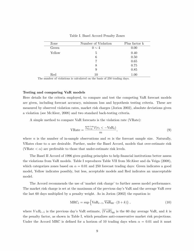
Table I. Basel Accord Penalty Zones

Zone Number of Violation Plus factor kGreen 0 ∼ 4 0.00Yellow 5 0.40

6 0.507 0.658 0.759 0.85

Red 10 1.00The number of violations is calculated on the basis of 250 trading days.

Testing and comparing VaR modelsHere details for the criteria employed, to compare and test the competing VaR forecast modelsare given, including forecast accuracy, minimum loss and hypothesis testing criteria. These aremeasured by observed violation rates, market risk charges (Jorion 2002), absolute deviations givena violation (see McAleer, 2008) and two standard back-testing criteria.

A simple method to compare VaR forecasts is the violation rate (VRate):

VRate =Σn+mt=n I(rt < −VaRt)

m, (9)

where n is the number of in-sample observations and m is the forecast sample size. Naturally,VRates close to α are desirable. Further, under the Basel Accord, models that over-estimate risk(VRate < α) are preferable to those that under-estimate risk levels.

The Basel II Accord of 1996 gives guiding principles to help financial institutions better assessthe violations from VaR models. Table I reproduces Table VII from McAleer and da Veiga (2008),which categorizes zones based on α = 0.01 and 250 forecast trading days: Green indicates a goodmodel, Yellow indicates possibly, but less, acceptable models and Red indicates an unacceptablemodel.

The Accord recommends the use of ‘market risk charge’ to further assess model performance.The market risk charge is set at the maximum of the previous day’s VaR and the average VaR overthe last 60 days multiplied by a penalty weight. As in Jorion (2002) the equation is:

MRCt = sup{

VaRt−1,VaR60 · (3 + k)} , (10)

where V aRt−1 is the previous day’s VaR estimate, (V aR)60 is the 60 day average VaR, and k isthe penalty factor, as shown in Table I, which penalizes anti-conservative market risk projections.Under the Accord MRC is defined for a horizon of 10 trading days when α = 0.01 and it must

9

be based on at least a year of historical in-sample data. Models with lower MRCs are consideredbetter in terms of risk measurement.

The magnitude of violating returns, not just their VRate, is also important, i.e. the expectedloss given a violation. Thus, measures of loss magnitude are also considered here. The AD ofviolating returns, considered by McAleer and da Veiga (2008), is:

ADt = |rt − (−(V aR)t)| , (11)

defined only when rt is a violation. The mean and maximum AD are calculated here to comparecompeting VaR models: models with lower mean and/or maximum ADs are preferred.

SOME MONTE CARLO RESULTS

Simulation studies are performed to examine the effectiveness of the MCMC sampling scheme. Theerror distributions were chosen as: (i) the GED with parameters λ = 1, 1.5 and λ = 2 and (ii) theskewed Student-t St(7, η) with η = −0.05,−0.5,−0.99. Specifically, the models we consider are:

Model 1: The true model is an EGARCH-GED model.

rt = at,

at =√htεt, εt

i.i.d.∼ GED(0, λ),

ln(ht) = −0.2 + 0.2|at−1| − 0.26at−1√

ht−1+ 0.93 ln(ht−1),

where εt follows the standardized GED(0, λ) distribution. The form of Model 2 is the same asModel 1, but the distribution of εt is set as the skewed Student-t, St(7, η).

For each model we simulated 100 replicated data sets, repeating this over sample sizes ofn=2,000 and 4,000. For each dataset we used a total of 20,000 MCMC iterations, with a burn-inperiod of M=8,000 iterations. We choose initial values for the EGARCH parameters as α = 0 andtail-thickness parameter λ = 0.1 in Model 1, while the degrees of freedom ν was set at 200 andη was set as 0 in Model 2. These are generally quite poor starting values and our results are notsensitive to different choices.

Table II about here

Table II shows the estimation results for the simulated datasets, including true parametervalues, means, standard deviations, 2.5 and 97.5 percentiles for the 100 posterior mean estimates,

10

over the replicated data sets, at each sample size. All of the means of the estimates are close totheir respective true values, with reasonable standard errors that reduce with increasing samplesize. For the GED errors, λ = 2 causes no problem at all, despite the low prior weight attached tothis value from the half-standard normal prior. For the skewed Student-t error model, η = −0.99also causes minimal problems, despite being close to the boundary value of η = −0.99, the bias inestimation being practically negligible.

EMPIRICAL STUDY

For the empirical study, an asset portfolio of four major Asia-Pacific Economic Cooperation (APEC)stock markets is considered. Four daily stock price indices, including three major Asian markets:the Nikkei 225 Index (Japan), HANG SENG Index (Hong Kong) and the Korea Composite (KOSPI)Index; as well as the US S&P 500 Index. The data were obtained from Datastream Internationalover a 12-year time period, from October 1, 1997 to December 30, 2009.

For each market, the returns are the logarithmic difference of the daily price index, as apercentage:

rt = (log(Pt)− log(Pt−1))× 100,

where Pt is the closing index value on day t. We consider a single equally weighted portfolio ofthese assets, with return:

rp,t =4∑i=1

wi × ri,t,

where rp,t is the portfolio return at time t, ri,t is the return of asset i = 1, . . . , 4 at time t andwi = 0.25 is the weight on each market’s return. This portfolio return series is now analyzed.

To examine the performance of the models under highly varied market conditions, this studyexamines two distinct forecasting periods. The first complete data set is divided into two: anin-sample period of October 1, 1997 to July 8, 2005, and a forecast or validation period, containingthe m = 588 observations: July 9, 2005 to February 29, 2008. This is a period before the effects ofthe GFC hit the markets.

To examine how the models perform during the 2008-09 GFC, and evaluate how the crisisaffects risk management, a second time span in considered: a learning period of October 4, 2000to July 31, 2008, of similar sample size to the pre-crisis learning sample, and a 2nd validation or

11

forecast period of 316 trading days: August 1, 2008 to December 30, 2009. This covers the worsteffects of the GFC on markets.

A rolling window approach is used to produce 1 and 10-day forecasts of the 1% VaR and 1-dayforecasts of the 5% VaR thresholds in both forecast samples. The models were: RiskMetricsTM , sixGARCH-type models: IGARCH, GARCH, TGARCH, GJR-GARCH, EGARCH, and MS-GARCH,respectively, where the GARCH-type models all employed each of the four error distributions; andtwo SV models: the symmetric SV and THSV models, specified in equations (22) − (23), withGaussian and Student-t distributions only. The threshold value r = 0 and the delay lag d = 1were used, in accord with general assumptions in the literature. Thus, 29 risk models in totalare considered. The first n return observations, i.e. each in-sample period, were initially used toestimate each model and then to forecast the returns rn+1, . . . , rn+l, as detailed in Section 5, forl = 1, 10. The in-sample period was then rolled forward by one observation, so that it rangedfrom r2 to rn+1, whereby the returns rn+2, . . . , rn+l+1 are forecasted. This roll-forward process wasrepeated until each day in the forecast sample was forecast. To strike a balance between estimationefficiency and a feasible number of forecasts, a rolling window size of approximately n = 1700observations was chosen, leaving m = 588 observations to be forecasted in the first sample period,and m = 316 in the second.

For illustration, time series plots of the one-day-ahead forecasts of ht based on the GJR-GARCH-t, GJR-GARCH-st, EGARCH-GED, and EGARCH-t models are presented in Figure 1.This illustrates the similarity among well-specified volatility models, but also highlights that dif-ferences can occur, especially in periods of high volatility.

Back-testingTwo back-testing criteria (unconditional, UC and conditional coverage, CC) for examining theaccuracy of the models for VaR are employed. The simplest method tests the hypothesis thatthe VRate is equal to α. Kupiec (1995) examines whether VaR estimates, on average, providecorrect UC of the lower α percent tails of the forecasted return distributions. Christoffersen (1998)developed a CC test that simultaneously examines unconditional coverage and independence ofviolations: it is a joint test that the true violation rate equals α and that the violations areindependent.

Several criteria are used to compare the forecasting performance of the various conditionalvolatility models considered, namely: (1) VRate; (2) mean MRC; (3) maximum AD of violations;(4) mean AD; (5)observed penalty factor; (6) the CC test; and (7) the UC test.

1 day forecasting results: pre-crisis periodWe first discuss the pre-crisis forecast period: July 9, 2005 to February 29, 2008. Table VII showsp-values for the UC and CC tests for the one-day VaR forecast models at the 99% confidence level

12

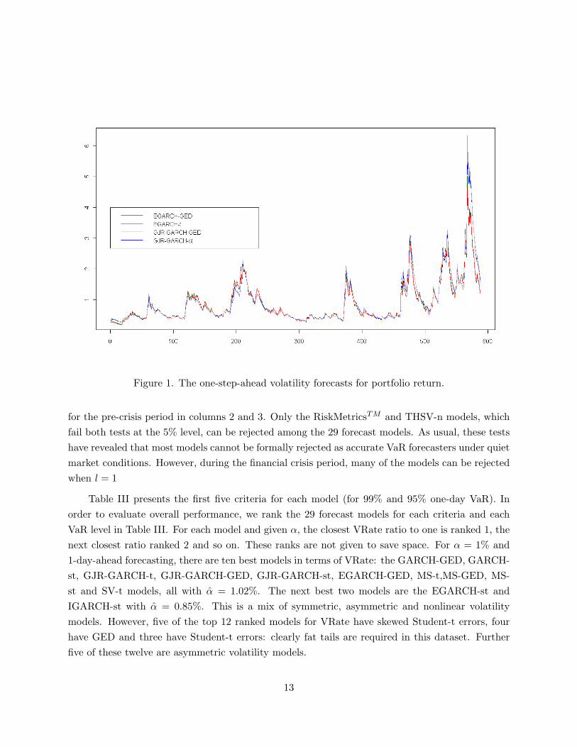
Figure 1. The one-step-ahead volatility forecasts for portfolio return.

for the pre-crisis period in columns 2 and 3. Only the RiskMetricsTM and THSV-n models, whichfail both tests at the 5% level, can be rejected among the 29 forecast models. As usual, these testshave revealed that most models cannot be formally rejected as accurate VaR forecasters under quietmarket conditions. However, during the financial crisis period, many of the models can be rejectedwhen l = 1

Table III presents the first five criteria for each model (for 99% and 95% one-day VaR). Inorder to evaluate overall performance, we rank the 29 forecast models for each criteria and eachVaR level in Table III. For each model and given α, the closest VRate ratio to one is ranked 1, thenext closest ratio ranked 2 and so on. These ranks are not given to save space. For α = 1% and1-day-ahead forecasting, there are ten best models in terms of VRate: the GARCH-GED, GARCH-st, GJR-GARCH-t, GJR-GARCH-GED, GJR-GARCH-st, EGARCH-GED, MS-t,MS-GED, MS-st and SV-t models, all with α = 1.02%. The next best two models are the EGARCH-st andIGARCH-st with α = 0.85%. This is a mix of symmetric, asymmetric and nonlinear volatilitymodels. However, five of the top 12 ranked models for VRate have skewed Student-t errors, fourhave GED and three have Student-t errors: clearly fat tails are required in this dataset. Furtherfive of these twelve are asymmetric volatility models.

13

In terms of mean market risk charge (MRC), 6 of the top 7 ranked models had Gaussian errors.Since the Gaussian error models all under-estimated risk levels at 1%, it is not surprising they showthe smallest MRC, which depends on the average VaR over 60 days. Under the maximum and meanADs the asymmetric models dominate the top rankings, with 6 of the top 9 ranked models, for ADMax, and 10 of the top 12 for AD Mean. Further, under AD fat-tailed errors occupy the top 8rankings for AD max and 9 of the top 12 for AD mean.

The overall best models are the GJR-GARCH models: with GED, Student-t, skewed Student-t and Gaussian errors. The four EGARCH models are next best overall took. Thus asymmetricvolatility models did best here, while among these models, those with fat-tailed errors did best,especially those with GED and skewed-t errors. The RiskMetricsTM model performed the worst intwo of the five measures, including VRate (with a large 2.72%), had the largest penalty factor andwas overall close to the THSV-n model in performance.

It is clear that volatility asymmetry is highly important at α = 0.01 and l = 1 while the choiceof error distribution was less important prior to the GFC. Further, GARCH-type models mostlyfinished well ahead of the SV-type models; only the SV-t was competitive with any GARCH modelhere, with the other three SV models ranking close to the bottom across all measures. The resultssuggest that, prior to the crisis, at the 1% quantile of the distribution, the asymmetric volatilityeffect, is strong and important and capturing this feature allowed better predictability for extremereturns in this portfolio, far more so than the shape of the (error) distribution and any associatedproperties like skewness, kurtosis, etc did.

Table III about here

For α = 5%, the overall best models are the GARCH-st, GJR-GARCH-st model (which ranked1st for both mean and max AD), the EGARCH-st and the IGARCH-st models, so the first fouroverall best models had skewed Student-t errors. The RiskMetricsTM model ranked last for VRateand close to last overall, the THSV models overall being marginally worse. Clearly, skewed errorsare highly important at α = 0.05 when l = 1 and a GARCH or GJR specification seems bestunder that choice. The results suggest that at the 5% quantile of the distribution, the shape of the(error) distribution, especially whether it is skewed, is very important when l = 1, and capturingthis feature allowed better predictability for the 5th percentile of returns in this portfolio. Theasymmetric volatility effect was also still important, but was secondary in this respect.

Figure 2 exhibits one-day ahead VaR forecasts and realized returns for the best four modelsconsidered, in the forecast sample, at α = 0.01. The four GJR-GARCH models’ VaR forecastthresholds are violated six to eight times in 588 returns. In summary for one-day ahead VaRforecasting in this sample, asymmetric models have dominated the overall rankings at α = 0.01,

14

while still featuring prominently at α = 0.05; while skewed Student-t errors were only stronglyfavoured when α = 0.05. The best combined choice of model was the GJR-GARCH with skewedStudent-t errors. The RiskMetricsTM , symmetric SV with Gaussian errors and both THSV modelstended to be at or near the bottom of the rankings for this sample of data under these measures.

1 day forecasting results: GFC periodWe now discuss the results at the 1% risk level for 1-day-ahead forecasting in the period thatcontains the GFC: August 1, 2008 to December 30, 2009. Table VII shows p-values for the UC, CCtests at the 99% confidence level for this period in columns 4 and 5. The RiskMetricsTM , GJR-GARCH-n, EGARCH-n, EGARCH-t, EGARCH-GED and all four SV-type models are rejectedby both tests at the 5% level. Further, models rejected by UC only include the GJR-GARCH-t,GJR-GARCH-GED and MS-n. These models are excluded from the discussion to follow.

Results for the other five criteria are shown in Table IV. For models surviving the UC, CCtests, there are nine best models in terms of VRate: the GARCH-t, GARCH-GED, GARCH-st, IGARCH-t, IGARCH-GED, IGARCH-st, MS-t, MS-GED and MS-t, all with α = 1.58%, i.e.risk under-estimated by 58%, with 5 observed violations compared to the expected 3.16; all modelsunder-estimated risk levels in this GFC dominated period. This is a mix of symmetric and nonlinearvolatility models, with asymmetric volatility and Gaussian error distributions not represented. Sixof the nine models have non-stationary volatility equations, indicating the enormous and quicklychanging effects from the GFC.

In terms of MRC, again MS, GARCH and EGARCH models occupied the top 7 ranks, againall with fat-tailed errors. Under the maximum AD the rejected EGARCH model takes the firstthree rankings, while four of the top 6 ranked models have skewed-t errors; for both max AD andmean AD IGARCH-st ranks best among surviving models, followed by GJR-st and GARCH-st:clearly skewed errors are important for ADmax and mean. The overall best models are GARCH-stmodel and IGARCH-st. Most of the best overall models have skewed-t errors, while models withGaussian errors all did poorly on most criteria. The RiskMetricsTM model ranked worst of allthe GARCH-type models, but ahead of the four SV models that again occupied the bottom, nowincluding the SV-t.

Clearly, during and following the GFC, a skewed error distribution with fat tails is very im-portant to capture risk dynamics and level, at 1%, at a one day horizon. Gaussian errors were leastfavoured, while nonlinear and symmetric volatility models were favoured over asymmetric ones.

For α = 5%, again all models under-estimated risk, s.t. α > 5%. The overall best modelsare the IGARCH-st (top ranked in VRate, with 5.38%), GJR-GARCH-st, IGARCH-GED andIGARCH-n models. The RiskMetricsTM model did much better here ranking 6th overall andequal 4th for violation rate. The SV models, however, again performed the worst of all models.

15

The results suggest that at the 5% quantile of the return distribution in the GFC period, theshape of the (error) distribution, and whether asymmetry is included, are not the most importantaspects when l = 1. Instead, non-stationary IGARCH models seem to do best, even including theRiskMetrics approach.

At both 1, 5% levels during the crisis IGARCH models performed comparably among the bestduring and after the GFC. At the 1% level fat tails and skewness were important in the errordistribution; while at 5% the error distribution was not that important.

Table IV about here

10 day forecasting results: pre-crisisWhen considering 10-day VaR, it is not appropriate here to conduct either the UC or CC tests sincewe considered over-lapping ten-day returns. We would expect these returns to cluster, as wouldour VaR forecasts and hence the observed violations. Violations should thus not be independentwhen over-lapping returns are used, nor should the iid assumption in the UC test be valid.

The empirical results of the 10-day VaR forecasting (l = 10) for the pre-crisis forecast periodare in Table V. The amendments to Basel II allow banks freedom to use ‘appropriate’ internalmodels to measure their exposure to market risks, requiring this to be summarized as a 1% Value-at-Risk over a 10 day horizon. Thus only α = 1% was considered. Here, the stand-out bestmodel in terms of VRate was the EGARCH-n, with α = 1.04%, followed by the EGARCH-st withα = 1.21%. The GJR-GARCH models ranked poorly here with 1.55% (skewed Student-t error)and 1.73% for the other error distributions, while the RiskMetricsTM was worst with 2.94%. Interms of mean MRC the TGARCH-t model ranked best, with the GJR models all ranking in thebottom places. For both maximum and mean ADs, the EGARCH and GJR-GARCH obtained allthe top 8 rankings, with EGARCH best. The overall top ranked models were the four EGARCHmodels, with EGARCH-n and EGARCH-st the best two. The RiskMetricsTM model was again thelast ranked model overall and regarding VRate.

In summary for ten-day return VaR forecasting, at α = 0.01, in this pre-crisis sample, asym-metric models have dominated, with the E-GARCH dominating the high rankings; the EGARCH-nranking first or second for 3 forecast risk measures. The RiskMetricsTM model was again at thebottom of the rankings for this sample of data under these measures.

10 day forecasting results: GFC periodThe 10-day VaR forecasting results and rankings for the 2nd forecast sample period are given inTable VI. Here, all models under-estimate risk levels substantially. The best models in terms ofVRate were the IGARCH-st and the GJR-GARCH-n, each having α ≈ 3, indicating that observed

16

(a)

(b)

Figure 2. VaR forecasts for the period before the global financial crisis (a) 1-day-ahead and (b) andten-day ahead VaR forecasts at 1% level.

17

VRate was 3 times higher than nominal. Oevrall, the IGARCH-st, IGARCH-GED and IGARCH-n were best overall. In terms of mean MRC the EGARCH models ranked best, followed by theTGARCH models, with the IGARCH and RM models ranking in the bottom places. For bothmaximum and mean ADs, the IGARCH and GARCH obtained most of the top 10 rankings. Theoverall best models were the IGARCH-st, IGARCH-GED and IGARCH-n models. The SV-typeand RiskMetricsTM model were the last ranked models overall.

In summary for ten-day return VaR forecasting, at α = 0.01, in this GFC dominated sample,all the model struggled and substantially under-estimate risk levels. The IGARCH model didcomparatively better, but no model does well at all. The RiskMetricsTM model was again at thebottom of the rankings for this sample of data under these measures.

Tables V-VI about here

For these two forecast periods, it seems that completely different models have dominated forl = 1, 10 and during pre-crisis and crisis periods. No overall single model can be recommended inboth quiet and highly volatile market conditions. Instead, the best model depends on the forecasthorizon l and quantile level α and overall market conditions. For one (l = 1) and ten (l = 10)day VaR forecasting pre-crisis, modeling asymmetry is very important, but in different ways. Forone-day forecasting the GJR-GARCH with skewed Student-t errors did best overall, while theGJR models as a group occupied the top 4 placings at α = 0.01 and 3 of the top 6 at α = 0.05.The EGARCH models tended to rank just below the GJR models for l = 1. The choice of errordistribution for l = 1 seemed slightly less important than ensuring that asymmetry was effectivelycaptured, though skewed Student-t error models dominated at α = 0.05. However, during the GFCperiod, asymmetry was far less important; instead employing a skewed error distribution with fattails was critical to capturing risk dynamics and level, while non-stationary IGARCH and MSmodels did comparatively best, though all models did under-estimate risk levels during this period.

For ten-day VaR forecasting, in the pre-crisis period the EGARCH model with Gaussian errorsdid best for α = 0.01, followed by the other three EGARCH models. In this case Gaussian errorsseemed to be quite adequate and to even do better than the fat-tailed distributions; this result mightbe influenced by the aggregation of 10 single day returns being closer to normality, as expectedstatistically, than a single day’s return distribution. We further note that the simplest and mostparsimonious asymmetric models (i.e. not the TGARCH) dominated at both l = 1 and l = 10days.

In the GFC forecast period, however, all models significantly under-estimated risk levels ata 10-day horizon and no model could be recommended as accurate. To better understand thisoutcome, the bottom panel of Figure 2 exhibits ten-day ahead VaR forecasts and realized returns

18

for the best four models during the pre-crisis period, which are EGARCH with various errors. TheVaR forecasts violate the thresholds six to eight times from 579 forecasts in the pre-crisis period:the violations are few and spread out without clustering. Figure 3 shows the equivalent results inthe GFC-dominated 2nd forecast period, for the best two models. Now, there is a large numberof clustered violations all occurring in quick succession in October, 2008, at the start of the mostdramatic effects of the GFC on daily returns. The dates for the clustered violations are the 9th,10th, 14th, 15th, 20th, 21st and 23rd October, 2008. Clearly and logically, the 1-day ahead VaRforecasts can adjust to the global financial crisis effects and subsequent extreme returns far morequickly (9 days more quickly in fact) than the 10-day ahead VaR forecasts. This result is clearlyheavily influenced by our use of 10 day periods that overlap by 9 days; the 10 day forecasting resultsresults may have been better if we analysed non-overlapping 10 day periods.

This study considered a range of well-known, modern and popular, fully parametric econo-metric models to estimate and forecast VaR under a Bayesian framework. Each model includes aspecification for the volatility dynamics and further, most models consider four specifications forthe asset return error distribution. We observed from the empirical study that a conservative riskmodel often yielded a lower violation rate and correspondingly higher mean market risk charge andthat different models were required depending on length of forecast horizon and quantile level, aswell as for different market conditions. Also, while the 1-day forecasts, especially for non-stationarymodels, adapted reasonably well to the recent GFC, no model could be recommended for the recentGFC dominated period for 10-day ahead forecasting. McAleer, Jimenez-Martin, and Perez-Amaral(2009) illustrate two useful variations to the standard mechanism for choosing forecasts, namely:(i) combining different forecast models for each period, such as a daily model that forecasts thesupremum or infinum value for the VaR; (ii) alternatively, select a single model to forecast VaR,and then modify the daily forecast, depending on the recent history of violations under the BaselII Accord. Our study can provide valuable information for Deposit-taking Institutions (ADIs) tohelp choose risk models for predicting their VaR. Further, ADIs could employ combinations ofprominent models based on our findings as a management strategy for forecasting VaR.

Table VII about here

CONCLUSIONS

This paper assesses the possibility of general Bayesian forecasting for carrying out one to tenday ahead VaR forecasting across a range of competing parametric heteroskedastic models. Nine

19

popular volatility models are compared, most with four separate error distributions. For one andten-day VaR forecasting, the well-known RiskMetricsTM model ranked last in most measures andwas rejected in all cases by the diagnostic tests. No model did consistently well across the differentforecast horizons or quantile levels or market conditions. For one day ahead forecasting prior tothe financial crisis, the GJR-GARCH with skewed Student-t errors ranked best, followed by otherasymmetric volatility models. Volatility asymmetry is most important to capture, with skewederrors also prominent, especially at α = 0.05. During and after the crisis, asymmetry is notimportant, instead skewness and fat tails dominate at the 1% level, with non-stationary modelsdoing best at 5%. For ten-day ahead forecasting prior to the crisis, the EGARCH models had thebest performance, with volatility asymmetry again an important feature, while normality seemedthe best choice of error distribution. In both 1 and 10 day forecasting, all models under-estimatedrisk levels during the crisis, in fact all 10-day forecasting models were rejected for risk coverageduring and after the crisis. Further, generally, GARCH models dominated the SV models in forecastperformance. We observed from the empirical study that a conservative risk model often yieldeda lower violation rate and correspondingly higher mean market risk charge. Therefore, we suggestemploying combinations of prominent models as a management strategy for forecasting VaRs. Wewill focus on the Bayesian method helping to forecast the VaR under different investment strategiesin the future.

Acknowledgement

We thank Professor Ruey S. Tsay and the anonymous referees for their insightful commentsthat helped improve the paper. Cathy Chen is supported by National Science Council (NSC) ofTaiwan grant NSC96-2118-M-035-002-MY3.

Appendix AThe nine models considered are now given in detail:

1. Symmetric GARCHBollerslev (1986) introduced a parsimonious extension to Engle’s ARCH model:

ht = α0 +p∑i=1

αia2t−i +

q∑j=1

βjht−j . (12)

Positivity and stationary dynamics are ensured via the standard restrictions:

α0 > 0; αi ≥ 0, βi ≥ 0 andp∑i=1

αi +q∑i=1

βi < 1. (13)

20

Based on Bollerslev, Chou and Kroner (1992) we set p = q = 1. The unknown parametersare: α = (α0, α1, β1), plus any unknown parameters in D.

2. IGARCH:The IGARCH model of Engle and Bollerslev (1986) is a special case of a GARCH(1,1) withα1 + β1 = 1, i.e.:

ht = α0 + α1a2t−1 + (1− α1)ht−1, (14)

where it is common to enforce α0 ≥ 0 and 0 < α1 < 1. The volatility dynamics here are akinto those of a random walk.

3. RiskMetricsRiskMetricsTM was developed by J.P. Morgan (1996), specifically for VaR calculation and isapparently still a popular method. It is a special case of the IGARCH, where α0 = 0, andis thus an exponentially weighted moving average (EWMA) of squared shocks; further therestriction D(0, 1) ≡ N(0, 1) is used. The model form is:

ht = δht−1 + (1− δ)a2t−1, (15)

where a decay factor of 0.94 is recommended by J.P. Morgan for computing daily volatility.

4. GJR-GARCHThe GJR-GARCH model by Glosten, Jaganathan, and Runkle (1993) captures asymmetricvolatility via an indicator term in the GARCH equation:

ht = α0 +p∑i=1

(αi + γiS−t−i)a

2t−i +

q∑j=1

βjht−j (16)

where S−t−i ={

1 if at−i ≤ 0,0 if at−i > 0,

Stationarity and positive volatility are ensured via:

α0 > 0, αi, βi ≥ 0,p∑i=1

αi + γi ≥ 0 andp∑i=1

αi +q∑i=1

βi + 0.5p∑i=1

γi < 1. (17)

The usual asymmetric volatility effect, i.e. falling markets increase volatility, implies thatnegative shocks at time t lead to a larger rate of increase in conditional volatility, of αi + γi

at time t+ 1 (assuming γi > 0), whereas the positive shocks at time t lead to an increase inrate of conditional volatility of αi at time t+ 1.

21

5. Exponential GARCHNelson (1991) proposed the first asymmetric volatility model, to capture asymmetric volatil-ity: EGARCH. The general EGARCH(p,q) form is:

ln(ht) = α0 +p∑i=1

αi

(|at−i|+ γiat−i√

ht−i

)+

q∑j=1

βi ln(ht−j), (18)

where again we consider p = q = 1. Here the logarithm of volatility is modeled, allowing theusual positivity restrictions on GARCH parameters to be relaxed. We expect the asymmetriceffect γ1 < 0, so that εt−1 < 0 increases the volatility ht, where εt−1 = at−1/

√ht−1, but did

not enforce this. For stationary dynamics (see Nelson, 1991) it is natural to assume |β1| < 1.The original specification of this model used the GED for the distribution of εt.

6. Threshold GARCHA standard deviation TGARCH model was first proposed by Zakoian (1994). Instead, weconsider the dynamic variance TGARCH specification:

ht =

{α

(1)0 + Σp

i=1α(1)i a2

t−i + Σqj=1β

(1)j ht−j rt−d ≤ w

α(2)0 + Σp

i=1α(2)i a2

t−i + Σqj=1β

(2)j ht−j rt−d > w,

(19)

where d is threshold lag and w is the threshold value. Here each parameter can change inresponse to lagged returns, at unknown lag d. We again set p = q = 1. The unknown modelparameters are (α(1)

0 , α(1)1 , β

(1)1 , α(2)

0 , α(2)1 , β

(2)1 ,w, d).

7. Markov switching GARCH modelsGray (1996) and Tsay (2005) proposed simple two-state Markov switching models, with dif-ferent risk premium and different GARCH dynamics in each regime. Chen, So and Lin (2009)proposed the double Markov switching GARCH model, where here we focus on the volatilityonly. The Markov switching GARCH (MS-GARCH) is specified as:

ht = α(st+1)0 + Σp

i=1α(st+1)i a2

t−i + Σqj=1β

(st+1)j ht−j , (20)

where st is an unobserved discrete Markov process indicator. A two-regime model is employed,with p = q = 1, and a Markov transition matrix P = p(i,j), where:

p(i,j) = Pr(st = j|st−1 = i) i, j = 1, 2.

The unknown parameters are (α(1)0 , α

(1)1 , β

(1)1 , α(2)

0 , α(2)1 , β

(2)1 , p1,1, p2,2), state vector s, plus

any parameters in D.

8. Stochastic volatility modelsSV models are considered as an alternative approach to GARCH-type processes. Here, volatil-ity has a specific source of randomness and is thus stochastic, as proposed by Taylor (1982,

22

1986). The discrete-time symmetric SV model is:

at =√htεt, log ht+1 = α0 + α1 log ht + ut, (21)

where ut is a Gaussian innovation with zero mean and variance σ2u. We restrict |α1| < 1 for

stationarity.

9. Threshold SV modelsThere are quite a few papers presenting or considering a nonlinear SV model framework: e.g.So, Li and Lam (2002) presented the threshold SV (THSV) model to describe both meanand volatility asymmetry, while Chen, Liu and So (2008) generalized the THSV model andincorporated a heavy-tailed error distribution, plus estimation of the unobserved thresholdvalue and time delay parameter. We consider nonlinear SV models in asymmetric volatilitybut without a mean equation. Therefore the THSV model is:

at =√htεt, log ht+1 = (α0 + β0st) + (α1 + β1st)log ht + ut, (22)

where the state variable st is defined by

st ={

0 if rt−d < r,1 if rt−d ≥ r,

with the delay d and threshold value r.

Apart from the Riskmetrics model, all the GARCH-type volatility models are estimated underthe following distributional assumptions of the unconditional shocks (a) standard normal, (b) theStudent-t, (c) GED, and (d) skewed Student-t distributions, where:

(c) Generalised Error Distribution: The density function for εt a standardized GED withscale parameter σ is:

pε(εt) =λ

2σΓ(1/λ)exp

{−∣∣∣∣εtσ∣∣∣∣λ}, (23)

where σ = [Γ( 1λ)/Γ( 3

λ)]0.5. λ ∈ (0,∞) is the tail-behaviour determining parameter. Whenλ > 2, the distribution has thinner tails than the normal; when λ = 2, it is exactly a normaldistribution with mean 0 and standard error σ; while for λ < 2, the distribution has excesskurtosis relative to the normal. For real asset return data, we expect λ < 2.

(d) Skewed Student-t Distribution: To allow for skewness in the shape of the conditionalreturn density, the skewed Student-t distribution was defined by Hansen (1994) as:

pε(εt|ν, η) =

bc

[1 + 1

ν−2

(bεt+a1−η

)2]−(ν+1)/2

if εt < −ab

bc

[1 + 1

ν−2

(bεt+a1+η

)2]−(ν+1)/2

if εt ≥ −ab

(24)

23

where degrees of freedom ν and skewness parameter η satisfy 2 < ν < ∞, and −1 < η < 1,respectively. The constants a, b, and c are fixed as:

a = 4ηc(ν−2ν−1

); b2 = 1 + 3η2 − a2; c =

Γ

(ν+1

2

)√π(ν−2)Γ(ν2 )

.

This distribution already has zero mean and unit variance. We use the notation St(ν, η). Thestandardized Student-t distribution is a special case of this skewed Student-t, when η = 0.The Gaussian is thus the limiting distribution as ν →∞, also when η = 0.

The symmetric and skewed Student-t and the GED all allow fat-tailed error distributions, comparedto the Gaussian, while each contains the Gaussian as a special case.

References

Basel Committee on Banking Supervision. 1996. Supervisory Framework for the Use of ‘Backtest-ing’ in Conjunction With the Internal Models Approach to Market Risk Capital Requirements.BIS: Basel.

Bollerslev T. 1986. Generalized autoregressive conditional heteroskedasticity. Journal of Econo-metrics 31: 307-327.

Bollerslev T., Chou RY., Kroner KP. 1992. ARCH modeling in finance: A review of the theoryand empirical evidence. Journal of Econometrics 52: 5-59.

Christoffersen P. 1998. Evaluating interval forecasts. International Economic Review 39: 841-862.

Chen CWS, Lee JC. 1995. Bayesian inference of threshold autoregressive models.Journal of TimeSeries Analysis 16: 483-492.

Chen CWS, Liu FC, So MKP. 2008. Heavy-tailed distributed threshold stochastic volatility modelsin financial time series. Australian & New Zealand Journal of Statistics 50: 29-51.

Chen CWS, So MKP. 2006. On a threshold heteroscedastic model. International Journal ofForecasting 22: 73-89.

Chen CWS, So MKP, Lin EMH. 2009. Volatility forecasting with double Markov switchingGARCH models. Journal of Forecasting 28: 681-697.

Engle RF. 1982. Autoregressive conditional heteroskedasticity with estimates of the variance ofUnited Kingdom inflations. Econometrica 50: 987-1007.

24

Engle RF, Bollerslev T. 1986. Modelling the Persistence of Conditional Vari- ances. EconometricReviews 5: 1-50.

Engle RF, Manganelli S. 2004. CAViaR: Conditional autoregressive value at risk by regressionquantiles. Journal of Business and Economic Statistic 22: 367- 381.

Glosten LR, Jagannathan R, Runkle DE. 1993. On the relation between the expected value andthe volatility of the nominal excess return on stock. Journal of Finance 48: 1779-1801.

Gelman A, Roberts GO, Gilks WR. 1996. Efficient Metropolis jumping rules. In Bayesian Statis-tics 5, Bernardo JM, Berger JO, Dawid AP, Smith, AFM (eds). Oxford University Press:Oxford; 599-607.

Gray SF. 1996. Modeling the conditional distribution of interest rates as a regime-switchingprocess. Journal of Financial Economics 42: 27-62.

Hansen BE. 1994. Autoregressive conditional density estimation. International Economic Review35: 705-730.

Hastings WK. 1970. Monte-Carlo sampling methods using Markov chains and their applica-tions.Biometrika 57: 97-109.

Jorion P. 1997. Value at Risk: The New Benchmark for Controlling Market Risk. McGraw-Hill:New York.

Jorion P. 2002. Fallacies about the Effects of Market Risk Management Systems. Journal of Risk5: 75-96.

Kupiec PH. 1995. Techniques for verifying the accuracy of risk measurement models. The Journalof Derivatives 3: 73-84.

McAleer M. 2008. Forecasting Value-At-Risk with a Parsimonious Portfolio Spillover GARCH(PS-GARCH) Model. Journal of Forecasting 27: 1-19.

McAleer M., da Veiga, B. 2008. Single-index and portfolio models for forecasting value-at-riskthresholds. Journal of Forecasting 27: 217-235.

McAleer M, Jimenez-Martin JA, and Perez-Amaral T (2009) Has the Basel II Accord encouragedrisk management during the 2008-09 financial crisis? Available at SSRN: http://ssrn.com/abstract=1397239

Metropolis N, Rosenbluth AW, Rosenbluth MN, Teller E. 1953. Equations of state calculationsby fast computing machines.Journal of Chemical Physics 21: 1087-1091.

25

Nelson DB. 1991. Conditional heteroscedasticity in asset returns: A new approach. Econometrica59: 347-370.

Poon SH, Granger CWJ. 2003. Forecasting volatility in financial markets: A review. Journal ofEconomic Literature 41: 478-539.

So MKP, Li WK, Lam K. 2002. A threshold stochastic volatility model. Journal of Forecasting21: 473-500.

RiskmetricsTM . 1996. J. P. Morgan Technical Document (4th edn). J. P. Morgan: New York.

Taylor SJ. 1982. Financial returns modelled by the product of two stochastic processes, a studyof daily sugar prices 1961-1979. Time Series Analysis: Theory and Practice 1. Anderson OD(ed.). North-Holland: Amsterdam, 203-226.

Taylor SJ. 1986. Modelling Financial Time Series. Wiley: New York.

Tsay RS. 2005. Analysis of Financial Time Series (2nd edn). Wiley: New York.

Vrontos ID, Dellaportas P, Politis DN. 2000. Full Bayesian Inference for GARCH and EGARCHModels . Journal of Business & Economic Statistics 18: 187-198.

Zakoian JM. 1994. Threshold heteroskedastic models.Journal of Economic Dynamics and Control18: 931-955.

Authors’ biographies:

Cathy W.S. Chen is a Distinguished Professor in the Department of Statistics, Feng ChiaUniversity, Taiwan. Her research interests include modeling and forecasting of financial timeseries, market volatility study, diagnosis and model comparison for time series models, andstatistical methods in epidemiology. She has published papers, among others, in the Journalof Business & Economic Statistics, International Journal of Forecasting, Journal of the Royalof Statistical Society Series C, Computational Statistics and Data Analysis, QuantitativeFinance, AIDS, and Emerging Infectious Diseases etc.

Richard Gerlach is Associate Professor in the Discipline of Operations Management and Econo-metrics, University of Sydney, Australia. His research interests lie mainly in financial econo-metrics and time series. His methodological work has concerned developing computationallyintensive Bayesian methods for inference, diagnosis and model comparison for time series

26

models; with recent focus on nonlinear threshold heteroskedastic models and volatility, aswell as VaR, forecasting.

Edward M.H. Lin holds a PhD degree from the Department of Statistics at Feng Chia University,Taiwan. His research interests include financial time series analysis, forecasting, Bayesianinference.

Wayne C.W. Lee holds a master degree from the Department of Statistics at Feng Chia Uni-versity, Taiwan.

Authors’ addresses:Cathy W.S. Chen, Edward M. H. Lin, and Wayne C.W. Lee, Department of Statistics,Feng Chia University, Taiwan.

Richard Gerlach, Discipline of Operations Management and Econometrics, University of Sydney,Australia.

27

(a)

(b)

Figure 3. VaR forecasts for the global financial crisis period (a) 1-day-ahead and (b) and ten-dayahead VaR forecasts at 1% level.

28

Table II. Summary statistics for parameter estimates from 100 simulated data sets from theEGARCH(1,1) model.

n = 2000 n = 4000True Mean Std Lower Upper Mean Std Lower Upper

GEDα0 -0.20 -0.232 0.043 -0.322 -0.158 -0.210 0.028 -0.269 -0.158α1 0.20 0.220 0.038 0.151 0.299 0.204 0.026 0.155 0.259γ -0.26 -0.259 0.121 -0.504 -0.038 -0.269 0.085 -0.441 -0.110β 0.93 0.907 0.028 0.844 0.952 0.922 0.017 0.885 0.951λ 1.00 1.003 0.042 0.924 1.087 1.001 0.029 0.944 1.059

GEDα0 -0.20 -0.226 0.038 -0.307 -0.157 -0.213 0.024 -0.263 -0.169α1 0.20 0.213 0.035 0.150 0.285 0.208 0.023 0.165 0.255γ -0.26 -0.273 0.103 -0.482 -0.084 -0.260 0.067 -0.391 -0.136β 0.93 0.905 0.027 0.844 0.949 0.920 0.015 0.888 0.947λ 1.50 1.505 0.069 1.374 1.645 1.496 0.049 1.403 1.593

GEDα0 -0.20 -0.222 0.034 -0.294 -0.161 -0.204 0.023 -0.251 -0.162α1 0.20 0.212 0.032 0.154 0.279 0.200 0.022 0.158 0.245γ -0.26 -0.262 0.090 -0.448 -0.097 -0.277 0.065 -0.409 -0.154β 0.93 0.909 0.023 0.856 0.947 0.923 0.014 0.892 0.948λ 2.00 2.015 0.101 1.823 2.221 2.001 0.071 1.866 2.143tα0 -0.20 -0.227 0.040 -0.311 -0.156 -0.211 0.026 -0.264 -0.163α1 0.20 0.212 0.036 0.147 0.287 0.206 0.025 0.160 0.256γ -0.26 -0.252 0.109 -0.474 -0.049 -0.270 0.071 -0.412 -0.140β 0.93 0.901 0.030 0.834 0.948 0.920 0.016 0.885 0.948ν 7.00 7.231 1.180 5.386 9.974 7.304 0.815 5.928 9.117stα0 -0.20 -0.225 0.040 -0.309 -0.155 -0.211 0.026 -0.264 -0.164α1 0.20 0.215 0.037 0.148 0.291 0.207 0.025 0.160 0.257γ -0.26 -0.273 0.112 -0.502 -0.065 -0.279 0.077 -0.438 -0.136β 0.93 0.909 0.026 0.850 0.952 0.921 0.016 0.887 0.948ν 7.00 7.073 1.101 5.326 9.621 7.194 0.784 5.859 8.923η -0.05 -0.047 0.030 -0.106 0.012 -0.051 0.021 -0.093 -0.009stα0 -0.20 -0.208 0.028 -0.266 -0.158 -0.202 0.019 -0.240 -0.167α1 0.20 0.205 0.029 0.153 0.266 0.200 0.020 0.164 0.240γ -0.26 -0.276 0.105 -0.490 -0.088 -0.281 0.073 -0.431 -0.147β 0.93 0.923 0.016 0.889 0.949 0.926 0.010 0.905 0.945ν 7.00 7.245 1.173 5.417 9.955 7.151 0.780 5.831 8.883η -0.50 -0.500 0.027 -0.551 -0.446 -0.498 0.019 -0.534 -0.460stα0 -0.20 -0.201 0.006 -0.213 -0.190 -0.200 0.004 -0.208 -0.194α1 0.20 0.200 0.007 0.188 0.213 0.200 0.004 0.192 0.209γ -0.26 -0.259 0.022 -0.301 -0.214 -0.259 0.014 -0.287 -0.232β 0.93 0.930 0.003 0.924 0.935 0.930 0.002 0.927 0.933ν 7.00 7.441 0.843 6.185 9.247 7.184 0.524 6.366 8.220η -0.99 -0.980 0.006 -0.988 -0.965 -0.985 0.003 -0.989 -0.977

(1): t and st refer to Student-t and skewed Student-t errors, respectively.29

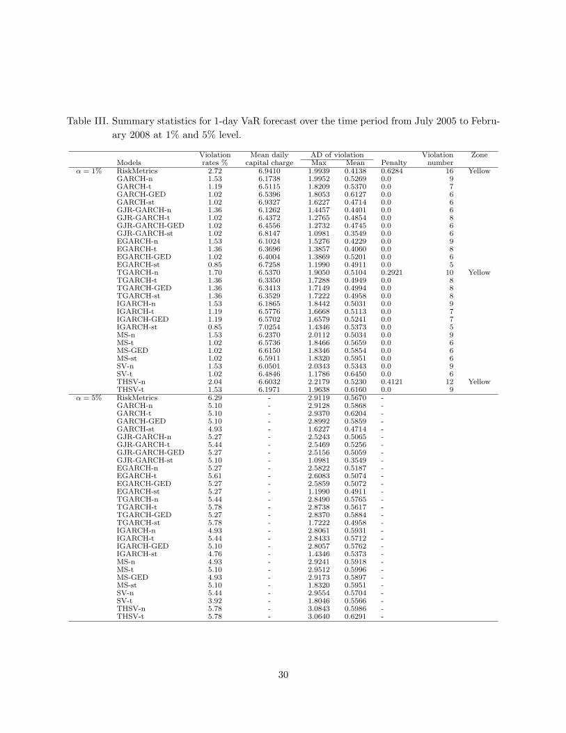
Table III. Summary statistics for 1-day VaR forecast over the time period from July 2005 to Febru-ary 2008 at 1% and 5% level.

Violation Mean daily AD of violation Violation ZoneModels rates % capital charge Max Mean Penalty number

α = 1% RiskMetrics 2.72 6.9410 1.9939 0.4138 0.6284 16 YellowGARCH-n 1.53 6.1738 1.9952 0.5269 0.0 9GARCH-t 1.19 6.5115 1.8209 0.5370 0.0 7GARCH-GED 1.02 6.5396 1.8053 0.6127 0.0 6GARCH-st 1.02 6.9327 1.6227 0.4714 0.0 6GJR-GARCH-n 1.36 6.1262 1.4457 0.4401 0.0 6GJR-GARCH-t 1.02 6.4372 1.2765 0.4854 0.0 8GJR-GARCH-GED 1.02 6.4556 1.2732 0.4745 0.0 6GJR-GARCH-st 1.02 6.8147 1.0981 0.3549 0.0 6EGARCH-n 1.53 6.1024 1.5276 0.4229 0.0 9EGARCH-t 1.36 6.3696 1.3857 0.4060 0.0 8EGARCH-GED 1.02 6.4004 1.3869 0.5201 0.0 6EGARCH-st 0.85 6.7258 1.1990 0.4911 0.0 5TGARCH-n 1.70 6.5370 1.9050 0.5104 0.2921 10 YellowTGARCH-t 1.36 6.3350 1.7288 0.4949 0.0 8TGARCH-GED 1.36 6.3413 1.7149 0.4994 0.0 8TGARCH-st 1.36 6.3529 1.7222 0.4958 0.0 8IGARCH-n 1.53 6.1865 1.8442 0.5031 0.0 9IGARCH-t 1.19 6.5776 1.6668 0.5113 0.0 7IGARCH-GED 1.19 6.5702 1.6579 0.5241 0.0 7IGARCH-st 0.85 7.0254 1.4346 0.5373 0.0 5MS-n 1.53 6.2370 2.0112 0.5034 0.0 9MS-t 1.02 6.5736 1.8466 0.5659 0.0 6MS-GED 1.02 6.6150 1.8346 0.5854 0.0 6MS-st 1.02 6.5911 1.8320 0.5951 0.0 6SV-n 1.53 6.0501 2.0343 0.5343 0.0 9SV-t 1.02 6.4846 1.1786 0.6450 0.0 6THSV-n 2.04 6.6032 2.2179 0.5230 0.4121 12 YellowTHSV-t 1.53 6.1971 1.9638 0.6160 0.0 9

α = 5% RiskMetrics 6.29 - 2.9119 0.5670 -GARCH-n 5.10 - 2.9128 0.5868 -GARCH-t 5.10 - 2.9370 0.6204 -GARCH-GED 5.10 - 2.8992 0.5859 -GARCH-st 4.93 - 1.6227 0.4714 -GJR-GARCH-n 5.27 - 2.5243 0.5065 -GJR-GARCH-t 5.44 - 2.5469 0.5256 -GJR-GARCH-GED 5.27 - 2.5156 0.5059 -GJR-GARCH-st 5.10 - 1.0981 0.3549 -EGARCH-n 5.27 - 2.5822 0.5187 -EGARCH-t 5.61 - 2.6083 0.5074 -EGARCH-GED 5.27 - 2.5859 0.5072 -EGARCH-st 5.27 - 1.1990 0.4911 -TGARCH-n 5.44 - 2.8490 0.5765 -TGARCH-t 5.78 - 2.8738 0.5617 -TGARCH-GED 5.27 - 2.8370 0.5884 -TGARCH-st 5.78 - 1.7222 0.4958 -IGARCH-n 4.93 - 2.8061 0.5931 -IGARCH-t 5.44 - 2.8433 0.5712 -IGARCH-GED 5.10 - 2.8057 0.5762 -IGARCH-st 4.76 - 1.4346 0.5373 -MS-n 4.93 - 2.9241 0.5918 -MS-t 5.10 - 2.9512 0.5996 -MS-GED 4.93 - 2.9173 0.5897 -MS-st 5.10 - 1.8320 0.5951 -SV-n 5.44 - 2.9554 0.5704 -SV-t 3.92 - 1.8046 0.5566 -THSV-n 5.78 - 3.0843 0.5986 -THSV-t 5.78 - 3.0640 0.6291 -

30

Table IV. Summary statistics for 1-day VaR forecast over the time period from August 2008 toDecember 2009 at 1% and 5% levels.

Violation Mean daily AD of violation Violation ZoneModels rates % capital charge Max Mean Penalty number

α = 1% RiskMetrics 2.85 16.0731 1.8785 0.6485 0.6662 9 YellowGARCH-n 2.22 14.3194 1.8719 0.7963 0.4701 7 YellowGARCH-t 1.58 13.0971 1.7594 0.9461 0.0 5 GreenGARCH-GED 1.58 13.0876 1.7702 0.9300 0.0 5 GreenGARCH-st 1.58 13.9422 1.5949 0.7281 0.0 5 GreenGJR-GARCH-n 3.16 14.8051 1.8134 0.6631 0.7580 10 YellowGJR-GARCH-t 2.53 14.7487 1.7184 0.6935 0.5706 8 YellowGJR-GARCH-GED 2.53 14.7377 1.7316 0.6800 0.5706 8 YellowGJR-GARCH-st 1.90 14.7298 1.5661 0.7063 0.3632 6 YellowEGARCH-n 4.11 14.5129 1.6121 0.5983 1.0 13 RedEGARCH-t 2.53 13.6267 1.4990 0.8194 0.5706 8 YellowEGARCH-GED 2.53 13.5988 1.5195 0.8017 0.5706 8 YellowEGARCH-st 2.22 13.9888 1.3186 0.7026 0.4701 7 YellowTGARCH-n 1.90 13.8305 1.8613 0.9585 0.3632 6 YellowTGARCH-t 1.90 14.6257 1.7547 0.7708 0.3632 6 YellowTGARCH-GED 1.90 14.6817 1.7878 0.7561 0.3632 6 YellowTGARCH-st 1.90 14.6806 1.7476 0.7621 0.3632 6 YellowIGARCH-n 1.90 14.4787 1.8534 0.8203 0.3632 6 YellowIGARCH-t 1.58 13.7040 1.7249 0.8046 0.0 5 GreenIGARCH-GED 1.58 13.6782 1.7460 0.7743 0.0 5 GreenIGARCH-st 1.58 14.7171 1.5414 0.5613 0.0 5 GreenMS-n 2.53 14.5145 1.8755 0.7306 0.5706 8 YellowMS-t 1.58 12.8460 1.7673 0.9710 0.0 5 GreenMS-GED 1.58 12.8570 1.7756 0.9538 0.0 5 GreenMS-st 1.58 12.9057 1.7617 0.9552 0.0 5 GreenSV-n 3.80 15.3247 1.8177 0.7905 1.0 12 RedSV-t 3.80 15.5351 1.8859 0.7766 1.0 12 RedTHSV-n 4.11 15.0285 1.9473 0.7461 1.0 13 RedTHSV-t 2.85 14.8220 1.9787 0.9578 0.6662 9 Yellow

α = 5% RiskMetrics 5.70 - 2.8836 1.1481 - 18GARCH-n 6.33 - 2.5240 1.0811 - 20GARCH-t 6.65 - 2.6710 1.0637 - 21GARCH-GED 6.33 - 2.5601 1.0685 - 20GARCH-st 6.01 - 2.5288 1.0490 - 19GJR-GARCH-n 6.65 - 2.3643 0.9913 - 21GJR-GARCH-t 6.65 - 2.3694 1.0054 - 21GJR-GARCH-GED 6.65 - 2.3588 0.9705 - 21GJR-GARCH-st 5.70 - 2.2991 1.0628 - 18EGARCH-n 7.91 - 2.6377 1.1202 - 25EGARCH-t 7.59 - 2.7201 1.1769 - 24EGARCH-GED 7.28 - 2.6604 1.1973 - 23EGARCH-st 6.96 - 2.6315 1.1924 - 22TGARCH-n 6.33 - 2.4742 1.1005 - 20TGARCH-t 6.33 - 2.6080 1.1314 - 20TGARCH-GED 6.33 - 2.5451 1.0833 - 20TGARCH-st 6.33 - 2.5871 1.1215 - 20IGARCH-n 5.70 - 2.3926 1.0611 - 18IGARCH-t 5.70 - 2.5165 1.1056 - 18IGARCH-GED 5.70 - 2.3844 1.0458 - 18IGARCH-st 5.38 - 2.3541 1.0231 - 17MS-n 6.33 - 2.5323 1.1190 - 20MS-t 6.65 - 2.6741 1.1023 - 21MS-GED 6.33 - 2.5654 1.1149 - 20MS-st 6.33 - 2.6500 1.1438 - 20SV-n 6.96 - 3.4082 1.3281 - 22SV-t 7.28 - 3.4188 1.3105 - 23THSV-n 7.59 - 3.3565 1.2375 - 24THSV-t 6.65 - 3.5129 1.4970 - 21

31

Table V. Summary statistics for 10-day VaR forecast over the time period from July 2005 to Febru-ary 2008 at 1% level.

Violation Mean Max Mean ViolationModels rates % MRC AD AD Penalty number

α = 1% RiskMetrics 2.94 23.8549 2.8712 1.3516 1.0 17GARCH-n 1.55 20.5372 3.1377 1.3509 0.0 9GARCH-t 1.73 22.6950 2.1331 0.9699 0.3018 10GARCH-GED 1.38 20.6476 2.6871 1.2621 0.0 8GARCH-st 1.73 22.7209 3.0982 1.2371 0.3018 10GJR-GARCH-n 1.73 24.4863 1.7257 0.7946 0.3018 10GJR-GARCH-t 1.73 24.3045 1.7436 0.6610 0.3018 10GJR-GARCH-GED 1.73 24.5265 1.5587 0.7595 0.3018 10GJR-GARCH-st 1.55 22.9909 1.5799 0.7104 0.0 9EGARCH-n 1.04 22.8345 1.0846 0.6005 0.0 6EGARCH-t 1.38 22.4090 1.1944 0.6784 0.0 8EGARCH-GED 1.38 22.6314 1.4140 0.6635 0.0 8EGARCH-st 1.21 22.9848 1.0897 0.5954 0.0 7TGARCH-n 2.07 22.2895 3.1077 1.1523 0.4228 12TGARCH-t 1.55 19.9576 2.9191 1.3728 0.0 9TGARCH-GED 1.90 22.2917 2.8059 1.1400 0.3636 11TGARCH-st 1.73 22.0230 2.8814 1.2719 0.3018 10IGARCH-n 1.90 23.1623 2.3457 1.0436 0.3636 11IGARCH-t 1.55 20.8814 1.9460 1.1676 0.0 9IGARCH-GED 1.38 20.7364 2.3458 1.3886 0.0 8IGARCH-st 1.38 21.9034 1.7871 1.0428 0.0 8MS-n 1.38 20.9498 2.5762 1.1561 0.0 8MS-t 1.55 20.9517 3.4019 1.1469 0.0 9MS-GED 1.38 21.1400 2.9161 1.1839 0.0 8MS-st 1.38 21.0313 2.6669 1.1512 0.0 8SV-n 1.55 21.4229 2.2366 0.8763 0.0 9SV-t 1.55 21.1760 6.2874 1.8754 0.0 9THSV-n 1.73 21.9426 2.4967 1.1147 0.3018 10THSV-t 2.07 22.4779 2.0721 0.9318 0.4228 12

(1): Ranking is based on the rank sum - min(rank) +1.

32

Table VI. Summary statistics for 10-day VaR forecast over the time period from August 2008 toDecember 2009 at 1% level.

Violation Mean Max Mean ViolationModels rates % MRC AD AD Penalty number

α = 1% RiskMetrics 4.56 56.4562 14.3576 5.9010 1.0 14GARCH-n 4.56 55.7485 13.5591 4.2880 1.0 14GARCH-t 3.91 56.3347 13.9064 5.0868 1.0 12GARCH-GED 4.23 56.4016 12.7615 4.5084 1.0 13GARCH-st 4.23 56.7473 13.0827 4.4584 1.0 13GJR-GARCH-n 2.93 53.5776 14.3099 5.4996 0.6908 9GJR-GARCH-t 3.26 56.2045 14.0292 5.4960 0.7842 10GJR-GARCH-GED 3.26 55.7099 14.2936 5.4079 0.7842 10GJR-GARCH-st 3.26 57.4997 13.0436 4.9579 0.7842 10EGARCH-n 3.91 51.9789 15.7044 6.7057 1.0 12EGARCH-t 4.23 52.5195 15.5255 6.2060 1.0 13EGARCH-GED 4.23 52.1868 16.2898 6.2683 1.0 13EGARCH-st 4.23 53.7964 15.2139 6.0211 1.0 13TGARCH-n 3.58 55.3203 13.6326 5.2069 1.0 11TGARCH-t 3.58 56.4543 12.9199 5.0923 1.0 11TGARCH-GED 3.58 56.1658 13.2295 5.0925 1.0 11TGARCH-st 4.23 56.3909 13.1970 4.5041 1.0 13IGARCH-n 3.26 56.1735 11.4370 4.4251 0.7842 10IGARCH-t 3.58 59.8153 13.1993 4.4120 1.0 11IGARCH-GED 3.26 56.6589 12.9220 5.0194 0.7842 10IGARCH-st 2.93 58.6673 11.6024 4.3722 0.6908 9MS-n 4.23 54.7926 13.3201 4.5804 1.0 13MS-t 4.23 55.1816 13.1817 4.6993 1.0 13MS-GED 4.89 54.9963 14.0789 4.0494 1.0 15MS-st 3.58 55.4635 13.1504 5.4578 1.0 11SV-n 4.89 54.4702 14.5713 5.7060 1.0 15SV-t 4.23 54.0484 14.3183 7.1610 1.0 13THSV-n 4.89 51.7328 15.1607 5.8934 1.0 15THSV-t 4.89 52.9577 15.8645 7.3028 1.0 15

33

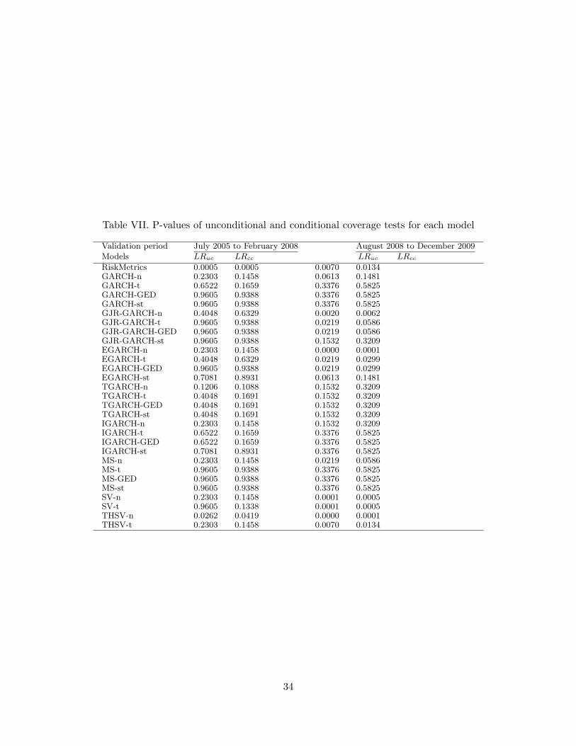
Table VII. P-values of unconditional and conditional coverage tests for each model

Validation period July 2005 to February 2008 August 2008 to December 2009Models LRuc LRcc LRuc LRcc

RiskMetrics 0.0005 0.0005 0.0070 0.0134GARCH-n 0.2303 0.1458 0.0613 0.1481GARCH-t 0.6522 0.1659 0.3376 0.5825GARCH-GED 0.9605 0.9388 0.3376 0.5825GARCH-st 0.9605 0.9388 0.3376 0.5825GJR-GARCH-n 0.4048 0.6329 0.0020 0.0062GJR-GARCH-t 0.9605 0.9388 0.0219 0.0586GJR-GARCH-GED 0.9605 0.9388 0.0219 0.0586GJR-GARCH-st 0.9605 0.9388 0.1532 0.3209EGARCH-n 0.2303 0.1458 0.0000 0.0001EGARCH-t 0.4048 0.6329 0.0219 0.0299EGARCH-GED 0.9605 0.9388 0.0219 0.0299EGARCH-st 0.7081 0.8931 0.0613 0.1481TGARCH-n 0.1206 0.1088 0.1532 0.3209TGARCH-t 0.4048 0.1691 0.1532 0.3209TGARCH-GED 0.4048 0.1691 0.1532 0.3209TGARCH-st 0.4048 0.1691 0.1532 0.3209IGARCH-n 0.2303 0.1458 0.1532 0.3209IGARCH-t 0.6522 0.1659 0.3376 0.5825IGARCH-GED 0.6522 0.1659 0.3376 0.5825IGARCH-st 0.7081 0.8931 0.3376 0.5825MS-n 0.2303 0.1458 0.0219 0.0586MS-t 0.9605 0.9388 0.3376 0.5825MS-GED 0.9605 0.9388 0.3376 0.5825MS-st 0.9605 0.9388 0.3376 0.5825SV-n 0.2303 0.1458 0.0001 0.0005SV-t 0.9605 0.1338 0.0001 0.0005THSV-n 0.0262 0.0419 0.0000 0.0001THSV-t 0.2303 0.1458 0.0070 0.0134

34