Embed Size (px)
Citation preview
Bayesian Modeling of Mortgage Prepayment Rates 1
Elmira Popova2
Operations ResearchThe University of Texas at Austin
Austin, TX 78712, [email protected]
Ivilina PopovaCeiba Asset Management, LLC
106 E 6th Street, Suite 650Austin, TX 78701, [email protected]
Edward GeorgeDepartment of Statistics
The Wharton SchoolUniversity of Pennsylvania
Philadelphia, PA 19104, [email protected]
AbstractThis paper proposes a novel approach for modeling prepayment rates of pools of mort-gages. Our goal is to establish a model that will give a good prediction for prepaymentrates for individual pools of mortgages. The model incorporates the empirical evidencethat prepayment is past dependent via Bayesian methodology. There are many factorsthat influence the prepayment behavior and for many of them there is no available (orimpossible to gather) information. We implement this issue by creating a mixture modeland construct a Markov Chain Monte Carlo algorithm to estimate the parameters. Weassess the model on a large data set from the Bloomberg Database.
Keywords: Finance, Markov Chain Monte Carlo, Bayesian statistics
1This research has been partially supported by grant #003658-0763 from the State of Texas AdvancedResearch Program
2Corresponding author
1 Introduction
Purchasing a house usually involves obtaining a loan (mortgage) originated by a financial
institution. Any standard mortgage monthly payment consists of scheduled interest and
principal. The borrower is also allowed to include additional payment toward the principle
or early payoff the whole mortgage. Refinancing of the mortgage is an example involving
such a prepayment. The issuer of the mortgage usually sells the mortgages to another
financial institution that pools them together and issues new securities, commonly known
as mortgage backed securities. The buyers of such structured products would like to know
in advance the size of the incoming prepayments (if any). To obtain the correct price one
needs to know a forecast of the prepayment.
One possible model of the prepayment is if we pretend that the borrower holds a
call option on the loan with exercise price equal to the outstanding balance ( i.e. it is a
time varying strike). Under optimal exercising conditions a mortgage can be priced as a
callable bond. One would expect that the holder will prepay when the refinancing rate
is below the mortgage rate. However, the empirical evidence, which shows very different
behavior [4], does not support such a model. As has been documented, homeowners often
prepay when it is not optimal to do so and vice versa.
The recent literature attempts to model this partially “irrational” behavior. The pre-
payment activities can be classified as either interest rate related or non-interest rate
related. The interest rate related activities (optimal prepayment) occur when the home-
owners act in order to minimize the market value of the loan. The non-interest rate
activities (suboptimal prepayments) occur for personal reasons of the borrowers, such as
divorce, job change, etc.
Two approaches have been considered for modeling prepayment. Dunn and McConnell
[4] pioneered a model based on standard contingent claim pricing theory. In their model
the prices of the mortgage backed securities (MBS) and prepayment behavior are de-
2
termined together. They assume Cox-Ingersoll-Ross interest rate model [5], introduce a
suboptimal prepayment as a Poisson event, and using non-arbitrage argument derive a
partial differential equation for the price of the security that can be solved numerically.
Suboptimal prepayment behavior was first documented in this study.
A second approach is empirical - based on historical information. Schwartz and Torous
[10] model the prepayment rate as a function of different explanatory variables, like sea-
sonality, burnout, difference between the contracting and re financing rates, and speed of
prepayment. Again using a standard arbitrage argument they derive a partial differential
equation that the MBS need to satisfy.
Richard and Roll [8] describe the prepayment model used by Goldman Sachs. They
consider four important effects: refinancing incentive, age of the mortgage, seasonality
and burnout. The conditional prepayment rate is determined as a product of functions of
the above factors. A non-linear least squares optimization procedure gives the estimated
values of the parameters. Stanton [11] presents a model that extends the option-theoretic
approach. He models the transaction costs faced by mortgage holders and assumes that
prepayment decisions occur at discrete time. This produces prepayment behavior that is
consistent with the burnout effect.
All of the existing models estimate the prepayment function by using the information
from all pools in the sample. In other words, they assume that all the pools manifest
similar prepayment behavior. Recently, Stanton [12], investigates the problem of predict-
ing the prepayment for individual pools of mortgages. He reports that in 1,000 GNMA
mortgage pools over a six and one-half year period, the unobservable heterogeneity is sta-
tistically significant. This could lead to very different prices of MBS that are backed by
different pools. One of the latest models used by Wall Street firms (BlackRock) predicts
individual pool prepayment rates based on detailed information about individual loans in
the pools.
None of the previous models has dealt with pool level predictions, and this is our main
3

research objective. Section §2 describes the nature of the raw data and how the final data
set is constructed. In sections §3 and §4 we present two prediction models: a Bayesian
mixture of regressions and a Bayesian probit mixture of regressions. In each of them we
present an extensive empirical study.
2 Data Description
We consider historical data for 78 pools of mortgages equally split between issues of
Freddie Mac and Ginnie Mae, the two major mortgage providers. To ensure the homo-
geneity of the data, we exclusively focused on 30 year fixed rate single family 8% coupon
mortgages. For these pools, Bloomberg provided general and monthly pool information
consisting of: issue date, maturity date, original amount, historical monthly prepayment
(as percentage PSA). PSA stands for the Public Securities Association convention which
assumes that 0.2% of the principle is paid in the first month, increase by 0.2% for the
following 29 months, and flattens at 6% until maturity, see [13].
The age of the mortgages varies from 5 to 25 years, and consequently, the num-
ber of data points for each pool from 60 to 300. In addition to the information pro-
vided by Bloomberg, we gathered historical long and short term interest rates from
http://www.stld.frb.org/fred/. The steps to construct the final data set are given in
the Appendix, see §6.
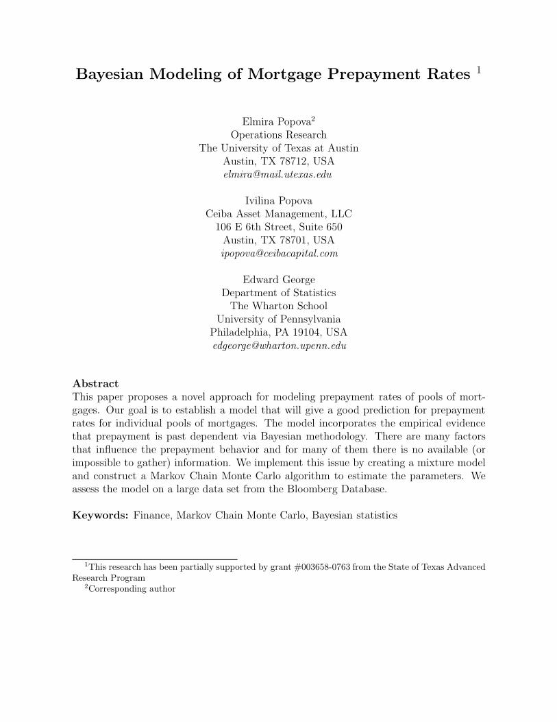
In our analysis we model the actual payment (AP) (in dollar amount) at the end of
each month t, AP (t). Preliminary analysis of the data indicates that for the most of the
pools the data exhibits a split in two groups.
Insert Figure 1 here
Figure 1 plots histograms of the logarithm of the total money paid at the end of the
month for four pools of mortgages. Note that there is a group of “small” prepayments
4
concentrated on the lower part of each graph and a group of “large” prepayments on the
upper part of each plot.
This grouping is intuitively reasonable - it seems likely that there are borrowers who
prepay small amounts each month, as well as borrowers who prepay the whole mortgage
(refinancing, selling the house, etc.) There are probably certain events that trigger the
“small” or the “large” prepayment behavior. If we knew these events and could gather
data associated with them, then we might be able to reasonably well predict the next
month prepayment. However, up to now, there is no research regarding such events, their
existence and data availability.
The Figure 1 histograms suggest that the distribution of AP is not unimodal and may
be better described with a bimodal model such as a mixture of normals. In particular,
we consider model the AP values as the realizations of n independent random variables,
x1, x2, . . . , xn from a 2-component mixture
f (xi) = pf1(xi) + (1 − p)f2(xi), i = 1, . . . , n
where fi(.) is the probability density function of a Normal distribution with parame-
ters µi and σi, i = 1, 2. We denote the unknown parameters of the mixture by θ =
(µ1, µ2, σ21, σ
22, p).
To fit and draw inference from such a model, we take a Bayesian approach which
describes the uncertainty about unknown parameters with prior probability distributions.
We proceed as in Diebolt, J. and C.P. Robert [9] and Robert, Hurn and Justel [7]. As
is well-known, Dempster, Laird and Rubin [1], any mixture model can be expressed in
terms of missing or incomplete data as follows. If, for 1 ≤ i ≤ n, zi is a 2 - dimensional
vector indicating to which component xi belongs, such that zij ∈ {0, 1}, i = 1, . . . , n,
j = 1, . . . , n, the density of the completed data (xi, zi) is
2∏j=1
pzij
j fzij
j (xi)
5
Using this representation, the parameters, θ, of the mixture model can be straightfor-
wardly estimated by a Markov Chain Monte Carlo (MCMC) algorithm, namely the Gibbs
Sampler. The general description of such an algorithm is (see [14]):
Starting with an initial value θ0
• at step m:
Generate z(m) ∼ f(z|x, θ(m)
),
Generate θ(m+1)1 ∼ π
(θ1|x, z(m), θ
(m)2 , . . . , θ(m)
s
),
...
Generate θ(m+1)s ∼ π
(θs|x, z(m), θ
(m+1)1 , . . . , θ
(m+1)s−1
)
In the above description, x is the observed data and π(θ|x, z) and f(z|x, θ) are the full
conditional distributions. The above algorithm is geometrically convergent, see Diebolt
and Robert, [9].
3 Bayesian Mixture of Regressions
The preliminary analysis of the data suggests that there are two main groups - ”small”
and ”large” prepayers. We would like to model this structure by incorporating covariates
described in the literature as important. Schwartz and Torous [10] define the following
set of variables which are significant in predicting prepayment behavior:
• X1 = the difference between the mortgage rate and the short term interest rate
• X2 = X31
• X3 captures the burnout effect - it is the logarithm of the ratio of the dollar amount
of the pool outstanding at time t, to the pool’s principle which would prevail at t
in the absence of prepayments
6

• X4 models the seasonality effect. It equals 1 for the months of May, June, July, and
August, and 0 for September, October, November, December, January, February,
March, and April.
• X5 is the spread (difference) between the long and short term interest rates.
As a forecasting model we define a Bayesian mixture of regressions similar to [7],
where Y = ln(AP (t)) is the logarithm of total money paid at the end of the month, and
X1, X2, X3, X4, X5 are the covariates defined above. The model is:
Y ∼ pN
(5∑
i=0
UiXi, W1
)+ (1 − p)N
(5∑
i=0
ViXi, W2
)
with parameters {U0, U1, U2, U3, U4, U5, V0, V1, V2, V3, V4, V5, W1, W2, p}. Note that we use
W1 and W2 to represent the precision parameters, rather than the variances, of the two
normal distributions that constitute the mixture. (Precision = 1/V ariance).
Letting M1 = (U0, U1, U2, U3, U4, U5) and M2 = (V0, V1, V2, V3, V4, V5) denoted covariate
coefficients corresponding to each of the mixture components, we consider the following
default priors for the unknown parameters. We assumed improper joint prior distribution
for (M, W ), ξ(m, w) = 1/w, w > 0 and Beta(α, β) as a prior distribution for p. Let X be
the matrix
X =
1 X11 X1
2 X13 X1
4 X15
1 X21 X2
2 X23 X2
4 X25
· · ·1 XN
1 XN2 XN
3 XN4 XN
5
Defining
m =(X
′X)−1
X′Y (1)
s2 =1
n − 2(Y − Xm)
′(Y − Xm) (2)
n1 = Number of data points in cluster 1
n2 = Number of data points in cluster 2
n1 + n2 = N
7

then under our priors, the marginal posterior distributions of the mixture parameters are
(see [9]):
Mi ∼ Multivariate t
(ni − 2, mi,
1
s2i
X′X
)(3)
Wi ∼ Gamma(
ni − 2
2,ni − 2
2s2
i
)
p ∼ Beta (n1 + α, n2 + β)
i = 1, 2
The Gibbs sampling algorithm for this setup consists of the following steps (see [9])
1. Start with initial values of the parameters θ0 = (M01 , M0
2 , W 01 , W 0
2 , p0)
2. Allocate each Yi to the first or second mixture based on odds ratio
P [zi = 0|θ, y]
P [zi = 1|θ, y]
This part of the algorithm will generate Zi = 0 if the odds ratio is less than 1 and
Zi = 1 if it is greater than 1.
3. Now each the points has been assigned either to cluster 1 or cluster 2. Given that
we are in cluster i, i = 1, 2, we simulate θ from the marginal distributions (3)
4. Repeat the above steps M times (number of simulation runs)
We used the uniform random number generator written by P. L’Ecuyer (see [6]) and non
uniform random number algorithms from Devroye, [3].
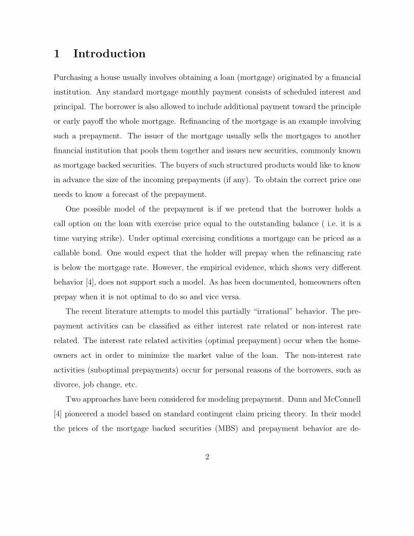
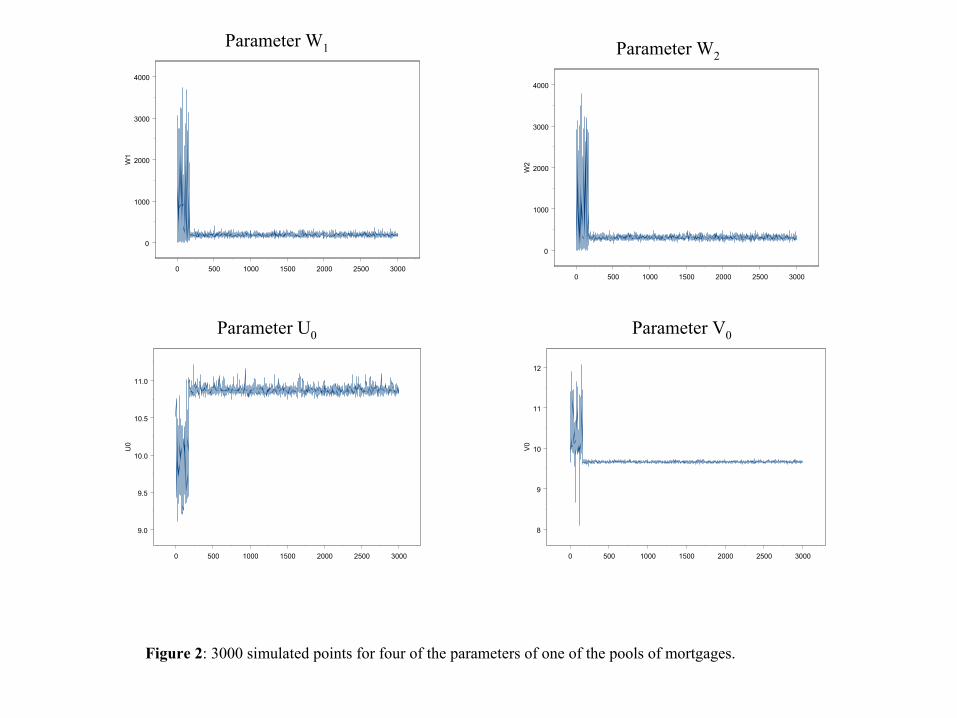
The length of our simulation runs is 5000, the algorithm is implemented in C++ and
run on 2.37GHz Pentium. As with any MCMC algorithm, there is a transient period at
the beginning of the simulation. Figure 2 shows the actual simulated points for one of
the parameters of one of the pools of mortgages. Based on the observed patterns for the
moving average process of the simulated values we dropped the first 1000 simulated values
8
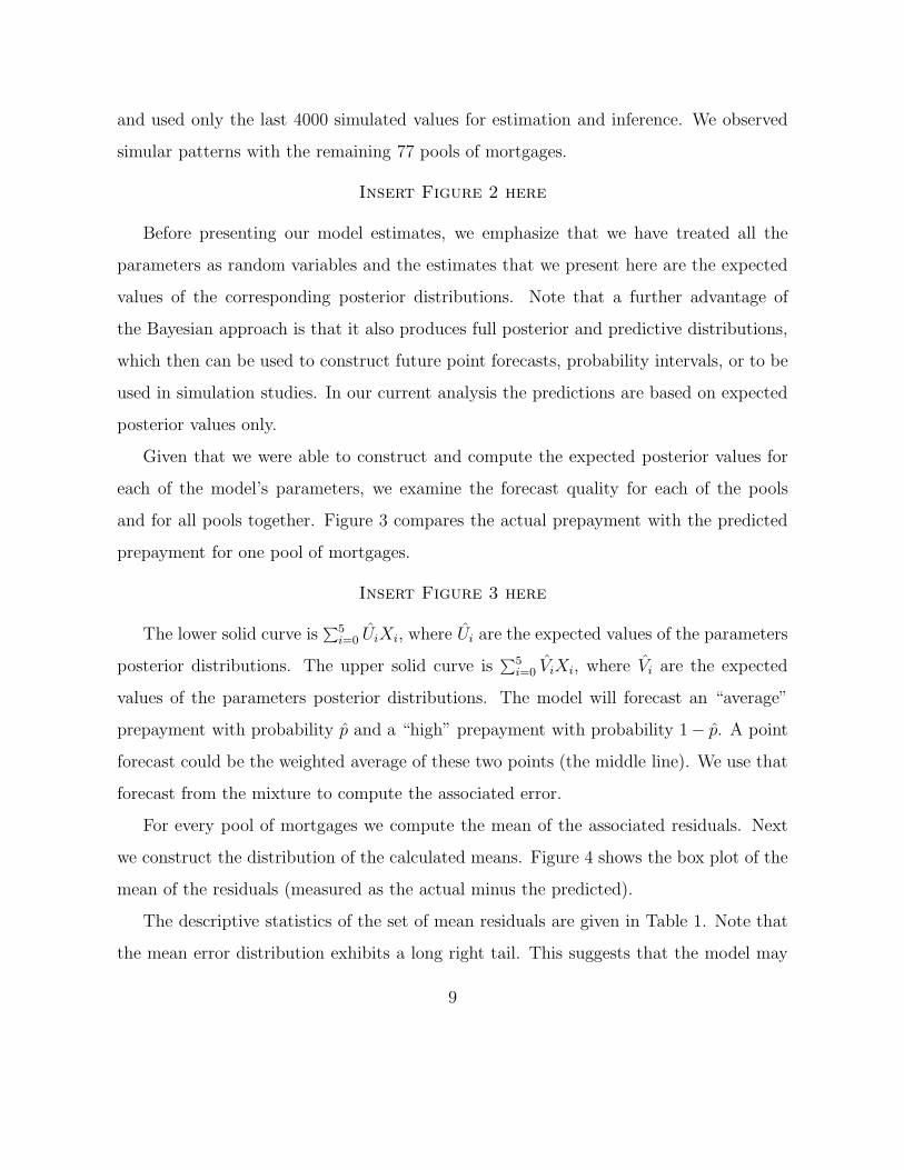
and used only the last 4000 simulated values for estimation and inference. We observed
simular patterns with the remaining 77 pools of mortgages.
Insert Figure 2 here
Before presenting our model estimates, we emphasize that we have treated all the
parameters as random variables and the estimates that we present here are the expected
values of the corresponding posterior distributions. Note that a further advantage of
the Bayesian approach is that it also produces full posterior and predictive distributions,
which then can be used to construct future point forecasts, probability intervals, or to be
used in simulation studies. In our current analysis the predictions are based on expected
posterior values only.
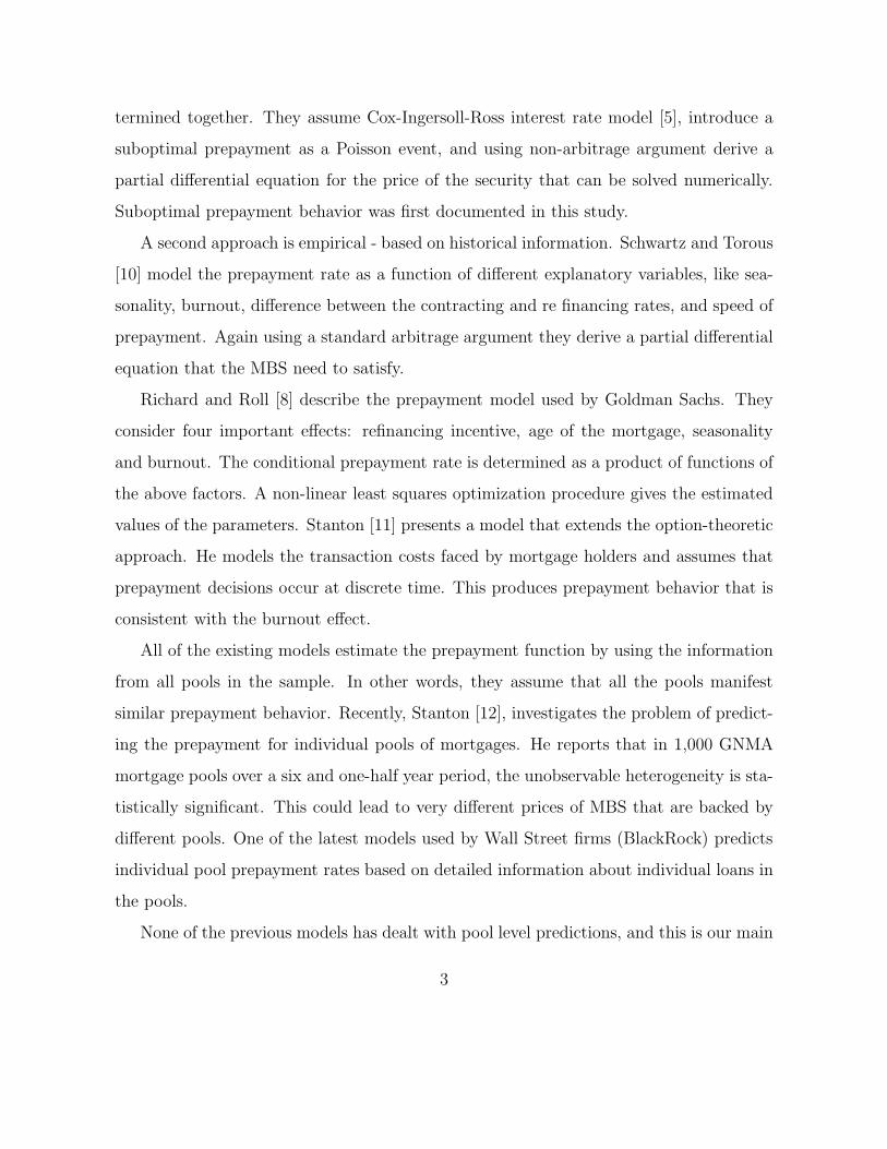
Given that we were able to construct and compute the expected posterior values for
each of the model’s parameters, we examine the forecast quality for each of the pools
and for all pools together. Figure 3 compares the actual prepayment with the predicted
prepayment for one pool of mortgages.
Insert Figure 3 here
The lower solid curve is∑5
i=0 UiXi, where Ui are the expected values of the parameters
posterior distributions. The upper solid curve is∑5
i=0 ViXi, where Vi are the expected
values of the parameters posterior distributions. The model will forecast an “average”
prepayment with probability p and a “high” prepayment with probability 1− p. A point
forecast could be the weighted average of these two points (the middle line). We use that
forecast from the mixture to compute the associated error.
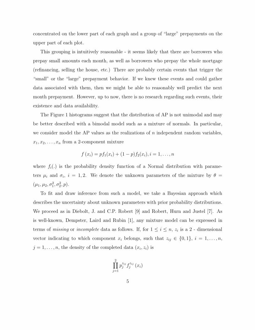
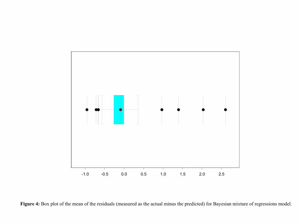
For every pool of mortgages we compute the mean of the associated residuals. Next
we construct the distribution of the calculated means. Figure 4 shows the box plot of the
mean of the residuals (measured as the actual minus the predicted).
The descriptive statistics of the set of mean residuals are given in Table 1. Note that
the mean error distribution exhibits a long right tail. This suggests that the model may
9
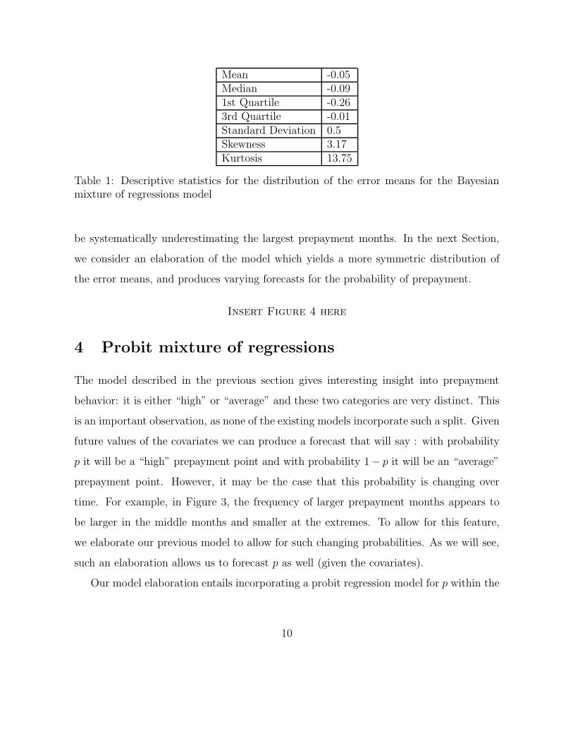
Mean -0.05Median -0.091st Quartile -0.263rd Quartile -0.01Standard Deviation 0.5Skewness 3.17Kurtosis 13.75
Table 1: Descriptive statistics for the distribution of the error means for the Bayesianmixture of regressions model
be systematically underestimating the largest prepayment months. In the next Section,
we consider an elaboration of the model which yields a more symmetric distribution of
the error means, and produces varying forecasts for the probability of prepayment.
Insert Figure 4 here
4 Probit mixture of regressions
The model described in the previous section gives interesting insight into prepayment
behavior: it is either “high” or “average” and these two categories are very distinct. This
is an important observation, as none of the existing models incorporate such a split. Given
future values of the covariates we can produce a forecast that will say : with probability
p it will be a “high” prepayment point and with probability 1− p it will be an “average”
prepayment point. However, it may be the case that this probability is changing over
time. For example, in Figure 3, the frequency of larger prepayment months appears to
be larger in the middle months and smaller at the extremes. To allow for this feature,
we elaborate our previous model to allow for such changing probabilities. As we will see,
such an elaboration allows us to forecast p as well (given the covariates).
Our model elaboration entails incorporating a probit regression model for p within the
10
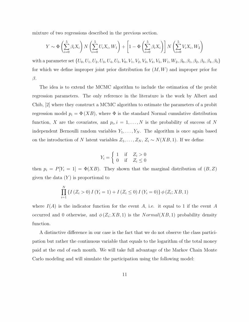
mixture of two regressions described in the previous section.
Y ∼ Φ
(5∑
i=0
βiXi
)N
(5∑
i=0
UiXi, W1
)+
[1 − Φ
(5∑
i=0
βiXi
)]N
(5∑
i=0
ViXi, W2
)
with a parameter set {U0, U1, U2, U3, U4, U5, V0, V1, V2, V3, V4, V5, W1, W2, β0, β1, β2, β3, β4, β5}for which we define improper joint prior distribution for (M, W ) and improper prior for
β.
The idea is to extend the MCMC algorithm to include the estimation of the probit
regression parameters. The only reference in the literature is the work by Albert and
Chib, [2] where they construct a MCMC algorithm to estimate the parameters of a probit
regression model pi = Φ (XB), where Φ is the standard Normal cumulative distribution
function, X are the covariates, and pi, i = 1, . . . , N is the probability of success of N
independent Bernoulli random variables Y1, . . . , YN . The algorithm is once again based
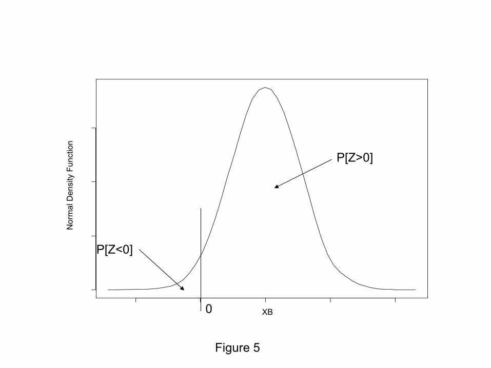
on the introduction of N latent variables Z1, . . . , ZN , Zi ∼ N(XB, 1). If we define
Yi =
{1 if Zi > 00 if Zi ≤ 0
then pi = P [Yi = 1] = Φ(XB). They shown that the marginal distribution of (B, Z)
given the data (Y ) is proportional to
N∏i=1
{I (Zi > 0) I (Yi = 1) + I (Zi ≤ 0) I (Yi = 0)}φ (Zi; XB, 1)
where I(A) is the indicator function for the event A, i.e. it equal to 1 if the event A
occurred and 0 otherwise, and φ (Zi; XB, 1) is the Normal(XB, 1) probability density
function.
A distinctive difference in our case is the fact that we do not observe the class partici-
pation but rather the continuous variable that equals to the logarithm of the total money
paid at the end of each month. We will take full advantage of the Markov Chain Monte
Carlo modeling and will simulate the participation using the following model:
11

Define
Y ∼ Normal(µδ, σ
2δ
)(4)
δ = 1 (Z > 0) =
{1 if Z > 00 if Z ≤ 0
(5)
Z ∼ Normal(BX, 1) (6)
µ0 =5∑
i=0
UiXi (7)
µ1 =5∑
i=0
ViXi (8)
σ2i = 1/Wi, i = 1, 2 (9)
Then given δi, Y, i = 1, . . . , n we simulate U0, U1, U2, U3, U4, U5, V0, V1, V2, V3, V4, V5, W1, W2;
given U0, U1, U2, U3, U4, U5, V0, V1, V2, V3, V4, V5, W1, W2, Y we simulate δ1, . . . , δn.
If we denote by Θ = (µ0, µ1, σ20, σ
21) the marginal distribution of (Z, B) given (Y, Θ) is
π (Z, B|Y, Θ) ∝ Cπ(B)N∏
i=1
{1 (Zi > 0) φ(µ1,σ2
1)(yi) + 1 (Zi ≤ 0) φ(µ0,σ2
0)(yi)
}φ(XB,1) (Zi)
where φ(µ,σ2)(•) is the Normal(µ, σ2) probability density function.
We need to be able to simulate from that distribution. In Albert and Chib case it is
the truncated Normal either at the left or right by 0 depending on the observed value of
the binary data (see Figure 5).
Insert Figure 5 here
In our case the distribution to the left of 0 does not have to be the same Normal
distribution. We propose the following sampling algorithm:
Define
12

a0 = φ(µ0,σ20)
(yi) (10)
a1 = φ(µ1,σ21)
(yi) (11)
α =a0Φ(XB,1)(0)
a0Φ(XB,1)(0) + a1
[1 − Φ(XB,1)(0)
] (12)
β =a1
[1 − Φ(XB,1)(0)
]a0Φ(XB,1)(0) + a1
[1 − Φ(XB,1)(0)
] (13)
Then given the observed data yi the sampling algorithm for Z is:
• Step 1: With probability α simulate Z from N(XB, 1) truncated at left by 0.
• Step 2: With probability β = 1 − α simulate Z from N(XB, 1) truncated at right
by 0.
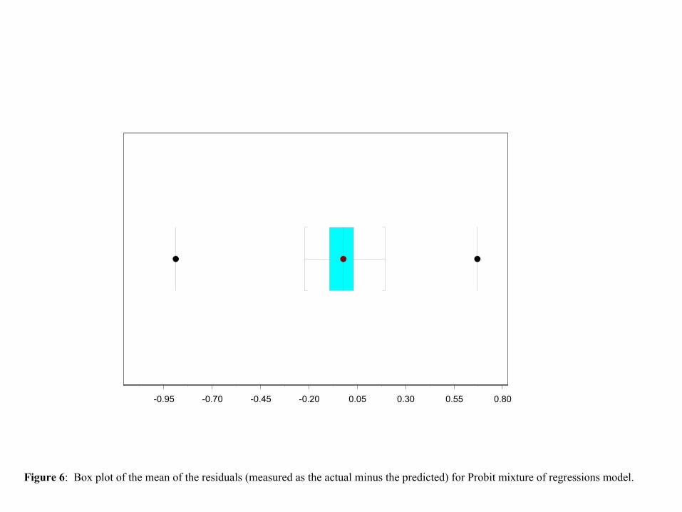
To gauge the quality of fit of this elaborated model, we computed the residual differ-
ences between the observed AP values and the corresponding posterior mean. Descriptive
statistics of these residuals are reported in Table 2, and a box plot of these residuals is
provided in Figure 6.
Insert Figure 6 here
Comparison with Table 1 shows that the standard deviation has dropped very sub-
stantially from 0.5 to 0.12, a reduction of more than 75%. Thus, the overall fit of the
enhanced model is much better. Comparison of Figure 4 with Figure 6 reveals that the
residuals have become much more symmetric. This is also evidence by the drastic change
in the coefficient of skewness from 3.17 to −1.19. By allowing the p to vary, the elaborated
model has shifted the overall posterior mean upwards the larger prepayment months.
13
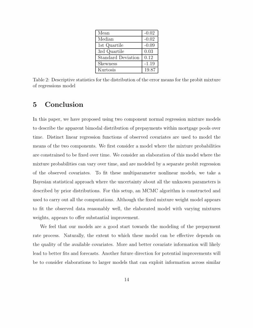
Mean -0.02Median -0.021st Quartile -0.093rd Quartile 0.03Standard Deviation 0.12Skewness -1.19Kurtosis 19.87
Table 2: Descriptive statistics for the distribution of the error means for the probit mixtureof regressions model
5 Conclusion
In this paper, we have proposed using two component normal regression mixture models
to describe the apparent bimodal distribution of prepayments within mortgage pools over
time. Distinct linear regression functions of observed covariates are used to model the
means of the two components. We first consider a model where the mixture probabilities
are constrained to be fixed over time. We consider an elaboration of this model where the
mixture probabilities can vary over time, and are modeled by a separate probit regression
of the observed covariates. To fit these multiparameter nonlinear models, we take a
Bayesian statistical approach where the uncertainty about all the unknown parameters is
described by prior distributions. For this setup, an MCMC algorithm is constructed and
used to carry out all the computations. Although the fixed mixture weight model appears
to fit the observed data reasonably well, the elaborated model with varying mixtures
weights, appears to offer substantial improvement.
We feel that our models are a good start towards the modeling of the prepayment
rate process. Naturally, the extent to which these model can be effective depends on
the quality of the available covariates. More and better covariate information will likely
lead to better fits and forecasts. Another future direction for potential improvements will
be to consider elaborations to larger models that can exploit information across similar
14

mortgage pools. One such elaboration would be a hierarchical Bayes model that treats the
parameters of each pool as a sample from a superpopulation model. Such an elaboration
would be particularly natural given the Bayesian treatment we have here considered.
6 Appendix
The construction of the data set consists of several steps.
1. Compute the conditional prepayment rate using the formula
CPR = PSA(standard).PSA(historical)/100,
where PSA(historical) comes from the data set.
2. Compute the single monthly mortality rate, SMM = 1 − (1 − CPR)112 .
3. For t = 0, . . . , 360 compute the monthly payment as MP =FaceV alue[ 0.085
12 ][1+ 0.08512 ]
t
[1+ 0.08512 ]
t−1
and the interest payment as IP = FaceV alue[
0.08512
].
4. Compute the scheduled principle, SP = MP − IP .
5. Compute the nonscheduled prepayment, NPP = SMM(FaceV alue−SP ), and the
actual payment, AP = SP + NNP
References
[1] N. M. Laird A. P. Dempster and D. B. Rubin. Maximum likelihood from incomplete
data via the em algorithm (with discussion). Journal of the Royal Statistical Society,
B 39:1–38, 1977.
[2] J. H. Albert and S. Chib. Bayesian analysis of binary and polychotomous response
data. Journal of the american statistical association, 88(422):669–679, 1993.
15

[3] L. Devroye. Non uniform random variate generation. Springer Verlag, 1986.
[4] K. Dunn and J. McConnell. Valuation of gnma mortgage-backed securities. The
Journal of Finance, XXXVI(3):599–616, 1981.
[5] J. E. Ingersoll J. C. Cox and S. A. Ross. A theory of the term structure of interest
rates. Econometrica, 53(2):385 – 407, 1985.
[6] P. Lecuyer. http://www.iro.umontreal.ca/ lecuyer.
[7] C. P. Robert M. Hurn, A. Justel. Estimating mixtures of regressions. Journal of
Compuational and Graphical Statistics, 12(1):1–25, 2003.
[8] R. Richard and R. Roll. Modeling prepayments on fixed-rate mortgage-backed secu-
rities. Journal of Portfolio Management, 15(3):73–82, 1989.
[9] J. Diebolt C. P. Robert. Estimation of finite mixture distributions through bayesian
sampling. Journal of the Royal Statistical Society, B 56(2):363–375, 1994.
[10] E. Schwartz and W. Torous. Prepayment and the valuation of mortgage-backed
securities. Journal of Finance, 44(2):375–392, 1989.
[11] R. Stanton. Rational prepayment and the valuation of mortgage-backed securities.
Review of Financial Studies, 8(3):677–708, 1996.
[12] R. Stanton. Unobservable heterogeneity and rational learning: Pool-specific versus
generic mortgage-backed security prices. Journal of Real Estate and Economics,
12:243–263, 1996.
[13] Suresh M. Sundaresan. Fixed income markets and their derivatives. South-Western
College Publishing, 1997.
16

[14] S. Richardson W. R. Gilks and D. J. Spiegelhalter. Markov chain Monte Carlo in
practice. Chapman and Hall, 1996.
17
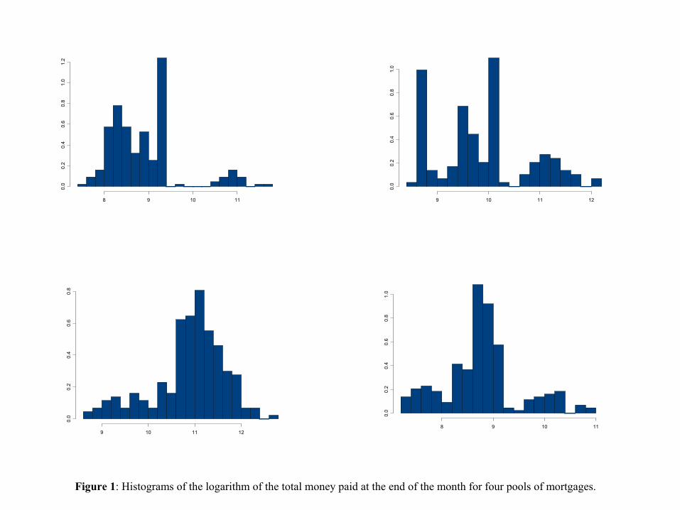
Figure 1: Histograms of the logarithm of the total money paid at the end of the month for four pools of mortgages.
8 9 10 11
0.0
0.2
0.4
0.6
0.8
1.0
1.2
8 9 10 11
0.0
0.2
0.4
0.6
0.8
1.0
9 10 11 12
0.0
0.2
0.4
0.6
0.8
9 10 11 12
0.0
0.2
0.4
0.6
0.8
1.0
0 500 1000 1500 2000 2500 3000
0
1000
2000
3000
4000
W1
0 500 1000 1500 2000 2500 3000
0
1000
2000
3000
4000
W2
0 500 1000 1500 2000 2500 3000
9.0
9.5
10.0
10.5
11.0
U0
0 500 1000 1500 2000 2500 3000
8
9
10
11
12
V0
Figure 2: 3000 simulated points for four of the parameters of one of the pools of mortgages.
Parameter W1 Parameter W2
Parameter U0 Parameter V0
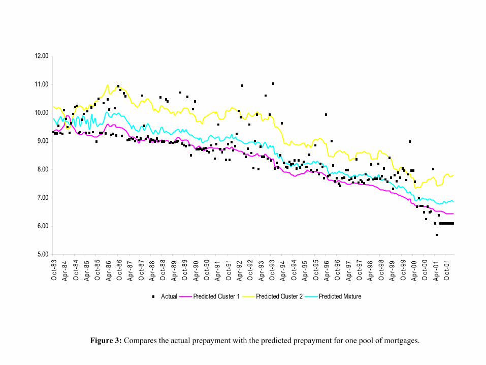
Figure 3: Compares the actual prepayment with the predicted prepayment for one pool of mortgages.
5.00
6.00
7.00
8.00
9.00
10.00
11.00
12.00O
ct-8
3Ap
r-84
Oct
-84
Apr-
85O
ct-8
5Ap
r-86
Oct
-86
Apr-
87O
ct-8
7Ap
r-88
Oct
-88
Apr-
89O
ct-8
9Ap
r-90
Oct
-90
Apr-
91O
ct-9
1Ap
r-92
Oct
-92
Apr-
93O
ct-9
3Ap
r-94
Oct
-94
Apr-
95O
ct-9
5Ap
r-96
Oct
-96
Apr-
97O
ct-9
7Ap
r-98
Oct
-98
Apr-
99O
ct-9
9Ap
r-00
Oct
-00
Apr-
01O
ct-0
1
Actual Predicted Cluster 1 Predicted Cluster 2 Predicted Mixture
-1.0 -0.5 0.0 0.5 1.0 1.5 2.0 2.5
Figure 4: Box plot of the mean of the residuals (measured as the actual minus the predicted) for Bayesian mixture of regressions model.
XB
Nor
mal
Den
sity
Fun
ctio
n
0
P[Z>0]
P[Z<0]
Figure 5
-0.95 -0.70 -0.45 -0.20 0.05 0.30 0.55 0.80
Figure 6: Box plot of the mean of the residuals (measured as the actual minus the predicted) for Probit mixture of regressions model.