Embed Size (px)
Citation preview
1
(PAPER FOR PRESENTATION AT THE 2004 AFIR COLLOQIUM BOSTON, MA, NOVEMBER 7-10, 2004)
ON MORTGAGE PREPAYMENT AND DEFAULT:
A HISTORICAL DISTRIBUTION ANALYSIS APPROACH
Marco van Akkeren1
Henry W. Hansen2
PMI Mortgage Insurance Co., Walnut Creek, CA, USA
July 2004
Abstract – We present evidence on mortgage default and prepayment distributions based on
a subset of PMI Mortgage Insurance Co. data. We show that marginal claim distributions for
specific asset classes are varied and skewed in nature, and may be joined through an
estimated covariance matrix and Monte-Carlo simulation. Ignoring correlation effects
underestimates tail portfolio claim probabilities, which is illustrated through a set of
examples. A ranking of asset classes defined by product type, Loan-to-Value-ratio (LTV),
credit quality, and seasoning is presented based on unexpected claims and select measures of
persistency. The impact of geographical diversification is examined to show that increasing
diversification raises the expected claim rate, but lowers the unexpected claim rate.
Keywords: mortgage, prepayment, default, distribution analysis, Monte-Carlo simulation, portfolio management, credit risk, market risk, asset classes, covariance estimation, methods of moments, maximum likelihood
MSC2000 Classification: 62F07, 62F10, and 62P05
Full Affiliation1: Director, Mortgage Analytics, PMI Mortgage Insurance Co. Full Affiliation2: VP, Actuarial, Pricing & Mortgage Analytics, PMI Mortgage Insurance Co. Address: 3003 Oak Road, Walnut Creek, CA 94597 Tel1: (925) 658-6166 Tel2: (925) 658-6333 Fax: (925) 658-6780 E-mail: [email protected], [email protected]
2
I. Introduction
The analysis of claim and prepayment distributions in the U.S. mortgage insurance
industry has in recent years seen a rebound in interest by risk management practitioners
driven by a search for improved capital management tools. This trend followed earlier
improvement in capital management methods in the U.S. property & casualty (P&C)
insurance industry (Nakada, Shah, Koyluoglu, and Collignon, 1999), which came on the
heels of major capital allocation changes in the U.S. Banking and Investment community that
began in the late 1980s. At the core of these changes are questions regarding capitalization
and whether capital reserves are sufficient or inadequate to cover losses in a severe economic
downturn.
Within the U.S. mortgage insurance industry there exist several standards for
measuring capital adequacy: statutory, regulatory, rating agency, and internal corporate
capital requirements. One internal approach that has gained popularity in recent years is that
of Economic Capital and Risk Adjusted Return on Capital (RAROC) (Zaik, Walter, and
Kelling, 1996). Economic capital is the amount of capital needed over a specific time horizon
to support enterprise wide risk to a given level of solvency. More precisely, it can be defined
as the difference between expected value and the pth quantile of a company’s value
distribution that incorporates all the company’s risk in terms of assets and liabilities. In
banking or a trading environment, this time period tends to be relatively short lived: several
weeks, months or 1 year at most. For mortgage insurance companies, however, capital is set
aside to cover a severe economic downturn over the life of a loan. Therefore, Value-At-Risk
(VAR) analysis (Holton, 2003) differs from the Economic Capital framework in that VAR
typically takes an approach that estimates the distribution of short-term trading losses using
market value accounting and exposure to market risk. Economic capital takes a more long-
term view and uses distributional analysis based on historical data instead of the short-term
simulation driven techniques.
Traditionally, a grouping of risk is applied to facilitate risk management (Crouhy,
Galai, and Mark, 2001). We have identified four risk groupings that mortgage insurers face
and that are also used at most banks, namely: (i) credit risk, (ii) market risk, (iii) business
risk, and (iv) operational risk. In the property and casualty (P&C) insurance industry, risk
management practitioners are faced with an additional layer of risk, which is catastrophe risk.
Variability in losses and company value in this case would result from natural disasters such
as earthquakes, hurricanes, or tornadoes, but since mortgage insurance coverage does not

3
extend to losses resulting from property damage, this dimension may be ignored. Credit risk
(Duffie and Singleton, 2003) in consumer lending is primarily quantified through measures of
payment behavior and not personal income. The Fair Isaac & Co. credit scores, or FICO
scores, are recorded and maintained by three principal credit agencies of Experian, Trans-
Union, and Equifax and they represent the standard for measuring consumer credit risk today.
The second risk grouping listed above, namely market risk, could entail one or more of the
following: interest rates, foreign-exchange (FX) rates, commodity prices, equity prices, and
credit spread. In the mortgage insurance industry, interest rates and home price appreciation
are the main driving variables for market risk (Hayre, 2001). Interest rates are important,
because they tend to drive prepayment behavior especially in a decreasing rate environment,
while house price appreciation is an important consideration for the borrower to default on
his mortgage. The borrower has an incentive to default if the market price of his home is
below the purchase price, and Loan-to-Value (LTV) ratio is a measure that can also be
estimated after origination. Business risk is identified as changes in market share and
volumes that result from a competitive market environment and historical sales and market
share data can be used to quantify this uncertainty. Finally, operational risk is the risk of loss
resulting from inadequate or failed business practices, processes or employees and has
become a popular topic for research and analysis in recent years. Operational risk generally is
difficult to quantify, as there tends to be limited internal data available to estimate loss
distributions. There are methods to supplement internal observations with external data, but
care must be taken to ensure compatibility through proper scaling and data adjustments.
Examples of operational risk include, but are not limited to internal/external theft and fraud,
unauthorized transactions, business interruptions and systems failure.
In terms of a historical perspective, there have been a number of risk events that have
shocked financial markets both domestically and internationally. Among the most recent and
prominent of these are the following: the 1994 bond sell-off and interest rate increase, the
1992 Hurricane Andrew and its impact on the P&C insurance/reinsurance industry, the 1997
emerging markets crisis followed by the 1998 Russia crisis and the collapse of Long Term
Capital Management (LTCM), the 2000 U.S. recession and start of high volatility period in
equity markets, September 11, 2001 followed by major corporate credit default and
bankruptcies. The mortgage industry while certainly affected by interest-rate shocks has also
been hurt by sustained local economic downturns and the impact that has had on mortgage
default. Since economic capital is set aside to survive the rare or “tail” event that occurs with
a certain probability, it becomes very important to estimate the company’s underlying value
4
distribution accurately so that the company is sufficiently capitalized to sustain a business
cycle downturn with a likelihood of occurrence that is quantified by the tail probability.
As an integral component in estimating the company’s value distribution, this study is
focused on estimating default frequency and persistency (prepayment) distributions for a set
of asset classes that we shall define below. Our findings suggest that certain asset classes
have higher expected default rates than others, but that the unexpected claims for these
classes do not necessarily follow the same trend. Moreover, some asset classes are more
strongly correlated than others, and that ignoring these correlating effects will underestimate
portfolio default frequency distributions. A comparative analysis is presented to show which
asset classes have higher unexpected claim rates than others, but also in terms of prepayment
speeds. The latter is important, because it gives us an indication of average duration and the
amount of mortgage insurance premium that can be expected on average, but also in stress
cases. Default frequency distributions are presented to show the impact of geographical
diversification on the claim frequency distribution and show that increasing diversification
raises the expected claim rate but lowers the unexpected claims as the distribution tails
shrink.
This paper is organized as follows: following the introduction, Section 2 investigates
the impact of geographical diversification on the claim frequency distribution. Section 3
reveals our approach to portfolio segmentation and defines specific asset classes based on
idiosyncratic properties of these classes. Section 4 presents a Monte-Carlo simulation
algorithm through which the effects of asset correlation can be incorporated in deriving
frequency distributions for a portfolio of loans. The following section discusses the properties
of these asset classes based on persistency distributions. In conclusion, we summarize our
major research findings and suggest future paths of research and interest.
II. The Impact of Geographic Diversification
The U.S. Mortgage industry market risk primarily revolves around interest rate and
house price shock. The impact of falling interest rates acts to increase the incentive for
borrowers to refinance their mortgage at a lower note rate. Therefore, interest rate shocks
generally will primarily impact revenue and losses only secondarily. There is however an
underlying association between interest rates and macroeconomic conditions. Lower interest
rates tend to be associated with a poor U.S. economy, which in turn could impact the demand
5
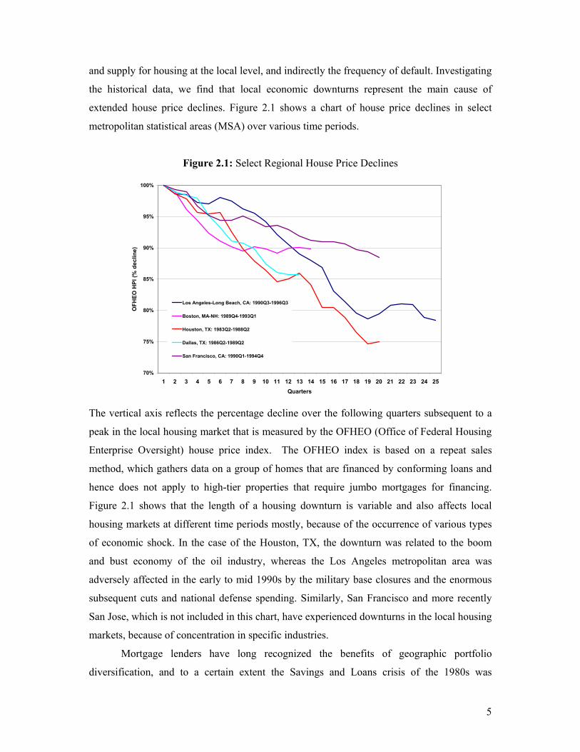
and supply for housing at the local level, and indirectly the frequency of default. Investigating
the historical data, we find that local economic downturns represent the main cause of
extended house price declines. Figure 2.1 shows a chart of house price declines in select
metropolitan statistical areas (MSA) over various time periods.
Figure 2.1: Select Regional House Price Declines
70%
75%
80%
85%
90%
95%
100%
1 2 3 4 5 6 7 8 9 10 11 12 13 14 15 16 17 18 19 20 21 22 23 24 25Quarters
OFH
EO H
PI (%
dec
line)
Los Angeles-Long Beach, CA: 1990Q3-1996Q3
Boston, MA-NH: 1989Q4-1993Q1
Houston, TX: 1983Q2-1988Q2
Dallas, TX: 1986Q2-1989Q2
San Francisco, CA: 1990Q1-1994Q4
The vertical axis reflects the percentage decline over the following quarters subsequent to a
peak in the local housing market that is measured by the OFHEO (Office of Federal Housing
Enterprise Oversight) house price index. The OFHEO index is based on a repeat sales
method, which gathers data on a group of homes that are financed by conforming loans and
hence does not apply to high-tier properties that require jumbo mortgages for financing.
Figure 2.1 shows that the length of a housing downturn is variable and also affects local
housing markets at different time periods mostly, because of the occurrence of various types
of economic shock. In the case of the Houston, TX, the downturn was related to the boom
and bust economy of the oil industry, whereas the Los Angeles metropolitan area was
adversely affected in the early to mid 1990s by the military base closures and the enormous
subsequent cuts and national defense spending. Similarly, San Francisco and more recently
San Jose, which is not included in this chart, have experienced downturns in the local housing
markets, because of concentration in specific industries.
Mortgage lenders have long recognized the benefits of geographic portfolio
diversification, and to a certain extent the Savings and Loans crisis of the 1980s was
6
exacerbated from a lack of diversification. Increasing the degree of geographical
diversification of a mortgage portfolio raises the expected claim frequency rate, however
when we turn to the historical data, how is the risk level affected in term of unexpected
claims given the experience of select housing market downturns? Our approach to answering
this question is to analyze PMI Group quarterly historical observations on claim frequency
default from 1977-2003 by aggregating PMI’s experience into 4 distinct geographical
categories: (a) U.S., (b) the nine census regions, (c) state, and (d) MSA. We then use
Maximum-Likelihood (ML) estimation and Method-of-Moments (MOM) (Rice, 1995) to
estimate a variety of distributions, which may be characterized by a single parameter such as
Poisson or Exponential, two parameter distributions such as Beta, or three parameter
distributions of which the Generalized Gamma is an example. Specifically, since claim rate
xi≥0 is weakly bounded by zero, we ignore short-term correlation effects between book
quarter claim rates, or Cov(xi, xj)=0 for i≠j, and estimate the parameters of the Generalized
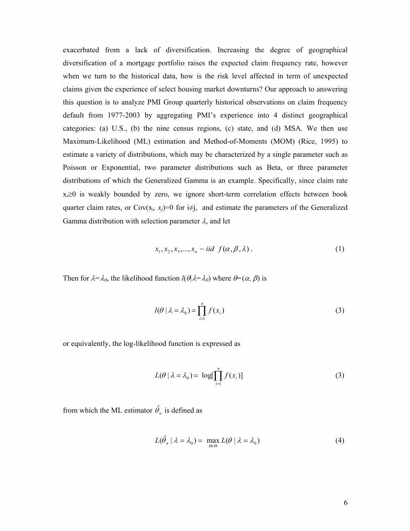
Gamma distribution with selection parameter λ, and let
),,(~,...,,, 321 λβαfiidxxxx n . (1)
Then for λ=λ0, the likelihood function l(θ|λ=λ0) where θ=(α, β) is
)()|(1
0 ∏=
==n
iixfl λλθ (3)
or equivalently, the log-likelihood function is expressed as
)]([log)|(1
0 ∏=
==n
iixfL λλθ (3)
from which the ML estimator nθ is defined as
)|(max)|ˆ( 00 λλθλλθθ
===Θ∈
LL n (4)

7
The statistical properties of the Maximum-Likelihood estimator are known to be
asymptotically normal, efficient, and unbiased. In smaller samples, estimates may not be as
efficient as other estimation techniques. Moreover, one consequence of using the maximum
likelihood procedure is that the moments of the estimated distribution do not necessarily
equal the empirical moments based on the sample observations. If such a condition is
preferred, the Method-of-Moments (MOM) approach may be applied instead where the
optimal estimate is defined as,
]0);(1[argˆ1
== ∑=Θ∈
n
iixh
nθθ
θ (5)
and is the argument that solves the empirical representation of a k-dimensional vector
function of moment conditions, E[h(x;θ)]=0. Estimation results are presented in Table 1
below, with standard errors of the estimates provided in parentheses.
Table 1
Estimated Distribution Parameters
Diversification Distribution α β
U.S. Lognormal -2.948 (0.076) 0.614 (0.069)
Census Region Gamma 0.752 (0.063) 0.074 (0.007)
State Beta 0.393 (0.017) 7.720 (0.391)
MSA Beta 0.337 (0.008) 6.689 (0.191)
In the case of the Lognormal distribution, α is as in E(xi)=α and [Var(xi)]1/2= β is the standard
deviation distribution, while for the Gamma, β is defined as in E(xi)= α * β. In testing for the
best fit to the hypothesized distribution, we have used three different statistical tests, namely
the Kolmogorov-Smirnov, Andersen-Darling, and Cramer-von Mises. This is because each
test emphasizes a different criterion. The K-S statistic emphasizes the difference between the
tails of the distribution, whereas the other two methods apply a means of weighting all
quantile differences and not just the maximum difference between the distributions. Table 1
shows that a specific probability distribution yields the best goodness of fit, depending on the
degree of geographic diversification.
8
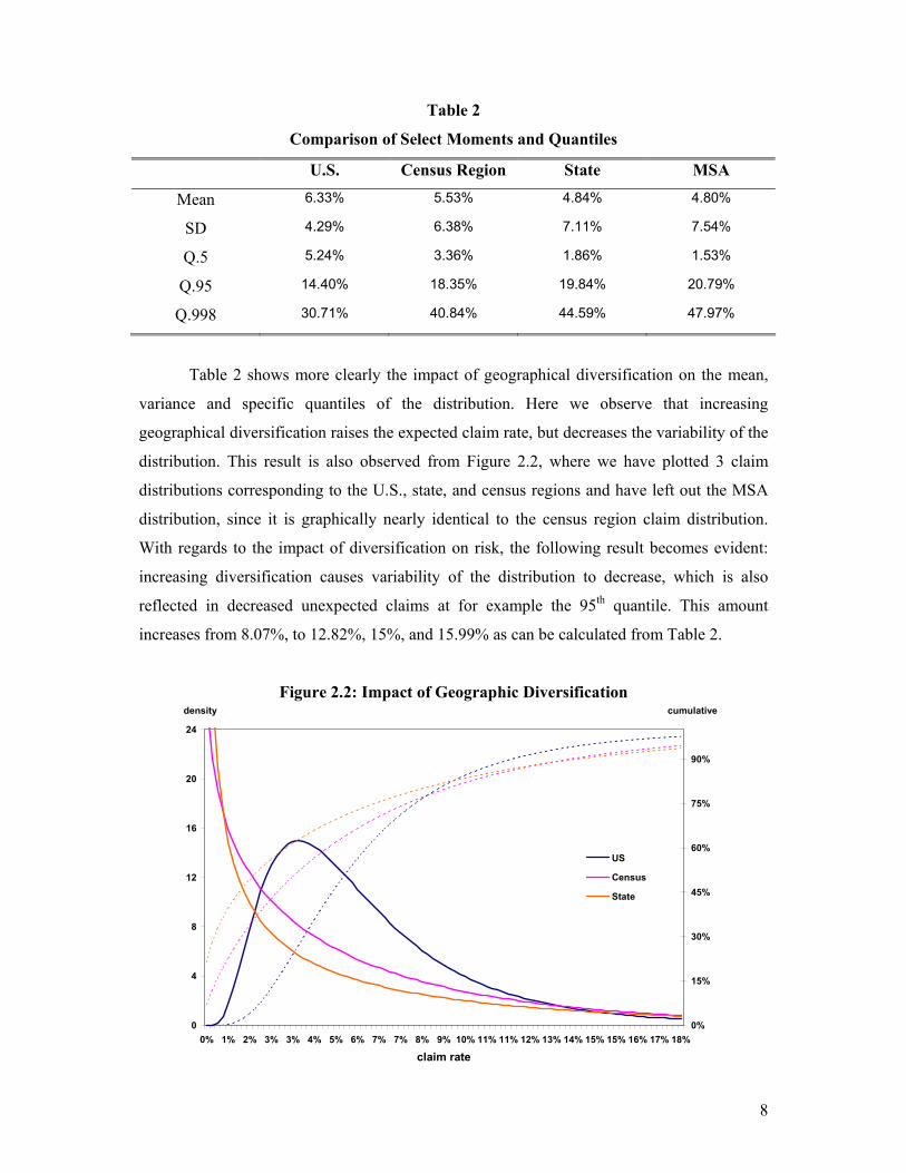
Table 2
Comparison of Select Moments and Quantiles
U.S. Census Region State MSA
Mean 6.33% 5.53% 4.84% 4.80%
SD 4.29% 6.38% 7.11% 7.54%
Q.5 5.24% 3.36% 1.86% 1.53%
Q.95 14.40% 18.35% 19.84% 20.79%
Q.998 30.71% 40.84% 44.59% 47.97%
Table 2 shows more clearly the impact of geographical diversification on the mean,
variance and specific quantiles of the distribution. Here we observe that increasing
geographical diversification raises the expected claim rate, but decreases the variability of the
distribution. This result is also observed from Figure 2.2, where we have plotted 3 claim
distributions corresponding to the U.S., state, and census regions and have left out the MSA
distribution, since it is graphically nearly identical to the census region claim distribution.
With regards to the impact of diversification on risk, the following result becomes evident:
increasing diversification causes variability of the distribution to decrease, which is also
reflected in decreased unexpected claims at for example the 95th quantile. This amount
increases from 8.07%, to 12.82%, 15%, and 15.99% as can be calculated from Table 2.
Figure 2.2: Impact of Geographic Diversification
0
4
8
12
16
20
24
0% 1% 2% 3% 3% 4% 5% 6% 7% 7% 8% 9% 10% 11% 11% 12% 13% 14% 15% 15% 16% 17% 18%
claim rate
density
0%
15%
30%
45%
60%
75%
90%
cumulative
US
Census
State
9
III. Portfolio Segmentation
In order to facilitate risk management, segmentation of a portfolio into distinct asset classes is
traditionally applied with the purpose finding an optimal combination of these classes given a
risk-return preference set or any other specific objective function. Risk is generally identified
by a dispersion measure of the distribution. However, as our results will indicate when
dealing with highly skewed distributions, robust statistics such as quantiles may be more
preferable, because it provides a more direct probabilistic interpretation of unexpected
claims. The goal is then to define a set of classes that are manageable in size yet have the
same idiosyncratic properties. In the case of U.S. residential mortgages, our approach is to
identify a set of classes that incorporates: (a) mortgage product type, (b) credit quality
segmentation, (c) LTV, and (d) seasoning.
For mortgage product type, we define 2 classes corresponding to Fixed and ARM
products. There are two main types of fixed loans, namely the 15YR and 30YR fixed rate
mortgage (FRM), while the 10YR, 25YR, and 40YR FRMs have become less popular in the
U.S. today. For simplification purposes of our analysis as well as to avoid limited sample size
issues, we have combined all FRMs into one asset class. Similarly, ARM products can be
differentiated in terms of strict and hybrid ARMS of various reset periods and tied to
different benchmark interest rates (e.g. LIBOR or the 1YR Constant Maturity Treasury rate).
Here we have also decided for simplification purposes to group all ARMS into a single class.
In terms LTV, three subgroups are identified corresponding to LTV>90, 80<= LTV <= 90,
and LTV<80. LTV is well known to impact the default frequency as it is directly related to
the borrower’s incentive to default if home prices decline. In order to measure credit risk
associated with the borrower, we use the bounds on 680 and 640 to identify three classes
corresponding to “good”, “fair”, and “poor” credit quality borrowers. A fourth class
corresponding to missing FICO scores is incorporated to address these data observations.
Finally, we have added a fourth dimension to our analysis for seasoning, or age, of the loan.
Our research has shown that age of the loan is an important explanatory variable in
estimating the conditional claim probability of a loan. This relationship tends to be concave
over time in that the conditional claim probability is maximized when the loan is seasoned a
specific number of months subsequent to origination, after which the likelihood of a default
declines. The reason why this relationship is strong when estimated empirically is that over
time equity in the home is built up, because of amortization and home price increases.

10
Estimating the distributional parameters of the 72-asset classes defined above allows us to
perform comparative statics based on the measures of expected claim rate, standard deviation,
and the unexpected claim rate. This analysis is of relevance to portfolio managers as it can be
used to identify an optimal combination of portfolio asset classes. Table 3 displays select
comparisons between the classes in order to quantify the risk between product types, but also
lower credit quality as defined by FICO scores, as well as the increased Loan-to-Value ratio.
Our aim is to quantify unexpected claims as the difference between the 95th percentile of the
distribution and the expected rate, and investigate probability bounds that mortgage analysts
have known for years: a decrease in credit quality, holding everything else constant, will
increase risk, which popular interpretation equates to expected claim rates.
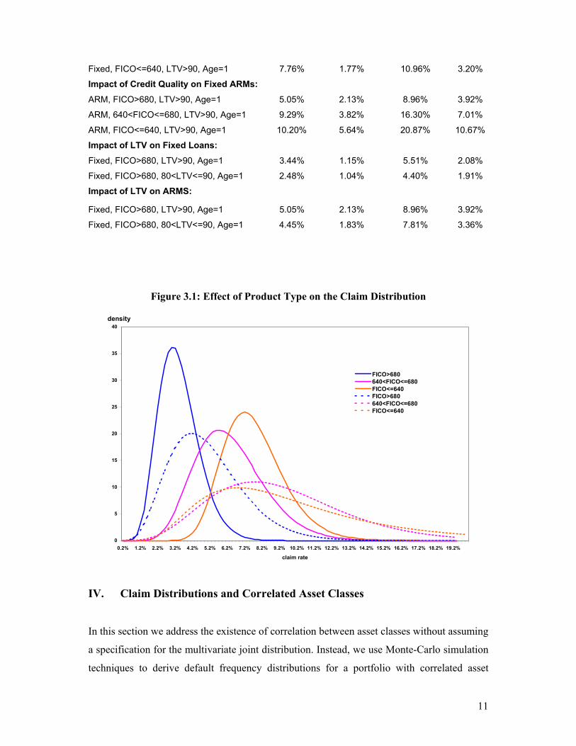
Figure 3.1 displays this difference in terms of the claim distribution between Fixed rate
mortgages and ARMs for newly originated loans with LTV>90. In this figure, the solid lines
represent fixed loans with the dotted loans denoting the ARM counterpart. This analysis
shows that the impact of lower credit quality on unexpected claims (UECR) increases
relatively faster for ARMs than for fixed loans. For the highest credit quality fixed loans, the
increase in UECR is 54% from 2.08% to 3.2%, while for ARMs this increase is nearly 173%.
While we observe the mean claim rate rise with lowered credit quality, the variance of the
sub-prime group for fixed loans actually decreases. As a result the UECR declines from
3.63% to 3.2% whereas in contrast, the ARMs variance increases to 5.64%. A similar type of
comparative statics may be performed on different LTV and age groups, but the overall
trends remain the same.
Table 3
Claim Rate Comparisons between Select Asset Classes
Asset Class Mean Std.Dev Q.995 UECR
Impact of Product Type:
Fixed, FICO>680, LTV>90, Age=1 3.44% 1.15% 5.51% 2.08%
ARM, FICO>680, LTV>90, Age=1 5.05% 2.13% 8.96% 3.92%
Fixed, FICO>680, 80<LTV<=90, Age=2 3.54% 1.24% 5.84% 2.30%
ARM, FICO>680, 80<LTV<=90, Age=2 6.27% 1.58% 9.08% 2.80%
Fixed, FICO<640, 80<LTV<=90, Age=2 7.33% 3.08% 13.11% 5.78%
ARM, FICO<640, 80<LTV<=90, Age=2 11.37% 3.01% 16.69% 5.32%
Impact of Credit Quality on Fixed Loans:
Fixed, FICO>680, LTV>90, Age=1 3.44% 1.15% 5.51% 2.08%
Fixed, 640<FICO<=680, LTV>90, Age=1 6.39% 2.01% 10.02% 3.63%
11
Fixed, FICO<=640, LTV>90, Age=1 7.76% 1.77% 10.96% 3.20%
Impact of Credit Quality on Fixed ARMs:
ARM, FICO>680, LTV>90, Age=1 5.05% 2.13% 8.96% 3.92%
ARM, 640<FICO<=680, LTV>90, Age=1 9.29% 3.82% 16.30% 7.01%
ARM, FICO<=640, LTV>90, Age=1 10.20% 5.64% 20.87% 10.67%
Impact of LTV on Fixed Loans:
Fixed, FICO>680, LTV>90, Age=1 3.44% 1.15% 5.51% 2.08%
Fixed, FICO>680, 80<LTV<=90, Age=1 2.48% 1.04% 4.40% 1.91%
Impact of LTV on ARMS:
Fixed, FICO>680, LTV>90, Age=1 5.05% 2.13% 8.96% 3.92%
Fixed, FICO>680, 80<LTV<=90, Age=1 4.45% 1.83% 7.81% 3.36%
Figure 3.1: Effect of Product Type on the Claim Distribution
IV. Claim Distributions and Correlated Asset Classes
In this section we address the existence of correlation between asset classes without assuming
a specification for the multivariate joint distribution. Instead, we use Monte-Carlo simulation
techniques to derive default frequency distributions for a portfolio with correlated asset
0
5
10
15
20
25
30
35
40
0.2% 1.2% 2.2% 3.2% 4.2% 5.2% 6.2% 7.2% 8.2% 9.2% 10.2% 11.2% 12.2% 13.2% 14.2% 15.2% 16.2% 17.2% 18.2% 19.2%
claim rate
density
FICO>680640<FICO<=680FICO<=640FICO>680640<FICO<=680FICO<=640

12
classes. We empirically show that an independence assumption underestimates the variance
of the distribution, which could result in undercapitalization for stress events. It is known that
from marginal probability distributions, it is generally infeasible to obtain the joint
distribution. Methods have been designed to address this issue given additional information
on the shape of the joint distribution, e.g. copula functions, a priori information and Bayesian
estimation methods. Our approach uses Monte-Carlo simulation with only information on the
covariance matrix, Cov(Xm)=Ωm, of m distinct asset classes where [x1, x2,…,xm]′=xm
represents a random draw. For notational purposes, we adhere to the convention where bold
capital letters refer to matrices, whereas bold lower case letters refer to vectors of a specific
size. In practice, covariance matrix Ωm is nearly always unknown to the analyst and must be
estimated. Frequently, because of limited data or non-stationary of parameters, the estimated
covariance matrix is not positive definite or a′ mΩ a <=0 ∀ a∈Rm. In this case, ridgeing
techniques or method of regularization estimators can be applied (Hoerl and Kennard, 1971;
van Akkeren, 2003). A more direct means of ensuring positive definiteness is possible by
addressing missing observations directly using hot deck imputation, mean substitution, or
regression methods.
To apply Monte-Carlo simulation, we use the estimated probability distribution
parameters on m-distinct asset classes
),(~),...,,(~),,(~),,(~ 223333
22222
21111 mmmm fxfxfxfx σµσµσµσµ (6)
, that are independent with covariance matrix diag([ 222
21 ,...,, mσσσ ]′)=Ξm and joint mean [µ1,
µ2,…, µm] ′= µm. In order to generate correlated pseudo-random samples from the above
distribution, we must find a function G:Rm→Rm such that G(xm) ~ (µm, mΩ ). Let function G
be of linear form:
G(xm)=Axm+bm (7)
, where A is an (m ∗ m) matrix and bm is an m-dimensional vector. We first transform xm
such that Cov(f(xm))=Im, or ym= Ξm-1/2 xm ~ (Ξm
-1/2 µm, I). Taking expectations of both sides of
equation (7) allows us to obtain:
E[G(ym)]=A Ξm-1/2 µm +bm= µm (8)

13
Cov[G(xm)]=AA′ = mΩ (9)
, from which the unknowns A and bm are obtained as
A = 2/1mΩ (10)
bm= (I – A Ξm-1/2) µm. (11)
Equations (10) and (11) exist because of the positive definiteness of mΩ .
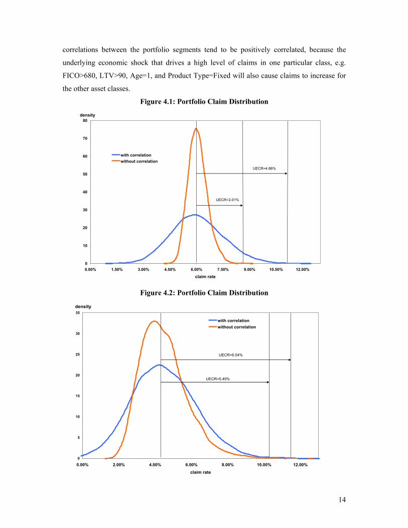
Figures 4.1 and 4.2 show two examples of portfolio claim distributions estimated with
and without correlation effects. The first figure shows a larger set of loans spanning a wider
range of credit quality and across all 72-asset classes. As explained in the above derivations,
the estimated claim rate will equal wm′µm for estimation with and without correlated effects.
Here wm=[w1, w2,…,wm]′ represents the set of weights on each asset class. The figures clearly
indicate underestimation of right hand tail probabilities when correlation is not incorporated.
More precisely, the unexpected claim rate (UECR) in Figure 4.1 as measured by the 99.9% of
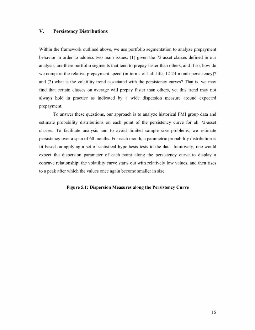
the distribution increases by 2.85% from 2.01% to 4.86%. In Figure 4.2, the expected claim
rate is much lower than that of portfolio 1 driven by less exposure to products with higher
expected claim rates, such as ARMS and higher average credit quality (FICO scores).
However, while the expected claim rate decreases noticeably from 6% to 4.4% in Figure 4.2,
increased variability of the portfolio distribution causes the unexpected claim rate to jump to
5.49% and 6.04%. This analysis implies that if correlation effects are not properly estimated
and incorporated in the joint distribution, the amount of capital set aside to cover such a
downturn scenario will be inadequate.
The variance of the portfolio distribution, Var[wm′xm], is strictly positive, ensured by
the positive definiteness property of the covariance matrix. Therefore, the portfolio variance
is determined by the set of weights, wm, and the estimated covariance matrix mΩ . The
condition that the variance of a portfolio with correlated asset classes exceeds the variance of
the portfolio without correlation does not need to hold theoretically. This can be illustrated
from a 2 asset class example where the variance under independence, 22
22
21
21 σσ ww + , is larger
than the variance calculated under correlated asset classes, 122122
22
21
21 2 σσσ wwww ++ , if the
asset classes are negatively correlated. When estimating claim distributions in general,
14
correlations between the portfolio segments tend to be positively correlated, because the
underlying economic shock that drives a high level of claims in one particular class, e.g.
FICO>680, LTV>90, Age=1, and Product Type=Fixed will also cause claims to increase for
the other asset classes.
Figure 4.1: Portfolio Claim Distribution
0
10
20
30
40
50
60
70
80
0.00% 1.50% 3.00% 4.50% 6.00% 7.50% 9.00% 10.50% 12.00%
claim rate
density
with correlationwithout correlation
UECR=4.86%
UECR=2.01%
Figure 4.2: Portfolio Claim Distribution
0
5
10
15
20
25
30
35
0.00% 2.00% 4.00% 6.00% 8.00% 10.00% 12.00%
claim rate
density
with correlationwithout correlation
UECR=5.49%
UECR=6.04%
15
V. Persistency Distributions
Within the framework outlined above, we use portfolio segmentation to analyze prepayment
behavior in order to address two main issues: (1) given the 72-asset classes defined in our
analysis, are there portfolio segments that tend to prepay faster than others, and if so, how do
we compare the relative prepayment speed (in terms of half-life, 12-24 month persistency)?
and (2) what is the volatility trend associated with the persistency curves? That is, we may
find that certain classes on average will prepay faster than others, yet this trend may not
always hold in practice as indicated by a wide dispersion measure around expected
prepayment.
To answer these questions, our approach is to analyze historical PMI group data and
estimate probability distributions on each point of the persistency curve for all 72-asset
classes. To facilitate analysis and to avoid limited sample size problems, we estimate
persistency over a span of 60 months. For each month, a parametric probability distribution is
fit based on applying a set of statistical hypothesis tests to the data. Intuitively, one would
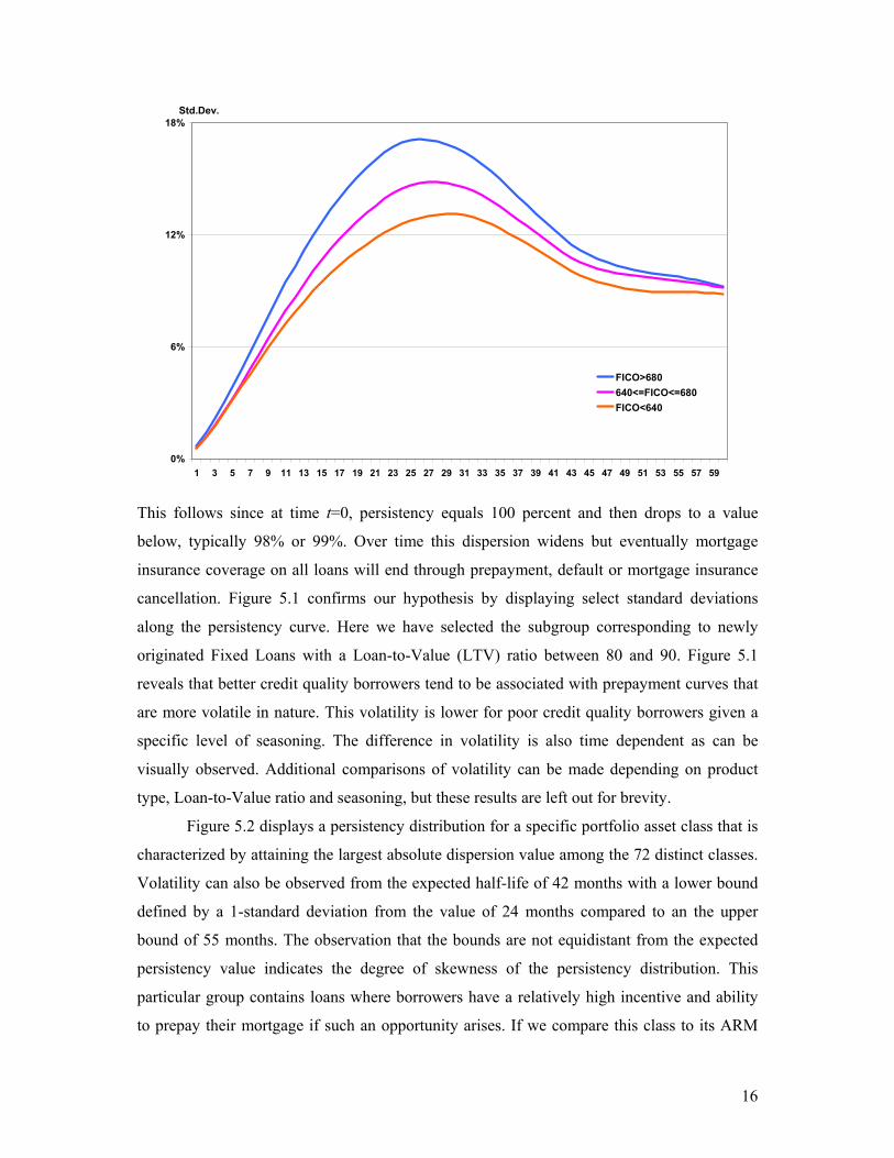
expect the dispersion parameter of each point along the persistency curve to display a
concave relationship: the volatility curve starts out with relatively low values, and then rises
to a peak after which the values once again become smaller in size.
Figure 5.1: Dispersion Measures along the Persistency Curve
16
0%
6%
12%
18%
1 3 5 7 9 11 13 15 17 19 21 23 25 27 29 31 33 35 37 39 41 43 45 47 49 51 53 55 57 59
Std.Dev.
FICO>680640<=FICO<=680FICO<640
This follows since at time t=0, persistency equals 100 percent and then drops to a value
below, typically 98% or 99%. Over time this dispersion widens but eventually mortgage
insurance coverage on all loans will end through prepayment, default or mortgage insurance
cancellation. Figure 5.1 confirms our hypothesis by displaying select standard deviations
along the persistency curve. Here we have selected the subgroup corresponding to newly
originated Fixed Loans with a Loan-to-Value (LTV) ratio between 80 and 90. Figure 5.1
reveals that better credit quality borrowers tend to be associated with prepayment curves that
are more volatile in nature. This volatility is lower for poor credit quality borrowers given a
specific level of seasoning. The difference in volatility is also time dependent as can be
visually observed. Additional comparisons of volatility can be made depending on product
type, Loan-to-Value ratio and seasoning, but these results are left out for brevity.
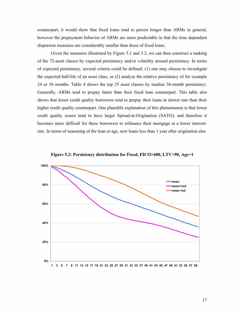
Figure 5.2 displays a persistency distribution for a specific portfolio asset class that is
characterized by attaining the largest absolute dispersion value among the 72 distinct classes.
Volatility can also be observed from the expected half-life of 42 months with a lower bound
defined by a 1-standard deviation from the value of 24 months compared to an the upper
bound of 55 months. The observation that the bounds are not equidistant from the expected
persistency value indicates the degree of skewness of the persistency distribution. This
particular group contains loans where borrowers have a relatively high incentive and ability
to prepay their mortgage if such an opportunity arises. If we compare this class to its ARM
17
counterpart, it would show that fixed loans tend to persist longer than ARMs in general,
however the prepayment behavior of ARMs are more predictable in that the time dependent
dispersion measures are considerably smaller than those of fixed loans.
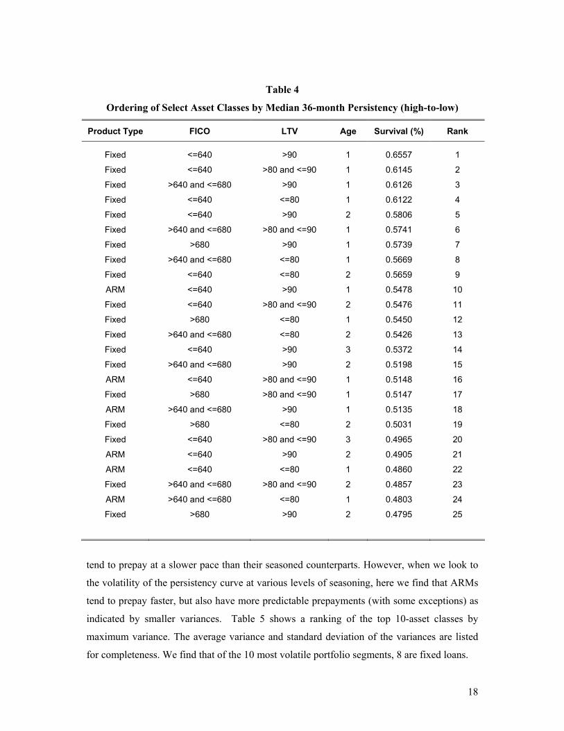
Given the measures illustrated by Figure 5.1 and 5.2, we can then construct a ranking
of the 72-asset classes by expected persistency and/or volatility around persistency. In terms
of expected persistency, several criteria could be defined: (1) one may choose to investigate
the expected half-life of an asset class, or (2) analyze the relative persistency of for example
24 or 36 months. Table 4 shows the top 25 asset classes by median 36-month persistency.
Generally, ARMs tend to prepay faster than their fixed loan counterpart. This table also
shows that lesser credit quality borrowers tend to prepay their loans at slower rate than their
higher credit quality counterpart. One plausible explanation of this phenomenon is that lower
credit quality scores tend to have larger Spread-at-Origination (SATO), and therefore it
becomes more difficult for these borrowers to refinance their mortgage at a lower interest-
rate. In terms of seasoning of the loan or age, new loans less than 1 year after origination also
Figure 5.2: Persistency distribution for Fixed, FICO>680, LTV>90, Age=1
0%
20%
40%
60%
80%
100%
1 3 5 7 9 11 13 15 17 19 21 23 25 27 29 31 33 35 37 39 41 43 45 47 49 51 53 55 57 59
meanmean+1sdmean-1sd
18
Table 4
Ordering of Select Asset Classes by Median 36-month Persistency (high-to-low)
Product Type FICO LTV Age Survival (%) Rank
Fixed <=640 >90 1 0.6557 1
Fixed <=640 >80 and <=90 1 0.6145 2
Fixed >640 and <=680 >90 1 0.6126 3
Fixed <=640 <=80 1 0.6122 4
Fixed <=640 >90 2 0.5806 5
Fixed >640 and <=680 >80 and <=90 1 0.5741 6
Fixed >680 >90 1 0.5739 7
Fixed >640 and <=680 <=80 1 0.5669 8
Fixed <=640 <=80 2 0.5659 9
ARM <=640 >90 1 0.5478 10
Fixed <=640 >80 and <=90 2 0.5476 11
Fixed >680 <=80 1 0.5450 12
Fixed >640 and <=680 <=80 2 0.5426 13
Fixed <=640 >90 3 0.5372 14
Fixed >640 and <=680 >90 2 0.5198 15
ARM <=640 >80 and <=90 1 0.5148 16
Fixed >680 >80 and <=90 1 0.5147 17
ARM >640 and <=680 >90 1 0.5135 18
Fixed >680 <=80 2 0.5031 19
Fixed <=640 >80 and <=90 3 0.4965 20
ARM <=640 >90 2 0.4905 21
ARM <=640 <=80 1 0.4860 22
Fixed >640 and <=680 >80 and <=90 2 0.4857 23
ARM >640 and <=680 <=80 1 0.4803 24
Fixed >680 >90 2 0.4795 25
tend to prepay at a slower pace than their seasoned counterparts. However, when we look to
the volatility of the persistency curve at various levels of seasoning, here we find that ARMs
tend to prepay faster, but also have more predictable prepayments (with some exceptions) as
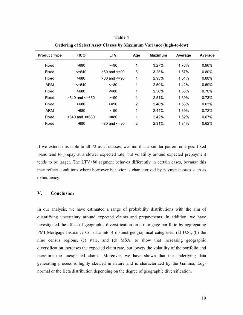
indicated by smaller variances. Table 5 shows a ranking of the top 10-asset classes by
maximum variance. The average variance and standard deviation of the variances are listed
for completeness. We find that of the 10 most volatile portfolio segments, 8 are fixed loans.
19
Table 4
Ordering of Select Asset Classes by Maximum Variance (high-to-low)
Product Type FICO LTV Age Maximum Average Average
Fixed >680 >=90 1 3.27% 1.76% 0.96%
Fixed <=640 >80 and <=90 3 3.25% 1.57% 0.80%
Fixed >680 >80 and <=90 1 2.93% 1.51% 0.88%
ARM <=640 <=80 1 2.59% 1.42% 0.69%
Fixed >680 <=80 1 2.56% 1.58% 0.70%
Fixed >640 and <=680 >=90 1 2.51% 1.39% 0.73%
Fixed >680 >=90 2 2.48% 1.53% 0.63%
ARM >680 >=90 1 2.44% 1.39% 0.72%
Fixed >640 and <=680 <=80 1 2.42% 1.52% 0.67%
Fixed >680 >80 and <=90 2 2.31% 1.34% 0.62%
If we extend this table to all 72 asset classes, we find that a similar pattern emerges: fixed
loans tend to prepay at a slower expected rate, but volatility around expected prepayment
tends to be larger. The LTV<80 segment behaves differently in certain cases, because this
may reflect conditions where borrower behavior is characterized by payment issues such as
delinquency.
V. Conclusion
In our analysis, we have estimated a range of probability distributions with the aim of
quantifying uncertainty around expected claims and prepayments. In addition, we have
investigated the effect of geographic diversification on a mortgage portfolio by aggregating
PMI Mortgage Insurance Co. data into 4 distinct geographical categories: (a) U.S., (b) the
nine census regions, (c) state, and (d) MSA, to show that increasing geographic
diversification increases the expected claim rate, but lowers the volatility of the portfolio and
therefore the unexpected claims. Moreover, we have shown that the underlying data
generating process is highly skewed in nature and is characterized by the Gamma, Log-
normal or the Beta distribution depending on the degree of geographic diversification.
20
Segmenting the portfolio into distinct homogeneous asset segments allows for the
estimation of risk under correlated asset classes. In the case of U.S. residential mortgages, we
identify a set of classes that incorporates: (a) mortgage product type, (b) credit quality
segmentation, (c) LTV, and (d) seasoning. Our approach then uses Monte-Carlo simulation
with information on the estimated covariance matrix and the underlying skewed probability
distributions to estimate the portfolio claim distribution. Empirically, it is shown in 2
examples that the variance of a portfolio in the case of correlated asset classes is larger than
when independence is assumed. Local economic conditions are an important driver of
variation in claim rates and affect all portfolio segments to a certain extent. A portfolio with
correlated asset classes therefore generally displays more volatility than a portfolio with
independent asset classes.
Portfolio segmentation is also used to analyze prepayment behavior in order to assess
whether there are classes that tend to prepay faster than others, but also whether certain
classes display more volatility than others. That is, we may find that specific portfolio
segments on average will prepay faster than others, yet this trend may not always hold in
practice as indicated by a wide dispersion measure around expected prepayment. Our results
suggest than on average, fixed mortgages tend to persist longer than ARMs, however ARMs
are less volatile in that the variance around expected persistency tends to be smaller. A
ranking can be devised that orders portfolio classes by expected persistency and/or volatility
around this expectation.
With regards to future analysis and research direction, the application of mixture
distributions appears to be a promising area for additional work. A Log-normal-beta
distribution may empirically fit the data better than the Log-normal or the Beta distribution
by itself and a future study may investigate the optimal combinations of distributions. In
terms of the statistical estimation techniques, a comparison between information recovery
rules could potentially shed some light on when procedures empirically are more desirable
than others. That is, do moment based estimators tend to yield smaller tail probabilities than
likelihood based procedures, and are their alternative information recovery rules than could
provide an advantage? Bayesian estimation procedures have shown to be successful in the
estimation of skewed distributions when theoretically one could expect a high claim rate
which however has not been observed empirically due to limitations of the data. Finally, a
factor based duration model could statistically provide a means of more accurately measuring
claim development over time. This technique would allow for the introduction of external
covariates and could potentially use Monte-Carlo simulation as a means to quantify volatility.

21
REFERENCES
Crouhy, M., Galia, D. and Mark, R. (2001). Risk Management. McGraw-Hill. New York, NY.
Duffie, D. and Singleton, K. (2003). Credit Risk. Princeton University Press. Princeton, NJ.
Hayre, L. (2001). Salomon Smith Barney Guide to Mortgage-Backed and Asset-Backed
Securities. John Wiley & Sons, Inc. New York, NY.
Hoerl, A. and Kennard, R. (1970) Ridge Regression: Biased estimation for nonorthogonal
problems. Technometrics, 12, 55-67.
Holton, G. (2003). Value-at-Risk: Theory and Practice. Academic Press, New York, NY.
Nakada, P., Shah, H., Koyluoglu, H. and Collignon, O. (1999). P&C Raroc: A Catalyst for
Improved Capital Management in the Property and Casualty Insurance Industry. The Journal
of Risk Finance, fall, 1-18.
Rice, J. (1995). Mathematical Statistics and Data Analysis. Duxbury Press, Belmont, CA.
Van Akkeren, M. (2003) An Information Theoretic Approach to Estimation in the Case of
Multicollinearity. Computational Economics, 22, 1-22.
Zaik, E., Walter, J. and Kelling, G. (1996). RAROC at the Bank of America: from Theory to
Practice. Journal of Applied Corporate Finance, 6(3), 85-93.