Bayesian Multivariate Isotonic Regression Splines:

Applications to Carcinogenicity Studies

Bo Cai and David B. Dunson∗

Biostatistics Branch, National Institute of Environmental Health Sciences,

P.O. Box 12233, Research Triangle Park, NC 27709, U.S.A.

∗dunson1@niehs.nih.gov

In many applications, interest focuses on assessing the relationship between a predictor and

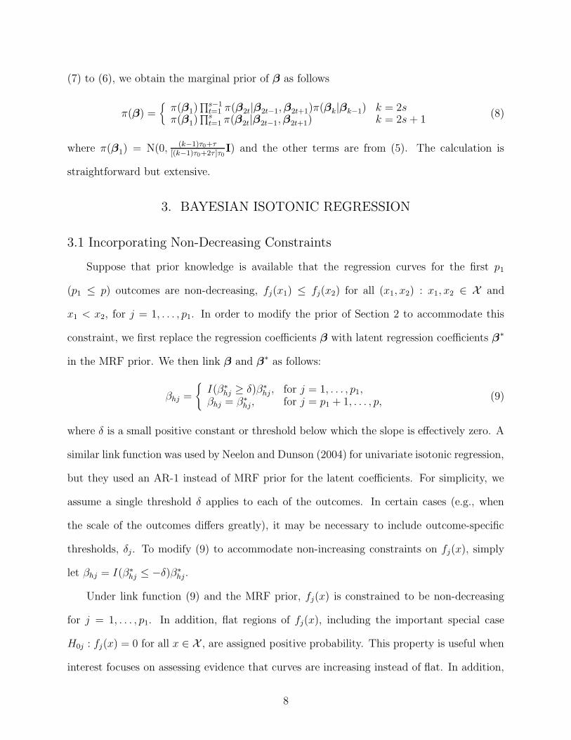
a multivariate outcome variable, and there may be prior knowledge about the shape of the

regression curves. For example, regression functions relating dose of a possible risk factor to

different adverse outcomes can often be assumed to be nondecreasing. In such cases, interest

focuses on (1) assessing evidence of an overall adverse effect; (2) determining which outcomes

are most affected; and (3) estimating outcome-specific regression curves. This article pro-

poses a Bayesian approach for addressing this problem, motivated by multi-site tumor data

from carcinogenicity experiments. A multivariate smoothing spline model is specified, which

accommodates dependency in the multiple curves through a hierarchical Markov random

field prior for the basis coefficients, while also allowing for residual correlation. A Gibbs

sampler is proposed for posterior computation, and the approach is applied to data on body

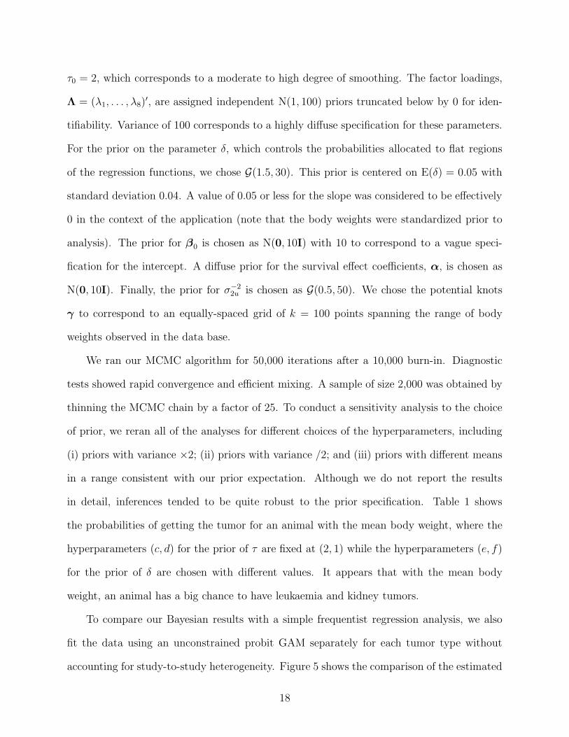
weight and tumor occurrence.

KEY WORDS: Factor model; Functional data analysis; Monotone curves; Multiple out-

comes; Multiplicity problem; Seemingly unrelated regression; Smoothing; Tumor data.

1

1. INTRODUCTION

1.1 Background and Motivation

In many applications, data are collected for multiple outcome variables and interest focuses

on assessing the functional relationship between a continuous predictor and the mean, ad-

justing for covariates. In such cases, it is common to have prior knowledge of the direction

of the regression functions for one or more of the outcome variables. For example, if the

predictor is dose of a potentially adverse exposure, then dose response curves should be non-

decreasing for adverse responses, at least after adjusting for important confounding variables.

It is well known that incorporating such constraints, when justified, can improve estimation

efficiency and power to detect associations (Robertson, Wright and Dykstra, 1988). When

outcome data are multivariate, it becomes necessary to not only flexibly model the indi-

vidual regression functions subject to the non-decreasing constraint but also to characterize

dependency.

The problem of flexible nonlinear regression modeling of multiple response data has

been the focus of a growing body of literature. Much of the literature has focused on data

consisting of repeated observations over time (Brumback and Rice, 1998; Staniswalis and Lee,

1998; Wu and Zhang, 2002, among many others). In the case where data are multivariate

normal and the regression functions are expressed as weighted sums of a common set of basis

functions, many of the univariate methods generalize directly to the multivariate case (Brown

et al., 1998). The literature on seemingly unrelated regressions (SUR) (Zellner, 1962) focuses

on the more general case where the basis functions vary for the different outcomes, and the

regressions are related through residual correlation (refer to Ng, 2002 and Holmes, Denison,

and Mallick, 2002 for recent references). None of these articles considered the incorporation

of monotonicity constraints.

For univariate data, a number of approaches have been proposed for frequentist (Mam-

2

men, 1991; Lee, 1996; Ramsay, 1998) and Bayesian (Lavine and Mockus, 1995; Schmid

and Brown, 1999; Holmes and Heard, 2003; Neelon and Dunson, 2004) monotone curve

estimation. Our interest is in developing a Bayesian framework for joint estimation and

inferences on smooth non-decreasing regression curves for multiple categorical and continu-

ous outcomes. In many applications, interest focuses on not only estimating the regression

functions but also assessing evidence of overall increasing trends and the locations of flat

regions.

1.2 Application: Body Weight and Tumor Occurrence

Our focus is on assessing the relationship between body weight and the occurrence of tumors

in different organ sites using data from the National Toxicology Program (NTP) historical

control data base. Previous analyses of NTP data have shown evidence of a positive as-

sociation between body weight at one year of age and the incidence of tumors in certain

sites (Seilkop, 1995; Haseman et al., 1997; Parise et al., 2001). Parise et al. (2001) used

a semiparametric logistic mixed effects model with a random intercept for study to relate

52 week body weight to the probability of tumor development. They implemented sepa-

rate analyses for the different tumor sites instead of considering them jointly, and did not

consider the incorporation of an order constraint on the curve. Our interest is in jointly

modeling the body weight effect on the incidence of the eight most common tumors, includ-

ing leukaemia, pheochromocytomas, pituitary, mammary, thyroid, subcutaneous, pancreas,

and kidney tumors, focusing on male rats for sake of brevity.

Following previous authors in assuming that tumors are unlikely to have progressed to a

stage causing morbidity by one year of age (at least in control animals), it is anticipated that

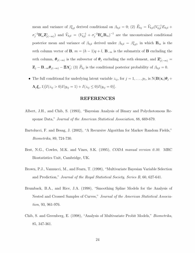
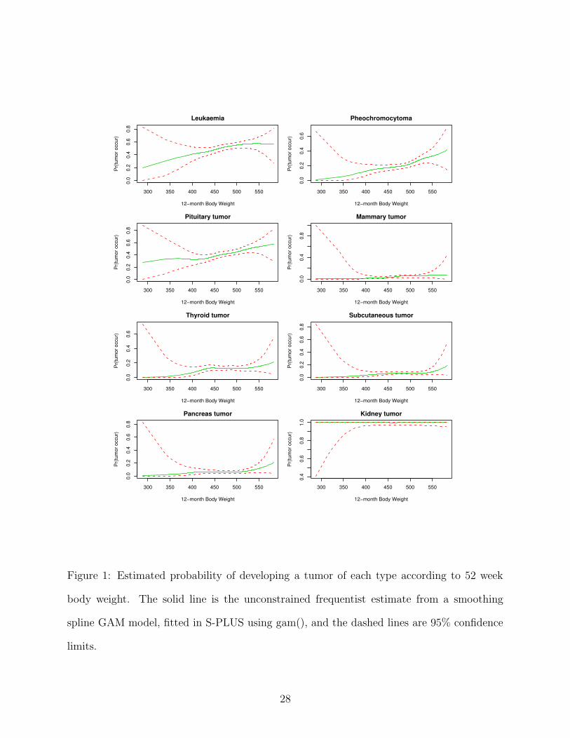
tumor incidence is non-decreasing with 52 week body weight, adjusting for animal survival.

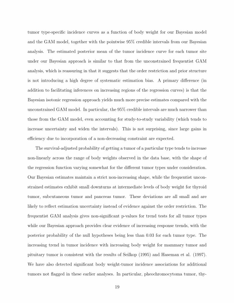
Our priliminary analysis shown in Figure 1 also confirms the non-decreasing constraint as-

sumption. However, it is not known which tumor types are sensitive to body weight, and an

3

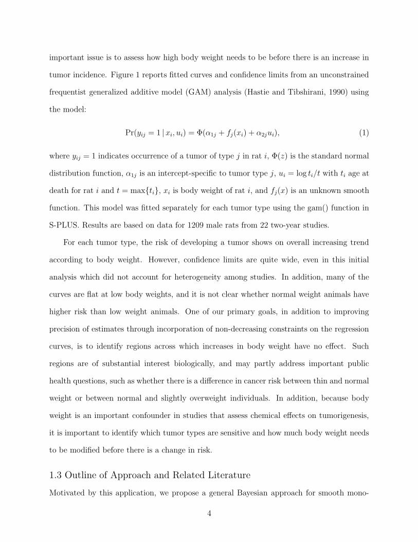
important issue is to assess how high body weight needs to be before there is an increase in

tumor incidence. Figure 1 reports fitted curves and confidence limits from an unconstrained

frequentist generalized additive model (GAM) analysis (Hastie and Tibshirani, 1990) using

the model:

Pr(yij = 1 | xi, ui) = Φ(α1j + fj(xi) + α2jui), (1)

where yij = 1 indicates occurrence of a tumor of type j in rat i, Φ(z) is the standard normal

distribution function, α1j is an intercept-specific to tumor type j, ui = log ti/t with ti age at

death for rat i and t = max{ti}, xi is body weight of rat i, and fj(x) is an unknown smooth

function. This model was fitted separately for each tumor type using the gam() function in

S-PLUS. Results are based on data for 1209 male rats from 22 two-year studies.

For each tumor type, the risk of developing a tumor shows on overall increasing trend

according to body weight. However, confidence limits are quite wide, even in this initial

analysis which did not account for heterogeneity among studies. In addition, many of the

curves are flat at low body weights, and it is not clear whether normal weight animals have

higher risk than low weight animals. One of our primary goals, in addition to improving

precision of estimates through incorporation of non-decreasing constraints on the regression

curves, is to identify regions across which increases in body weight have no effect. Such

regions are of substantial interest biologically, and may partly address important public

health questions, such as whether there is a difference in cancer risk between thin and normal

weight or between normal and slightly overweight individuals. In addition, because body

weight is an important confounder in studies that assess chemical effects on tumorigenesis,

it is important to identify which tumor types are sensitive and how much body weight needs

to be modified before there is a change in risk.

1.3 Outline of Approach and Related Literature

Motivated by this application, we propose a general Bayesian approach for smooth mono-

4

tone curve estimation and inferences for multiple outcome data. In particular, we describe

a general multivariate isotonic regression factor model for binary outcomes. This approach

has some conceptual relationship to the method of Neelon and Dunson (2004), which was

developed for univariate isotonic regression. However, motivated by the body weight-tumor

incidence application, we propose a different model, prior structure, and computational algo-

rithm, which accommodates multivariate outcome data and allows for study-to-study vari-

ability. The model is related to multivariate probit models with a semiparametric isotonic

regression structure for the mean and with a hierarchical factor analytic covariance structure.

We follow the strategy of Albert and Chib (1993) in introducing latent variables to facili-

tate posterior computation via a data augmentation Markov chain Monte Carlo (MCMC)

algorithm. The factor analytic structure can be chosen motivated by the carcinogenicity

application to reduce dimensionality of the covariance matrix relative to the model of Chib

and Greenberg (1998).

In Section 2 we discuss the regression model for multiple outcomes and the prior struc-

ture for regression coefficients. In Sections 3 and 4, we propose the multivariate isotonic

regression model and approach to posterior computation. In Section 5 we describe the mul-

tivariate isotonic regression factor model for binary outcomes and the algorithm for posterior

computation. In Section 6, we present a simulation study. In Section 7 we apply the ap-

proach to the NTP data on body weight and tumor occurrence. In Section 8 we summarize

and discuss the results.

2. REGRESSION SPLINES FOR MULTIPLE OUTCOMES

Interest focuses on assessing the relationship between a predictor xi and a multivariate

outcome yi = (yi1, . . . , yip)′, with data collected for subjects i = 1, . . . , n. We initially

assume that yi has a multivariate normal distribution with xi the only predictor:

yi ∼ Np(µ(xi),Σ), (2)

5

where µ(x) = [f1(x), . . . , fp(x)]′ is a vector of unknown regression functions specific to out-

comes 1, . . . , p, respectively, Σ is a covariance matrix, and xi ∈ X = [γ0, γk]. Generalizations

to allow multiple predictors and binary outcomes will be described in Section 5.

We assume that each curve can be characterized as a linear combination of a common

set of potential basis functions so that

fj(xi) = β0j +k∑

h=1

βhjBh(xi), for j = 1, . . . , p, (3)

where β0j is an intercept for outcome j, and βhj is a regression coefficient for outcome j and

basis function Bh(x). In particular, we will focus on the regression spline basis functions:

Bh(xi) = I(xi > γh−1)[ min(xi, γh) − γh−1]m, (4)

where γ = (γ1, . . . , γk)′ are potential knot points with γ0 < γ1 < . . . < γk, and m gives the

order of the spline. We focus on linear splines having m = 1 but the methods generalize

directly.

Although we assume a common set of potential basis functions for the different outcomes,

the effective number of basis functions can vary since our isotonic regression prior (to be

described in Section 3) allows flat regions across which the regression coefficients are constant.

The locations of these flat regions can vary for the different outcomes. Markov random field

(MRF) formulations originated in spatial statistics and play a central role in the areas such

as random graphs, graphical models and statistical physics. To define an MRF, one can

specify conditional distributions for each of the elements of a random vector to depend only

on neighboring elements. In our case, initially focusing on the unconstrained case, we define

an MRF-type prior

π(βh |βh−1,βh+1)d=

Np

((τ

τ0+τ

)β2, (τ0 + τ)−1

Ip

)h = 1

Np

(0.5(βh−1 + βh+1), 0.5τ

−1Ip

)h = 2, . . . , k − 1

Np

((τ

τ0+τ

)βk−1, (τ0 + τ)−1

Ip

)h = k

(5)

Under expression (4) with m = 1, the elements of βh = (βh1, . . . , βhp)′, h = 1, . . . , k, are

interpretable as local slopes within interval (γh−1, γh] for outcomes j = 1, . . . , p. The MRF

6

prior centers βh on its nearest neighbors, βh−1 and βh+1. In the interior bins (h = 2, . . . , k−

1), the prior expection of βh is simply an average of the slopes in the adjacent bins, with

the precision depending on the smoothing parameter τ . In the exterior bins (h = 1, k), the

conditional prior for βh is proportional to the product of a Np(βh; 0, τ−10 Ip) density and a Np

density centered on the slopes in the adjacent interior bin. This MRF structure allows the

interval-specific slopes to be updated by borrowing the information from their neighbors. It

also centers the MRF prior for the interval-specific slopes on 0 and smoothes the local slopes

across X to a degree depending on τ . In the limiting case as τ → ∞, βh is constant for

h = 1, . . . , k, and the model reduces to a multiple linear regression model.

One motivation for using this particular MRF structure is that it ensures that the prior

variance is the same at both endpoints of X . As noted by Denison et al.(2002), the most

reasonable default choice in the absence of additional information is to assume equal prior

variance at the endpoints. We describe a generalization of this prior to accommodate mono-

tonicity constraints on the regression functions in the next section.

To compute the posterior distribution of β = (β′

1, . . . ,β′

k)′ defined above, it is necessary

to find the prior expression of β, i.e. π(β). We note that the following expression holds:

π(β) = π(β1)k∏

h=2

π(βh|β<h), (6)

where β<h = {βj : j < h}. However, the product terms above are not easily obtained.

We adopt the recursive algorithm proposed by Bartolucci and Besag (2002) by which the

individual terms of (6) can be evaluated as full conditionals of βh obtained by marginalising

over β>h. According to Theorem 1 from Bartolucci and Besag (2002), we can calculate the

elements of (6) recursively

π(βh|β<h) =[ ∫

π(βh+1|β<h+1)

π(βh|βh−1,βh+1)dβh+1

]−1, h = 1, . . . , k − 1 (7)

Clearly, π(β1|β<1) = π(β1) and π(βk|β<k) = π(βk|βk−1). By substituting the results from

7

(7) to (6), we obtain the marginal prior of β as follows

π(β) ={π(β1)

∏s−1t=1 π(β2t|β2t−1,β2t+1)π(βk|βk−1) k = 2s

π(β1)∏s

t=1 π(β2t|β2t−1,β2t+1) k = 2s+ 1(8)

where π(β1) = N(0, (k−1)τ0+τ

[(k−1)τ0+2τ ]τ0I) and the other terms are from (5). The calculation is

straightforward but extensive.

3. BAYESIAN ISOTONIC REGRESSION

3.1 Incorporating Non-Decreasing Constraints

Suppose that prior knowledge is available that the regression curves for the first p1

(p1 ≤ p) outcomes are non-decreasing, fj(x1) ≤ fj(x2) for all (x1, x2) : x1, x2 ∈ X and

x1 < x2, for j = 1, . . . , p1. In order to modify the prior of Section 2 to accommodate this

constraint, we first replace the regression coefficients β with latent regression coefficients β∗

in the MRF prior. We then link β and β∗ as follows:

βhj =

{I(β∗

hj ≥ δ)β∗

hj, for j = 1, . . . , p1,βhj = β∗

hj, for j = p1 + 1, . . . , p, (9)

where δ is a small positive constant or threshold below which the slope is effectively zero. A

similar link function was used by Neelon and Dunson (2004) for univariate isotonic regression,

but they used an AR-1 instead of MRF prior for the latent coefficients. For simplicity, we

assume a single threshold δ applies to each of the outcomes. In certain cases (e.g., when

the scale of the outcomes differs greatly), it may be necessary to include outcome-specific

thresholds, δj. To modify (9) to accommodate non-increasing constraints on fj(x), simply

let βhj = I(β∗

hj ≤ −δ)β∗

hj.

Under link function (9) and the MRF prior, fj(x) is constrained to be non-decreasing

for j = 1, . . . , p1. In addition, flat regions of fj(x), including the important special case

H0j : fj(x) = 0 for all x ∈ X , are assigned positive probability. This property is useful when

interest focuses on assessing evidence that curves are increasing instead of flat. In addition,

8

by placing mass on the boundary, we obtain a shrinkage estimator of the regression function.

Since the result of James and Stein (1961), shrinkage estimates have been shown to have

good properties in many cases. In simulation examples, our estimator has exhibited lower

risk under squared error loss compared with the corresponding unconstrained estimator for

a variety of cases, though uniform domination results are not yet available.

3.2 Hierarchical Covariance Structure and Prior Specification

To complete a Bayesian specification of our model, we need to choose prior distributions

for the residual covariance Σ, intercept parameters β0 = (β01, . . . , β0p)′, knots γ, smoothing

parameter τ , and the threshold δ. We assume a priori independence for these different

parameter vectors and let

π(β0) = Np(β0; 0, sIp), π(Σ) = IW(Σ; v,R−1), π(τ) = G(τ ; c, d), π(δ) = G(δ; e, f), (10)

where IW(·) denotes the inverse-Wishart density, and s, v,R, c, d, e, f are investigator-

specified hyperparameters. With the exception of π(δ), these priors are conditionally-

conjugate. Issues in choosing these hyperparameters will be discussed in Section 5.

We follow a related approach to Smith and Kohn (1996) and Neelon and Dunson (2004)

in choosing a prior for the knots based on selecting from a large number of prespecified

potential knot locations (e.g., the unique values of the predictor). In particular, letting γ

denote this prespecified vector of knots, our prior for β effectively allows knots to drop out

of the model by allowing for flat regions of the regression functions.

4. POSTERIOR COMPUTATION

For posterior computation, we propose a hybrid Gibbs-Metropolis algorithm which alternates

between the following steps: (1) update τ from its full conditional distribution by using

rejection sampling; (2) update Σ from its inverse-Wishart full conditional distribution; (3)

update the intercept parameters β0j from normal full conditional distributions; and (4)

9

update δ and (βhj, β∗

hj) in a block by sampling a candidate for δ and drawing the β’s from

their full conditional distributions.

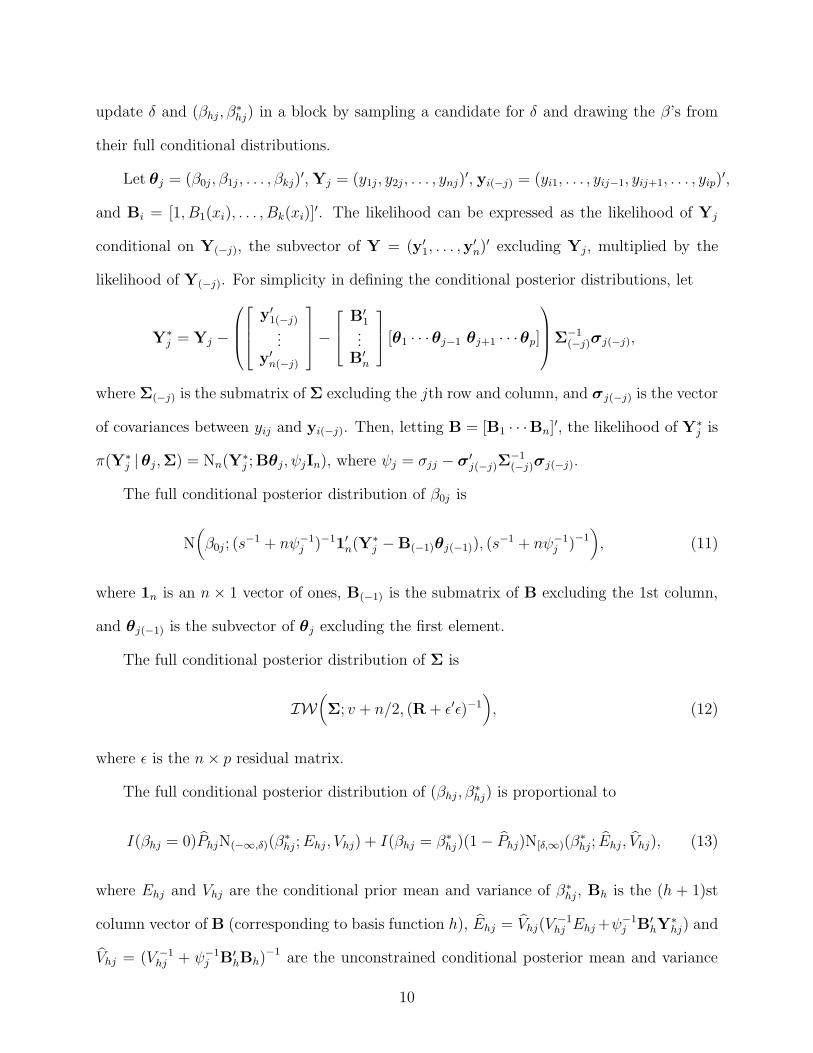
Let θj = (β0j, β1j , . . . , βkj)′, Yj = (y1j, y2j, . . . , ynj)

′, yi(−j) = (yi1, . . . , yij−1, yij+1, . . . , yip)′,

and Bi = [1, B1(xi), . . . , Bk(xi)]′. The likelihood can be expressed as the likelihood of Yj

conditional on Y(−j), the subvector of Y = (y′

1, . . . ,y′

n)′ excluding Yj, multiplied by the

likelihood of Y(−j). For simplicity in defining the conditional posterior distributions, let

Y∗

j = Yj −

y′

1(−j)...

y′

n(−j)

−

B′

1...

B′

n

[θ1 · · ·θj−1 θj+1 · · ·θp]

Σ−1

(−j)σj(−j),

where Σ(−j) is the submatrix of Σ excluding the jth row and column, and σj(−j) is the vector

of covariances between yij and yi(−j). Then, letting B = [B1 · · ·Bn]′, the likelihood of Y∗

j is

π(Y∗

j | θj,Σ) = Nn(Y∗

j ;Bθj, ψjIn), where ψj = σjj − σ′

j(−j)Σ−1(−j)σj(−j).

The full conditional posterior distribution of β0j is

N(β0j ; (s

−1 + nψ−1j )−11′

n(Y∗

j − B(−1)θj(−1)), (s−1 + nψ−1

j )−1), (11)

where 1n is an n× 1 vector of ones, B(−1) is the submatrix of B excluding the 1st column,

and θj(−1) is the subvector of θj excluding the first element.

The full conditional posterior distribution of Σ is

IW(Σ; v + n/2, (R + ε′ε)−1

), (12)

where ε is the n× p residual matrix.

The full conditional posterior distribution of (βhj, β∗

hj) is proportional to

I(βhj = 0)PhjN(−∞,δ)(β∗

hj;Ehj, Vhj) + I(βhj = β∗

hj)(1 − Phj)N[δ,∞)(β∗

hj; Ehj, Vhj), (13)

where Ehj and Vhj are the conditional prior mean and variance of β∗

hj, Bh is the (h + 1)st

column vector of B (corresponding to basis function h), Ehj = Vhj(V−1hj Ehj +ψ

−1j B′

hY∗

hj) and

Vhj = (V −1hj + ψ−1

j B′

hBh)−1 are the unconstrained conditional posterior mean and variance

10

of βhj derived under βhj = β∗

hj, Y∗

hj = Y∗

j − Bθj + Bhβ∗

hj, and the conditional posterior

probability of βhj = 0 is

Phj =

[1 +

Φ(−δ; Ehj, Vhj)N(0;Ehj, Vhj)

Φ(δ;Ehj, Vhj)N(0; Ehj, Vhj)

]−1

.

Hence, the full conditional posterior distribution of (βhj, β∗

hj) is a mixture of two truncated

normal distributions, which is straightforward to sample from.

5. FACTOR MODELS FOR MULTIPLE BINARY OUTCOMES

5.1 Factor Models and Posterior Computation

In our tumor application, we want to assess the multivariate dependence and codepen-

dence among different tumors. However, in the model of Section 4, choosing a prior for

Σ is challenging, since constraints are needed and the number of unknowns can be large

(p(p+1)/2). Although the inverse Wishart prior is the default conjugate choice, such a prior

is not flexible enough to allow for differential prior knowledge about the different elements

of Σ and does not allow one to fix the diagonal elements at one for the binary outcomes

for purposes of identifiability. Instead, we use Bayesian factor analysis which has received

growing attention in the literature for flexible approaches for parsimonious modeling of co-

variance structures in biomedical applications involving high dimensional data (eg. gene

expression). For an overview of some of the recent issues, refer to the articles of Dunson and

Dinse (2002), Dunson (2003), and Lopes and West (2004).

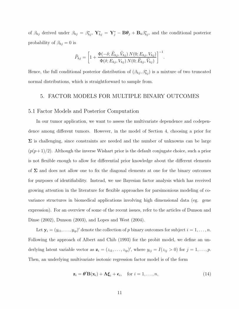
Let yi = (yi1, . . . , yip)′ denote the collection of p binary outcomes for subject i = 1, . . . , n.

Following the approach of Albert and Chib (1993) for the probit model, we define an un-

derlying latent variable vector as zi = (zi1, . . . , zip)′, where yij = I(zij > 0) for j = 1, . . . , p.

Then, an underlying multivariate isotonic regression factor model is of the form

zi = θ′B(xi) + Λξi + εi, for i = 1, . . . , n, (14)

11

where xi = (xi1, . . . , xiq)′ denotes a predictor vector for subject i, B(xi) = [1,B1(xi), . . . ,Bk(xi)]

′

denotes the basis function vector for the ith subject, in which Bh(xi) = (Bh(xi1), . . . , Bh(xiq))

and Bh(x) is defined in Section 2, θ = (θ1, . . . , θp) denotes the regression coefficient matrix,

in which θj = (β0j ,β′

1j , . . . ,β′

kj)′, βhj = (βhj1, . . . , βhjq)

′, βlhj is defined in Section 3, Λ is

a p× r factor loadings matrix, ξi = (ξi1, . . . , ξir)′ are independent standard normal factors,

and εi ∼ N(0,Σ), with diagonal covariance matrix Σ = diag(1, . . . , 1, σ2p1+1, . . . , σ

2p). The

resulting marginal density integrating out ξi is zi ∼ N(θ′B(xi),ΛΛ′ + Σ).

Let Y denote the n × p matrix of outcomes, i.e. Y = (y1, . . . ,yn)′. The corresponding

underlying latent variable matrix is Z = (z1, . . . , zn)′. Then we can write model (14) as

Z = Bθ + ΞΛ′ + ε, (15)

where B = (B(x1), . . . ,B(xn))′ is the n × (kq + 1) basis function matrix, θ and Λ are the

coefficient matrix and the p× r factor loadings matrix defined above, respectively, Ξ is the

n× r factor matrix, and ε = (ε1, . . . , εn)′ is the n× p normal error matrix. Given a random

sample of observations Y and a prior density π(Ξ,Λ, θ,Σ) on the parameters of the model,

the joint posterior distribution of the parameters and the latent variables Z is

π(Z,Ξ,Λ, θ,Σ|Y) = (2π)−np

2 |Σ|−n2 exp

{−

1

2tr(ε′εΣ−1)

}

×n∏

i=1

p1∏

j=1

{I(zij > 0)I(yij = 1) + I(zij ≤ 0)I(yij = 0)}

×π(Ξ,Λ, θ,Σ), (16)

where tr(A) is the trace of matrix A.

In order for the model to be identified, we need to place restrictions on the factor

loadings matrix Λ = (Λ1, . . . ,Λp)′. We follow the common convention of using a lower

triangular structure with λjk = 0 for all k > j, λkk > 0 for k = 1, . . . , r, and λjk ∈ < for

j > k. Assuming a priori independence, we then choose π(λkk) ∝ N(E0,kk, V0,kk)I(λkk > 0)

for k = 1, . . . , r, and π(λjk) = N(E0,jk, V0,jk) for j = k + 1, . . . , p and k = 1, . . . , r. For

12

σ2j , j = p1 +1, . . . , p, we choose inverse gamma priors, π(σ2

j ) = IG(c1, d1). The priors for the

other parameters are chosen as in Section 3.2. The full conditional posterior distributions

for all parameters and latent variables can be derived from (16) (refer to the Appendix).

The MCMC algorithm of Section 4 can be modified by replacing step (2) with steps for

updating the underlying normal variables {zij}, latent factors {ξi}, and factor loadings from

their conjugate full conditional posterior distributions, while also modifying the conditional

distributions used in steps (1), (3) and (4) slightly. Samples from the joint posterior distri-

bution of the parameters and the latent variables are generated by repeating these steps for

a large number of iterations after apparent convergence.

It is of interest to assess how high body weight needs to be before there is an increase

in tumor incidence relative to low weight animals. For the jth tumor type, this body weight

corresponds to the first increase in fj(·), which corresponds to the weight bj = min{xi :

xi ∈ (γh−1, γh], βhj > 0}. The posterior densities of bj, for j = 1, . . . , p, can be estimated

directly from the MCMC output. Also, of substantial interest is the posterior probability

that the jth tumor type exhibits an overall increase in incidence across the range of body

weights observed in the data base. The null hypothesis of no increase in incidence for the

jth tumor can be expressed as: H0j : β1j = · · · = βkj = 0, and we can easily estimate

Pr(H0j | data) by averaging model indicators across MCMC iterates collected after burn-in.

However, it is not enough to assess whether there is an overall increasing trend, we want

to assess whether incidence increases only for very heavy animals in the upper range of the

distribution or there is an increase in risk even for average weight animals. This question has

design implications, since the very heavy animals can potentially be removed by selective

breeding (there has been a trend towards fatter animals provided by the animal breeders).

In addition, to the extent that such trends reflect human health, it is certainly interesting

whether very thin individuals are at lower risk than average weight animals. Such questions

can be addressed using our Bayesian approach by estimating posterior probabilities of an

13

increase within particular ranges of body weight, which is straightforward by again averaging

appropriately-defined model indicators.

5.2 Generalizations: Covariates and Multilevel Models

Let wi = (wi1, . . . , wiC)′ denote a C × 1 vector of additional covariates for subject i, which

are assumed to have linear effects. The model (15) can be extended as

Z = Bθ + ΞΛ′ + Wα + ε, (17)

where W = (w1, . . . ,wn)′ and α = (α1, . . . ,αp), with αj = (α1j , . . . , αCj)′. Assume that the

prior for αj is Np(0, c0Ip). The full conditional posterior distribution for αcj, c = 1, . . . , C,

j = 1, . . . , p is

π(αcj|Zj,Ξ,Λj, θj,W(−c),α(−c)jc0, σ2j ) ∝ N(C∗W′

c(Zj − Bθj − ΞΛ′

j − W(−c)α(−c)j), C∗),

where Wc denotes the cth column of W, W(−c) denotes W without the cth column, α(−c)j

denotes αj without the cth element, and C∗ = (c−10 + W′

cWcσ−2j )−1.

In the tumor application, we have data from multiple studies and it is necessary to

accommodate possible heterogeneity. For this reason, we generalize our model to include

study-specific random effects for the different outcome types. In particular, we include

the random effects ζi = (ζi1, . . . , ζip)′ (i = 1, . . . , n), where i now indexes the study (or

cluster), j indexes subjects within clusters (j = 1, . . . , ni), and ζiuind∼ N(0, σ2

2u) for outcomes

u = 1, . . . , p. The data are of the form (yij,xij) (i = 1, . . . , n; j = 1, . . . , ni) where ni denotes

the number of observations in cluster i. Then we can rewrite the multivariate isotonic

regression factor model (14) as follows

zij = θ′B(xij) + Λξij + ζi + εij. (18)

In cluster i, the model (18) can also be written as

zi = B(xi)θ + ΞiΛ + 1niζ ′

i + εi, (19)

14

where zi = (zi1, . . . , zini)′, Ξi is the ni × r factor matrix, and εi = (εi1, . . . , εini

)′ is the ni × p

normal error matrix. Assuming that the prior for σ−22u is G(κ1, κ2), we can obtain the full

conditional for σ−22u as follows

π(σ−22u |ζ) ∝ G

(κ1 +

n

2, κ2 +

1

2

n∑

i=1

ζ2iu

).

The full conditional for ζi is

π(ζi|zi, ξi,Λ, θ) ∝ N(Vζ

i

Σ−11 (zi − B(xi)θ − ΞiΛ)′1ni

, Vζi

),

where Vζi

= (Σ−12 +niΣ

−11 )−1, Σ1 and Σ2 are covariance matrices of εij and ζi, respectively.

These full conditional distributions are easily simulated.

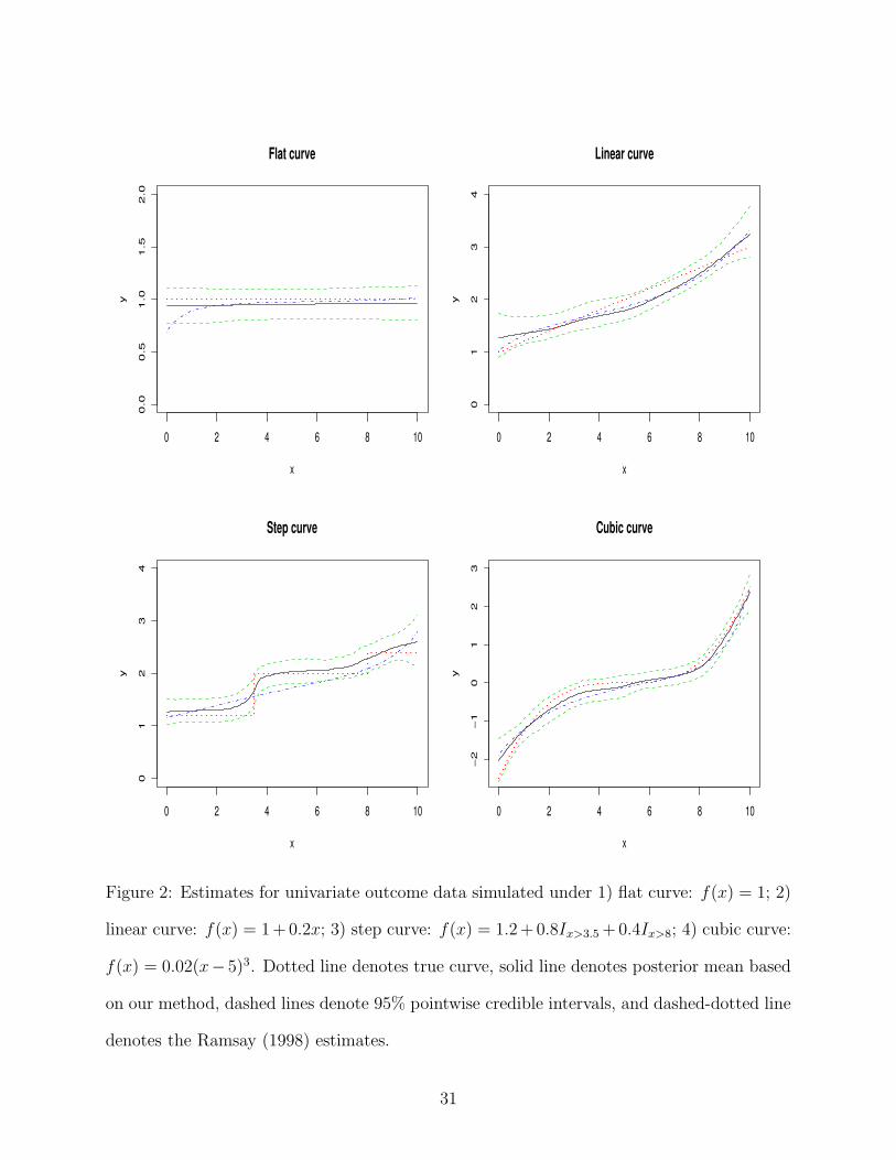
6. SIMULATION STUDY

We conducted a simulation study to evaluate the behavior of the proposed procedure. We

first compare the estimates of our proposed approach without the SUR component with

the Ramsay (1998) smooth monotone function estimator. We generated data from yi ∼

N(f(xi), 1) with f(x) chosen as 1) flat curve, 2) linear curve, 3) step curve, and 4) cubic curve,

with the predictor values generated from xi ∼ Uniform(0, 10), for i = 1, . . . , n = 200. We

chose priors for intercept β0 and the error variance as N(0, 10) and IG(0.1, 0.1), respectively.

The priors for τ and δ are chosen as G(2, 1) and G(1.25, 25), respectively. We also set grid

number k to be 100.

We ran our MCMC algorithm for 10,000 iterations after a 5,000 burn-in. The samples

passed convergence diagnostic tests in CODA (Best et al., 1995). We chose a set of MCMC

samples for inference by thining every 5 steps in the chain. We also conduct a sensitivity

analysis to the choice of prior by rerunning all of the analyses for different choices of the

hyperparameters, including (i) priors with variance ×2; (ii) priors with variance /2; and (iii)

priors with different means in a range consistent with our prior expectation.

15

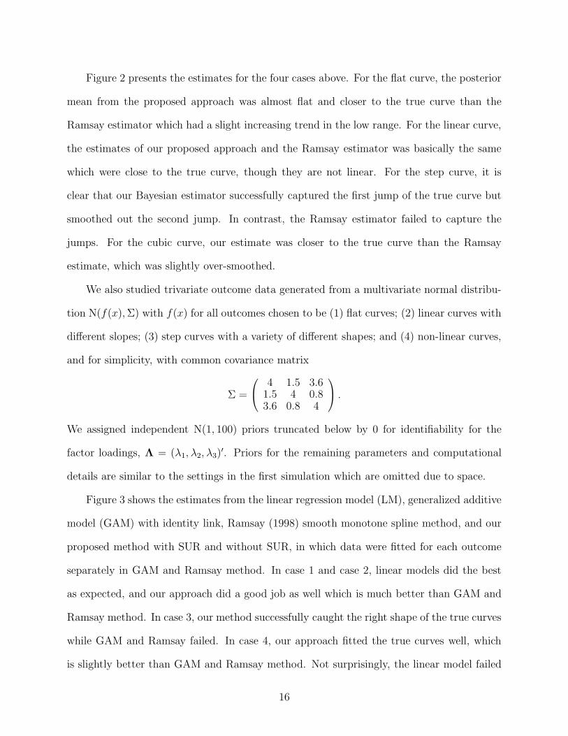
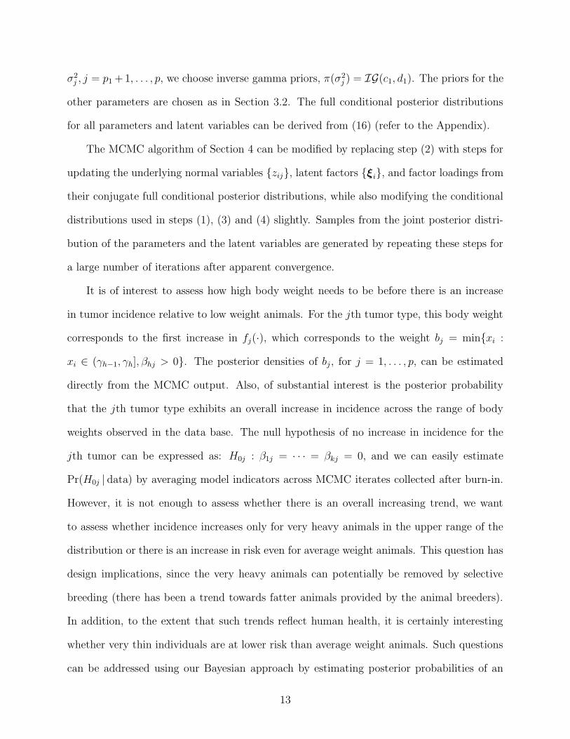
Figure 2 presents the estimates for the four cases above. For the flat curve, the posterior

mean from the proposed approach was almost flat and closer to the true curve than the

Ramsay estimator which had a slight increasing trend in the low range. For the linear curve,

the estimates of our proposed approach and the Ramsay estimator was basically the same

which were close to the true curve, though they are not linear. For the step curve, it is

clear that our Bayesian estimator successfully captured the first jump of the true curve but

smoothed out the second jump. In contrast, the Ramsay estimator failed to capture the

jumps. For the cubic curve, our estimate was closer to the true curve than the Ramsay

estimate, which was slightly over-smoothed.

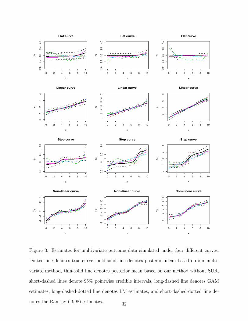
We also studied trivariate outcome data generated from a multivariate normal distribu-

tion N(f(x),Σ) with f(x) for all outcomes chosen to be (1) flat curves; (2) linear curves with

different slopes; (3) step curves with a variety of different shapes; and (4) non-linear curves,

and for simplicity, with common covariance matrix

Σ =

4 1.5 3.61.5 4 0.83.6 0.8 4

.

We assigned independent N(1, 100) priors truncated below by 0 for identifiability for the

factor loadings, Λ = (λ1, λ2, λ3)′. Priors for the remaining parameters and computational

details are similar to the settings in the first simulation which are omitted due to space.

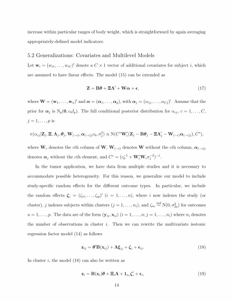
Figure 3 shows the estimates from the linear regression model (LM), generalized additive

model (GAM) with identity link, Ramsay (1998) smooth monotone spline method, and our

proposed method with SUR and without SUR, in which data were fitted for each outcome

separately in GAM and Ramsay method. In case 1 and case 2, linear models did the best

as expected, and our approach did a good job as well which is much better than GAM and

Ramsay method. In case 3, our method successfully caught the right shape of the true curves

while GAM and Ramsay failed. In case 4, our approach fitted the true curves well, which

is slightly better than GAM and Ramsay method. Not surprisingly, the linear model failed

16

in case 3 and 4. We also note that separate fit from our approach without SUR has less

accuracy due to the neglect of dependence among outcomes.

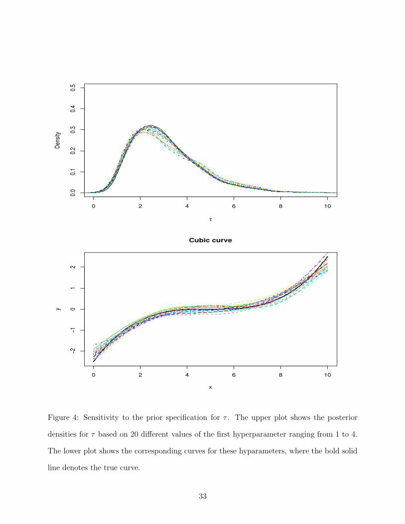
Figure 4 presents the posterior densities for τ based on 20 different values of the first

hyperparameter of (c, d) ranged from 1 to 4, and the corresponding curves to these hypa-

rameters. The plot shows the robustness of the curves to this prior specification.

7. MULTIPLE TUMOR SITE DATA APPLICATION

The data used in our application are from the National Toxicology Program (NTP) historical

control database for long-term rodent carcinogenicity bioassays. In this article we focus on

1209 male rats, with data consisting of individual animal body weights in grams at 12 months,

age at death, and 0/1 tumor indicators for 8 of the most frequently occuring tumor types.

The range of body weights for male rats is between 287.9 and 581.7 grams, with a median

of 479.7. We incorporate age at death as a covariate into the model (Dinse and Lagakos,

1983). The objective of the study is to model the 8 binary outcomes as a function of body

weight, allowing for correlation among the outcomes.

Our strong a priori belief is that tumor incidence is non-decreasing as 12 month body

weight increases, though certain tumor types may not depend on body weight and we are

uncertain how high body weight needs to be before there is an increase in incidence. We

analyze the data using our Bayesian approach in which a non-decreasing constraint is in-

corporated in the regression function for each outcome. We consider a two level Bayesian

multivariate isotonic regression model, with a single animal-specific factor, ξi, measuring

the susceptibility of animal i to tumor development and with study-specific random effects,

ζi = (ζi1, . . . , ζi8), for each tumor type. Since the outcomes are binary, the εi in (14) becomes

an independent normal random variate vector with mean zero and identity matrix Σ, i.e.

Σ =diag(1, . . . , 1).

To specify the degree of smoothing in the MRF prior, we chose π(τ) = G(2, 1) and

17

τ0 = 2, which corresponds to a moderate to high degree of smoothing. The factor loadings,

Λ = (λ1, . . . , λ8)′, are assigned independent N(1, 100) priors truncated below by 0 for iden-

tifiability. Variance of 100 corresponds to a highly diffuse specification for these parameters.

For the prior on the parameter δ, which controls the probabilities allocated to flat regions

of the regression functions, we chose G(1.5, 30). This prior is centered on E(δ) = 0.05 with

standard deviation 0.04. A value of 0.05 or less for the slope was considered to be effectively

0 in the context of the application (note that the body weights were standardized prior to

analysis). The prior for β0 is chosen as N(0, 10I) with 10 to correspond to a vague speci-

fication for the intercept. A diffuse prior for the survival effect coefficients, α, is chosen as

N(0, 10I). Finally, the prior for σ−22u is chosen as G(0.5, 50). We chose the potential knots

γ to correspond to an equally-spaced grid of k = 100 points spanning the range of body

weights observed in the data base.

We ran our MCMC algorithm for 50,000 iterations after a 10,000 burn-in. Diagnostic

tests showed rapid convergence and efficient mixing. A sample of size 2,000 was obtained by

thinning the MCMC chain by a factor of 25. To conduct a sensitivity analysis to the choice

of prior, we reran all of the analyses for different choices of the hyperparameters, including

(i) priors with variance ×2; (ii) priors with variance /2; and (iii) priors with different means

in a range consistent with our prior expectation. Although we do not report the results

in detail, inferences tended to be quite robust to the prior specification. Table 1 shows

the probabilities of getting the tumor for an animal with the mean body weight, where the

hyperparameters (c, d) for the prior of τ are fixed at (2, 1) while the hyperparameters (e, f)

for the prior of δ are chosen with different values. It appears that with the mean body

weight, an animal has a big chance to have leukaemia and kidney tumors.

To compare our Bayesian results with a simple frequentist regression analysis, we also

fit the data using an unconstrained probit GAM separately for each tumor type without

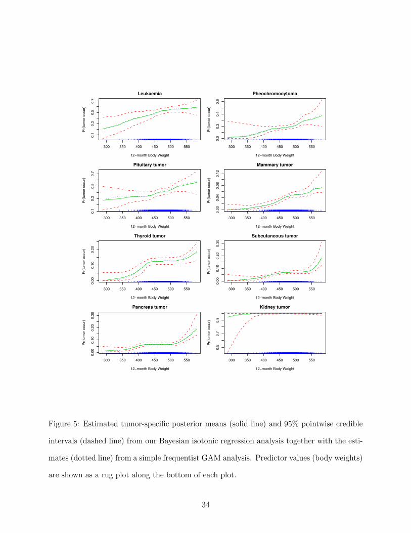
accounting for study-to-study heterogeneity. Figure 5 shows the comparison of the estimated

18

tumor type-specific incidence curves as a function of body weight for our Bayesian model

and the GAM model, together with the pointwise 95% credible intervals from our Bayesian

analysis. The estimated posterior mean of the tumor incidence curve for each tumor site

under our Bayesian approach is similar to that from the unconstrained frequentist GAM

analysis, which is reassuring in that it suggests that the order restriction and prior structure

is not introducing a high degree of systematic estimation bias. A primary difference (in

addition to facilitating inferences on increasing regions of the regression curves) is that the

Bayesian isotonic regression approach yields much more precise estimates compared with the

unconstrained GAM model. In particular, the 95% credible intervals are much narrower than

those from the GAM model, even accounting for study-to-study variability (which tends to

increase uncertainty and widen the intervals). This is not surprising, since large gains in

efficiency due to incorporation of a non-decreasing constraint are expected.

The survival-adjusted probability of getting a tumor of a particular type tends to increase

non-linearly across the range of body weights observed in the data base, with the shape of

the regression function varying somewhat for the different tumor types under consideration.

Our Bayesian estimates maintain a strict non-increasing shape, while the frequentist uncon-

strained estimates exhibit small downturns at intermediate levels of body weight for thyroid

tumor, subcutaneous tumor and pancreas tumor. These deviations are all small and are

likely to reflect estimation uncertainty instead of evidence against the order restriction. The

frequentist GAM analysis gives non-significant p-values for trend tests for all tumor types

while our Bayesian approach provides clear evidence of increasing response trends, with the

posterior probability of the null hypotheses being less than 0.03 for each tumor type. The

increasing trend in tumor incidence with increasing body weight for mammary tumor and

pituitary tumor is consistent with the results of Seilkop (1995) and Haseman et al. (1997).

We have also detected significant body weight-tumor incidence associations for additional

tumors not flagged in these earlier analyses. In particular, pheochromocytoma tumor, thy-

19

roid tumor and pancreas tumor, whose posterior probability of the null hypotheses is 0.015,

0.023 and 0.026, respectively, were not judged as body weight dependent by previous authors.

This is likely due to increased power of the incorporation of the non-decreasing constraint.

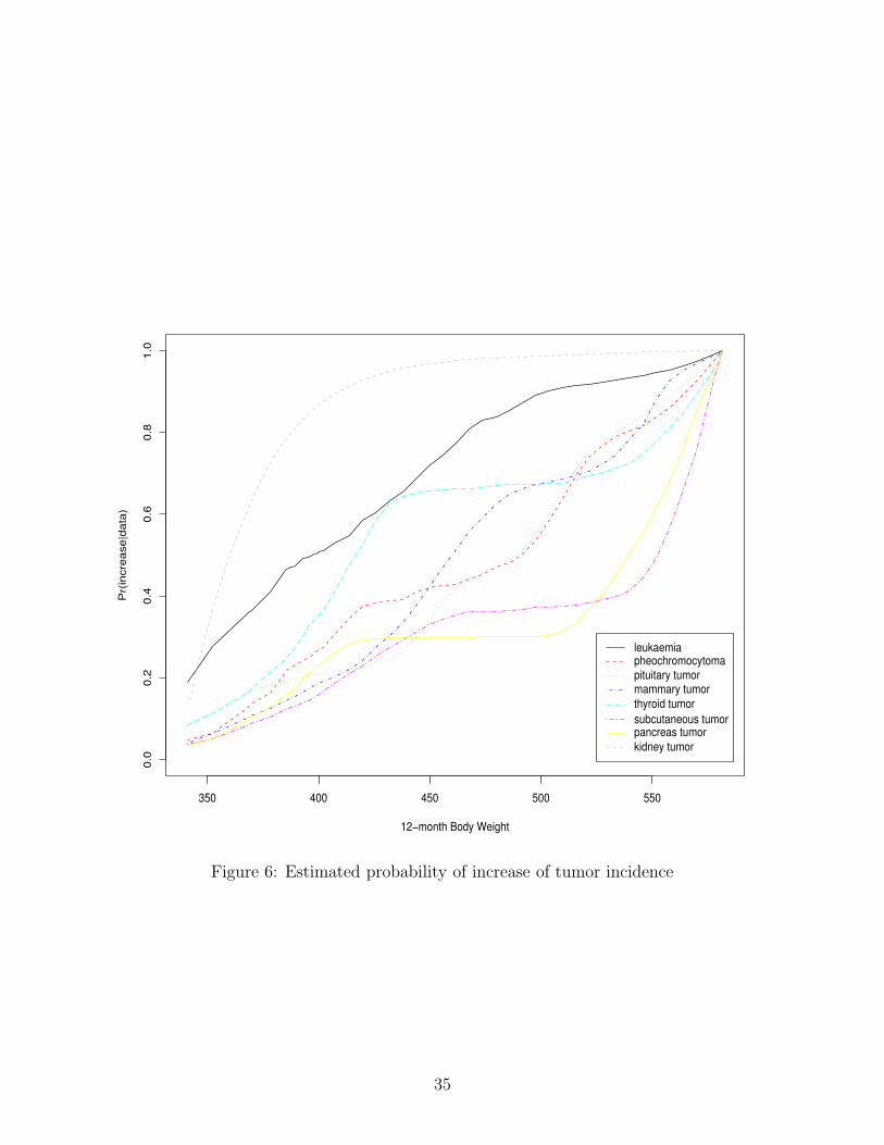
A clear advantage of our analysis is that we have a formal framework for assessing

evidence of trends, not only overall across the range of observed body weights but also

within particular regions. Figure 6 presents the estimated probability of an increase in

the tumor-specific incidence by each body weight relative to animals of low body weight.

Formally, these estimated curves are simply the posterior probabilities that fj(x) exhibits

at least one increase (i.e., is not flat) within the interval [γ0, x]. These probability curves

can be calculated easily from the MCMC output. Increases in body weight up to 425 grams

appear to increase kidney tumor incidence significantly, but the curve flattens out at higher

body weights at which essentially all the rats have tumors. The high incidence of kidney

tumors in male rats is a well known phenomenon, which leads to substantial mortality. For

thyroid and pancreas tumors, probabilities of an increase are quite stable at the range of

body weight between 430 and 500 grams, implying that these two tumors do not increase in

incidence when body weight increases within this range. In contrast, body weight appears

not to affect the increase of subcutaneous tumors at the body weight range of 470 and 525

grams. We can also obtain some detailed information in Figure 6. At the lower range of

body weight of being below 425 grams, the increase of leukaemia, thyroid tumor and kidney

tumor is more sensitive to body weight than that of the other tumors. In contrast, the

increase of subcutaneous tumor and pancreas tumor shows a stronger link to the higher

body-weight range over 525 grams than that of the others. These results are robust to the

prior specification.

To allow for heterogeneity among studies in the historical control database, we have

incorporated study-specific random effects for each tumor. It is interesting to assess the

level of heterogeneity among studies in the different tumor types, adjusting for differences

20

in animal survival and body weight. NTP investigators are worried about a trend towards

increased tumor incidence over time attributable to increases in body weight, and it is

not clear how much residual study-to-study variability remains after taking into account

differences in animal weight. This data set is based on studies conducted before NTP changed

to a new diet in an attempt to limit heterogeneity among studies. Based on examining

posterior distributions, most of the random effect variances are close to 0.10, which represents

a small to moderate degree of heterogeneity on the scale of the linear predictor (although

this is not a formal test).

In addition, by using our Bayesian approach, we can estimate the threshold body weight

corresponding to the lowest weight such that there is an increased incidence relative to

animals at the bottom of the weight range. Table 2 presents posterior summaries of the

threshold body weight for each tumor. These threshold body weights vary substantially

for the different tumor types, which is consistent with previous studies showing that the

body weight effect is strongly dependent on tumor type. Interestingly, leukaemia seems

to be particularly sensitive, with the estimated increase in incidence occurring starting at

a body weight of 321.75 grams, which is only in the 0.08th percentile of the distribution.

This is consistent with the estimates presented in Figure 1. Hence, for certain tumors of

major public health concern, it appears that even normal weight animals are of increased

risk relative to thin animals. A verification of the generalizability of this result to humans

through epidemiologic studies would be interesting. Kidney tumors also exhibit an increase

starting at low body weights, but it is less clear that this result would pertain to humans,

given that almost all male rats develop kidney tumors.

8. DISCUSSION

In this article we have proposed a Bayesian approach for multi-site tumor data from

carcinogenicity experiments. A multivariate smoothing spline model is specified, which ac-

21

commodates dependency in the multiple curves through a hierarchical Markov random field

prior for the basis coefficients, while also allowing for residual correlation through a multi-

level factor model. We have described a generalized multivariate isotonic regression factor

model for binary outcomes. By incorporating positive prior probability to flat regions in-

stead of using a strictly increasing function, we allow inferences on the occurrence and local

of regions across which there is no effect of a predictor. The resulting regression curve esti-

mator has a shrinkage-type structure, which may limit problems with over-estimation bias

observed for certain restricted estimators.

This approach was motivated by the NTP application to body weight and tumor inci-

dence described in Section 6. Some of the appealing features of our approach were illustrated

in this application. First, precision of estimates can be improved substantially through incor-

poration of non-decreasing constraints on the regression curves. Second, our approach allows

one to investigate the risk of an increase in incidence attributable to increasing body weight

by a given amount, which was not fully addressed by previous studies. Such inferences are

of primary interest in the tumor application, since it is important to assess whether or not

body weight has an effect not just for obese animals but also across the normal range of

body weights observed. Based on our results, it is clear that even normal weight animals can

have increased risk of certain tumors, most notably leukaemia but for other tumor types as

well. Potentially, the same type of methods can be applied to epidemiologic data collected

in studies verifying the occurrence of such effects in humans.

Although the methods presented in this article are focused heavily on the analysis and

interpretation of the data from rodent carcinogenicity experiments, they can be applied in a

wide variety of settings. It is also straightforward to extend our method to deal with mixed

categorical and continuous outcomes. In most epidemiologic and toxicologic studies involving

a potentially-adverse exposure, such as dose of a chemical, it is reasonable to assume a non-

decreasing regression curve after adjusting for important confounding factors, such as age.

22

In such settings, in which one collects multivariate mixed discrete and continuous outcome

data, it is straightforward to apply the approach described in this article to perform inference

on the unknown regression function.

APPENDIX

The full conditional posteriors for the parameters in Section 5.2:

• The full conditional posterior distribution for ξi is N(Vξi

Λ′Σ−1(zi − θ′B(xi)), Vξi

),

where Vξi

= (Ir + Λ′Σ−1Λ)−1.

• The full conditional for σ2j is IG(c1 + n

2, d1 + 1

2(Zj − Bθj − ΞΛ′

j)′(Zj − Bθj − ΞΛ′

j)),

for j = p1 + 1, . . . , p, where Zj denotes the jth column of Z and θj denotes the jth

column of θ.

• The full conditional for λkk is N(Vkk(V−10,kkE0,kk + σ−2

k Ξ′

k(Zk − Bθk)), Vkk)I(λkk > 0),

for k = 1, . . . , r, where Vkk = (V −10,kk + σ−2

k Ξ′

kΞk)−1 and Ξk denotes the kth column

of Ξ. The full conditional distribution for λjk, j = k + 1, . . . , p, is N(Vjk(V−10,jkE0,jk +

σ−2j Ξ′

k(Zj − Bθj)), Vjk), where Vjk = (V −10,jk + σ−2

j Ξ′

kΞk)−1.

• The full conditional for τ is:

G(τ |c1 + (s− 1)pq, d1 +

∑s−1t=1 tr[C′C]

)π(β∗

1)π(β∗

k|β∗

k−1) k = 2s

G(τ |c1 + spq, d1 +

∑st=1 tr[C′C]

)π(β∗

1) k = 2s+ 1

where C = (β∗

2t −12(β∗

2t−1 + β∗

2t+1)).

• The full conditional for β0j is N(S1n(Zj − B(−1)θj(−1) − ΞΛ′

j), S), where S = (s−1 +

nσ−2j )−1, B(−1) denotes the basis function matrix without the first column and θj(−1)

denotes the θj without the first element.

• The full conditional for (βhjl, β∗

hjl) is I(βhjl = 0)PhjlN(−∞,δ)(β∗

hjl|Ehjl, Vhjl) + I(βhjl =

β∗

hjl)(1 − Phjl)N[δ,∞)(β∗

hjl|Ehjl, Vhjl), where (1) Ehjl and Vhjl are the conditional prior

23

mean and variance of β∗

hjl derived conditional on βhjl = 0; (2) Ehj = Vhjl(V−1hjlEhjl +

σ−2j B′

mZ∗

j(−m)) and Vhjl = (V −1hjl + σ−2

j B′

mBm)−1 are the unconstrained conditional

posterior mean and variance of βhjl derived under βhjl = β∗

hjl, in which Bm is the

mth column vector of B, m = (h− 1)q + l, B−m is the submatrix of B excluding the

mth column, θj(−m) is the subvector of θj excluding the mth element, and Z∗

j(−m) =

Zj − B−mθj(−m) − ΞΛ′

j; (3) Phj is the conditional posterior probability of βhjl = 0.

• The full conditional for underlying latent variable zij, for j = 1, . . . , p1, is N(B(xi)θj +

Λjξi, 1)[I(zij > 0)I(yij = 1) + I(zij ≤ 0)I(yij = 0)].

REFERENCES

Albert, J.H., and Chib, S. (1993), “Bayesian Analysis of Binary and Polychotomous Re-

sponse Data,” Journal of the American Statistical Association, 88, 669-679.

Bartolucci, F. and Besag, J. (2002), “A Recursive Algorithm for Markov Random Fields,”

Biometrika, 89, 724-730.

Best, N.G., Cowles, M.K. and Vines, S.K. (1995), CODA manual version 0.30. MRC

Biostatistics Unit, Cambridge, UK.

Brown, P.J., Vannucci, M., and Fearn, T. (1998), “Multivariate Bayesian Variable Selection

and Prediction,” Journal of the Royal Statistical Society, Series B, 60, 627-641.

Brumback, B.A., and Rice, J.A. (1998), “Smoothing Spline Models for the Analysis of

Nested and Crossed Samples of Curves,” Journal of the American Statistical Associa-

tion, 93, 961-976.

Chib, S. and Greenberg, E. (1998), “Analysis of Multivariate Probit Models,” Biometrika,

85, 347-361.

24

Denison, D., Holmes, C., Mallick, B. and Smith, A.F.M. (2002), Bayesian Methods for

Nonlinear Classification and Regression. London: Wiley.

Dinse, G.E., and Lagakos, S.W. (1983), “Regression Analysis of Tumor Prevalence Data,”

Applied Statistics, 32, 236-248.

Dunson, D.B., and Dinse, G.E. (2002), “Bayesian Models for Multivariate Current Status

Data with Informative Censoring,” Biometrics, 58, 79-88.

Dunson, D.B. (2003), “Dynamic Latent Trait Models for Multidimensional Longitudinal

Data,” Journal of the American Statistical Association, 98, 555-563(9).

Haseman, J.K., Young, E., Eustis, S.L., and Hailey, J.R. (1997), “Body Weight-Tumor Inci-

dence Correlations in Long-Term Rodent Carcinogenicity Studies,” Toxicologic Pathol-

ogy, 25, 256-263.

Hastie, T.J. and Tibshirani, R.J. (1990), Generalized Additive Models. London: Chapman

& Hall.

Holmes, C.C., Denison, D.G.T, and Mallick, B.K. (2002), Accounting for Model Uncer-

tainty in Seemingly Unrelated Regressions,” Journal of Computational and Graphical

Statistics, 11, 533-551.

Holmes, C.C. and Heard, N.A. (2003), “Generalised Monotonic Regression using Random

Change Points,” Statistics in Medicine, 22, 623-638.

James, W., and Stein, C.M. (1961), “Estimation with Quadratic Loss,” Proceedings of the

4th Berkeley Symposium 1, 361-379.

Lavine, M. and Mockus, A. (1995), “A Nonparametric Bayes Method for Isotonic Regres-

sion,” Journal of Statistical Planning and Inference, 46, 235-248.

25

Lee, C.I.C. (1996), “On Estimation for Monotone Dose-Response Curves,” Journal of the

American Statistical Association, 91, 1110-1119.

Lopes, H.F. and West, M. (2004), “Bayesian Model Assessment in Factor Aanlysis,” Sta-

tistica Sinica, 14, 41-67.

Mammen, E. (1991), “Nonparametric Regression under Qualitative Smoothness Assump-

tions,” Annals of Statistics, 19, 741-759.

Neelon, B. and Dunson, D.B. (2004), “Bayesian Isotonic Regression and Trend Analysis,”

Biometrics, 60, 398-406.

Ng, V.M. (2002), “Robust Bayesian Inference for Seemingly Unrelated Regressions with

Elliptical Errors,” Journal of Multivariate Analysis, 83, 409-414.

Parise, H., Wand, M.P., Ruppert, D., and Ryan, L.M. (2001), “Incorporation of Historical

Controls Using Semiparametric Mixed Models,” Applied Statistics, 50, 31-42.

Ramsay, J.O. (1998), “Estimating Smooth Monotone Functions,” Journal of the Royal

Statistical Society, Series B, 60, 365-375.

Robertson, T., Wright, F. T. and Dykstra, R. L. (1988), Order Restricted Statistical Infer-

ence. Wiley, New York.

Schmid, C.H. and Brown, E.N. (1999), “A Probability Model for Saltatory Growth,” In

Saltation and Stasis in Human Growth and Development: Evidence, Methods and

Theory, ed. M. Lampl, London: Smith-Gordon, 121-131.

Seilkop, S. (1995), “The Effect of Body Weight on Tumor Incidence and Carcinogenicity

Testing in B6C3F1 Mice and F344 Rats,” Fundamental and Applied Toxicology, 24,

247-259.

26

Smith, M., and Kohn, R. (1996), “Nonparametric Regression using Bayesian Variable Se-

lection,” Journal of Econometrics, 75, 317-344.

Staniswalis, J.G., and Lee, J.J. (1998), “Nonparametric Regression Analysis of Longitudinal

Data,” Journal of the American Statistical Association, 93, 1403-1418.

Wu, H.L. and Zhang, J.T. (2002), “Local Polynomial Mixed-Effects Models for Longitudinal

Data,” Journal of the American Statistical Association, 97, 883-897.

Zellner, A. (1962), “An Efficient Method for Estimating Seemingly Unrelated Regressions

and Tests for Aggregate Bias,” Journal of the American Statistical Association, 57,

348-368.

27

300 350 400 450 500 550

0.0

0.2

0.4

0.6

0.8

Leukaemia

12−month Body Weight

Pr(

tum

or o

ccur

)

300 350 400 450 500 550

0.0

0.2

0.4

0.6

Pheochromocytoma

12−month Body Weight

Pr(

tum

or o

ccur

)300 350 400 450 500 550

0.0

0.2

0.4

0.6

0.8

Pituitary tumor

12−month Body Weight

Pr(

tum

or o

ccur

)

300 350 400 450 500 550

0.0

0.4

0.8

Mammary tumor

12−month Body Weight

Pr(

tum

or o

ccur

)

300 350 400 450 500 550

0.0

0.2

0.4

0.6

Thyroid tumor

12−month Body Weight

Pr(

tum

or o

ccur

)

300 350 400 450 500 550

0.0

0.2

0.4

0.6

0.8

Subcutaneous tumor

12−month Body Weight

Pr(

tum

or o

ccur

)

300 350 400 450 500 550

0.0

0.2

0.4

0.6

0.8

Pancreas tumor

12−month Body Weight

Pr(

tum

or o

ccur

)

300 350 400 450 500 550

0.4

0.6

0.8

1.0

Kidney tumor

12−month Body Weight

Pr(

tum

or o

ccur

)

Figure 1: Estimated probability of developing a tumor of each type according to 52 week

body weight. The solid line is the unconstrained frequentist estimate from a smoothing

spline GAM model, fitted in S-PLUS using gam(), and the dashed lines are 95% confidence

limits.

28

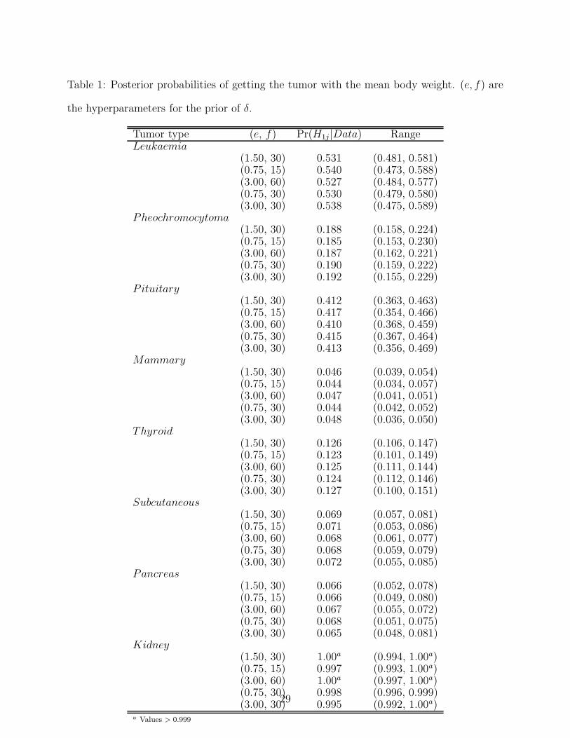
Table 1: Posterior probabilities of getting the tumor with the mean body weight. (e, f) are

the hyperparameters for the prior of δ.

Tumor type (e, f) Pr(H1j|Data) RangeLeukaemia

(1.50, 30) 0.531 (0.481, 0.581)(0.75, 15) 0.540 (0.473, 0.588)(3.00, 60) 0.527 (0.484, 0.577)(0.75, 30) 0.530 (0.479, 0.580)(3.00, 30) 0.538 (0.475, 0.589)

Pheochromocytoma(1.50, 30) 0.188 (0.158, 0.224)(0.75, 15) 0.185 (0.153, 0.230)(3.00, 60) 0.187 (0.162, 0.221)(0.75, 30) 0.190 (0.159, 0.222)(3.00, 30) 0.192 (0.155, 0.229)

Pituitary(1.50, 30) 0.412 (0.363, 0.463)(0.75, 15) 0.417 (0.354, 0.466)(3.00, 60) 0.410 (0.368, 0.459)(0.75, 30) 0.415 (0.367, 0.464)(3.00, 30) 0.413 (0.356, 0.469)

Mammary(1.50, 30) 0.046 (0.039, 0.054)(0.75, 15) 0.044 (0.034, 0.057)(3.00, 60) 0.047 (0.041, 0.051)(0.75, 30) 0.044 (0.042, 0.052)(3.00, 30) 0.048 (0.036, 0.050)

Thyroid(1.50, 30) 0.126 (0.106, 0.147)(0.75, 15) 0.123 (0.101, 0.149)(3.00, 60) 0.125 (0.111, 0.144)(0.75, 30) 0.124 (0.112, 0.146)(3.00, 30) 0.127 (0.100, 0.151)

Subcutaneous(1.50, 30) 0.069 (0.057, 0.081)(0.75, 15) 0.071 (0.053, 0.086)(3.00, 60) 0.068 (0.061, 0.077)(0.75, 30) 0.068 (0.059, 0.079)(3.00, 30) 0.072 (0.055, 0.085)

Pancreas(1.50, 30) 0.066 (0.052, 0.078)(0.75, 15) 0.066 (0.049, 0.080)(3.00, 60) 0.067 (0.055, 0.072)(0.75, 30) 0.068 (0.051, 0.075)(3.00, 30) 0.065 (0.048, 0.081)

Kidney(1.50, 30) 1.00a (0.994, 1.00a)(0.75, 15) 0.997 (0.993, 1.00a)(3.00, 60) 1.00a (0.997, 1.00a)(0.75, 30) 0.998 (0.996, 0.999)(3.00, 30) 0.995 (0.992, 1.00a)

a Values > 0.999

29

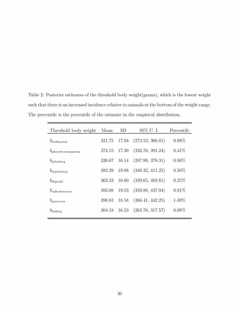
Table 2: Posterior estimates of the threshold body weight(grams), which is the lowest weight

such that there is an increased incidence relative to animals at the bottom of the weight range.

The percentile is the percentile of the estimate in the empirical distribution.

Threshold body weight Mean SD 95% C. I. Percentile

bleukaemia 321.75 17.94 (273.53, 366.81) 0.08%

bpheochromocytoma 374.15 17.30 (332.76, 391.24) 0.41%

bpituitary 326.67 16.14 (287.90, 378.31) 0.08%

bmammary 383.29 19.88 (340.32, 411.25) 0.50%

bthyroid 363.23 16.60 (339.65, 403.81) 0.25%

bsubcutaneous 392.08 19.53 (359.80, 437.94) 0.91%

bpancreas 398.83 18.58 (366.41, 442.25) 1.49%

bkidney 304.18 16.53 (263.78, 317.57) 0.08%

30

0 2 4 6 8 10

0.0

0.5

1.0

1.5

2.0

Flat curve

x

y

0 2 4 6 8 10

01

23

4

Linear curve

xy

0 2 4 6 8 10

01

23

4

Step curve

x

y

0 2 4 6 8 10

−2

−1

01

23

Cubic curve

x

y

Figure 2: Estimates for univariate outcome data simulated under 1) flat curve: f(x) = 1; 2)

linear curve: f(x) = 1+0.2x; 3) step curve: f(x) = 1.2+0.8Ix>3.5 +0.4Ix>8; 4) cubic curve:

f(x) = 0.02(x− 5)3. Dotted line denotes true curve, solid line denotes posterior mean based

on our method, dashed lines denote 95% pointwise credible intervals, and dashed-dotted line

denotes the Ramsay (1998) estimates.

31

0 2 4 6 8 10

2.0

2.5

3.0

3.5

4.0

Flat curve

x

y i1

0 2 4 6 8 10

2.0

2.5

3.0

3.5

4.0

Flat curve

x

y i2

0 2 4 6 8 10

2.0

2.5

3.0

3.5

4.0

Flat curve

x

y i3

0 2 4 6 8 10

01

23

4

Linear curve

x

y i1

0 2 4 6 8 10

12

34

56

7

Linear curve

x

y i2

0 2 4 6 8 10

24

68

Linear curve

x

y i3

0 2 4 6 8 10

0.0

1.0

2.0

3.0

Step curve

x

y i1

0 2 4 6 8 10

0.0

1.0

2.0

3.0

Step curve

x

y i2

0 2 4 6 8 10

01

23

4

Step curve

x

y i3

0 2 4 6 8 10

−2−1

01

23

Non−linear curve

x

y i1

0 2 4 6 8 10

−22

46

810

Non−linear curve

x

y i2

0 2 4 6 8 10

−40

24

68

Non−linear curve

x

y i3

Figure 3: Estimates for multivariate outcome data simulated under four different curves.

Dotted line denotes true curve, bold-solid line denotes posterior mean based on our multi-

variate method, thin-solid line denotes posterior mean based on our method without SUR,

short-dashed lines denote 95% pointwise credible intervals, long-dashed line denotes GAM

estimates, long-dashed-dotted line denotes LM estimates, and short-dashed-dotted line de-

notes the Ramsay (1998) estimates.32

0 2 4 6 8 10

0.0

0.1

0.2

0.3

0.4

0.5

τ

Dens

ity

0 2 4 6 8 10

−2−1

01

2

Cubic curve

x

y

Figure 4: Sensitivity to the prior specification for τ . The upper plot shows the posterior

densities for τ based on 20 different values of the first hyperparameter ranging from 1 to 4.

The lower plot shows the corresponding curves for these hyparameters, where the bold solid

line denotes the true curve.

33

300 350 400 450 500 550

0.1

0.3

0.5

0.7

Leukaemia

12−month Body Weight

Pr(

tum

or o

ccur

)

300 350 400 450 500 550

0.0

0.2

0.4

0.6

Pheochromocytoma

12−month Body Weight

Pr(

tum

or o

ccur

)

300 350 400 450 500 550

0.1

0.3

0.5

0.7

Pituitary tumor

12−month Body Weight

Pr(

tum

or o

ccur

)

300 350 400 450 500 5500.

000.

040.

080.

12

Mammary tumor

12−month Body Weight

Pr(

tum

or o

ccur

)

300 350 400 450 500 550

0.00

0.10

0.20

Thyroid tumor

12−month Body Weight

Pr(

tum

or o

ccur

)

300 350 400 450 500 550

0.00

0.10

0.20

0.30

Subcutaneous tumor

12−month Body Weight

Pr(

tum

or o

ccur

)

300 350 400 450 500 550

0.00

0.10

0.20

0.30

Pancreas tumor

12−month Body Weight

Pr(

tum

or o

ccur

)

300 350 400 450 500 550

0.5

0.7

0.9

Kidney tumor

12−month Body Weight

Pr(

tum

or o

ccur

)

Figure 5: Estimated tumor-specific posterior means (solid line) and 95% pointwise credible

intervals (dashed line) from our Bayesian isotonic regression analysis together with the esti-

mates (dotted line) from a simple frequentist GAM analysis. Predictor values (body weights)

are shown as a rug plot along the bottom of each plot.

34

350 400 450 500 550

0.0

0.2

0.4

0.6

0.8

1.0

12−month Body Weight

Pr(

incr

ea

se|d

ata

)

leukaemiapheochromocytomapituitary tumormammary tumorthyroid tumorsubcutaneous tumorpancreas tumorkidney tumor

Figure 6: Estimated probability of increase of tumor incidence

35