Embed Size (px)
Citation preview
University of Calgary
PRISM: University of Calgary's Digital Repository
Graduate Studies Legacy Theses
2001
Bearing condition monitoring and fault diagnosis
Chen, Ping
Chen, P. (2001). Bearing condition monitoring and fault diagnosis (Unpublished master's thesis).
University of Calgary, Calgary, AB. doi:10.11575/PRISM/23398
http://hdl.handle.net/1880/40657
master thesis
University of Calgary graduate students retain copyright ownership and moral rights for their
thesis. You may use this material in any way that is permitted by the Copyright Act or through
licensing that has been assigned to the document. For uses that are not allowable under
copyright legislation or licensing, you are required to seek permission.
Downloaded from PRISM: https://prism.ucalgary.ca

NOTE TO USERS
This reproduction is the best copy available.

THE UNIVERSITY OF CALGARY
Bearing Condition Monitoring and Fault Diagnosis
by
Ping Chen
A THESIS
SUBMITTED TO THE FACULTY OF GRADUATE STUDIES
IN PARTIAL FULFILLMENT OF THE REQUIREMENTS FOR THE
DEGREE OF MASTER OF SCIENCE
DEPARTMENT OF MECHANICAL AND MANUFACT'UMNG ENGINEERING
CALGARY, ALBERTA
DECEMBER, 2000
0 Ping Chen 2000

National Library BibliotMque nationale du Canada
Acquisitions and Acquisitions et Bibliographic Services services bibliiraphiques 395 woahgtm Street 395. rue WsOingeml OItawoON K l A W OlhwaON K l A W CMada Canada
The author has granted a non- exclusive licence allowing the National Li* of Canada to reproduce, loan, distn'bute or sell copies of this thesis in microform, paper or electronic formats.
The author retains ownership of the copyright in this thesis. Neither the thesis nor substantial extracts &om it may be printed or otherwise reproduced without the author's permission.
L'auteur a accord6 une licence non exclusive pennettant a la BibliothQue nationale du Canada de reprochire, pr&ter, distnbuer ou vendre des copies de cette these sous la forme de microfiche/^ de reproduction sur papier on sur format eIectronique .
L'auteur conserve la propnete du droit d'auteur qui proege cette these. Ni la these ni des extraits substantiels de celle-ci ne doivent &re imprim6s on autrement reproduits sans son autoxisation.
ABSTRACT
Bearing condition monitoring and fault diagnosis have been studied for many years.
Popular techniques include those through advanced signal processing and pattern
recognition technologies. Recently, some interesting results were published using pattern
recognition for bear& diagnosis by means of feahms extracted from vibration signals
through time domain and kquency domain analyses [Sun, et al, 19981. In this work,
segmentation parameters are proposed to f i d e r improve the sensitivity and reliability of
the technique. Parameters extracted from the segmentation analysis reflect the variation
of vibration signals associated with the bearing dynamics. A three-layered artificial
neural network is applied to accomplish the non-linear mapping fkom the feature space to
the two dimensional classification space. The mapping is conducted to create the best
cluster effect for training samples belonging to the same class. Successll non-linear
mapping through the neural network eliminates intra-class transformations as used in
[Sun, et al, 19981. Numerical experiments are performed to illustrate the effectiveness of
the method.
I am deeply indebted to Dr. Q. Sun, my supervisor, who has been a strong source of
inspiration throughout my project work. I have benefited greatly &om her invaluable
guidance and motivation. Her guidance has been very supportive in helping me complete
this project.
1 would also like to give a special thanks to the National Research Council of
Canada for its tinancia1 support and the Association of American Railroad for providing
the bearing testing &a
TABLE OF CONTENTS
. . .......................................................................................................... APPROVAL PAGE u
... mSTRA CT ...................................................................................................................... u1
ACKNOWLEDGEMENTS .Om.mO.mOm..O.....mO. ~ ~ ~ ~ m o ~ ~ w w ~ m ~ H ~ ~ ~ ~ ~ m ~ ~ ~ o ~ ~ m ~ e m ~ m ....mm...~w..~.....m~~wm~.m.~m~m~...m iv
TABLE OF CONTENTS ................................................................................................. v
. . LIST OF TABLES .......................................................................................................... vu ... LIST OF FIGURES ....................................................................................................... vrrr
CHAPTER ONE : INTRODUCTIONoooooooooooeoooooooooooooooooooooooooooooooooo.ooooo.o~oo 1
........................................................ 1 . 1 Machine Condition Monitoring and Diagnosis 1 1.2 Bearing Failure Modes ............................................................................................ 2
1.2.1 Fatigue ............................................................................................................ 2 1.2.2 Wear ................................................................................................................. 3 1.2.3 Corrosion .......................................................................................................... 4
......................................................................................................... 1 .2.4 Brinelling 4 ..................................................................................... 1.2.5 Lubrication Starvation 4
1.3 Dynamic Response due to Localized Fatigue Spalls ................................................ 5 .................................................................................................... 1.4 Vibration Analysis 6
.......................................................................................... 1 . 5 Vibration Measurement 8 1.6 Review of Vibration Analysis Techniques .............................................................. 9
1.6.1 Time Domain Techniques ............................................................................. 10 1.6.2 Frequency Domain Techniques ...................................................................... 1 1 1.6.3 Time-Frequency Analysis ............................................................................ IS
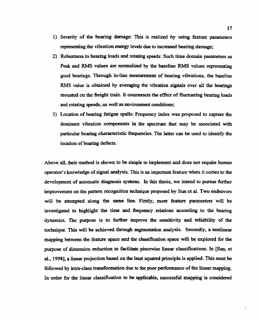
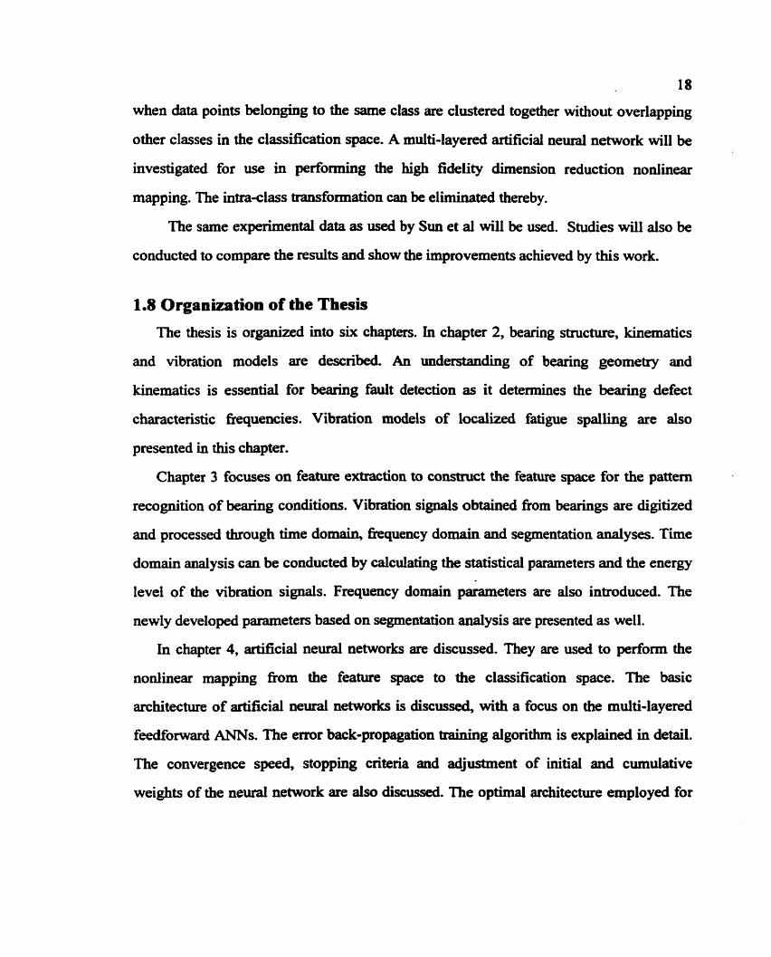
........................................................................................... 1.7 Objective of the Thesis 16 ...................................................................................... 1.8 Organization of the Thesis 18
CHAPTER TWO: BEARING KINEMATICS ................................. ....... 26
.................................................................................................... 2.1 Bearing Structure 26 ................................................................................................ 2.2 Bearing Kinematics 28 2.3 Vibration Models of Localized Fatigue S-g ................................................... 33
CHAPTER THREE: FEATURE EXTRACTION FOR PATTERN RECOGNITION ......................................................................................... 40
3.1 Feature Extraction .................................................................................................. 4 0 3.2 Time Domain Parameters ........................... .. ........................................................ 40
....................................................................... 3.2.1 Probability Density Function 4 1 ................................................................ 3.2.2 Root Mean Square and Peak Value 43
3.2.3 Statistical Parameters .................................................................................... 4 4 .............................................................................. 3.3 Frequency Domain Parameters 4 8 .............. ............................................ 3.4 Segmentation Analysis and Parameters ... 50
..................... ..................................................... 3.4.1 Segmentation Analysis ........ 50 3.4.2 Feature Extraction Using Segmentation Parameters ...................................... 54
CHAPTER FOUR: NEURAL NETWORKS FOR NONLINEAR MAPPING ................................................................................................... 69
............................................................................................................ 4.1 Introduction 69 ..................................................................................... 4.2 Artificial Neural Networks 70
4.2.1 Multilayer Feedforward Artificial Neural Networks ..................................... 73 ................................................. 4.2.2 Error Back-Propagation Training Algorithm 75
................................................................... .......................... 4.2.3 Convergence ... 81 ............................................................................................ 4.2.4 Stopping Criteria 83
4.2.5 Initial Weights and Cumulative Weight Adjustment ..................................... 84 ..................................... 4.3 Experimental Determination of Optimal Neural Network 85
4.3.1. Network Architectures with Optimal Hidden Layer ................................... 85 ..................... 4.3.2. Accelerated Convergence through Le-g-Rate Adaptation 86
.......................... CHAPTER FIVE : BEARING DEFECT DIAGNOSIS 96
.............................................................................................. 5.1 Experimental Studies 96 .................................................................................................... 5.2 Feature Selection 97 ................................................................. 5.3 Result of the Artificial Neural Network 99 ........................................................................................................ 5.4 Classification 101
................................................................................... .................. 5.5 Diagnosis ...... 102
CHAPTER SIX: CONCLUSION AND FUTURE WORK ......m..........m 1 1'8
.............................................................................. 6.1 S u w of Results Obtained 118 .................... 6.2 Limitations of the Present Method and Directions for Future Work 121
LIST OF TABLES
......................................................... Table 2.1 Bearing defect characteristic fkquencies 39
Table 3.1 a. Comparison of time domain pararneters for good bearing and defective
bearing ....................................................................................................................... 63
............................ Table 3.lb. Time domain parameters for bearings at different speeds 63
............................................ Table 32a. Frequency index for bearing in good condition 64
................................................ . Table 3.2b Frequency index for bearing with cup spalls 64
Table 33a . Time domain parameters of six segments for bearing with inner race defect
.................................................................................................................................... 65
Table 33b . Segmentation parameters (shaft fkquency) for bearing with inner race defect
................................................................................................................................. 65
Table 3.4a. Time domain parameters of six segments for bearing in good condition ..... 66
Table 3.4b. Segmentation parameters (shaft fkquency) for bearing in good condition .. 66
Table 35a . Time domain parameters of six segments for bearing with roller defect ...... 67
Table 3.5b. Segmentation parameters (cage fkquency) for bearing with roller defect ... 67
Table 3.6a. Time domain parameters of six segments for bearing with outer race defect
Table 3.6b. Segmentation parameters for bearing with outer race defect ........................ 68
Table 4.1 Performance comparison of hidden layer with different size .......................... 95
Table 5.1 Bearing conditions represented with class numbers ........................................ 96
..................................................................... Table 5 2 Bearing component dimensions 1 12
Table 5.3. Calculated 19 parameters for 1 15 samples .................................................... 1 13
Table 5.4 Normalized training sets ................................................................................ 1 14
Table 5.5. Network outputs compared with target outputs ............................................ 1 15
Table 5.6. Calculated parameters of 3 1 test data. ........................................................... 1 16
.......................................................... Table 5.7. Normalized parameters of 3 1 test data 1 17 vii
LIST OF FIGURES
Figure 1.1. Vibration signal h m a bearing with inner race defects ............................... 20
Figure 1.2. Comparison of two si@s with the same Peak values ................................. 21
Figure 1 3 . Power spectrum of a b e a ~ g with cone spalls .............................................. 22
Figure 1.4 Spectrum comparison .................................................................................... 22
.............................................................. Figure 1.5a . An impulse/time spectrum display 23
............................................................ Figure 1.5b. An envelope/tirne spectrum display 23
...................................................................... Figure 1.6. Short Time Fourier Transform 24
Figure 1.7. Wavelet Transform computed h m bearing vibration signals ...................... 25
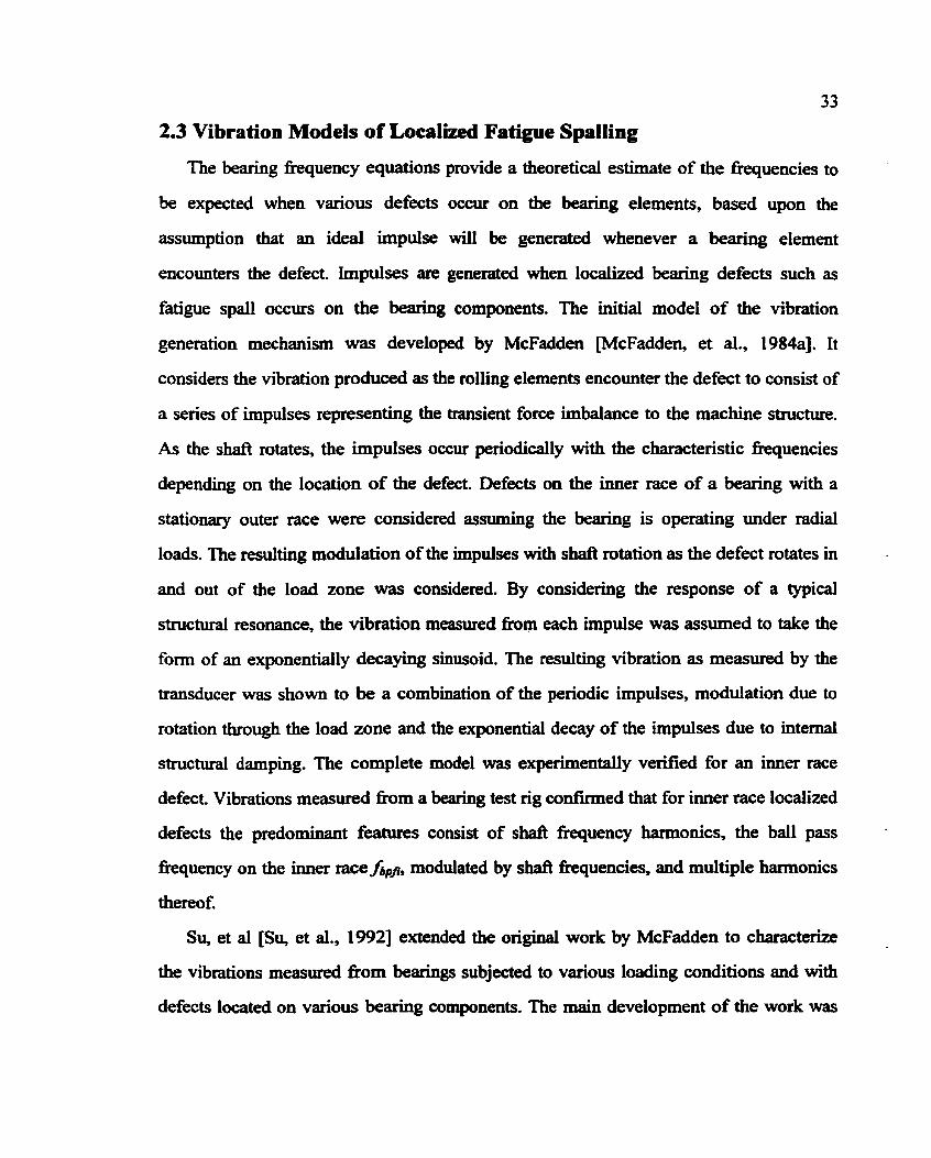
.......................................................................... Figure 2.1 Angular-contact ball bearing 36
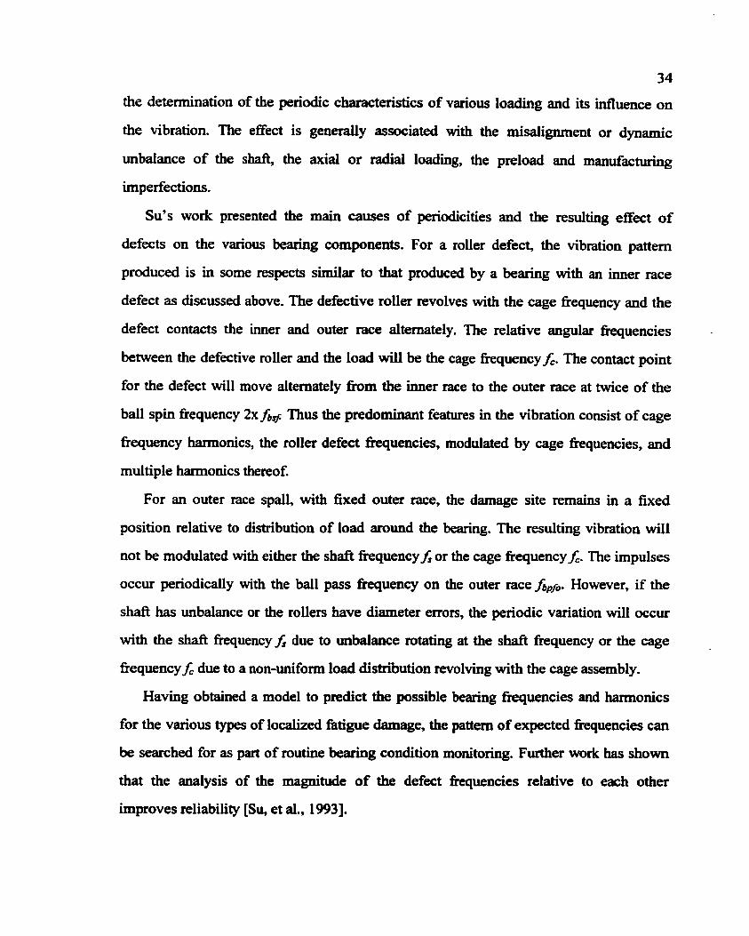
Figure 2 3 Tapered roller bearing ................................................................................... 36
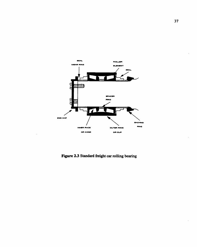
................................................................ Figure 2.3 Standard fieight car rolling bearing 37
................................. Figure 2.4 Schematic of a rolling element angular contact bearing 38
......................................................................... Figure 3.1.. b . Bearing vibration signals 56
........................................................................... Figure 3.2. Probability density function 57
.............................................. Figure 33a. b . Frequency spectra of the vibration signals 58
Figure 3.4.. Vibration signal for inner race defect in one second ................................... 59
Figure 3.4b . Vibration signal for inner race defect in one shaft revolution ..................... 59
....................................................................................... Figure 3.5 : Bearing under Load 60
......................................... Figure 3.6 a. Vibration signal from bearing with roller defect 61
Figure 3.6b. Signal from bearing with roller defect over one cage revolution ................ 61
............................... Figure 3.7 a. Vibration signal for outer race defect over one second 62
................. Figure 3.7b. Vibration signal for outer race defect over one cage revolution 62
Figure 4.1 Architecture graph of a multiplayer neural network with two hidden layers . 90
.............................................................................................. Figure 4.2 A neuron model 90
............................................................................ Figure 4.3 Sigmoid activation function 91 vi i i
Figure 4.4 Illustration of the ~ o n s of two passes: ..................................... ;.. ............ 91
.................................................................... Figure 4.5 A three-layered neural network 92
.................................................... Figure 4.6 Scheme 1 : incremental updating flowchart 93
.............................................................. Figure 4.7 Scheme 2: batch updating flewchart 94
.......................................... Figure 4.8 The neural network used for nonolinear mapping 95
........................................................................................ Figure 5.1 Multiple cup s p d s 104
Figure 5.2 Multiple cone spalls ...................................................................................... 104
................................................................................................. Figure 5 3 Broken roller 105
....................................................................... Figure 5.4 Roller bearing test rig at TTC 105
............................................................... Figure 5.5. Roller bearing mounted in test rig 106
........ Figure 5.6. Frequency spectrum versus bearing defect characteristic frequencies 106
Figure 5.7 a. An time/fkquency display of the signal in one revolution ....................... 107
........................................................... Figure 5.7b. Frequency spectra of each segment 108
Figure 5.8 Result of nonlinear mapping using neural networks .................................... 109
.............................................. Figure 5.9 Cluster centers evenly spaced on a unit circle 110
..................................................... Figure 5.10 Cluster centers arrayed on a unit square 110
............................................................ Fi y re 5.1 1 Classification and diagnosis results 1 1 1
CHAPTER ONE
INTRODUCTION
1.1 Machine Condition Monitoring and Diagnosis
Nowadays, manufacturing companies are making great efforts to reduce costs and
improve quality in order to maintain their competitiveness in the global marketplace. It is
recognized that significant cost savings and profitability can be achieved by higher
equipment availability, reliability, and maintainability. In order to accomplish this goal, it
is necessary to implement an effective machinery maintenance program wuang, et al,
1 9961.
The most important and expensive task in terms of labor time and cost in machinery
maintenance is fault detection and diagnostics. Without accurate identification of
m a k e faults, maintenance and production scheduling c a ~ o t be effectively planned;
the necessary repair work cannot be optimally scheduled. In addition, accurate fault
detection and diagnosis is essential for reducing troubleshooting and repair time. As a
result of correct and fast fault diagnosis, machine availability may be improved
significantly.
Bearings are essential components of most rotating machinery. The majority of the
problems in rotating machines are caused by faulty bearings pi, et al., 19891. Over the
last 30 years k ight cars have been equipped with tapered roller bearings. The railroad
industry suffers damages to equipment, wayside structures, and lading every year due to
derailments caused gy catastrophic wheel-bearing failure. Several wayside inspection
techniques are employed by railroads to identify defective bearings prior to failure.
Improving the reliability of bearing fault detection and diagnostics will reduce the
potential for derailment due to catastrophic bearing failure and enhance railroad safety.
2
The American Federal W o a d Administration (FRA) has focused its research
efforts on improving railroad safety. The current research is motivated by the interest of
the FRAY Transport Canada and the National Research Council of Canada on the
development of a technique to achieve the following objectives:
1. Reliably detect spalled race defects.
2. Reliably detect broken roller defects.
3. Reliably determine and indicate defect severity.
4. Significantly reduce system component maintenance requirements.
The bearing inspection systems currently used in railroad industry often fail to detect
overheated roller bearings. Other techniques based on processing the vibration signals
generated h m bearings, including time domain analysis, frequency domain analysis and
time-frequency analysis have also been studied for bearing fault detection and diagnosis.
However, none of the existing techniques can achieve the above objectives consistently,
which prompts the need for fkther investigation and development of the wayside bearing
defect diagnosis system.
1.2 Bearing Failure Modes
The normal service life of a rolling element bearing rotating under load is
determined by material fatigue and wear at the running surfaces. Premature bearing
failures can be caused by a large number of factors, the most common of which are
fatigue, wear, corrosion, brineiling and poor lubrication woward, 19941. The following
sections discuss the common modes of bearing failure.
1.2.1 Fatigue
A bearing subject to alternating normal loads could fail due to material fatigue after
a certain operation time. Fatigue damage begins with the formation of minute cracks
3
below the bearing surface. As loading continues, the cracks progress to the surface where
they cause material to break loose in the contact areas. The actual failure can manifest
itself as pitting, spalling or flaking of the bearing races or rolling elements. If the bearing
continues in service, the damage will spread in the vicinity of the defect due to stress
concentration. The surface damage severely disturbs the nominal motion of the rolling
elements by introducing short time impacts repeated at the characteristic rolling element
defect frequencies. As the damage continues to spread the repetitive nature of the impacts
will diminish as the motion of the rolling element becomes so irregular and disturbed that
it is impossible to distinguish between individual impacts. If the bearing were to continue
in service, the damage may spread to other raceways or rolling elements and eventually
lead to increased fiiction and temperature followed by complete seizure.
1.2.2 Wear
Wear is another common cause of bearing fdure. It is caused mainly by dirt and
foreign particles entering the bearing through inadequate sealing or due to contaminated
lubricant. The abrasive foreign particles roughen the contacting surfaces giving a dull
appearance. Severe wear changes the raceway profile, alters the roiling element profile
and diameter, and increases the bearing clearance. The rolling friction increases
considerably and can lead to high level of slip and skidding. The end result of this is
complete breakdown. Increasing wear will gradually introduce geometric errors in the
bearing. Non-uniform diameters of worn rolling elements will cause cage fkequency
vibration and harmonics to be produced m e , 19891 as the sequence of balls rotating
through the load zone is periodic with the cage rotation frequency. Geometric errors of
the raceways will resuit in the production of multiple harmonics of shaft speed being
produced.
4
1.2.3 Corrosion
Corrosion damage occurs when water, acids or other con taminants in the oil enter the
bearing assembly. This can be caused by damaged seals, acidic lubricants or
condensation which occurs when bearings are suddenly cooled fiom a higher operating
temperature in very humid air. The result is rust on the running surfaces which produces
uneven and noisy operations as the rust particles interfa with the lubrication. The rust
particles also have an abrasive effect which generates wear. The rust pits also form the
initiation sites for subsequent flaking and spalling.
1.2.4 Brinelling
Brinelling, manifests itself as regularly spaced indentations distributed over the entire
raceway circumference, corresponding approximately in shape to the Hertzian contact
area. Three possible scenarios causing brinelling are (1) when a bearing is subjected to
static overloading which leads to plastic deformation of the raceways, (2) when a
stationary rolling bearing is subjected to vibration and shock loads and (3) when a
bearing forms a loop for the passage of electric current. In all cases, the result will be
repetitive indentations of the raceways. In some instances, a large number of indentations
may occur as the bearing may occasionally be tumed slightly. The bearing operation will
be noisy and uneven in the presence of briwlling with each indentation acting like a
small fatigue site producing sharp impacts with the passage of the rolling elements.
Continued operation will lead to the development of spalling at the indentation sites.
1.2.5 Lubrication Starvation
Inadequate lubrication, either in tenns of quantity or quality, is one of the common
causes of premature bearing failure as it leads to skidding, slippage and bearing seizure.
At the highly stressed region of Hertzian contact, when there is insufficient lubricant, the
5
contacting SUtfaces will weld together, only to be tom apart as the rolling element moves
on. The three critical points of bearing lubrication occur at the cage-roller interface, the
roller-race interface and the cage-race interface. Lubricant starvation or improper
lubricant selection can have severe consequences as high temperatures can anneal the
bearing elements and reduce hardness and fatigue life. Eventually, bearing elements will
experience excessive wear which could cause catastrophic failure.
1.3 Dynamic Response due to Localized Fatigue Spalls
Rolling element bearings often have a tendency to fail by fatigue rather than wear-out
due to the low wear rate and high roller-rate contact load [Braun, et al., 19791. Since the
primary mode of bearing failure is due to localized fatigue spalling of bearing elements
pi, 1989; McFadden, 19901, this work focuses on dealing with fatigue spalls.
An undamaged bearing under load is subjefted to complex forces and moments.
These include static forces such as shaft loads and preloads, dynamic forces due to
centrifugal loads, fluid pressure, traction and fiction. For a good bearing operating at a
constant shaft speed and load, al l forces are in quasi-equilibrium.
When a rolling element encountem a defect on the bearing surface, a rapid localized
change in the elastic deformation of the elements takes place, and a transient force
imbalance occurs. The transient forces will then result in rapid accelerations of the
bearing components. Complex motions can occur such as oscillatory contact and impacts
between the roller and raceway, roller and cage, and cage and raceway as well as
skidding or slipping of the roller and cage.
Construction of dynamic models describing the bearing motion caused by defects has
been attempted. Gupta developed models that incorporate localized changes to the motion
of the raceways and rolling elements [Gupta, 1975; 1979a; 1979b; 1979c; 19811.
However, experimental verification of the model was only performed with Limited
6
examples [Gupta, et al., 19851. Measuring the motion of bearing components, such as
cage angular velocity, roller linear and angular velocity, etc., is an extremely difficult
task and prone to errors due to the inaccessibility of the bearing components.
For most rotating machinery, detecting the presence of a damaged bearing is not
sufficient. It is more important to determine the extent of the damage and its effect upon
bearing Life. Inspection of bearings removed from service with the existing wayside
inspection techniques showed that, in some instances, the defects present in the bearings
were not condemnable under cumnt Association of American Railroads guidelines for
reconditioning roller bearings. Furthermore, it is a common belief in the railroad industry
that such "minor" defects could survive for the remaining Life of the adjacent wheels and
that the removal of bearings with such defects is considered to be economically
disadvantageous with little or no net safety improvement plorom, 19941.
Fatigue in rolling element bearings is caused by the application of repeated stresses
on a finite volume of material. Because bearing materials are not homogeneous or equally
resistant to failure at all points, it occurs at the weakest point of the material. Therefore, a
group of supposedly identical specimens will exhibit wide variations in failure times
when operated under the same conditions. However, improvement in bearing materials,
lubrication and manufacturing technology has led to a large increase in bearing life and
reliability.
1.4 Vibration Analysis
Currently, there are two kinds of bearing inspection systems being used in railroad
industry: the Hot Box Detector (HBD) and the Acoustic Based Detector (ABD). The
HBD system uses wayside rail-mounted infrared (IR) transducers to monitor bearing
temperature as the train passes by the detector. The system issues an alarm if the bearing
temperature exceeds a preset limit. Such a system was originally designed for monitoring
7
fiction bearings. However, over the last 30 years, freight cars have been equipped with
tapered roller bearings. When the catastrophic failure of roller bearings happens, bearing
temperature increases within short period of time followed by axle journal bum-off.
Consequently, the HE3D often misses overheated roller bearings [Choe, et al., 19971. This
has a detrimental effect on the safety and efficiency of railroad operations.
In the late 70's, Acoustic Based Detectors were commercialized and applied for
wayside bearing inspections. Since then, there has been an increasing interest and
demand for the development of efficient and reliable devices based on acoustic sensory
signals. Existing ABD techniques are shown to be too sensitive to bearing incipient
damages and therefore are often over-safe. It becomes evident that advanced signal
processing techniques are desirable.
Machine vibrations are due to cyclic excitations to the machine. The excitation loads
exist during normal machine operation or could be due to changes in the dynamic
properties of the machine, such as certain component failure. These excitation forces are
transmitted to adjacent components or adjoining structure, causing parts of the machine
to vibrate at different resonance kquencies. A change in the vibration signal not only
indicates a change in machine conditions, but also oflen points to the problem. When a
machine is operating properly, vibration is small and constant. Faulty components usually
cause significant changes in machine dynamics leading to much higher vibration energy
levels with different patterns. The amount of information contained in the measured
vibration signals is immense.
The use of vibration measurement as a diagnostic tool is well established in various
engineering disciplines Fiu, et al., 19921. This non-intrvsive technique can be easily
applied to monitoring machinery conditions without interfering with machine operation.
It may be used to gain information about subsystems which are otherwise inaccessible.
The ability of vibration based techniques to detect and diagnose a broad range of faults in
8
a wide array of machine elements is one reason that it is often chosen as a preferred
method. The technique is non-intrusive and cost-effective, which makes it more attractive
for condition monitoring wechefske, et al., 199 13.
Vibration monitoring of rolling element bearings has consistently produced good
results because of developments in signal processing techniques. Pattern recognition
techniques have been investigated [Batchelor, 1978; Sun, et al., 1997, 1998; Wang, et al.,
19981 and shown to have the ability to deal with various machine operating conditions. In
this thesis, we further pursue pattern recognition analysis with the objective of increasing
reliability and sensitivity of the method.
1.5 Vibration Measurement
The success of any monitoring program largely depends on the accuracy of the
measurement. Given that the instnunentation is properly calibrated, measurements are
accurate when the sensor mounting does not limit the kquency and dynamic ranges of
the sensor and when measurements are always collected at the same locations
[Alguindigue, et al., 1993).
The measurement of machine vibration can be made using a wide array of
transducers. Microphones measuring the acoustic response of the machine have been
shown to provide useful diagnostic information [Smith, et al., 1988; Jammu, et al., 19971.
They can be used for non-contact vibration measurement and are inexpensive. The
parabolic microphone in particular has been shown to be effective as a remote acoustic
monitor of rolling element bearings and has been used effectively on railcar bearing
detection and diagnosis [Smith, 1988; Smith, 19921. By locating the microphone
statically at a distance of approximately 20 feet Grom the train, the parabolic microphone
is capable of eliminating off axis sound and concentrating on the direct sound. The main
drawbacks with microphonic recording systems are that their frequency response is
9
limited to the audible range, and that they are relatively insensitive to very low kquency
signal components.
The piezo-electric accelerometer which measures the acceleration of vibrations is
probably the most popular measurement transducer for vibration analysis in use today.
They have light weight, good temperature resistance, and wide frequency response and
dynamic range Fiathew, 19891. The hquency response is limited by the natural
fiequency of the system, and operation is usually limited to about 20%-30% of the
natural hquency of the transducer. The acceleration signals obtained from these
transducers are sometimes integrated to produce velocity or even displacement for
different applications. These signals are then processed in diverse ways to highlight
various aspects of the signal which can then be used in the detection and diagnosis of the
machine condition.
Velocity transducers measure the velocity of the machine casing to which they are
attached. They are capable of measuring down to almost DC. They have not found wide
acceptance for bearing fault detection as the frequency range available with
accelerometers is wider. A number of laser velocity measurement systems are also
available where the surface velocity of the machine is measured by the laser using the
Doppler shifting principle [Smith, 19921. The data used in this work were collected using
microphones and accelerometers.
1.6 Review of Vibration Analysis Techniques
The vibration signal obtained from operating machines contains information relating
to machine condition as well as noise. Further processing of the signal is necessary to
elicit idormation particularly relevant to bearing faults. Many techniques have been
employed to process the vibration signals in bearing fault detection and diagnosis. Three
10
common techniques, time domain techniques, frequency domain techniques and time-
fkquency analysis will be briefly reviewed.
1.6.1 Time Domain Techniques
Time series of the signal, if understood properly, can yield enormous amounts of
information. Further analysis is usually carried out so that important characteristics not
readily observed can be highlighted. Several techniques used in machine monitoring are
explained in the following paragraphs.
The most straightforward technique is simply to v i d y inspect portions of the time
domain waveform. Figure 1.1 shows vibration signal waveform for one second duration
obtained from a bearing containing inner race defects. The signal is digitized with a
sampling rate of 27WIz. Repetitive impacts can be observed at the time period
corresponding to the time interval Tbpfi (revolution of ball passing inner race) when
rolling elements pass the race damage, as indicated in Figure 1 .I . It can also be observed
that these repetitive impulses are modulated with the inner race rotation and therefore
similar patterns are repeated in every revolution of the inner race, Ti. If we zoom in to
look at the signal in 0.1 second, we can see three impacts which are spaced at Tbpn in
every period of inner race revolution Ti. Each impact excites the resonance of the
structure which rapidly decay due to the system damping. It should be pointed out that
bearing vibration signals do not always present the impacts so clearly. The total vibration
signal produced by a large machine containing many components may be very
complicated when viewed in the time domain, making it unlikely that a spalling defect in
a bearing may be detected by a simple visual inspection of the vibration wavefonn
WcFadden, 19901. Impulses are often masked by vibrations &om other components and
background noise. More sophisticated time domain techniques are desirable such as
through trending certain characteristic parameters.
11
The vibration si@s generated from bearings mounted on the railway k igh t car are
normally non-deterministic and non-stationary. Commonly used time domain parameters
are determined through the probability density distribution. These are Peak (Pk), Root
Mean Square value (RMS), Crest factor (Cf), Kurtosis value (Kv), Clearance factor (CU),
and Impulse factor (If). Peak and RMS can directly reflect the energy level of the
vibration. Cf and Kv can be used to indicate the spikiness of the signal associated with
the defect-induced impulses.
Suppose we have signall and signal2 with the same Peak value. If signall has higher
energy but is less spiky and signal2 is spikier with lower energy level, then we should
observe that signall has greater RMS value and signal2 has larger Cf and Kv. Figure 1.2
shows the waveforms of signdl and signal2 and values of these parameters are shown in
the caption.
Crest factor (Cf), kurtosis value (Kv), Clearance factor (Clf) and Impulse factor (If)
are non-dimensional statistical parameters. They are very effective in indicating incipient
fatigue spalling. But sometime these parameters fail to indicate the defects due to the
development of the failure. For example, if the defect becomes severe, Cf and Kv will
reduce to normal values. Therefore they are not very reliable and cannot be used in
isolation. Moreover, they cannot be used to directiy indicate the location of the defect.
1.6.2 Frequency Domain Techniques
Discrete Fast Fourier analysis of the time waveform has become the most popular
method of deriving the frequency domain signal. The signature spectnun so obtained can
provide valuable information with regards to machine conditions Flathew, 19891.
Spectral analysis and spectrum comparison are commonly used frequency domain
techniques. Envelope analysis or demodulating the time waveform prior to performing
the fast Fourier transform is also gaining popularity.
12
Spectral analysis is a very common technique when analyzing the vibration signal in
the fiequency domain [EshIeman, 1980; Taylor, 1980; McFadden, et al., 1984a;
ALfredson, et al., 1985a; Bannister, 1985; Igarashi, 1985; McFadden, et al., 1985;
Mechefske, et al., 1992; Mechefske, 19931. Power spectrum can be used to identify the
location of the defect by relating the defect characteristic frequencies to the major
frequency components in the spectrum. For bearing fault detection and diagnosis, a
detailed knowledge of the bearing defact characteristic fiequencies is required, which will
be discussed in chapter 2. Figure 1.3 shows the power spectrum of a bearing with an
inner race defect. We can see a dominant peak at the kquency of about 102Hz, which is
very close to the roller passing inner race fiequency (99Hz). It indicates the defect is on
the inner race.
Automatic detection of impulses at bearing characteristic fkequencies is not a simple
task for it involves searching of the spectnun for specific fiequencies related to all
relevant components including harmonics and sidebands of any of the defect frequencies
[Shi, et al., 19881. Difficulties lie in the fact that the energy of the bearing vibration is
spread across a wide frequency band and can be easily buried by the noise. The result is
that various resonances of the bearing and the surrounding structure will be excited by the
defect-induced impact.
Spectrum comparison has also been investigated for the purpose of signature analysis
mdall, 1985; Semdge, 1991; Succi, 19911. A baseline spectrum is taken when the
bearing is in good condition. The difference between the baseline and subsequent signal
spectrum is used to highlight changes in mechanical condition. The comparison is used to
locate those fkquencies in which significant increases in magnitude have occurred.
Figure 1.4 shows how spectral comparisons are performed. The reference spectrum is
first established as baseline for the bearing in good condition. When a new signal has
been recorded, the fhquency spectra can be calculated and compared with the reference.
13
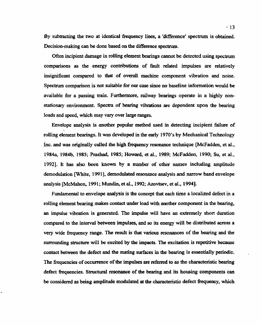
By subtracting the two at identical frequency lines, a 'difference' spectnun is obtained.
Decision-making can be done based on the difference spectrum.
Often incipient damage in rolling element bearings cannot be detected using spectrum
comparisons as the energy contributions of fault related impulses are relatively
insignificant compared to that of overall machine component vibration and noise.
Spectrum comparison is not suitable for our case since no baseline idomation would be
available for a passing train. Furthermore, railway bearings operate in a highly non-
stationary environment. Spectra of bearing vibrations are dependent upon the bearing
loads and speed, which may vary over large ranges.
Envelope d y s i s is another popular method used in detecting incipient failure of
rolling element bearings. It was developed in the early 1 970's by Mechanical Technology
Inc. and was originally called the high kquency resonance technique WcFadden, et al.,
1984% 1984b, 1985; Prashad, 1985; Howard, et al., 1989; McFadden, 1990; Su, et al.,
19921. It has also been known by a number of other names including amplitude
demodulation v t e , 199 11, demodulated resonance analysis and narrow band envelope
analysis WcMahon, 199 1 ; Mundin, et al., 1992; Azovtsev, et al., 19943.
Fundamental to envelope analysis is the concept that each time a localized defect in a
rolling element bearing makes contact under load with another component in the bearing,
an impulse vibration is generated. The impulse will have an extremely short duration
compared to the interval between impulses, and so its energy will be distributed across a
very wide frequency range. The result is that various resonances of the bearing and the
surrounding structure will be excited by the impacts. The excitation is repetitive because
contact between the defect and the mating surfaces in the bearing is essentially periodic.
The frequencies of occurrence of the impulses are referred to as the characteristic bearing
defect frequencies. Structural resonance of the bearing and its housing components can
be considered as being amplitude modulated at the characteristic defect frequency, which
14
makes it possible not only to detect the presence of the defect but also to identify the
location of the defect. Envelope analysis provides a mechanism for extracting the
periodic excitation or amplitude modulation of the resonance woward, 1 9941.
The envelope analysis involves passing the band-pass filtered signal through a half-
wave rectifier and then through a low-pass filter. The half-wave rectifier removes either
the positive or negative excursions of the signal to leave a succession of unipolar pulses,
still at the resonant frequency. Low-pass filtering removes the resonant fiequency and
smoothes these pulses. Figure 1.5a [SKF, 19931 shows the relationship between a time
domain repetitive impulse signal and its FFT spectrum conversion. It is clear from the
fiequency spectrum that there is a dominant impulse component at about the fiequency of
50Hz with exponentially decaying magnitude. Such impulses are also modulated by a
signal with lower fiequency (-Sk). However, when inspecting the frequency spectrum
in Figure 1.54 the 5OHz component was indicated by the peak but the S H z component
was buried in the sidebands. In the application of machine condition monitoring,
detection of both components is important, and detecting the lower fiequency component
may become more critical. This could be achieved through wrapping the signal by the
envelope as shown in Figure 1.5b and the subsequent spectrum shows dominant
components at the fkquency of SHz.
Successll application of envelope analysis requires knowledge and experience in
locating the existence of the camer frequencies before band pass filtering can proceed.
Kurtosis value has been suggested as an aid to identify a suitable carrier frequency
pamister, 19851, but it should also be recognized that the machine being monitored
might not even contain carrier fkquencies. Moreover, envelope analysis is not suitable
for detecting extensively damaged bearings. A more severely damaged bearing presents a
more random dynamic response to impacts and thus makes it difficult to identify the
carrier fiequency. It may be reasonable to consider extensively spread spalls as the sum
15
of smaller ones, each of which will produce an envelope spectrum. When many spectra
are summed together? some components may cancel each other while others may be
reinforced due to the difference in phases. Consequently, modulation sidebands may
dominate the envelope spectrum instead of the hdamental impact frequencies and their
harmonics.
1.6.3 Time-Frequency Analysis
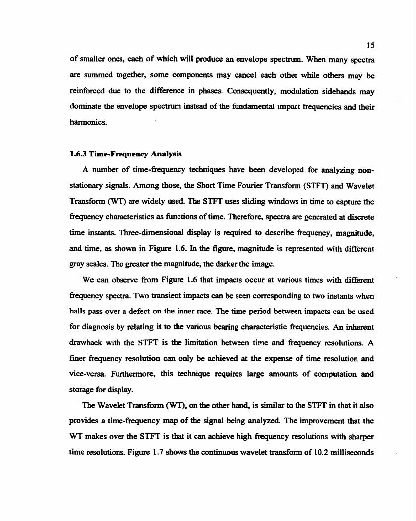
A number of time-frequency techniques have been developed for a n a l y ~ g non-
stationary signals. Among those, the Short Time Fourier Transform (STFT) and Wavelet
Transform (WT) are widely used. The STFT uses sliding windows in time to capture the
frequency characteristics as functions of time. Therefore, spectra are generated at discrete
time instants. Three-dimensional display is required to describe frequency, magnitude,
and time, as shown in Figure 1.6. In the figure, magnitude is represented with different
gray scales. The greater the magnitude, the darker the image.
We can observe from Figure 1.6 that impacts occur at various times with different
frequency spectra. Two transient impacts can be seen corresponding to two instants when
balls pass over a defect on the inner race. The time period between impacts can be used
for diagnosis by relating it to the various bearing characteristic frequencies. An inherent
drawback with the STFT is the limitation between t h e and frequency resolutions. A
finer frequency resolution can only be achieved at the expense of time resolution and
vice-versa. Furthermore, this technique requires large amounts of computation and
storage for display.
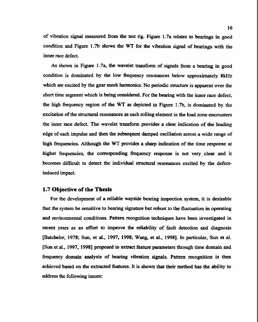
The Wavelet Transform 0, on the other hand, is similar to the STFT in that it also
provides a time-frequency map of the signal being analyzed. The improvement that the
WT makes over the STFT is that it can achieve high frequency resolutions with sharper
time resolutions. Figure 1.7 shows the continuous wavelet transform of 10.2 milliseconds
16
of vibration signal measured from the test rig. Figure 1.7a relates to bearings in good
condition and Figure 1.7b shows the WT for the vibration signal of bearings with the
inner race defect.
As shown in Figure 1.7% the wavelet transform of signals from a bearing in good
condition is dominated by the low fkquency resonances below approximately 8kHz
which are excited by the gear mesh harmonics. No periodic structure is apparent over the
short time segment which is being considered- For the bearing with the inner race defect,
the high frequency region of the WT as depicted in Figure 1.7b, is dominated by the
excitation of the structural resonances as each rolling element in the load zone encounters
the inner race defect The wavelet transform provides a clear indication of the leading
edge of each impulse and then the subsequent damped oscillation across a wide range of
high freguencies. Although the WT provides a sharp indication of the time response at
higher frequencies, the corresponding fiequency response is not very- clear and it
becomes difficult to detect the individual structural resonances excited by the defect-
induced impact.
1.7 Objective of the Thesis
For the development of a reliable wayside bearing inspection system, it is desirable
that the system be sensitive to bearing signature but robust to the fluctuation in operating
and environmental conditions. Pattern recognition techniques have been investigated in
recent years as an effort to improve the reliability of fault detection and diagnosis
patchelor, 1978; Sun, et al., 1997, 1998; Wan& et al., 19981. In particular, Sun et al.
[Sun et al., 1997, 19981 proposed to extract feature parameters through time domain and
frequency domain analysis of bearing vibration signals. Pattern recognition is then
achieved based on the extracted features. It is shown that their method has the ability to
address the following issues:
17
1) Severity of the bearing damage: This is realized by using feature parameters
representing the vibration energy levels due to increased bearing damage;
2) Robusmess to bearing loads and rotating speeds: Such time domain parameters as
Peak and RMS values are normalized by the baseline RMS values representing
good bearings. Through in-line measurement of bearing vibrations, the baseline
RMS value is obtained by averaging the vibration signals over all the bearings
mounted on the freight train. It counteracts the effect of fluctuating bearing loads
and rotating speeds, as well as environment conditions;
3) Location of bearing fatigue spalls: Frequency index was proposed to capture the
dominant vibration components in the spectrum that may be associated with
particular bearing characteristic kquencies. The latter can be used to identify the
location of bearing defects.
Above all, their method is shown to be simple to implement and does not require human
operator's knowledge of signal analysis. This is an important feature when it comes to the
development of automatic diagnosis systems. In this thesis, we intend to pursue further
improvement on the pattern recognition technique proposed by Sun et al. Two endeavors
will be attempted along the same h e . Firstly, more feature parameters will be
investigated to highlight the time and frequency relations according to the bearing
dynamics. The purpose is to further improve the sensitivity and reliability of the
technique. This will be achieved through segmentation analysis. Secondly, a nonlinear
mapping between the feature space and the classification space will be explored for the
purpose of dimension reduction to facilitate piecewise linear class~cations. In [Sun, et
al., 19981, a linear projection based on the least squared principle is applied. This must be
followed by intra-class transformation due to the poor performance of the linear mapping.
In order for the linear classification to be applicable, successful mapping is considered
18
when data points belonging to the same class are clustered together without overlapping
other classes in the classification space. A multi-layered artificial neural network will be
investigated for use in performing the high fidelity dimension reduction nonlinear
mapping. The intra-class transformation can be eliminated thereby.
The same experimental data as used by Sun et a1 will be used. Studies will also be
conducted to compare the results and show the improvements achieved by this work.
1.8 Organization of the Thesis
The thesis is organized into six chapters. In chapter 2, bearing structure, kinematics
and vibration models are described. An understanding of bearing geometry and
kinematics is essential for bearing fault detection as it determines the bearing defect
characteristic frequencies. Vibration models of localized fatigue spalling are also
presented in this chapter.
Chapter 3 focuses on feature extraction to construct the feature space for the pattern
recognition of bearing conditions. Vibration signals obtained fkom bearings are digitized
and processed through time domain, fkquency domain and segmentation analyses. Time
domain analysis can be conducted by calculating the statistical parameters and the energy
level of the vibration signals. Frequency domain are also introduced. The
newly developed parameters based on segmentation analysis are presented as well.
In chapter 4, artificial neural networks are discussed. They are used to perform the
nonlinear mapping from the feature space to the classification space. The basic
architecture of artificial neural networks is discussed, with a focus on the multi-layered
feedforward ANNs. The error back-propagation training algorithm is explained in detail.
The convergence speed, stopping criteria and adjustment of initial and cumulative
weights of the neural network are also discussed. The optimal architecture employed for
19
the ANN used in this work is presented. The learning-rate adaptation theory and its
application to convergence improvement are also discussed.
Chapter 5 presents experimental studies. A total number of 115 samples provided by
AAR were used for training. A total number of 3 1 test data (not used in training) from
bearings with defects of different types were used to test the effectiveness of the
developed method. Comparisons were made with and without the segmentation
parameters. It is shown that segmentation parameters increase the sensitivity and
therefore the reliability and efficiency of the pattern recognition technique.
Chapter 6 concludes the thesis with a summary of the results obtained, a discussion of
the limitations of the proposed methods, and proposes some directions for W e work.
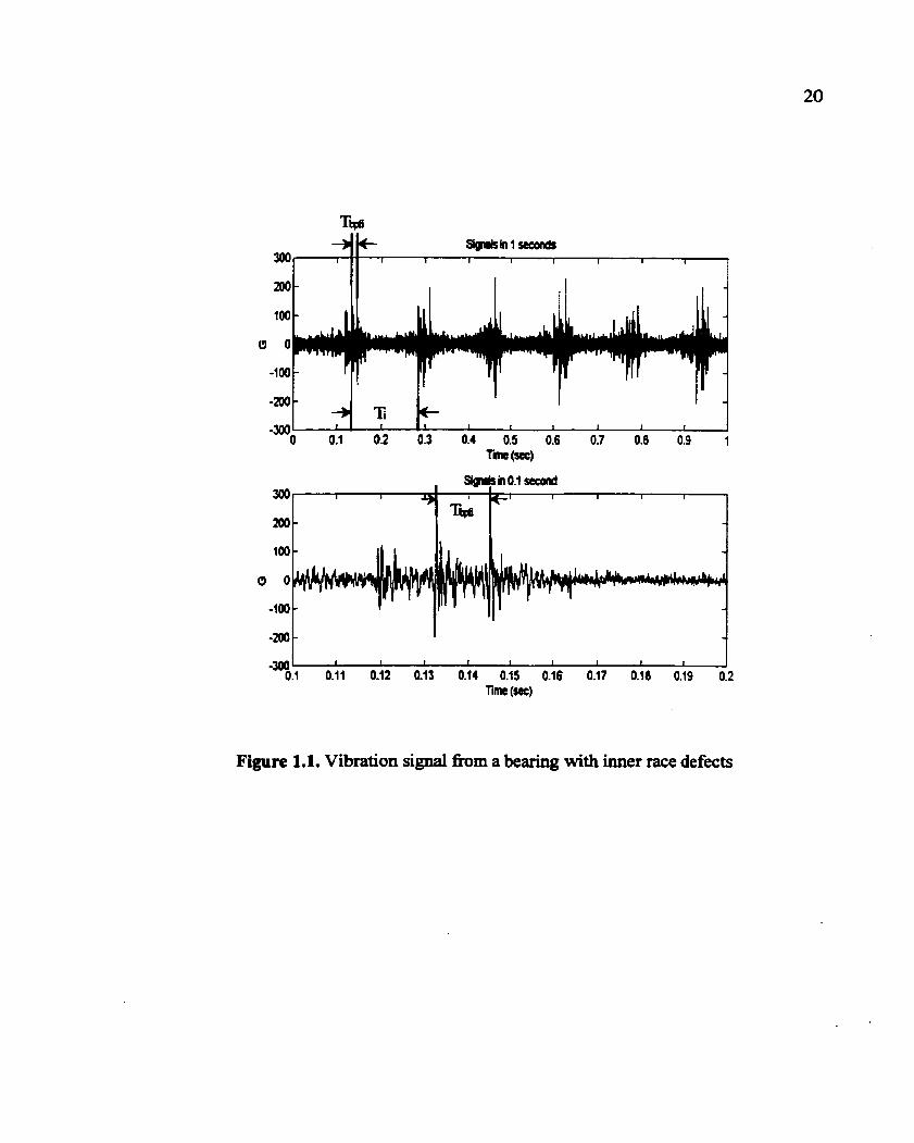
Figure 1.1. Vibration signal h m a bearing with inner race defects
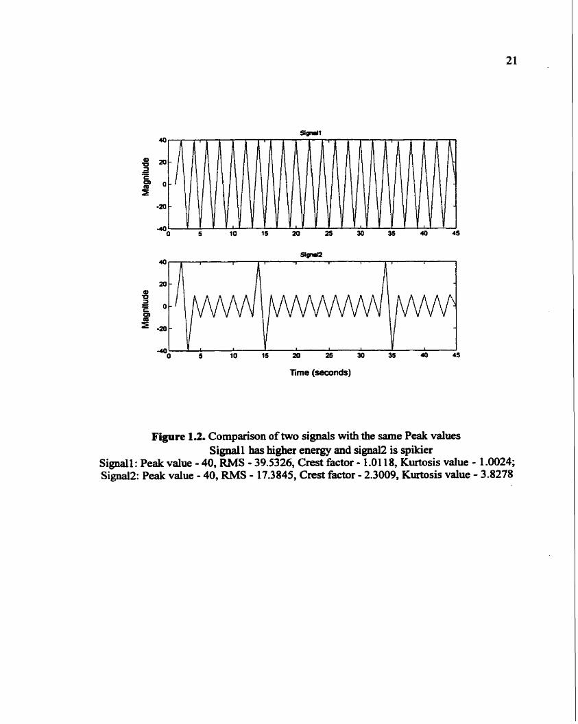
Figure 1.2. Comparison of two signals with the same Peak values Signall has higher energy and signal2 is spikier
Signall: Peak value - 40, RMS - 39.5326, Crest factor - 1.01 18, Kurtosis value - 1.0024; Signal2: Peak value - 40, RMS - 17.3845, Crest factor - 2.3009, Kurtosis value - 3.8278
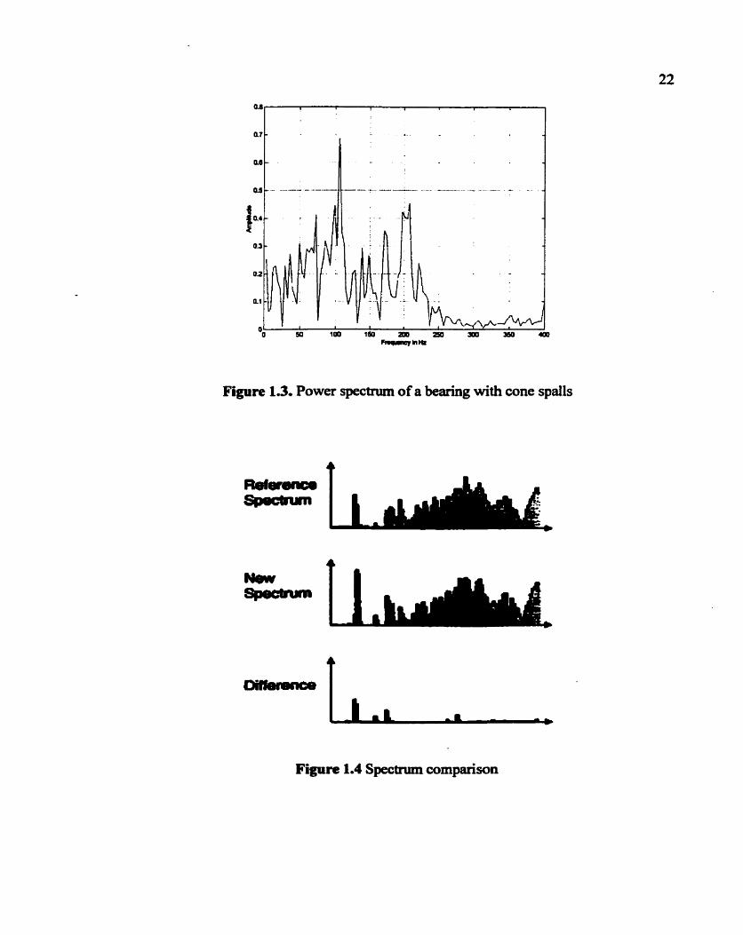
Figure 1.3. Power spectrum of a bearing with cone spalls
Figure 1.4 Spectrum comparison
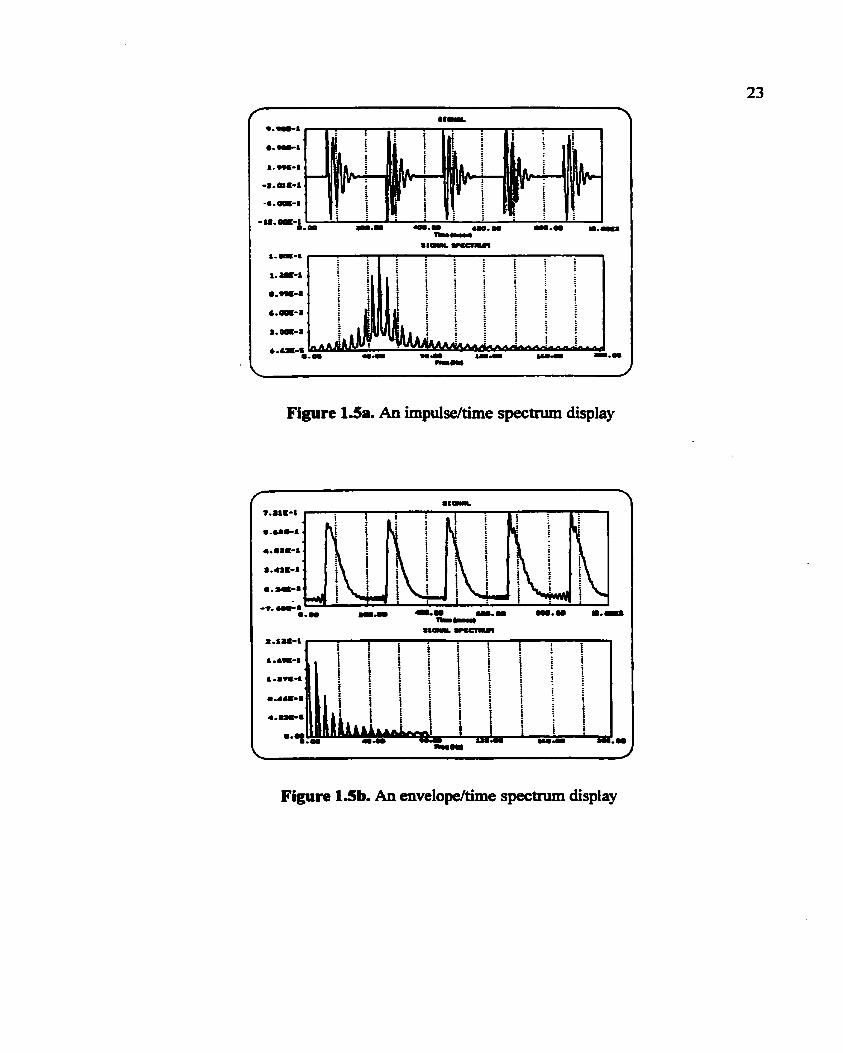
Figure 1-5% An impulse/time spectrum display
Figure 1.5b. An envelopehime spectnun display
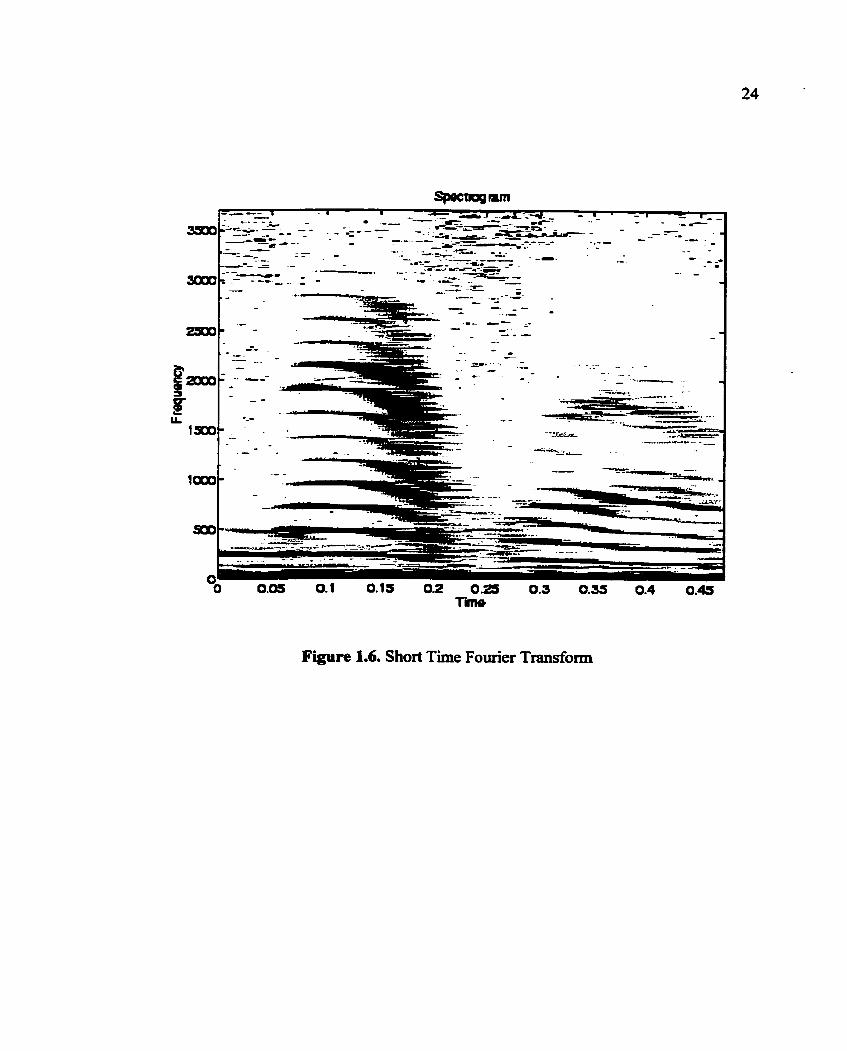
Figure 1.6. Short Time Fourier Transform
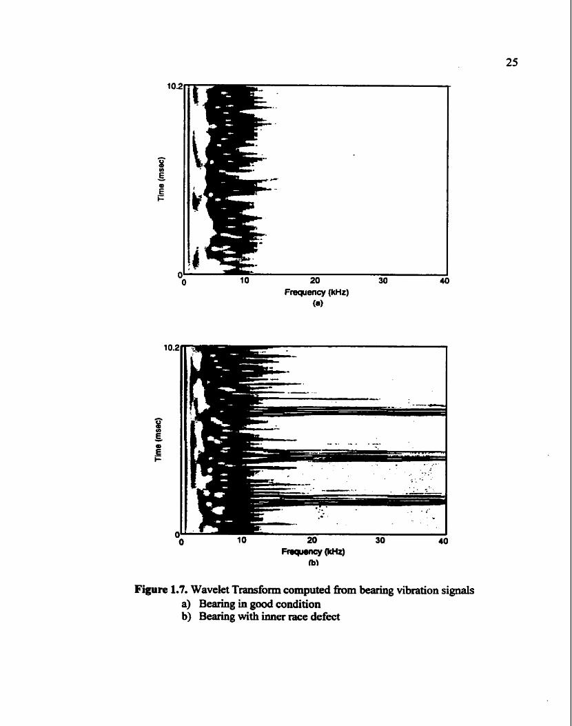
Fiyre 1.7. Wavelet Transform computed h m bearing vibration signals a) Bearing in good condition b) Bearing with inner race defect
CHAPTER TWO
BEARING KINEMATICS
2.1 Bearing Structure
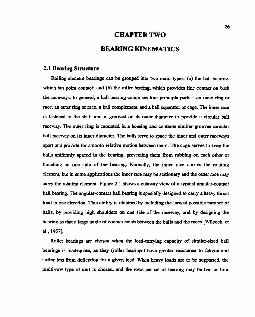
Rolling element bearings can be grouped into two main types: (a) the ball bearing,
which has point contact; and @) the roller bearing, which provides line contact on both
the raceways. In general, a ball bearing comprises four principle parts - an inner ring or
race, an outer ring or race, a ball complement, and a ball separator or cage. The inner race
is fastened to the shaft and is grooved on its outer diameter to provide a circular ball
raceway. The outer ring is mounted in a housing and contains similar grooved circular
ball raceway on its inner diameter. The balls serve to space the inner and outer raceways
apart and provide for smooth relative motion between them. The cage serves to keep the
balls uniformiy spaced in the bearing, preventing them h m rubbing on each other or
bunching on o w side of the bearing. Normally, the inner race carries the rotating
element, but in some applications the inner race may be stationary and the outer race may
carry the rotating element. Figure 2.1 shows a cutaway view of a typical angular-contact
ball bearing. The angular-contact ball bearing is specially designed to carry a heavy thrust
load in one direction. This ability is obtained by including the largest possible number of
b d s by providing high shoulders on one side of the raceway, and by designing the
bearing so that a large angle of contact exists between the balls and the races [Wilcock, et
al., 19571.
Roller bearings are chosen when the loadcarrying capacity of similar-sized ball
bearings is inadequate, as they (roller bearings) have greater resistance to fatigue and
suffer less fiom deflection for a given load. When heavy loads are to be supported, the
multi-row type of unit is chosen, and the rows per Jet of bearing may be two or four
[Houghto~~ 19651. Similarly, a roller bearing consists of four principle elements - an
inner race, an outer race, a complement of rollas, and a separator or cage for the rollers.
In some cases, the inner race is made an integral part of the shaft instead of a separate
member which is mounted on the shaft. The outer race is normally mounted in a
stationary housing, although occasionally the inner race may be stationary while the outer
race rotates. The rollers and the cage perform similarly with the balls and the cage of ball
bearings.
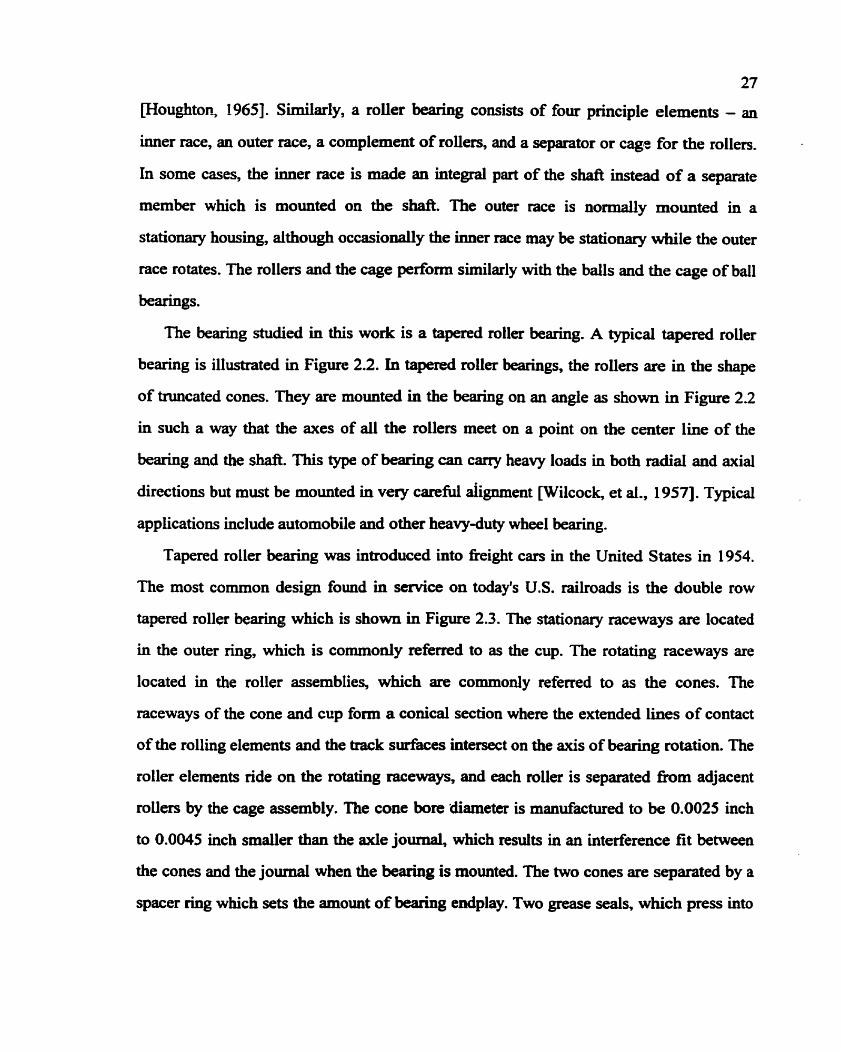
The bearing studied in this work is a tapered roller bearing. A typical tapered roller
bearing is illustrated in Figure 2.2. In tapered roller bearings, the rollers are in the shape
of truncated cones. They are mounted in the bearing on an angle as shown in Figure 2.2
in such a way that the axes of al l the rollers meet on a point on the center line of the
bearing and the shaft. This type of bearing can carry heavy loads in both radial and axial
directions but must be mounted in very carefbl alignment [Wilcock, et al., 1 9571. Typical
applications include automobile and other heavy-duty wheel bearing.
Tapered roller bearing was introduced into fieight cars in the United States in 1954.
The most common design found in service on today's U.S. railroads is the double row
tapered roller bearing which is shown in Figure 2.3. The stationary raceways are located
in the outer ring, which is commonly referred to as the cup. The rotating raceways are
located in the roller assemblies, which are commonly referred to as the cones. The
raceways of the cone and cup form a conical section where the extended lines of contact
of the rolling elements and the track surfaces intersect on the axis of bearing rotation. The
roller elements ride on the rotating raceways, and each roller is separated from adjacent
rollers by the cage assembly. The cone bore 'diameter is manufactured to be 0.0025 inch
to 0.0045 inch smaller than the axle journal, which tesults in an intefference fit between
the cones and the journal when the bearing is mounted. The two cones are separated by a
spacer ring which sets the amount of bearing endplay. Two grease seals, which press into
28
the cup and ride on the wear rings, act to retain the bearing lubricant and prevent
lubricant contamhation. The bearing is held in place on the axle journal by an end cap
assembly which includes three cap screws.
2.2 Bearing Kinematics
Because the contacts between defects and the mating surfaces in the bearing are
essentially periodic, impulses will recur at regular intervals. The frequency of occurrence
of impulses is referred to as the characteristic defect fkquency.
Resonance is usually considered as being amplitude modulated at the characteristic
defect hquency. This is not sinusoidal modulation, as the leading edge comprises a very
sharp rise corresponding to the impact of the defect, while the decay is approximately
exponential, as the energy is dissipated by internal damping. The end result consists of
periodic bursts of exponentially decaying sinusoidal vibration. The frequency of the
vibration is the natural fkequency of the resonance, while the decay rate is determined by
the damping WcFadden, et al., 1984bJ.
An understanding of bearing geometry and kinematics is essential for bearing fault
detection as it determines the rotational speeds of the bearing elements with respect to
each other and the theoretical bearing defect characteristic frequencies.
A number of articles deal with bearing geometry and kinematics [Gustafsson, et al.,
1962; Howard, 19941. Figure 2.4 shows a schematic of a typical angular contact rolling
element bearing in the general case with rotating inner and outer races.
From the geometry, assuming a constant operating contact angle a, the pitch circle
diameter of the bearing D can be approximated by,
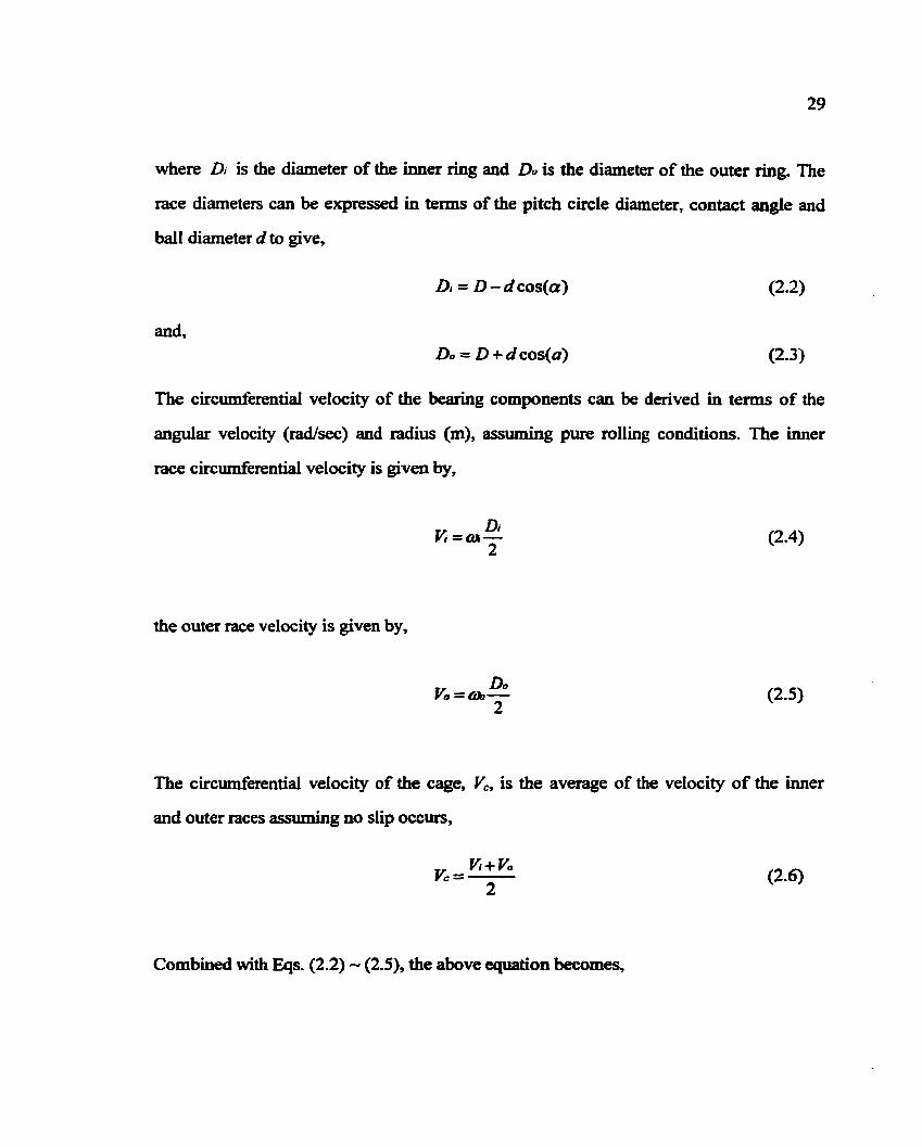
where Dj is the diameter of the inner ring and DO is the diameter of the outer ring. The
race diameters can be expressed in terms of the pitch circle diameter, contact angle and
ball diameter d to give,
The circderentid velocity of the bearing components can be derived in terms of the
angular velocity (rad/sec) and radius (m), assuming pure rolling conditions. The inner
race circumferential velocity is given by,
the outer race velocity is given by,
The circumferential velocity of the cage, V , is the average of the velocity of the inner
and outer races assuming no slip occurs,
Combined with Eqs. (2.2) - (2.5), the above quation becomes,
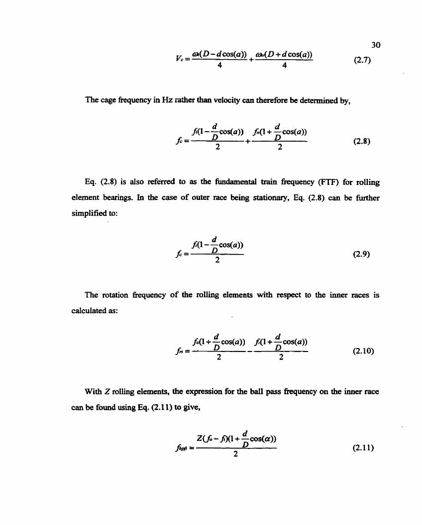
The cage kquency in Hz rather than velocity can therefore be determined by,
Eq. (2.8) is also referred to as the hdamental train hquency (FTF) for rolling
element bearings. In the case of outer race being stationary, Eq. (2.8) can be further
simplified to:
The rotation fkequency of the rolling elements with respect to the inner races is
calculated as:
With Z rolling elements, the expression for the b d pass kquency on the inner race
can be found using Eq. (2.1 1) to give,
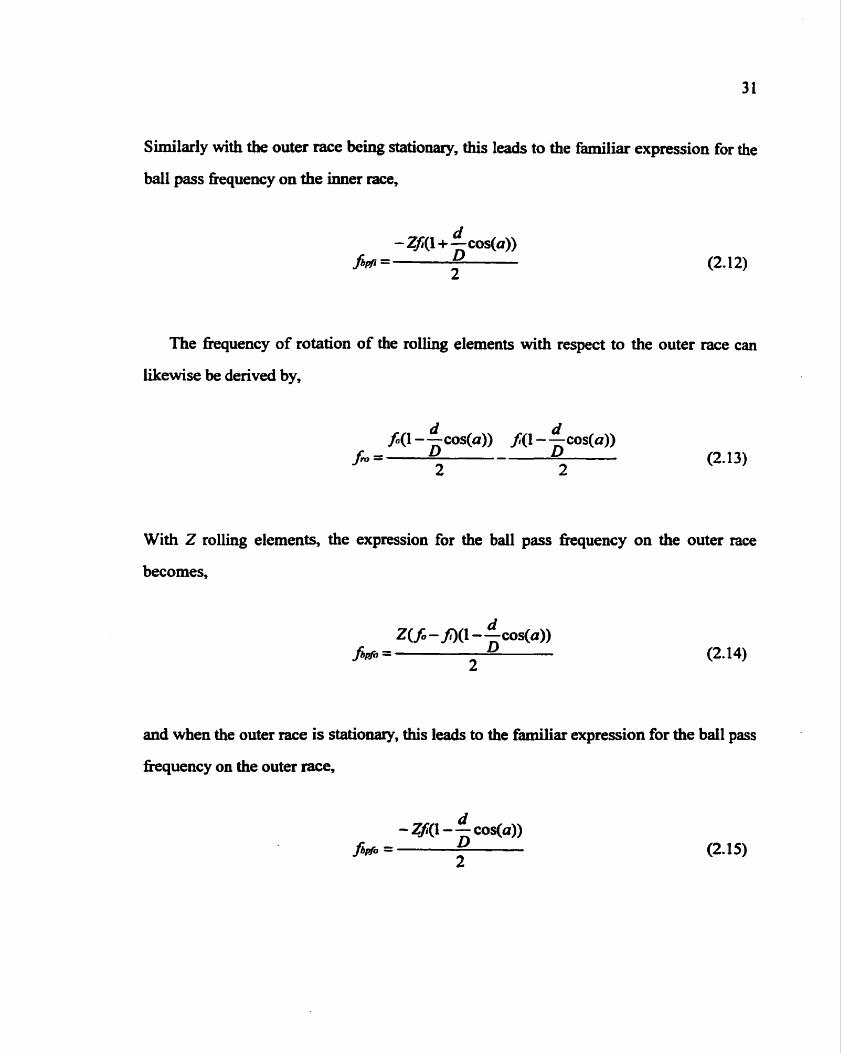
Similarly with the outer race being stationary, this leads to the familiar expression for the
ball pass frepuency on the inner race,
The frequency of rotation of the rolling elements with respect to the outer race can
likewise be derived by,
With Z rolling elements, the expression for the ball pass fkquency on the outer race
becomes,
and when the outer race is stationary, this leads to the familiar expression for the ball pass
fkquency on the outer race,
32
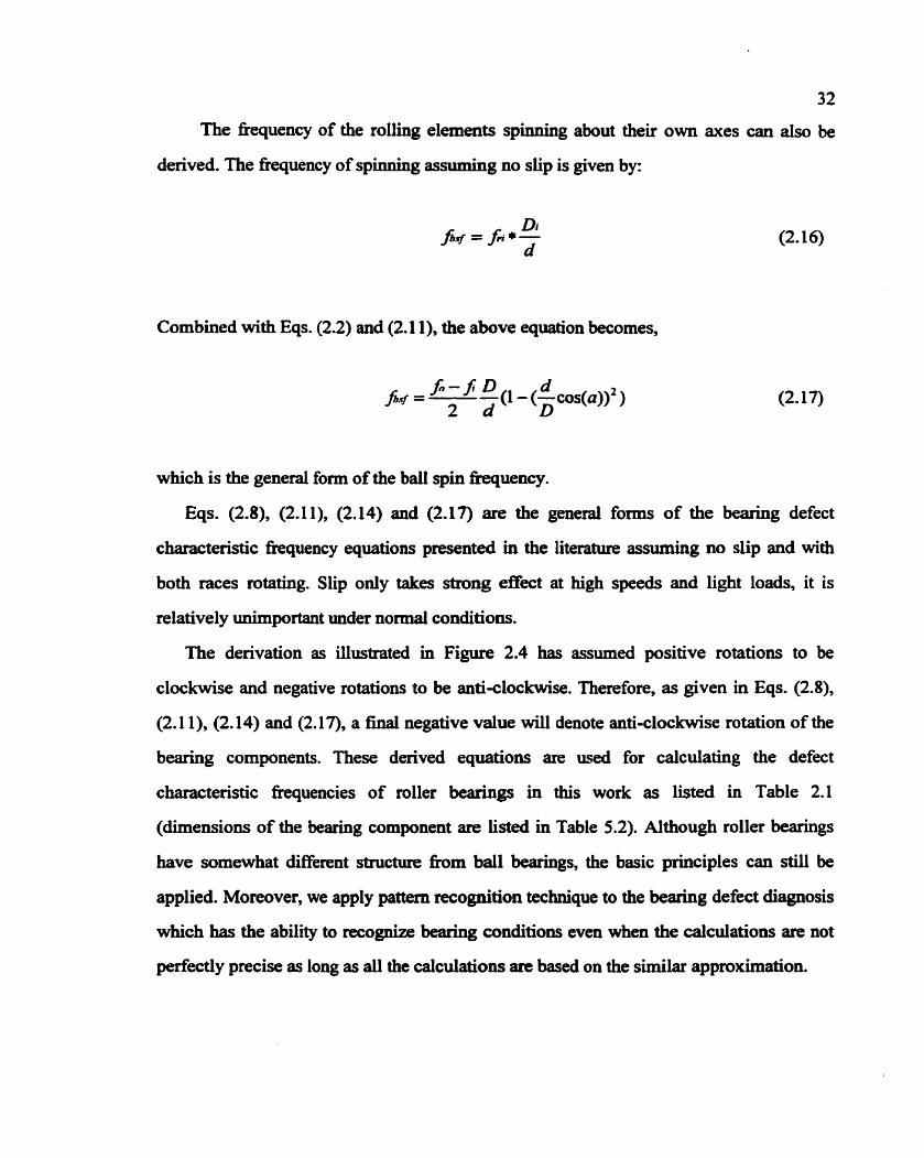
The fkequency of the rolling elements spinning about their own axes can also be
derived. The frequency of spinning assuming no slip is given by:
Combined with Eqs. (2.2) and (2.1 I), the above equation becomes,
which is the general form of the ball spin kquency.
Eqs. (2.8), (2.1 l), (2.14) and (2.17) are the general forms of the bearing defect
characteristic fkquency equations presented in the literature assuming no slip and with
both races rotating. Slip only takes strong effect at high speeds and light loads, it is
relatively unimportant under normal conditions.
The derivation as illustrated in Figure 2.4 has assumed positive rotations to be
clockwise and negative rotations to be anti-clockwise. Therefore, as given in Eqs. (2.8),
(2.1 I), (2.14) and (2.17), a final negative value will denote anti-clockwise rotation of the
bearing components. These derived equations are used for calculating the defect
characteristic hquencies of roller bearings in this work as listed in Table 2.1
(dimensions of the bearing component are listed in Table 5.2). Although roller bearings
have somewhat different structure &om ball bearings, the basic principles can sti l l be
applied. Moreover, we apply pattern recognition technique to the bearing defect diagnosis
which has the ability to tecognize bearing conditioos even when the calculations are not
perfectly precise as long as all the calculations are based on the similar approximation.
33
2.3 Vibration Models of Localized Fatigue Spalling
The bearing kquency equations provide a theoretical estimate of the frequencies to
be expected when various defects occur on the bearing elements, based upon the
assumption that an ideal impulse will be generated whenever a bearing element
encounters the defect. Impulses are generated when localized bearing defects such as
fatigue spa11 occurs on the bearing components. The initial model of the vibration
generation mechanism was developed by McFadden WcFadden, et al., 1984al. It
considers the vibration produced as the rolling elements encounter the defect to consist of
a series of impulses representing the transient force imbalance to the machine structure.
As the shaft rotates, the impulses occur periodically with the characteristic frequencies
depending on the location of the defect. Defects on the inner race of a bearing with a
stationary outer race were considered assuming the bearing is operating under radial
loads. The resulting modulation of the impulses with shaft rotation as the defect rotates in
and out of the load zone was considered. By considering the response of a typical
structural resonance, the vibration measured fiom each impulse was assumed to take the
form of an exponentially decaying sinusoid. The resulting vibration as measured by the
transducer was shown to be a combination of the periodic impulses, modulation due to
rotation through the load zone and the exponential decay of the impulses due to internal
structural damping. The complete model was experimentally verified for an inner race
defect. Vibrations measured fiom a bearing test rig confirmed that for inner race localized
defects the predominant features consist of sh& fkquency harmonics, the ball pass
frequency on the inner race&¶ modulated by shaft kquencies, and multiple harmonics
thereof.
Su, et al [Su, et al., 19921 extended the original work by McFadden to characterize
the vibrations measured fiom bearings subjected to various loading conditions and with
defects located on various bearing components. The main development of the work was
34
the determination of the periodic characteristics of various loading and its influence on
the vibration. The effect is generally associated with the misalignment or dynamic
unbalance of the shaft the axial or radial loading, the preload and manufacturing
imperfections.
Su's work presented the main causes of periodicities and the resulting effect of
defects on the various bearing components. For a roller defect, the vibration pattern
produced is in some respects similar to that produced by a bearing with an inner race
defect as discussed above. The defective roller revolves with the cage frequency and the
defect contacts the inwr and outer race alternately. The relative angular frequencies
between the defective roller and the load will be the cage frequency&. The contact point
for the defect will move alternately from the inner race to the outer race at twice of the
ball spin fiequency 2x& Thus the predominant features in the vibration consist of cage
frequency harmonics, the roller defect frequencies, modulated by cage frequencies, and
multiple harmonics thereof.
For an outer race spall, with fixed outer race, the damage site remains in a fixed
position relative to distribution of load around the bearing. The resulting vibration will
not be modulated with either the shaft frequency& or the cage frequency/,. The impulses
occur periodically with the ball pass frequency on the outer race fipfo. However, if the
shaft has unbalance or the rollers have diameter errors, the periodic variation will occur
with the shafl fiequencyf, due to unbalance rotating at the shaft frequency or the cage
fiequencyf, due to a non-uniform load distribution rewolving with the cage assembly.
Having obtained a model to predict the possible bearing frequencies and harmonics
for the various types of localized fatigue damage, the pattem of expected fkequencies can
be searched for as part of routine bearing condition monitoring. Further work has shown
that the analysis of the magnitude of the defect frequencies relative to each other
improves reliability [Su, et al., 19931.
35
The modelling of bearing defects other than localized spalling has received little
attention. The relevant fkquencies which can occur are not readily apparent or
necessarily static in time. This makes detection and diagnosis of bearing damage using
frequency analysis difEcuit for all but the straightforward cases of fatigue spalling. In this
work, we focus on the localized bearing spaUing caused by fatigue. These widely
accepted vibration models prompt the development of some distinctive features which
will be detailed in chapter 3.
Figure 2.1 Angular-contact ball bearing
Figure 23 Tapered roller bearing
on CONe OR CUP
Figure 23 Standard kight car rolling bearing
Figure 2.4 Schematic of a rolling element angular contact bearing
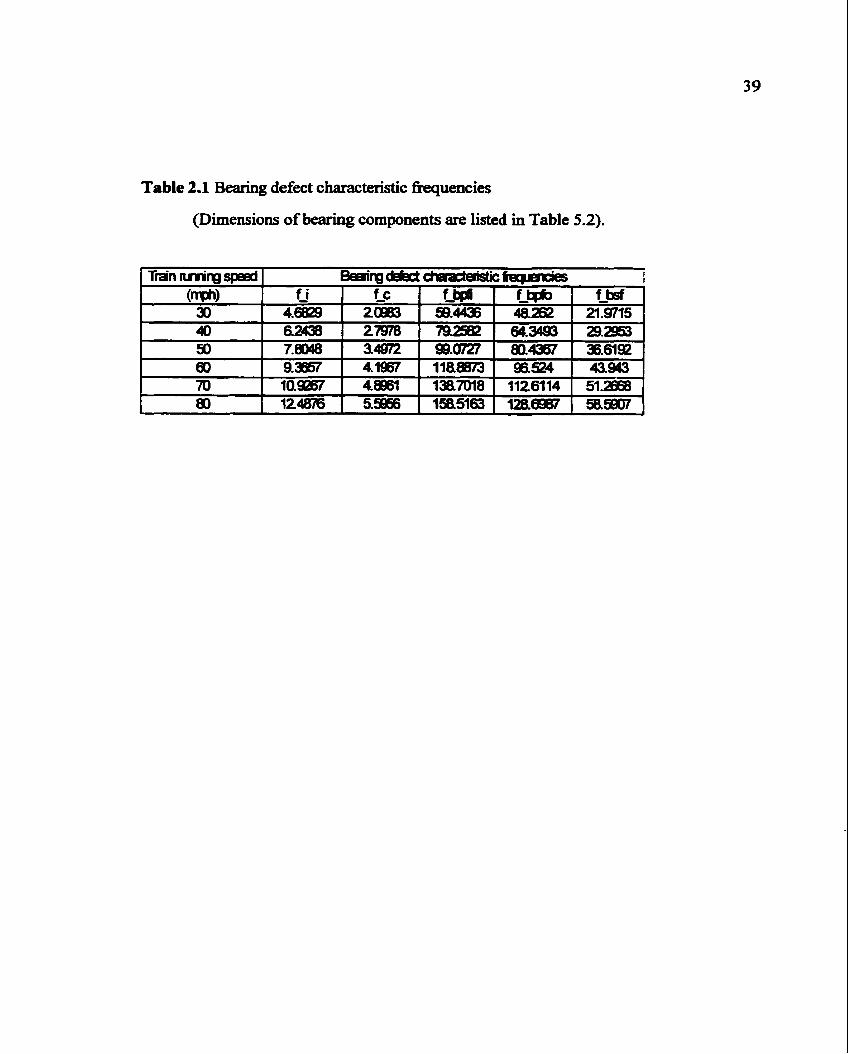
Table 2.1 Bearing defect characteristic kquencies
(Dimensions of bearing components are listed in Table 5.2).
CHAPTER THREE
FEATURE EXTRACTION FOR PATTERN RECOGNITION
3.1 Feature Ex~baction
One of the greatest problems encountered when applying pattern recognition
techniques to the analysis of vibration signals is deciding on the method of feature
extraction to be used. Extracting feature parameters from the measured data is most
critical for effective fault detection and diagnosis pnal, 19941. Diagnostics based on
pattern recognition become more efficient and precise if correct feature parameters are
employed. Therefore, feature extraction becomes a very crucial component. In feature
e m t i o n , the knowledge of the real system dictates the number of the feature space
dimensions. In other words, the better the system is known, the easier its monitoring and
diagnostics will be.
Ideally, features are selected so that they uniquely represent certain characteristics
of the system. However, the challenge lies in the fact that it is not always straightforward
how to select the feature panuneters. It also depends on the system we are dealing with.
Therefore, it is also desirable that the selected features are robust to noise and operating
conditions. In dealing with vibration signals, features can be extracted using various
signal processing techniques, such as time domain and fkquency domain analyses.
3.2 Time Domain Parameters
When fauit occurs in a bearing, abnormal behavior can be seen h m the vibration
signals, e.g. sharp impulses for incipient damages and higher energy level for more
developed defects. Figure 3.l(a, b) show vibration signals taken h m a bearing in good
condition and with defects nspectively. It can be seen that the vibration amplitude of the
41
defective bearing is much higher than the bearing in good condition. Time domain feature
extraction can be conducted by calculating the statistical parameters, which provides
information about probability density distribution that can indicate the spikiness of the
signal associated with the defect induced impulses. Peak and Root Mean Square values
are also included to indicate the severity of bearing defects [Sun, et al., 19991. These
parameters prove to be simple and effective in identifying bearing fault cawed by fatigue
spalls [Sun, et al., 1998; Sun, et al., 19991.
3.2.1 Probability Density Function
Local discontinuity of the material on the surface of bearing raceways or rolling
elements produces a series of impulses in vibration signals which can be modulated with
the bearing rotation and superimposed onto a random background vibration. Due to
damping in the bearing material and fluids, impulse signals quickly decay in time until
next impulse is generated. Patterns exist that can be associated with the location and
severity of the fatigue spalls. For instance, on-set defects tend to generate clean and
spikier impulses. Frequencies of these impulses could help identifying the location using
characteristic frequency calculations introduced in chapter 2.
The amplitude characteristics of a vibration signal X(t) (assumed to be a stationary
random process) can be expressed in terms of a probability density hc t ion (PDF) m e r ,
et al., 1978; Alfiedson, et al., 1985b; Bannister, 1985; Mathew, 19891. This is estimated
by determining the time duration for which a signal remains in a set of amplitude
windows.
A t i P ( X S x(t)s x + ~ ) = C -
r-I T
42
Where A t i is the time duration of the vibration signal X(t) falling into the amplitude
window hx . T is the total time duration of the vibration signal.
The above equation for all x with &small, results in an estimate of probability
function for X(t) (at selected life times) shown in Figure 3.2. The PDF of a good bearing
and a defective bearing are represented by the solid line and the dashed line respectively.
It can be observed that a good bearing with random vibrations has a Gaussian
distribution, while changes in the distribution curve, particularly at the lower values of
the PDF, indicate early stages of bearing failure. Note that a logarithmic scale was used
for the vertical axis to highIight the behavior at the extreme limits of the distributions,
such as the changes at low probability which have been found important in detection of
bearing damage. The horizontal axis is the acceleration of the vibration signal normalized
to the standard deviation.
Probability density curve derived from machinery vibration signals can be used in
monitoring machine conditions. It has been shown that the normalized PDF of the
vibration signal does not vary with load aud speed but changes as the condition of a
bearing deteriorates [Li, et al., 19921. With advancing damage the tails of the PDF
initially broaden. The high levels of probability density at the median and the large
spread at low probabilities, are characteristics of highly impulsive time domain
waveforms [Mathew, 19891. It is possible to quantify the variations in the skia of the
probability distribution by taking statistical moments which will be discussed in section
3.2.3. However, when the pitting and subsequent spalling has spread over most of the
working surfaces of the rolling element bearings, the probability density returns to the
basic Gaussian form once again bi, et al., 19921.
43
3.2.2 Root Mean Square and Peak Value
Root Mean Square (RMS) is often used to indicate the energy level of vibrations.
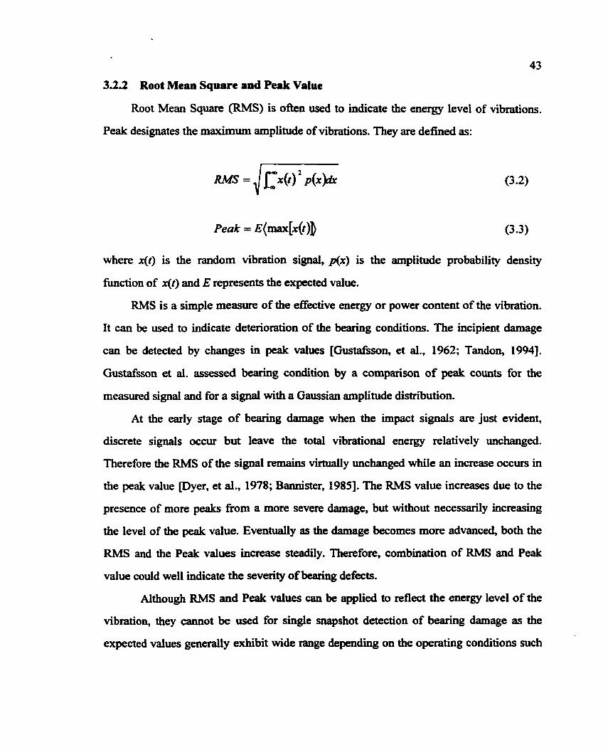
Peak designates the maximum amplitude of vibratious. They are defined as:
Peak = ~(max[x ( t ) )
where x(t) is the random vibration signal, p(x) is the amplitude probability density
k c t i o n of x(t) and E represents the expected value.
RMS is a simple measure of the effective energy or power content of the vibration.
It can be used to indicate deterioration of the bearing conditions. The incipient damage
can be detected by changes in peak values pustafbson, et al., 1962; Tandon, 19941.
Gustafsson et al. assessed bearing condition by a comparison of peak counts for the
measured signal and for a signal with a Gaussian amplitude distribution.
At the early stage of bearing damage when the impact signals are just evident,
discrete signals occur but leave the total vibrational energy relatively unchanged.
Therefore the RMS of the signal remaim virtually unchanged while an increase occurs in
the peak value [Dyer, et al., 1978; Bannister, 19851. The RMS value increases due to the
presence of more peaks fkom a more severe damage, but without necessarily increasing
the level of the peak value. Eventually as the damage becomes more advanced, both the
RMS and the Peak values increase s t m y . Therefore, combination of RMS and Peak
value could well indicate the severity of bearing defects.
Although RMS and Peak values can be applied to reflect the energy level of the
vibration, they cannot be used for single snapshot detection of bearing damage as the
expected values generally exhibit wide range depending on the operating conditions such
44
as load and speed and the testing environment. Unless the measured values of RMS and
Peak can be compared with the baseline values for a system under the same operating
conditions, they cannot be used effectively. For railway applications it is particularly
difficult to determine the baseline of the beating fiom a single measurement since no
particular information about the operating conditions of the passing freight car is
available.
Sun, et al, proposed to use normalized values of Peak and RMS to take into
account the operational condition and non-defect induced vibrations:
where RMSo is considered as the reference value for an undamaged bearing. There are
different ways of obtaining this value depending on the specific application. For bearing
used in fixed machinery, RMSo could be the value taken when the bearings are in good
condition and under ordinary operating conditions. For railway bearing condition
monitoring, RMSo could be the average of the RMS values of all the signals taken fiom
all the bearings passing by the sensor.
3.2.3 Statistical Parameters
Time domain statistical parameters have been used as one-off and trend parameters
in an attempt to detect the presence of incipient bearing damage. The commonly used
non-dimensional vibration amplitude parameters are the Crest factor (Cf), Kurtosis
value(Kv), Impulse factor (If) and Clearance fhctor (Clf) ~oward , 19941. These
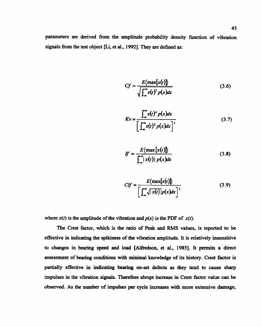
45
parameters are derived from the amplitude probability density function of vibration
signals from the test object [Li, et al., 19921. They are defined as:
where x(t) is the amplitude of the vibration andp(x) is the PDF of x(f).
The Crest factor, which is the ratio of Peak and RMS values, is reported to be
effective in indicating the spikiness of the vibration amplitude. It is relatively insensitive
to changes in bearing speed and load [Akedson, et al., 19851. It pennits a direct
assessment of bearing conditions with minimal knowledge of its history. Crest factor is
partially effective in indicating bearing on-set defects as they tend to cause sharp
impulses in the vibration signals. Therefore abrupt increase in Crest factor value can be
observed. As the number of impulses per cycle increases with more extensive damage,
46
the RMS value increases while the Peak value remains unchanged. The net effect is that
the Crest factor will decrease.
A series of statistical moments can be used to indicate the shape of the probability
density distribution Flathew, 19871. These can be defined by the following integral
IPyer, et al., 19781:
where n represents the order of the statistical moment, m is the maximum order under
consideration. The first and second moments are known as the mean value and the
standard deviation respectively. These are analogous to the first and second area
moments of inertia with the area shape defined by the probability density hction. The
third moment is Skewness and the fourth moment is Kurtosis. For practical signais the
odd order moments are usually close to zero, indicating a symmetrical amplitude
distribution, whereas the higher even order moments are sensitive to the impulsiveness in
the signal.
The fourth moment Kurtosis value has been selected as a feature parameter in this
work since it is a compromise measure between the insensitive lower moments and the
over-sensitive higher moments. It has a value of 3.0 for an undamaged bearingy indicating
a Gaussian probability density function. A value of as high as 6.0 can be used to s i m
incipient bearing damage, indicating that the skirt of the PDF has changed appreciably
and is no longer Gaussian.
Similar to the Crest factor, the advantage of employing Kurtosis is that it is robust
to bearing operating conditions. This parameter is reported to be sensitive to failure in
47
rolling element bearings [Dyer, et al., 19781. In this case, cracked raceways and rolling
elements can cause large impulses in the time domain waveform.
Both Crest factor and Kurtosis value are independent of the actual magnitude of the
vibration but respond more to the spikiness of the vibration signal. These two parameters
produce values of approximately 3.0 which indicate that the waveform is generally
random in nature when the bearing is in good condition. They will increase dramatically
when fatigue spa11 is introduced. However, progression of the damage does not make
them increase continuously.
For instance, in the case of inner race defect, the circumferential extent of the crack
is much less than the distances between two rollers at the early stage when fatigue spa11 is
just developed. The system is excited by discrete shock loads. As damage propagates and
spreads around the periphery of the loading region of the bearing, vibration pattem
becomes more random. The impulsive content in the waveform gradually decreases and
the vibration signal appears to be continuous. Crest factor and Kurtosis value will then
reduce to normal in all frequency ranges. Therefore, these two parameters alone cannot
provide direct information on the severity of the bearing damage. Noting that significant
increase of overall vibration energy often accompanies more severe damage, a
combination of these two parameters and RMS value should be applied simultaneously.
This motivates us to develop the pattem recognition technique.
Impulse and Clearance factors have similar effects as Crest factor and Kurtosis
value [Alguhdigue, et al., 19931. Li and Pickering Ki, et al., 19921 showed that the
Impulse factor (If), Crest factor (Cf), Kurtosis value (Kv) and Clearance factor (Clt) are
all sensitive to early fatigue spalling. Kurtosis value is the most sensitive parameter yet
the least robust, while Clf is most robust to the operating conditions. It shows that these
parameters are sensitive to early spalling but may lead to inconsistent results if used in
isolation.
48
Two approaches can be used to calculate the time domain parameters. The first is to
calculate them for the entire fkquency rauge of the digitized signal, and the second is to
break the signal into various fiequency bands and obtain the parameters for each band. A
number of frequency bands can be chosen for computation and trending of the statistical
parameters. Khan w, 19911 recommended the use of at least two fiequency bands.
One is in the base band dominated by the defect frequencies, low order harmonics and
sidebands (below 5kHt). The other is in the pass band where it will be dominated by
structural resonance of the system (5 - 40kHz). In this work, the aforementioned six time domain parameters, RMS, Peak value,
Crest factor, Kurtosis value, Impulse factor and Clearance factor, are calculated using
two frequency bands: 1) the base band (0-1500Hz) which contains all the bearing
characteristic hquencies at various running speeds; and 2) the pass band (2-lo&)
where vibration signals will be dominated by the structwal resonance. Only one of the
two sets of the six parameters will be retained for constructing the feature space. Either of
the two sets can be used if they have similar values, otherwise the set which deviates
fiom the normal values is used. The time domain parameters computed for the vibration
signals shown in Figure 3.1 are listed in Table 3.1 a. Significant changes can be observed
when fatigue spall occurs on the outer raceway. Table 3.lb shows the time domain
parameters calculated for the same bearing running at different speeds. We can see that
their values also change dramatically at different speeds due to the occurrence of the
defect. It can also be noted that the RMS values (Rv) of the good bearing at different
speeds are all normalized to 1 to provide the references for defective bearings.
3.3 Frequency Domain Parameters
Time domain parameters are useful in detecting defects but they cannot directly
used to indicate the defect's location, e.g. inner race, outer race or the roller.
49
Conventionally, diagnosis of bearing defats and detecting the presence of periodical
components in a signal have been done by anaiyzing the spectrum of the signal. Figure
3.3(a, b) show the fiequency spectra of the vibration signals as shown in Figure 3.l(a, b).
Distinctive peaks can be observed in the fiequency spectrum of the defective bearing
compared to that of the good bearing due to defect-induced impulses.
Contact stresses at the interface between the rollers and the raceways are relatively
high. Abrupt changes in the stress caused by the passage of defects result in impulsive
excitations to the structure. This impulsive force may excite resonance in the bearing and
the housing structure. The excitation decays quickly due to damping of the structure.
Passage on the fatigue spall produces a series of damped oscillations with the time
intervals between the two consecutive peaks corresponding to the time between the
passing of the fatigue spall WcFadden, 19901. The cage frequency&, and ball passing
fiequencies for defects located on the inner race, outer race and rolling elements, denoted
as~p3,fbPI0,fbs/ respectively, can be determined from the bearing kinematics. As discussed
in chapter 2, they are functions of bearing geometry and shaft rotating speed. It is now a
well-established fact that impulsive vibrations can be observed on bearings with fatigue
spall. Therefore, the onset of failure can be detected by noting a predominance at o w of
the passage frequencies such or& Pannister, 19851.
Although the defect characteristic fkequencies could be used to help determine the
location of the defect, automatic detection of impulses at these frequencies is not a simple
task. This is because frequency spectra often show much stronger peaks at much higher
fiequencies representing high order structural resonance compared to those at the
characteristic fkequencies. Vibration energy of the bearing spreads across a wide
fkequeny band and can be easily buried in the noise.
A frequency index (Fi) is proposed to highlight significant fraquency contents that
may be associated with the bearing defat characteristics frequencies [Sun, et al., 19981.
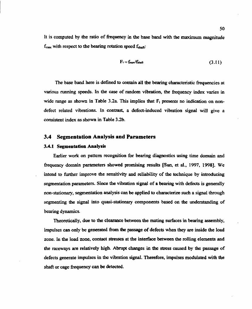
50
It is computed by the ratio of firequency in the base band with the maximum magnitude
f,, with respect to the bearing rotation speed fala:
The base band here is defined to contain all the bearing characteristic frequencies at
various running speeds. In the case of random vibration, the frequency index varies in
wide range as shown in Table 3.2a This implies that Fi presents no indication on non-
defect related vibrations. In contrast, a defect-induced vibration signal will give a
consistent index as shown in Table 3.2b.
3.4 Segmentation Analysis and Parameters
3.4.1 Segmentation Analysis
Earlier work on pattern recognition for bearing diagnostics using time domain and
frequency domain parameters showed promising results [Sun, et al., 1997, 19981. We
. intend to further improve the sensitivity and reliability of the technique by introducing
segmentation parameters. Since the vibration signal of a bearing with defects is generally
non-stationary, segmentation analysis can be applied to characterize such a signal through
segmenting the signal into quasi-stationary components based on the understanding of
bearing dynamics.
Theoretically, due to the clearance between the mating surfaces in bearing assembly,
impulses can only be generated h m the passage of defects when they are inside the load
zone. In the load zone, contact stresses at the interface between the rolling elements and
the raceways are relatively high. Abrupt changes in the stress caused by the passage of
defects generate impulses in the vibration signal. Therefore, impulses modulated with the
shaft or cage fkquency can be detected.
51
Figure 3.4a shows a typical vibration signal recorded from a bearing with inner
race defects. It is obvious that impulses are grouped at the fkequency of the shaft rotation,
and therefore the inner race rotation. If we W e r inspect details of the signal within one
inner race rotation (Figure 3.4b), sharp impacts occurring at the ball passing inner race
frequency can be observed. Furthermore, these impulses only exist in approximately one
third of a complete inner race rotation, which correspond to the period when defects pass
through the load zone of the bearing. This observation contimed our explanation on the
bearing dynamics response.
A schematic of a bearing under radial loads is shown in Figure 3.5, where
raceways, cage and rolling elements are identified. It is also shown in the figure the load
zone with distributed contact stresses over an angular range of about 120°. Defects
located on different bearing components will generate impacts with different frequencies
and modulation patterns when passing through the load zone. Correlation exists between
the location of the defects and the impulse patterns observed in the vibration signal.
Parametric descriptions of various. impulse patterns are possible through segmentation
analysis.
Segmentation of a non-stationary signal can be performed in two ways: fixed
segmentation and adaptive segmentation. A fixed-length segmentation scheme is used in
this work in order to reduce the computational expense of the process. An important
consideration in the fixed segmentation process is the selection of the segment length,
which should reflect both the accuracy and the efficiency. In adaptive segmentation, the
segment length can be decided according to the statistical measure of the signal dynamics
at different time period. The adaptive segmentation may lead to minimum number of
segments however at the expense of increased computational burden of the process. The
autocorrelation function method menstein, et al., 1977; Michael, et al., 19791 uses
52
values of the short-time autocorrelation fbnction to determine the boundaries between
different segments.
To investigate and quantify the impulse patterns of the vibration signal with defects
located at different bearing components, following cases are studied:
Case 1: Inner Race Defect
For bearing with inner race defefts, the distribution of load around the bearing is
often non-uniform as the inner race of the bearing rotates. This is typified by a bearing
under radial load, in which the load around some part of the bearing may be small or, in
the case of a bearing with clearance, even zero. Such a load distribution usually covers a
range of about 120 degrees. The magnitude of the impact produced when a rolling
element strikes a spall will clearly depend on the location of the spall inside the load
zone. As inner race rotates, the magnitude of the defect-induced impacts will vary
periodically with the shaft rotation frequency.
The vibration signal from a bearing with inner race defects is shown in Figure 3.4a.
Obvious variations of the vibration signals in relating to defects inside or outside of the
loading zone can be seen in one revolution corresponding to the rotation of the shaft. If
we divide the signal in one shaft revolution into six segments, at least one segment will
be completely inside the load zone and one completely outside of the load zone (Figure
3.4b). Descriptive features of these segments can be calculated through time domain
parameters, as indicated in Table 3.3a Compared to the values of the parameters for the
bearing in good condition (Table 3.4a), obvious variations of the time domain parameters
among the six segments can be noted, which indicate the existence of defect-induced
impulses. In Table 3.3% most of the values in the last two columns representing the last
two segments in Figure 3.4b are much larger than those in other columns. To capture the
variations among the segments, we decide to calculate the standard deviation of these
53
time domain parameters among six segments and use them as the segmentation
parameters. Table 3.3b shows the values of segmentation parameters for the same bearing
running at different train speeds. Consistent indication can be observed. The low values
of segmentation parameters for the bearing in good condition (Table 3.4b) further
confirm that segmentation analysis is effective in characterizing defect-induced vibration
patterns.
Case 2: Roller Defect
The vibration pattern produced for a roller defect is in some respects similar to that
produced by a bearing with inner race defects. Rollers rotate around the center of the
shaft with the cage at the same time as they spin around their own center axles. When
there is a defect on the roller, it encounters the inner and outer raceways alternately.
Therefore, the relative angular fkquency between the defective roller and the loading is
the cage fkequency. The impact generated &om defects on the roller should be at the
frequency of twice of the ball spin frequency. Figure 3.6a shows the vibration signal
obtained from a bearing with roller defects. Impulses are modulated with the cage
rotation. Figure 3.6b shows the segmentation referenced in one cage revolution. Time
domain parameters are subsequently computed and listed in Table 3.5a It can be
observed that the Peak value and RMS of segment 2 and 3 are higher than those of the
other segments. Table 3.5b shows the segmentation parameters obtained £?om a bearing
with roller defect.
Case 3: Outer Race Defect
Figure 3.7 shows the vibration signal taken h m a bearing with defects on the
outer race. Since the outer race is normally fixed with the bearing housing, defects should
always be initiated and remain inside the load zone. Therefore, defect-induced impulses
54
should not be modulated with either the shaft or the cage rotations. No obvious variation
associated with the shaft or cage rotations can be observed. Still, impacts occurring
periodically with the ball passing outex race characteristic frequencies should be seen
from the signal. Such feature should be captured by the Frequency index as introduced in
our previous work [Sun, et al., 19981. Signals with outer race defects are shown in Figure
3.7a and 3 3 .
Quantitatively, Table 3.6a shows the time domain parameters calculated for the
six signal segments in a single cage revolution. Although no obvious variations of these
parameters exist among different segments, energy level indicated by Rv and Pk for all
segments must be higher for defective bearings. As well, since standard deviation
indicates the absolute difference between the real and the mean values of the signal, it
leads to higher values of m -. and mk -, even though the relative difference is much
less than that in Case 1. Segmentation parameters referenced in the cage frequency of a
bearing with outer race defect at different train speeds are illustrated in Table 3.6b.
3.4.2 Feature Extraction Using Segmentation Parameters
For training and diagnosis purpose, we need to apply the segmentation parameters
mentioned above referenced in both shaft and cage rotations. This is because in
diagnosis, location of the defect is to be determined and therefore prediction on possible
shaft or cage modulations could not be made in advance.
In summary, the feature space is now composed of 19 dimensions. Among them,
seven parameters are described from our previous work [Sun, et al., 1998, 19991 and six
are from each of the two segmentation schemes: one in cage rotation and one in shaft
rotation.
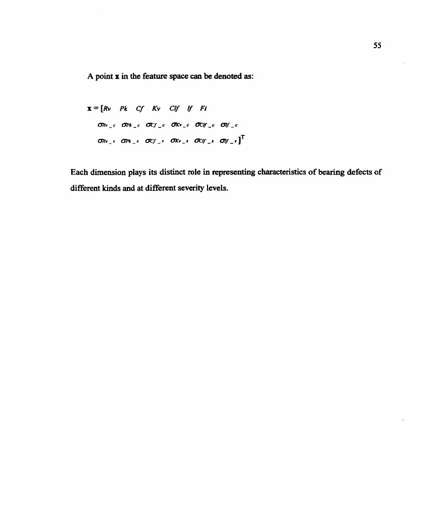
A point x in the feature space can be denoted as:
Each dimension piays its distinct role in representing characteristics of bearing defects of
different kinds and at different severity levels.
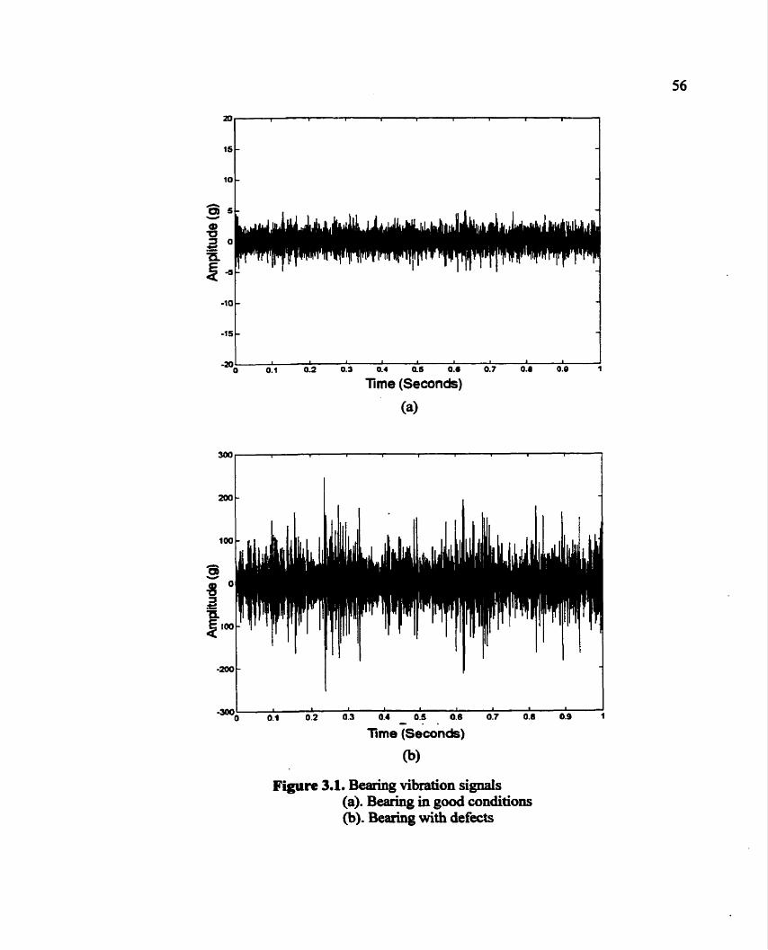
-200 -
-=o 6, o; 03 o i - . . 0:s 0's 67 oh 04 1
Ttme (Seconds)
(b)
-10
-15
Figure 3.1. Bearing vibration signals (a). Bearing in good conditions (b). Bearing with defects
- -
- -
6 0 0:2 Of3 0:4 0k 0:. 0:7 0:. OIO 1
Time (Seconds)
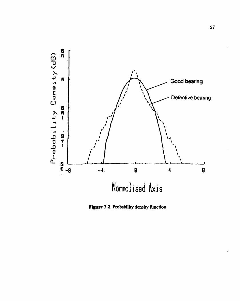
Figure 3.2. Probability density fhction
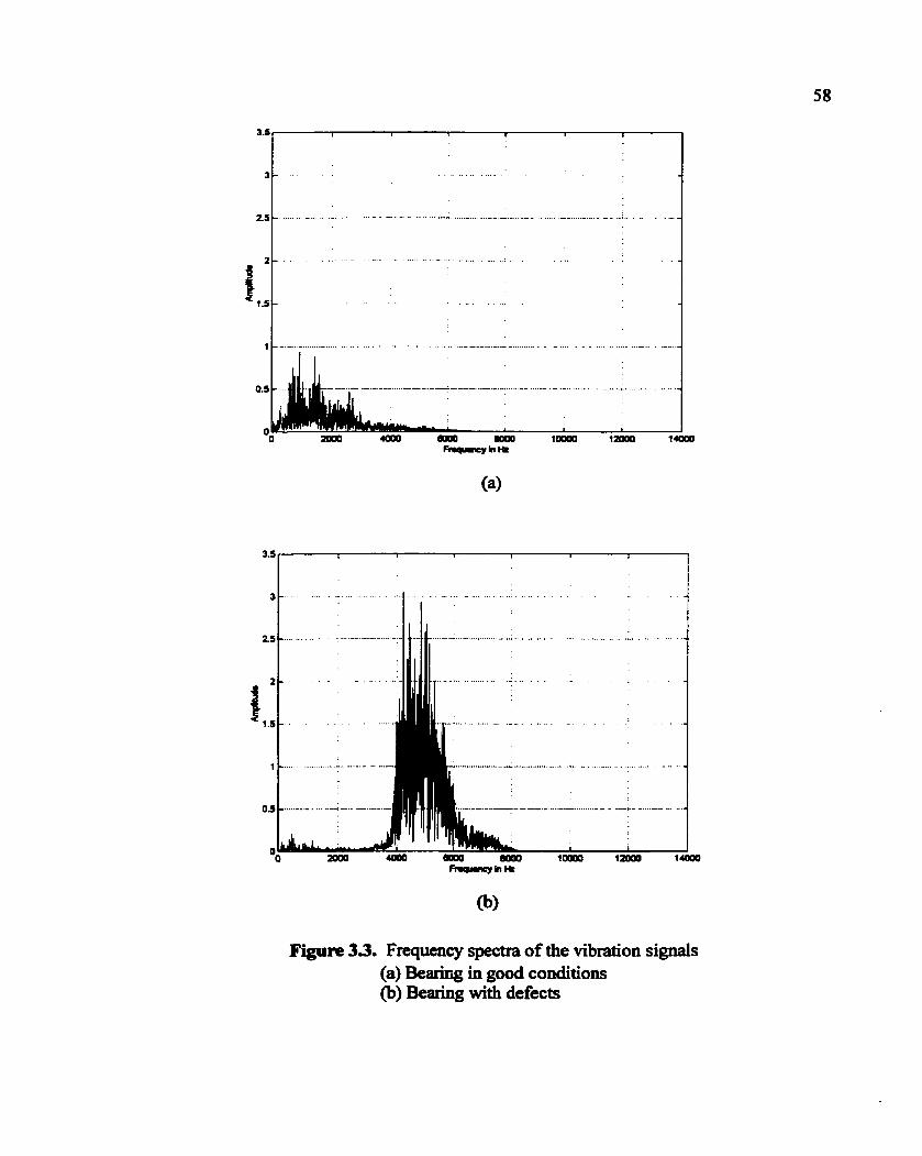
Figure 33. Frequency spectra of the vibration signals (a) Bearkg in good conditions (b) Bearing with defects
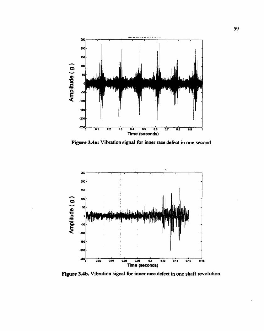
0:4 d2 o 0 5 0 0:7 8 04 ! Time (seconds)
Figure 3.4.: Vibration signal for inner race defect in one second
0 . h 0.b A;# 0.k 0:l 0.12 0 .4 0 . ; ~ 0.!8
Time (seconds)
Figure 3.4b. Vibration signal for inner race defect in one shaft revolution
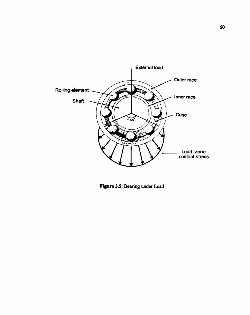
Rolling element
Shaft
Figure 3.5: Bearing under Load
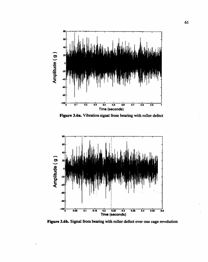
-1001 1 I I P 1 I I I I I
0 0.1 0.2 0.3 0.4 0.5 0-6 0.7 0.8 0.9 1
Time (seconds)
Figure 3.6a. Vibration signal fiom bearing with roller defect
0.k 0:1 0 0'2 ah 0:3 0.k 0; 0.b O!S
Time (seconds)
Figure 3.6b. Signal from bearing with roller defect over one cage revolution
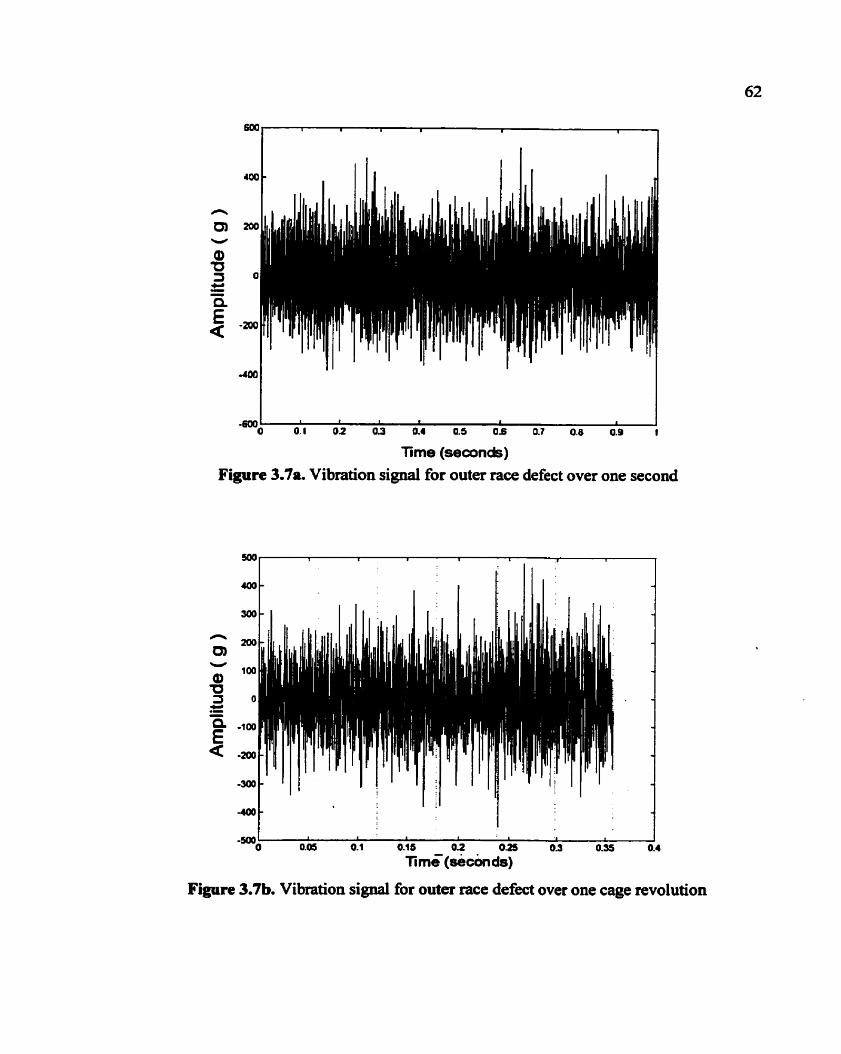
Time (seconds)
Figure 3.7a. Vibration signal for outer race defect over one second
Figure 3.7b. Vibration signal for outer race defect over one cage revolution
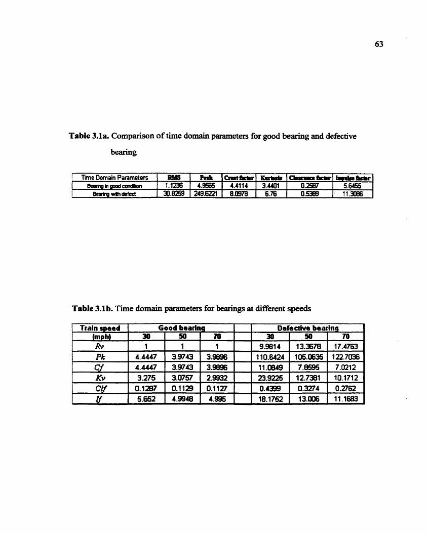
Table 3.la. Comparison of time domain parameters for good bearing and defective
bearing
Table 3.lb. Time domain parameters for bearings at different speeds
t Time Domain Parameten : Bmhginpood#ndbn 1
i ~ c a i n p w t h ~ f e
RJYIS 1.1236 Jl.8259
! Train meed i (mph)
Rv i f Pk
Cf Kv
Peak 4 . S
249.6221
Defective bearing
Clf
Good beating 70
17.4763 122.7036 7.0212 10.1712
30 9.9814
1 10.6424 11.0869 M.9225
'kbr 5.6455
. 11.3086
C l s r t W 4.4114 8.0978
70 1
3.9096 3.- 2.9932
30 1
4.447 4.447 3.275
SO 13378 105.0635 7.- 12.7381
50 7
1 3.9743 3.9743 3.0757
K u W s 3.4401 6.76
0.1127 4.995
0.1287 5.652
CbmmsWr 0.2W 0.5389
0.1129 4.9948
0.2762 11.1683
0.4399 18.1752
0.3274 13.006
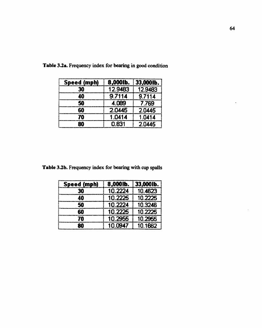
Table 3.2a. Frequency index for bearing in good condition
Table 32b. Frequency index for bearing with cup spalls
Table 33a. Time domain parametem of six segments for bearing with inner race defect
Table 33b. Segmentation parameters (shaft fkquency) for bearing with Inner race defect
! Time Domain I Parametem
fi I
: Pk cf a
Kv Clf
:
; If -
- ..... Segment Index
f Segmentation I ~ a r a r n e t . ~ a 08.J r i QM, s
t W - 3 i- 1 m-r : W -3
W-J
1 7.8491 22.9907 2.9301 3.4406 6 . s 3.7442
Train Running Speed (mph)
2 4.9825 12.5721 2.5233 3.1313 5.6337 3.2916
30 8.8932 38.2407 1.2548 4.991 3 3.3334 2.3333
3 6.0294 15.125 2 . 2.5077 5.31 18 3.1451
40 11.8269 38.!5805 0.7543 1 7959 2.381 1 1 264
4 10.3168 31.183 3.0225 3.5191 6.9424 3.9892
80 80.5279 168.7093 0.4965 1.5312 4.1686 0.945
SO 43.3719 154.0913 0.6159 1.1 19 1.9795 0.7626
5 20.9734 82.7235 3.9442 6.0414 10.7427 5.8321
6 29.7816 106.134 3.5637 5.7815 8.4341 4.8886
60 50.9753 173.0131 0.7551 2.4848
. 4.3528 1 -4364
70 95.7304 156.1674 0.6564 1 -6738 4.2932 1 -2240
Table 3.4.. Time domain parameters of six segments for bearing in good condition
Tabk 3Ab. Segmentation parameters (sh& frequency) for bearing in good condition
f Time Domain i Parameters i ; Av 2
i Pk Cj Kv
I CU i
Segment Index a
j Seqmentation Parameten
m-J t-
m-3 L
a C l - 3 B
i m-3
i W -1 b ? : W-1
1 1.2348 3.8438 3.1129 3.6318 7.814 4.24
Train Running Speed (mph) -
2 0.8953 2.6677 2.9797 3.2602 6.7993 3.8483
30 0.0815 0.4533 0.394 0.3326 0.298 0.5025
3 0.9193 2.8486 3.0967 3.4334 7.258
4 . m
40 0.1 129 0.4612 0.2658 0 . W 0.3335 0.397
4 1.069
3.5156 3.2887 3.4150 8.5502 4.5622 -
60 0.3689 1.0771 0.2522 0.31 56 0.3268 0 . m
50 0.1845 0.3457 0.3022 0.2864 0.5872 0.4742
5 1.4095 3.2048 2.9832 3.5043 7.0656 3.9461
70 0.1698 1 .0661 0.253 0.3481 0.S4 0 . B
6 1.1504 3.1873 2.7705 3.0433 6.2527 3.5487
80 0.3229 1 -3224 0.1507 0.2309 0.4343 0.2342
Table 3.5a. Time domain parameters of six segments for bearing with roller defect
Table 3e5bm Segmentation parameters (cage fkquency) for bearing with roller defect
i Time Domain f Parametem i & f
pk i Cf I Kv I Clf
Segment Index
:
I Segmentation f i Parameten i a& -c
f m - 6
f : ..... W - 6
-6
i m - 6
i W - 6 .
1 15.4603 52.7938 3.4148 3.4407 2.5953 4 . 4 s
Train Running Speed (mphl
2 21.138 80.3135 3.7995, 3.5667 2.8607 4.8963
30 2.5264 12.813 0.31 01 0.2841 0.2729 0.438
70 4.148
13.0024 0.129 0.1679 0.3152 0.206
3 20.0997 67.957 3.381 3.297 2.5248 4.3404
80 4.6758 12.7737 0.2257 0.3624 0.65~2 0.3535
4 16.884
58-8185 3.4837 3.2428 2.5376 4.4146
5 18.1045 !54.9398 3.0346 3.076 2.2125 3.8412
60 3.1617 8.9394
40 1.7198 6.6802
6 14.7843 43.6795 2.9544 2.7636 2.1091 3.6936
50 1.8943 0.0384
0.2983 0.1 24
0.2921 0.3784
0.2534 0.2015 0.3684 0.3553
0.1 129 0 2299 0.286 0.194
Table 3.6a. Time domain parameters of six segments for bearing with outer race defect
, Time Domain f Parametem
Rv Pk
I I Cf I Kv I
i Cr r f
Table 3.6b. Segmentation parameters (cage frequency) for bearing with outer race defect
i f Segmentation j Parameten i m~ -6 I
--6 I i t W-6
i i - -c i QCEl-c i i : W -6
Segment Indew 1
86.5941 Z.2959
2.7288 3.- 2.6387 3.4454
Train Running Speed {mph)
2 88-7159 249.6868 2.8145 2-5748 2.5762 3.428
80 17.21 57
70 41 . a 1
30 6.4294
3 93.7776
276.2982 2.9463 3.1394 2.6562 3.7322
22.7424 0.1 149 0.2668 0.1 152 0.1843
40 3.6!519
4 92.0558
201.2072 3.0547 3.2082 2.9412 3.8514
1 12.3491 0.1529 0.1761 0.391 3 0.2366
22.9486 0.2786 0.5665 0.3587 0.4306
50 8.7423
37.4694 0.1 232 0.1 546 0.3358 0.195
5 105.5642 270.3251 2.5608 2.5432 2.4246 3.1616
60 14.5054
6 103-6473 282.8041 2.7285 2.8146 2.6287 3.4277
76.61 23 0.3423 0.4154 0.5006 0.4872
44.1 272 0.1275 0.1734 0.21 73 O.lf38
CHAPTER FOUR:
NEURAL NETWORKS FOR NONLINEAR MAPPING
4.1 Introduction
After constructing the feature space, we propose to map the data £?om the 19-
dimensional feature space to a 2-dimensional classification space since an image in a 2D
space can be easily visualized and analyzed by a human observer, which greatly assists
the design of an effective pattern classifier.
In the earlier work [Sun, et al., 19981, linear mapping was performed to project
samples in the feature space to the classification space. In other words, elements in the
classification space are assumed a weighted linear combination of those in the feature
space. The weights are determined through the data sets with known bearing conditions.
The least squared criterion is used to create cluster effects on data belonged to the same
class. However, the linear mapping, although simple in computation, does not necessarily
guarantee that classes are sepmtable by linear boundaries in the classification space.
Pattern belonging to different classes may overlap in the classification space. The results
suggest that a nonlinear mapping between the two spaces may be desirable.
In this research, a three-layered artificial neural network is introduced to accomplish
the nonlinear mapping fiom the feature space to the classification space. Three-layered
networks are sufficient for representing the non-linear relations between the input and
output and they have relatively simple architecture. One advantage of the artificial neural
network approach is that it allows us to construct complicated non-linear relations
between input and output when deficient analytical description is available. Although
neural networks are computationally intensive, most of the intense computation takes
place during the training process which can be conducted off-line. Once the network is
70
trained for a particular task, operation is relatively fast and unknown samples can be
rapidly identified in the field. They have the ability to recognize relations between the two
sets of data even when the information comprising these data is noisy or incomplete.
[Alguindigue, et al., 1 993; Unal, 1 994; Subrahmanyam, et al., 1 9971.
Assume a total number of N samples are used for training. Each sample belongs to
one class of a total of K classes with K cluster centers uh k = 1, . . . , K. The nonlinear
mapping between two spaces can be expressed as:
where X E R ' ~ is a vector in the feature space denoted as [RW pk C/ KV cr/ ~f ~i OR" -=
mk - C o ty -c m y - = tzy-c b ~ v - , UP^ -.r QT.J-+ b ~ v - . ~ m : ~ -.r bl/ -.r lT, while
y ~ ~ 2 represents a vector containing the corresponding coordinates in the classification
space denoted as [r, When artificial neural networks are to be trained to learn the
non-linear relations, known values of x and y are used as input and output respectively.
The purpose of mapping between the feature and classification space is for dimension
reduction while creating the best clustering effect for the N samples belonging to the
same class around their own specified cluster center u'. Successful mapping allows
application of the simple piecewise linear boundaries that will be discussed in chapter 5.
4.2 Artificial Neural Networks
Artificial Neural networks (ANN) can be implemented as computer algorithms that
can be used to describe a system in terms of relations between input and output. They
represent an alternative method of describing systems when it is very difEcult or
impossible to use analytical approaches. They have been used in a wide variety of
applications related to manufacturing. These applications include process control, quality
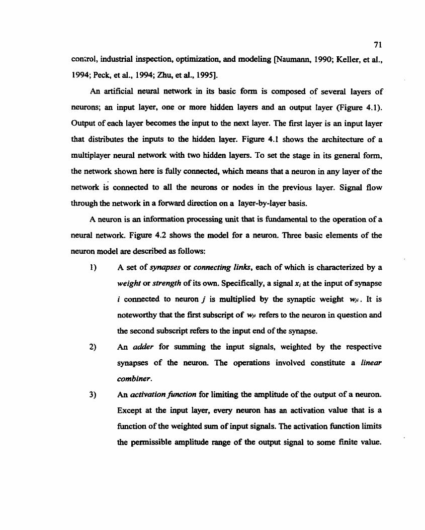
71
con~ol, industrial inspection, optimization, and modeling [Naumann, 1990; Keller, et al.,
1994; Peck, et ai., 1 994; Zhu, et al., 19951.
An artificial neural network in its basic form is composed of several layers of
neurons; an input layer, one or more hidden layers and an output layer (Figure 4.1).
Output of each layer becomes the input to the next layer. The first layer is an input layer
that distributes the inputs to the hidden layer. Figure 4.1 shows the architecture of a
multiplayer neural network with two hidden layers. To set the stage in its general form,
the network shown here is fully connected, which means that a neuron in any layer of the
network is connected to all the neurons or nodes in the previous layer. Signal flow
through the network in a forward direction on a layer-by-layer basis.
A neuron is an information processing unit that is fundamental to the operation of a
neural network. Figure 4.2 shows the model for a neuron. Three basic elements of the
neuron model are described as follows:
1 ) A set of synapses or connecting links, each of which is characterized by a
weight or strength of its own. Specifically, a signal xi at the input of synapse
i connected to neuron j is multiplied by the synaptic weight wji. It is
noteworthy that the first subscript of wji refers to the neuron in question and
the second subscript refers to the input end of the synapse.
2) An adder for summing the input signals, weighted by the respective
synapses of the neuron. The operations involved constitute a linear
combiner.
3 An octivationfinction for limiting the amplitude of the output of a neuron.
Except at the input layer, every neuron has an activation value that is a
function of the weighted sum of input signals. The activation function limits
the permissible amplitude range of the output signal to some finite value.
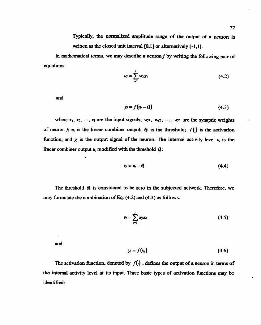
Typically, the normalized amplitude range of the output of a neuron is
written as the closed unit interval [O, 1 ] or alternatively [- 1,1].
In mathematical terms, we may describe a neuron j by writing the following pair of
equations: I
and
where XI, x2 , . . ., XI are the input signals; w,~. wjz, . . ., W ~ I are the synaptic weights
of neuron j; u, is the linear combiner output; 6) is the threshold; f (-) is the activation
hction; and y, is the output signal of the neuron. The internal activity level v, is the
linear combiner output u, modified with the threshold 6) :
vj = uj - 6)
The threshold t?J is considered to be zero in the subjected network. Therefore, we
may formulate the combination of Eq. (4.2) and (4.3) as follows:
I-I
and s = f (w)
The activation hction, denoted by f () , defines the output of a neuron in terms of
the internal activity level at its input. Three basic types of activation functions may be
identified:
73
1) Threshold Function
In this model, the output of a neuron takes on the value of 1 if the total internal
activity is nonnegative and 0 otherwise.
2) Piecewise-Linear Function
This form of activation function may be viewed as an approximation to a non-linear
amplifier. The amplification faftor inside the linear region of operation is assumed to be
unity.
3) Sigmoid Function
The sigmoid function is by far the most common form of activation function used in
the construction of neural networks. It is defined as a strictly &creasing function that
exhibits smoothness and asymptotic properties. An example of the sigmoid is the Logistic
function, defined by
A sigmoid function assumes a continuous range of values &om 0 to 1 or -1 to 1 and
is differentiable as shown in Figure 4.3.
4.2.1 Multilayer Fe&orward Artifkial Neural Network
Multilayer feedforward artificial neural networks have been widely adopted for
many ANN applications. They have been applied successfidly to solve complicated
problems by training them in a supervised manner with the popular algorithm known as
the error back-propagation algorithm maykin, 19941. The basic idea of back-propagation
was first described by Werbos in his Ph.D. thesis [Werbos, 19741, in the context of
general networks with neural networks representing a special case. The development of
the back-propagation algorithm represents a "landmark" in neural networks in that it
74
provides a computationally efficient method for the training of multiplayer perceptrom.
The trained network based on the error back-propagation algorithm often produces
surprising results in applications where explicit derivation of input-output relationship is
almost impossible.
Training of feedforward neural networks takes place in an iterative fashion. Each
iteration cycle involves a forward-propagation pass followed by an error backward-
propagation pass to update the connection weights. Figure 4.4 depicts a portion of the
multiplayer neural network with the two passes.
The forward-propagation pass starts when the input nodes receive their activation
levels in the form of an input pattern. Then, forward-propagation proceeds through the
hidden layers up to the output layer by computing the activation levels of the nodes in
those layers. Finally, a set of outputs is produced as the actual response of the network.
During the forward pass the synaptic weights of the network are all fixed.
Weight adjustment is accomplished by propagating the error function of the output
back through the net and modifying all the weights. The iterative method propagates error
hc t ion required to adapt weights back &om nodes in the output layer to nodes in the
hidden layers in accordance with the training rule. The weights are adjusted so as to make
the actual response of the network move closer to the desired response.
Training sets are repeatedly presented and weights modified until the error between
the predicted and actual output is less than a specified value (error criterion). Once the
neural network has been trained in this way, it should be possible to relate input patterns
with the appropriate output patterns [Chiou, et al., 1992). To use the trained ANN, a new
input set is simply presented to the network and the network calculates an output solution.
Properly-trained ANNs are able to give reasonable answers when presented with inputs
that they have never seen. Typically, a new input will lead to an output with similar
features to the comct output for input vectors with similar features used in training.
75
Therefore, it is possible to train a neural network on a representative set of input/target
pairs and get good results without training it on alf possible input/output pairs.
4.2.2 Error Back-Propagation Training Algorithm
Before the network could be used for the non-linear transforming purposes in this
work, we decide to apply the supervised learning technique to train the neural network
using a set of known inputs and corresponding outputs.
Inputs are the features extracted from bearing vibration signals with known bearing
conditions. Desired outputs are the cluster centers arbitrarily chosen for each class.
Assume there are total K classes, K cluster centers u,, k = 1, . . ., K, are chosen in the first
quadrant of a 2D coordinate h e in order to locate the desired output associated with
each of the K classes. Although their arrangement is somewhat arbitrary, we placed them
evenly on a unit circle in the first quadrant of a 2D space. Non-linear mapping is applied
to cluster the entire samples belonged to the same category in the feature space around
their own specified cluster center ar in the classification space.
Consider a three-layered ANN with only one hidden layer as shown in Figure 4.5. In
the figure, index i refers to nodes at the input layer, index j ~ f e r s to nodes at the hidden
layer, and index k refers to nodes at the output layer. widenotes the weight of the
connection between node i in the input layer and j in the hidden layer, while v~denotes
the weight of the connection between node j in the hidden layer and k in the output layer.
Assume xi, i = 1, . . ., I, are input signals, a neuron j in the hidden layer can be described by
writing the following pair of equations:
and
where 6, represents the internal activity level of the neuron j, y, is the output of the neuron
j and f () is the activation hmction of the hidden layer.
Similarly, a neuron k in the output layer can be described by writing the following
pair of equations:
and
where c, represents the internal activity level of the neuron k, or is the output of the
neuron k and fc) is the activation hc t ion of the output layer which is assumed to be the
same as the hidden layer.
Let p be the index representing the training set and P the total number of samples
involved in training the network. At any iteration, the sum of squared errors for the pth
training sample between the target and actual output is defined as:
Where:
K is the number of output nodes of the network.
O k d represents the target output at node k.
0, is the actual output at node k.
The average squared error Em among all the training sets can be calculated as
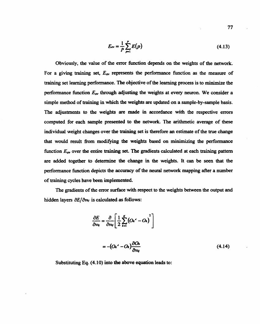
Obviously, the value of the error fiulction depends on the weights of the network.
For a giving training set, Em represents the performance function as the measure of
training set learning performance. The objective of the learning process is to minimize the
performance function Em through adjusting the weights at every neuron. We consider a
simple method of tmhing in which the weights are updated on a sample-by-sample basis.
The adjustments to the weights are made in accordance with the respective errors
computed for each sample presented to the network. The arithmetic average of these
individual weight changes over the training set is therefore an estimate of the true change
that would result from modifying the weights based on minimizing the performance
function E, over the entire training set. The gradients calculated at each training pattern
are added together to determine the change in the weights. It can be seen that the
performance function depicts the accuracy of the neural network mapping after a number
of training cycles have been implemented.
The gradients of the error surface with respect to the weights between the output and
hidden layers d E / h h is calculated as follows:
Substituting Eq. (4.10) into the above equation leads to:
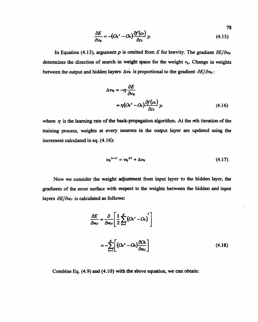
In Equation (4.13), argument p is omitted from E for brevity. The gradient aE/&k,
determines the direction of search in weight space for the weight v,. Change in weights
between the output and hidden layers Avk is proportional to the gradient aE/&& :
where 7 is the Leaming rate of the back-propagation algorithm. At the nth iteration of the
training process, weights at every neurons in the output layer are updated using the
increment calculated in eq. (4.16):
Now we consider the weight adjustment from input Layer to the hidden layer, the
gradients of the error surface with respect to the weights between the hidden and input
layers dE/aWji is calculated as follows:
Combine Eq. (4.9) and (4.10) with the above equation., we can obtain:
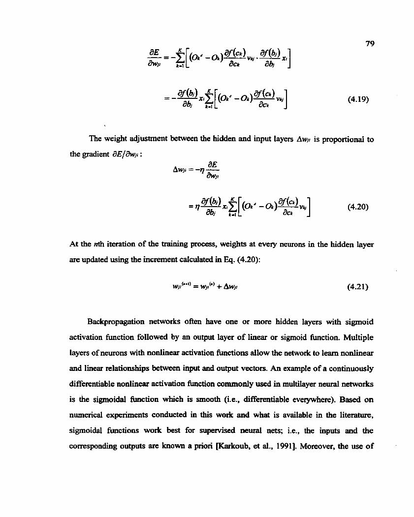
The weight adjustment between the hidden and input layers Aw,~ is proportional to
the gradient dE/&vji :
At the nth iteration of the training process, weights at every neurons in the hidden layer
are updated using the increment calculated in Eq. (4.20):
Backpropagation networks often have one or more hidden layers with sigmoid
activation fimction followed by an output layer of linear or sigmoid bction. Multiple
layers of neurons with nonlinear activation fbctions allow the network to learn nonlinear
and linear relationships between input and output vectors. An example of a continuously
differentiable nonlinear activation hct ion commonly used in multilayer neural networks
is the sigrnoidal function which is smooth (i.e., differentiable everywhere). Based on
numerical experiments conducted in this work and what is available in the literature,
sigmoidal functions work best for supervised neural nets; i.e., the inputs and the
corresponding outputs are known a priori [Karkoub, et al., 19911. Moreover, the use of
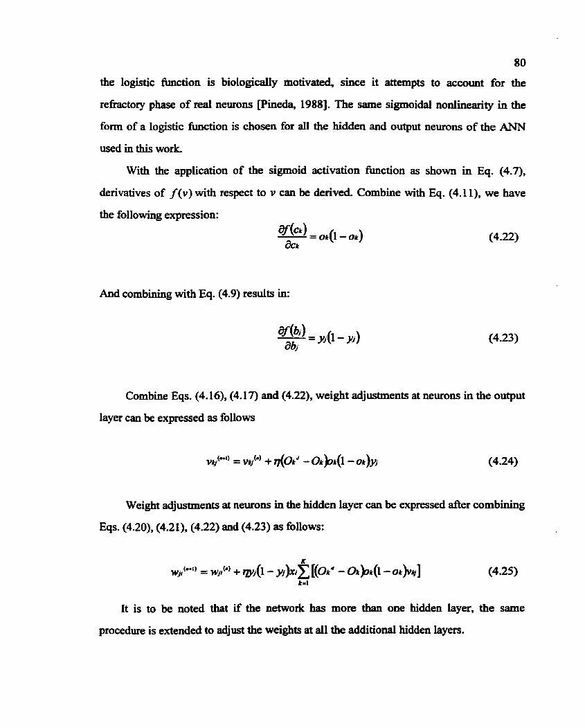
80
the logistic hc t ion is biologically motivated, since it attempts to account for the
refkctory phase of real neurons pineda, 1988 3. The same sigrnoidal nonlinearity in the
form of a Logistic hc t ion is chosen for all the hidden and output neurons of the ANN
used in this work.
With the application of the sigmoid activation hc t ion as shown in Eq. (4.7),
derivatives of f (v) with respect to v can be derived. Combine with Eq. (4.1 I), we have
the following expression:
And combining with Eq. (4.9) results in:
Combine Eqs. (4.16), (4.1 7) and (4.22), weight adjustments at neurons in the output
layer can be expressed as follows
Weight adjustments at neurons in the hidden layer can be expressed after combining
Eqs. (4.20), (4.21), (4.22) and (4.23) as follows:
It is to be noted that if the network has more than one hidden layer, the same
procedure is extended to adjust the weights at all the additional hidden layers.
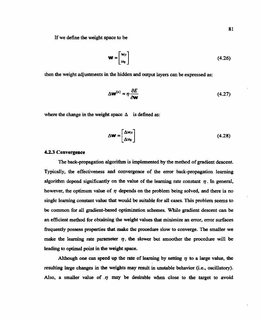
If we define the weight space to be
then the weight adjustments in the hidden and output layers can be expressed as:
where the change in the weight space A is defined as:
4 2 3 Convergence
The back-propagation algorithm is implemented by the method of gradient descent.
Typically, the effectiveness and convergence of the error back-propagation learning
algorithm depend significantly on the value of the learning rate constant q . In general,
however, the optimum value of 7 depends on the problem being solved, and there is no
single learning constant value that would be suitable for all cases. This problem seems to
be common for all gradient-based optbization schemes. While gradient descent can be
an efficient method for obtaining the weight values that minimize an error, error surfaces
frpquently possess properties that make the procedure slow to converge. The smaller we
make the learning rate parameter q , the slower but smoother the procedure will be
leading to optimal point in the weight space.
Although one can speed up the rate of learning by setting q to a large value, the
resulting large changes in the weights may result in unstable behavior (i.e., oscillatory).
Also, a smaller value of .q may be desirable when close to the target to avoid
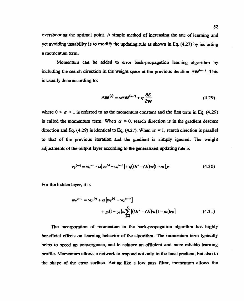
82
overshooting the optimal point. A simple method of increasing the rate of learning and
yet avoiding instability is to modify the updating rule as shown in Eq. (4.27) by including
a momentum tenn.
Momentum can be added to error back-propagation learning algorithm by
including the search direction in the weight space at the previous iteration AW(~-'). This
is usually done according to:
where 0 < a < 1 is referred to as the momentum constant and the first term in Eq. (4.29)
is called the momentum term. When a = 0, search direction is in the gradient descent
direction and Eq. (4.29) is identical to Eq. (4.27). When a = 1, search direction is pamllel
to that of the previous iteration and the gradient is simply ignored. The weight
adjustments of the output layer according to the generalized updating rule is
For the hidden layer, it is
The incorporation of momentum in the back-propagation algorithm has highly
beneficial effects on learning behavior of the algorithm. The momentum term typically
helps to speed up convergence, and to achieve an efficient and more reliable learning
profile. Momentum allows a network to respond not only to the local gradient, but also to
the shape of the error d a c e . Acting like a low pass filter, momentum allows the
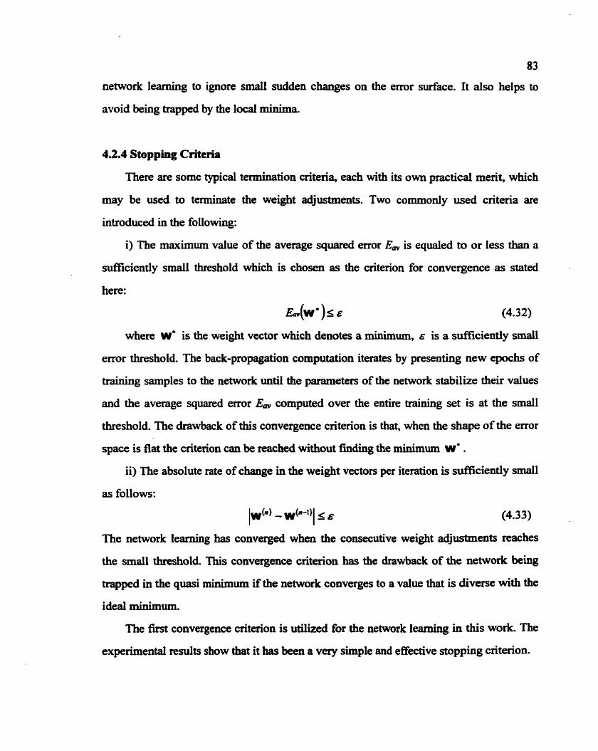
83
network learning to ignore small sudden changes on the error surface. It also helps to
avoid being trapped by the local minima.
4.2.4 Stopping Criteria
There are some typical termination criteria, each with its own practical merit, which
may be used to terminate the weight adjustments. Two commonly used criteria are
introduced in the following:
i) The maximum value of the average squared error Em is equaled to or less than a
sufficiently small threshold which is chosen as the criterion for convergence as stated
here:
E - w ' ) ~ E (4.32)
where W' is the weight vector which denotes a minimum, E is a sufficiently small
error threshold. The back-propagation computation iterates by presenting new epochs of
training samples to the network until the parameters of the network stabilize their values
and the average squared error Em computed over the entire training set is at the small
threshold. The drawback of this convergence criterion is that, when the shape of the error
space is flat the criterion can be reached without finding the minimum W' . ii) The absolute rate of change in the weight vectors per iteration is sufficiently small
as follows:
IwC) - ,,,,b-') 1 6 I (4.33)
The network learning has converged when the consecutive weight adjustments reaches
the small threshold. This convergence criterion has the drawback of the network being
trapped in the quasi minimum if the network converges to a value that is diverse with the
ideal minimum.
The first convergence criterion is utilized for the network learning in this work. The
experimental results show that it has been a very simple and effective stopping criterion.
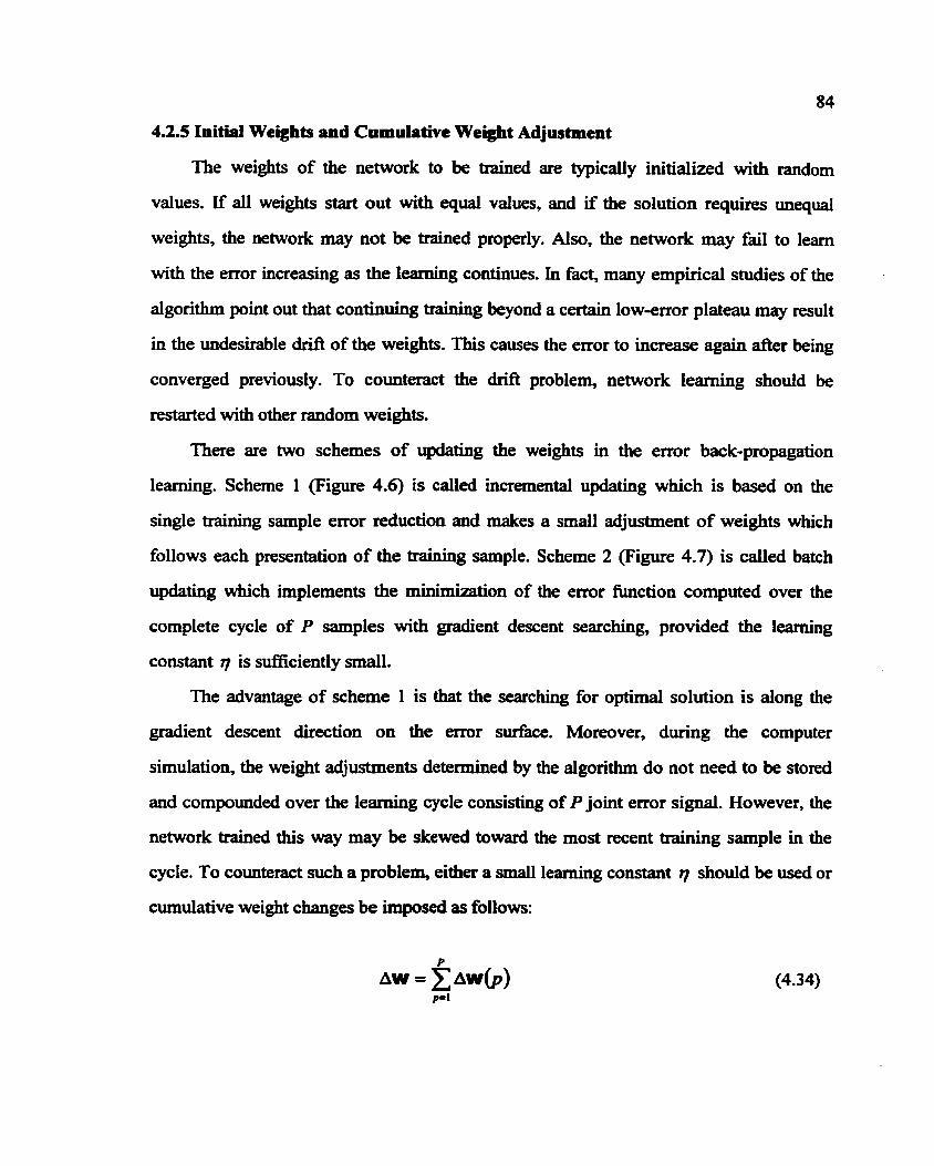
4.2.5 Initial Weights and Cumulative Weight Adjustment
The weights of the network to be trained are typically initialized with random
values. If all weights start out with equal values, and if the solution requires unequal
weights, the network may not be trained properly. Also, the network may fail to learn
with the error increasing as the leaning continues. In fact, many empirical studies of the
algorithm point out that continuing training beyond a certain low-error plateau may result
in the undesirable drift of the weights. This causes the error to increase again afker being
converged previously. To counteract the drift problem, network learning should be
restarted with other random weights.
There are two schemes of updating the weights in the error back-propagation
learning. Scheme 1 (Figure 4.6) is called incremental updating which is based on the
single training sample error reduction and makes a small adjustment of weights which
follows each presentation of the training sample. Scheme 2 (Figure 4.7) is called batch
updating which implements the minhbt ion of the error fhction computed over the
complete cycle of P samples with gradient descent searching, provided the learning
constant q is sufficiently small.
The advantage of scheme 1 is that the searching for optimal solution is along the
gradient descent direction on the error surface. Moreover, during the computer
simulation, the weight adjustments determined by the algorithm do not need to be stored
and compounded over the learning cycle consisting of P joint error signal. However, the
network trained this way may be skewed toward the most recent training sample in the
cycle. To counteract such a problem, either a small learning constant 7 should be used or
cumulative weight changes be imposed as follows:
85
for both output and hidden layers, where A W ( ~ ) represents the change in the weight
space for the pth training pattern. The weight adjustment in this scheme is implemented at
the conclusion of the complete learning cycle. It takes the average effects of all the
training cycles. Provided that the learning rate is small enough, the cumulative weight
adjustment can still implement the algorithm close to the w e n t descent minhkation.
Although both scheme 1 and scheme 2 can bring satisfactory solutions, attention
should be paid to the fact that the training works the best under random conditions. It
would thus seem advisable to use the incremental weight updating after each pattern
presentation, but choose patterns in a random sequence. This introduces much-needed
noise into the training and alleviates the problems of averaging and skewed weights
which would tend to favor the most recent training patterns.
4.3 Experimental Determination of Optimal Neural Network
4 e 3 e 1 e Network Architecturm with Optimal Hidden Layer
The multilayered ANN trained with the back-propagation algorithm is applied to
perform the nonlinear input-output mapping. One of the most important attributes of a
multilayered neural network design is choosing the architecture. The number of input
nodes is simply determined by the dimension of the input vector.
In this thesis, the input-output relationship of the network defines a mapping from a
19-dimensional feature space to a Zaimensional classification space. Thus, the number of
input nodes is chosen to be nineteen and the number of neurons in the output layer is two.
This inputoutput mapping is assumed to be infinitely continuously differentiable. In
assessing the capability of the neural network, two fundamental questions arise:
I ) Determine the number of hidden layers:
It was Cybenko who demonstrated rigorously for the first time that a single hidden
layer is suilicient to uniformly approximate any continuous h c t i o n with support in a
86
unit hypercube [Cybenko, 19881. He introduced the universal approximation theorem
which states that a single hidden layer is d c i e n t for a multilayered neural network to
compute a uniform approximation to a giving training set represented by the set of inputs
and a desired (target) output. A single hidden layer is chosen for the ANN used in this
work.
2) Determine the size of the hiden layer:
Size of each hidden layer is mostly determined through trial and error process
depending on individual problems. The exact analysis of the issue is rather difFcult
because of the complexity of the network mapping and due to the non-deterministic
nature of the training procedures. If there are too few nodes the neural network will fail to
memorize the training process and lead to underfitting. Too many neurons can contribute
to overfitting, in which all training points are well fit, but the fitting curve takes wild
oscillations between these points. Based on trial and error, the size of 24 is found to be
the optimal compromise between underfitting and overfitting with faster convergence
compared to 20 and 26 hidden nodes (see Table 4.1). Therefore, the finally obtained
optimal architecture of the network is 19-24-2 as shown in Figure 4.8. It is shown that the
input layer has 19 nodes, each of which represents a parameter in the feature space
denotedas as [h fk Cf Kv Clf If Fi ~ ~ v - e a r k - c CRY-= m - c b t : l j - c mf-= ORV - s
m - . gty -I bkv - .* mu -.T my - S lr. The output layer has two neurons, each of which
contains a coordinate value in the 2D space denoted as 1% y.lT.
4.3.2. Accelerated Convergence through Learning-Rate Adaptation
Situation arises when a constant learning rate q does not produce satisfactory
performance. For example, on a flat e m r surface, too many steps may be required to
compensate for the small gradient value. In this work we use a heuristic technique to
87
determine the variable learning rate in order to accelerate the convergence of bck-
propagation learning. Four heuristics are considered as guidelines maykin, 19941 :
Heuristic 1. Every adjustable network parameter should have its own adjustable
learning-rate parameter. The back-propagation algorithm may be slow to converge
because of a fixed learning rate that may not suit a l l portions of the error suxface. In other
words, a learninggrate parameter appropriate for the adjustment of one weight is not
necessarily appropriate for the adjustment of other weights in the network. This method
recognizes this fact by assigning a different learning-rate parameter to each adjustable
weight @ m e t e r ) in the network.
Heuristic 2. Every learning-rate parameter should be allowed to vary fmm one
iteration to the next. Typically, the error surface behaves differently in different regions
and different dimensions. In order to match this variation, heuristic 2 allows the learning
rate to vary from iteration to iteration.
Heuristic 3. When the derivative of the performance fimction with respect to a
weight has the same algebraic sign for several consecutive iterations, the learning-rate
parameter for that particular weight should be increased. The current operating point in
the weight space may lie on a relatively flat portion of the error surface along a particular
weight dimension. This results in the derivative of the performance function with respect
to that weight with the same algebraic sign, that is, the same gradient direction, for
several consecutive iterations. Heuristic 3 states that in such a situation the number of
iterations required to move across the flat portion of the error surface may be reduced by
increasing the learning-rate parameter appropriately.
Heuristic 4. When a E / h n alternates for several consecutive iterations of the
algorithm, the learning-rate parameter for that weight should be decreased. This is the
opposite situation to the above. When the current operating point in weight space lies on a
portion of the error surface along a weight dimension of interest that exhibits peaks and
88
valleys (i.e., the surface is highly curved), then it is possible for the derivative of the
performance h c t i o n with respect to that weight to change its algebraic sign from one
iteration to the next. In order to prevent the weight adjustment from oscillating, the
learning-rate parameter for that particular weight should be decreased appropriately.
It should be noted that the use of a non-uniform and time-varying learning rate
modities the back-propagation algorithm significantly. Specifically, the modified
algorithm no longer performs a gradient descent search. Rather, the adjustments applied
to the weights are based on (1) the partial derivatives of the error surface with respect to
the weights, and (2) estimates of the curvatures of the error surface at the current
operating point in weight space along the various weight dimensions.
Let t l (n) denote the learning rate assigned to the weight at iteration n for both
hidden and output layers. The learning-rate update rule is defined as follows:
where 0 < y < 1 is a positive constant called the control step-size parameter for the
leaming rate adaptation procedure. The partial derivatives d ~ ' " ' / d r . r ( " ) and
E ~ ' / . " ' refer to the derivative of the error surface with respect to the weight
w./" at iterations n and n-1 respectively. It can be observed that when the partial
derivative has the same algebraic sign on two consecutive iterations, the adaptation
procedure increases the learning rate for the weight W.V. Correspondingly, the learning
along that direction will be fast. When the derivative alternates on two consecutive
iterations, the adaptation procedure decreases the leaming rate for the weight W.V.
Consequently, the learning along that direction will be slow.
Many parameters of the network can be adjusted during training to provide optimal
performance. Unfortunately, a systematic method for selection of the most appropriate
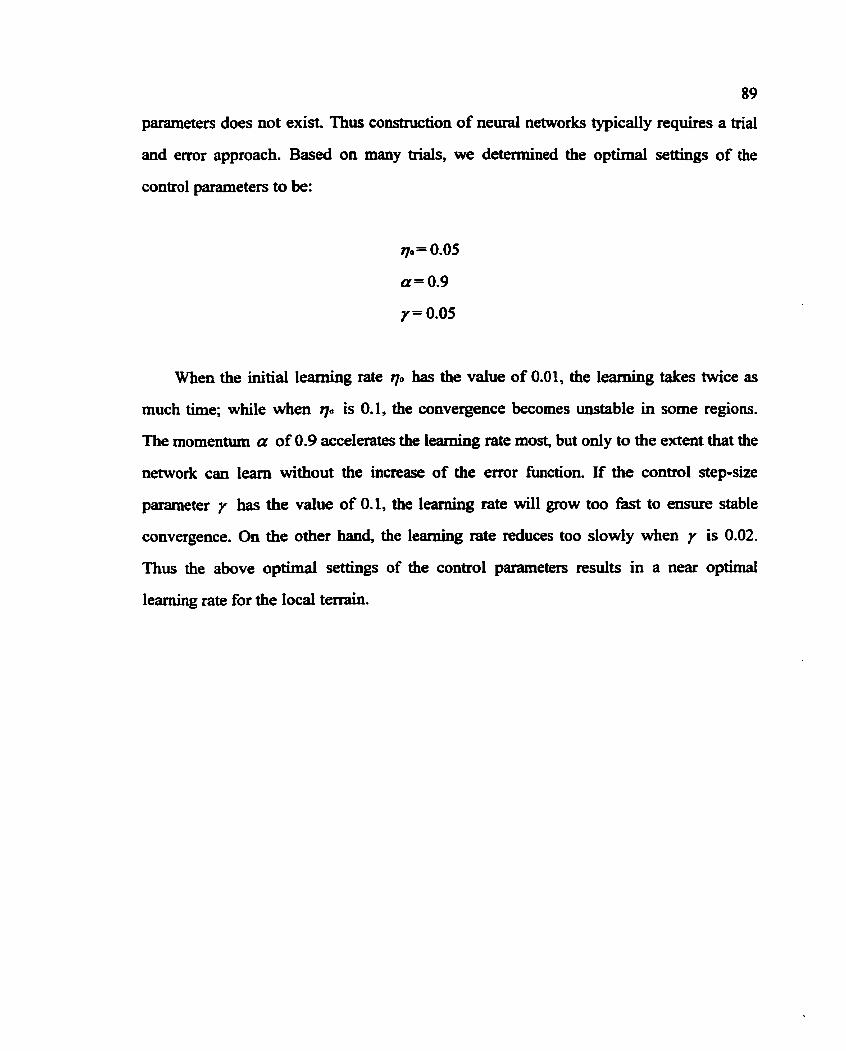
89
parameters does not exist. Thus construction of neural networks typically requires a trial
and error approach. Based on many trials, we determined the optimal settings of the
control parameters to be:
When the initial learning rate p has the value of 0.01, the learning takes twice as
much time; while when rp is 0.1, the convergence becomes unstable in some regions.
The momentum a of 0.9 accelerates the learning rate most, but only to the extent that the
network can learn without the increase of the error function. If the control step-size
parameter y has the value of 0.1, the learning rate will grow too fast to ensure stable
convergence. On the other hand, the learning rate reduces too slowly when y is 0.02.
Thus the above optimal settings of the control parameters results in a near optimal
learning rate for the local terrain.
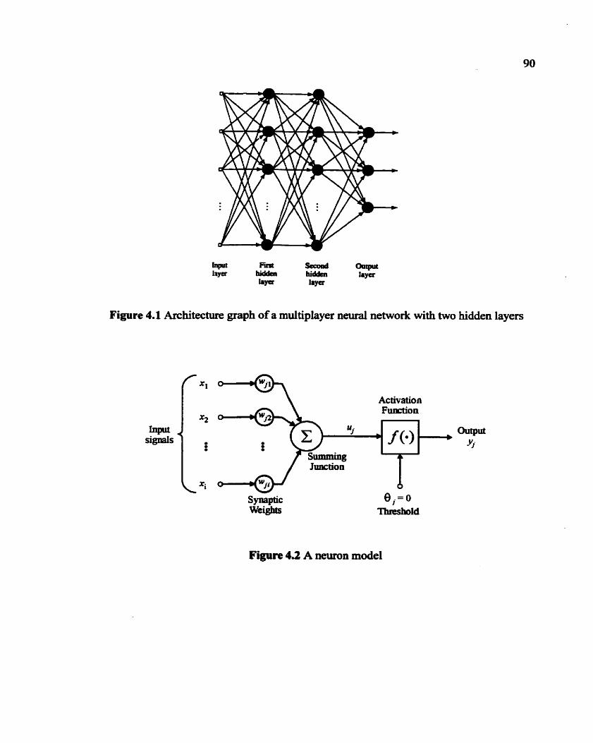
Figure 4.1 Architecture graph of a multiplayer neural network with two hidden layers
signals
\ Activation
Synaptic Weights
Figure 4.2 A neuron model
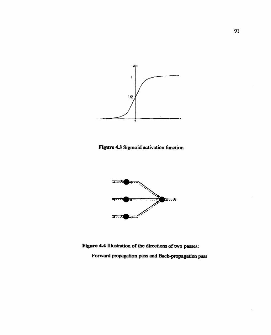
Figure 4 3 Sigmoid activation kction
Figure 4.4 Illustration of the directions of two passes:
Forward propagation pass and Back-propagation pass
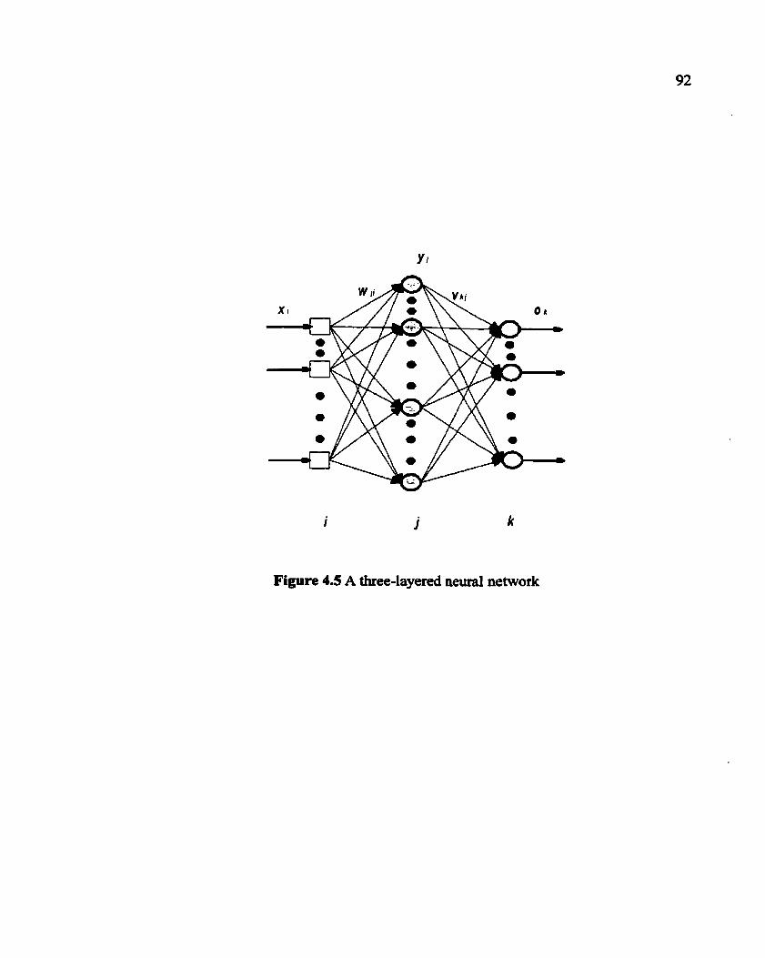
i i k
Figure 4.5 A three-layered neural network
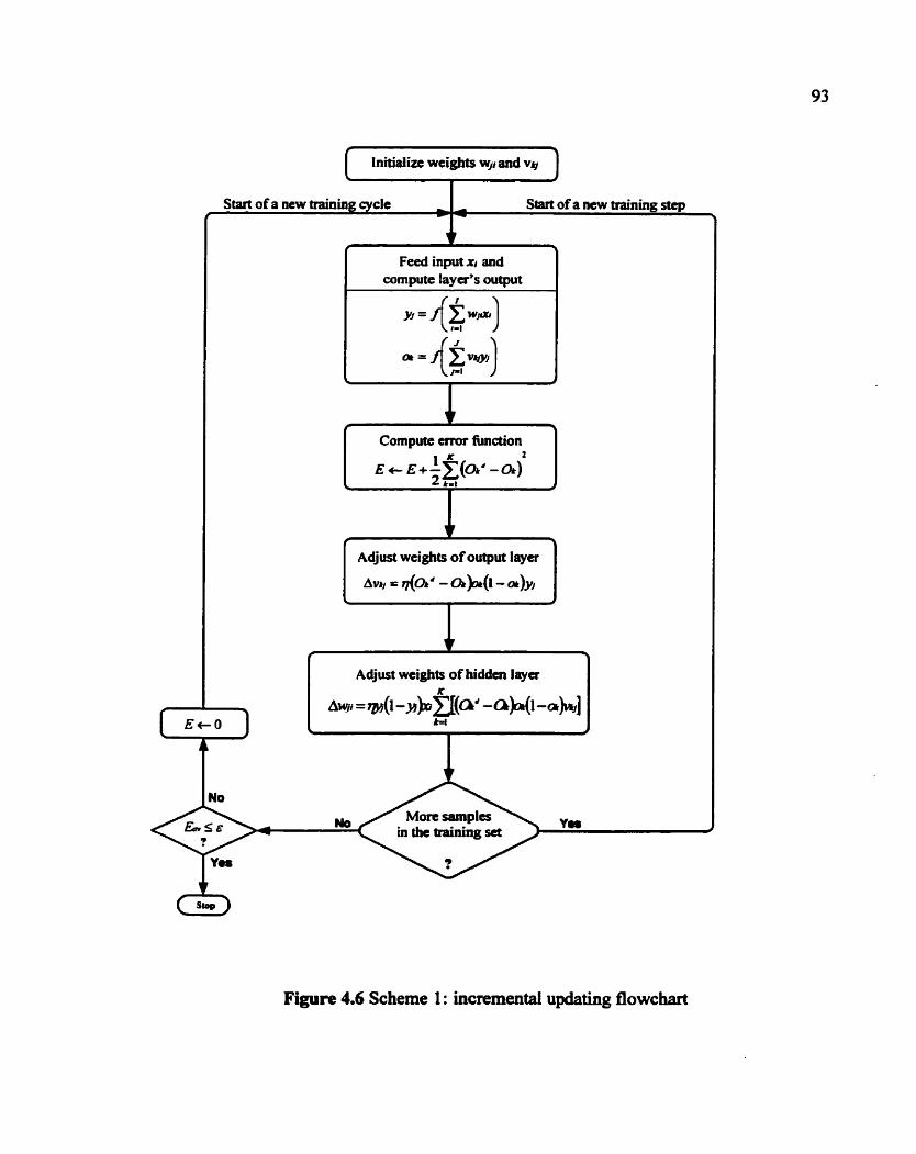
I tnitidizc weights w, and v4 1
Figure 4.6 Scheme 1 : incremental updating flowchart
Start of a new training cycle f b 4
Start of a new training step
E - 0
v f \
Feed input xi and compute layer's output
b J
P 3
Compute error hction 1 2
E t E + - ~ ( O I ' - ~ ) < 2 &-I - J
v f \
Adjust weights of output layer
Auk, = r l ( ~ ' - &h)a(l- \ 4
v f l \
Adjust weights of hidden laya K
AW~ = q ~ ( 1 -s)ux[(~ -a)a(l -a))ij]
&==I \ I
A
No More samples Yes #
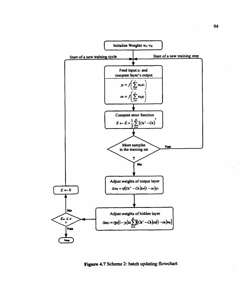
I initiatii Weights wjt ve I
Figure 4.7 Scheme 2: batch updating flowchart
Start of a new training cycle f
Start of a new training step C 4
v I 3
Feed input xi and compute layer's output
,!! =f($w)
a = f(g Vk,Yj)
k /
f \ Compute error function
1 " : 2
E t E+-x(a* -aI) 2 h, #
Ys,
No
v I 9
Adjust weights of output layer
Ava = dot' - h)or(l- J \
v No r \
Adjust weights of hidden layer K
= m(~-Mbu(ad -aM~-a)ro] h l
J
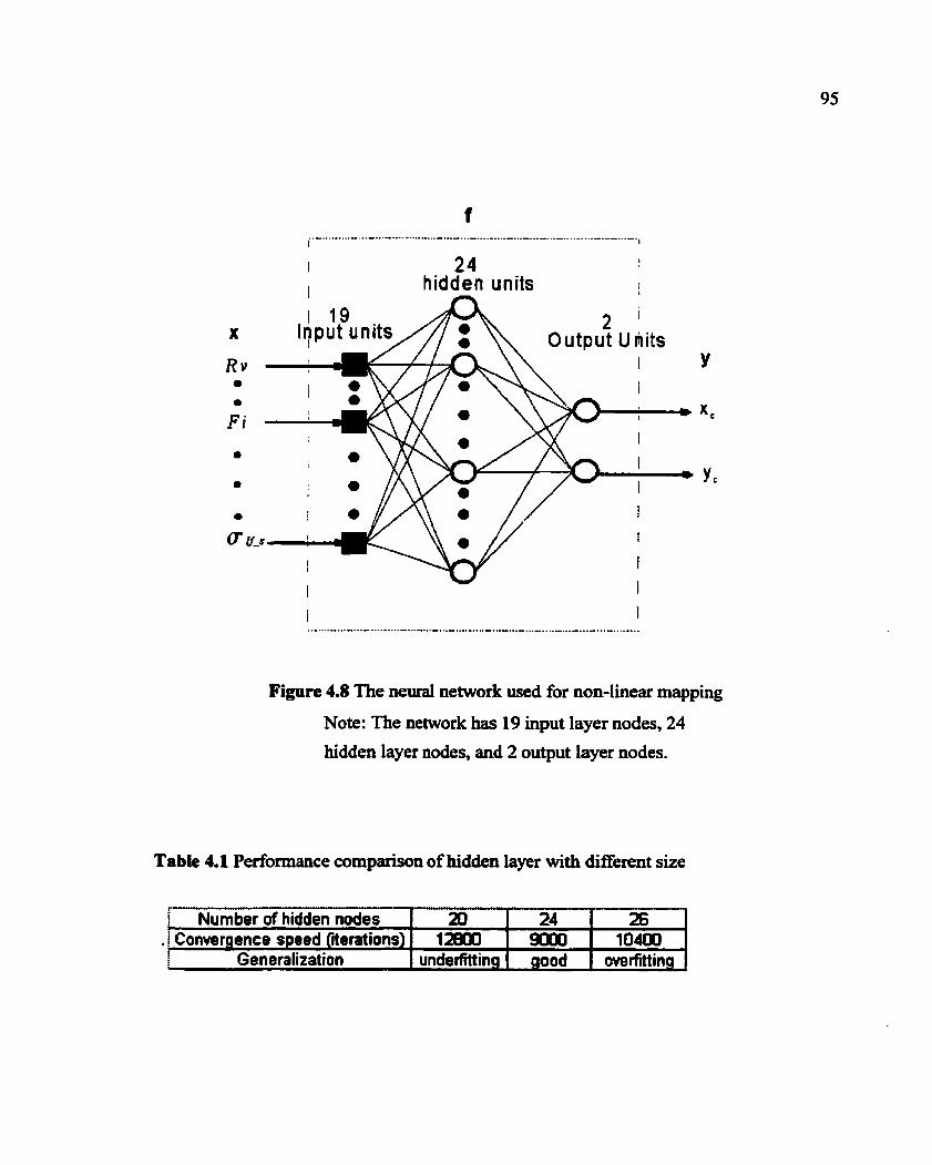
I 24 I hidden n units
Figure 4.8 The neural network used for non-linear mapping
Note: The network has 19 input layer nodes, 24
hidden layer nodes, and 2 output layer nodes.
Table 4.1 Performance comparison of hidden layer with different size
- j Number of hidden nodes 20 24 26
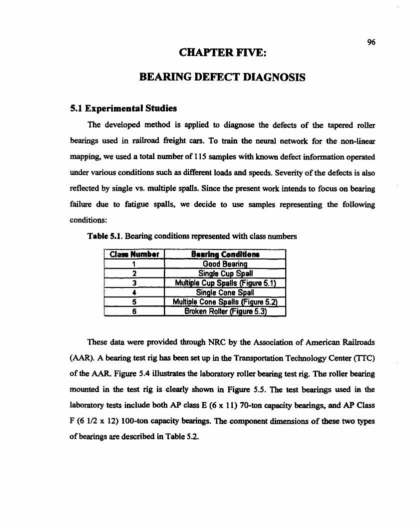
CHAPTER FIVE:
BEARING DEFECT DIAGNOSIS
5.1 Experimental Studies
The developed method is applied to diagnose the defects of the tapered roller
bearings used in railroad fkight cars. To train the neural network for the non-linear
mapping, we used a total number of 1 15 samples with known defect information operated
under various conditions such as different loads and speeds. Severity of the defects is also
reflected by single vs. multiple spas. Since the present work intends to focus on bearing
failure due to fatigue spalls, we decide to use samples representing the following
conditions:
Table 5.1. Bearing conditions represented with class numbers
These data were provided through NRC by the Association of American Railroads
(AAR). A bearing test rig has been set up in the Transportation Technology Center (TTC)
of the AAR. Figure 5.4 illustrates the laboratory roller bearing test rig. The roller bearing
mounted in the test rig is clearly shown in Figure 5.5. The test m g s used in the
laboratory tests include both AP class E (6 x 11) 70-ton capacity bearings, and AP Class
F (6 1R x 12) 100-ton capacity bearings. The component dimensions of these two types
of bearings are described in Table 5.2.
f Clm Numbor 1- 2
a
3 4
f 5 6
Boaring Conditions Good Bearing
Single Cup Spall Multiple Cup Spalls (Figure 5.1)
Single Cone Spall Multiple Cone Spalls (Figure 5.2)
Broken Roller Figure 5.3)
97
Each AP class bearing (EBtF) are embedded with defects of different types as listed
in Table 5.1. Experiments are performed with two separate radial loads representing
empty and Mly loaded fieight car:
Type E bearings: 8,000 lb. and 27,500 lb.
Type F bearings: 8,000 ib. and 33,000 lb.
Each test is conducted at different train speeds ranging fkom 30 to 80 miles per hour
(MPH) at increment of 10 miles per hour.
Test data are collected from acoustic sensors and accelerometers in parallel for all
bearings under test. Analog signals are digitized with a sampling rate of 270 kHz. The
digital signals are stored in files, each of which contains 540,000 points representing 2
seconds of signal collection time. Tachometers are also used to measure the exact shaft
rotation speed to provide a reference for synchronization.
5.2 Feature Selection
The obtained vibration signals are processed and analyzed through time domain,
fiequency domain and segmentation analyses. A total number of nineteen feature
parameters are calculated for measured signals. Time domain parameters include Root
Mean Square value (Rv), Peak value (Pk), Crest factor (Cf), Kurtosis value (Kv),
Clearance factor (Clf) and Impulse factor (If). They can be used to indicate either the
severity of the bearing defects or the spikiness of the vibration amplitude associated with
the defect-induced impulses.
Frequency index (Fi) is the parameter extracted h m fiequency domain proposed to
highlight significant fiequency contents that may be associated with the bearing defect
characteristics hquencies [Sun, et al., 19981. Although the defect characteristic
fkequencies could be used to help determine the location of the defect, automatic
98
detection of impulses at these fkequencies is not a simple task. This is because frequency
spectra often show much stronger peaks at much higher fiequencies representing high
order structural resonance compared to those at the characteristic fiequencies. Vibrational
energy of the bearing spreads across a wide fkquency band and can be easily buried in
the noise. Figure 5.6 shows the fhquency spectrum of a bearing with outer race defect.
The dominant fkequency can be seen to be around 4300Hz which is far beyond the range
of the roller passing outer race fkquency as shown in Table 2.1. No explicit relations
between the spectrum and the defect characteristic kquencies can be constructed in the
case. Therefore, it is not advised to depend solely on the fiequency spectrum, which
necessitates the pattern recognition analysis for more reliable diagnosis.
Segmentation analysis is applied to characterize non-stationary signals through
segmenting the signal into quasi-stationary components based on the understanding of
bearing dynamics. Impulses can only be generated from the passage of defects when they
are inside the load zone. Defects located on different bearing components will generate
impacts with different fkquencies and modulation patterns when passing through the
load zone. Correlation exists between the location of the defects and the impulse patterns
observed in the vibration signal. We decide to divide the signal in one shaft or cage
revolution into six segments, so that at least one segment will be completely inside the
load zone and one completely outside of the load zone. Segmentation parameters are
determined based on the calculation of standard deviation of the time domain parameters
in various segments using cage hquency and shaft fkquency respectively. A segmented
vibration signal obtained fbm bearing with h e r race defect and the spectra of each
segment are illustrated in Figure 5.7. It is obvious that the peaks in the spectra of the last
two segments are much more dominant than the those in other four segments, which
corresponds to the impulse generating region in the time domain waveform.
99
5.3 Results of the Artificial Neural Network
Nineteen parameters are first calculated for each measured signal of the 1 15 samples
to form the feature space, as listed in Table 5.3. These parameters are then normalized
and used as input to train the neural network to perform the non-linear mapping as
discussed in chapter 4. Before training, it is often usefhl to scale the inputs and targets so
that they always fall within a specified range. This preprocessing is helpful for efficient
and stable behavior of the training process. We choose to scale all numbers such that they
fall into the range of a sigmoid function, i.e., between 0 and 1. The minimum and
maximum values of each feature parameter for the total 115 samples, that is, the
minimum and maximum of each column in Table 5.3 are used to normalize the column
into the sigrnoid range. These values are also exploited in normalizing the test data for
diagnosis as detailed later. Each training data set consists of the normalized nineteen
input parameters and the specified cluster centers as target outputs of the network as
shown in Table 5.4.
An error criterion of 0.01 is achieved through a trial and error approach. The
network training was pursued for 9,000 iterations when the error criterion was reached.
The actual outputs at the end of training are compared with the target outputs and listed in
Table 5.5. The averaged error fhction Em of the trained network is calculated to be 0.009
also shown in the table, which fkther co- that the learning has converged to the
expected criterion. If the error criterion is chosen to be 0.005, the network converges after
16,000 iterations and only leads to 5% reduction of the error hct ion Em. An error
criterion of 0.02 was also tested, the network learning converged after 6,000 iterations.
However, with the value of Em being 0.019 the samples belonging to different classes
were not well clustered in the classification space and had some overlapping.
Feature extracttion without segmentation parameters fiom the same bearing was
performed to compare with the developed method. The same experimental data were
100
used for the pattern recognition. The learning process took the same network more than
40,000 iterations to converge to the same error criterion.
After the network training was complete, the actual network outputs were plotted on
a 2D space and the mapping result is shown in Figure 5.8, where the Arabic numbers
represent different bearing conditions as listed in Table 5.1. The black dots in the
classification space represent the designated cluster centers. Although their arrangement
was somewhat arbitrary, we placed them evenly on a unit circle in the first quadrant of a
2D space as shown in Figure 5.9. There were three reasons for this configuration. Firstly,
a unit circle was chosen so that the outputs will fall into the range of a sigmoid function,
that is, between 0 and 1. Secondly, a larger circle does not necessarily lead to a better
clustering effect. In fact, although the between-class distance may increase with the
diameter, the within-class distance may also increase. Consequently, class separability
will not be improved. The third reason states that if cluster centers were arrayed on a unit
square in the first quadrant of a 2D space as shown in Figure 5.10, the convergence of the
network took longer. Also, some regions are left unexplored because the mapped samples
could not distribute evenly in the first quadrant. Finally, the coordinates of the cluster
centers, that is, the desired [xc are chosen to be:
It can be observed from Figure 5.8 that samples belonging to different classes are
separated in different regions and clustered around their own pre-defined cluster centers
in the classification space. The neural network has successfully performed the high
fidelity dimension reducing non-linear mapping. The intra-class transformation [Sun, et
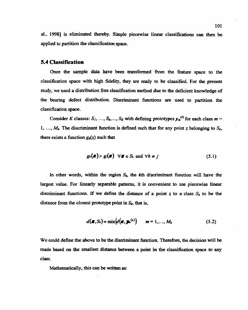
101
al., '19981 is eliminated thereby. Simple piecewise linear classifications can then be
applied to partition the classification space.
5.4 Classification
Once the sample data have been transformed h m the feature space to the
classification space with high fidelity, they are ready to be classified. For the present
study, we used a distribution h e classification method due to the deficient knowledge of
the bearing defect distribution. Discriminant hc t ions are used to partition the
classification space.
Consider K classes: S,, . . . , Sk,. . ., SK with defining prototypes y,,,(k' for each class rn =
1, . . ., ktk. The discriminant bc t ion is defined such that for any point z belonging to Sk,
there exists a function gdz) such that
g k ( ~ ) > ~ ( ~ ) VZ €St and tlk* j (5-1)
In other words, within the region Sk, the kth discriminant function will have the
largest value. For linearly separable patterns, it is convenient to use piecewise linear
discriminant hctions. If we d e h e the distance of a point z to a class Sk to be the
distance fiom the closest prototype point in Sk, that is,
We could define the above to be the discriminant function. Therefore, the decision will be
made based on the smallest distance between a point in the classification space to any
class.
Mathematically, this can be written as:
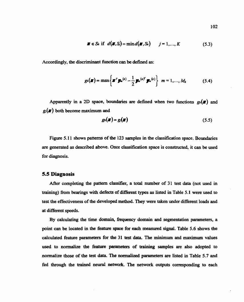
Accordingly, the discriminant hct ion can be defined as:
Appareny in a 2D space, boundaries are defined when two functions @(z) and
g j ( ~ ) both become maximum and
= d=) (5.5)
Figure 5.1 1 shows patterns of the 123 samples in the classification space. Boundaries
are generated as described above. Once classification space is constmcted, it can be used
for diagnosis.
5.5 Diagnosis
After completing the pattern classifier, a total number of 31 test data (not used in
training) from bearings with defects of different types as listed in Table 5.1 were used to
test the effectiveness of the developed method. They were taken under different loads and
at different speeds.
By calculating the time domain, fnquency domain and segmentation parameters, a
point can be located in the feature space for each measured signal. Table 5.6 shows the
calculated feature parameters for the 31 test data. The minimum and maximum values
used to normalize the feature parameters of training samples are also adopted to
normalize those of the test data. The normalized parameters are listed in Table 5.7 and
fed through the trained neural network. The network outputs corresponding to each
103
measured signal were plotted in the classification space denoted by different symbols as
shown in Figure 5.11. The results show that all the testing data were correctly recognized.
The developed methdd is very effective in bearing defect diagnosis.
S/N 54900 *. 3 UULTIRECUPSPUW TEST BRG #9 b
Figure 5.1 Multiple cup spalls
Fi gum 5 2 Multiple cone spalls
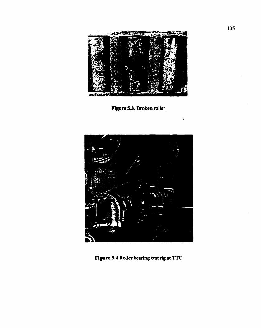
Figure 5.4 Roller bearing test rig at TI%
Figure 5.3. Broken roller
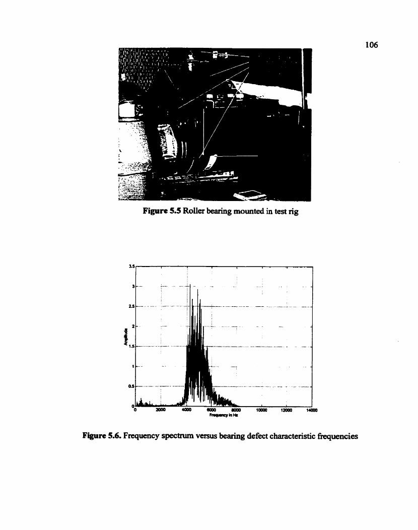
F w In #
Figure 5.6. Frequency spectrum versus bearing defect characteristic fraluencies
Figure 5.5 Roller bearing mounted in test rig
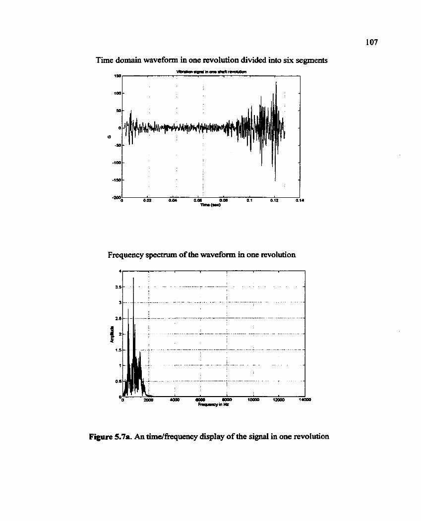
Time domain waveform in one rewolution divided into six segments
Fmquency spectrum of the waveform in one revolution
Figure 5.7a. An time/fiequency display of the signal in one revolution
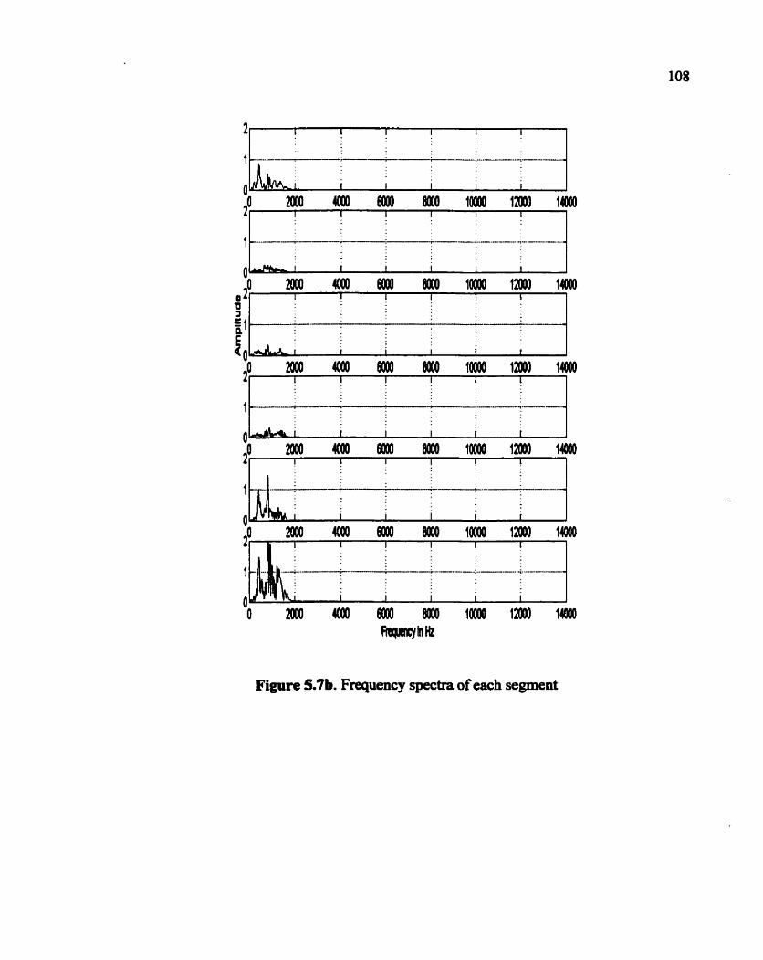
Figure 5.7b. Frequency spectra of each segment
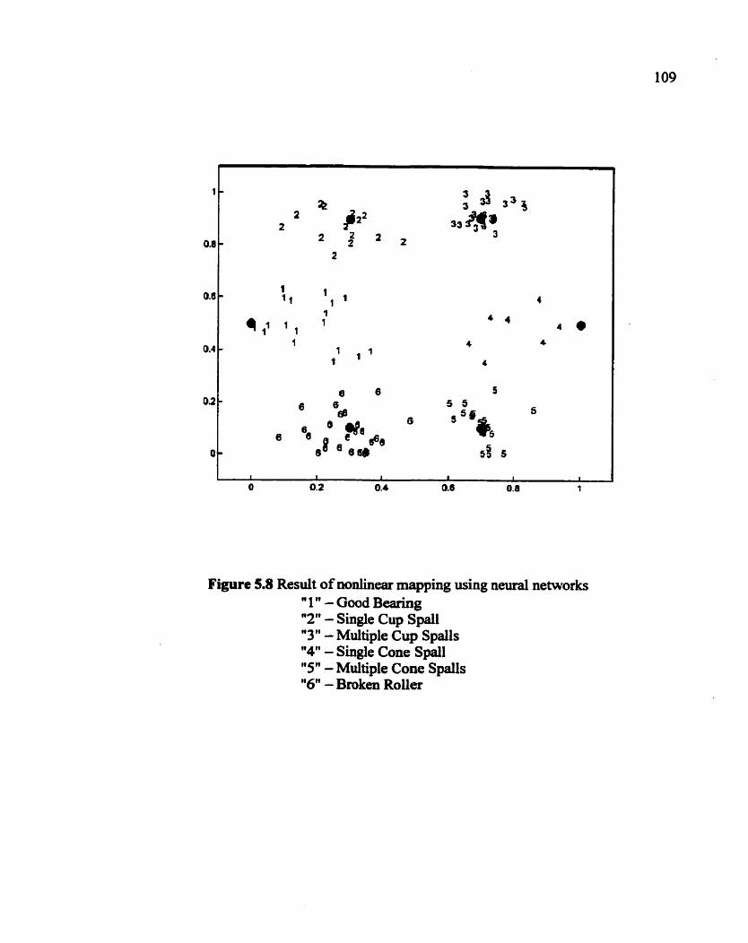
Figure 5.8 Result of nonlinear mapping using neural networks " 1 " - Good Bearing "2" - Single Cup Spall "3 " - Multiple Cup Spalls "4" - Single Cone Spall "5" - Multiple Cone S p a s "6" - Broken RoUer
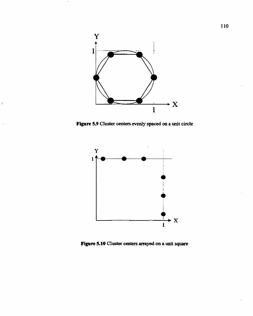
Figure 5.9 Cluster centers evenly spaced on a unit circle
1
Figure 5.10 Cluster centers arrayed on a unit square
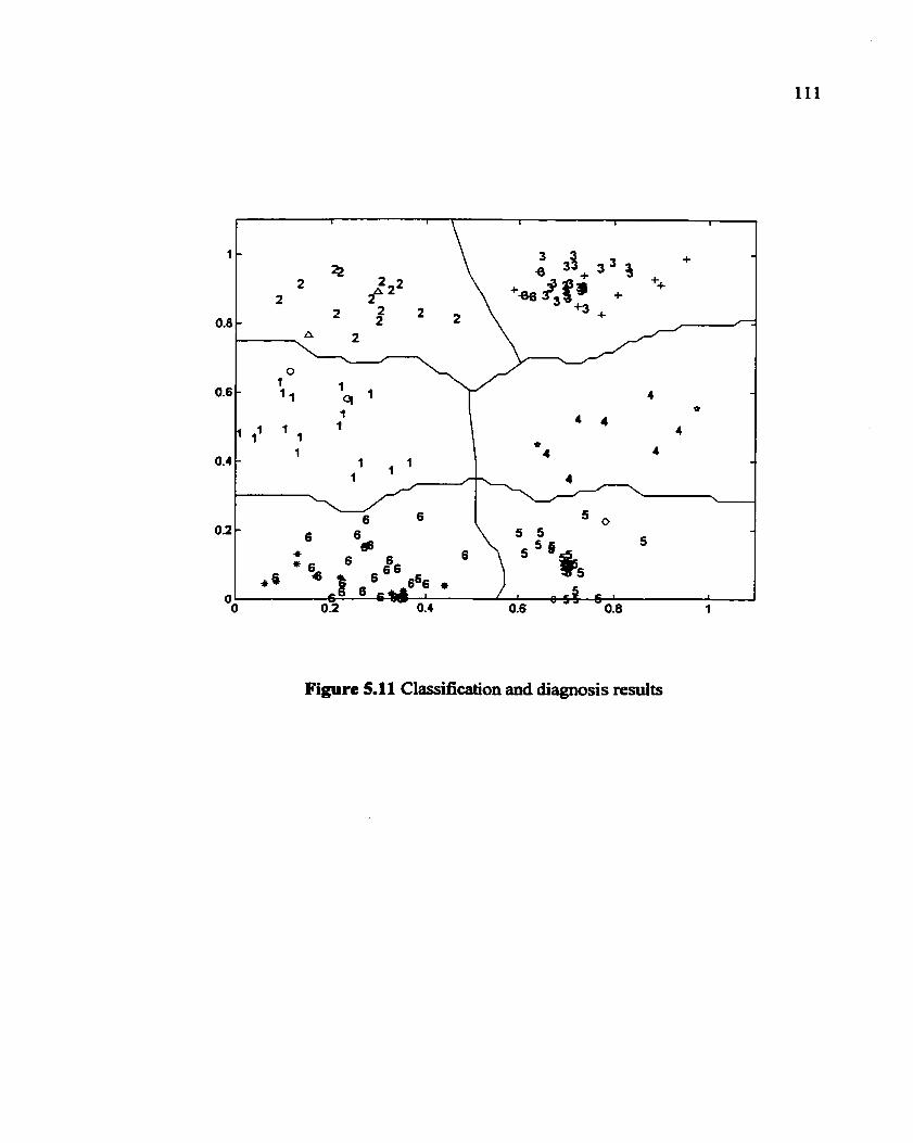
Figure 5.11 Classification and diagnosis results
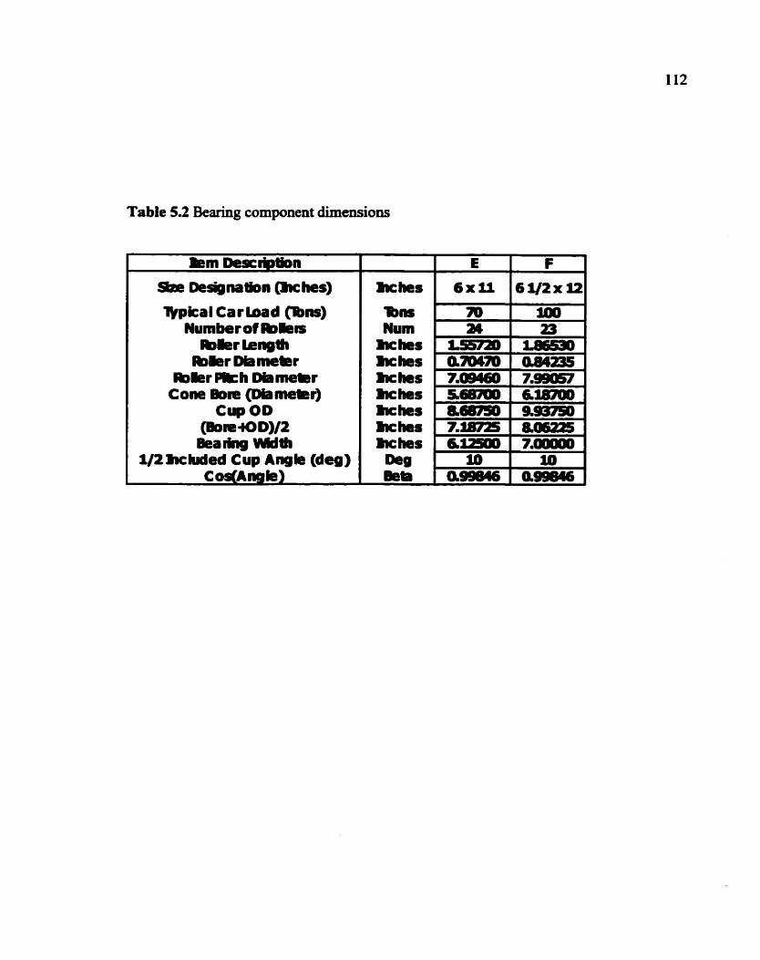
Table 5.2 Bearing component dimensions
bem Description
Sae Designation (k hes)
Wpical Carload pns) Number of RPlem
Cbler lenglh lbler D&mebr
lblerPRh DiameBr Cone BOR (DiaMBOer)
Cup OD @--D)/2 Bearing HMlh
1/2 -hided Cup Angle (deg) Cos(Angle)
hches
'Ibm Num
hches hches hches hches hches hches hches
Deg Beta
E
6 x l l
;FD a4 m am470 7.- S68;F#)
7.U3725 6-
10 QM
F
61/2xl2
100 23
lS530 .
7.- -6-
AS3750 80622s 7.00000 3.0
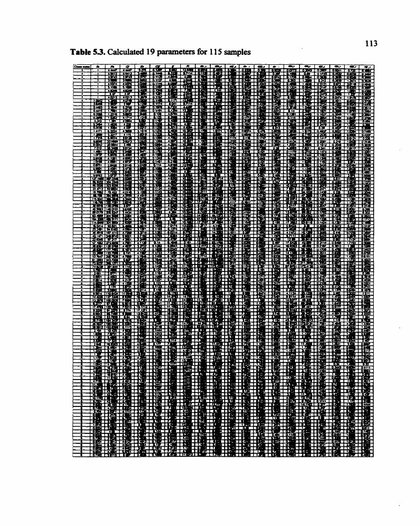
Table 53. Calculated 19 parameters for 1 15 samples
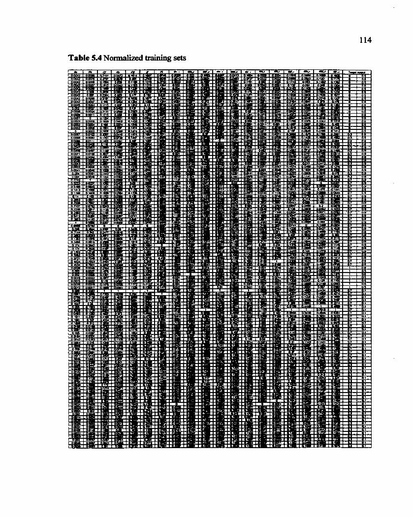
Table 5.4 Normalized training sets
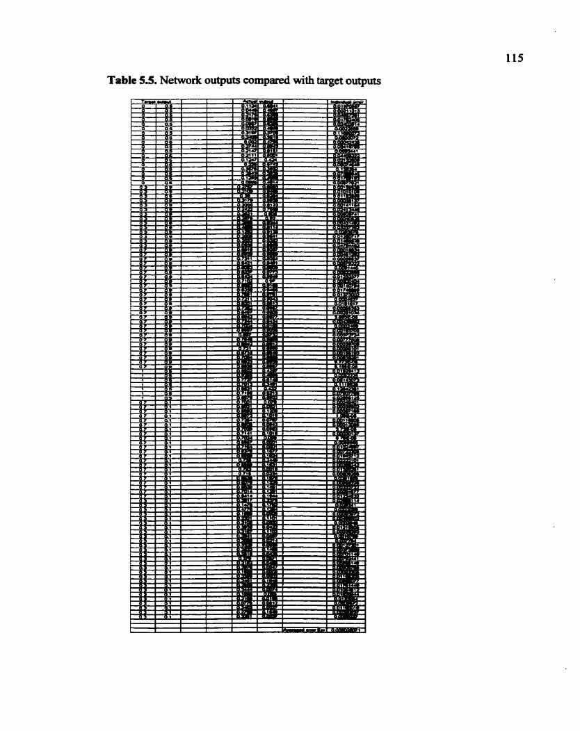
'able 5.5. Network outputs compared with target outputs
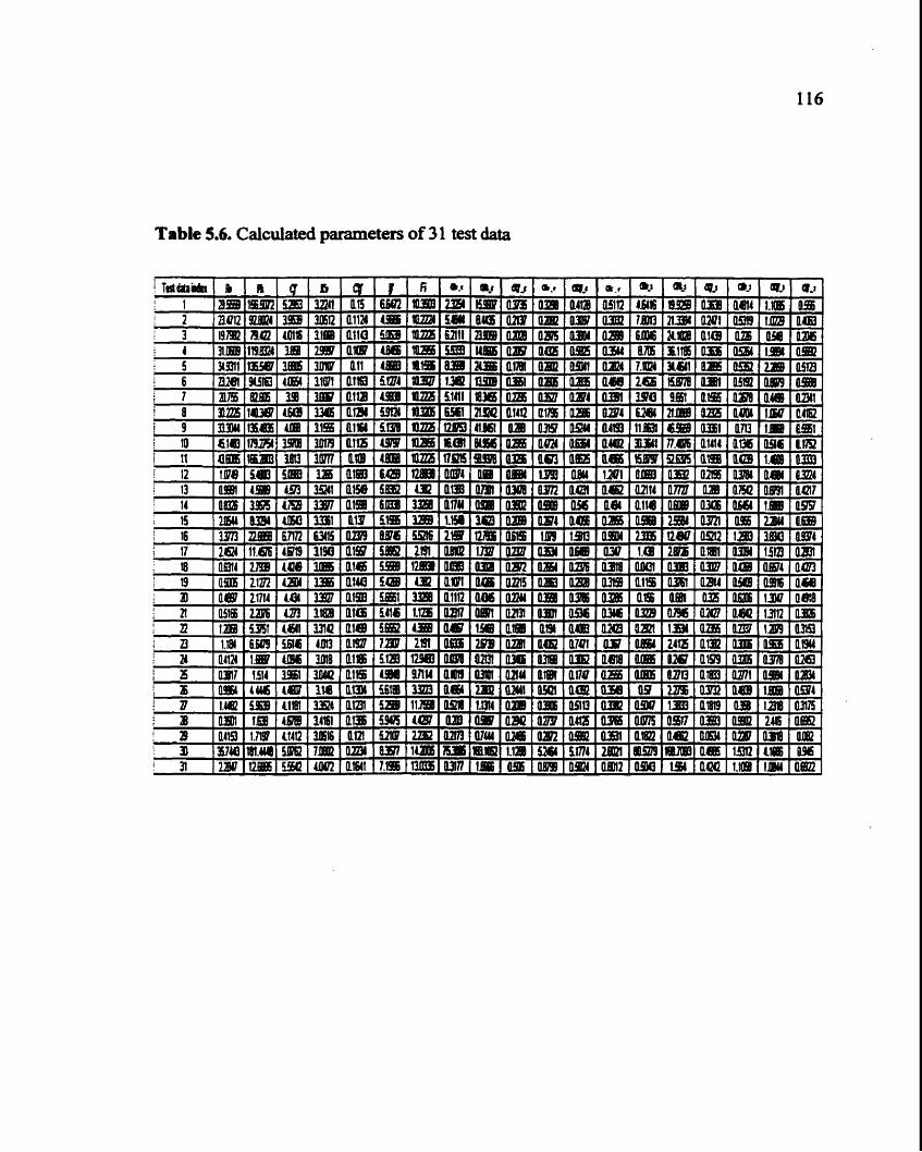
Table 5.6. Calculated parameters of 3 1 test data
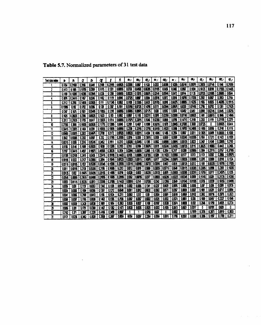
Table 5.7. N o r m M parameten of 3 1 test data
CHAPTER SIX:
CONCLUSION AND FUTURE WORK
6.1 Summary of Results Obtained
The signal processing and pattern recognition techniques described in chapters 3,4,
and 5, were applied to vibration signals obtained from rolling element bearings used in
railway hight cars.
Vibration signals obtained from bearings were processed and analyzed through time
domain, fiequency domain and segmentation analyses. T i e domain parameters include
Root Mean Square value (Rv), Peak value (Pk), Crest factor (Cf), Kurtosis value (Kv),
Clearance factor (Clf) and Impulse factor (If). They provide information such as the
spikiness and the energy level of the vibration signals. Frequency index (Fi) is the
parameter extracted from kquency domain proposed to highlight significant frequency
contents that may be associated with the bearing defect characteristics fkquencies.
Earlier work on pattern recognition for bearing defect diagnosis using these parameters
showed promising results and was simple to implement [Sun et al., 19981.
The sensitivity and reliability of the pattem recognition analysis is fUrther improved
by including the newly developed segmentation parameters. Since the vibration signal of
a bearing with defects is generally non-stationary, segmentation d y s i s can be applied
to feature the description of such a signal through segmented quasi-stationary
components. Based on the observation that impuises can only be generated from the
passage of the defect contacting the mating surfaces under load, vibration signals present
certain patterns associated with def- inside or outside of the bearing load zone. Defects
located on different bearing components will generate impacts when passing through the
load zone with different fkquencies and modulation patterns. A correlation exists
119
between the variation pattern of signals and the location of defects on the bearing
components and impulses modulated with the shaft or cage frequency can be detected.
For the bearings studied in this work, the radial loads cause a stress distribution
over an angle range of about 120 degrees. A fixed-length segmentation scheme is used in
order to reduce the computational expense of the process. Signals in one shaft revolution
and cage revolution are evenly divided into six segments respectively so that at least one
segment will be completely inside the load zone and at least one segment can be
completely outside of the load zone. Descriptive features of these signal segments can be
calculated through time domain parameters. Segmentation parameters are thus
determined based on the calculation of standard deviation of the time domain parameters
among six segments. They can directly reflect the variation of vibration patterns
associated with the bearing load zone. The segmentation parameters referenced in both
shaft and cage rotations are employed to participate in constructing the feature space.
Segmentation parameters, together with the existing time and fkequency domain
parameters are used to construct the feature space. Thus the find feature space is
composed of 19 dimensions. A three-layered artificial neural network is used to
accomplish the nonlinear mapping fiom the 19-dimensional feature space to the 2-
dimensional classification space. Artificial neural networks allow us to construct
complicated non-linear relations between input and output when analytical description is
not available.
The ANN is chosen to have three layers since three-layered networks are
s a c i e n t for representing the non-linear relations between the input and output and they
have relatively simple architecture. The error back-propagation algorithm is used to train
the neural network. The same sigmoid activation h c t i o n in the form of a logistic
function is chosen for all the hidden and output neurons of the network as it allows the
network to learn non-linear relationships between input and output vectors. The nineteen
120
feature parameters extracted fiom vibration signals are fed as inputs to the network and
the output contains the corresponding coordinates in the 2D classification space. The
cluster centers are evenly spaced on a unit circle in the first quadrant of a 2D space in
order to locate the desired outputs associated with each of the classes. The neural network
is trained with known input sets each of which consists of 19 parameters and the
corresponding desired outputs that are the specified cluster centers. The finally obtained
optimal architecture of the network is 19-24-2 through a trial and error approach. A
heuristic technique, variable learning rate, is adopted in order to accelerate the
convergence of back propagation learning. A momentum is also incorporated to b l p
speed up convergence, and achieve a more efficient and reliable learning profile.
A total number of 115 samples with known defect information operated under
various conditions such as different laods and speeds are used to train the network.
Severity of the defects is also reflected by single vs. multiple spalls. The network training
was pursued for 9,000 iterations when an error criterion of 0.01 was reached. Feature
parameters without the segmentation parameters extracted fiom the same bearing was
also investigated. It took the same network more than 40,000 iterations to converge to the
same error criterion. The mapping result shows that the corresponding outputs in the
classification space are completely separated in different regions and clustered around the
prescribed centers associated with bearing in different conditions. The artificial neural
network has successfidly performed the high fidelity dimension reducing non-linear
mapping. The intraclass transformation is eliminated thereby. Successll mapping
allows application of the simple piecewise linear boundaries.
A total number of 3 1 test data (not used in training) fiom bearings with defects of
different types as listed in Table 5.1 were used to test the effectiveness of the developed
method. They are taken fiom bearings under different operating conditions. By
calculating the time domain, frequency domain and segmentation parameters of the
121
signals, these samples can be located in the feature space. Fed through the trained neural
network, each test sample is identified on the classification space. The classification
results show that they are all correctly recognized.
In summary, the developed method based on pattern recognition analysis has
improved the sensitivity and reliability in bearing fault diagnosis by including the
segmentation parameters. The successful non-linear mapping through the neural network
eliminates intra-class transformation process. The result shows the method is simple and
effective. It is suitable for the development of automatic monitoring and diagnostic
systems.
6.2 Limitations of the Present Method and Directions for Future Work
Although the present method accurately has recognized bearing conditions, the
results were obtained using experimental data. In actuality, we deal with bearings
mounted on moving trains. Vibration signals obtained fiom this environment are
expected to have diEerent characteristics than those obtained fiom a test rig in the lab.
Future work will be directed towards investigating the reliability of the existing method
diagnosis. Improvement, if any, needs to be made to further increase the sensitivity of the
method to non-defect related characteristics.
Also in this work, we focused on detecting and diagnosing bearing defects caused
by fatigue spalling as it is the predominant bearing failure mode. Further studies need to
be conducted to include other bearing failure modes.
REFERENCES
R.J. ALfiredson and J. Mathew, "Frequency domain methods for monitoring the condition
of rolling element bearingsy'. Mechanical Engineering Transactions, Vol. ME10, No.2,
The Institution of Engineers, Australia, July 1985(a), pplO8- 1 12.
R. J. Alhdson and J. Mathew, "Time domain methods for monitoring the condition of
rolling element bearings". Mechanical Engineering Transactions, Vol. ME 10, No.2, The
Institution of Engineers, Australia, July 19850, ppl02-117.
I. E. Alguindigue, Anna Loskiewicz-Buczak, and Robert E. Uhrig, "Monitoring and
Diagnosis of Rolling Element Bearings Using Artificial Neural Networks". IEEE
Transactions on Industrial Electronics, VOL. 40, NO. 2, pp. 209-217, April 1993.
I. E. Alguindigue and Robert E. Uhrig, "Automatic Fault Recognition in Mechanical
Components Using Coupled Artificial Neural Networks". IEEE International Conference
on N e d Networks, Part 5 (of 7), Jun 27-29, VOL. 5, 1994, Orlando, FL, USA, pp
3312-3317.
G. B. Anderson, J. E. Cline, D. H. Stone, and R. L. Smith, "A New Detection Technique
to Identify Defective Railroad Bearings". American Society of Mechanical Engineering,
Rail Transportation Division (Publication) RTD Rail Transportation, Proceedings of the
1996 ASME International Mechanical Engineering Congress and Exposition, Nov 17-22,
1996, Vol. 12.
Y. A. Azovtsev, A. V. Barkov, and I. A. Yudin, "Automatic diagnostics and condition
prediction of rolling element bearing using enveloping methods". Vibration Institute lgh
Annual Meeting, June 20-23,1994.
123
D. C. Baillie and J. Mathew, "A Comparison of Autoregressive Modeling Techniques
for Fault Diagnosis of Rolling Element Bearingsy'. Mechanical Systems and Signal
Processing, VOL. 10, NO. 1, Jan 1996, pp 1-17.
R H. Bannister, "A review of rolling element bearing monitoring techniques".
1.MECH.E Conference on Condition Monitoring of Machinery and Plant, 1985, ppl l-24.
B. G. Batchelor, "Pattern Recognition". Plenum Press, New York, 1978.
G. Bodenstein and H. M. Praetorious, "Feature extraction from the electroencephalogram
by adaptive segmentation", Proceedings of the IEEE, V65, No. 5, pp642-652, May 1977.
S. Braun and B. Datner, "Analysis of rollerhall 'bearing vibrations". ASME J.
Mechanical Design, 1979, 101, pp. 1 18-125.
Y. Chiou, Massoud S. Tavakoli, and Steven Liang, "Bearing fault detection based on
multiple signal features using neural network analysis". Proc. 10th Int, Modal Analysis
Cod., San Diego, CA, 1992, pp. 60-64.
H. C. Choe, Yulun Wan, and Andrew K. Chan, "Neural Pattern Idenscation of Railroad
Wheel-bearing Faults from Audible Acoustic Signals: Comparison of FFT, CWT, and
DWT features". Proceedings of SPIE - The Intenrational Society for Optical Engineering
Wavelet Applications IV, VOL. 3078, April 22-24, 1997, Orlando, FL, USA, pp 480-
496.
J. Courrech, 'mew techniques for fault diagnosis in rolling element bearings".
Proceedings of the 40' Mechanical Failures Prevention Group, Maryland, April 1985, pp
83-9 1.
124
G. Cybenko, "Approximation by superpositions of a sigmoidal hction". University of
Illinois, Urbana, 1988.
D. Dyer and R. M. Stewart, "Detection of rolling element bearing damage by statistical
vibration analysis". Transactions of the American Society of Mechanical Engineers,
Journal of Mechanical Design, Vol. 100, April 1978, pp 229-235.
R. L. Eshleman, "The role of sum and difference kquencies in rotating machinery fault
diagnosis". Proceedings of the 2"d International Conference on Vibrations in rotating
machinery, 1.Mech.E. paper C272/80,1980, pp 145-149.
R L. Florom, "Improved wayside train inspection program". Town Hall Meeting,
Association of American Railroads, Chicago Technical Center, Chicago, Illinois, June
15, 1994.
P. K. Gupta, "Transient ball motion and skid in ball bearings". Transactions of the
American Society of Mechanical Engineers, Journal of Lubrication Technology, April
1975, pp 261-269.
P. K. Gupta, "Dynamics of rolling element bearings Part I: Cylindrical Roller Bearing
Analysis". Transactions of the American Society of Mechanical Engineers, Journal of
Lubrication Technology, Vol. 10 1, July 1979(a), pp 293-304.
P. K. Gupta, c4Dynamics of rolling element bearings Part XI: Ball Bearing Analysis".
Transactions of the American Society of Mechanical Engineers, Journal of Lubrication
Technology, Vol. 101, July 1979(b), pp 305-3 1 1.
125
P. K. Gupta, "Dynamics of rolling element bearings Part ID: Ball Bearing Analysis".
Transactions of the American Society of Mechanical Engineers, Journal of Lubrication
Technology, Vol. 10 1, July 1979(c), pp 3 12-3 18.
P. K. Gupta, "Some dynamic effects in high-speed solid-lubricated ball bearings".
Proceedings of the ASLW ASME Lubrication Conference, New Orleans, Louisiana,
October 5-7, 198 1.
P. K. Gupta, J. F. Dill, and H. E. Bandow, "Dynamics of rolling element bearings:
Experimental validation of the DREB and RAPIDREB computer programs".
Transactions of the American Society of Mechanical Engineers, Journal of Tribology,
Vol. 107, Jan 1985, pp 132-137.
0. G. Gustafsson and T. Tallian, "Detection of damage in assembled rolling bearings",
Transaction of the American Society of Lubrication Engineers, Vol. 5, 1962, pp 197-209.
L. G. Hampson, "Diagnostic checks for rolling bearings". Proceedings of a seminar
organized by the Institute of Mechanical Engineers, Rolling Element Bearings, Feb. 22,
1983.
Simon Haykin, " N e d networks - a comprehensive foundation". Macmillan College
Publishing Company, NJ, USA, 1994.
M. J. Hine, "Absolute ball bearing wear measurements from SSME turbopump dynamic
signals". Journal of Sound and Vibration, Vol. 128, No. 2, 1989, pp 3 2 1 -3 3 1.
P. S. Houghton, "Ball and Roller Bearings". Applied Science Publishers Ltd, Ripple
Road, Barking, Essex, England.
126
I. M. Howard and G. W. Stachowiak, "Detection of surface defects in rolling contact
bearings". The Institution of Engineers, Australia, Mechanical Engineering Transactions,
Vol. 13, 1989, pp 158-164.
I. Howard, "A review of rolling element bearing vibration - detection, diagnosis and
prognosis", Defense Science and Technology Organization, Australia, October, 1994.
H. Huang and H. P. - Ben W a g , "An Integrated Monitoring and Diagnostic System for
Roller Bearings". The International Journal of Advanced Manufacturing Technology,
VOL. 12, No. 1, pp. 37-46, 1996.
T. Igarashi and H. Hamada, "Studies on the vibration and sound of defective rolling
element bearings (Third Report: Vibration of ball bearing with multiple defects)".
Bulletin of the Japanese Society of Mechanical Engineers, Vol. 28, No. 237, March 1985,
pp 492-499.
V. Jammu and Th. Walter, "Standoff Bearing Fault Detection Using Directional
Microphones and Unsupe~sed Neural Networks", Shock and Vibration Digest, VOL.
29, 1997, pp 17-25.
M. Karkoub and Ali Elkarnei, "Modelling pressure distribution in a rectangular gas
bearing using neural networks". Tribology International, Vo1.30, N0.2, 1 99 1, pp. 1 39- 1 50.
J. E. Keba, "Component test results h m the bearing Life improvement program for the
space shuttle main engine oxidizer turbopumps". Proceedings of the 3d International
Symposium on Rotating Machineryy Honolulu, HIy 1990, pp 303-3 1 8.
127
P. E. Keller, Richard T. Kouzes, Lars J. Kangas, Sherif Hashem, "Neural network based
sensor systems for manufacturing applications". Advanced Information Systems and
Technology Conference, Williamsburg, VA, USA, 28-30 March, 1994.
R. J. Kershaw, "Machine Diagnostics with Combined Vibration Analysis Techniques".
Proceedings of the 41' Meeting of the Mechanical Failures Prevention Group, October
1986, pp 160- 168.
A. F. Khan, "Condition monitoring of rolling element bearings: A comparative study of
vibration based techniques". PLD. Thesis, University of Nottingharn, May 1991.
S. Krishnan, "Adaptive Filtering, Modeling, and Classification of Knee Joint
Vibroarthrographic Signals ". Masters Thesis, University of Calgary, Canada, 1996.
C. J. Li and S.M. Wu, "On-line detection of localized defects in bearings by pattern
recognition analysis". Transactions of the ASME, Journal of Engineering for Industry,
Nov. 1989, Vol. 1 1 1, pp 33 1-336.
C. Q. Li and C. J. Picker@, "Robustness and sensitivity of non-dimensional amplitude
parameters for diagnosis of fatigue spalling". Condition Monitoring and Diagnostic
Technology, Vol. 2, No. 3, January 1992, pp 8 1-84.
T. I. Liu and J. M. Mengel, "Detection of Ball Bearing Conditions by An A. I.
Approach". American Society of Mechanical Engineers, Production Engineering
Division (Publication) PED Sensors, Controls, and Quality Issues in Manufacturing
Winter Annual Meeting of ASME, Dec 1-6, VOL. 55, 199 1, pp 13-2 1.
128
T. I. Liu and N. R. Iyer, ''On-line Recognition of Roller Bearing States". Proceedings of
the 1992 Japan - USA Symposium on Flexible Automation, Part 1 (of 2), Jul 13-1 5,
1992, San Francisco, CA, USA, pp 257-262.
J. Mathew, "Machine condition monitoring using vibration analysis". Journal of the
Australian Acoustical Society, VO~. 15, No. 1, 1987, pp 7- 13.
J. Mathew, "Monitoring the Vibrations of Rotating Machine Elements - An Overview".
the Bulletin of the Center of Machine Condition Monitoring, Monash University, VOL.
1, No. 1, 1989, pp 2.1-2.13.
J. Mathew and R. J. Alfkdson, "The condition monitoring of rolling element bearings
using vibration analysis", ASME Transactions, Journal of Vibration, Acoustics, Stress
and Reliability in Design, Vol. 106, July 1984, pp. 447-453.
P. D. McFadden, "Condition monitoring of rolling element bearings by vibration
analysis". Proceedings of the Institution of Mechanical Engineers, Jan. 1990, pp 49-54.
P. D. McFadden and J. D. Smith, "Model for the vibration produced by a single point in a
rolling element bearing". Journal of Sound and Vibration, Vol. 96, No. 1, 1984(a), pp 69-
82.
P. D. McFadden and J. D. Smith, "Vibration monitoring of rolling element bearings by
the high frequency resonance technique - a review", Tribology International, Vol. 17,
No. 1, Feb. 1984(b), pp 3-10.
129
P. D. McFadden and J. D. Smith, "Model for the vibration produced by multiple point in
a rolling element bearingyJ. Journal of Sound and Vibration, Vol. 98, No. 2, 1985, pp 263-
273.
S.W. McMahon, "Condition monitoring of bearing using ESP". Condition Monitoring
and Diagnostic Technology, Vol. 2, No. 1, July 199 1, pp 2 1-25.
C. K. Mechefske, "Machine Condition Monitoring: Part 2 - the effects of noise in the
vibration signal". British J o d of NDT, Vo1.35, No. 10, Oct. 1993, pp 574-579.
C. IS. Mechefske, "Machine Condition Monitoring: Part 2 - the effects of noise in the
vibration signal". British Journal of NDT, Vo1.35, No. 10, Oct. 1993, pp 574-579.
C. K. Mechefske and J. Mathew, "Parametric Spectral Estimation to Detect and Diagnose
Faults in Low Speed Rolling Element Bearings". The Bulletin of the Center of Machine
Condition Monitoring, Monash University, Melbourne, Australia, pp 108- 1 14, 199 1.
C. K. Mechefske and J. Mathew, 'Fault detection and diagnosis in low speed rolling
element bearings Part I: The use of parametric spectra". Mechanical Systems and Signal
Processing, Vol. 6, No. 4, 1992, pp 297-307.
D. Michael and J. Houchin, "Automatic EEG analysis: A segmentation procedure based
' on the autocorrelation function", Electroenceph. Clin. Neurophysiol, V46, pp232-235,
1979.
A. J. Mundin and A. J. Penter, "An on-line vibration analysis system for a marine gas
turbine". Proceedings of 1.MECH.E. Confmnce on Vibrations in rotating machinery,
University of Bath, Sep.7-10, 1992, pp 441-449.
130
A. Naumann, "A neural network for well completion diagnosis in the petroleum
industry". 1 990.
J. P. Peck, John Burrows, "On-line condition monitoring of rotating equipment using
neural networks". ISA Transactions 33,1994, pp. 159-164.
F. J. Pineda, "Generalization of backpropagation to recurrent and higher order neural
networks". In Neural Information Processing Systems @. 2. Anderson, ed.), 1988, pp.
602-61 1. New York: American Institute of Physics.
H. Prashad, M. Ghosh and S. Biswas, "Diagnostic monitoring of rolling-element bearings
by high-frequency resonance technique". ASLE Transactions, Vol. 28, No. 4, 1985, pp
43 9-448.
R. B. Randall, "Computer aided vibration spectrum trend analysis for condition
monitoring". Maintenance Management Intemational, Vol. 5, 1 985, pp 1 6 1 - 1 67.
R. B. Randall, CCXntroduction to condition monitoring". Journal of the Australian
Acoustical Society, V01.18, NO. 1, 1990, pp15-18.
M. Semdge, "What makes vibration condition monitoring reliable". Noise and Vibration
Worldwide, Sep. 199 1, pp 17-24.
X. 2. Shi, 2. Q. Xu, and M. Xu, "A Study of the Automatic Recognition of Vibration
Signal for Ball Bearing Faults - the FFT-AR Feature Extraction and Classification
Method". Proceedings of IEEE Intemational Workshop on Applied Time Series
Analysis, 1 98 8.
1993 SKF Condition Monitoring, Inc. "Acceleration envelope in paper machines".
R. L. Smith, "Railcar bearing eud-life failure distances and acoustical defect censuring
methods". Proceedings of the ASME Winter Annual Meeting, Chicago, Illinois, Nov. 27-
Dec. 2, 1988.
R. L. Smith, "Rolling element bearing diagnostics with lasers, microphones and
accelerometersy'. Proceedings of the 46* Meeting of the Mechanical Failures Prevention
Group, San Diego, California, April 1992, pp 43-52.
R. L. Smith and J. Bambara, "Acoustic detection of defective rolling element bearings".
Proceedings of the 43" Meeting of the Mechanical Failures Prevention Groups, San
Diego, California, Oct. 1988, pp 79-88.
R. L. Smith and T. J. Walter, "Machinery Fault Identification Using Microphones". pp
93-100,1993.
Y. T. Su and S. J. Lin, "On initial fault detection of a tapered roller bearing: Frequency
domain analysis". Journal of Sound and Vibration, Vol. 155, No. 1, 1 992, pp 75-84.
Y. T. Su, Y. T. Sheen, "On the detectability of roller bearing damage by fkequency
analysis". Proceedings of the Iastitute of Mechanical Engineers, Part C: Joumal of
Mechanical Engineering Science, Vol. 207,1993, pp.23-32.
M. Subrahmanyam and C. Sujatha, ''Using N e d Networks for the Diagnosis of
Localized Defects in Ball Bearings". Tribology International, VOL. 30, NO. 10, 1997, pp
739-752.
132
G. P. Succi, ccPmgnostic methods for bearing condition monitoring". Proceedings of the
International Machinery Monitoring and Diagnostics Conference, Las Vegas, Nevada,
Dec. 1991, pp 335-342.
Q. Sun, F. Xi, and G. Krishnappa, "Signature Analysis of Rolling Element Bearing
Defects", Proceedings of CSME Forum, pp. 423-429, Toronto, 1998.
Q. Sun, F. Xi, P. Chen, G. Krishnappa, "Bearing Condition Monitoring Through Pattern
Recognition Analysis", the 6th International Conference on Sound and Vibration,
Denmark, 1999.
N. Tandon, "A comparison of some vibration parameters for the condition monitoring of
rolling element bearings". Journal of The International Measurement Conference,
Dec. 1994, pp 285-289.
S . Tavathia, R. M. Rangayyan, G. D. Bell, K. 0. Ladly, and Y. Zhang, "Analysis of knee
vibration signals using linear prediction". IEEE Transactions on Biomedical Engineering,
Vol. 39, No. 9, September 1992, pp.959-970.
J. I. Taylor, "Identification of B d g Defects by Spectral Analysis". Transactions of the
ASME, Journal of Mechanical Design, VOL. 102, April 1980, pp 199-204.
A. Unal, "Feature Article , Intelligent Diagnostics of Ball Bearings". The shock and
vibration digest, N o v . ~ . , pp. 9-12, 1994.
X. F. Wan& X. 2. Shi, and M. Xu, "The fault diagnosis and quality evaluation of ball
bearing by vibration signal processhg". Proceedings of the in International Machinery
Monitoring and Diagnostics Conference, Nov 1998, pp 3 18-32 1.
133
G. White, ''Amplitude demodulation - a new tool for predictive maintenace". Sound and
vibration, Sep. 1991, pp 14-19.
D. F. Wilcock and E. R. Booser, "Bearing design and application". McGraw-Hill Book
company, Inc. hinted in the United States of America, 1957.
P. J. Werbos, "Beyond regression: New tools for prediction and analysis in the behavior
sciences". PbD. Thesis, Harvard University, Cambridge, MA, USA, 1974.
C. Zhu, and F. W. Paul, "A Fourier Series neural network and its application to system
identification". Journal of Dynamic Systems, Measurement, and control, Transactions of
the ASME, September 1 995, Vol. 1 17, pp. 253-26 1.


![A New Bearing Fault Diagnosis Method based on Fine-to ...eprints.lincoln.ac.uk/34719/1/A New Bearing Fault Diagnosis Method... · system [1]–[3]. Hence, in recent decades, fault](https://img.pdfslide.net/doc/110x75/60138f4565d089085f7d7b04/a-new-bearing-fault-diagnosis-method-based-on-fine-to-new-bearing-fault-diagnosis.jpg)