Embed Size (px)
Citation preview
Beating the curse of dimensionality in options pricingand optimal stopping
Yilun ChenDepartment of Operations Research and Information Engineering, Cornell University, [email protected]
David A. GoldbergDepartment of Operations Research and Information Engineering, Cornell University, [email protected]
The fundamental problems of pricing high-dimensional path-dependent options, and more generally optimal
stopping, are central to applied probability, financial engineering, stochastic control, and operations research,
and have generated a considerable amount of interest and research from both academics and practitioners.
Modern approaches, often relying on approximate dynamic programming, simulation, and/or the martingale
duality theory for optimal stopping, typically have limited rigorous performance guarantees, which may scale
poorly and/or require previous knowledge of good basis functions. A key difficulty with many approaches is
that to yield stronger theoretical performance guarantees, they would necessitate the computation of deeply
nested conditional expectations, where the depth of nesting scales with the time horizon T. In practice this
is often overcome through approximations which sidestep these deeply nested conditional expectations, but
which typically do not come with strong theoretical guarantees.
We overcome this fundamental obstacle by providing an algorithm which can trade-off between the guar-
anteed quality of approximation and the level of nesting (conditional expectations) required in a principled
manner, without requiring a set of good basis functions. We develop a novel pure-dual approach, inspired
by a connection to network flows. This leads to a representation for the optimal value as an infinite sum
for which: 1. each term is the expectation of a certain natural and elegant recursively defined infimum; 2.
the first k terms only require k levels of nesting; and 3. truncating at the first k terms yields a (normalized)
error of 1k
. This enables us to devise simple randomized algorithms and stopping strategies whose runtimes
are effectively independent of the dimension, beyond the need to simulate sample paths of the underlying
process. Indeed, our algorithms are data-driven in that they only need the ability to simulate the original
process (possibly conditioned on partial histories), and require essentially no prior knowledge of the under-
lying distribution. Our method allows one to elegantly trade-off between accuracy and runtime through a
parameter ε controlling the associated performance guarantee, with computational and sample complexity
both polynomial in T (and effectively independent of the dimension) for any fixed ε, in contrast to past
methods typically requiring a complexity scaling exponentially in these parameters.
Key words : optimal stopping, options pricing, high-dimensional, non-Markovian, martingale duality,
nested conditional expectations, simulation, network flows, prophet inequalities, polynomial-time
approximation scheme, stochastic control, Robbins’ problem, American option, Bermudan option
1
Chen and Goldberg: Beating the curse of dimensionality in options pricing and optimal stopping2
1. Introduction1.1. Overview of problem and literature
The fundamental problem of pricing a stock option is central to applied probability and financial
engineering, and has a rich history (Poitras (2009)). Here our focus will be on Bermudan options,
which are a special case of discrete time optimal stopping problems, themselves central to stochas-
tic control and operations research. We make no attempt to survey either of these areas of research,
and instead point the interested reader to Jarrow and Rudd (1983), Belomestny and Schoenmakers
(2018), Myneni (1992), Ahn et al. (2011), Haugh and Kogan (2007), Ferguson (1989), Duffie
(2010), Carmona and Touzi (2008), Lempa (2014), Robbins, Sigmund, and Chow (1971), Aydogan
et al. (2018), Cont and Tankov (2003), Bank and Follmer (2003), and Lucier (2017) for additional
background. Recall that in the general setting of pricing a Bermudan option, there is some under-
lying (possibly non-Markovian and high-dimensional) stochastic process Y = {Yt, t ∈ [1, T ]}, and
sequence of general (possibly time-dependent) payout functions {gt, t ∈ [1, T ]}. For t ∈ [1, T ], and
a vector X = (X1, . . . ,XT ), let X[t]∆= (X1, . . . ,Xt). Similarly, for t ∈ [1, T ] and a matrix M with T
columns, let Mt denote the t-th column of M, and M[t] denote the submatrix consisting of the first
t columns of M. Then gt(Y[t]) denotes the payout from executing the stock option at time t∈ [1, T ],
and the problem of pricing a Bermudan option is that of computing supτ∈T E[gτ (Y[τ ])
], with T the
set of all integer-valued stopping times in [1, T ] adapted to the natural filtration F = {Ft, t∈ [1, T ]}
generated by Y (McKean (1965)). In this work (and without loss of generality, i.e. w.l.o.g) it will
often be convenient (and in a sense more natural) to instead consider the associated minimiza-
tion infτ∈T E[gτ (Y[τ ])
], and such a minimization framework should be assumed throughout unless
otherwise stated (later we will comment in greater depth on the relevant transformations). We
will similarly assume throughout that gt is non-negative. Occasionally it will also be convenient
to assume that {gt, t ∈ [1, T ]} has been normalized, so that gt ∈ [0,1] for all t ∈ [1, T ], instead of
making repeated reference to some upper bound on the support and/or appropriate truncations -
and we will make clear whenever such an assumption is in force.
It is well-known that for most problems of interest in financial applications, such optimal stop-
ping problems have no simple analytical solution, and one must resort to numerical / computational
methods. Here we focus exclusively on two of the most popular modern approaches, approximate
dynamic programming (ADP) and duality. Although there is also a vast literature on alternative
(e.g. PDE, quadrature) methods, those approaches generally suffer from the same complexity-
related issues in the presence of high-dimensionality, and we refer the reader to Achdou et al.
(2005), Peskir et al. (2006), Pasucci (2011) , and Haug (2007) for further details. We do note that
other prior work has achieved various levels of tractability through alternative modeling paradigms,
e.g. robust optimization (Bandi and Bertsimas (2014)), and such results are incomparable to our
Chen and Goldberg: Beating the curse of dimensionality in options pricing and optimal stopping3
own.
In typical applications Y will be a high-dimensional vector of stock prices and economic indica-
tors which evolves in a non-Markovian fashion (Rogers (2002)), where we note that several such
non-Markovian models have received considerable interest recently (Bayer et al. (2016)). Unfor-
tunately, this combination of high-dimensionality and path-dependence ensures that any naive
attempt at DP (the natural way to formulate the problem) will take time growing exponentially in
the dimension, time horizon, and/or both. From the late 1990’s to the mid-2000’s (and continuing
today), one of the main approaches taken was ADP. Here one uses sampling, and perhaps a judi-
cious choice of basis functions, to approximate the DP equations and yield tractable algorithms.
Seminal papers in this area include Tsitsiklis and Van Roy (1999), and especially Longstaff and
Schwartz (2001). There was much subsequent work, including work on e.g. policy iteration, neural
networks, and deep learning, also in the multiple-stopping setting (Kolodko et al. (2006), Lai et al.
(2004), Kohler et al. (2010), Becker et al. (2018), Bender et al. (2006a,b), Kohler (2010), Bender
et al. (2008), Beveridge (2013)). Often these approaches were enhanced using simulation-based
methodologies (Broadie and Glasserman (2004), Broadie et al. (2000), Broadie and Detemple
(2004), Kan et al. (2009), Hong and Juneja (2009), Belomestny et al. (2013), Bolia et al. (2004),
Liu and Hong (2009), Kashtanov (2017), Boyle et al. (2003), Ibanez et al. (2004), Meinshausen
et al. (2004), Egloff et al. (2007), Kargin (2005), Bolia et al. (2005), Lemieux et al. (2005),
Staum (2002), Chen and Hong (2007), Belomestny et al. (2015), Agarwal et al. (2016)), where
we note that simulation had also been a popular tool in options pricing even before the popularity
of ADP (Broadie and Glasserman (1997)). Although these methods often provide good bounds in
practice, rigorous performance guarantees in the non-Markovian and path-dependent setting are
limited, and typically either: 1. require one to be given a good set of basis functions and/or initial
approximations; 2. have bounds which can degrade rapidly in the dimension and other parameters;
3. have bounds in terms of quantities which are difficult to control and interpret; or 4. have essen-
tially no rigorous bounds. Such analyses appear in e.g. Avramidis et al. (2002), Clement et al.
(2002), Bouchard et al. (2012), Glasserman and Yu (2004b), Bezerra et al. (2017), Belomestny
et al. (2018), Stentoft (2004), Belomestny (2011,b), Agarwal and Juneja (2013), Glasserman
and Yu (2004), Egloff et al. (2005), Zanger (2013), Kim (2017), Bhandari et al. (2018), and Del
Moral et al. (2011).
Building on the seminal work of Davis and Karatzas (1994), significant progress was made
simultaneously by Haugh and Kogan (2004) and Rogers (2002) in their formulation of a dual
methodology for options pricing. In particular, for x ∈ R, let Mx denote the set of mean-x, T -
dimensional martingales with respect to (w.r.t) filtration F . Then the above works prove that
infτ∈T E[gτ (Y[τ ])
]= supM∈M0 E
[mint∈[1,T ]
(gt(Y[t])−Mt
)], which provides an alternate way to solve
Chen and Goldberg: Beating the curse of dimensionality in options pricing and optimal stopping4
the problem. Other dual representations were subsequently discovered, also in the multiple-stopping
setting (Jamshidian (2007), Joshi (2015), Lerche et al. (2010), Schoenmakers (2012), Chan-
dramouli et al. (2012), Lerche et al. (2007)); and the methodology was extended to more general
control problems (Brown (2010), Brown and Haugh (2017), Rogers (2007), Bender (2018)).
Hybrid primal-dual, ADP (including methods approximating the optimal dual martingale by appro-
priate basis functions), and related iterative approaches (based on e.g. consumption processes ) have
since led to substantial algorithmic progress (Andersen and Broadie (2004), Chen and Glasserman
(2007), Belomestny and Milstein (2006), Belomestny et al. (2013), Ibanez et al. (2017), Desai et
al. (2012), Christensen (2014), Belomestny (2013, 2017), Lelong (2018), Rogers (2015), Chan-
dramouli et al. (2018), Fuji et al. (2011), Mair et al. (2013), Belomestny et al. (2009), Hepperger
(2013), Broadie and Cao (2008), Zhu et al. (2015)). Unfortunately, the performance guarantees
in all of the aforementioned works suffer from the same shortcomings mentioned previously. In
spite of this lack of theoretical justification, we do note that many of these algorithms, also those
discussed earlier in the context of ADP, simulation, and policy iteration, seem to perform quite
well across a range of numerical examples.
More recently, Rogers (2010) proposed a so-called pure-dual approach, in which he gave a new
and explicit representation for the optimal martingale using backwards induction, without hav-
ing to circularly refer back to the cost-to-go-functions (as the optimal martingale was typically
defined in past literature through the Doob-Meyer decomposition of processes associated with the
so-called Snell envelope, see e.g. Davis and Karatzas (1994)). Unfortunately, as Rogers notes, this
construction requires a depth-T nesting of conditional expectations, which in the high-dimensional
and path-dependent setting cannot be efficiently simulated. Indeed, it is well-known that even the
original primal problem has a similarly impractical “explicit solution” in terms of such fully nested
conditional expectations. This approach was subsequently extended in several works (Bender et al.
(2015), Schoenmakers et al. (2013), Belomestny et al. (2013), Belomestny (2017)). We note that
an important earlier work of Chen and Glasserman (2007) in some sense anticipates this notion of
a pure-dual solution, as the authors define an iterative procedure based on so-called supersolutions
which leads to an expansion for the optimal dual martingale (similar ideas also appear in Jamshid-
ian (2007)). Furthermore, we note that several of the algorithms referenced above, including most
of the primal-dual methods as well as Kolodko et al. (2006), Belomestny and Milstein (2006),
Beveridge (2013), and Chen and Glasserman (2007), are of an iterative nature (yielding bounds
over a series of rounds) and seem to yield strong bounds after only a few iterations, at least on the
numerical examples studied in many of the referenced papers. As these methods can be efficiently
implemented for a small number of iterations without using deeply nested conditional expecta-
tions, this suggests that in practice many of these iterative methods can often yield good bounds

Chen and Goldberg: Beating the curse of dimensionality in options pricing and optimal stopping5
efficiently. However, to our knowledge none of these methods have strong theoretical
guarantees ensuring good performance after only a small number of iterations, and
prior to this work it remained a fundamental open challenge to devise such an iterative
method which allowed one to explicitly trade-off between the number of iterations /
depth of nested conditional expectations required and the accuracy achieved.
1.2. Summary of state-of-the-art
In summary, the current state-of-the-art for pricing high-dimensional path-dependent Bermudan
options involves either: 1. ADP and primal-dual methods where performance and runtime guaran-
tees are limited and may rapidly degrade in the problem parameters; 2. pure-dual methods which
either cannot be implemented efficiently or have no performance guarantees; 3. iterative methods
which seem to yield good bounds on numerical examples after only few iterations (for which they
can be implemented efficiently) yet which have no theoretical guarantees along these lines; or 4.
alternative approaches such as PDE methods which suffer from many of the same problems. The
presence of deeply nested conditional expectations is a fundamental bottleneck to many current
approaches with rigorous theoretical guarantees, especially among those that do not require a good
set of basis functions as input.
2. Main Results2.1. Additional notations
We now state our main results, and begin by formalizing some additional notations. Recall that Y =
{Yt, t∈ [1, T ]} is a general (possibly high-dimensional and non-Markovian) discrete-time stochastic
process. For concreteness, we fix the dimension of each Yt to be some fixed value D (which may
be very large, even relative to T and any other parameters). For t∈ [1, T ], let ℵt denote the set of
all D by t matrices (i.e. D rows, t columns) with entries in R, so Y[t] ∈ ℵt. Recall that Ft is the
σ-field generated by Y[t];F the corresponding filtration; and T the set of integer-valued stopping
times τ adapted to F s.t. τ ∈ [1, T ] w.p.1. Let Zt∆= gt(Y[t]), where we write Zt(Y[t]) if we wish to
make the dependence explicit, and assume that Zt is non-negative and integrable for all t. More
generally, for a stochastic process X adapted to F , t ∈ [1, T ], and γ ∈ ℵt, we let Xt(γ) denote the
value of X conditional on the event {Y[t] = γ}, where if this event is measure-zero Xt(γ) should be
interpreted in the sense of so-called regular conditional probabilities (Faden (1985)). In general we
will assume that Y and {gt, t ∈ [1, T ]} are sufficiently non-pathological to ensure that all relevant
conditionings and conditional distributions, also of the various derived random variables (r.v.s) of
interest, are well-defined (again at least in the sense of regular conditional probabilities), and leave
a more formal investigation of such technical matters for future research. All logarithms should
be read as base e. For an event A, I(A) will denote the corresponding indicator function. Let
OPT∆= infτ∈T E[Zτ ], and OPT
∆= supτ∈T E[Zτ ].
Chen and Goldberg: Beating the curse of dimensionality in options pricing and optimal stopping6
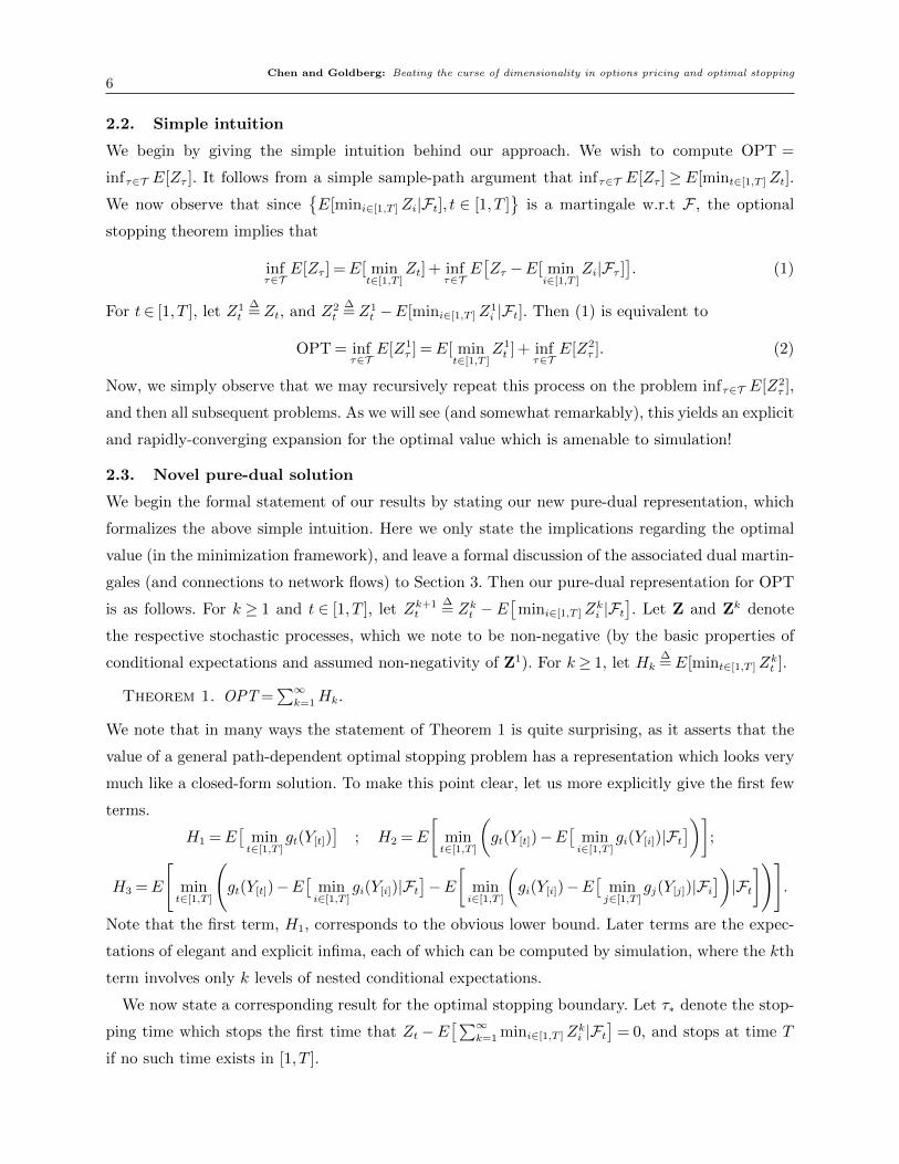
2.2. Simple intuition
We begin by giving the simple intuition behind our approach. We wish to compute OPT =
infτ∈T E[Zτ ]. It follows from a simple sample-path argument that infτ∈T E[Zτ ]≥ E[mint∈[1,T ]Zt].
We now observe that since{E[mini∈[1,T ]Zi|Ft], t ∈ [1, T ]
}is a martingale w.r.t F , the optional
stopping theorem implies that
infτ∈T
E[Zτ ] =E[ mint∈[1,T ]
Zt] + infτ∈T
E[Zτ −E[ min
i∈[1,T ]Zi|Fτ ]
]. (1)
For t∈ [1, T ], let Z1t
∆=Zt, and Z2
t
∆=Z1
t −E[mini∈[1,T ]Z1i |Ft]. Then (1) is equivalent to
OPT = infτ∈T
E[Z1τ ] =E[ min
t∈[1,T ]Z1t ] + inf
τ∈TE[Z2
τ ]. (2)
Now, we simply observe that we may recursively repeat this process on the problem infτ∈T E[Z2τ ],
and then all subsequent problems. As we will see (and somewhat remarkably), this yields an explicit
and rapidly-converging expansion for the optimal value which is amenable to simulation!
2.3. Novel pure-dual solution
We begin the formal statement of our results by stating our new pure-dual representation, which
formalizes the above simple intuition. Here we only state the implications regarding the optimal
value (in the minimization framework), and leave a formal discussion of the associated dual martin-
gales (and connections to network flows) to Section 3. Then our pure-dual representation for OPT
is as follows. For k ≥ 1 and t ∈ [1, T ], let Zk+1t
∆= Zkt −E
[mini∈[1,T ]Z
ki |Ft
]. Let Z and Zk denote
the respective stochastic processes, which we note to be non-negative (by the basic properties of
conditional expectations and assumed non-negativity of Z1). For k≥ 1, let Hk∆=E[mint∈[1,T ]Z
kt ].
Theorem 1. OPT =∑∞
k=1Hk.
We note that in many ways the statement of Theorem 1 is quite surprising, as it asserts that the
value of a general path-dependent optimal stopping problem has a representation which looks very
much like a closed-form solution. To make this point clear, let us more explicitly give the first few
terms.
H1 =E[
mint∈[1,T ]
gt(Y[t])]
; H2 =E
[mint∈[1,T ]
(gt(Y[t])−E
[mini∈[1,T ]
gi(Y[i])|Ft])]
;
H3 =E
[mint∈[1,T ]
(gt(Y[t])−E
[mini∈[1,T ]
gi(Y[i])|Ft]−E
[mini∈[1,T ]
(gi(Y[i])−E
[minj∈[1,T ]
gj(Y[j])|Fi])|Ft])]
.
Note that the first term, H1, corresponds to the obvious lower bound. Later terms are the expec-
tations of elegant and explicit infima, each of which can be computed by simulation, where the kth
term involves only k levels of nested conditional expectations.
We now state a corresponding result for the optimal stopping boundary. Let τ∗ denote the stop-
ping time which stops the first time that Zt−E[∑∞
k=1 mini∈[1,T ]Zki |Ft
]= 0, and stops at time T
if no such time exists in [1, T ].
Chen and Goldberg: Beating the curse of dimensionality in options pricing and optimal stopping7
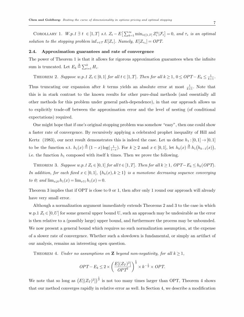
Corollary 1. W.p.1 ∃ t ∈ [1, T ] s.t. Zt−E[∑∞
k=1 mini∈[1,T ]Zki |Ft
]= 0, and τ∗ is an optimal
solution to the stopping problem infτ∈T E[Zτ ]. Namely, E[Zτ∗ ] = OPT.
2.4. Approximation guarantees and rate of convergence
The power of Theorem 1 is that it allows for rigorous approximation guarantees when the infinite
sum is truncated. Let Ek∆=∑k
i=1Hi.
Theorem 2. Suppose w.p.1 Zt ∈ [0,1] for all t∈ [1, T ]. Then for all k≥ 1, 0≤OPT−Ek ≤ 1k+1
.
Thus truncating our expansion after k terms yields an absolute error at most 1k+1
. Note that
this is in stark contrast to the known results for other pure-dual methods (and essentially all
other methods for this problem under general path-dependence), in that our approach allows us
to explicitly trade-off between the approximation error and the level of nesting (of conditional
expectations) required.
One might hope that if one’s original stopping problem was somehow “easy”, then one could show
a faster rate of convergence. By recursively applying a celebrated prophet inequality of Hill and
Kertz (1983), our next result demonstrates this is indeed the case. Let us define h1 : [0,1]→ [0,1]
to be the function s.t. h1(x)∆= (1− x) log( 1
1−x). For k ≥ 2 and x ∈ [0,1], let hk(x)∆= h1
(hk−1(x)
),
i.e. the function h1 composed with itself k times. Then we prove the following.
Theorem 3. Suppose w.p.1 Zt ∈ [0,1] for all t∈ [1, T ]. Then for all k≥ 1, OPT−Ek ≤ hk(OPT).
In addition, for each fixed x ∈ [0,1], {hk(x), k ≥ 1} is a monotone decreasing sequence converging
to 0; and limx↓0 h1(x) = limx↑1 h1(x) = 0.
Theorem 3 implies that if OPT is close to 0 or 1, then after only 1 round our approach will already
have very small error.
Although a normalization argument immediately extends Theorems 2 and 3 to the case in which
w.p.1 Zt ∈ [0,U ] for some general upper bound U, such an approach may be undesirable as the error
is then relative to a (possibly large) upper bound, and furthermore the process may be unbounded.
We now present a general bound which requires no such normalization assumption, at the expense
of a slower rate of convergence. Whether such a slowdown is fundamental, or simply an artifact of
our analysis, remains an interesting open question.
Theorem 4. Under no assumptions on Z beyond non-negativity, for all k≥ 1,
OPT−Ek ≤ 2×(E[(ZT )2]
OPT2
) 13
× k− 13 ×OPT.
We note that so long as(E[(ZT )2]
) 12 is not too many times larger than OPT, Theorem 4 shows
that our method converges rapidly in relative error as well. In Section 4, we describe a modification
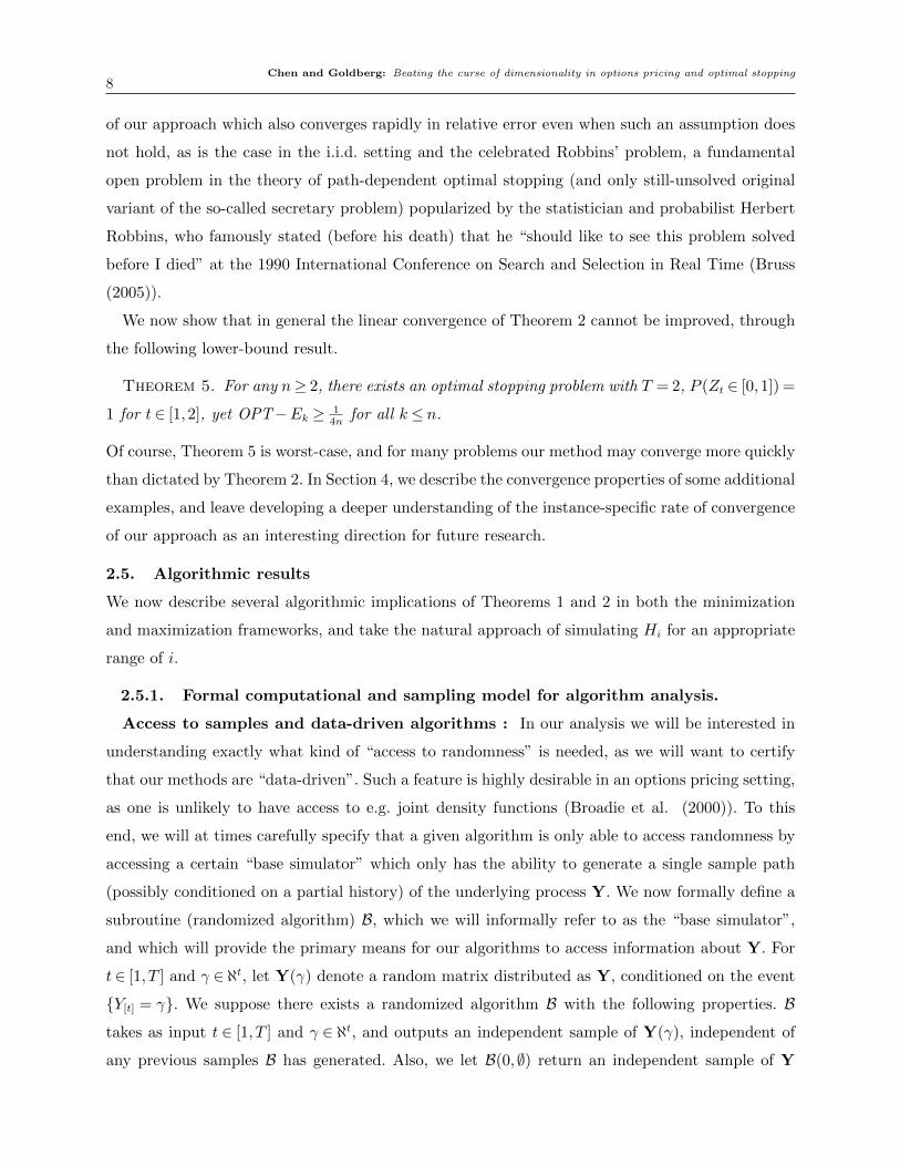
Chen and Goldberg: Beating the curse of dimensionality in options pricing and optimal stopping8
of our approach which also converges rapidly in relative error even when such an assumption does
not hold, as is the case in the i.i.d. setting and the celebrated Robbins’ problem, a fundamental
open problem in the theory of path-dependent optimal stopping (and only still-unsolved original
variant of the so-called secretary problem) popularized by the statistician and probabilist Herbert
Robbins, who famously stated (before his death) that he “should like to see this problem solved
before I died” at the 1990 International Conference on Search and Selection in Real Time (Bruss
(2005)).
We now show that in general the linear convergence of Theorem 2 cannot be improved, through
the following lower-bound result.
Theorem 5. For any n≥ 2, there exists an optimal stopping problem with T = 2, P (Zt ∈ [0,1]) =
1 for t∈ [1,2], yet OPT−Ek ≥ 14n
for all k≤ n.
Of course, Theorem 5 is worst-case, and for many problems our method may converge more quickly
than dictated by Theorem 2. In Section 4, we describe the convergence properties of some additional
examples, and leave developing a deeper understanding of the instance-specific rate of convergence
of our approach as an interesting direction for future research.
2.5. Algorithmic results
We now describe several algorithmic implications of Theorems 1 and 2 in both the minimization
and maximization frameworks, and take the natural approach of simulating Hi for an appropriate
range of i.
2.5.1. Formal computational and sampling model for algorithm analysis.
Access to samples and data-driven algorithms : In our analysis we will be interested in
understanding exactly what kind of “access to randomness” is needed, as we will want to certify
that our methods are “data-driven”. Such a feature is highly desirable in an options pricing setting,
as one is unlikely to have access to e.g. joint density functions (Broadie et al. (2000)). To this
end, we will at times carefully specify that a given algorithm is only able to access randomness by
accessing a certain “base simulator” which only has the ability to generate a single sample path
(possibly conditioned on a partial history) of the underlying process Y. We now formally define a
subroutine (randomized algorithm) B, which we will informally refer to as the “base simulator”,
and which will provide the primary means for our algorithms to access information about Y. For
t∈ [1, T ] and γ ∈ ℵt, let Y(γ) denote a random matrix distributed as Y, conditioned on the event
{Y[t] = γ}. We suppose there exists a randomized algorithm B with the following properties. B
takes as input t ∈ [1, T ] and γ ∈ ℵt, and outputs an independent sample of Y(γ), independent of
any previous samples B has generated. Also, we let B(0,∅) return an independent sample of Y
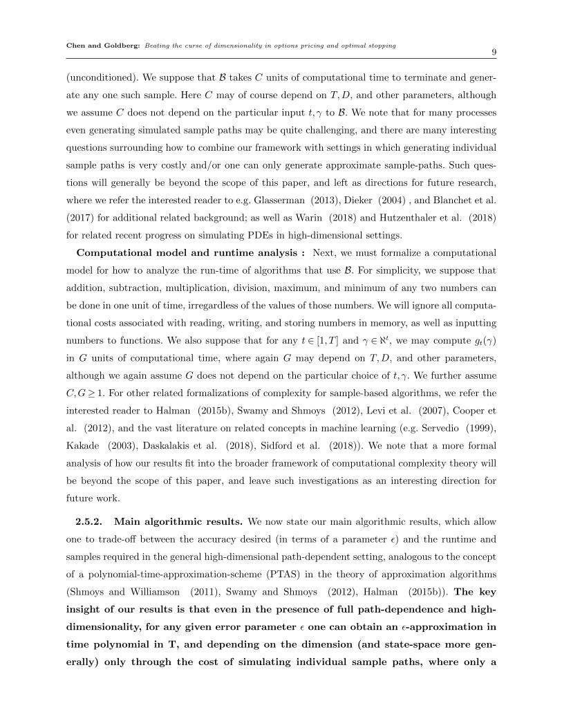
Chen and Goldberg: Beating the curse of dimensionality in options pricing and optimal stopping9
(unconditioned). We suppose that B takes C units of computational time to terminate and gener-
ate any one such sample. Here C may of course depend on T,D, and other parameters, although
we assume C does not depend on the particular input t, γ to B. We note that for many processes
even generating simulated sample paths may be quite challenging, and there are many interesting
questions surrounding how to combine our framework with settings in which generating individual
sample paths is very costly and/or one can only generate approximate sample-paths. Such ques-
tions will generally be beyond the scope of this paper, and left as directions for future research,
where we refer the interested reader to e.g. Glasserman (2013), Dieker (2004) , and Blanchet et al.
(2017) for additional related background; as well as Warin (2018) and Hutzenthaler et al. (2018)
for related recent progress on simulating PDEs in high-dimensional settings.
Computational model and runtime analysis : Next, we must formalize a computational
model for how to analyze the run-time of algorithms that use B. For simplicity, we suppose that
addition, subtraction, multiplication, division, maximum, and minimum of any two numbers can
be done in one unit of time, irregardless of the values of those numbers. We will ignore all computa-
tional costs associated with reading, writing, and storing numbers in memory, as well as inputting
numbers to functions. We also suppose that for any t ∈ [1, T ] and γ ∈ ℵt, we may compute gt(γ)
in G units of computational time, where again G may depend on T,D, and other parameters,
although we again assume G does not depend on the particular choice of t, γ. We further assume
C,G≥ 1. For other related formalizations of complexity for sample-based algorithms, we refer the
interested reader to Halman (2015b), Swamy and Shmoys (2012), Levi et al. (2007), Cooper et
al. (2012), and the vast literature on related concepts in machine learning (e.g. Servedio (1999),
Kakade (2003), Daskalakis et al. (2018), Sidford et al. (2018)). We note that a more formal
analysis of how our results fit into the broader framework of computational complexity theory will
be beyond the scope of this paper, and leave such investigations as an interesting direction for
future work.
2.5.2. Main algorithmic results. We now state our main algorithmic results, which allow
one to trade-off between the accuracy desired (in terms of a parameter ε) and the runtime and
samples required in the general high-dimensional path-dependent setting, analogous to the concept
of a polynomial-time-approximation-scheme (PTAS) in the theory of approximation algorithms
(Shmoys and Williamson (2011), Swamy and Shmoys (2012), Halman (2015b)). The key
insight of our results is that even in the presence of full path-dependence and high-
dimensionality, for any given error parameter ε one can obtain an ε-approximation in
time polynomial in T, and depending on the dimension (and state-space more gen-
erally) only through the cost of simulating individual sample paths, where only a
Chen and Goldberg: Beating the curse of dimensionality in options pricing and optimal stopping10
polynomial number of such simulations are needed. Furthermore, our methods are
data-driven, and require essentially no knowledge of any distributions beyond the
ability to generate samples. To our knowledge, these results are the first of their kind,
and act as a proof-of-concept that such a result is possible even in the path-dependent
and high-dimensional setting. We also note that our analysis and bounds are worst-case, and
in almost all cases we have opted for simplicity of analysis over tightness of bounds. Furthermore,
the fact that all relevant terms must actually be estimated by simulations, whose errors propagate
through our expansion, implies that our achieved runtime (although polynomial in T for any fixed
ε) will be considerably slower than the rate implied by Theorem 2. We leave providing a tighter
analysis and devising faster algorithms as interesting directions for future research, especially when
the underlying problem exhibits additional structure.
As noted before, to turn Theorems 1 and 2 into algorithms, we take the natural approach of
simulating Hi for an appropriate range of i. As suggested by Theorems 2 - 4, under different
assumptions on the relative scaling of various quantities (e.g. moments and upper bounds), one
may be able to prove different results as regards how many terms of the relevant series are needed
to achieve a given level of approximation. Furthermore, the precise notion of approximation is
similarly important, e.g. whether one is seeking absolute or relative error, and whether one is
content with error relative to an upper bound or e.g. E[(ZT )2]. These choices then dictate the
computational and sample complexity necessitated by our approach. We note that there are a vast
number of different settings one could consider along these lines, fine-tuning our approach and
deriving slightly different results under many different sets of assumptions. We make no attempt
to fully classify the associated tractability landscape here, leaving such an endeavor as an inter-
esting direction for future research. Instead, we focus on two illustrative settings. First, in the
minimization framework with the metric of absolute error, we consider the setting that Zt ∈ [0,1]
for all t∈ [1, T ], i.e. the normalized case. That setting is in a sense the most basic for our approach,
and illustrates most of the key ideas. We note that by applying a straightforward transformation,
all of our results for this normalized case (also w.r.t. implementing efficient stopping strategies)
carry-over essentially unchanged to the maximization setting, although for clarity of exposition we
do not formally state and prove such a transference. Second, in the maximization framework with
the metric of relative error, we consider a much more general setting : that in which all we assume
is that the squared coefficient of variation (i.e. ratio of the variance to the square of the mean) of
maxt∈[1,T ]Zt is nicely bounded and can be treated as a constant. For this second result, we note
that we do not require the process to be bounded or anything else, and note that such a modest
requirement on the associated coefficient of variation should hold in many settings of interest.
Chen and Goldberg: Beating the curse of dimensionality in options pricing and optimal stopping11
We note that our algorithms are constructed recursively, building a method for efficiently sim-
ulating Zk+1 out of one for efficiently simulating Zk, and that such nested schemes (albeit of a
different nature) have been considered previously in the literature (Kolodko et al. (2006)). For
k≥ 1 and ε, δ ∈ (0,1), let us define
fk(ε, δ)∆= 102(k−1)2 × ε−2(k−1)× (T + 2)k−1×
(1 + log(
1
δ) + log(
1
ε) + log(T )
)k−1.
We begin by stating our results in the minimization framework, for approximating OPT in absolute
error under the assumption that Z is normalized to lie in [0,1].
Theorem 6. Suppose w.p.1 Zt ∈ [0,1] for all t ∈ [1, T ]. Then for all k ≥ 1, there exists a ran-
domized algorithm Bk which takes as input any ε, δ ∈ (0,1), and achieves the following. In total
computational time at most (C + G + 1)fk+1(ε, δ), and with only access to randomness at most
fk+1(ε, δ) calls to the base simulator B, returns a random number X satisfying P(|X −Hk| ≤ ε
)≥
1− δ.
Combining Theorem 6 with Theorem 2 and a simple union bound, we are led to the following.
Corollary 2. Suppose w.p.1 Zt ∈ [0,1] for all t ∈ [1, T ]. Then there exists a randomized algo-
rithm A which takes as input any ε, δ ∈ (0,1), and achieves the following. In total computational
time at most
(C +G+ 1)exp(200ε−2)T 6ε−1(1 + log(
1
δ))6ε−1
,
and with only access to randomness at most
exp(200ε−2)T 6ε−1(1 + log(
1
δ))6ε−1
calls to the base simulator B, returns a random number X satisfying P(|X −OPT| ≤ ε
)≥ 1− δ.
Next, we state our results in the maximization framework, for approximating OPT in relative
error under the assumption that the squared coefficient of variation of maxt∈[1,T ]Zt can be treated
as a constant. We note that as in many other problems, here there seems to be an asymmetry
in the difficulty of approximation between the minimization and maximization frameworks, and
deriving equally general conditions under which one can derive efficient relative-error approximation
algorithms in the minimization framework remains an interesting direction for future research.
For simplicity in stating our results, algorithms, and analysis, in this setting we assume that
the input to our algorithm is not only ε and δ, but also the first two moments of maxt∈[1,T ]Zt.
Although these quantities can of course be estimated from data, e.g. using the base simulator,
incorporating this estimation into our algorithms introduces details and complexities tangential
to our main goals, and as such we simply assume these quantities have been estimated before

Chen and Goldberg: Beating the curse of dimensionality in options pricing and optimal stopping12
applying our algorithm. Again for clarity of exposition we assume exact knowledge of these two
moments, with the understanding that in many practical settings one would only have associated
(probabilistic) estimates, where we note that our algorithms could be easily modified to account
for such considerations, at the cost of slightly different guarantees and increased complexity in
describing our methods and results.
Theorem 7. Under no assumptions other than the non-negativity of Z and finiteness of M1∆=
E[maxt∈[1,T ]Zt],M2∆= E
[(maxt∈[1,T ]Zt
)2], the following is true. Let γ0
∆= M2
(M1)2, i.e. one plus the
squared coefficient of variation of the max. There exists a randomized algorithm A which takes as
input any ε, δ ∈ (0,1), and M1 =E[maxt∈[1,T ]Zt],M2 =E[(
maxt∈[1,T ]Zt)2]∈R+, and achieves the
following. In total computational time at most
(C +G+ 1)exp(1020γ9
0ε−6)T 108γ
920 ε−3(
1 + log(1
δ))108γ
920 ε−3
,
and with only access to randomness at most
exp(1020γ9
0ε−6)T 108γ
920 ε−3(
1 + log(1
δ))108γ
920 ε−3
calls to the base simulator B, returns a random number X satisfying P(|X − OPT| ≤ ε× OPT
)≥
1− δ.
Of course, for the explicit bounds of Theorem 6, Corollary 2, and Theorem 7, many known
methods will (for many parameter regimes) exhibit much faster runtimes. However, we emphasize
that essentially all of the aforementioned ADP methods have runtimes which scale exponentially
in the dimension (also typically requiring a Markovian assumption), and all of the aforementioned
iterative or pure-dual methods have runtimes which scale exponentially in the time horizon, if one
requires theoretical guarantees of good performance. Indeed, the existence of an algorithm which
can yield a solution with strong theoretical approximation guarantees in time polynomial in both
the dimension and time horizon was not previously known to exist. We leave as a pressing direction
for future research devising tighter bounds and more practical algorithms, based on the insights
from this work, and also understanding which methods may be best for which parameter settings
and instance-specific features. We also note that although such polynomial bounds were not known
for any existing methods, it is also an interesting question whether (especially in light of our own
work) such bounds can be proven, perhaps for suitable modifications of those methods.
We next state our algorithmic results w.r.t. implementing efficient stopping strategies with anal-
ogous performance guarantees. For space considerations and clarity of exposition, we only state
such results in the minimization framework under our previous normalization assumption, and
again note that analogous results may be proven under a variety of different assumptions. There is
Chen and Goldberg: Beating the curse of dimensionality in options pricing and optimal stopping13
a subtlety here, as one might think that since our previous results yield approximate value-function
evaluations, it should be immediate from known black-box reductions (Singh and Yee (1994)) that
we also get a good approximate stopping strategy. However, the problem with such an approach
is it would typically require one to approximate the value function to an additive error going to
0 as T grows large (Singh and Yee (1994), Chen and Glasserman (2007), Van Roy (2010)). In
our framework, this would not work, as it would require deeply nested conditional expectations.
Fortunately, en route to our main results we will prove strong pathwise convergence results, which
will allow us to overcome this problem, yielding the following results. We note that our results are
stated in terms of the existence of an efficiently implementable randomized stopping time, and we
refer the reader to Chalasani et al. (2001) and Levin and Peres (2017) for associated standard
definitions regarding the formal definition of a randomized stopping time as an appropriate mix-
ture of F-adapted stopping times. We also note that several past works have explicitly studied
the connection between value-function-approximation and approximately optimal stopping times
in the context of optimal stopping and options pricing, but their results are incomparable to our
own (Van Roy (2010), Belomestny (2011)).
Corollary 3. Suppose w.p.1 Zt ∈ [0,1] for all t ∈ [1, T ]. Then for all ε ∈ (0,1), there exists
a randomized stopping time τε s.t. E[Zτε ]−OPT ≤ ε, and with the following properties. At each
time step, the decision of whether to stop (if one has not yet stopped) can be implemented in total
computational time at most (C +G+ 1)fd 4ε e(ε4, ε
4T) , and with only access to randomness at most
fd 4ε e(ε4, ε
4T) calls to the base simulator B.
Although we defer the details of the stopping time τε and all relevant algorithms to Section 5, we
note that intuitively one can (roughly) take τε to be the stopping time which stops the first time
that (a simulated approximation of) Zd 4ε et is less than 1
2ε.
We conclude this section by briefly circling back to our statement in Section 1 regarding the fact
that the problem supτ∈T E[Zτ ], the setting of primary interest in the context of options pricing,
can w.l.o.g. be transformed into a problem of the form infτ∈T E[Z ′τ ] for appropriate non-negative
Z ′. Of course, if there exists a finite known upper bound U on Z, one can set Z ′t = U − Zt, in
which case supτ∈T E[Zτ ] =U− infτ∈T E[Z ′τ ]. Alternatively, if such an upper bound is unavailable or
computationally undesirable, one can set Z ′t =E[maxi∈[1,T ]Zi|Ft]−Zt, in which case (by optional
stopping) supτ∈T E[Zτ ] =E[maxt∈[1,T ]Zt]− infτ∈T E[Z ′τ ]. Under both transformations, one can then
apply our approach to the associated minimization problem, where we note that all relevant run-
time analyses remain unchanged in their essential parts with only minor modification, e.g. under
the second transformation all recursions must be carried out to one greater depth as even Z ′t
must be computed by estimating an appropriate conditional expectation. Indeed, our results in
the maximization framework, i.e. Theorem 7, implement such a transformation combined with a
carefully chosen truncation.
Chen and Goldberg: Beating the curse of dimensionality in options pricing and optimal stopping14
2.6. Outline of rest of paper
The remainder of the paper proceeds as follows. We derive our pure-dual martingale representa-
tion, compare to related approaches from the literature, and give an interpretation in terms of
network flows in Section 3. In Section 4 we prove several bounds on the rate of convergence of our
methodology, and provide several illustrative examples. We derive our main algorithmic results in
Section 5, proving explicit bounds on the required computational and sample complexity needed
to achieve a given performance guarantee. We provide concluding remarks and some interesting
directions for future research in Section 6. We also provide a technical appendix in Section 7, which
contains several proofs from throughout the paper.
3. Proof of Theorem 1, dual martingales, and network flows.
In this section we formalize our pure-dual approach and prove Theorem 1, put our results in the
broader context of other related work, and give a formulation in terms of network flows.
3.1. Proof of Theorem 1
We begin by observing that our earlier simple intuition from Section 2.2, i.e. recursively apply-
ing the optional stopping theorem to the appropriate remainder term, combined with definitions,
immediately yields the following.
Lemma 1. For all k ≥ 1, OPT =∑k
i=1E[mint∈[1,T ]Zit ] + infτ∈T E[Zk+1
τ ]. In addition, w.p.1 Zkt
is non-negative for all k≥ 1 and t∈ [1, T ]; and for each t∈ [1, T ], w.p.1 {Zkt , k≥ 1} is a monotone
decreasing sequence of random variables.
We would be done (at least with the proof of Theorem 1) if we could show that
limk→∞ infτ∈T E[Zk+1τ ] = 0. We now prove this, thus completing the proof of Theorem 1.
Proof of Theorem 1: It follows from monotone convergence that {Zk, k≥ 1} converges a.s., and
thus {Zk+1T −ZkT , k ≥ 1} converges a.s. to 0. Since by definition, for all k ≥ 1, w.p.1 Zk+1
T = ZkT −
E[mini∈[1,T ]Z
ki |FT
], and by measurability w.p.1 E
[mini∈[1,T ]Z
ki |FT
]= mini∈[1,T ]Z
ki , we conclude
that
{ mini∈[1,T ]
Zki , k≥ 1} converges a.s. to 0. (3)
Thus, for any j ≥ 1, there exists Kj s.t. k ≥Kj implies P(
mini∈[1,T ]Zki ≥ 1
j
)< 1
j2. It follows that
there exists a strictly increasing sequence of integers {K ′j, j ≥ 1} s.t. P(
mini∈[1,T ]ZK′ji ≥ 1
j
)< 1
j2.
For stopping problem infτ∈T E[ZK′jτ ], consider the stopping time τ ′j which stops the first time
ZK′jt ≤ 1
j, and stops at time T if no such time has yet occurred by the end of the horizon. Let I ′j
be the indicator for the event{
mini∈[1,T ]ZK′ji > 1
j
}. Note that w.p.1, Z
K′jτ ′j≤Zj
∆= 1
j+ I ′jZ
K′jT . Recall
that under our definitions, {ZK′j , j ≥ 1} are all constructed on the same probability space, and thus
{ZK′j
T , j ≥ 1} is monotone decreasing. It follows from Borel-Cantelli that {I ′j, j ≥ 1} equals 0 after
Chen and Goldberg: Beating the curse of dimensionality in options pricing and optimal stopping15
some a.s. finite time, and thus {Zj, j ≥ 1} converges a.s. to 0. But by monotonicity, integrabil-
ity, and non-negativity, we may apply dominated convergence to conclude that limj→∞E[Zj] = 0,
which implies that limj→∞E[ZK′jτ ′j
]= 0, and thus limj→∞ infτ∈T E[Z
K′jτ ] = 0. Thus the sequence
{infτ∈T E[Zjτ ], j ≥ 1}, which is monotone decreasing by non-negativity and Lemma 1, has a subse-
quence which converges to 0, and thus must itself converge to 0. Letting k→∞ in Lemma 1 then
completes the proof. Q.E.D.
3.2. The optimal dual martingale and Proof of Corollary 1
We now explicitly describe the optimal martingale derived from our approach. First, we provide
some additional background on martingale duality.
3.2.1. Background on martingale duality. There are many different, essentially equivalent
statements of the relevant duality, and we take as our starting point a formulation essentially iden-
tical to what is referred to in several papers as a dual satisfying 0-sure-optimality (Schoenmakers
et al. (2013), Belomestny et al. (2013), Belomestny (2017)).
Lemma 2 (0-sure-optimal dual for optimal stopping).
OPT = sup
{x∈R : ∃ M ∈Mx s.t. P
(mint∈[1,T ]
(Z1t −Mt
)= 0
)= 1
}.
We note that prior works studying 0-sure-optimal martingale duality actually imply that any
martingale M adapted to F s.t. P(
mint∈[1,T ]
(Z1t −Mt
)= 0)
= 1 must have mean equal to OPT, but
for our purposes an optimization-oriented formulation as asserted in Lemma 2 will be convenient.
3.2.2. Our optimal dual martingale. Let S∆=∑∞
k=1 mini∈[1,T ]Zki , where we note that S is
non-negative with finite mean by Theorem 1 and monotone convergence. Let MAR denote the
Doob martingale s.t. MARt = E[S|Ft
], t ∈ [1, T ]. We now prove that MAR is the optimal dual
martingale arising from our pure-dual approach. Recall from Lemma 1 (and monotone convergence)
that {Zk, k≥ 1} converges a.s. to a limiting T-dimensional random vector Z∞ = {Z∞t , t∈ [1, T ]}.
Lemma 3. E[MAR1] = OPT, and P
(mint∈[1,T ]
(Z1t −MARt
)= 0
)= 1.
Proof: For all t∈ [1, T ], Z1t −MARt equals
Z1t −E
[ ∞∑k=1
mini∈[1,T ]
Zki |Ft]
= Z1t −E[ min
i∈[1,T ]Z1i |Ft]−E
[ ∞∑k=2
mini∈[1,T ]
Zki |Ft]
= Z2t −E
[ ∞∑k=2
mini∈[1,T ]
Zki |Ft].
By applying the above inductively, we find that for all j ≥ 1 and t∈ [1, T ], w.p.1
Z1t −MARt =Zjt −E
[ ∞∑k=j
mini∈[1,T ]
Zki |Ft]. (4)
Chen and Goldberg: Beating the curse of dimensionality in options pricing and optimal stopping16
By taking limits in (4), we now prove that w.p.1
Z1t −MARt =Z∞t for all t∈ [1, T ]. (5)
Indeed, we already know that {Zjt , j ≥ 1} converges a.s. to Z∞t for all t∈ [1, T ]. Next, we claim that{E[∑∞
k=j mini∈[1,T ]Zki |Ft
], j ≥ 1
}converges a.s. to 0 for all t∈ [1, T ]. Since
{∑∞k=j mini∈[1,T ]Z
ki , j ≥
1}
is monotone and non-negative, and conditional expectation preserves almost sure dominance,
it follows that{E[∑∞
k=j mini∈[1,T ]Zki |Ft
], j ≥ 1
}is monotone and non-negative. Hence by mono-
tone convergence,{E[∑∞
k=j mini∈[1,T ]Zki |Ft
], j ≥ 1
}converges almost surely to a limiting non-
negative r.v. Qt, and E[Qt] = limj→∞E[∑∞
k=j mini∈[1,T ]Zki
]. Combining with Theorem 1, we
conclude that E[Qt] = 0, and thus by non-negativity Qt = 0 w.p.1, completing the proof that{E[∑∞
k=j mini∈[1,T ]Zki |Ft
], j ≥ 1
}converges a.s. to 0 for all t∈ [1, T ].
Taking limits (in j) in the right-hand-side of (4) then completes the proof of (5). Next, note
that the basic properties of a.s. convergence, continuity of the min function, and a.s. conver-
gence of {Zk, k ≥ 1} to Z∞, imply that {mini∈[1,T ]Zki , k ≥ 1} converges a.s. to mini∈[1,T ]Z
∞i .
Combining with (3), we conclude that mini∈[1,T ]Z∞i = 0 w.p.1. Combining the above, it follows
that P
(mint∈[1,T ]
(Z1t −MARt
)= 0
)= 1. As Theorem 1 and the definition of MAR imply that
E[MAR1] = OPT, this completes the proof. Q.E.D.
3.2.3. Proof of Corollary 1.
Proof of Corollary 1 : The proof follows immediately from Lemmas 3 and 2, combined with
optional stopping, and we omit the details. Q.E.D.
3.3. Optimization formulations for duality, non-negativity, and network flows
In this section we describe a novel connection between optimal stopping and max-flow problems.
For an overview of max-flow problems and network optimization more generally, we refer the reader
to Ahuja et al. (2014) and Christiano et al. (2011). Linear programming (LP) formulations for
optimal stopping have been studied by several authors, and we refer the reader to the very relevant
work Chen and Glasserman (2007), which connects LP duality to martingale duality, as well as
other works such as Buchbinder et al. (2010). However, it seems that previous authors never
made the leap from such LPs to even more structured max-flow problems. We do note that some
relevant considerations of non-negativity were previously studied for the multiplicative form of the
martingale dual in Jamshidian (2007), although no connection to max-flow was made.
3.3.1. Additional notations. For simplicity, we suppose (in this section only) that there is
a finite (possibly very large) set S of D-dimensional vectors s.t. for all t ∈ [1, T ], and all D by t
matrices γ one can form by drawing all columns from S (in an arbitrary manner, possibly with
repetition), it holds that P (Y[t] = γ) > 0, while P (Y[t] = γ′) = 0 for any γ′ ∈ ℵt which cannot be
Chen and Goldberg: Beating the curse of dimensionality in options pricing and optimal stopping17
formed in this way. Letting ℵt denote the set of all D by t matrices γ one can form by drawing
all columns from S, this is equivalent to assuming P (Y[t] ∈ ℵt) = 1, and P (Y[t] = γ) > 0 for all
γ ∈ ℵt. Note that our assumption further implies that for all t ∈ [1, T − 1], v ∈ S, and γ ∈ ℵt,
P (Yt+1 = v|Y[t] = γ)> 0. Of course, these probabilities may be very different for different t, γ, s. We
further assume that all v ∈ S have rational entries, and that P (Y[t] = γ) is rational for all t∈ [1, T ]
and γ ∈ ℵt, to preclude certain pathologies when talking about flows. These conditions, although
not strictly necessary, will simplify notations considerably. Furthermore, it follows from standard
approximation arguments that these assumptions are essentially w.l.o.g. For any martingale M
adapted to F , any t ∈ [1, T ], and any γ ∈ ℵt, let Mt(γ) denote the value of the martingale at
time t when Y[t] = γ. For t ∈ [1, T − 1], γ ∈ ℵt, and v ∈ S, let γ|v denote the element of ℵt+1s.t.
γ|v[t] = γ, γ|vt+1 = v, i.e. the matrix derived by appending v to the right of γ.
3.3.2. Optimization formulations and non-negativity. We begin by observing that the
dual characterization for OPT given in Lemma 2 can be formulated as an optimization problem as
follows. This follows from the basic definitions associated with martingales, and is generally known
(Chen and Glasserman (2007)).
Lemma 4. OPT is equivalent to the value of the following optimization problem OPT1, with
variables {Mt(γ), t∈ [1, T ], γ ∈ ℵt}.
max∑
v∈SM1(v)P (Y1 = v)
Mt(γ) =∑
v∈SMt+1(γ|v)P(Yt+1 = v|Y[t] = γ
)for all t∈ [1, T − 1], γ ∈ ℵt;
Mt(γ)≤Zt(γ) for all t∈ [1, T ], γ ∈ ℵt;
For all γ ∈ ℵT , there exists t∈ [1, T ] s.t. Mt(γ[t]) =Zt(γ[t]).
However, what we believe prior works failed to do was fully utilize the fact that OPT1 has an
optimal solution which is non-negative, where we note that most dual martingale solutions pro-
posed previously in the literature would not necessarily be non-negative. Indeed, it follows from
Lemma 3 that OPT1 has a non-negative optimal solution. Imposing such non-negativity, combining
with a straightforward contradiction argument which then allows us to drop the final constraint
(which is always binding in the optimal solution to any max-flow problem), and performing the
transformation Ft(γ) =Mt(γ)P (Y[t] = γ), we arrive at the following reformulation.
Lemma 5. OPT is equivalent to the value of the following linear program LP2, with variables
{Ft(γ), t∈ [1, T ], γ ∈ ℵt}.
max∑
v∈S F1(v)
Ft(γ) =∑
v∈S Ft+1(γ|v) for all t∈ [1, T − 1], γ ∈ ℵt;
0≤ Ft(γ)≤Zt(γ)P (Y[t] = γ) for all t∈ [1, T ], γ ∈ ℵt.
Chen and Goldberg: Beating the curse of dimensionality in options pricing and optimal stopping18
3.3.3. Connection to max-flow min-cut. We now observe that LP2 is a standard max s-t
flow problem. Indeed, consider a flow network N with source node s and sink node t, constructed
as follows. For all i∈ [1, T ] and γ ∈ ℵi, there is a node nγ , in addition to the source node s and sink
node t. For all γ ∈ ℵ1, there is an undirected edge (s,nγ), i.e. between node s and node nγ , with
capacity Z1(γ)P (Y[1] = γ). For all γ ∈ ℵT , there is an undirected edge (nγ , t) with capacity∞. For all
i ∈ [1, T − 1], γ ∈ ℵi, v ∈ S, there is an undirected edge (nγ , nγ|v) with capacity Zi+1(γ|v)P (Y[i+1] =
γ|v). Then standard arguments from max-flow theory (the details of which we omit) yield the
following.
Lemma 6. OPT is equivalent to the value of a maximum s-t flow in network N. Using the relation
Ft(γ) =Mt(γ)P (Y[t] = γ), one may recover a 0-sure-optimal dual martingale from an optimal flow
in network N, and visa-versa.
Interestingly, max-flow min-cut then reveals a very natural interpretation of optimal stopping in
terms of finding the minimum cut in N, where we note that there is indeed a straightforward
bijection between minimal cuts in N and stopping times. Although a closely related observation
was made in Chen and Glasserman (2007), it seems this explicit connection between optimal
stopping and max-flow / min-cut is novel. We leave further exploring this connection, e.g. applying
other algorithms from the well-established theory of max-flows to optimal stopping and options
pricing, as an interesting direction for future research. In addition, we note that optimal stopping
and options pricing thus provide another simple yet elegant testament to the power of network
flows as a modeling tool and optimization framework.
N’s special structure endows the underlying max-flow problem with some special features, which
may be helpful in devising other flow-inspired algorithms for optimal stopping. We note that there
is a vast literature on specialized algorithms for related families of networks (Brucker (1984),
Hoffman (1988), Goldberg and Tarjan (1988), Hoffman (1992), Vishkin (1992), Cohen (1995)).
For example, let us recall that in an s-t flow problem, a blocking flow is a feasible flow such
that every s-t path has at least one saturated edge, i.e. edge whose flow equals the capacity of
that edge. It is well-known that in a general max s-t flow problem, a blocking flow need not be
optimal, although any optimal flow must be a blocking flow. However, in a tree network such as
N, it is actually true that every blocking flow is optimal. The proof follows from a straightforward
contradiction argument and is generally well-known, and we omit the details (Hoffman (1985,
1992)). This fact provides a different way to interpret several properties of 0-sure-optimal dual
martingales which appear in previous works, which all boil down to the fact that if a certain process
has a zero along every sample path then a certain martingale must be dual-optimal.
As max-flow is already a polynomial-time solvable problem, and the max-flow problem on N

Chen and Goldberg: Beating the curse of dimensionality in options pricing and optimal stopping19
is even easier due to its tree structure (and can in fact be solved by a simple dynamic program
which is conceptually equivalent to the backwards-induction approach to optimal stopping), one
can of course ask why path-dependent optimal stopping should be considered a hard problem.
The answer is that even very fast max-flow algorithms typically focus on a runtime polynomial in
the number of nodes and edges, which will grow exponentially in T for path-dependent optimal
stopping. Our pure-dual representation and Theorem 1 can be interpreted as an algorithm for
such flow problems, which augments flow along all paths simultaneously in a series of rounds (each
term of our expansion corresponding to the total flow pushed in a given round). For example,
in the first round, the amount of flow pushed along the s-t path corresponding to γ ∈ ℵT equals(mint∈[1,T ]Zt(γ[t])
)×P (Y[T ] = γ), and hence the total flow pushed in the first round (by summing
over all paths) equals E[mint∈[1,T ]Zt]. Similarly, for t∈ [1, T −1], γ ∈ ℵt, and v ∈ S, the flow pushed
along the edge (nγ , nγ|v) in the first round equals E[mini∈[1,T ]Zi
∣∣Ft+1
](γ|v)×P
(Yt+1 = γ|v
), where
we note that feasibility (w.r.t. capacities) follows from the fact that E[mini∈[1,T ]Zi
∣∣Ft+1
](γ|v)≤
Zt+1(γ|v). Theorem 2 bounds the distance from optimality after a given number of such rounds,
while our algorithmic results can be interpreted as providing a very fast randomized algorithm for
estimating the amount of flow pushed in each round (and hence the optimal value itself).
3.4. Sure-optimal dual and algorithmic speedup
In this section we comment on a stronger sense in which certain dual martingales may be optimal,
note that our approach does not have this property, and conjecture that this may play an important
role in allowing our method to yield approximate solutions so quickly. For 1≤ t1 ≤ t2 ≤ T , let T t1,t2
denote the set of all integer-valued stopping times τ , adapted to F , s.t. w.p.1 t1 ≤ τ ≤ t2. Let us say
that M ∈M0 has the sure-optimal property (w.r.t. Z) if: 1. P
(mint∈[1,T ]
(Zt−Mt
)= OPT
)= 1;
and 2. for all i ∈ [1, T ], P
(mint∈[i,T ]
(Zt−Mt +Mi
)= infτ∈T i,T E[Zτ |Fi]
)= 1. We note that here
we refer only to 0-mean martingales, as it simplifies the relevant discussions (and is w.l.o.g by
appropriate translations and known results). As argued in Schoenmakers et al. (2013), every
optimal stopping problem has such a sure-optimal dual solution, and this property may be helpful
in algorithm design as it yields an optimality characterization in terms of certain suprema having
zero variance. Schoenmakers et al. (2013) also notes that there are some dual approaches which
yield 0-sure-optimal martingales, but not sure-optimal martingales, although most approaches
indeed yield sure-optimal dual solutions. Interestingly, our approach does not necessarily yield a
sure-optimal martingale, as we now show through a simple example, where we defer all associated
proofs to the technical appendix.
Consider the setting in which the dimension D = 1, the horizon T = 3; Y1 = 0 w.p.1; Y2 = 1
w.p.1; Y3 equals 12
w.p. 12, and equals 1 w.p. 1
2; and the stopping problem is simply infτ∈T E[Yτ ],
i.e. gt(Y[t]) = Yt for all t∈ [1,3].

Chen and Goldberg: Beating the curse of dimensionality in options pricing and optimal stopping20
Lemma 7. In this setting, the unique (0-mean) surely-optimal dual martingale M satisfies
M1(0) =M2(0,1) = 0,M3(0,1,1) = 14,M3(0,1, 1
2) =− 1
4. It follows that P (M1 = 0) = P (M2 = 0) = 1,
while P (M3 = 14) = P (M3 = − 1
4) = 1
2. However, the optimal dual martingale MAR derived from
our approach satisfies P (MARt = 0) = 1 for all t.
We suspect that the lack of sure-optimality may be fundamental in allowing our method to yield
quick approximations. Intuitively, any method which yields a sure-optimal dual martingale must
(in some sense) be solving all of the subproblems defined on all the subtrees of N. Our method of
approximation is fast precisely because it does not have to do this. We leave formalizing this line
of reasoning, and understanding associated lower bounds and the connection of our approach to
other dual formulations in general, as an interesting direction for future research.
4. Rate of convergence and Proofs of Theorems 2 - 5
In this section we prove Theorems 2 - 5, our main results regarding rate of convergence. Along
the way, we prove a much stronger path-wise convergence result, which will later enable us to
construct provably good approximate policies, beyond the standard framework of approximate
value functions. We also prove that a slight modification of our approach converges rapidly in
relative error, even when(E[(ZT )2]
) 12 is much larger than OPT, and apply these results to several
problems of interest in the optimal stopping literature - the i.i.d. setting and Robbins’ problem.
Finally, we provide several additional examples illustrating that our approach may converge much
more quickly for certain instances.
4.1. Proof of Theorem 2
In this section we prove our main rate of convergence result Theorem 2. First, we prove a much
stronger path-wise convergence result, essentially that after k iterations of our expansion, the
minimum of every sample path is at most 1k+1
. This is a much stronger statement than that given in
Theorem 2, which only regards expectations. We begin by proving the following strong convergence
result, whose proof is surprisingly simple.
Lemma 8. Suppose w.p.1 Zt ∈ [0,U ] for all t∈ [1, T ]. Then for all k≥ 1, w.p.1 mint∈[1,T ]Zkt ≤ U
k.
Proof : Note that by definitions, measurability, and Lemma 1, for all k ≥ 1, Zk+1T = ZT −∑k
i=1 mint∈[1,T ]Zit ≥ 0 w.p.1. By the monotonicity ensured by Lemma 1, it follows that w.p.1,
k×mint∈[1,T ]Zkt ≤ZT ≤U , and the desired result follows. Q.E.D.
Proof of Theorem 2 : By Lemma 1, OPT =∑k
i=1E[mint∈[1,T ]Zit ] + infτ∈T E[Zk+1
τ ]. Letting
τk+1 denote the stopping time which stops the first time Zk+1t ≤ 1
k+1(and stops at time T if no
such time exists), Lemma 8 implies that E[Zk+1τk+1
]≤ 1k+1
. It follows that infτ∈T E[Zk+1τ ]≤ 1
k+1, and
combining the above completes the proof. Q.E.D.

Chen and Goldberg: Beating the curse of dimensionality in options pricing and optimal stopping21
4.2. Alternate bounds with prophet inequalities and Proof of Theorem 3
Some of the most celebrated results in optimal stopping involve the so-called prophet inequalities,
relating infτ∈T E[Zτ ] to E[mint∈[1,T ]Zt] under various assumptions on Z, including boundedness,
independence, etc. We make no attempt to survey the vast literature on such inequalities here,
instead referring the reader to the classical survey of Hill and Kertz (1992), and the more recent
survey (with a more economics-oriented perspective) of Lucier (2017). We note that many of
these results in the literature hold only under an independence assumption, which will not be well-
suited to our purposes, as even if {Zt, t ∈ [1, T ]} is i.i.d., {Z2t , t ∈ [1, T ]} will in general not be so.
However, there are some notable exceptions, including the following result of Hill and Kertz (1983).
Although originally stated in terms of maximization, we here state the corresponding version for
minimization, which is easily derived from the original result of Hill and Kertz (1983), and we
omit the details. Recall that for x ∈ [0,1], h1(x) = (1− x) log( 11−x); and for k ≥ 2 and x ∈ [0,1],
hk(x) = h1
(hk−1(x)
).
Lemma 9 (Prophet inequality for bounded sequences (Hill and Kertz (1983))).
Suppose P(Zt ∈ [0,1]
)= 1 for all t∈ [1, T ]. Then OPT−E[mint∈[1,T ]Zt]≤ h1(OPT).
4.2.1. Proof of Theorem 3.
Proof of Theorem 3 : We begin by stating some basic properties of h1 which are easily verified
by straightforward calculus arguments, and we omit the details. First, h1(x)∈ [0,1] for all x∈ [0,1].
Second, h1(x)≤ x for all x ∈ [0,1], from which it follows by a straightforward induction argument
that for each fixed x∈ [0,1], {hk(x), k≥ 1} is monotone decreasing. Third, h1 is strictly increasing
on [0,1− exp(−1)]. Fourth, h1(x)≤ exp(−1) for all x∈ [0,1].
Next, we prove that for all k≥ 1, OPT−Ek ≤ hk(OPT), and proceed by induction. Since Lemma
1 implies that OPT =Ek + infτ∈T E[Zk+1τ ] for all k≥ 1, the desired result is equivalent to proving
that, for all k ≥ 1, infτ∈T E[Zk+1τ ] ≤ hk
(OPT
). The base case k = 1 follows immediately from
Lemma 1 and Lemma 9. Now, let us proceed by induction. Suppose the desired statement is true
for some k ≥ 1. Then from definitions, optional stopping, and Lemma 9, infτ∈T E[Zk+2τ ] equals
infτ∈T E[Zk+1τ −E[mint∈[1,T ]Z
k+1t |Fτ ]
], itself equal to
infτ∈T
E[Zk+1τ ]−E[ min
t∈[1,T ]Zk+1t ] ≤ h1
(infτ∈T
E[Zk+1τ ]
).
By our induction hypothesis, infτ∈T E[Zk+1τ ] ≤ hk
(OPT
). As we have already shown that
hk(OPT
)≤ h1
(OPT
)≤ exp(−1) < 1− exp(−1), and that h1 is increasing on [0,1− exp(−1)], it
follows that
h1
(infτ∈T
E[Zk+1τ ]
)≤ h1
(hk(OPT
))= hk+1(OPT).
Combining the above completes the induction, and further combining with some straightforward
algebra completes the proof of the theorem. Q.E.D.

Chen and Goldberg: Beating the curse of dimensionality in options pricing and optimal stopping22
We note that unfortunately, it can be shown that hk(x) does not in general (i.e. if one takes
the worst-case over all x ∈ [0,1]) yield a better bound than Theorem 2 as k→∞. However, it
may yield strong bounds for particular values of OPT. For example, if OPT is close to 1, then
Theorem 3 implies that our approach has small error after even a single iteration. More generally,
Lemma 9 can also be used to prove alternative bounds on both OPT−Ek and how much progress
is made during the kth iteration of our expansion, e.g. by using the fact (which follows from a
straightforward Taylor expansion) that h1(x)∼ x− x2
2as x ↓ 0, although we do not pursue such an
analysis here.
4.3. Alternate bounds when Z is unbounded and Proof of Theorem 4
We now complete the proof of Theorem 4, which provides a bound on the rate of convergence
which is completely general, i.e. neither requiring normalization, nor rescaling of the absolute error
by any upper bound, nor even the existence of any upper bound.
Proof of Theorem 4 : First, we claim that for all k≥ 1,
E[ mint∈[1,T ]
Zkt ]≤ 1
k×OPT. (6)
Indeed, this follows directly from monotonicity and Lemma 1, which also implies (by some straight-
forward algebra) that to prove the overall theorem, it suffices to prove that
infτ∈T
E[Zk+1τ ]≤ 2×
(OPT×E[(ZT )2]
) 13 × 1
k13
. (7)
To proceed, let us consider the performance of the following threshold policy. Let xk∆=(E[(ZT )2]×
OPT× k−1) 1
3 . Consider the policy which stops the first time that Zk+1t ≤ xk, and simply stops
at time T if no such t exists in [1, T ]. Denoting this stopping time by τk, note that w.p.1 Zk+1τk≤
xk + I(
mint∈[1,T ]Zk+1t > xk
)Zk+1T , which by monotonicity (implying Zk+1
T ≤ ZT w.p.1) is at most
xk + I(
mint∈[1,T ]Zk+1t > xk
)ZT . Taking expectations and applying Cauchy-Schwarz, we find that
E[Zk+1τk
] is at most xk +(E[(ZT )2]
) 12 ×
(P(
mint∈[1,T ]Zk+1t > xk
)) 12
. Further applying Markov’s
inequality and (6), we conclude that E[Zk+1τk
] is at most xk+(
OPT×k−1×E[(ZT )2]
xk
) 12 = 2xk, completing
the proof. Q.E.D.
4.4. Alternate bounds for the i.i.d. setting and Robbins’ problem
In some cases, it may be desirable to have guarantees not just on the absolute error, but on
the relative error. Namely, one might hope that after a few rounds, the error is at most a small
fraction of OPT itself. Theorem 4 yields such a result so long as(E[(ZT )2]
) 12 is not too many times
larger than OPT. However, many particular theoretical stopping problems studied intensely in the
literature, e.g. the setting in which Z is i.i.d. from a uniform distribution on [0,1] (i.e. U[0,1]), or the
Chen and Goldberg: Beating the curse of dimensionality in options pricing and optimal stopping23
celebrated Robbins’ problem (Bruss (2005)), have the feature that when T is large,(E[(ZT )2]
) 12
is many times larger than OPT. In such a setting, the bounds of Theorems 2 - 4 may require k to
be very large (scaling with T ) before achieving small relative error.
We now show that a small modification of our approach can overcome this. We note that although
we suspect that our approach, unmodified, also achieves good performance w.r.t. relative error
for such problems (not captured by our proven bounds), we leave this as an interesting open
question. Let Y1 = {Y 1i , i ≥ 1} denote an i.i.d. sequence of U[0,1] r.v.s. For T ≥ 1 and t ∈ [1, T ],
let gUt (Y 1[t])
∆= Y 1
t ; and gRt (Y 1[t])
∆=∑t
i=1 I(Y 1i ≤ Y 1
t ) + (T − t)Y 1t . Then it is easily verified that the
problem of optimal stopping for an i.i.d. U[0,1] sequence of r.v.s is equivalent to the problem
OPTU(T )∆= infτ∈T E
[gUτ (Y 1
[τ ])]. We note that as this problem is classical and its solution well-
understood (Gilbert and Mosteller (1966), Kennedy and Kertz (1991)), e.g. it is known that
limT→∞ T ×OPTU(T ) = 2, in this case our results only illustrate the adaptability of our framework.
It may be similarly verified (Bruss (2005)) that the celebrated Robbins’ problem is equivalent
to the problem OPTR(T )∆= infτ∈T E
[gRτ (Y 1
[τ ])]. However, for this problem much less is known,
and furthering our understanding of the value of OPTR(T ) and the nature of an (approximately)
optimal policy remain open problems of considerable recent interest (Bruss (2005), Dendievel et al.
(2016), Gnedin and Iksanov (2011), Meier et al. (2017)). For example, although it is known that
limT→∞OPTR(T ) exists, the exact limiting value remains an open problem. One of the aspects
that makes Robbins’ problem so difficult is that it exhibits full history-dependence, even in the
limit as T →∞ (Bruss (2005)). Of course, for our approach such a dependence is not a problem.
We proceed as follows. Observe that since ZT may be much larger than OPT, it does not suffice to
simply stop at time T if one has gotten unlucky and mint∈[1,T ]Zkt was larger than expected. Instead,
we use the fact that for both the i.i.d. stopping of U[0,1] r.v.s and Robbins’ problem, for any fixed
η ∈ (0,1), if T is large (for the fixed η), then it is very likely that there exists t∈ [(1− η)T,T ] such
that Zt is not too many times larger than OPT (here “too many” will be some function of η), and
furthermore that some stopping time (over this interval) can nearly achieve this in expectation.
We thus proceed by applying a modified expansion in which we only take the minimum over the
first (1− η)T time periods, leaving us enough time to self-correct if we get unlucky. The result is
then proven by taking a double-limit in which η is set to an appropriate function of the desired
accuracy ε, and several additional bounds are applied. We note that our results for the i.i.d. setting
and Robbins’ problem follow from a more general bound we prove in Lemma 20 of the technical
appendix, which may be useful for other such stopping problems.
More formally, let us define a modified expansion as follows. For η ∈ (0,1) and t ∈ [1, T ], let
Z1η,t
∆= Z1
t . For k ≥ 1, η ∈ (0,1), t ∈ [1, T ], let Zk+1η,t
∆= Zkη,t − E
[mini∈[1,d(1−η)Te]Z
kη,i|Ft
]. Then the

Chen and Goldberg: Beating the curse of dimensionality in options pricing and optimal stopping24
corresponding convergence result is as follows. Let Hk(η)∆= E[min1≤t≤d(1−η)TeZ
kη,t], and Ek(η)
∆=∑k
i=1Hi(η).
Theorem 8. There exists an absolute strictly positive finite constant C0, independent of any-
thing else, s.t. for all T ≥ 1 and k ≥ 1,∣∣OPTU(T )−Ek
((k+ 1)−
15
)∣∣≤C0× (k+ 1)−15 ×OPTU(T );
and∣∣OPTR(T )−Ek
((k+ 1)−
15
)∣∣≤C0× (k+ 1)−15 ×OPTR(T ).
We defer the proof of Theorem 8 to the technical appendix. The important aspect of Theorem 8
is that the number of terms needed in the expansion to obtain a good relative error is independent
of the time horizon T . We believe a similar approach can be applied to other optimal stopping
problems from the literature, and that stronger convergence rates can be demonstrated, which we
leave as interesting directions for future research.
4.5. Additional illustrative examples and proof of lower bound Theorem 5
In this section, we provide some examples which illustrate that the rate of convergence may be
much faster than that proven in Theorem 2. Our examples also illustrate that even for toy prob-
lems our expansion leads to non-trivial dynamics, and we leave the question of developing a deeper
understanding of these dynamics as an interesting direction for future research. Indeed, under-
standing precisely how the distribution of Zk and associated remainder terms evolve even under
the i.i.d. case remains an interesting open problem.
4.5.1. Example of convergence in one iteration. Consider the setting in which the horizon
length T is general, and there exist fixed non-negative constants a, b s.t. P (Zt ∈ {a, b}) = 1 for all
t ∈ [1, T ], and otherwise the joint distribution of Z is general. Namely, Zt has the same 2-point
support for all t∈ [1, T ].
Lemma 10. In this setting, E1 = OPT.
Proof : Suppose w.l.o.g. that a< b. Then it follows from a straightforward contradiction that
an optimal strategy is to stop at the first time t such that Zt = a, and stop at time T otherwise.
As such, OPT = a×P(
mint∈[1,T ]Zt = a)
+ b×P(
mint∈[1,T ]Zt = b)
=E1. Q.E.D.
We note that convergence also occurs in one iteration whenever T = 1, or each Zt has zero
variance.
4.5.2. Example of fast and slow exponential convergence and Proof of Theorem 5.
For general n≥ 1, consider the setting in which T = 2,D= 1,Zt = Yt for t∈ [1,2], and P (Y1 = 1n
) = 1,
P (Y2 = 1) = 1n, P (Y2 = 0) = 1− 1
n.
Lemma 11. In this setting, for all k≥ 1, OPT−Ek = 1n× (1− 1
n)k.

Chen and Goldberg: Beating the curse of dimensionality in options pricing and optimal stopping25
Proof : First, we note that by a straightforward induction, V ar[Zk1 ] = 0 for all k≥ 1, i.e. Zk1 is
always w.p.1 a constant (possibly depending on k). As Z is a martingale, it follows from optional
stopping that OPT = 1n
. It then follows from definitions and the basic preservation properties
of the martingale property that Zk is a martingale for all k ≥ 1, and thus by optional stopping
infτ∈T E[Zk+1τ
]=E
[Zk+1
1
]for all k ≥ 1. Thus by Lemma 1, to prove the desired result it suffices
to prove that E[Zk1]
= 1n× (1− 1
n)k−1 for all k≥ 1. As Zk1 is always some constant, it thus suffices
to prove by induction that P(Zk1 = 1
n× (1− 1
n)k−1
)= 1 for all k≥ 1. The base case k= 1 is trivial.
Now, suppose the induction holds for some k≥ 1. Using the martingale property and the inductive
hypothesis, it follows that Zk1 = 1n× (1− 1
n)k−1, and Zk2 equals (1− 1
n)k−1 w.p. 1
n, and 0 w.p. 1− 1
n.
It follows that Zk+11 equals
Zk1 −E[
mint∈[1,2]
Zkt]
=1
n(1− 1
n)k−1− (
1
n)2(1− 1
n)k−1 =
1
n(1− 1
n)k,
completing the proof. Q.E.D.
Note that if n is small, e.g. 2, then Lemma 11 indicates rapid exponential convergence. However,
if n is large, Lemma 11 indicates an exponential rate of convergence but with very small rate. We
now use this insight to complete the proof of Theorem 5.
Proof of Theorem 5 : Noting that for any n≥ 2, (1− 1n
)k ≥ 14
for all k≤ n completes the proof.
Q.E.D.
4.5.3. A variety of 2-period examples. We now provide a variety of simple 2-period
examples. In all cases, the r.v. in the first period is a constant, and the r.v. in the second period is
either an exponential distribution or a uniform distribution. Interestingly, we find that even in this
simple setting a variety of non-trivial behaviors are possible. For two r.v.s X1,X2, let X1 =d X2
denote equivalence in distribution. Let X be an Expo(1) r.v., i.e. an exponentially distributed
r.v. with mean 1; and for p ∈ [0,1], let B(p) denote a bernoulli r.v. with success probability p,
i.e. P(B(p) = 1
)= p= 1−P
(B(p) = 0
). Further suppose B(p) is independent of X. For x> 0, let
U(x) denote a r.v. distributed uniformly on [0, x], with {U(x), x > 0},{B(p), p ∈ [0,1]} mutually
independent. We defer all proofs to the technical appendix.
Exponential distribution : balanced means. Consider the setting in which T = 2,D= 1,Zt =
Yt for t∈ [1,2], P (Y1 = 1) = 1, and Y2 =dX.
Lemma 12. In this setting, limk→∞ k× (OPT−Ek) = 1.
Note that although this setting falls beyond the scope of Theorem 2, as the r.v.s are unbounded,
the rate of convergence is still Θ( 1k).
Chen and Goldberg: Beating the curse of dimensionality in options pricing and optimal stopping26
Exponential distribution : unbalanced means. Consider the setting in which T = 2,D =
1,Zt = Yt for t∈ [1,2], P (Y1 = 12) = 1, and Y2 =dX.
Lemma 13. In this setting, limk→∞ k−1× log(OPT−Ek) =− log(2).
Interestingly, the rate of convergence is very different in the case of balanced and unbalanced
means, as Lemma 13 indicates that for any ε > 0 and all sufficiently large k, OPT − Ek <
exp(− (log(2)− ε)k
).
Uniform distribution : balanced means. Consider the setting in which T = 2,D = 1,Zt = Yt
for t∈ [1,2], P (Y1 = 1) = 1, and Y2 =d U(2).
Lemma 14. In this setting, limk→∞ k2× (OPT−Ek) = 4.
Interestingly, the rate of convergence in this setting is Θ( 1k2
), which is faster than the worst-case
O( 1k) convergence proven in Theorem 2, as well as the Θ( 1
k) convergence when Z1
2 is exponentially
distributed (with balanced means).
5. Simulation analysis and proof of Theorems 6 - 7, Corollaries 2 - 3
In this section, we complete the proof of our algorithm analysis, Theorems 6 - 7 and Corollary 2.
We then combine with our convergence results to develop efficient stopping strategies with similar
performance guarantees, completing the proof of Corollary 3.
5.1. Efficient randomized algorithm for computing Zkt
Recall that for each k≥ 1 and t∈ [1, T ], Zkt can be thought of as a deterministic function from ℵt
to R+ (under our aforementioned caveat that all r.v.s are sufficiently non-pathological to ensure
that all relevant conditionings are appropriately well-defined). We now formalize the fact that by
exploiting the recursive definitions, we can build a “good” algorithm for approximating Zk+1t (γ)
given “good” algorithms for approximating Zkt (γ′) for all relevant γ′. We note that as our algo-
rithms only ever attempt to compute Zkt (γ) for γ actually output by the simulator, it will be
implicit that our methods never attempt to compute ill-defined quantities. We further note that
although all the algorithms we formally describe here assume all r.v.s are bounded (in the maxi-
mization framework by an appropriate truncation) and then show appropriate concentration using
Hoeffding’s inequality, such an assumption is not at all necessary, and our algorithms can easily be
adapted to the unbounded case by replacing Hoeffding’s inequality by e.g. Chebyshev’s inequality
or any other concentration result requiring weaker assumptions. By combining with e.g. Theorem
4 one could then prove that (under suitable assumptions weaker than boundedness, e.g. appropri-
ately bounded moments) one can derive efficient approximation algorithms.
For ε, δ ∈ (0,1), let N(ε, δ)∆= d 1
2ε2log( 2
δ)e.
Chen and Goldberg: Beating the curse of dimensionality in options pricing and optimal stopping27
5.1.1. Formal definition of algorithms. We now recursively define the relevant sequence
of algorithms, with algorithm Bk(t, γ, ε, δ) returning an (additive) ε-approximation to Zkt (γ) w.p.
at least 1− δ (we will soon make this completely precise). Recall that for t ∈ [1, T ] and γ ∈ ℵt,
Y(γ) denotes a random matrix distributed as Y, conditioned on the event {Y[t] = γ}. We also
recall that the base simulator B is a randomized algorithm that takes as input t∈ [1, T ] and γ ∈ ℵt,
and outputs an independent sample of Y(γ). Furthermore, recall that for t ∈ [1, T ] and γ ∈ ℵt,
gt(γ) is equivalent to the value of Zt conditioned on the event {Y[t] = γ}.
As a notational convenience, it will be helpful to first define an algorithm B1, which also takes
inputs t, γ, ε, δ, although we note that formally this is redundant as the algorithm will simply
return gt(γ) which will be exactly the correct value.
Algorithm B1(t, γ, ε, δ):
Return gt(γ)
For k≥ 1, we define Bk+1 inductively as follows.
Algorithm Bk+1(t, γ, ε, δ):
Create a length-N( ε4, δ
4) vector A0
For i = 1 to N( ε4, δ
4)
Generate an ind. call to B(t, γ) and store in D by T matrix A1
Create a length-T vector A2
For j = 1 to T
Generate an ind. call to Bk(j,A1
[j],ε4, δ
4N( ε4 ,δ4 )T
)and store in A2
j
Compute the minimum value of A2 and store in A0i
Generate an ind. call to Bk(t, γ, ε2, δ
2) and store as variable A3
Return A3−(N( ε
4, δ
4))−1∑N( ε4 ,
δ4 )
i=1 A0i
5.1.2. Formal analysis of Bk. We now formally analyze Bk, proving in an appropriate sense
that it is indeed a “good” algorithm for approximating Zk+1t (γ). First, we recall a standard result
from probability theory used often to prove concentration for estimators.
Lemma 15 (Hoeffding’s inequality). Suppose that for some n≥ 1 and U > 0, {Xi, i∈ [1, n]}
are i.i.d., and P (X1 ∈ [0,U ]) = 1. Then P(∣∣∣∣n−1
∑n
i=1Xi−E[X1]
∣∣∣∣≥ η)≤ 2exp
(− 2η2n
U2
).
Recall that
fk(ε, δ) = 102(k−1)2 × ε−2(k−1)× (T + 2)k−1×(1 + log(
1
δ) + log(
1
ε) + log(T )
)k−1.
Chen and Goldberg: Beating the curse of dimensionality in options pricing and optimal stopping28
We will also need the following auxiliary lemma, which demonstrates that fk satisfies certain
recursions corresponding to our algorithms’ performance, and whose proof we defer to the technical
appendix.
Lemma 16. For all ε, δ ∈ (0,1) and k≥ 1,
fk+1(ε, δ)≥(N(
ε
4,δ
4) + 1
)× (T + 2)× fk
( ε4,
δ
4N( ε4, δ
4)T
).
With Lemmas 15 and 16 in hand, we now prove the following result, which certifies that Bk is
indeed a “good” algorithm.
Lemma 17. For all k ≥ 1, t ∈ [1, T ], γ ∈ ℵt, ε, δ ∈ (0,1), algorithm Bk achieves the following
when evaluated on t, γ, ε, δ. In total computational time at most (C +G+ 1)fk(ε, δ), and with only
access to randomness at most fk(ε, δ) calls to the base simulator B, returns a random number X
satisfying P(|X −Zkt (γ)| ≥ ε
)≤ δ.
Proof : We proceed by induction. The base case k = 1 is trivial. Now, suppose the induction
is true for some k ≥ 1. We first prove that Bk+1 satisfies the desired probabilistic error bounds.
Let {Xi, i ∈ [1,N( ε4, δ
4)]} be an i.i.d. sequence of r.v.s, each distributed as mini∈[1,T ]Z
ki (Y(γ)[i]),
where the same realization of Y(γ) is used for all i ∈ [1, T ]. Then it follows from our inductive
hypothesis, the Lipschitz property of the min function, a union bound over all i ∈ [1,N( ε4, δ
4)]
and j ∈ [1, T ], and some straightforward algebra, that we may construct {Xi, i ∈ [1,N( ε4, δ
4)]} and
{A0i , i∈ [1,N( ε
4, δ
4)]} on a common probability space s.t. with probability at least 1− δ
4, |Xi−A0
i |< ε4
for all i ∈ [1,N( ε4, δ
4)]. Applying Lemma 15 to {Xi, i ∈ [1,N( ε
4, δ
4)]}, with parameters η = ε
4,U =
1, n=N( ε4, δ
4), we conclude (after some straightforward algebra) that on the same probability space,
P
(∣∣(N(ε
4,δ
4))−1
N( ε4 ,δ4 )∑
i=1
Xi−E[X1]∣∣< ε
4
)≥ 1− δ
4.
Here we note that in the above we apply Lemma 15 with U = 1, since Xi ∈ [0,1] for all i≥ 1. Noting
that the event
{|Xi−A0
i |< ε4
for all i
}implies the event
{∣∣∣∣(N(ε
4,δ
4))−1
N( ε4 ,δ4 )∑
i=1
A0i −(N(
ε
4,δ
4))−1
N( ε4 ,δ4 )∑
i=1
Xi
∣∣∣∣< ε
4
},
we may combine the above with a union bound and the triangle inequality to conclude that on the
same probability space (and hence in general),
P
(∣∣∣∣(N(ε
4,δ
4))−1
N( ε4 ,δ4 )∑
i=1
A0i −E[X1]
∣∣∣∣< ε
2
)≥ 1− δ
2.
Chen and Goldberg: Beating the curse of dimensionality in options pricing and optimal stopping29
As the inductive hypothesis ensures that P(∣∣A3 − Zkt (γ)
∣∣ ≥ ε2
)≤ δ
2, we may again apply a union
bound and the triangle inequality, along with the definition of Zkt (γ) and X1, to conclude that
P
(∣∣∣∣A3−(N(
ε
4,δ
4))−1
N( ε4 ,δ4 )∑
i=1
A0i −Zk+1
t (γ)
∣∣∣∣≥ ε)≤ δ as desired. (8)
We next prove that Bk+1 satisfies the desired computational and sample complexity bounds.
The only access to randomness for Bk+1 is through its N( ε4, δ
4) direct calls to B(t, γ) (whose output
is each time stored in A1), its N( ε4, δ
4)T calls to Bk
(j,A1
[j],ε4, δ
4N( ε4 ,δ4 )T
), and its one final call to
Bk(t, γ, ε2, δ
2) (whose output is stored in A3). It thus follows from the inductive hypothesis, and
several easily verified monotonicities of N and fk, that the number of calls to the base simulator
made by Bk+1(t, γ, ε, δ) is at most
N(ε
4,δ
4) +N(
ε
4,δ
4)×T × fk
( ε4,
δ
4N( ε4, δ
4)T
)+ fk(
ε
2,δ
2)
≤ N(ε
4,δ
4)× (T + 2)× fk
( ε4,
δ
4N( ε4, δ
4)T
). (9)
We next focus on computational costs. In each of the N( ε4, δ
4) iterations of the outer for loop
(indexed by i), first one direct call is made to B(t, γ) (at computational cost C); then T calls
are made to Bk(j,A1
[j],ε4, δ
4N( ε4 ,δ4 )T
)(for different values of j), each at computational cost at most
(C+G+1)×fk(ε4, δ
4N( ε4 ,δ4 )T
); then the minimum of a length-T vector is computed (at computational
cost T). One additional call is then made to Bk(t, γ, ε2, δ
2), at computational cost at most (C+G+
1)× fk( ε2 ,δ2); and finally the average of the N( ε
4, δ
4) elements of A0 is computed and subtracted
from A3, at computational cost N( ε4, δ
4) + 1. It thus follows from the inductive hypothesis, and
several easily verified monotonicities of N and fk, that the computational cost of Bk+1(t, γ, ε, δ) is
at most
N(ε
4,δ
4)C +N(
ε
4,δ
4)T (C +G+ 1)fk
( ε4,
δ
4N( ε4, δ
4)T
)+ T + (C +G+ 1)fk(
ε
2,δ
2) +N(
ε
4,δ
4) + 1
≤ (C +G+ 1)×(N(
ε
4,δ
4) + 1
)× (T + 2)× fk
( ε4,
δ
4N( ε4, δ
4)T
). (10)
Combining with Lemma 16 completes the proof. Q.E.D.
5.2. Proof of Theorem 6 and Corollary 2
With Lemma 17 in hand, we now complete the proof of our main algorithmic result Theorem 6,
and Corollary 2. First, let us formally define the associated algorithm Bk, which will use Bk and
simulation to approximate Hk.
Chen and Goldberg: Beating the curse of dimensionality in options pricing and optimal stopping30
Algorithm Bk(ε, δ):
Create a length-N( ε2, δ
2) vector A0
For i = 1 to N( ε2, δ
2)
Generate an ind. call to B(0,∅) and store in D by T matrix A1
Create a length-T vector A2
For j = 1 to T
Generate an ind. call to Bk(j,A1
[j],ε2, δ
2N( ε2 ,δ2 )T
)and store in A2
j
Compute the minimum value of A2 and store in A0i
Return(N( ε
2, δ
2))−1∑N( ε2 ,
δ2 )
i=1 A0i
Proof of Theorem 6 : In light of Lemma 17, the result follows from a union bound, an applica-
tion of Lemmas 15 and 16 nearly identical to that used in our previous proofs, and some straightfor-
ward algebra in which we bound N( ε2, δ
2) by N( ε
4, δ
4), and bound fk(
ε2, δ
2N( ε2 ,δ2 )T
)by fk(
ε4, δ
4N( ε4 ,δ4 )T
),
and we omit the details. The accounting for computational and sample complexity is also nearly
identical, and we similarly omit the details. Q.E.D.
We defer the proof of Corollary 2 to the technical appendix.
5.3. Algorithm for maximization and proof of Theorem 7
In this section we show how to combine our previous algorithms with an appropriate transformation
and careful truncation argument to prove Theorem 7. Along the way, we will prove several general
bounds relating OPT to E[maxt∈[1,T ]Zt], which are critical in ultimately proving the appropriate
relative error bounds. Roughly, we show that as long as the squared coefficient of variation of
maxt∈[1,T ]Zt is not too large, then OPTE[maxt∈[1,T ] Zt]
cannot be too small. Although many closely related
results appear as e.g. auxiliary bounds in several previous papers related to prophet inequalities,
as we could not find a precise reference for the exact bounds we will need, we include proofs for
completeness (generally deferring details to the technical appendix).
Given an error tolerance ε, we then proceed by : 1. truncating all values at an appropriate large
multiple of E[maxt∈[1,T ]Zt], 2. normalizing and converting to a minimization problem, and 3. com-
puting an appropriate number of terms in our expansion. It turns out that if the squared coefficient
of variation of the maximum is well-behaved, then all errors can be appropriately controlled if the
truncation and number of terms are carefully chosen as functions of ε and this squared coefficient
of variation.
For U > 0, let Z1U,t
∆= U−1 × min(U,Z1
t ); Z1,−U,t
∆= 1 − Z1
U,t; and for k ≥ 1, Zk+1,−U,t
∆= Zk,−U,t −
Chen and Goldberg: Beating the curse of dimensionality in options pricing and optimal stopping31
E[mini∈[1,T ]Zk,−U,i |Ft]. Recall that M1 =E[maxt∈[1,T ]Z
1t ], M2 =E
[(maxt∈[1,T ]Z
1t
)2], and γ0 = M2
(M1)2.
For k≥ 1 and U > 0, let H−U,k∆=E[mint∈[1,T ]Z
k,−U,t ], and E−U,k
∆=∑k
i=1H−U,i.
Before formally describing the relevant algorithm, we prove several auxiliary results laying the
groundwork for our truncation-based approach. The key result along these lines will be the fol-
lowing, which asserts that if one computes a sufficient number of terms in the expansion for the
truncated and normalized r.v.s, remultiplies by the normalizing constant, and takes this as an
approximation for OPT, one can control the error relative to OPT. Our statement also allows for
a certain error term z, which will later become the additional error introduced by the fact that all
quantities can only be simulated (and which we will also control).
Theorem 9. For all U > 0, k≥ 1, and z ∈R,∣∣∣∣OPT−U ×(1−E−U,k + z
)∣∣∣∣≤ 7× γ320 ×
(U
M1
×((k+ 1)−1 + |z|
)+ (
U
M1
)−12
)× OPT.
We defer the proof of Theorem 9 to the technical appendix. We next describe several relevant
algorithms. In all cases, these will be (very) slight variations of the previously defined algorithms
Bk(t, γ, ε, δ) and Bk(ε, δ), essentially identical except there is now an extra parameter U input to
the algorithm, which causes the algorithms to perform all calculations as if gt were instead equal
to g′t = 1−U−1×min(U,gt). First, we define the appropriate “base case” algorithm.
Algorithm B1,−(t, γ, ε, δ,U):
Return 1−U−1×min(U,gt(γ)
)For k ≥ 1, we define Bk+1,−(t, γ, ε, δ,U) as follows. The definition of Bk+1,−(t, γ, ε, δ,U) is nearly
identical to that of Bk+1(t, γ, ε, δ), the only difference being that the call to Bk(j,A1
[j],ε4, δ
4N( ε4 ,δ4 )T
)on line 6 of the algorithm’s definition is replaced by a call to Bk,−
(j,A1
[j],ε4, δ
4N( ε4 ,δ4 )T
,U); and the
call to Bk(t, γ, ε2, δ
2) on line 8 of the algorithm’s definition is replaced by a call to Bk,−(t, γ, ε
2, δ
2,U).
For k ≥ 1, we define Bk,−(ε, δ,U) as follows. The definition of Bk,−(ε, δ,U) is nearly identical to
that of Bk(ε, δ), the only difference being that the call to Bk(j,A1
[j],ε2, δ
2N( ε2 ,δ2 )T
)on line 6 of the
algorithm’s definition is replaced by a call to Bk,−(j,A1
[j],ε2, δ
2N( ε2 ,δ2 )T
,U).
Then we have the following auxiliary algorithmic result, completely analogous to Theorem 6.
Theorem 10. Under only the assumption that Zt ≥ 0 for all t ∈ [1, T ] w.p.1, the following is
true. For all k ≥ 1, the randomized algorithm Bk,− takes as input any ε, δ ∈ (0,1) and U > 0, and
achieves the following. In total computational time at most 4(C +G+ 1)fk+1(ε, δ), and with only
Chen and Goldberg: Beating the curse of dimensionality in options pricing and optimal stopping32
access to randomness at most fk+1(ε, δ) calls to the base simulator B, returns a random number X
satisfying P(|X −H−U,k| ≤ ε
)≥ 1− δ.
Proof : The proof follows essentially identically to the proof of Theorem 6, and we omit the
details. In fact, Theorem 10 follows from Theorem 6 applied to the alternative minimization prob-
lem in which one uses the alternate g functions g′t = 1−U−1×min(U,gt). We note that the addi-
tional multiplicative 4 appearing in the computational cost bound (when compared to Theorem 6)
follows from the additional calculations needed to compute 1−U−1×min(U,gt). Indeed, if one can
compute gt in time G under our computational model, then one can compute 1−U−1×min(U,gt)
in time G+ 3≤ 4×G. Q.E.D.
Next, we formally state the algorithm A, which will implement the appropriate truncations and
calls to Bk,− (with appropriate parameters) to yield the approximation guaranteed in Theorem 7.
Algorithm A(ε, δ,M1,M2):
Compute M2(M1)2
and store in γ0
Compute 104× γ30 × ε−2×M1 and store in U0
Create a length-d( U0M1
)32 e vector A0
For i = 1 to d( U0M1
)32 e
Generate an ind. call to Bi,−((
( U0M1
)32 + 1
)−2, δ×
(( U0M1
)32 + 1
)−1,U0
)and store in A0
i
Return U0×(1−
∑d( U0M1
)32 e
i=1 A0i
)With Algorithm A defined and Theorem 9 in hand, the proof of Theorem 7 follows similarly
to the proof of Corollary 2, albeit with the additional complication of needing to verify the
appropriateness of the truncations etc., and we defer the proof to the technical appendix.
5.4. Proof of Corollary 3
In this section, we discuss how to use our simulation-based approach to implement good approx-
imate stopping strategies, proving Corollary 3. We begin with the following lemma, relating the
value achieved by a single stopping strategy across different stopping problems (defined by Zk).
Lemma 18. For all (possibly randomized) integer-valued stopping times τ adapted to F which
w.p.1 belong to [1, T ], and all k≥ 1, E[Zτ ] =E[Zkτ ] +∑k−1
i=1 E[mint∈[1,T ]Zit ].
Proof : We prove only for the case of non-randomized stopping times, as the general setting
then follows from a straightforward conditioning argument. We proceed by induction. The base
Chen and Goldberg: Beating the curse of dimensionality in options pricing and optimal stopping33
case k= 1 follows from definitions. Now, suppose the induction is true for some k≥ 1. Then again
from definitions and optional stopping,
E[Zk+1τ ] = E
[Zkτ −E[ min
t∈[1,T ]Zkt |Fτ ]
]= E[Zkτ ]−E[ min
t∈[1,T ]Zkt ],
itself (by induction) equal to E[Zτ ]−∑k
i=1E[mint∈[1,T ]Zit ], which after rearranging completes the
proof. Q.E.D.
Combining Lemma 18 with Lemma 8 and Theorem 1, we are led to the following corollary.
Corollary 4. For k≥ 1, let τk denote the stopping time that stops the first time that Zkt ≤ 1k,
where we note that by Lemma 8 such a time exists w.p.1. Then E[Zτk ]−OPT≤ 1k.
Now, we would be done, if not for the fact that we cannot compute Zkt exactly in an efficient
manner. However, in light of Lemma 17, it is clear how to proceed. In every time period t, we will
use simulation to estimate Zkt (Y[t]) (for appropriate k) for the given history Y[t] observed so far, and
do so with sufficient accuracy and high enough probability to make sure all bounds go through. Let
us now make this precise. For any given ε > 0, we begin by defining an appropriate (randomized)
stopping time τε. Namely, τε is defined as follows. At time 1, after seeing Y[1], make an independent
call to Bd4ε−1e(
1, Y[1],ε4, ε
4T
). If the value returned is at most 1
2ε, stop. If not, continue. We define
the future behavior inductively as follows. Suppose that for some t ∈ [1, T − 2], we have not yet
stopped by the end of period t. At time t+ 1, after observing Yt+1, make an independent call to
Bd4ε−1e(t+ 1, Y[t+1],
ε4, ε
4T
). If the value returned is at most 1
2ε, stop. If not, continue. Finally, if we
have not yet stopped by period T , stop in period T . It is easily verified that for any ε∈ (0,1), τε is
a well-defined, appropriately adapted, randomized stopping time. We now use τε to complete the
proof of Corollary 3.
Proof of Corollary 3 : Let kε∆= d 4
εe. Let G1,ε denote the event{∣∣∣∣Bd4ε−1e
(t, Y[t],
ε
4,ε
4T
)−Zkεt (Y[t])
∣∣∣∣≤ ε
4∀ t∈ [1, T ]
};
G2,ε denote the event {∃ t ∈ [1, T ] such that Bd4ε
−1e(t, Y[t],
ε
4,ε
4T
)≤ 1
2ε
};
and G3,ε denote the event{Zkετε ≤
34ε}
. Observe that Lemma 8, Lemma 17, definitions, and several
straightforward union bounds and applications of the triangle inequality ensure that : 1. P (G1,ε)≥1− ε
4; 2. P (G2,ε|G1,ε) = 1; and 3. P (G3,ε|G1,ε
⋂G2,ε) = 1. It follows that P
(Gc3,ε)≤ ε
4, and thus since
by our assumptions and monotonicity P (Zkεt ≤ 1) = 1 for all t∈ [1, T ],
E[Zkετε]
= E[Zkετε I(G3,ε)
]+E
[Zkετε I(Gc3,ε)
]≤ 3
4ε+E
[I(Gc3,ε)
]≤ ε.
Chen and Goldberg: Beating the curse of dimensionality in options pricing and optimal stopping34
Combining with Lemma 18, Lemma 8, and Theorem 1, completes the proof of the first part off the
lemma. The second part follows directly from Lemma 17. Q.E.D.
6. Conclusion
In this work we developed a new pure-dual methodology for the fundamental problem of optimal
stopping and options pricing with high-dimensionality and full path-dependence. In contrast
to most past approaches in the literature, our (data-driven) algorithms allow one to gracefully
trade-off between the desired level of approximation and run-time / sample-complexity / level of
nesting in the associated conditional expectations. Indeed, a key insight of our results is that even
in the presence of full path-dependence and high-dimensionality, for any given error parameter ε
one can obtain an ε-approximation in time polynomial in T, and depending on the dimension (and
state-space more generally) only through the cost of simulating individual sample paths, where
only a polynomial number of such simulations are needed. Our approach also brings to light new
connections with network flows and other results from the literature.
Our work leaves many interesting directions for future research.
Implementation and testing on real data and examples from finance. At this point,
our results and analysis are a proof-of-concept that such a trade-off between accuracy and
computational / sample complexity is theoretically possible. Testing the approach on real data
and instances, understanding how to combine our approach with other heuristics (e.g. from ADP
and simulation) to improve speed and accuracy, and rigorously comparing to past approaches, will
of course be crucial for moving from the proof-of-concept stage to a useful tool for options pricing.
In addition, it would be interesting to investigate new settings of practical interest - possibly
inspired by the increasing use of big-data, machine learning, and ever-more sophisticated models
- in which our methods may provide efficient algorithms.
Better theoretical understanding of convergence. We provided several bounds on the rate
of converegence of our approach, in various settings. We suspect that in many cases our analysis
will be loose, and one may get quite accurate results using only a few terms of the relevant series.
It is interesting to understand this phenonema both in the general setting of options pricing,
as well as for more structured optimal stopping problems such as Robbins’ problem. We also
note that if one suspected that for any particular instance the expansion was converging more
rapidly than suggested by our theoretical results, one could derive tighter upper bounds by simply
exhibiting a stopping time τ for which E[Zk+1τ ] was small, and formalizing such a procedure may
also be interesting to consider.
Chen and Goldberg: Beating the curse of dimensionality in options pricing and optimal stopping35
Better algorithms and analysis using advanced simulation techniques. It seems likely
that by combining our approach with more sophisticated tools and analysis from simulation,
one could derive faster algorithms and tighter bounds. For example, we have made no effort
to optimize our use of samples, and better-understanding how to allocate samples between the
different “levels” of our nested simulations, and/or how to reuse and recombine samples more
intelligently, could lead to significant speedups. The same goes for applying techniques from
multi-level Monte-Carlo. In addition, we suspect that techniques from importance sampling and
change-of-measure more generally could be quite helpful here, as e.g. our study of several 2-period
problems in Section 4 suggests a source of algorithmic slow-down may be the presence of zeroes
and/or very small values (which cause one to make slow progress), and biasing/conditioning to
avoid such paths may enable faster progress.
In-depth comparison to other dual formulations. The ability of our method to yield fast
approximations seems connected to the fact that our approach does not have the sure-optimal
property (Schoenmakers et al. (2013)), a property shared by most previous approaches (although
not the so-called multiplicative dual). Developing a better understanding of how our approach
relates, both conceptually and technically/computationally, to past dual approaches remains an
interesting open question.
Generalization to stochastic control broadly. We believe that our methodology can be
extended to a broad family of stochastic control problems. The first step here would be the
extension to multiple stopping, which follows almost directly from our current analysis in light
of the well-known (recursive) relation between multiple stopping and optimal stopping (Bender
et al. (2015)). Indeed, there has been much recent progress on understanding the Bayesian
regret for such multiple stopping problems (Arlotto and Gurvich (2017), Bumpensanti and
Wang (2018), Vera and Banerjee (2018)), and drawing connections to our own work remains
an interesting direction for future research. Of course, there is also the broader question of how
far our methodology can be extended to general stochastic control problems, while maintaining
the relevant notions of tractability. Using reductions similar to those of Bender et al. (2015), it
seems likely that control problems with few actions, in which one cannot change action too many
times (in an appropriate sense), may be a good starting point here. Interestingly, we note that
such an approach seems able to accomodate settings in which the distribution of future costs may
depend on one’s past actions, in a fairly general sense. It would also be interesting to investigate
approaches which do not simply attempt to reduce to nested stopping problems, e.g. in the

Chen and Goldberg: Beating the curse of dimensionality in options pricing and optimal stopping36
multiple stopping framework one could attempt to directly implement an expansion (analogous
to that implemented here for optimal stopping) each of whose terms corresponds directly to a
multiple stopping problem. There are also several technical directions in which the work can be
extended, e.g. the setting of continuous-time and associated stochastic processes, infinite-horizon
problems, etc.
Lower bounds, randomization, and computational complexity. An interesting set of
questions revolve around proving lower bounds on the computational and sample complexity for
the problems studied, e.g. path-dependent optimal stopping. There has been much interesting
recent work laying out a theory of computational complexity (with positive and negative results)
in the settings of stochastic control and Markov decision processes (Halman et al. (2014, 2015),
Chen and Wang (2017), Sidford et al. (2018), Halman (2017)), and the pricing of complex
financial products (Bertsimas et al. (2002), Van Roy (2010), Arora et al. (2011), Braverman
et al. (2014)). Better understanding the connection between our approach and those works
remains an interesting direction for future research. A key question here centers around the use of
randomization and different notions of approximation, as well as questions such as the interaction
between computational complexity and sample complexity.
Application of other tools from network flow theory. As our Lemma 6 shows that general
optimal stopping may be expressed as a massive max-flow problem on a tree network, this
opens the door to utilizing the vast algorithmic toolkit developed over the last century in the
theory of network flows (Ahuja et al. (2014)). Furthermore, combinatorial insights from the
theory of network flows may be helpful in identifying structural properties under which our
methods converge more quickly. Alternatively, it would be interesting to investigate whether other
combinatorial problems on massive graphs can be solved by our methods.
Alternate expansions and preprocessing. As we saw in Section 4, as well as e.g. our proof
of Theorem 7 (and the truncations implemented in the associated algorithm), for some problems
it may be helpful to consider modifications of our approach. Indeed, it may be shown that in
principle many other explicit expansions also converge to the optimal value, e.g. (for the case
that P (Zt ∈ [0,1]) = 1 for all t) defining Z ′k+1t = Z ′kt − E[
∏T
i=1Z′ki |Ft]. It is also possible to
write down expansions for which convergence is less clear, e.g. expansions of alternating sign,
whose convergence properties remain interesting directions for future research. One could also
attempt to incorporate certain changes-of-measure into the expansion itself, e.g. by defining
Z ′k+1t = Z ′kt − E
[mini∈[1,T ]Z
′ki I(
mini∈[1,T ]Z′ki > ε
)|Ft]. On a related note, one method that was
Chen and Goldberg: Beating the curse of dimensionality in options pricing and optimal stopping37
quite successful in accelerating known algorithms is to start with a good initial approximation. For
our method, this would be equivalent to performing an initial round in which one compensated
Z by a martingale M which (due perhaps to problem-specific features or the use of some other
algorithms/approximations) one suspected to well-approximate the optimal dual martingale, and
then performed our expansion with this compensated process as the base process.
Formulation of new prophet inequalities. Our approach may open the door to the formulation
of new prophet inequalities (Hill and Kertz (1992)), as it provides a new way to express the
value of optimal stopping problems. We note that in some sense, truncating our expansion after
more than one term can be interpreted as a type of “higher-order” prophet inequality, expressing
the value which can be attained by some kind of intermediate adversary (i.e. one who is not
omnipotent, yet who need not behave according to an adapted policy).
Application to other theoretical problems in optimal stopping, sequential hypothesis
testing, and machine learning. Our approach may also be helpful in shedding new insight
into several well-studied theoretical problems in the optimal stopping literature, such as Robbins’
problem and the calculation of the Gittins’ index in multi-arm bandit problems. Here our results
may be useful not just as a computational tool, but in the sense that they provide new purely
analytical expansions for the optimal value which may yield novel theoretical and structural
insights.
Implications for robust optimal stopping. Our approach may also be helpful in shedding
new insight into problems in so-called robust optimal stopping (Bayraktar et al. (2014), Nutz et
al. (2015), Goldenshluger and Zeevi (2017)), as our expansions are general and do not depend
(structurally) on the particular distribution under consideration.
Application to problems in operations management, pricing, and mechanism design.
Another area where optimal stopping, prophet inequalities, and other such tools have proven useful
is in the domain of operations management, mechanism design, and pricing problems (Blanchet
et al. (2016), Oh. et al. (2016), Arlotto and Gurvich (2017), Bumpensanti and Wang (2018),
Vera and Banerjee (2018), Abholhassani et al. (2017), Correa et al. (2017), Lucier (2017)).
Extending our results to this setting, and more generally bridging this literature with that on dual
martingale approaches to optimal stopping, remains an interesting direction for future research.
Chen and Goldberg: Beating the curse of dimensionality in options pricing and optimal stopping38
7. Technical Appendix7.1. Proof of Lemma 7
Proof of Lemma 7 : First we prove that MARt = 0 for all t ∈ [1,3] w.p.1. Indeed, we
have min1≤t≤3Z1t = min1≤t≤3 Yt = Y1 = 0 w.p.1. Monotonicity and non-negativity then yields
min1≤t≤3Zkt = 0 w.p.1. Hence S =
∑∞k=1 min1≤t≤3Z
kt = 0 w.p.1. We thus conclude that MARt,
defined as the Doob martingale E[S|Ft], must equal zero for all t ∈ [1,3] w.p.1 by the basic prop-
erties of conditional expectation.
We next show that the unique (0-mean) surely-optimal dual martingale M satisfies M1(0) =
M2(0,1) = 0,M3(0,1,1) = 14,M3(0,1, 1
2) = − 1
4. Indeed, that M1(0) = M2(0,1) = 0 follows directly
from the fact that Y1 and Y2 are constants w.p.1, that Mt is adapted to Ft for all t ∈ [1,3],
and the 0-mean assumption on M . Recall that the surely-optimal property for i = 2 requires
P
(mint∈[2,3]
(Zt−Mt +M2
)= infτ∈T 2,3 E[Zτ |F2]
)= 1, which (after simplifying and using the fact
that Y1 and Y2 are constants) is equivalent to P
(min
(1,Z3−M3
)= infτ∈T 2,3 E[Zτ ]
)= 1. However,
as P (Z3 ≤ Z2) = 1, we find that infτ∈T 2,3 E[Zτ ] = E[Z3] = 34. Thus any (0-mean) surely-optimal
martingale M must satisfy min(1,Z3 −M3
)= 3
4w.p.1. It follows that 1 −M3(0,1,1) = 3
4, and
12−M3(0,1, 1
2) = 3
4. Combining the above completes the proof. Q.E.D.
7.2. Proof of Theorem 8
We begin by proving a more general result regarding our modified expansion, separate from the
particular problems of i.i.d. U[0,1] stopping or Robbins’ problem. Recall that for η ∈ (0,1) and
t ∈ [1, T ], Z1η,t = Z1
t . For T ≥ 1 and η ∈ (0,1), let tη(T )∆= d(1 − η)T e. Then recall that for k ≥
1, η ∈ (0,1), t ∈ [1, T ], Zk+1η,t = Zkη,t −E
[mini∈[1,tη(T )]Z
kη,i|Ft
]. Recall that for 1≤ t1 ≤ t2 ≤ T , T t1,t2
denotes the set of all integer-valued stopping times τ , adapted to F , s.t. w.p.1 t1 ≤ τ ≤ t2. Also, let
OPTη(T )∆= inf
τ∈T 1,tη(T ) E[Zτ ]. Note that OPTη(T ) represents the best you can do if restricted to
stop by time d(1− η)T e. Further recall that Hk(η) =E[min1≤t≤tη(T )Zkη,t], and Ek(η) =
∑k
i=1Hi(η).
We first make a few observations regarding our modified expansion, which follow from definitions,
the basic properties of conditional expectation, monotonicity, and proofs nearly identical to that
of Theorem 1 (and we omit the details).
Lemma 19. For all η ∈ (0,1), k ≥ 1, and t ∈ [1, tη(T )], Zkη,t ≥ 0. For all η ∈ (0,1) and t ∈ [1, T ],
{Zkη,t, k≥ 1} is monotone decreasing. Also, for all η ∈ (0,1), OPTη(T ) =∑∞
k=1Hk(η). Furthermore,
for all k≥ 1, Hk(η)≤ 1k×OPTη(T ).
We note that some care will have to be taken, as it is however possible that Zkη,t < 0 for t > tη(T ).
For T ≥ 1 and η ∈ (0,1), let OPTη(T )∆= inf
τ∈T tη(T ),T E[(Zτ )2]. Note that OPTη(T ) represents the
best you can do (with respect to the square of Z) if restricted to stop after time tη(T ). It follows
Chen and Goldberg: Beating the curse of dimensionality in options pricing and optimal stopping39
from standard results in the theory of optimal stopping, e.g. Chow and Robbins (1963), that the
optimal value of the optimal stopping problem infτ∈T tη(T ),T E[(Zτ )
2] is attained (as opposed to only
being approached as the limit of some sequence of stopping times), and we denote some optimal
stopping time to this problem by τ η(T ). Thus OPTη(T ) =E[(Zτη(T ))2]. To make the dependence on
T explicit, we also denote OPT by OPT(T ). As a notational convenience (allowing us to divide by
certain quantities), we exclude the degenerate setting that OPT(T ) = 0. Then our general auxiliary
result is as follows.
Lemma 20. For all η ∈ (0,1) and k≥ 1,
∣∣OPT(T )−Ek(η)∣∣
OPT(T )≤max
(OPTη(T )−OPT(T )
OPT(T ),3×
(OPTη(T )×OPTη(T )
) 13
(k+ 1)13 ×OPT(T )
).
Proof : First we show that
Ek(η)−OPT(T )
OPT(T )≤ OPTη(T )−OPT(T )
OPT(T ). (11)
By Lemma 19, we conclude that OPTη(T )≥Ek(η). It follows that
OPT(T ) = OPTη(T ) +(OPT(T )−OPTη(T )
)≥ Ek(η) +
(OPT(T )−OPTη(T )
),
from which (11) follows.
Next, we prove that
OPT (T )−Ek(η)
OPT (T )≤ 3×
(OPTη(T )×OPTη(T )
) 13
(k+ 1)13 ×OPT(T )
. (12)
To prove (12), we first prove that for all k≥ 1,
OPT (T )−Ek(η) = infτ∈T
E[Zk+1η,τ ]. (13)
Indeed, by definitions and a straightforward induction, for all t ∈ [1, T ] and k ≥ 1, Zk+1η,t = Z1
η,t −
E[∑k
j=1 mini∈[1,tη(T )]Zjη,i|Ft
]. (13) then follows from optional stopping and definitions.
Thus to prove (12), it suffices to prove that for all k≥ 1,
infτ∈T
E[Zk+1η,τ ]≤ 3×
(OPTη(T )×OPTη(T )
k+ 1
) 13
. (14)
Let xη,k(T )∆=
(OPTη(T )×OPTη(T )
4(k+1)
) 13
. Let τη,k(T ) denote the following stopping time. It stops the
first time in [1, tη(T )] that Zk+1η,t ≤ xη,k(T ), if such a time t exists in [1, tη(T )]. If not, it stops
Chen and Goldberg: Beating the curse of dimensionality in options pricing and optimal stopping40
according to the stopping time τ η(T ). Note that all relevant r.v.s may be constructed on a common
probability space s.t. w.p.1,
Zk+1η,τη,k(T ) ≤ xη,k(T ) + I
(min
i∈[1,tη(T )]Zk+1η,i >xη,k(T )
)Zk+1η,τη(T )
≤ xη,k(T ) + I(
mini∈[1,tη(T )]
Zk+1η,i >xη,k(T )
)Zτη(T ),
the final inequality following from Lemma 19 and the fact that (by definition, w.p.1) Z1η,t = Zt
for all t ∈ [1, T ]. Combining with Markov’s inequality, Lemma 19, Cauchy-Schwarz, and some
straightforward algebra, we conclude that
E[Zk+1η,τη,k(T )
]≤ xη,k(T ) +
( 1k+1×OPTη(T )
xη,k(T )×OPTη(T )
) 12
= 3×xη,k(T ).
Combining the above completes the proof. Q.E.D.
We now present an auxiliary result, which will be useful in several of our proofs.
Lemma 21. Consider the sequence {yT , T ≥ 1} defined by y1 = 12, and yT+1 = yT − 1
2y2T for all
T ≥ 1. Then {T × yT , T ≥ 1} is monotone increasing, with limit equal to 2.
Proof : For T ≥ 1, let xT∆= T × yT . Trivially x1 = 1
2. It follows from the definition of yT that
xT+1 =T + 1
TxT −
1
2× T + 1
T 2x2T . (15)
Thus as it may be easily verified that {xT , T ≥ 1} is strictly positive for all T ≥ 1, we find that
xT+1 >xT if and only if T+1TxT − 1
2× T+1
T2 x2T >xT , equivalently (after some straightforward algebra)
xT <2TT+1
. Thus to prove the desired monotonicity, it suffices to prove that xT <2TT+1
for all T ≥ 1.
Let us proceed by induction. The cases T = 1 and T = 2 are easily verified, as x1 = 12
and x2 = 34.
Now, suppose the induction is true for some T ≥ 2. As it is a straightforward exercise in calculus
to verify that the function f(x) = T+1Tx− 1
2× T+1
T2 x2 is increasing in x on [0,2] for all T ≥ 2, to
complete the induction it suffices to verify that
T + 1
T× (
2T
T + 1)− 1
2× T + 1
T 2× (
2T
T + 1)2 <
2(T + 1)
T + 2. (16)
As some straightforward algebra demonstrates that the left-hand-side of (16) equals 2TT+1
, the
induction then follows from the fact that f(x) = xx+1
is increasing in x on [0,∞). That limT→∞ xT =
2 follows from the results of Gilbert and Mosteller (1966).
We now present the desired bound for the i.i.d. uniform setting.
Lemma 22. In the i.i.d. uniform setting, i.e. when Y = Y1 and gt = gUt , for all T ≥ 1, η ∈ (0,1),
and k≥ 1,
∣∣Ek(η)−OPT(T )
∣∣OPT(T )
≤max
(η
1−η ,12× η− 23 × (1− η)−
13 × (k+ 1)−
13
).
Chen and Goldberg: Beating the curse of dimensionality in options pricing and optimal stopping41
Proof : We first prove that for all T ≥ 1 and η ∈ (0,1),
OPTη(T )−OPT(T )
OPT(T )≤ η
1− η. (17)
For T ≥ 1, let xT∆= T ×OPT(T ). Note that for T ≥ 1,
OPT(T + 1) = E[min
(U,OPT(T )
)]= OPT(T )− 1
2
(OPT(T )
)2. (18)
It thus follows from Lemma 21 that {xT , T ≥ 1} is monotone increasing with limit 2. We will also
need the fact that for all T ≥ 1 and η ∈ (0,1), it holds that
OPTη(T ) = OPT(tη(T )
), (19)
which follows from the i.i.d. property and a straightforward probabilistic argument. Combining
with the demonstrated monotonicity of {xT , T ≥ 1}, we conclude thatOPTη(T )−OPT(T )
OPT(T )equals
OPT(tη(T )
)OPT(T )
− 1 =T
tη(T )×tη(T )×OPT
(tη(T )
)T ×OPT(T )
− 1 ≤ T
tη(T )− 1 ≤ η
1− η,
completing the proof of (17).
We next prove that for all T ≥ 1 and η ∈ (0,1),(OPTη(T )×OPTη(T )
) 13
OPT(T )≤ 4× η− 2
3 × (1− η)−13 . (20)
Let t′η(T )∆= T−tη(T )+1. It again follows from the i.i.d. property and a straightforward probabilistic
argument that OPTη(T ) = infτ∈T 1,t′η(T ) E[(Zτ )
2], i.e. the best you can do if observing a length-t′η(T )
sequence of i.i.d. squared uniforms. For t≥ 1, let yt∆= infτ∈T 1,t E[(Zτ )
2]. It follows from logic nearly
identical to that used to prove (18) that y1 = 13, and for t≥ 1,
yt+1 = E[min
(U 2, yt
)]= yt−
2
3y
32t . (21)
Using (21), we now prove that yt ≤ 9t2
for all t≥ 1. Noting that yt ≤ 1 for all t≥ 1, the cases t= 1,2,3
follow trivially. Thus suppose for induction that yt ≤ 9t2
for some t≥ 3. Noting that f(x) = x− 23x
32
is increasing on [0,1], and that 9t2≤ 1 for all t ≥ 3, to complete the proof by induction it thus
suffices to verify that 9t2− 2
3× ( 9
t2)32 − 9
(t+1)2≤ 0, which we now show.
9
t2− 2
3× (
9
t2)32 − 9
(t+ 1)2
=9t(t+ 1)2− 18(t+ 1)2− 9t3
t3(t+ 1)2=
−27t− 18
t3(t+ 1)2< 0,
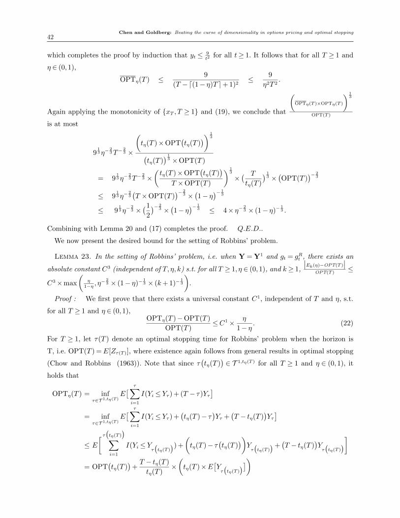
Chen and Goldberg: Beating the curse of dimensionality in options pricing and optimal stopping42
which completes the proof by induction that yt ≤ 9t2
for all t≥ 1. It follows that for all T ≥ 1 and
η ∈ (0,1),
OPTη(T ) ≤ 9
(T −d(1− η)T e+ 1)2≤ 9
η2T 2.
Again applying the monotonicity of {xT , T ≥ 1} and (19), we conclude that
(OPTη(T )×OPTη(T )
) 13
OPT(T )
is at most
913 η−
23T−
23 ×
(tη(T )×OPT
(tη(T )
)) 13
(tη(T )
) 13 ×OPT(T )
= 913 η−
23T−
23 ×
(tη(T )×OPT
(tη(T )
)T ×OPT(T )
) 13
×( T
tη(T )
) 13 ×
(OPT(T )
)− 23
≤ 913 η−
23(T ×OPT(T )
)− 23 ×
(1− η
)− 13
≤ 913 η−
23 ×
(1
2
)− 23 ×
(1− η
)− 13 ≤ 4× η− 2
3 × (1− η)−13 .
Combining with Lemma 20 and (17) completes the proof. Q.E.D..
We now present the desired bound for the setting of Robbins’ problem.
Lemma 23. In the setting of Robbins’ problem, i.e. when Y = Y1 and gt = gRt , there exists an
absolute constant C3 (independent of T,η, k) s.t. for all T ≥ 1, η ∈ (0,1), and k≥ 1,
∣∣Ek(η)−OPT(T )
∣∣OPT(T )
≤
C3×max
(η
1−η , η− 2
3 × (1− η)−13 × (k+ 1)−
13
).
Proof : We first prove that there exists a universal constant C1, independent of T and η, s.t.
for all T ≥ 1 and η ∈ (0,1),OPTη(T )−OPT(T )
OPT(T )≤C1× η
1− η. (22)
For T ≥ 1, let τ(T ) denote an optimal stopping time for Robbins’ problem when the horizon is
T, i.e. OPT(T ) =E[Zτ(T )], where existence again follows from general results in optimal stopping
(Chow and Robbins (1963)). Note that since τ(tη(T )
)∈ T 1,tη(T ) for all T ≥ 1 and η ∈ (0,1), it
holds that
OPTη(T ) = infτ∈T 1,tη(T )
E[ τ∑i=1
I(Yi ≤ Yτ ) + (T − τ)Yτ]
= infτ∈T 1,tη(T )
E[ τ∑i=1
I(Yi ≤ Yτ ) +(tη(T )− τ
)Yτ +
(T − tη(T )
)Yτ]
≤ E
[ τ(tη(T )
)∑i=1
I(Yi ≤ Yτ
(tη(T )
)) +
(tη(T )− τ
(tη(T )
))Yτ
(tη(T )
)+(T − tη(T )
)Yτ
(tη(T )
)]= OPT
(tη(T )
)+T − tη(T )
tη(T )×(tη(T )×E
[Yτ
(tη(T )
)])
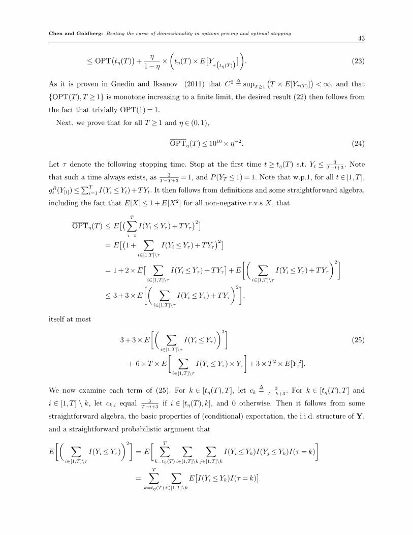
Chen and Goldberg: Beating the curse of dimensionality in options pricing and optimal stopping43
≤ OPT(tη(T )
)+
η
1− η×(tη(T )×E
[Yτ
(tη(T )
)]). (23)
As it is proven in Gnedin and Iksanov (2011) that C2 ∆= supT≥1
(T × E[Yτ(T )]
)<∞, and that
{OPT(T ), T ≥ 1} is monotone increasing to a finite limit, the desired result (22) then follows from
the fact that trivially OPT(1) = 1.
Next, we prove that for all T ≥ 1 and η ∈ (0,1),
OPTη(T )≤ 1010× η−2. (24)
Let τ denote the following stopping time. Stop at the first time t ≥ tη(T ) s.t. Yt ≤ 3T−t+3
. Note
that such a time always exists, as 3T−T+3
= 1, and P (YT ≤ 1) = 1. Note that w.p.1, for all t∈ [1, T ],
gRt (Y[t])≤∑T
i=1 I(Yi ≤ Yt)+TYt. It then follows from definitions and some straightforward algebra,
including the fact that E[X]≤ 1 +E[X2] for all non-negative r.v.s X, that
OPTη(T ) ≤ E[( T∑
i=1
I(Yi ≤ Yτ ) +TYτ)2]
= E[(
1 +∑
i∈[1,T ]\τ
I(Yi ≤ Yτ ) +TYτ)2]
= 1 + 2×E[ ∑i∈[1,T ]\τ
I(Yi ≤ Yτ ) +TYτ]
+E
[( ∑i∈[1,T ]\τ
I(Yi ≤ Yτ ) +TYτ
)2]
≤ 3 + 3×E[( ∑
i∈[1,T ]\τ
I(Yi ≤ Yτ ) +TYτ
)2],
itself at most
3 + 3×E[( ∑
i∈[1,T ]\τ
I(Yi ≤ Yτ ))2]
(25)
+ 6×T ×E[ ∑i∈[1,T ]\τ
I(Yi ≤ Yτ )×Yτ]
+ 3×T 2×E[Y 2τ ].
We now examine each term of (25). For k ∈ [tη(T ), T ], let ck∆= 3
T−k+3. For k ∈ [tη(T ), T ] and
i ∈ [1, T ] \ k, let ck,i equal 3T−i+3
if i ∈ [tη(T ), k], and 0 otherwise. Then it follows from some
straightforward algebra, the basic properties of (conditional) expectation, the i.i.d. structure of Y,
and a straightforward probabilistic argument that
E
[( ∑i∈[1,T ]\τ
I(Yi ≤ Yτ ))2]
= E
[ T∑k=tη(T )
∑i∈[1,T ]\k
∑j∈[1,T ]\k
I(Yi ≤ Yk)I(Yj ≤ Yk)I(τ = k)
]
=T∑
k=tη(T )
∑i∈[1,T ]\k
E[I(Yi ≤ Yk)I(τ = k)
]

Chen and Goldberg: Beating the curse of dimensionality in options pricing and optimal stopping44
+ 2T∑
k=tη(T )
∑i∈[1,T ]\k
∑j∈[i+1,T ]\k
E[I(Yi ≤ Yk)I(Yj ≤ Yk)I(τ = k)
]≤
T∑k=tη(T )
∑i∈[1,T ]\k
P (τ = k)×P(Yi ≤ ck|τ = k
)+ 2
T∑k=tη(T )
∑i∈[1,T ]\k
∑j∈[i+1,T ]\k
P (τ = k)×P(Yi ≤ ck, Yj ≤ ck|τ = k
)=
T∑k=tη(T )
∑i∈[1,T ]\k
P (τ = k)×P(Yi ≤ ck|Yi > ck,i
)+ 2
T∑k=tη(T )
∑i∈[1,T ]\k
∑j∈[i+1,T ]\k
P (τ = k)×P(Yi ≤ ck, Yj ≤ ck|Yi > ck,i, Yj > ck,j
)≤
T∑k=tη(T )
∑i∈[1,T ]\k
P (τ = k)×P (Yi ≤ ck)
+ 2T∑
k=tη(T )
∑i∈[1,T ]\k
∑j∈[i+1,T ]\k
P (τ = k)×P(Yi ≤ ck, Yj ≤ ck
)≤ T ×
T∑k=tη(T )
P (τ = k)× ck + 2×T 2×T∑
k=tη(T )
P (τ = k)× c2k; (26)
E
[ ∑i∈[1,T ]\τ
I(Yi ≤ Yτ )×Yτ]
=T∑
k=tη(T )
∑i∈[1,T ]\k
E[I(Yi ≤ Yk)×Yk× I(τ = k)
]≤
T∑k=tη(T )
∑i∈[1,T ]\k
P (τ = k)× ck×P (Yi ≤ ck|Yi > ck,i)
≤ T ×T∑
k=tη(T )
P (τ = k)× c2k. (27)
As similar arguments yield the inequality E[Y 2τ ] ≤
∑T
k=tη(T )P (τ = k)× c2k, we may combine (25)
with (26) - (27) and the fact that E[cτ ]≤(E[c2
τ ]) 1
2 to conclude that
OPTη(T )≤ 3 + 3×T ×( T∑k=tη(T )
P (τ = k)× c2k
) 12
+ 15×T 2×T∑
k=tη(T )
P (τ = k)× c2k. (28)
Now, we bound∑T
k=tη(T )P (τ = k)× c2k, with all arguments following from some straightforward
algebra, the i.i.d. structure of Y, several Taylor-series approximations, and the fact that for all
n≥ 1, the nth harmonic number∑n
i=11i
satisfies |∑n
i=11i− log(n)| ≤ 2. Then
∑T
k=tη(T )P (τ = k)×c2k
equals
T∑k=tη(T )
( k−1∏i=tη(T )
(1− 3
T − i+ 3
))×( 3
T − k+ 3
)3
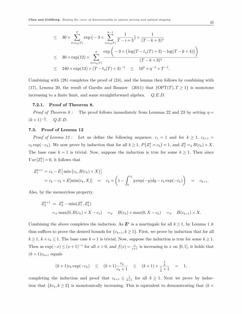
Chen and Goldberg: Beating the curse of dimensionality in options pricing and optimal stopping45
≤ 30×T∑
k=tη(T )
exp(− 3×
k−1∑i=tη(T )
1
T − i+ 3
)× 1
(T − k+ 3)3
≤ 30× exp(12)×T∑
k=tη(T )
exp
(− 3×
(log(T − tη(T ) + 3)− log(T − k+ 4)
))(T − k+ 3)3
≤ 240× exp(12)× (T − tη(T ) + 3)−2 ≤ 108× η−2×T−2.
Combining with (28) completes the proof of (24), and the lemma then follows by combining with
(17), Lemma 20, the result of Gnedin and Iksanov (2011) that {OPT(T ), T ≥ 1} is monotone
increasing to a finite limit, and some straightforward algebra. Q.E.D.
7.2.1. Proof of Theorem 8.
Proof of Theorem 8 : The proof follows immediately from Lemmas 22 and 23 by setting η =
(k+ 1)−15 . Q.E.D.
7.3. Proof of Lemma 12
Proof of Lemma 12 : Let us define the following sequence. c1 = 1 and for k ≥ 1, ck+1 =
ck exp(−ck). We now prove by induction that for all k≥ 1, P(Zk1 = ck
)= 1, and Zk2 =d B(ck)×X.
The base case k = 1 is trivial. Now, suppose the induction is true for some k ≥ 1. Then since
V ar[Zk1 ] = 0, it follows that
Zk+11 = ck−E
[min
(ck,B(ck)×X
)]= ck− ck×E[min(ck,X)] = ck×
(1−
∫ ck
0
y exp(−y)dy− ck exp(−ck))
= ck+1.
Also, by the memoryless property,
Zk+12 = Zk2 −min(Zk1 ,Z
k2 )
=d max(0,B(ck)×X − ck) =d B(ck)×max(0,X − ck) =d B(ck+1)×X.
Combining the above completes the induction. As Zk is a martingale for all k≥ 1, by Lemma 1 it
thus suffices to prove the desired bounds for {ck+1, k≥ 1}. First, we prove by induction that for all
k≥ 1, k× ck ≤ 1. The base case k= 1 is trivial. Now, suppose the induction is true for some k≥ 1.
Then as exp(−x)≤ (x+ 1)−1 for all x> 0, and f(x) = xx+1
is increasing in x on [0,1], it holds that
(k+ 1)ck+1 equals
(k+ 1)ck exp(−ck) ≤ (k+ 1)ck
ck + 1≤ (k+ 1)×
1k
1k
+ 1= 1,
completing the induction and proof that ck+1 ≤ 1k+1
for all k ≥ 1. Next we prove by induc-
tion that {kck, k ≥ 2} is monotonically increasing. This is equivalent to demonstrating that (k+
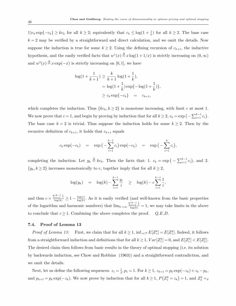
Chen and Goldberg: Beating the curse of dimensionality in options pricing and optimal stopping46
1)ck exp{−ck} ≥ kck for all k ≥ 2; equivalently that ck ≤ log(1 + 1k) for all k ≥ 2. The base case
k = 2 may be verified by a straightforward and direct calculation, and we omit the details. Now
suppose the induction is true for some k ≥ 2. Using the defining recursion of ck+1, the inductive
hypothesis, and the easily verified facts that w1(x)∆= x log(1 + 1/x) is strictly increasing on (0,∞)
and w2(x)∆= x exp(−x) is strictly increasing on [0,1], we have
log(1 +1
k+ 1) ≥ k
k+ 1log(1 +
1
k),
= log(1 +1
k) exp{− log(1 +
1
k)},
≥ ck exp{−ck} = ck+1,
which completes the induction. Thus {kck, k ≥ 2} is monotone increasing, with limit c at most 1.
We now prove that c= 1, and begin by proving by induction that for all k≥ 2, ck = exp(−∑k−1
i=1 ci).
The base case k = 2 is trivial. Thus suppose the induction holds for some k ≥ 2. Then by the
recursive definition of ck+1, it holds that ck+1 equals
ck exp(−ck) = exp(−
k−1∑i=1
ci)
exp(−ck) = exp(−
k∑i=1
ci),
completing the induction. Let yk∆= kck. Then the facts that: 1. ck = exp
(−∑k−1
i=1 ci), and 2.
{yk, k≥ 2} increases monotonically to c, together imply that for all k≥ 2,
log(yk) = log(k)−k−1∑i=1
yii≥ log(k)− c
k−1∑i=1
1
i,
and thus c×∑k−1i=1
1i
log(k)≥ 1− log(c)
log(k). As it is easily verified (and well-known from the basic properties
of the logarithm and harmonic numbers) that limk→∞
∑k−1i=1
1i
log(k)= 1, we may take limits in the above
to conclude that c≥ 1. Combining the above completes the proof. Q.E.D.
7.4. Proof of Lemma 13
Proof of Lemma 13: First, we claim that for all k≥ 1, infτ∈T E[Zkτ ] =E[Zk1 ]. Indeed, it follows
from a straightforward induction and definitions that for all k≥ 1, V ar[Zk1 ] = 0, and E[Zk1 ]<E[Zk2 ].
The desired claim then follows from basic results in the theory of optimal stopping (i.e. its solution
by backwards induction, see Chow and Robbins (1963)) and a straightforward contradiction, and
we omit the details.
Next, let us define the following sequences. z1 = 12, p1 = 1. For k≥ 1, zk+1 = pk exp(−zk)+zk−pk,
and pk+1 = pk exp(−zk). We now prove by induction that for all k≥ 1, P(Zk1 = zk
)= 1, and Zk2 =d

Chen and Goldberg: Beating the curse of dimensionality in options pricing and optimal stopping47
B(pk)×X. The base case k= 1 is trivial. Now, suppose the induction is true for some k≥ 1. Then
since V ar[Zk1 ] = 0, it follows that
Zk+11 = zk−E
[min
(zk,B(pk)×X
)]= zk− pk×E[min(zk,X)] = zk− pk×
(∫ zk
0
y exp(−y)dy+ zk exp(−zk))
= zk+1.
Also, by the memoryless property,
Zk+12 = Zk2 −min(Zk1 ,Z
k2 )
=d max(0,B(pk)×X − zk) =d B(pk)×max(0,X − zk) =d B(pk+1)×X.
Combining the above completes the induction.
It follows that for all k≥ 1, pk+1− pk = zk+1− zk, and thus pk = zk + (p1− z1) = zk + 12. Plugging
back into the original definitions of pk and zk, we find that zk+1 = (zk + 12) exp(−zk) − 1
2. The
fact that infτ∈T E[Zkτ ] =E[Zk1 ], combined with Lemma 1 and Theorem 2, implies that {zk, k ≥ 1}
converges monotonically to 0. It then follows from a straightforward application of L’Hopital’s rule
that
limk→∞
zk+1
zk= lim
k→∞
(zk + 12) exp(−zk)− 1
2
zk= lim
z↓0
(z+ 12) exp(−z)− 1
2
z=
1
2,
from which the desired result follows. Q.E.D.
7.5. Proof of Lemma 14
Proof of Lemma 14: Let us define the following sequences. Let a1 = 2, and b1 = 1. For k ≥ 1,
let ak+1 = ak− 12akbk, and bk+1 = bk(1− bk
2). We now prove by induction that for all k≥ 1, P
(Zk1 =
akbk2
)= 1, and Zk2 =d B(bk)×U(ak). The base case k = 1 is trivial. Now, suppose the induction is
true for some k ≥ 1. Then since V ar[Zk1 ] = 0, and a straightforward induction demonstrates that
bk ∈ (0,1) and ak > 0, it follows from a straightforward probabilistic argument that
Zk+12 =d max
(0,B(bk)×U(ak)−
akbk2
)=d B
(bk(1−
bk2
))U(ak−
akbk2
),
completing the proof that Zk+12 =d B(bk+1)×U(ak+1). The desired induction then follows from the
martingale property.
Note that the definition of the recursions for ak+1 and bk+1 implies thatak+1
ak=
bk+1
bk= 1− bk
2
for all k ≥ 1. It follows that for all k ≥ 1, akbk
= a1b1
= 2, and hence ak = 2bk. It follows from Lemma
21 that {k × bk, k ≥ 2} is monotone increasing, with limit 2. As Zk1 = ak×bk2
= b2k, it follows that
{k2Zk1 , k≥ 2} is monotone increasing with limit 4. Combining the above with the fact that Zk is a
martingale and Lemma 1 completes the proof. Q.E.D.

Chen and Goldberg: Beating the curse of dimensionality in options pricing and optimal stopping48
7.6. Proof of Lemma 16
Proof of Lemma 16 : Recall that
fk(ε, δ) = 102(k−1)2ε−2(k−1)(T + 2)k−1(1 + log(
1
δ) + log(
1
ε) + log(T )
)k−1,
and N(ε, δ) = d 12ε2
log( 2δ)e. As it is easily verified that 1 < log(8)
2, and thus for all ε, δ ∈ (0,1),
N( ε4, δ
4) ≤ 8.5
ε2log( 8
δ) and N( ε
4, δ
4) + 1 ≤ 9
ε2log( 8
δ), we argue as follows.
(N( ε
4, δ
4) + 1
)×(T + 2
)×
fk(ε4, δ
4N( ε4 ,δ4 )T
)is at most
9
ε2× log(
8
δ)× (T + 2)× fk
( ε4,
δ34ε2
log( 8δ)T
)≤ 9
ε2× log(
8
δ)× (T + 2)
× 102(k−1)2(T + 2)k−1(ε
4)−2(k−1)
(1 + log
(34
ε2log(
8
δ)T
δ
)+ log
(4
ε) + log(T )
)k−1
≤ 9× log(8
δ)× (T + 2)k× ε−2k× 102(k−1)2 × 16k−1
×
(1 + log(34) + 2 log(
1
ε) + log(
8
δ) + log(
T
δ) + log(4) + log(
1
ε) + log(T )
)k−1
≤ 9× log(8
δ)× (T + 2)k× ε−2k× 102(k−1)2 × 16k−1×
(10 + 3 log(
1
ε) + 2 log(
1
δ) + 2 log(T )
)k−1
≤ 9× (T + 2)k× ε−2k× 102(k−1)2 × 16k−1×
(10 + 3 log(
1
ε) + 2 log(
1
δ) + 2 log(T )
)k
≤ 10k+1× (T + 2)k× ε−2k× 102(k−1)2 × 10²(k−1)×
(1 + log(
1
ε) + log(
1
δ) + log(T )
)k,
which is further bounded by fk+1
(ε, δ)
since 2k2−(k+1+2(k−1)2 +2(k−1)
)= k−1≥ 0. Q.E.D.
7.7. Proof of Corollary 2:
Proof of Corollary 2: In light of Theorems 6 and 2, by a union bound and the triangle inequality
it suffices to individually approximate each of the first d 2εe of the Hi, each to within additive error
ε2
(d 2εe)−1
with probability 1− δ(d 2εe)−1
. After accounting for the cost of averaging the d 2εe values,
and combining with the monotonicities of fk and some straightforward algebra, we find that the
the computational cost divided by C +G+ 1 is at most
d 2ε e∑i=1
fi+1
(ε
2
(d2εe)−1
, δ(d2εe)−1)
+ d2εe+ 1
≤ d2εefd 2ε e+1
(ε26,δε
3
)+ d2
εe+ 1
≤ 6ε−1fd 2ε e+1
(ε26,δε
3
)

Chen and Goldberg: Beating the curse of dimensionality in options pricing and optimal stopping49
≤ 6ε−1102(3ε−1)2(ε2
6)−2(3ε−1)(T + 2)3ε−1(
1 + log(3
εδ) + log(
6
ε2) + log(T )
)3ε−1
= 1018ε−2
66ε−1+1ε−12ε−1−1(T + 2)3ε−1(1 + log(3) + log(6) + 3 log(
1
ε) + log(
1
δ) + log(T )
)3ε−1
≤ 1018ε−2
exp
(log(6)(7ε−1) + log(
1
ε)(13ε−1)
)(T + 2)3ε−1
×(1 + log(3) + log(6) + 3 log(
1
ε) + log(
1
δ) + log(T )
)3ε−1
≤ 1018ε−2
exp(14ε−2 + 13ε−2
)(T + 2)3ε−1(
1 + log(3) + log(6) + 3 log(1
ε) + log(
1
δ) + log(T )
)3ε−1
= exp
((27 + 18 log(10)
)ε−2
)(T + 2)3ε−1(
1 + log(3) + log(6) + 3 log(1
ε) + log(
1
δ) + log(T )
)3ε−1
≤ exp(80ε−2)27ε−1
T 3ε−1(5 + 3 log(
1
ε) + log(
1
δ) + log(T )
)3ε−1
≤ exp(80ε−2)(5000)ε−1
T 3ε−1(1 + log(
1
ε) + log(
1
δ) + log(T )
)3ε−1
≤ exp(100ε−2)T 3ε−1(1 + log(
1
ε) + log(
1
δ) + log(T )
)3ε−1
≤ exp(100ε−2)T 6ε−1
× 23ε−1
×(1 + log(
1
ε) + log(
1
δ))3ε−1
since 1 + log(1
ε) + log(
1
δ) + log(T )≤ 2T
(1 + log(
1
ε) + log(
1
δ))
≤ exp(100ε−2)T 6ε−1
× 23ε−1
(e
ε)3ε−1(
1 + log(1
δ))3ε−1
since 1 + log(1
ε) + log(
1
δ)≤ e
ε
(1 + log(
1
δ))
≤ exp(100ε−2)×T 6ε−1
× e6ε−1
× exp(3ε−1 log(
1
ε))×(1 + log(
1
δ))3ε−1
≤ exp(200ε−2)×T 6ε−1
×(1 + log(
1
δ))6ε−1
.
The analysis for the number of calls to the base simulator follows nearly identically, and we omit
the details. Combining the above completes the proof. Q.E.D.
7.8. Proof of Theorem 9
We begin by proving some auxiliary lemmas. First, we bound the error introduced by our trunca-
tion.
Lemma 24. For all U > 0,
0≤ OPT−U × supτ∈T
E[Z1U,τ ]≤ (M2)
12 ×
(M1
U
) 12 .
Proof : Non-negativity follows from the fact that w.p.1 Z1t ≥ U × Z1
U,t for all t ∈ [1, T ]. To
prove the other direction, let τ∗ denote an optimal stopping time for the problem supτ∈T E[Z1τ ],
where existence follows from Chow and Robbins (1963). Then by a straightforward coupling and
rescaling,
E[Z1τ∗ ]−U ×E[Z1
U,τ∗ ] ≤ E[Z1τ∗I(Z1τ∗ >U
)]

Chen and Goldberg: Beating the curse of dimensionality in options pricing and optimal stopping50
≤ E[Z1τ∗I(
maxt∈[1,T ]
Z1t >U
)]≤ E
[(maxt∈[1,T ]
Z1t
)× I(
maxt∈[1,T ]
Z1t >U
)]≤ (M2)
12 ×
(P(
maxt∈[1,T ]
Z1t >U
)) 12
by Cauchy-Schwarz
≤ (M2)12 ×
(M1
U
) 12 by Markov’s inequality,
completing the proof. Q.E.D.
Next, we prove that if γ0 is not too large, then OPTM1
cannot be too small.
Lemma 25. OPT≥ 427× γ−1
0 ×M1.
Proof : Recall the celebrated Paley-Zygmund inequality, i.e. the fact that for any δ ∈ (0,1) and
non-negative r.v. X,
P(X > δE[X]
)≥ (1− δ)2× (E[X])2
E[X2]. (29)
Now, for δ ∈ (0,1), consider the stopping time τδ which stops the first time that that Z1t ≥ δ×M1,
and stops at time T if no such time exists in [1, T ]. Then by non-negativity and (29),
E[Z1τδ
] ≥ δ× (1− δ)2× (M1)3
M2
.
Optimizing over δ (a straightforward exercise in calculus) then completes the proof. Q.E.D.
By combining Lemmas 24 - 25, we are led to the following corollary.
Corollary 5. For all U > 0,
0≤ OPT−U × supτ∈T
E[Z1U,τ ]≤
27
4× (γ0)
32 ×
(M1
U
) 12 × OPT.
Proof : It follows from Lemma 25 that
(M2)12
OPT≤ 27
4× (M2)
32
(M1)3
=27
4× (γ0)
32 .
Combining with Lemma 24 completes the proof. Q.E.D.
We now complete the proof of Theorem 9.
Proof of Theorem 9 : Note that for all U > 0,
supτ∈T
E[Z1U,τ ] = 1− inf
τ∈TE[Z1,−
U,τ ]; (30)
and Theorem 2 implies that for all U > 0 and k≥ 1,
1−E−U,k−1
k+ 1≤ sup
τ∈TE[Z1
U,τ ]≤ 1−E−U,k. (31)

Chen and Goldberg: Beating the curse of dimensionality in options pricing and optimal stopping51
It then follows from Corollary 5 and the triangle inequality that∣∣∣∣OPT−U ×(1−E−U,k + z
)∣∣∣∣≤ 27
4× (γ0)
32 ×
(M1
U
) 12 × OPT +U ×
(|z|+ (k+ 1)−1
).
Furthermore,
U
OPT=
U
M1
× M1
OPT
≤ U
M1
× M1
427× (M1)3
M2
=27
4× γ0×
U
M1
.
Combining the above with the triangle inequality, the fact that γ0 ≥ 1 by Jensen’s inequality, and
some straightforward algebra completes the proof. Q.E.D.
7.9. Proof of Theorem 7
Proof of Theorem 7 : Recall that U0 = 104× γ30 × ε−2×M1. Let k0
∆= d( U0
M1)32 e. It then follows
from the definition of A, Theorem 10, and a straightforward union bound and application of
the triangle inequality that with probability at least 1− δ, A returns a random number X s.t.
|X −E−U0,k0| ≤ ( U0
M1)−
32 . Thus by Theorem 9, to prove the first part of the theorem (i.e. that the
algorithm returns a value with the stated guarantees) it suffices to prove that 7×γ320 ×
(U0M1×(2×
( U0M1
)−32
)+ ( U0
M1)−
12
)≤ ε, equivalently that 21γ
320 ( U0
M1)−
12 ≤ ε. Since
21γ320 (U0
M1
)−12 = 21× γ
320 ×
(104× γ3
0 × ε−2
)− 12
≤ ε,
combining the above completes the proof.
Next, let us prove the second part of the theorem regarding the runtime analysis. Recall that
fk(ε′, δ′) = 102(k−1)2 × ε′−2(k−1)× (T + 2)k−1×
(1 + log(
1
δ′) + log(
1
ε′) + log(T )
)k−1.
Carefully accounting for all operations performed by A, and applying Theorem 10 and the mono-
tonicities of various functions, we find that the computational cost divided by C + G + 1 is at
most
16 + d( U0
M1
)32 e× 4× f
d( U0M1
)32 e+1
(((U0
M1
)32 + 1
)−2, δ×
((U0
M1
)32 + 1
)−1)
+ d( U0
M1
)32 e
≤ 102(U0
M1
)32 fd( U0M1
)32 e+1
(1
4(U0
M1
)−3,1
4δ(U0
M1
)−32)
≤ 102× (U0
M1
)32 × 10
8(U0M1
)3 ×(4(U0
M1
)3)4(
U0M1
)32
× (T + 2)2(U0M1
)32
×(
1 + log(4) + log(1
δ) +
3
2log(
U0
M1
) + log(4) + 3 log(U0
M1
) + log(T )
)2(U0M1
)32

Chen and Goldberg: Beating the curse of dimensionality in options pricing and optimal stopping52
≤ 1025(
U0M1
)3 ×T 2(U0M1
)32 ×
(10 + log(
1
δ) + 5 log(
U0
M1
) + log(T )
)2(U0M1
)32
since 102 ≤ 102(U0M1
)3
, (U0
M1
)32 ≤ 10
(U0M1
)3
, 44(U0M1
)32 ≤ 10
3(U0M1
)3
,
(U0
M1
)12(
U0M1
)32 ≤ exp
(12(
U0
M1
)52)≤ 10
7(U0M1
)3
, (T + 2)2(U0M1
)32 ≤ 10
(U0M1
)3 ×T 2(U0M1
)32
≤ 1027(
U0M1
)3 ×T 2(U0M1
)32 ×
(1 + log(
1
δ) + log(
U0
M1
) + log(T )
)2(U0M1
)32
≤ 10
(1014γ90ε
−6)×T
(107γ
920 ε−3)×(
1 + log(1
δ) + 4 log(10) + 3 log(γ0) + 2 log(
1
ε) + log(T )
)(107γ920 ε−3)
≤ 10
(1015γ90ε
−6)×T
(107γ
920 ε−3)×(
1 + log(1
δ) + log(γ0) + log(
1
ε) + log(T )
)(107γ920 ε−3)
≤ exp(1016γ9
0ε−6)×T
(107γ
920 ε−3)×(
1 + log(1
δ) + log(γ0) + log(
1
ε) + log(T )
)(107γ920 ε−3)
≤ exp(1017γ9
0ε−6)×T 108γ
920 ε−3
×(
1 + log(1
δ) + log(γ0) + log(
1
ε)
)107γ920 ε−3
≤ exp(1018γ9
0ε−6)×T 108γ
920 ε−3
×(
1 + log(1
δ) + log(γ0)
)107γ920 ε−3
≤ exp(1018γ9
0ε−6)×T 108γ
920 ε−3
× (2γ0)107γ920 ε−3
×(1 + log(
1
δ))107γ
920 ε−3
≤ exp(1020γ9
0ε−6)×T 108γ
920 ε−3
×(1 + log(
1
δ))108γ
920 ε−3
.
The analysis for the number of calls to the base simulator follows nearly identically, and we omit
the details. Combining the above completes the proof. Q.E.D.
Acknowledgements
The authors gratefully acknowledge Sid Banerjee, Erhan Bayraktar, Denis Belomestny, Thomas
Bruss, Agostino Capponi, Jim Dai, Mark Davis, Vivek Farias, Paul Glasserman, Nir Halman,
Shane Henderson, Saul Jacka, Bobby Kleinberg, Ozalp Ozer, Philip Protter, Chris Rogers, John
Schoenmakers, Timur Tankayev, John Tsitsiklis, Alberto Vera, and David Williamson for several
helpful conversations and insights. The authors especially thank Jim Dai for his organization of a
seminar series on Reinforcement Learning for Processing Networks, as well as all participants of
that seminar series. The authors also thank the organizers and participants of the 2018 Symposium
on optimal stopping in honor of Larry Shepp held at Rice University.
Chen and Goldberg: Beating the curse of dimensionality in options pricing and optimal stopping53
References
Abolhassani, M., Ehsani, S., Esfandiari, H., HajiAghayi, M., Kleinberg, R., and Lucier, B. (2017, June).
“Beating 1-1/e for ordered prophets.” In Proceedings of the 49th Annual ACM SIGACT Symposium
on Theory of Computing (pp. 61-71). ACM.
Achdou, Y., and O. Pironneau. Computational methods for option pricing. Vol. 30. Siam, 2005.
Agarwal, A., and S. Juneja. “Comparing optimal convergence rate of stochastic mesh and least squares
method for bermudan option pricing.” Proceedings of the 2013 Winter Simulation Conference: Simu-
lation: Making Decisions in a Complex World. IEEE Press, 2013.
Agarwal, A., S. Juneja, and R. Sircar. “American options under stochastic volatility: control variates, matu-
rity randomization and multiscale asymptotics.” Quantitative Finance 16.1 (2016): 17-30.
Ahn, S., H. Bae, H. Koo, and K. Lee. “A survey on American options: old approaches and new trends.”
Bulletin of the Korean Mathematical Society 48, no. 4 (2011): 791-812.
Ahuja, R., T. Magnanti, and J.B. Orlin. Network flows. Pearson Education, 2014.
Andersen, L., and M. Broadie. “Primal-dual simulation algorithm for pricing multidimensional American
options.” Management Science 50.9 (2004): 1222-1234.
Arlotto, A., and I. Gurvich. “Uniformly bounded regret in the multi-secretary problem.” arXiv preprint
arXiv:1710.07719 (2017).
Arora, S., B. Barak, M. Brunnermeier, and R. Ge. “Computational complexity and information asymmetry
in financial products.” Communications of the ACM 54, no. 5 (2011): 101-107.
Avramidis, A., and H. Matzinger. “Problems in financial engineering: convergence of the stochastic mesh
estimator for pricing American options.” Proceedings of the 34th conference on Winter simulation:
exploring new frontiers. Winter Simulation Conference, 2002.
Aydogan, Burcu, Umit Aksoy, and Omur Ugur. “On the methods of pricing American options: case study.”
Annals of Operations Research 260.1-2 (2018): 79-94.
Bandi, C., and D. Bertsimas. ”Robust option pricing.” European Journal of Operational Research 239, no.
3 (2014): 842-853.
Bank, P., and H. Follmer. “American Options, Multiarmed Bandits, and Optimal Consumption Plans: A
Unifying View.” Paris-Princeton Lectures on Mathematical Finance (2003).
Bayer, C., P. Friz, and J. Gatheral. ”Pricing under rough volatility.” Quantitative Finance 16.6 (2016):
887-904.
Bayraktar, E., and S. Yao. “On the robust optimal stopping problem.” SIAM Journal on Control and
Optimization 52.5 (2014): 3135-3175.
Becker, S., P. Cheridito, and A. Jentzen. “Deep optimal stopping.” arXiv preprint arXiv:1804.05394 (2018).
Chen and Goldberg: Beating the curse of dimensionality in options pricing and optimal stopping54
Belomestny, D., J. Schoenmakers, and F. Dickmann. “Multilevel dual approach for pricing American style
derivatives.” Finance and Stochastics 17.4 (2013): 717-742.
Belomestny, D., M. Ladkau, and J. Schoenmakers. “Multilevel Simulation Based Policy Iteration for Optimal
Stopping–Convergence and Complexity.” SIAM/ASA Journal on Uncertainty Quantification 3.1 (2015):
460-483.
Belomestny, D. “Solving optimal stopping problems via empirical dual optimization.” The Annals of Applied
Probability 23.5 (2013): 1988-2019.
Belomestny, D., R. Hildebrand, and J. Schoenmakers. “Optimal stopping via pathwise dual empirical max-
imisation.” Applied Mathematics and Optimization (2017): 1-27.
Belomestny, D., S. Hafner, and M. Urusov. “Regression-based complexity reduction of the nested Monte
Carlo methods.” (2018).
Belomestny, D., and G. Milstein. “Monte Carlo evaluation of American options using consumption processes.”
International Journal of theoretical and applied finance 9.04 (2006): 455-481.
Belomestny, D., C. Bender, and J. Schoenmakers. “True upper bounds for Bermudan products via nonnested
Monte Carlo.” Mathematical Finance: An International Journal of Mathematics, Statistics and Finan-
cial Economics 19.1 (2009): 53-71.
Belomestny, D. “Pricing Bermudan options by nonparametric regression: optimal rates of convergence for
lower estimates.” Finance and Stochastics 15.4 (2011): 655-683.
Belomestny, D. “On the rates of convergence of simulation-based optimization algorithms for optimal stop-
ping problems.” The Annals of Applied Probability 21.1 (2011): 215-239.
Belomestny, D., and J. Schoenmakers. Advanced Simulation-Based Methods for Optimal Stopping and Con-
trol: With Applications in Finance. Springer, 2018.
Bender, C., and J. Schoenmakers. “An iterative method for multiple stopping: convergence and stability.”
Advances in applied probability 38.3 (2006): 729-749.
Bender, C., A. Kolodko, and J. Schoenmakers. “Policy iteration for american options: overview.” Monte
Carlo Methods and Applications 12.5 (2006): 347.
Bender, C., A. Kolodko, and J. Schoenmakers. “Enhanced policy iteration for American options via scenario
selection.” Quantitative Finance 8.2 (2008): 135-146.
Bender, C., J. Schoenmakers, and J. Zhang. “Dual representations for general multiple stopping problems.”
Mathematical Finance 25.2 (2015): 339-370.
Bender, C., C. Gartner, and N. Schweizer. “Pathwise dynamic programming.” Mathematics of Operations
Research (2018).
Bertsimas, D., and I. Popescu. “On the relation between option and stock prices: a convex optimization
approach.” Operations Research, 50(2):358 374, 2002.
Chen and Goldberg: Beating the curse of dimensionality in options pricing and optimal stopping55
Beveridge, C., M. Joshi, and R. Tang. “Practical policy iteration: Generic methods for obtaining rapid and
tight bounds for Bermudan exotic derivatives using Monte Carlo simulation.” Journal of Economic
Dynamics and Control 37.7 (2013): 1342-1361.
Bezerra, S., A. Ohashi, and F. Russo. “Discrete-type approximations for non-Markovian optimal stopping
problems: Part II.” arXiv preprint arXiv:1707.05250 (2017).
Bhandari, J., D. Russo, and R. Singal. ”A Finite Time Analysis of Temporal Difference Learning With Linear
Function Approximation.” arXiv preprint arXiv:1806.02450 (2018). Accepted to COLT 2018.
Blanchet, J., G. Gallego, and V. Goyal. ”A markov chain approximation to choice modeling.” Operations
Research 64, no. 4 (2016): 886-905.
Blanchet, J., X. Chen, and J. Dong. “epsilon-Strong Simulation of Multidimensional Stochastic Differential
Equations via Rough Path Analysis.” Annals of Applied Probability, 27, (2017), 275-339.
Bolia, N., S. Juneja, and P. Glasserman. “Function-approximation-based importance sampling for pricing
American options.” Proceedings of the 36th conference on Winter simulation. Winter Simulation Con-
ference, 2004.
Bolia, N., and S. Juneja. “Function-approximation-based perfect control variates for pricing American
options.” Simulation Conference, 2005 Proceedings of the Winter. IEEE, 2005.
Booth, Heather, and Robert Endre Tarjan. ”Finding the minimum-cost maximum flow in a series-parallel
network.” Journal of Algorithms 15, no. 3 (1993): 416-446.
Bouchard, B., and X. Warin. “Monte-Carlo valuation of American options: facts and new algorithms to
improve existing methods.” Numerical methods in finance. Springer, Berlin, Heidelberg, 2012. 215-255.
Boyle, P., A. Kolkiewicz, and K. Tan. “An improved simulation method for pricing high-dimensional Amer-
ican derivatives.” Mathematics and Computers in Simulation 3.62 (2003): 315-322.
Braverman, M., and K. Pasricha. “The computational hardness of pricing compound options.” Proceedings
of the 5th conference on Innovations in theoretical computer science. ACM, 2014.
Broadie, M., and M. Cao. “Improved lower and upper bound algorithms for pricing American options by
simulation.” Quantitative Finance 8.8 (2008): 845-861.
Broadie, M., and P. Glasserman. “Pricing American-style securities using simulation.” Journal of economic
dynamics and control 21.8-9 (1997): 1323-1352.
Broadie, M., P. Glasserman, and Z. Ha. “Pricing American options by simulation using a stochastic mesh
with optimized weights.” Probabilistic Constrained Optimization. Springer, Boston, MA, 2000. 26-44.
Broadie, M., and P. Glasserman. “A stochastic mesh method for pricing high-dimensional American options.”
Journal of Computational Finance 7 (2004): 35-72.
Broadie, M., and J. Detemple. “Anniversary article: Option pricing: Valuation models and applications.”
Management science 50.9 (2004): 1145-1177.
Chen and Goldberg: Beating the curse of dimensionality in options pricing and optimal stopping56
Brown, D., J. Smith, and P. Sun. “Information relaxations and duality in stochastic dynamic programs.”
Operations research 58.4-part-1 (2010): 785-801.
Brown, D., and M. Haugh. “Information relaxation bounds for infinite horizon markov decision processes.”
Operations Research 65.5 (2017): 1355-1379.
Brucker, P. ”An O (nlogn)-algorithm for the minimum cost flow problem in trees.” In Selected Topics in
Operations Research and Mathematical Economics, pp. 299-306. Springer, Berlin, Heidelberg, 1984.
Bruss, F. “What is known about Robbins’ problem?.” Journal of applied probability 42.1 (2005): 108-120.
Buchbinder, N., K. Jain, and M. Singh. “Secretary problems via linear programming.” In International
Conference on Integer Programming and Combinatorial Optimization, pp. 163-176. Springer, Berlin,
Heidelberg, 2010.
Bumpensanti, P., and H. Wang. “A Re-solving Heuristic for Dynamic Resource Allocation with Uniformly
Bounded Revenue Loss.” arXiv preprint arXiv:1802.06192 (2018).
Carmona, R., and N. Touzi. “Optimal multiple stopping and valuation of swing options.” Mathematical
Finance 18.2 (2008): 239-268.
Chalasani, P., and S. Jha. “Randomized stopping times and American option pricing with transaction costs.”
Mathematical Finance 11, no. 1 (2001): 33-77.
Chandramouli, S., and M. Haugh. “A unified approach to multiple stopping and duality.” Operations
Research Letters 40.4 (2012): 258-264.
Chandramouli, S. “A Convex Optimization Approach to Multiple Stopping: Pricing Chooser Caps and Swing
Options.”
Chen, N., and P. Glasserman. “Additive and multiplicative duals for American option pricing.” Finance and
Stochastics 11.2 (2007): 153-179.
Chen, N., and J. Hong. “Monte Carlo simulation in financial engineering.” Simulation Conference, 2007
Winter. IEEE, 2007.
Chen, Y., and M. Wang. “Lower Bound On the Computational Complexity of Discounted Markov Decision
Problems.” arXiv preprint arXiv:1705.07312 (2017).
Chow, Y., and H. Robbins. “On optimal stopping rules.” Zeitschrift fur Wahrscheinlichkeitstheorie und
verwandte Gebiete 2.1 (1963): 33-49.
Christensen, S. “A Method for Pricing American Options Using SemiInfinite Linear Programming.” Math-
ematical Finance 24.1 (2014): 156-172.
Christiano, P., J. Kelner, A. Madry, D. Spielman, and S. Teng. “Electrical flows, laplacian systems, and
faster approximation of maximum flow in undirected graphs.” In Proceedings of the forty-third annual
ACM symposium on Theory of computing, pp. 273-282. ACM, 2011.
Chen and Goldberg: Beating the curse of dimensionality in options pricing and optimal stopping57
Clement, E., D. Lamberton, and P. Protter. “An analysis of a least squares regression method for American
option pricing.” Finance and Stochastics 6.4 (2002): 449-471.
Cohen, E. ”Approximate max-flow on small depth networks.” SIAM Journal on Computing 24, no. 3 (1995):
579-597.
Cont, R., and P. Tankov. Financial Modelling with jump processes. (2003).
Cooper, W., and B. Rangarajan. ”Performance guarantees for empirical markov decision processes with
applications to multiperiod inventory models.” Operations Research 60, no. 5 (2012): 1267-1281.
Correa, J., P. Foncea, R. Hoeksma, T. Oosterwijk, and T. Vredeveld. “Posted price mechanisms for a random
stream of customers.” In Proceedings of the 2017 ACM Conference on Economics and Computation,
pp. 169-186. ACM, 2017.
Daskalakis, C., G. Kamath, and J. Wright. ”Which distribution distances are sublinearly testable?.” In
Proceedings of the Twenty-Ninth Annual ACM-SIAM Symposium on Discrete Algorithms, pp. 2747-
2764. Society for Industrial and Applied Mathematics, 2018.
Davis, M., and I. Karatzas, “A deterministic approach to optimal stopping.” In Probability, Statistics and
Optimization: a Tribute to Peter Whittle, ed. F.P. Kelly, Wiley 1994.
Del Moral, P., P. Hu, N. Oudjane, and B. Remillard. “On the Robustness of the Snell envelope.” SIAM
Journal on Financial Mathematics 2, no. 1 (2011): 587-626.
Dendievel, R., and Y. Swan. “One step further: an explicit solution to Robbins’ problem when n= 4.”
Mathematica applicanda (2016).
Desai, V., V. Farias, and C. Moallemi. “Pathwise optimization for optimal stopping problems.” Management
Science 58.12 (2012): 2292-2308.
Dieker, A. “Simulation of fractional Brownian motion.” MSc theses, University of Twente, Amsterdam, The
Netherlands (2004).
Duffie, D. Dynamic asset pricing theory. Princeton University Press, 2010.
Egloff, D. “Monte Carlo algorithms for optimal stopping and statistical learning.” The Annals of Applied
Probability 15.2 (2005): 1396-1432.
Egloff, D., M. Kohler, and N. Todorovic. “A dynamic look-ahead Monte Carlo algorithm for pricing Bermudan
options.” The Annals of Applied Probability 17.4 (2007): 1138-1171.
Faden, A. “The existence of regular conditional probabilities: necessary and sufficient conditions.” The Annals
of Probability (1985): 288-298.
Ferguson, T. “Who solved the secretary problem?.” Statistical science (1989): 282-289.
Fujii, M., K. Matsumoto, and K. Tsubota. “Simple improvement method for upper bound of American
option.” Stochastics An International Journal of Probability and Stochastic Processes 83.4-6 (2011):
449-466.
Chen and Goldberg: Beating the curse of dimensionality in options pricing and optimal stopping58
Gilbert, J. P., and F. Mosteller. (1966). “Recognizing the Maximum of a Sequence.” Journal of the American
Statistical Association, 61(313), 35-73.
Glasserman, P. Monte Carlo methods in financial engineering. Vol. 53. Springer Science and Business Media,
2013.
Glasserman, P., and B. Yu. “Simulation for American options: Regression now or regression later?.” Monte
Carlo and Quasi-Monte Carlo Methods 2002. Springer, Berlin, Heidelberg, 2004. 213-226.
Glasserman, P., and B. Yu. “Number of paths versus number of basis functions in American option pricing.”
The Annals of Applied Probability 14.4 (2004): 2090-2119.
Gnedin, A., and A. Iksanov. “Moments of random sums and Robbins’ problem of optimal stopping.” Journal
of Applied Probability 48.4 (2011): 1197-1199.
Goldberg, A., and R. Tarjan. A parallel algorithm for finding a blocking flow in an acyclic network. No.
CS-TR-186-88. PRINCETON UNIV NJ DEPT OF COMPUTER SCIENCE, 1988.
Goldenshluger, A., and A. Zeevi. “Optimal Stopping of a Random Sequence with Unknown Distribution.”
(2017).
Halman, N., D. Klabjan, C. Li, J. Orlin, and D. Simchi-Levi. “Fully polynomial time approximation schemes
for stochastic dynamic programs.” SIAM Journal on Discrete Mathematics 28, no. 4 (2014): 1725-1796.
Halman, N., G. Nannicini, and J. Orlin. “A Computationally Efficient FPTAS for Convex Stochastic Dynamic
Programs”, SIAM J. Optimization 25, pp. 317-350, 2015.
Halman, N. Provably near-optimal approximation schemes for implicit stochastic and for sample-based
dynamic programs. Technical Report 4952, Optimization Online, 2015.
Halman, N., and G. Nannicini. ”Toward breaking the curse of dimensionality: an FPTAS for stochastic
dynamic programs with multidimensional action and scalar state.” (2017).
Haug, E. The complete guide to option pricing formulas. Vol. 2. New York: McGraw-Hill, 2007.
Haugh, M., and L. Kogan. “Pricing American options: a duality approach.” Operations Research 52.2 (2004):
258-270.
Haugh, M., and L. Kogan. “Duality theory and approximate dynamic programming for pricing American
options and portfolio optimization.” Handbooks in operations research and management science 15
(2007): 925-948.
Hepperger, P. “Pricing high-dimensional Bermudan options using variance-reduced Monte-Carlo methods.”
Journal of Computational Finance 16.3 (2013): 99-126.
Hill, T., and R. Kertz. “Stop rule inequalities for uniformly bounded sequences of random variables.” Trans-
actions of the American Mathematical Society 278.1 (1983): 197-207.
Hill, T., and R. Kertz. “A survey of prophet inequalities in optimal stopping theory.” Contemp. Math 125
(1992): 191-207.
Chen and Goldberg: Beating the curse of dimensionality in options pricing and optimal stopping59
Hoffman, A. ”On greedy algorithms that succeed.” Surveys in combinatorics 1985 (1985): 97-112.
Hoffman, Alan J. ”On greedy algorithms for series parallel graphs.” Mathematical programming 40, no. 1-3
(1988): 197-204.
Hoffman, A. ”On simple combinatorial optimization problems.” In Selected Papers Of Alan J Hoffman: With
Commentary, pp. 348-352. 2003.
Hong, J., and S. Juneja. “Estimating the mean of a non-linear function of conditional expectation.” Winter
Simulation Conference. Winter Simulation Conference, 2009.
Hutzenthaler, M., A. Jentzen, T. Kruse, T. Nguyen, and P. von Wurstemberger. ”Overcoming the curse of
dimensionality in the numerical approximation of semilinear parabolic partial differential equations.”
arXiv preprint arXiv:1807.01212 (2018).
Ibanez, A., and F. Zapatero. “Monte Carlo valuation of American options through computation of the optimal
exercise frontier.” Journal of Financial and Quantitative Analysis 39.2 (2004): 253-275.
Ibanez, A., and C. Velasco. “Recursive lower-and dual upper-bounds for Bermudan-style options.” (2017).
Available at SSRN: https://ssrn.com/abstract=2512659.
Jamshidian, F. “The duality of optimal exercise and domineering claims: A DoobMeyer decomposition
approach to the Snell envelope.” Stochastics An International Journal of Probability and Stochastic
Processes 79.1-2 (2007): 27-60.
Jarrow, R., and A. Rudd. Option pricing. Richard d Irwin, 1983.
Joshi, M. “A new class of dual upper bounds for early exercisable derivatives encompassing both the additive
and multiplicative bounds.” Operations Research Letters 43.6 (2015): 581-585.
Kakade, S. ”On the sample complexity of reinforcement learning.” PhD diss., University of London, 2003.
Kan, F., R. Mark Reesor, T. Whitehead, and M. Davison. “Correcting the bias in Monte Carlo estimators
of American-style option values.” In Monte Carlo and Quasi-Monte Carlo Methods 2008, pp. 439-454.
Springer, Berlin, Heidelberg, 2009.
Kargin, V. “Lattice option pricing by multidimensional interpolation.” Mathematical Finance 15.4 (2005):
635-647.
Kashtanov, Y. “Stochastic mesh method for optimal stopping problems.” Monte Carlo Methods and Appli-
cations 23.2 (2017): 121-129.
Kennedy, D., and R. Kertz. “The asymptotic behavior of the reward sequence in the optimal stopping of iid
random variables.” The Annals of Probability (1991): 329-341.
Kim, J. “On the convergence of the quasi-regression method: polynomial chaos and regularity.” Journal of
Applied Probability 54.2 (2017): 424-443.
Kohler, M., A. Krzyzak, and N. Todorovic. “Pricing of high-dimensional american options by neural net-
works”. Mathematical Finance 20.3 (2010): 383-410.

Chen and Goldberg: Beating the curse of dimensionality in options pricing and optimal stopping60
Kohler, M. “A review on regression-based Monte Carlo methods for pricing American options.” Recent
Developments in Applied Probability and Statistics. Physica-Verlag HD, 2010. 37-58.
Kolodko, A., and J. Schoenmakers. “Iterative construction of the optimal Bermudan stopping time.” Finance
and Stochastics 10.1 (2006): 27-49.
Lai, T., and S. Wong. “Valuation of American options via basis functions.” IEEE transactions on automatic
control 49.3 (2004): 374-385.
Lelong, J. “Dual pricing of American options by Wiener chaos expansion.” SIAM Journal on Financial
Mathematics 9.2 (2018): 493-519.
Lempa, J. “Mathematics of Swing Options: A Survey.” Quantitative Energy Finance. Springer, New York,
NY, 2014. 115-133.
Lemieux, C., and J. La. “A study of variance reduction techniques for American option pricing.” Proceedings
of the 37th conference on Winter simulation. Winter Simulation Conference, 2005.
Lerche, H., and M. Urusov. “On Minimax Duality in Optimal Stopping.” Sequential Analysis 29.3 (2010):
328-342.
Lerche, H., and M. Urusov. “Optimal stopping via measure transformation: the BeibelLerche approach.”
Stochastics An International Journal of Probability and Stochastic Processes 79.3-4 (2007): 275-291.
Levin, D., and Y. Peres. Markov chains and mixing times. Vol. 107. American Mathematical Soc., 2017.
Levi, R., R. Roundy, and D. Shmoys. ”Provably near-optimal sampling-based policies for stochastic inventory
control models.” Mathematics of Operations Research 32, no. 4 (2007): 821-839.
Liu, G., and J. Hong. “Revisit of stochastic mesh method for pricing American options.” Operations Research
Letters 37.6 (2009): 411-414.
Longstaff, F., and E. Schwartz. “Valuing American options by simulation: a simple least-squares approach.”
The review of financial studies 14.1 (2001): 113-147.
Lucier, B. “An economic view of prophet inequalities.” ACM SIGecom Exchanges 16.1 (2017): 24-47.
Mair, M., and J. Maruhn. “On the primal-dual algorithm for callable Bermudan options.” Review of Deriva-
tives Research 16.1 (2013): 79-110.
McKean, H.P. (1965). Appendix: A free boundary problem for the heat equation arising from a problem in
mathematical economics. Indust. Manage. Rev. 6 32-39.
Meier, M., and L. Sogner. “A new strategy for Robbins problem of optimal stopping.” Journal of Applied
Probability 54.1 (2017): 331-336.
Meinshausen, N., and B. Hambly. “Monte Carlo Methods for the Valuation of MultipleExercise Options.”
Mathematical Finance: An International Journal of Mathematics, Statistics and Financial Economics
14.4 (2004): 557-583.
Chen and Goldberg: Beating the curse of dimensionality in options pricing and optimal stopping61
Myneni, R. “The pricing of the American option.” The Annals of Applied Probability (1992): 1-23.
Nutz, M., and J. Zhang. “Optimal stopping under adverse nonlinear expectation and related games.” The
Annals of Applied Probability 25.5 (2015): 2503-2534.
Oh, S., and O. Ozer. ”Characterizing the structure of optimal stopping policies.” Production and Operations
Management 25.11 (2016): 1820-1838.
Pascucci, A. PDE and martingale methods in option pricing. Springer Science and Business Media, 2011.
Peskir, G., and A. Shiryaev. Optimal stopping and free-boundary problems. Birkhauser Basel, 2006.
Poitras, G. “The early history of option contracts.” Vinzenz Bronzins Option Pricing Models. Springer,
Berlin, Heidelberg, 2009. 487-518.
Robbins, H., D. Sigmund, and Y. Chow. Great expectations: the theory of optimal stopping. Houghton-Nifflin
7 (1971): 631-640.
Rogers, L.C.G. “Monte Carlo valuation of American options.” Mathematical Finance 12.3 (2002): 271-286.
Rogers, L.C.G. “Pathwise stochastic optimal control.” SIAM Journal on Control and Optimization 46.3
(2007): 1116-1132.
Rogers, L.C.G. “Dual valuation and hedging of Bermudan options.” SIAM Journal on Financial Mathematics
1.1 (2010): 604-608.
Rogers, L.C.G. “Bermudan options by simulation.” arXiv preprint arXiv:1508.06117 (2015).
Schoenmakers, J. “A pure martingale dual for multiple stopping.” Finance and Stochastics 16.2 (2012):
319-334.
Schoenmakers, J., J. Zhang, and J. Huang. “Optimal dual martingales, their analysis, and application to
new algorithms for Bermudan products.” SIAM Journal on Financial Mathematics 4.1 (2013): 86-116.
Servedio, R. ”On PAC learning using Winnow, Perceptron, and a Perceptron-like algorithm.” In Proceedings
of the twelfth annual conference on Computational learning theory, pp. 296-307. ACM, 1999.
Shmoys, D., and D. Williamson. The design of approximation algorithms. Cambridge university press, 2011.
Sidford, A., M. Wang, X. Wu, L. Yang, and Y. Ye. “Near-Optimal Time and Sample Complexities for for Solv-
ing Discounted Markov Decision Process with a Generative Model.” arXiv preprint arXiv:1806.01492
(2018).
Singh, S., and R. Yee. “An upper bound on the loss from approximate optimal-value functions.” Machine
Learning 16.3 (1994): 227-233.
Staum, J. “Simulation in financial engineering: simulation in financial engineering.” Proceedings of the 34th
conference on Winter simulation: exploring new frontiers. Winter Simulation Conference, 2002.
Stentoft, L. “Convergence of the least squares Monte Carlo approach to American option valuation.” Man-
agement Science 50.9 (2004): 1193-1203.
Chen and Goldberg: Beating the curse of dimensionality in options pricing and optimal stopping62
Swamy, Chaitanya, and David B. Shmoys. ”Sampling-based approximation algorithms for multistage stochas-
tic optimization.” SIAM Journal on Computing 41, no. 4 (2012): 975-1004.
Tsitsiklis, J., and B. Van Roy. ”Optimal stopping of Markov processes: Hilbert space theory, approximation
algorithms, and an application to pricing high-dimensional financial derivatives.” IEEE Transactions
on Automatic Control 44, no. 10 (1999): 1840-1851.
Tsitsiklis, J., and B. Van Roy. “Regression methods for pricing complex American-style options.” IEEE
Transactions on Neural Networks 12.4 (2001): 694-703.
Van Roy, B. “On regression-based stopping times.” Discrete Event Dynamic Systems 20.3 (2010): 307-324.
Vera, A., and S. Banerjee. “The Bayesian Prophet: A Low-Regret Framework for Online Decision Making.”
(2018). Available at SSRN: https://ssrn.com/abstract=3158062.
Vishkin, U. A parallel blocking ow algorithm for acyclic networks. Journal of Algorithms, 13(3):489501,
September 1992.
Warin, X. ”Monte Carlo for high-dimensional degenerated Semi Linear and Full Non Linear PDEs.” arXiv
preprint arXiv:1805.05078 (2018).
Zanger, D. “Quantitative error estimates for a least-squares Monte Carlo algorithm for American option
pricing.” Finance and Stochastics 17.3 (2013): 503-534.
Zhu, H., F. Ye, and E. Zhou. “Fast estimation of true bounds on bermudan option prices under jump-diffusion
processes.” Quantitative Finance 15.11 (2015): 1885-1900.