BEHAVIOR OF PLASMA AND FIELD PARAMETERS AND THEIR

BEHAVIOR OF PLASMA AND FIELD PARAMETERS AND THEIR RELATIONSHIP

WITH GEOMAGNETIC INDICES DURING INTENSE GEOMAGNETIC STORMS OF

SOLAR CYCLE 23

Navin Chandra Joshi, Neeraj Singh Bankoti, Seema Pandea, Bimal Pande*, Kavita Pandey

Department of Physics, D.S.B. Campus, Kumaun University, Naini Tal – 263 002, Uttarakhand,

India

aDepartment of Physics, M.B.P.G. College, Haldwani, Kumaun University, Naini Tal,

Uttarakhand, India

E-mail address: [email protected]; [email protected]; [email protected];

[email protected]

*Email:

[email protected]; Tel.: +91 9412044061; Fax: +91 5942237450.

ABSTRACT

A correlative study between the geomagnetic indices and the peak values of various plasma and

field parameters during rising, maximum and decay phases as well as during complete solar

cycle 23 have been presented. We have also presented the lag/lead analysis between the

maximum of Dst and peak values of plasma and field parameters and found that peak values of

lag/lead time lies in the ±10 hr interval. Three geomagnetic storms (GMSs) and associated solar

sources observed during these phases of this solar cycle have also been studied and found that

GMSs are associated with large flares and halo CMEs.

Key words: Earth: geomagnetic storm – Sun: solar and wind – magnetosphere coupling.

1. INTRODUCTION

When an intense and long lasting interplanatry convective electric field leads through substantial

energization in the magnetosphere-ionosphere system to an intense ring current which is stronger

than the threshold of the quantifying storm time Dst (disturbance storm time) index, the time

interval is defined as a geomagnetic storm (GMS). GMSs are usually classified by the Dst

indices as intense storms (peak Dst ≤ −100 nT), moderate storms (−100 nT < peak Dst < −50 nT)

and weak storms (peak Dst > −50 nT) (Gonzalez et al., 1994). In terms of time sequence, a GMS

can be described in three phases: the initial, the main and the recovery phase. The initial phase

may be gradual, or be represented by an abrupt change in the Dst, called a sudden

commencement. The main phase of a storm is said to begin when the Dst assumes negative

values and ends when it reaches its minimum decrease. The recovery phase, usually the longest

one, is characterized by the returning of Dst to its pre-sudden commencement values. During a

GMS, the Sun and the magnetosphere are connected giving rise to several changes both in

interplanetary space and terrestrial environment. All the perturbations during GMSs involve

energy transfer from solar wind to magnetosphere-ionosphere system and modify plasma and

magnetic field there. Efficiency of a process seems to depend on the southern component of

magnetic field and on the solar wind speed i.e., on the dawn-dusk component of solar wind

electric field (Gonzalez et al., 1994).

Dst, Kp, ap and AE indices are the four most commonly used geomagnetic indices (GI). Dst

index is defined as the hourly average of the deviation of H (horizontal) component of magnetic

field measured by several ground stations in mid to low latitudes and represents the degree of

equatorial magnetic field deviation specifying the magnitude of GMSs. This is measured in the

units of nano tesla (nT). Kp index represents the intensity of planetary magnetic activity as seen

at subauroral latitudes and is given for every 3-h interval. The K index for each of the

contributing mid-latitude observing stations reflects the maximum range of any component of the

field over the 3-h interval at each station. The Kp index is the average of the K values from all

contributing observatories. A conversion scale transforms the quasi-logarithmic Kp to a linear

index named ap index. The state of magnetosphere is described by different indices and Dst and

Kp indices are usually used for identification of magnetic storms (Mayaud, 1980). AE is defined

by Davis and Sugiura (1966), to measure primarily the variations in the auroral electrojets. It is

based on 1-min values of the H component trace from auroral-zone observatories located around

the world. In general, the AE index is used to describe the substorm intensity. Substorms, as one

of the most important processes in the Earth’s magnetosphere, receive wide attention in the space

community because of their large scale influence on other magnetospheric and ionospheric

dynamic processes in the global environment of the Earth (Davis and Sugiura, 1966).

Different types of studies of GMSs and disturbances in the geomagnetic activity have been

carried out in the past to understand the solar-terrestrial relationships and to ascertain those

factors that are ultimately responsible for GMSs (Burlaga et al., 1982; Gonzalez and Tsurutani,

1987; Gonzalez et al., 1990; Gonzalez et al., 1994; Saba et al., 1997; Tsurutani and Gonzalez,

1997; Badruddin, 1998; Gonzalez et al., 1999; Gosling and Pizzo, 1999; Crooker, 2000;

Papitashvili et al., 2000; Srivastava and Venkatakrishnan, 2002; Wang et al., 2002; Echer et al.,

2005; Yermolaev et al., 2005; Gonzalez et al., 2007; Kane and Echer, 2007; Zhang et al., 2007;

Echer et al., 2008; Gopalswamy, 2008; Khabarova and Yermolaev, 2008 and reference therein).

The study of GMSs is one of the main areas of space weather research. A brief review of

magnetospheric and interplanetary phenomena at intervals with enhanced solar wind-

magnetosphere interaction has been presented by Gonzalez et al., (1994). It is assumed that Sun-

Earth interaction depends on solar wind. In fact intense GMSs seem to be related to intense

interplanetary magnetic field (IMF) and its southern component for a longer time (Gonzalez and

Tsurutani, 1987). Gonzalez et al., (1999) presented a brief study about the interplanatry origin of

GMSs and found that two interplanatry structures are important for the development of storms;

the sheath region just behind the forward shock, and coronal mass ejection (CME) ejacta

involving intense southward IMFs.

In the study of solar-terrestrial relationships, geomagnetic activity indices play an important role.

Three-hourly average values of the Dst, AE and ap geomagnetic activity indices have been

studied by Saba et al., (1997) for 1 year duration each near the solar minimum (1974) and at the

solar maximum (1979). They found out that in 1979 seven intense GMSs (Dst < -100 nT)

occurred, whereas in 1974 only three were reported and also that the yearly average of AE is

greater in 1974 than in 1979, the reverse seems to be true for the yearly average of Dst.

Papitashvili et al., (2000) studied solar cycle effects in planetary geomagnetic activity in which

27-day averages of several plasma and field parameters (from OMNI data base) are compared

with equivalent Kp and Dst averages and concluded that changes in the magnitude rather than in

direction are the cause of primary solar cycle variations in the IMF.

Interplanetary phenomena have been classified into six categories; 1) heliospheric current sheet

2) slow solar wind from coronal streamers 3) fast solar wind from coronal holes 4) compressed

streams of solar wind (corotating interaction region (CIR) and streams ahead of magnetic clouds)

5) magnetic clouds (ejecta) and 6) decompressed streams of solar wind. Of these only CIR and

magnetic cloud are geoeffective because they may include long southward Bz component of IMF

(Gosling and Pizzo, 1999; Gonzalez et al., 1999; Crooker, 2000; Yermolaev and Yermolaev,

2006). Echer et al., (2008) investigated that during the rising phase of the solar cycle magnetic

clouds which drove fast shocks and sheath fields are the dominant structures causing intense

storms. At solar maximum, sheath fields, followed by combined sheath and magnetic clouds and

then by magnetic clouds which drove fast shocks were responsible for most of the storms.

During the declining phase magnetic clouds which drove fast shocks, sheath fields and CIRs are

the main interplanetary structures leading to intense storms. Khabarova and Yermolaev (2008)

found out that the solar wind behavior before and after the onset of all magnetic storms is

different form the well-known behavior of the solar wind before and after severe magnetic

storms and the well-known rule of high-speed stream geoeffectiveness does not work for most

GMSs.

Interplanatry coronal mass ejection (ICME) is the general name given to various types of

Interplanatry structures resulting from CMEs. Magnetic clouds (MCs) are a subset of ICMEs

when they have enhanced magnetic field, smooth magnetic field rotation, and low plasma beta as

defined by Burlaga et al., (1982). Echer et al., (2005) presented a statistical study of MC

parameters and geoeffectiveness which is based on the analysis of 149 magnetic clouds during

the period 1966–2001 and found that overall 77% of MCs are geoeffective in the sense that they

are followed by intense or moderate magnetic storms with the percentage of peak southward

magnetic field within the clouds reaching 70% of the total magnetic field. Gopalswamy (2008)

has also presented an extensive discussion on the geoeffectiveness of MC sheaths.

A number of studies to establish correlations between the GI and the various plasma and field

parameters and for developing models for predicting the occurrence of GMSs which are

important for space weather predictions have been performed in the past (Snyder et al., 1963;

Crooker and Gringauz, 1993; Wu and Lundstedt, 1997; Gonzalez et al., 1998; Ondoh, 2000;

Jurac et al., 2002; Wu and Lepping, 2002; Srivastava and Venkatakrishnan, 2004; Gonzalez and

Echer, 2005; Kane, 2005; Srivastava, 2005a, 2005b; Singh et.al., 2006; Kane and Echer, 2007;

Echer et al., 2008; Mansilla, 2008). Snyder et al., (1963) studied a possible link between Kp

index and solar wind speed V and stated that the relationship of V with Kp was not precise but

only suggestive. Crooker and Gringauz (1993), performed a correlative study between the GI

(Ap, Dst indices) and plasma parameters (solar wind speed, IMF) and products of plasma and

field parameters during solar cycles 20 and 21. Gonzalez and Echer, (2005) studied the

relationship between the Dst and Bz component of the IMF for 64 intense GMSs (Dst ≤ - 85 nT)

during the period 1997–2002 and found that the Bz value at peak Dst is ≈75% of the peak Bz

value in the entire event. Kane, (2005) studied the relationships between Dst, solar wind speed V

and Dst, VBz (product of V and southward component Bz of IMF) for several events during

1973–2003, particularly to check space weather models based on Dst-V relationship and found

that, VBz and not V is the appropriate variable relevant for Dst change. They also investigated

that moderate or strong GMSs occurred only when V was above ≈ 350 km/s. Srivastava, (2005a,

2005b) developed a logistic regression model which can be implemented for predicting

intense/super-intense GMSs. Recently Mansilla (2008), presented a correlative study between the

intensity of a GMS and the peak value reached by some solar wind parameters (solar wind speed

V and solar wind number density D) and the southward component of the IMF from 2000 to

2005 and found that peak Dst is correlated to the maximum negative component Bz of the IMF

better than the maxima of solar D and V respectively.

Srivastava and Venkatakrishnan, (2004) examined the solar origins of the geoeffective CMEs

and their interplanetary effects, namely, solar wind speed, interplanetary shocks, and the

southward component of the IMF in order to investigate the relationship between solar and

interplanetary parameters. Their results also show that the intensity of GMSs depends most

strongly on the southward component of the IMF, followed by the initial speed of the CME and

the ram pressure in this order. Gupta and Badruddin (2008) using superposed epoch analysis

presented a relative contribution of various types of structures, the average behavior of various

plasma and field parameters during, before and after the passage of five types of interplanetary

structures responsible for major storms. They also presented a lag/lead time analysis of various

plasma and field parameters. In order to understand the response of the magnetosphere to

interplanetary conditions during GMSs, several studies have derived relations between

interplanetary values of various plasma and field parameters and various combinations of these

parameters. A unique relationship which may ultimately lead to an unambiguous understanding

of the phenomenon and predict the occurrence of GMSs is yet to emerge.

Study of identification of solar sources (i.e. active region, flare and CME) associated with GMSs

has been performed by various authors in recent years to find out the connection between the Sun

and the Earth’s atmosphere (Tsurutani and Gonzalez, 1997; Wang, et al., 2002; Zhang et al.,

2003; Dal Lago, et al., 2004; Srivastava and Venkatakrishnan, 2004; Correia and de Souza,

2005; Wang, 2007; Zhang et al., 2007; Echer et al., 2008). The geospheric environment is highly

affected by the Sun and its features such as solar flares, active prominences, disappearing

filaments, CMEs etc. which are responsible for some large/small GMSs (Gonzalez et al., 1994).

CMEs and CIRs are the two large scale interplanetary structures that cause GMSs (Wang, 2007).

CMEs and high-speed solar wind streams (HSS) are two solar phenomena that produce large

scale structures in the interplanetary medium. CMEs evolve into ICMEs and the high speed

stream (HSS) results in CIR when they interact with preceding low solar wind. Detailed studies

of solar cycle 23 have enriched data sets that reveal various aspects of GMSs in an exhaustive

detail both at the Sun where the storm causing disturbances originate and in the geospace where

the effects of the storms are directly felt. Zhang et al., (2003) identified the solar CME sources

for 27 major GMSs (Dst≤ -100 nT) which occurred between 1996 and 2000 and found that most

geoeffective CMEs originate within a latitude strip of ± 30°. They also concluded that whether

these geoeffective CMEs are either full-halo CMEs (67%) or partial-halo CMEs (30%), there is

no preference for them to be fast CMEs or to be associated with major flares and erupting

filaments. Correia and de Souza (2005) identified solar CME sources for selected major GMSs

(Dst ≤ -100 nT) that occurred in October–November 2003 and reported that the fast and large

CMEs propagating in a disturbed solar wind could accelerate energetic particles and intensify the

magnetic storms. Zhang et al., (2007) presented the results of an investigation of the sequence of

events from the Sun to the Earth that ultimately led to 88 major GMSs (Dst ≤ -100 nT) that

occurred during 1996–2005. They also identified and characterized each major GMS, the overall

interplanatry source type, time, velocity, and angular width of the source CME, type and

heliographic location of solar source region, the structure of the transient solar wind flow with

the storm-driving component specified, arrival time of shock/disturbance, and the start and end

times of the corresponding ICMEs.

Cliver et al., (2009) report on the solar source of the great GMS (Dst = -354 nT) on 8-10

November 1991. The solar source is identified as the large-scale eruption of a long solar filament

followed by a soft X-ray arcade, which was found to rank 15th on a list of Dst storms from 1905

to 2004. Jordanova et al., (2008) studied the effect of electromagnetic ion cyclotron wave

scattering on radiation belt electrons during the large GMS of 21 October 2001 (Dst = -

187 nT) using their global physics-based model.

The study of magnetic storms is one of the main ingredients of space weather. These storms

generate several changes both in interplanetary space and terrestrial environment and can

damage the power supply, radio communications and spacecrafts. In the present communication,

results are presented for the relationships between GI and several plasma and field parameters for

a 91 GMSs selection of solar cycle 23. In Section 2 data sources and selection criteria of data set

have been presented. In Section 3 analyses and results with correlation between GI and plasma

and field parameters (Section 3.1) and study of three GMSs from the rising, the maximum, and

the decay phases and associated solar sources have been investigated (Section 3.2). Discussion of

results and final conclusions are presented in the last Section 4.

2. DATA SET AND STATISTICAL TOOLS

Conditions in the solar wind resulting in magnetic storms on the Earth have been a subject of

long and intensive investigation. The solar wind plasma and field measurements with 1 h time

resolution were obtained from the OMNI website as: http://omniweb.gsfc.nasa.gov. Hourly Dst

indices were obtained from the world data center at the University of Kyoto database as:

http://swdc.kugi.kyoto-u.ac.jp/dstdir. OMNI data center provide field magnitude average (FMA)

( B (nT)), magnitude of average field vector also known as total magnetic field (Bt (nT)) of

IMF, negative y-component of IMF (By (nT)), negative z-component of IMF (Bz (nT)), variance

of total IMF (σB (nT)). All the field parameters are in geocentric solar ecliptic (GSE) coordinate

system. They also provide proton temperature (T (oK)), proton density (D (cm

-3)), plasma speed

(V (km/s)), flow presser (P (nPa)), electric field (E (mV/m)), plasma beta (β), Kp index, Dst

index, AE index and ap index. We have selected 91 GMSs occurring during solar cycle 23. Out

of these 90 are the same events as chosen by Zhang et al., (2007) and Echer et al., (2008). We

define a major GMS as a minimum in the hourly Dst index falling below ≤ -100 nT. A similar

threshold for major/intense storms has been reported by other authors (Tsurutani and Gonzalez,

1997; Zhang et al., 2007). For all 91 events we have found out the peak values of GI and various

plasma and field parameters. We have performed a linear regression analysis of the form Y = A

+ BX where Y is the peak value of GI and X is the peak value of various plasma and field

parameters. In the above data base of 91 GMSs there are four events for which AE index is not

given, hence for the AE index analysis we have used only 88 GMSs. In order to find out possible

relationships between peak values of GI and various plasma and field parameters in different

phases we have applied the above regression analysis in different phases of solar cycle 23. For

this we have divided the complete cycle into three phases; the rising (1996-1999), the maximum

(2000-2002) and the decay (2003-2008) phase.

In the present work we have also made an attempt to find solar sources of the three intense

GMSs. For this we have used observations by the Large Angle Spectroscopic Coronagraph

(LASCO), Michelson Doppler Imager (MDI) and by the Extreme Ultraviolet Imaging Telescope

(EIT) onboard Solar and Heliographic Observatory (SOHO) competent to image different solar

surfaces at different wavelengths. Solar source data have been

downloaded from various catalogs available on internet.

Sunspot data from SOHO/MDI (http://soi.stanford.edu/data/),

flare data from SOHO/EIT (http://umbra.nascom.nasa.gov/eit/eit-catalog.html), and

CME data from SOHO/LASCO (http://cdaw.gsfc.nasa.gov/CME_list/).

We have calculated the 10th

percentile (P10), which state that 90% of the events have values

larger than P10.

Average, median and standard deviation of peak values of various GI, plasma and field

parameters as well as average, median, mode and standard deviation of lag/lead time of these

parameters with respect to GMSs peak time during the rising, the maximum and the decay phase

and total solar cycle 23 has also been presented.

3. ANALYSES AND RESULTS

3.1. CORELATION BETWEEN GEOMAGNETIC INDICES AND VARIOUS PLASMA

AND FIELD PARAMETERS

A table of selected 91 intense GMSs observed during solar cycle 23, with their associated

interplanetary (field/plasma) parameters is given in Table 1. First column represents the number

of events. Date of Dst having its maximum value and the corresponding time is represented in

second and third columns respectively. From fourth to fourteenth columns peak values of various

plasma and field parameters ( B , Bt, By, Bz, σB, T, D, V, P, E and β) have been presented. Next

four columns show peak values of four GI (Kp, Dst, AE and ap). Last column represents the

Solar wind-magnetospheric coupling parameter (VBz). Missing Peak values are marked as ****.

Yearly variation of CMEs, Hα solar flares, soft X-ray (SXR) solar flares, sunspot numbers (SNs)

and GMSs during solar cycle 23 is represented in Fig. 1(a). It is clear from this figure that the

variation of GMSs is similar to the CMEs, Hα flares, SXR flares and SNs. There is a significant

peak in all the rows observed during maximum phase (2000-2002). Maximum number of GMSs

has been observed during maximum phase of solar cycle 23 in 2001 and 2002 (14 GMSs).

During the rising phase maximum number of GMSs observed in 1998 (12 GMSs) and during the

decline phase in 2005 (10 GMSs). It is also clear that after 2006 no intense GMSs have been

observed. Fig. 1(b) shows pi chart representing the distribution of intense GMSs during the

rising, maximum and the decay phase of solar cycle 23. It shows that the maximum number of

GMSs occurred in the maximum phase (43.96%) whereas in the rising phase the number of

intense GMSs is minimum (25.27%). To understand the relation between the intense GMSs with

solar activity features we have used linear regression analysis using yearly values shown in Fig.

2. A good correlation between the yearly values of GMSs and SNs (correlation coefficients R =

0.777) (Fig. 2a), SXR (R = 0.877) (Fig. 2b) and Hα solar flares (R = 0.663) (Fig. 2c) have been

obtained. However CMEs show a moderate correlation (R = 0.513) with GMSs (Fig. 2d). From

the Fig. 1(a) and Fig. 2 we have concluded that intense GMSs have a good correlation with solar

activity features.

Relationship among different GI for 91 intense GMSs during 1996–2008 is presented in Fig. 3.

The correlation coefficients between peak Dst-Kp, Dst-ap and Dst-AE index come out to be -

0.716, -0.820, -0.554 respectively (Fig. 3a, 3b and 3c). Correlation coefficients between peak

AE-Kp, AE-ap index is found to be 0.731 and 0.764 respectively (Fig 3d and 3e). From these

results it is clear that Peak Dst is well correlated (negative) with ap and Kp indices and

moderately correlated (negative) with AE-index whereas AE-index is well correlated (positive)

with Kp and ap indices.

Figs. 4, 5, 6 and 7 represent the correlation between peak values of Dst, ap, Kp and AE indices

and all plasma and field parameters respectively. The linear regression equations and the

corresponding correlation coefficients are given in figures. It can be seen form Fig. 4 that Peak

Dst index is well correlated with B (R = -0.772), Bt (R = -0.797), Bz (R = 0.785), E (R = -

0.721) and with VBz (R= 0.817) (Figs. 4a, 4b, 4d, 4j and 4l) whereas it is moderately correlated

with By (R= 0.505), σB (R = -0.605) and V (R = -0.531) (Fig. 4c, 4e and 4h). The correlation

between peak Dst index with T (R = -0.379), D (R = -0.031), P (R = -0.376) and β (R = 0.026)

(Figs. 4f, 4g, 4i and 4k) is poor. It is clear form this figure that Dst index is well correlated with

B , Bt, Bz, E and VBz. Peak value of ap index shows a good correlation with B (R = 0.770), Bt

(R = 0.766), Bz (R = -0.663), σB (R =0.701), V (R = 0.741), E (R = 0.714) and VBz (R= -0.782)

(Figs. 5a, 5b, 5d, 5e, 5h, 5j and 5l) and shows a weak correlation with D (R = 0.009) and β (R = -

0.047) (Figs. 5g and 5k). ap index shows moderate correlation with By (R = -0.478), T (R=

0.610) and P (R= 0.517) (Figs. 5c, 5f and 5i). It is also clear that ap index is well correlated with

B , Bt, Bz, σB, V, E and VBz. It can be seen from Fig. 6 that the Kp index has a good correlation

with B (R= 0.727), Bt (R= 0.717), σB (R= 0.663), V (R= 0.701) and VBz (R= -0.682) (Figs. 6a,

6b, 6e, 6h and 6l) whereas it is weakly correlated with peak values D (R = 0.059) and β (R = -

0.012) (Figs. 6g and 6k). Kp index shows moderate correlation with By (R = -0.457), Bz (R= -

0.592), T (R= 0.580) and P (R= 0.539) and E (R= 0.648) (Fig. 6c, 6d, 6f, 6i and 6j). Thus it is

evident that Kp index shows good correlation with B , Bt, σB, V and VBz. AE index does not

show good correlation with plasma and field parameters. AE index shows good correlation with

V (R = 0.694) (Fig. 7h) whereas it shows moderate correlation with FMA (R = 0.647), Bt (R =

0.623), Bz (R= -0.491), σB (R= 0.606) T (R= 0.560), P (R= 0.515) E (R= 0.511) and VBz (R= -

0.610) (Fig. 7a, 7b, 7d, 7e, 7f, 7i, 7j and 7l) whereas a poor correlation is observed between AE

index with By (R= -0.379), D (R= -0.067), β (R= -0.051) (Fig. 7c, 7g and 7k).

Table 2 shows the correlation coefficients of four GI with 11 plasma and field parameters and

VBz during three different the rising, the maximum and the decay phase of solar cycle 23. It is

observed that the correlation coefficients between the GI and various plasma and field

parameters are different in all the three phases. Values of correlation coefficients between Dst

index with B , Bt, By, Bz and VBz is maximum in decay phase while for σB and D it is

maximum in maximum phase and for T, V, P, E, β it is more in the rising phase. Values of

correlation coefficients between Kp index and B , Bt, By, Bz, σB, and D are maximum in

maximum phase. Values of correlation coefficients for Kp index with VBz and T are maximum

in decay phase and with V, P, E, β are maximum in the rising phase. Values of correlation

coefficient between ap index with B , Bt, Bz, σB, D and VBz are maximum during maximum

phase while for By it is maximum in decay phase and for T, V, P, E, β these are large in the

rising phase. Finally the value of correlation coefficients between AE index and B , Bt, By, Bz,

T, P and VBz are maximum in maximum phase. Value of correlation coefficient for σB is

maximum in the decay phase and for D, V, E, β it is large in the rising phase.

Distribution of peak value of GI and various plasma and field parameters have been represented

in Figs. 8 and 9 respectively. The average and median values of the GI and various plasma and

field parameters during the considered time period are marked on the respective figures with

solid and broken lines respectively.

In Table 3 we have presented a comparison of average and median values of four GI and the

various plasma and field parameters. P10 values of all the plasma, field parameters and GI for the

total cycle have also been represented in this table. From this Table it is clear that the maximum

average and median of peak values of four GI lie in the decay phase. The maximum average and

median value of peak values of B , Bt, By, Bz, T, V and E are maximum in decay phase of solar

cycle under investigation whereas σB, P and β are maximum in the maximum phase. D has its

maximum, average and median of peak values in the rising phase only. Since the average and

median values of GI and various plasma and field parameters are large in decay phase hence we

may conclude that the decay phase of solar cycle 23 opens up new vistas with regard to the

behavior of various plasma and field parameters as well as origin of GMSs.

Average, median and mode values of Lag (-)/lead (+) time (hr) of maximum in various GI and

plasma and field parameters with respect to GMSs peak time (i.e. minimum Dst) are represented

in Table 4. Negative (-) sign represents the peak value obtained prior to minimum Dst while

positive (+) sign shows the peak value obtained after the minimum Dst. Average values of time

difference between minimum Dst and peak values of Kp, ap and AE indices come out to be

negative for all the phases of solar cycle 23. During Maximum phase these average values come

out to be higher (more negative) than the other phases. Average and median values of B , Bt,

Bz, σB, P and E come out to be negative during all the three phases of solar cycle 23 whereas for

T, V and β these values come out to be positive for all the three phases. Time difference value of

D with minimum Dst shows positive values during rising and negative values in maximum and

decay phase. By shows positive values for rising and maximum phase and negative values in

decay phase. Overall, the peak values of Kp, ap, AE, B , Bt, Bz, σB, D and E commence before

the peak Dst value and hence these parameters may play a major role in predicting the intense

GMSs.

Distribution of Lag /Lead times of different GI and various plasma and field parameters with

respect to peak GMSs (i.e. minimum Dst) have been presented in Figs. 10 and 11 respectively. A

peak at zero lag and lead time is obtained for ap and Kp index (Fig. 10a). Peak value of AE-

index for most of the intense GMSs obtained around 0-10 hr prior to the peak Dst is observed

(Fig. 10b). From Figs.10 and 11 it can be seem that for both GI and various plasma and field

parameters there is a peak in lag/lead time from -10 to +10 (hr).

3.2. STORMS ON RISING, MAXIMUM AND DECAY PHASES OF SOLAR CYCLE 23

3.2.1. NOVEMBER 7, 1997 GMS

In Fig. 12, in the left panel is a composition of solar, interplanetary and geomagnetic observation

of intense GMS on November 7, 1997 (event number 5 in Table 1), showing images from MDI,

EIT and LASCO. In the right panel of this figure from top to bottom we have plotted the IMF

parameters (σB, Bz, By, Bt and B ), GI (ap, AE, Dst, and Kp indices) and plasma parameters (β,

E, P, V, D and T) for a period of 5 days from November 6 to November 10, 1997 (all the

parameters are in GSE coordinates). Active region, date, start time, importance, brightness class,

intensity class, latitude and longitude of the associated flare are represented in Table 5. The date,

start time, width, and speed of associated CME are also represented. Peak value of Dst index has

also been mentioned in the same table. Active region NOAA AR 8100 produced X2.1, 2B Class

flares on 04/11/1997, 05:52 UT. This flare produced a halo CME on 04/11/1997 at 06:10 UT

with a linear speed of 785 km/s which gave rise to interplanetary shocks recorded by CELIAS on

board SOHO (http:umtof.umd.edu/pm) and produced an intense GMS (Dst = -110 nT). The right

panel of Fig. 12 clearly shows the solar wind features of a single ICME, which is composed of a

shock and a magnetic cloud. Sudden commencement of the storm (SSC) occurred at 22:48 UT

on November 6 (http://www.ngdc.noaa.gov/stp/SOLAR/ftpSSC.html). At this moment, all major

solar wind parameters including velocity, density, and magnetic field showed a jump up.

Following the SSC, the Bz component of the IMF oscillated rapidly for several hours, then

turned north for several hours and finally turned to south around 07:00 UT on November 7,

1997. The Dst index rapidly decreased following the south turning of Bz component of IMF and

reached a minimum value of -110 nT at 5:00 UT on November 7, 1997.

3.2.2. OCTOBER 21, 2001 GMS

Fig. 13 is a composition of solar, interplanetary and geomagnetic observations of intense GMS

on October 21, 2001 (event number 45 in Table 1) showing images from MDI, EIT and LASCO

instruments in the left panel and the behavior of various GI and various Plasma and field

parameters in the right panel. Details about the associated active region, flare and CME are

described in Table 5. Date, start time, importance class, brightness class, intensity class, latitude

and longitude of the associated flare are represented in the same table. The relevant observations

of associated CME are also represented. Active region NOAA AR 9661 produced large X1.6, 2B

Class flare. The region was well-positioned to produce Earth directed CME events. This flare

(X1.6 2B) is associated with a CME on 19/10/2001 at 16:50 UT and CME gave rise to

interplanetary shocks which were recorded by CELIAS on board SOHO

(http:umtof.umd.edu/pm) and produced an intense GMS (Dst = -187 nT). The SSC occurred at

16:48 UT on October 21 (http://www.ngdc.noaa.gov/stp/SOLAR/ftpSSC.html). Following the

initial shock the solar wind speed gradually decayed. The Bz component of the IMF oscillated

rapidly for several hours after this SSC then turned north for several hours, and finally turned to

south around 22:00 UT on the same day. The Dst index rapidly decreased following the south

turning of Bz component of IMF and reached a minimum value of -187 nT at 22:00 UT on

October 21, 2001.

3.2.3. DECEMBER 15, 2006 GMS

Fig. 14 is a composition of solar, interplanetary and geomagnetic observation of intense GMS on

December 15, 2006 (event number 91 in Table 1), showing images from MDI, EIT and LASCO

instruments in the left panel and the behavior of various plasma and field parameters in the right

panel. Intense GMS on December 15, 2006 associated with active region, flare and CME are

described in Table 5. Date, start time, importance class, brightness class, intensity class, latitude

and longitude of the associated flare are represented in the same table. The date, start time,

width, and speed of associated CME are also represented. The region was well-positioned to

produce Earth directed CME event. An X3.4 4B flare in the early hours of December 13, 2006

(02:14 UT) produced a CME which was Earth-directed and capable of producing large GMS

activity starting in the late hours of Dec 14 and early Dec 15. This CME occurred on December

13, 2006 (02:54 UT) giving rise to interplanetary shocks recorded by CELIAS on board SOHO

(http:umtof.umd.edu/pm) and produced an intense GMS (-146 nT). A sudden increase in the

solar wind speed occurred around 14:00 UT on December 14 indicating the arrival of a shock.

The SSC occurred at 14:14 UT on 14 December

(http://www.ngdc.noaa.gov/stp/SOLAR/ftpSSC.html). Following the initial shock the solar wind

speed gradually decayed. Following the SSC, the Bz component of the IMF oscillated rapidly for

several hours then turned north for several hours and finally turned to south around 23:00 UT on

December 14. The Dst index rapidly decreased following the south turning of Bz component of

IMF and reached a minimum value of -147 nT at 8:00 UT on 15 December.

4. DISCUSSIONS AND CONCLUSIONS

In the present work an effort has been made to achieve a better understanding of the geomagnetic

indices and their relationships with various plasma and field parameters during three different

phases (rise, maximum and decay) as well as total solar cycle 23 by means of their averages and

correlations. The main conclusions can be summarized as following.

From Fig. 1(a) and Fig. 2 it is clear that there is a good correlation between intense GMSs

and solar activity features (i.e. sunspot numbers, soft X-ray flares, Hα solar flares, CMEs).

From Fig. 3 it can be seen that the peak values of all four GI are highly correlated with each

other with correlation coefficient R ≥ 0.7 except Dst vs AE (R = - 0.554).

Peak values of Dst index are well correlated (R ≥ 0.7) with peak values of B , Bt, Bz, E and

VBz (Fig. 4).

Peak values of ap index are well correlated with peak values of B , Bt, Bz, σB, V, E and VBz

(Fig. 5).

Peak values of Kp index are well correlated with peak values of B , Bt, σB, V and VBz (Fig.

6).

Peak value of AE index is well correlated with peak values of V (Fig. 7). Finally from the

above four observations it can be concluded that the peak values of GI are in good correlation

with B , Bt, Bz, σB, V, E and VBz and hence these parameters are most useful for predicting

GMSs and substorms during the rising, the maximum, the decay phases and also the total

solar cycle 23.

Comparative analyses of correlation coefficients of Dst with field parameters show that

during decay phase Dst index is more correlated with field parameters whereas it is well

correlated with plasma parameters during rising phase. Kp, ap, and AE indices show

maximum correlation with field parameters during maximum phase while these GI show

maximum correlation with plasma parameters mostly in the rising phase (Table 2).

Average and peak values of GI as well as many plasma and field parameters show maximum

values in decay phase of solar cycle 23 (Table 3). Hence study of intense GMSs and behavior

of plasma and field parameters during the decay phase of solar cycle 23 yields new

information about the origin of GMSs and their effect on the Earth’s atmosphere.

Lag/lead time analyses of different GI and various plasma and field parameters with

minimum Dst show that the peak values of lag/lead time lie in the ±10h (Figs. 10 and 11).

All three GMSs (November 7, 1999; October 21, 2001 and December 6, 2006) are associated

with large flares (≥ X class) and halo CMEs.

It is important to identify the solar drivers of the geomagnetic activity in order to be able to

predict the occurrence of a strong GMS. Several workers have discussed this aspect in great

detail over various periods of the solar activity cycle (Gosling et al., 1991; Tsurutani and

Gonzalez, 1997; Richardson et al., 2000; Richardson et al., 2001). On the basis of these studies,

one expects a large number of intense GMSs (- 200 nT < Dst < - 100 nT) close to the solar

maximum than during the minimum. Our results confirm this inference for solar cycle 23 as

maximum phase of cycle 23 produced a large number of GMSs (43.95%) compared to the rising

(25.27%) and the decay (30.77%) phases. We also obtained the approximate rate of intense

magnetic storms for different phases of solar cycle 23; rising phase ≈ 5.75 storm/year, maximum

phase ≈ 13.33 storm/year and decay phase ≈ 4.66 storm/year. Last row of Fig. 1(a) represents the

solar cycle distribution of intense storms. The peaks at 2001-2002 and 2004-2005 in intense

storms correspond to the solar cycle maximum and the declining phase respectively (Fig. 1(a)).

Occurrence of peaks during maximum and decay phase has been reported for several other solar

cycles also by Gonzales et al., (1990).

Wu and Lundstedt (1997) and Wu and Lepping (2002) studied the correlations of Dst with the

maximum of solar wind speed V and Bz component of IMF and found that Bz component is

essential for determining the magnetospheric activity. Later Kane and Echer (2007) confirmed

the importance of Bz component. Our result is in agreement with the results by Kane and Echer

(2007) in the sense that for intense storms the larger negative Bz gives the stronger negative Dst

and the solar wind velocity possibly does not play a significant geoeffective role. Recently

Mansilla, (2008) and Echer et al., (2008) confirmed that peak Dst is correlated to the maximum

negative Bz component of the IMF better than the maxima of solar wind number density D and

solar wind speed V. Previous results on the correlation between Dst and V were also similar

(Crooker and Gringauz, 1993, Papitashvili et al 2000). In our case we have investigated

correlation of GI (Kp, ap and AE) in addition to Dst correlations and found that only a moderate

correlation between Dst and V exists (Fig. 4h). However Kp, ap and AE indices show a good

correlation with V (Figs. 5h, 6h and 7h).

A number of studies for the properties and their correlations of MCs with plasma and field

parameters have been performed in the past (Gonzalez et al. 1998; Echer et al., 2005;

Gopalswamy et al., 2008a). Gonzalez et al., (1998) found a good correlation between the peak

magnetic field and the peak speed in 30 MCs (correlation coefficient = 0.75). However, they did

not find a good correlation between the speed and field strength for non cloud ejecta. Echer et al.,

(2005) confirmed this results but the correlation coefficient was smaller (correlation coefficient =

0.35) for a set of 149 MCs. Gopalswamy et al. (2008a) reported an intermediate correlation

(correlation coefficient = 0.56) for a set of 99 MCs in cycle23.

Gonzalez and Tsurutani (1987) used ISEE-3 field and plasma data to determine an empirical

relation which states that a necessary interplanatry condition for an intense GMS is the presence

of an intense southward component of IMF Bz > -10 nT and the interplanetary dusk-ward

electric fields greater than 5 mV/m over a period exceeding 3 hours. Although this empirical

relationship was determined for a limited data interval during solar maxima, it appears to hold

during solar minimum as well (Tsurutani and Gonzalez, 1995). In our study of 91 intense GMSs

we have calculated the average values of these parameters and found a good agreement during

rising, maximum and decay phase of solar cycle 23 (Table 2). Along with Bz, VBz is also an

appropriate variable relevant for Dst changes (Wu and Lepping, 2002; Srivastava and

Venkatakrishnan, 2004; Kane, 2005; Singh et al., 2006) which is confirmed in the present

investigation for 91 intense GMSs during solar cycle 23 (Table 2).

There have been only few attempts to relate statistically the various geomagnetic indices (Davis

and Pathasarathy, 1967; Campbell, 1979; Saba et al., 1997). Through these studies, useful

information has emerged for a better understanding of the storm/substorm relationship. Davis

and Pathasarathy (1967) found that the peak Dst index values correlate the best with the time

integral of AE during the preceding 10 hours from peak Dst. In our investigation a moderate

correlation (R = 0.554) has been obtained between peak Dst and AE-index. Saba et al., (1997)

found that the annual average of AE observed in 1974 (near solar minimum) is greater than in

1979 (solar maximum), whereas average Dst is greater in 1979, a year characterized by intense

solar transients. The higher occurrence of substorms is responsible for a higher AE, whereas the

occurrence of several storms gives a higher Dst for 1979. The correlation coefficient of ap-AE

indices is in general the highest, as the magnetometers that monitor both indices are close, and is

surpassed only by the ap-Dst correlation during GMSs, when the influence of the ring current is

dominant. In our study a high positive correlation between peak values of ap and AE indices is

obtained (see Fig. 3(e)) whereas a high negative correlation between ap and Dst indices is

obtained during cycle 23 (see Fig. 3(b)).

GMSs are interesting phenomena that result as a final element of a chain of processes starting on

the Sun affects the solar wind and interplanetary medium and then reaches the Earth. The ability

to predict the occurrence of GMSs on the basis of solar and interplanetary space observations is

the basic requirement of investigations. A simple logistic regression model was implemented

(Srivastava, 2005a, 2005b) for predicting the occurrence of intense/super-intense GMSs based on

a number of solar and interplanetary variables. The results indicate that the model can be used

for predicting the occurrence of intense GMSs although it is only moderately successful in

predicting super-intense storms. Singh et al., (2006) presented a regression analysis of peak

values of Dst of nine intense GMSs versus the peak values of solar wind plasma/field parameters

and their various functions during solar cycle 23 and tried to find out interpretation which may

be used to obtain the magnitude of storms. In our study we have tried to find out some linear

regression equations (see Figs. 4 to 7) for space weather predictions using peak values of GI and

various plasma and field parameters of 91 intense GMSs observed during solar cycle 23.

Gonzalez and Echer, (2005) determined that the average delay between the peak Bz component

of IMF and the peak Dst index values is ≈ 2 h for 64 GMSs during the period 1997-2002.

Recently Gupta and Badruddin (2009) presented a lag/lead time analysis and found a time lag of

1–3 hr between the amplitude of Bz component of IMF and Dst index. In our study the average

value comes out ≈ - 4 hr for 91 intense GMSs during the rising, the maximum, the decay and

total solar cycle 23. It can be seen the average values of T, V and β shows a lead time with

minimum Dst while other plasma and field parameters shows leg time during solar cycle 23 and

its phases (Table 4).

We have also tried to find out the solar sources of three GMSs from three different phases. All

the GMSs are associated with large flares and halo CMEs and our identified solar sources are in

agreement with the results obtained in the past (Wang et al., 2002; Zhang, et al., 2007).

Srivastava and Venkatakrishnan, (2004) investigated that fast full-halo CMEs associated with

strong flares originating from a favorable location (i.e., close to the central meridian and low and

middle latitudes) are the most potential candidates for producing strong ram pressure at the

Earth’s magnetosphere and hence intense GMSs. Gopalswamy et al., (2007) also studied the halo

CMEs and found that disk halos are likely to arrive at the Earth and cause GMSs, while limb

halos only impact the Earth with their flanks and hence are less geoeffective. In our case we have

found out that all the three GMSs from the rise, the maximum and the decay phases are

associated with halo CMEs which is in agreement with the statement above (Table 5 and Figs.

12, 13 and 14).

In order to explain GMSs in terms of enhanced solar wind magnetospheric coupling activity

various researchers have come out with a number of suggestions. Axford and Hines, (1961)

suggested that there is a viscous interaction between the solar wind and the Earth’s

magnetopause resulting in an energy transfer. Oppositely directed magnetic field lines fuse into

each other which convert the magnetic energy into heat which warms and accelerates the plasma.

When magnetic topology changes, totally unconnected regions may exchange plasma, mass,

momentum and energy as explained by Hughes (1995). In the case of Earth’s magnetosphere, the

magnetic reconnection is more effective when the Bz component of IMF is south directed

(Dungey, 1961). For intense magnetic storms which are the outcome of the geoeffective impact

of solar wind the solar wind speed and the IMF intensity must be substantially higher and the

field must be south directed for a considerable length of time (Gonzales et al., 1999).

Intense and super-intense GMSs produce disturbances in the ionosphere-thermosphere system

and can cause communication failure and navigational errors. Heating and subsequent expansion

of the thermosphere during such storms could produce extra drag on the low earth orbiting

satellites and can reduce their lifetimes significantly. Super-intense GMSs like the one reported

on September 1-2, 1859 if were to occur today would adversely affect the space-weather

conditions and catastrophic devastation (Tsurutani et al. 2003).

ACKNOWLEDGEMENT

We are grateful to various catalogues available in publications and on the internet, especially

WDC, CDAW and NSSDC/NASA’s OMNI, SOHO/MDI, SOHO/EIT, SOHO/LASCO. Two of

the authors (NCJ and NSB) wish to thank UGC, New Delhi for financial assistance under

RFSMS (Research Fellowship in Science for meritorious students) scheme.

REFERENCES

Axford, W.I., Hines, C.O., 1961. A unifying theory of high-latitude geophysical phenomena and

geomagnetic storms. Canadian Journal of Physics 39, 1433-1464.

Badruddin, 1998. Interplanetary shocks, magnetic clouds, stream interfaces and resulting

geomagnetic disturbances. Planet and Space Science. 46, 1015-1028.

Burlaga, L.F., Klein, L., Sheeley Jr., N.R., Michels, D.J., Howard, R.A., Koomen, M.J.,

Schwenn, R., Rosenbauer, H., 1982. A magnetic cloud and a coronal mass ejection. Geophysical

Research Letters 9, 1317–1320.

Campbell, W.H., 1979. Occurrence of AE and Dst geomagnetic index levels and the selection of

the quietest days in a year. Journal of Geophysical Research 84, 875.

Cliver, E.W., Balasubramaniam, K.S., Nitta, N.V., Li, X., 2009. Great geomagnetic storm of 9

November 1991: Association with a disappearing solar filament. Journal of Geophysical

Research 114, A00A20.

Correia, E., de Souza, R.V., 2005. Identification of solar sources of major geomagnetic storms.

Journal of Atmospheric and Solar-Terrestrial Physics 67, 1702-1705.

Crooker, N.U., Gringauz, K.I., 1993. On the low correlation between long-term averages of solar

wind speed and geomagnetic activity after 1976. Journal of Geophysical Research 98, 59–62.

Crooker, N.U., 2000. Solar and heliospheric geoeffective disturbances. Journal of Atmospheric

and Solar-Terrestrial Physics 62, 1071-1085.

Dal Lago, A., et al., 2004. Great geomagnetic storms in the rise and maximum of solar cycle 23.

Brazilian Journal of Physics 34, 1542-1546.

Davis, T.N., and Parthasarathy, R., 1967. The relationship between polar magnetic activity DP

and the growth of the geomagnetic ring current. Journal of Geophysical Research 72, 5825.

Davis, T.N., Sugiura, M., 1966. Auroral electrojet index AE and its universal time variations.

Journal of Geophysical Research 71, 785-801.

Dungey, J.W., 1961. Interplanetry magnetic field and the auroral zones. Physical Review Letters

6, 47-48.

Echer, E., Alves, M.V., Gonzalez, W.D., 2005. A statistical study of magnetic cloud parameters

and geoeffectiveness. Journal of Atmospheric and Solar-Terrestrial Physics 67, 839-852.

Echer, E., Gonzalez, W.D., Tsurutani, B.T., Gonzalez, A.L.C., 2008. Interplanetary conditions

causing intense geomagnetic storms (Dst ≤ -100 nT) during solar cycle 23 (1996-2006). Journal

of Geophysical Research 113, A05221.

Gonzalez, W.D., Tsurutani, B.T., 1987. Criteria of interplanetary parameters causing intense

magnetic storms (Dst < -100 nT). Planet and Space Science 35, 1101.

Gonzalez, W.D., Gonzalez, A.L.C., Tsurutani, B.T., 1990. Dual-peak solar cycle distribution of

intense geomagnetic storms. Planet and Space Science 38, 181.

Gonzalez, W.D., et al., 1994. What is a geomagnetic storm?. Journal of Geophysical Research

99, 5771-5792.

Gonzalez, W.D., et al., 1998. Magnetic cloud field intensities and solar wind velocities.

Geophysical Research Letters 25, 963–966.

Gonzalez, W.D., Tsurutani, B.T., Conzalez, A.L.C., 1999. Interplanetary origin of geomagnetic

storms. Space Science Reviews 88, 529-562.

Gonzalez, W.D., Echer, E., 2005. A study on the peak Dst and peak negative Bz relationship

during intense geomagnetic storms. Geophysical Research Letter 32, L18103.

Gonzalez, W.D., Echer, E., Gonzalez, A.L.C., Tsurutani, B.T., 2007. Interplanetary origin of

intense geomagnetic storms (Dst < −100 nT) during solar cycle 23. Geophysical Research

Letters 34, L06101.

Gopalswamy, N., Yashiro, S., Akiyama, S., 2007. Geoeffectiveness of halo coronal mass

ejections, Journal of Geophysical Research 112, A06112.

Gopalswami, N., 2008. Solar connections of geoeffective magnetic structures. Journal of

Atmospheric and Solar-Terrestrial Physics 70, 2078-2100.

Gopalswamy, N., Akiyama, S., Yashiro, S., Michalek, G., Lepping, R.P., 2008a. Solar sources

and geospace consequences of interplanetary magnetic clouds observed during solar cycle 23.

Journal of Atmospheric and Solar-Terrestrial Physics 70, 245.

Gosling, J.T., McComas, D.J., Philips, J.L., Bame, S.J., 1991. Geomagnetic activity associated

with Earth passage of interplanetary shock disturbances and coronal mass ejections. Journal of

Geophysical Research 96, 7831-7839.

Gosling, J.T., Pizzo, V.J., 1999. Formation and evolution of corotating interaction regions and

their three-dimensional structure. Space Science Reviews 89, 21-52.

Gupta, V., Badruddin, 2009. Interplanetary structures and solar wind behavior during major

geomagnetic perturbations. Journal of Atmospheric and Solar Terrestrial Physics 71, 885-896.

Hughes, W.J., 1995. The magnetopause, magnetotail and magnetic reconnection, in Introduction

to Space Physics, edited by Kivelson, M.G., Russell, C.T., Cambridge Univ. Press, Cambridge,

UK.

Jurac, S., Kasper, J.C., Richardson, J.D., Lazarus, A.J., 2002. Geomagnetic disturbances and

their relationship to interplanetary shock parameters. Geophysical Research Letters 29, 1463-

1466.

Jordanova, V.K., Albert, J., Miyoshi, Y., 2008. Relativistic electron precipitation by EMIC

waves from self-consistent global simulations. Journal of Geophysical Research 113, A00A10.

Kane, R.P., 2005. How good is the relationship of solar and interplanetary plasma parameters

with geomagnetic storms?. Journal of Geophysical Research 110, A02213.

Kane, R.P., Echer, E., 2007. Phase shift (time) between storm-time maximum negative

excursions of geomagnetic disturbance index Dst and interplanetary Bz. Journal of Atmospheric

and Solar-Terrestrial Physics. 69, 1009–1020.

Khabarova, O.V., Yermolaev, Y.I., 2008. Solar wind parameters’ behavior before and after

magnetic storms. Journal of Atmospheric and Solar-Terrestrial Physics 70, 384-390.

Mansilla, G.A., 2008. Solar wind and IMF parameters associated with geomagnetic storms with

Dst < -50 nT. Physica Scripta 78, 045902.

Mayaud, P.N., 1980. Derivation, Meaning, and Use of Geomagnetic Indices. AGU, Geophys.

Monograph Ser. vol. 22.

Ondoh, T., 2000. Correlation of AE Activity with IMF-Bz during small geomagnetic storms.

Advance in Space Research 26, 111-116.

Papitashvili, V.O., Papitashvili, N.E., King, J.H., 2000. Solar cycle effects in planetary

geomagnetic activity: Analysis of 36-year long OMNI dataset. Geophysical Research Letters 27,

2797–2800.

Richardson, I.G., Cliver, E.W., Cane, H.V., 2000. Sources of geomagnetic activity over the solar

cycle: Relative importance of coronal mass ejections, high-speed streams, and slow solar wind.


Richardson, I.G., Cliver, E.W., Cane, H.V., 2001. Sources of geomagnetic storms for solar

minimum and maximum conditions during 1972–2000. Geophysical Research Letters 28, 2569-

2572.

Saba, M., Gonzalez, W.D., Gonzalez, A.L.C., 1997. Relationships between the AE, ap and Dst

indices near solar minimum (1974) and at solar maximum (1979). Annales Geophysicae 15,

1265-1270.

Singh, Y.P., Singh, M., Badruddin., 2006. Analysis of plasma and field conditions during some

intensely geoeffective Transient solar/interplanetary disturbances of solar cycle 23. Journal of

Astrophysics and Astronomy 27, 361-366.

Snyder, C.W., Neugebauer, M., Rao, U.R., 1963. The solar wind velocity and its correlation with

cosmic ray variations and with solar and geomagnetic activity. Journal of Geophysical Research

68, 6361.

Srivastava, N., Venkatakrishnan, P., 2002. Relationship between CME speed and geomagnetic

storm intensity. Geophysical Research Letters 29, 1287-1290.

Srivastava, N., Venkatakrishnan, P., 2004. Solar and interplanetary sources of major

geomagnetic storms during 1996–2002. Journal of Geophysical Research 109, A10103.

Srivastava, N., 2005a. A logistic regression model for predicting the occurrence of intense

geomagnetic storms. Annales Geophysicae 23, 2969-2974.

Srivastava, N., 2005b. Predicting the occurrence of super-storms. Annales Geophysicae. 23,

2989-2995.

Tsurutani, B.T., et al., 1995, Interplanetary original of geomagnetic activity in the declining

phase of the solar cycle. Journal of Geophysical Research 100, 717-733.

Tsurutani, B.T. Gonzalez, W.D., 1997. The interplanetary causes of magnetic storms: A review,

in magnetic storms, Geophys. Monogr. Ser., vol. 98, edited by Tsurutani, B.T., Gonzalez, W.D.,

Kamide, Y., pp. 77-89, AGU, Washington, D. C.

Tsurutani, B.T., Gonzalez, W.D., Lakhina, G.S Alex, S., 2003. The extreme magnetic storm of 1-

2 September 1859. Journal of Geophysical Research 108, 1268-1275.

Wang, Y.M., Ye, P.Z., Wang, S., Zhou, G.P., Wang, J.X., 2002. A statistical study on the

geoeffectiveness of Earth-directed coronal mass ejections from March 1997 to December 2000.


Wang, R., 2007, Large geomagnetic storms of extreme solar event periods in solar cycle 23.

Advance in Space Research 40, 1835–41

Wu, J.-G., Lundstedt, H., 1997. Geomagnetic storm predictions from solar wind data with the

use of dynamic neural networks. Journal of Geophysical Research 102, 255–268.

Wu C.C., Lepping, R.P., 2002. Effect of solar wind velocity on magnetic cloud-associated

magnetic storm intensity. Journal of Geophysical Research 107, 1346–1350.

Yermolaeva, Yu.I., Yermolaeva, M.Yu., Zastenkera, G.N., Zelenyia, L.M., Petrukovicha, A.A.,

Sauvaudb, J.-A., 2005. Statistical studies of geomagnetic storm dependencies on solar and

interplanetary events: a review. Planetary and Space Science 53, 189-196.

Yermolaev, Yu.I., Yermolaev, M.Yu., 2006. Statistic study on the geomagnetic storm

effectiveness of solar and interplanetary events. Advances in Space Research 37 (6), 1175–1181.

Zhang, J., Dere, K.P., Howard, R.A., Bothmer, V., 2003. Identification of solar sources of major

geomagnetic storms between 1996 and 2000. The Astrophysical Journal 582, 520-533.

Zhang, J., et al., 2007. Solar and interplanetary sources of major geomagnetic storms (Dst ≤ -100

nT) during 1996–2005. Journal of Geophysical Research 112, A10102.

--------

CAPTION OF FIGURES

Figure 1(a). Variation of intense CMEs, Hα flares, SXR flares, SNs and GMSs (Dst ≤ -100 nT)

during solar cycle 23 (1996-2008).

Figure 1(b). Pie chart diagram showing the GMSs during rising, maximum and decay phase of

solar cycle 23.

Figure 2. Relation between yearly values of various solar activity features with yearly numbers

of GMSs during solar cycle 23 (1996-2008): (a) GMSs vs sunspot numbers (SNs) (b) GMSs vs

SXR flares (c) GMSs vs Hα flares (d) GMSs vs coronal mass ejections (CMEs). The correlation

coefficients (R), equation of regression line and straight line fit (dash line) are represented

in each panel.

Figure 3. Relation between peak values of various GI for 91 GMSs during solar cycle 23 (1996-

2008): (a) Kp vs Dst (b) ap vs Dst (c) AE vs Dst (d) AE vs Kp (e) AE vs ap. The

correlation coefficients (R) and straight line fit (broken lines) are represented on each panel.

Figure 4. Relation between peak Dst index and peak values of various plasma and field

parameters: (a) Dst vs FMA ( B ) (b) Dst vs Bt (c) Dst vs By (d) Dst vs Bz (e) Dst vs σB (f) Dst

vs T (g) Dst vs D (h) Dst vs V (i) Dst vs P (j) Dst vs E (k) Dst vs β (l) Dst vs VBz. The

correlation coefficients (R), equation of regression line and straight line fit (broken lines) are

represented in each panel.

Figure 5. Relation between peak ap index and peak values of various plasma and field

parameters: (a) ap vs FMA ( B ) (b) ap vs Bt (c) ap vs By (d) ap vs Bz (e) ap vs σB (f) ap vs T (g)

ap vs D (h) ap vs V (i) ap vs P (j) ap vs E (k) ap vs β (l) ap vs VBz. The correlation coefficients

(R), equation of regression line and straight line fit (broken lines) are represented in each panel.

Figure 6. Relation between peak Kp index and peak value of various plasma and field

parameters: (a) Kp vs FMA ( B ) (b) Kp vs Bt (c) Kp vs By (d) Kp vs Bz (e) Kp vs σB (f) Kp vs

T (g) Kp vs D (h) Kp vs V (i) Kp vs P (j) Kp vs E (k) Kp vs β (l) Kp vs VBz. The correlation

coefficients (R), equation of regression line and straight line fit (broken lines) are represented

in each panel.

Figure 7. Relation between peak AE index and peak value of various plasma and field

parameters: (a) AE vs FMA ( B ) (b) AE vs Bt (c) AE vs By (d) AE vs Bz (e) AE vs σB (f) AE vs

T (g) AE vs D (h) AE vs V (i) AE vs P (j) AE vs E (k) AE vs β (l) AE vs VBz. The correlation

coefficients (R), equation of regression line and straight line fit (broken lines) are represented

in each panel.

Figure 8. Distribution of the GI: (a) Dst index (b) Kp index (c) ap index (d) AE index. The

average and median of the distributions are represented and also marked with solid and broken

lines respectively. Standard deviation (SD) has also been represented.

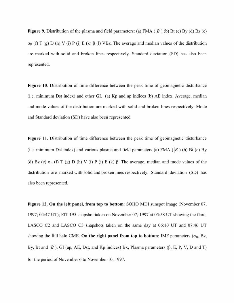
Figure 9. Distribution of the plasma and field parameters: (a) FMA ( B ) (b) Bt (c) By (d) Bz (e)

σB (f) T (g) D (h) V (i) P (j) E (k) β (l) VBz. The average and median values of the distribution

are marked with solid and broken lines respectively. Standard deviation (SD) has also been

represented.

Figure 10. Distribution of time difference between the peak time of geomagnetic disturbance

(i.e. minimum Dst index) and other GI. (a) Kp and ap indices (b) AE index. Average, median

and mode values of the distribution are marked with solid and broken lines respectively. Mode

and Standard deviation (SD) have also been represented.

Figure 11. Distribution of time difference between the peak time of geomagnetic disturbance

(i.e. minimum Dst index) and various plasma and field parameters (a) FMA ( B ) (b) Bt (c) By

(d) Bz (e) σB (f) T (g) D (h) V (i) P (j) E (k) β. The average, median and mode values of the

distribution are marked with solid and broken lines respectively. Standard deviation (SD) has

also been represented.

Figure 12. On the left panel, from top to bottom: SOHO MDI sunspot image (November 07,

1997; 04:47 UT); EIT 195 snapshot taken on November 07, 1997 at 05:58 UT showing the flare;

LASCO C2 and LASCO C3 snapshots taken on the same day at 06:10 UT and 07:46 UT

showing the full halo CME. On the right panel from top to bottom: IMF parameters (σB, Bz,

By, Bt and B ), GI (ap, AE, Dst, and Kp indices) Bx, Plasma parameters (β, E, P, V, D and T)

for the period of November 6 to November 10, 1997.

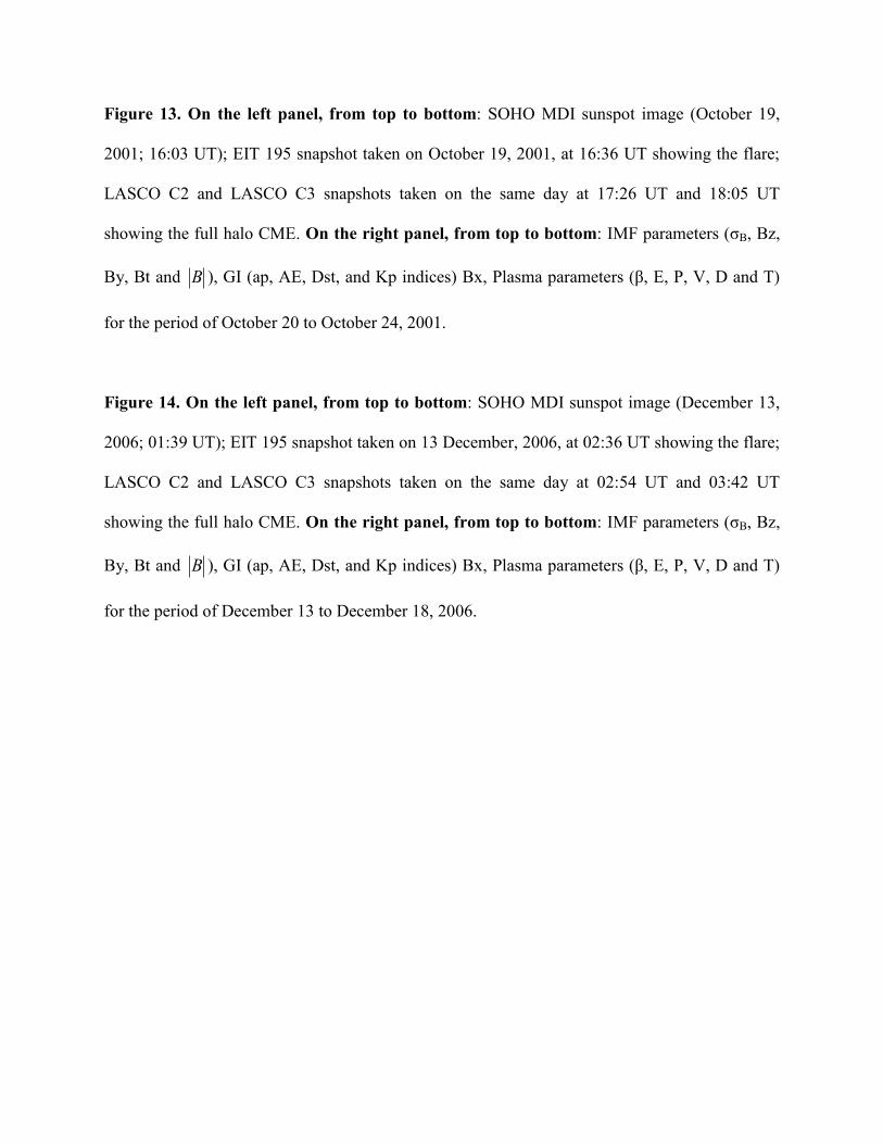
Figure 13. On the left panel, from top to bottom: SOHO MDI sunspot image (October 19,

2001; 16:03 UT); EIT 195 snapshot taken on October 19, 2001, at 16:36 UT showing the flare;


showing the full halo CME. On the right panel, from top to bottom: IMF parameters (σB, Bz,


for the period of October 20 to October 24, 2001.

Figure 14. On the left panel, from top to bottom: SOHO MDI sunspot image (December 13,

2006; 01:39 UT); EIT 195 snapshot taken on 13 December, 2006, at 02:36 UT showing the flare;


showing the full halo CME. On the right panel, from top to bottom: IMF parameters (σB, Bz,


for the period of December 13 to December 18, 2006.

Documents

BEHAVIOR OF PLASMA AND FIELD PARAMETERS AND THEIR