Behavioral Hazard in Health Insurance⇤

Katherine BaickerHarvard University

Sendhil MullainathanHarvard University

Joshua SchwartzsteinDartmouth College

March 25, 2015

Abstract

A fundamental implication of economic models of health insurance is that insurees overuselow-value medical care because the copay is lower than cost, i.e., because of moral hazard.There is ample evidence, though, that people misuse care for a different reason: behavioralerrors. For example, many highly beneficial drugs end up being under-used; and some uselesscare is bought even when the price equals cost. We refer to this kind of misuse as “behav-ioral hazard” and its presence changes the welfare calculus. With only moral hazard, demandelasticities alone can be used to make welfare statements, a fact many empirical papers relyon. In the presence of behavioral hazard, welfare statements derived only from the demandcurve can be off by orders of magnitude and can even be of the wrong sign. Highly elasticdemand suggests increasing copays when the care is low-value but suggests decreasing copayswhen the care is high-value. Making welfare statements requires knowing the health responseas well as the demand elasticity. We derive optimal copay formulas when both moral and be-havioral hazard can be present, providing a theoretical foundation for value-based insurancedesign. Our framework also provides a way to interpret behavioral interventions (“nudges”),suggests different implications for market equilibrium, and shows how health insurance doesnot just provide financial protection, but can also create incentives for more efficient treatmentdecisions.

⇤We thank Dan Benjamin, David Cutler, John Friedman, Drew Fudenberg, Ben Handel, Ted O’Donoghue, MatthewRabin, Jesse Shapiro, Andrei Shleifer, Jonathan Skinner, Chris Snyder, Douglas Staiger, Glen Weyl, Heidi Williams,Danny Yagan, and the anonymous referees for helpful comments. Schwartzstein thanks National Institute on Aging,Grant Number T32-AG000186 for financial support.

1 Introduction

Moral hazard is central to how we understand health insurance. Because the insured pay less forhealth care than it costs, they may overuse it (Arrow 1963; Pauly 1968; Zeckhauser 1970; Cutlerand Zeckhauser 2000). One feature of the standard moral hazard model has proven especiallyimportant for empirical analysis and policy work: the demand curve alone is enough to quantify theinefficiency generated by insurance (see Finkelstein 2014 for a review). When looking at a changein copays, we can draw welfare conclusions without ever measuring the health impacts because weinfer such impacts: if people optimize perfectly, health benefits equal copays at the margin. A largebody of empirical work relies on this “sufficient statistic” property to derive welfare calculationsand make policy recommendations (Newhouse 1993; Manning et al. 1987; Feldstein 1973). Yet,when it comes to health care choices, people may fail to optimize so perfectly. In this paper, wedevelop a richer model of health insurance that allows people to make mistakes and suggest thatrelying on the demand data alone can lead to highly misleading welfare calculations and optimalcopay prescriptions.

Many important health care choices are hard to reconcile with a world in which moral haz-ard alone drives misutilization. First, there are many examples of people underusing rather thanoverusing care, such as patients failing to use care whose health benefits substantially exceed costs(even accounting for possible side-effects or other non-monetary costs). Diabetes medications, forexample, have clear and large benefits—they increase life span, reduce the risk of limb loss orblindness, and improve the quality of life. Yet people fail to take them consistently: adherencerates for these medications is estimated at only 65% (Bailey and Kodack 2011). Diabetes is not theexception: we see low adherence for beneficial medications that help manage chronic conditions,as well as for treatments such as prenatal and post-transplant care (van Dulmen et al. 2007; Oster-berg and Blaschke 2005).1 Second, even when people over-use care, moral hazard is not alwaysthe reason: patients sometimes demand care that does not benefit at them or at times even harmsthem. For example, patients seek out antibiotics with clear risks and unclear benefits for oftenself-limiting conditions such as ear infections (Spiro et al. 2006). It is hard to explain this kind ofoveruse with a model based on private benefits exceeding private costs.

This evidence is consistent with a simple narrative. People do not misuse care only because the1In principle, it is possible to argue that unobserved costs of care, such as side effects, drive what seems to be

underuse. However, in practice, this argument is difficult to make for many of the examples we review. The underusewe focus on is very different from the underuse that can arise in dynamic moral hazard models. In such models,patients may underuse preventive care that generates monetary savings for the insurer (Goldman and Philipson 2007;Ellis and Manning 2007). Here, we focus on the underuse of care whose benefits outweigh costs to the consumer. Forexample, though the underuse of diabetes medications does generate future health care costs, the uninsurable privatecosts to the consumer alone (e.g. higher mortality and blindness) make non-adherence likely to be a bad choice evenif she is fully insured against future health care costs. We also abstract from underuse due to health externalities (e.g.the effect of vaccination on the spread of disease).

1

price is below the social marginal cost: they also misuse it because of behavioral biases—becausethey make mistakes. We call this kind of misutilization behavioral hazard. Many psychologiescontribute to behavioral hazard. People may overweight salient symptoms such as back pain orunderweight non-salient ones such as high blood pressure or high blood sugar. They may bepresent-biased (Newhouse 2006) and overweight the immediate costs of care, such as copays andhassle-costs of setting up appointments or filling prescriptions. They may simply forget to taketheir medications or refill their prescriptions. Or they may have false beliefs about the efficacy ofcare (Pauly and Blavin 2008). Section 2 introduces a model of behavioral hazard that nests suchbehavioral biases, as well as others within a large class.2

Behavioral hazard means that welfare calculations can no longer be made from demand dataalone. Consider the “marginal” insurees—those who respond to a copay change. In the standardmodel, these consumers are trading off the health benefits against the copay. Because they areperfectly optimizing, their indifference means the health benefits must roughly equal the copay.3

But Section 3 shows that with behavioral hazard this inference fails exactly because insurees maybe misvaluing care. For example, we would not want to falsely conclude that diabetes medicationsare ineffective because a modest copay reduces adherence (e.g., Lohr et al. 1986), or that breastcancer patients place little value on conserving their breasts because a modest copay induces themto switch from equally-effective breast-conserving lumpectomy to breast-removing mastectomy(e.g., Einav, Finkelstein, and Williams 2015).4 In these cases, the care is likely very effective:behavioral hazard means agents can be marginal in their choices even when the health benefits aremuch larger than the copay.

Empirical work suggests that this is more than an abstract concern. First, we look at caseswhere we understand the health benefits. Instead of seeing that low-value care is highly elasticand high-value care is inelastic, we find very similar elasticities for both. Second, we reexam-ine the results of a large-scale field experiment that eliminated copays for certain drugs for recentheart attack victims (Choudhry et al. 2011). Looking only at the demand response—a substantialincrease in drug use–would suggest significant moral hazard. Looking at the health outcomes,

2Of course, differentiating between these biases could help in designing non-price or behavioral interventions,but our focus is largely on the role of more standard price levers. Chetty (2009a) proposes a model of salience andtaxation in a similar way: he derives empirically implementable formulas for the incidence and efficiency costs oftaxation that are robust across positive theories for why agents may fail to incorporate taxes into choice. Our approachmore closely follows that of Mullainathan, Schwartzstein, and Congdon (2012). More broadly, our analysis is in thespirit of the “sufficient statistics” approach to public finance (Chetty 2009b), which develops formulas for the welfareconsequences of various policies that are functions of reduced-form elasticities.

3Technically, we can only equate the marginal private utility benefit with the copay, but presumably much of thisbenefit derives from the health effects.

4Indeed, there is evidence that providing decision aids to inform breast cancer patients about the relevant trade-offsincreases demand for the less invasive option (Waljee et al. 2007). One possibility is that patients may start from afalse mental model that the more invasive procedure works better.

2

however, shows substantial reductions in mortality and improvements in health. Thus, while tradi-tional analysis implies a welfare cost, taking behavioral hazard into account implies a much largerwelfare gain.

The failure of the demand curve to serve as a sufficient statistic also has implications for theoptimal design of insurance. We show in Section 4 that the optimal copay formula now dependson both demand and health responses, not just the demand response (Zeckhauser 1970).5 Thisprovides a formal foundation for “value-based insurance design” proposals that argue for lowercost-sharing for higher value care (Chernew, Rosen, and Fendrick 2007; Liebman and Zeckhauser2008; and Chandra et al. 2010), and our model nests a more specific result of Pauly and Blavin(2008) that applies to the case of uninformed consumers. Perhaps surprisingly, we show that thehealth value of treatment should be taken into account even when behavioral hazard is unsystematicand averages to zero across the population, so long as it is variable. We further show that healthinsurance now does not just provide financial protection: it can also create incentives for moreefficient treatment decisions.

Because it has qualitatively different implications, factoring in behavioral hazard can have alarge effect. In Section 5 we compare the optimal copay to the copay a “neo-classical analyst” whoignores behavioral hazard would think is optimal. The neo-classical analyst underestimates theoptimal copay whenever behavioral hazard is systematically positive, driving people to overuse,and overestimates the optimal copay whenever behavioral hazard is systematically negative, driv-ing people to underuse.6 In fact, we show that when behavioral hazard is really positive or reallynegative, the situations where a neo-classical analyst believes that copays should be particularlylow are precisely those situations where copays should be particularly high and vice versa. Whenbehavioral hazard is extreme, the neo-classical optimal copay is exactly wrong.

In addition to changing the calculus around optimal copays, our framework also has im-plications for the optimal use of nudges (Thaler and Sunstein 2009)—such as defaults and re-minders—to mitigate overuse and underuse, as well as to calibrate the degree of behavioral hazard.Section 6 discusses this as well as other extensions of the basic analysis, including what we mightexpect the market to deliver in equilibrium. Proofs are in the Online Appendix, as are further modelextensions and a case study applying the model to treatment of hypertension. Section 7 concludeswith a brief discussion of directions for future work.

5Spinnewijn (2014) analyzes the optimal design of unemployment insurance when job-seekers have biased be-liefs and similarly predicts that policies implementing standard sufficient statistics formulas become suboptimal whenagents make errors.

6The idea that the optimal copay is below the neo-classical optimal copay when behavioral hazard drives sys-tematic underuse parallels findings on self-commitment devices for present-biased agents. For example, DellaVignaand Malmendier (2004) show that sophisticated present-biased agents value gym memberships that reduce the priceof going to the gym below the social marginal cost, since this reduction counteracts internalities that result from theoverweighting of immediate costs relative to long-term benefits.

3

2 A Model of Behavioral and Moral Hazard

2.1 Moral Hazard

We begin with a stylized model of health insurance. Consider an individual with wealth y. Insur-ance has price, or premium, P . When healthy, she has utility U(y�P ) if she buys insurance. Withprobability q 2 (0, 1), she can fall sick with a specific condition with varying degree of severity s

that is private information on the part of the individual. For example, individuals may be afflictedwith diabetes that varies in how much it debilitates. Assume s ⇠ F (s), where F has support onS = [s, s] ⇢ R+ and s < s. Assume further that F (s) has strictly positive density f(s) on S .Severity is measured in monetary terms so that when sick, absent treatment, the agent receivesutility U(y � P � s).

Treatment can lessen the impact of the disease. Treatment costs society c, and its benefit b(s; �)depends on severity, where � 2 R is a parameter that allows for heterogeneity across peoplein treatment benefits conditional on disease severity, and is also private information.7 The moresevere the disease, the greater the benefits: bs > 0. We assume b(0; �) = 0 for all � (the unaffectedget no benefit) and bs 1 (the treatment cannot make people better off than not having the disease).The benefits are put in monetary terms. It is efficient for some but not all of the sick to get treated:b(s; �) < c < b(s; �) for all �. We assume that the insured individual pays price or “copay” p

for treatment. Notice that while the copay implicitly depends on the disease and treatment, it isindependent of s and �; we assume that both disease severity and treatment benefits cannot becontracted over because the insurer cannot perfectly measure these variables. The interpretation isthat the copay is conditional on all information known to the insurer, but the individual may havesome residual private information.8 In this way, we nest the traditional moral hazard model. Aninsured individual who receives treatment for his disease gets utility U(y � P � s+ b(s; �)� p).

We evaluate insurance contracts from the perspective of a benevolent social planner rankingcontracts based on social welfare.9 Welfare as a function of the copay and the premium equals

7As standard in the literature, we implicitly assume that, without insurance, consumers would face the socialmarginal cost of treatment, which abstracts from another rationale for why insurance coverage can be welfare-improving even for risk-neutral consumers: when treatment suppliers have market power, subsidizing treatment canbring copays closer to the social marginal cost of care (Lakdawalla and Sood 2009).

8We focus on a single specific condition for presentational simplicity, but the analysis is qualitatively similar if theperson can fall sick with different conditions and the specific condition she falls sick with is observable and verifiableto the insurer, so the insurer can set different copays across conditions.

9We take the policy-maker’s welfare function as given. See Bernheim and Rangel (2009) for a discussion of achoice-based approach to recovering consistent welfare functions from inconsistent choice behavior. In effect, we areassuming in Bernheim and Rangel’s framework that there is some (unmodeled in our framework) ancillary conditionthat the policy-maker uses to infer a consistent preference for the agent and that the objective of the welfare problemis to maximize this preference.

4

expected utility:

W (p, P ) = (1� q)U(y � P ) + qE[U(y � P � s+m(p)(b� p))|sick], (1)

where m(p) 2 {0, 1} represents an individual’s demand for care at a given price and equals 1 if andonly if the person demands treatment. The first term is the utility if individuals do not get sick witha specific condition: they simply pay the premium. The second term is the utility if they do getsick: the expected utility (depending on disease severity and other stochastic parameters, describedin more detail below) which includes the loss due to being sick (�s) as well as the benefits of carenet of costs to individuals (b � p) for the times they choose to use care (m(p) = 1). We assumethat insurance must be self-funding: P = P (p) = M(p)(c � p), where M(p) = E[m(p)] equalsthe per-capita aggregate demand at a given copay. As a result, we can re-write welfare solely as afunction of the copay: with some abuse of notation, W (p) ⌘ W (p, P (p)).

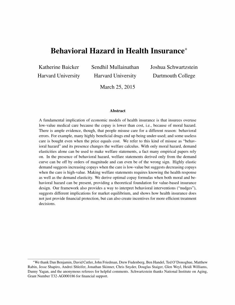
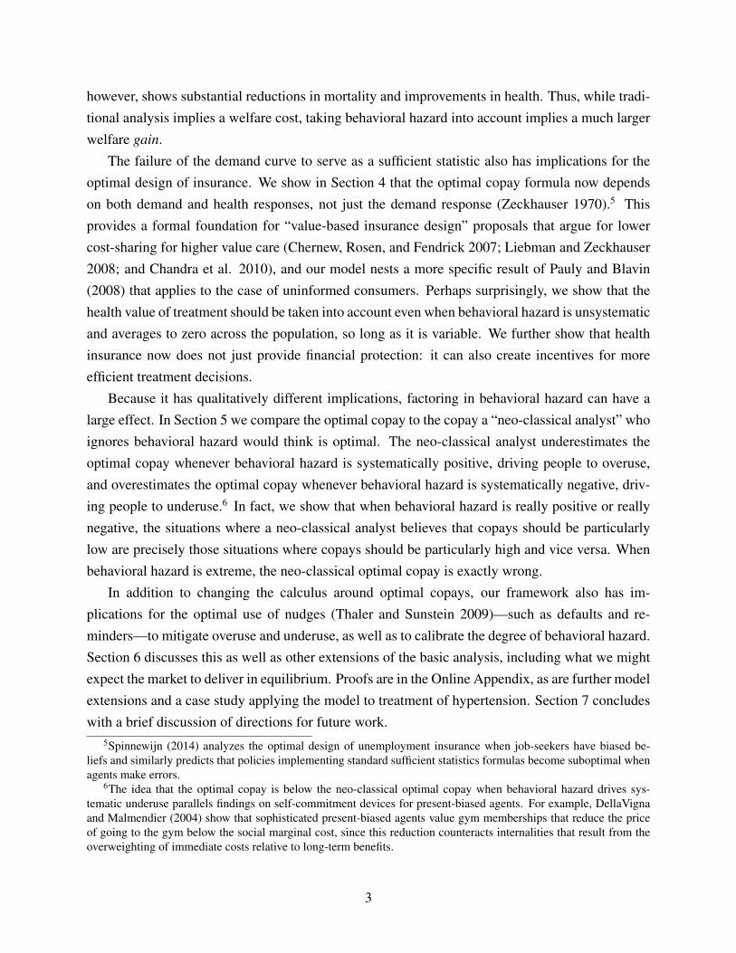
In this simple setup, the choice to receive treatment when insured is easy: the rational persongets treated whenever benefits exceed price, or b > p. This decision is the source of moral hazard.While the insurance value in insurance comes from setting price below true cost, or p < c, this sub-sidized price means that while individuals should efficiently get treated whenever b > c (benefitsexceed social costs), they get treated whenever b > p (benefits exceed private costs), generatinginefficient utilization when p < b < c . Figure 1 illustrates this. Individuals are arrayed on theline according to treatment benefits. Those to the right of the cost c should receive treatment anddo so. Those to the left of the price p should not receive treatment and do not. The middle regionrepresents the problem: those individuals should not receive treatment but they do. The price sub-sidy inherent to insurance is the source of misutilization: Raising the price individuals face woulddiminish overutilization, but come at the cost of diminished insurance value.10

2.2 Behavioral Hazard

There is, however, ample evidence of misutilization that is difficult to interpret as a rational per-son’s response to subsidized prices. We incorporate behavioral hazard through a simple modifica-tion of the original model. Instead of decisions being driven by a comparison of true benefits toprice, evaluating whether b(s; �) > p, people choose according to whether b(s; �) + "(s; ✓) > p,

where " is positive in the case of positive behavioral hazard (for example, seeking an ineffec-10For simplicity, we are assuming away income effects or issues of affordability. In a standard framework, insurance

could lead to more efficient decisions insofar as it makes high-value, high-cost procedures affordable to consumers(Nyman 1999). However, in this framework, insurance cannot lead consumers to make more efficient decisions on themargin. Abstracting from income effects serves to highlight this well-known fact (Zeckhauser 1970). Also, many ofthe examples we focus on involve low cost treatments such as prescription drugs where any income effects are likelyto be small.

5

Figure 1: Model with Only Moral Hazard

p c

b!"#$%!!$&'($)*! !$&'($)*!

!+"$,)-*!./0(1$! !./0(1$,!

2(3.%$!4!tive treatment for back pain) and negative in the case of negative behavioral hazard (for exam-ple, not adhering to effective diabetes treatment). The parameter ✓ 2 R allows for heterogene-ity across people in the degree of behavioral hazard and is not observable to the insurer. Weassume that b(s; �) + "(s; ✓) is differentiable and strictly increasing in s for all (�, ✓). The pa-rameters (�, ✓) are distributed independently from s, according to joint distribution G(�, ✓). Welet Q(s, �, ✓) = F (s)G(�, ✓) denote the joint distribution of all the possibly stochastic parame-ters. All expectations are taken with respect to this distribution unless otherwise noted. WhenU is non-linear, it will be useful to consider a “normalized” version of the behavioral error,"0(s; ✓) = U(y�P�s)�U(y�P�s�"(s;✓))

E[U 0(C)]

, which essentially puts " in utility units. (Note that " = "0

for linear U , so we have the approximation " ⇡ "0 if we take U to be approximately linear).This formulation builds on Mullainathan, Schwartzstein and Congdon (2012) and implicitly

captures a divide between preference as revealed by choice and utility as it is experienced, orbetween “decision utility” and “experienced utility” (Kahneman et al. 1997). In our frameworkb� p affects the experienced utility of taking the action. Individuals instead choose as if b+ "� p

affects this utility. We focus on behavioral models that imply a clear wedge between these twoobjects – in other words, models where people have a propensity to misbehave due to mistakes andfeature non-zero " terms, or “internalities”– rather than models of non-standard preferences.11

This simple formalization captures a variety of behavioral phenomena. Three examples arepresented here and summarized in Table 1: present-bias, symptom salience, and false beliefs.

Present-bias can be important because the benefits of medical care are often in the distantfuture while its costs appear now (Newhouse 2006). Take the canonical (�, �) model of present-bias (Laibson 1996, O’Donoghue and Rabin 1999), where, for simplicity, � = 1. Suppose eachtreatment is associated with an immediate cost but a delayed benefit. Specifically, b(s; �) =

11For example, anticipation and anxiety may alter how individuals experience benefits (Koszegi 2003): benefits willvary depending on whether taking the action (such as getting an HIV test) leads to anxiety in anticipating the outcome.In these kinds of situations it may be wrong to model the behavioral factor as a bias affecting ", but rather as a forcethat affects the mapping between outcomes (such as getting a diagnostic test) and benefits b.

6

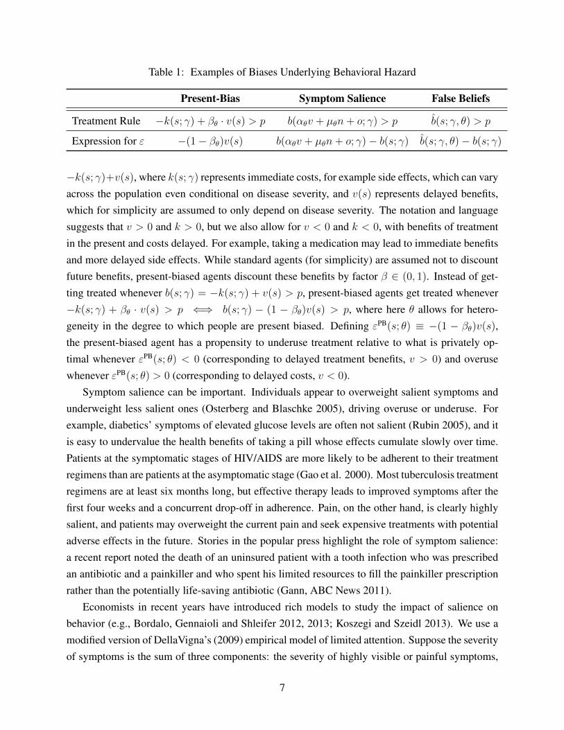
Table 1: Examples of Biases Underlying Behavioral Hazard

Present-Bias Symptom Salience False Beliefs

Treatment Rule �k(s; �) + �✓ · v(s) > p b(↵✓v + µ✓n+ o; �) > p b(s; �, ✓) > p

Expression for " �(1� �✓)v(s) b(↵✓v + µ✓n+ o; �)� b(s; �) b(s; �, ✓)� b(s; �)

�k(s; �)+v(s), where k(s; �) represents immediate costs, for example side effects, which can varyacross the population even conditional on disease severity, and v(s) represents delayed benefits,which for simplicity are assumed to only depend on disease severity. The notation and languagesuggests that v > 0 and k > 0, but we also allow for v < 0 and k < 0, with benefits of treatmentin the present and costs delayed. For example, taking a medication may lead to immediate benefitsand more delayed side effects. While standard agents (for simplicity) are assumed not to discountfuture benefits, present-biased agents discount these benefits by factor � 2 (0, 1). Instead of get-ting treated whenever b(s; �) = �k(s; �) + v(s) > p, present-biased agents get treated whenever�k(s; �) + �✓ · v(s) > p () b(s; �) � (1 � �✓)v(s) > p, where here ✓ allows for hetero-geneity in the degree to which people are present biased. Defining "PB(s; ✓) ⌘ �(1 � �✓)v(s),the present-biased agent has a propensity to underuse treatment relative to what is privately op-timal whenever "PB(s; ✓) < 0 (corresponding to delayed treatment benefits, v > 0) and overusewhenever "PB(s; ✓) > 0 (corresponding to delayed costs, v < 0).

Symptom salience can be important. Individuals appear to overweight salient symptoms andunderweight less salient ones (Osterberg and Blaschke 2005), driving overuse or underuse. Forexample, diabetics’ symptoms of elevated glucose levels are often not salient (Rubin 2005), and itis easy to undervalue the health benefits of taking a pill whose effects cumulate slowly over time.Patients at the symptomatic stages of HIV/AIDS are more likely to be adherent to their treatmentregimens than are patients at the asymptomatic stage (Gao et al. 2000). Most tuberculosis treatmentregimens are at least six months long, but effective therapy leads to improved symptoms after thefirst four weeks and a concurrent drop-off in adherence. Pain, on the other hand, is clearly highlysalient, and patients may overweight the current pain and seek expensive treatments with potentialadverse effects in the future. Stories in the popular press highlight the role of symptom salience:a recent report noted the death of an uninsured patient with a tooth infection who was prescribedan antibiotic and a painkiller and who spent his limited resources to fill the painkiller prescriptionrather than the potentially life-saving antibiotic (Gann, ABC News 2011).

Economists in recent years have introduced rich models to study the impact of salience onbehavior (e.g., Bordalo, Gennaioli and Shleifer 2012, 2013; Koszegi and Szeidl 2013). We use amodified version of DellaVigna’s (2009) empirical model of limited attention. Suppose the severityof symptoms is the sum of three components: the severity of highly visible or painful symptoms,

7

v, the severity of opaque or non-painful symptoms, n, and other symptoms, o, or

s = v + n+ o. (2)

The inattentive agent overweights the painful symptoms and underweights non-painful symptoms,so he acts not on true disease severity s, but on “decision severity”

s = ↵✓v + µ✓n+ o, (3)

where ↵✓ � 1 and �✓ 1. The magnitudes |1�↵✓| and |1�µ✓| can be thought of as parameterizingthe degree to which the agent misbehaves due to symptom salience, where he acts according to thestandard model when ↵✓ = µ✓ = 1. The person gets treated if

b(↵✓v + µ✓n+ o; �) > p () b(s; �) + [b(↵✓v + µ✓n+ o; �)� b(v + n+ o; �)] > p. (4)

Defining "SS(s; ✓) = b(↵✓v + µ✓n+ o; �)� b(v + n+ o; �), where we assume the right-hand-sideis constant in �, the person has a propensity to underuse treatment relative to what is privatelyoptimal whenever "SS(s; ✓) < 0, where non-painful symptoms are sufficiently prominent (i.e.,n > v(↵✓ � 1)/(1� µ✓) for µ✓ 6= 1), and has a propensity to overuse treatment relative to what isprivately optimal whenever "SS(s; ✓) > 0, where painful symptoms are sufficiently prominent (i.e.,v > n(1� µ✓)/(↵✓ � 1) for ↵✓ 6= 1).

False beliefs can also play a role (e.g., Pauly and Blavin 2008).12 Tuberculosis patients maystop taking their antibiotics halfway through their drug regimen not just because salient symptomshave abated, but also because they believe the disease has disappeared. People may falsely attributetreatment benefits as well, such as when they buy an herbal medicine with no known efficacy.13

Instead of getting treated when b(s; �) > p, agents with false beliefs get treated when b(s; �, ✓) >

p () b(s; �) + [b(s; �, ✓) � b(s; �)] > p, where b is the decision benefit to getting treated.Defining "FB(s; ✓) = b(s; �, ✓)�b(s; �), which for simplicity we assume is constant in �, the personwith false beliefs has a propensity to underuse treatment whenever "FB(s; ✓) < 0, where theyundervalue treatment (b(s; �, ✓) < b(s; �)), and has a propensity to overuse treatment whenever"FB(s; ✓) > 0, where they overvalue treatment (b(s; �, ✓) > b(s; �)).

12False beliefs may result from a variety of factors. Patients may have incomplete information; they may havefaulty mental models; they may not interpret evidence as Bayesians; they may be inattentive to available evidence.Section 6.1 highlights ways that distinguishing between such factors can be helpful, though we suspect that often acombination of factors are at play.

13Estimates suggest that the majority of antibiotics prescribed for adult respiratory infections were for conditionswhere an antibiotic would not be helpful, such as for a viral infection (Gonzales et al. 2001)—although, as discussedbelow, this may be attributable to a combination of patient and physician psychology.

8

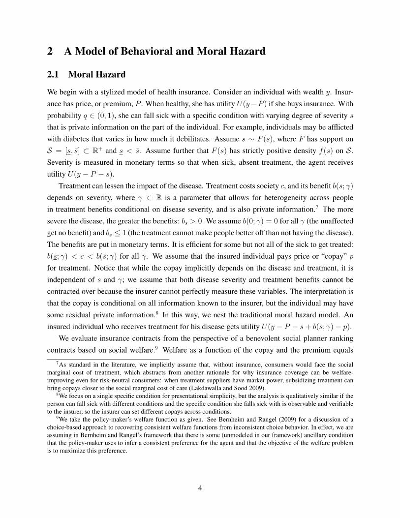
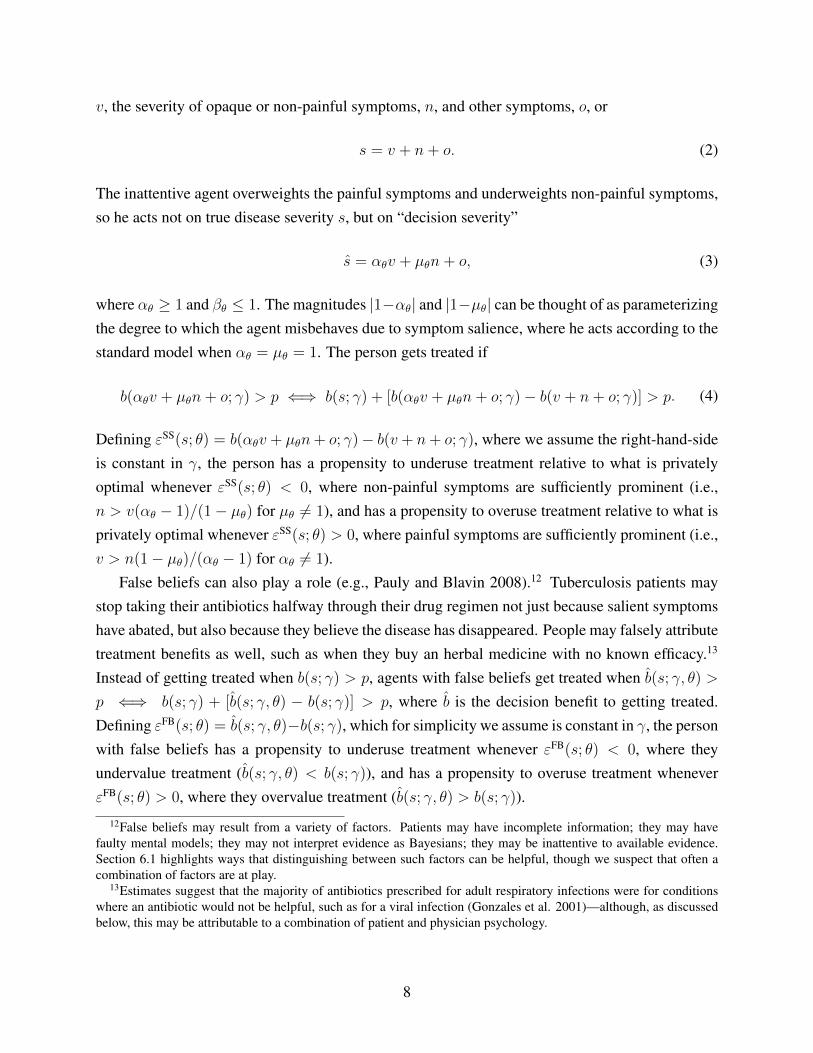
2.3 Misutilization with Behavioral Hazard

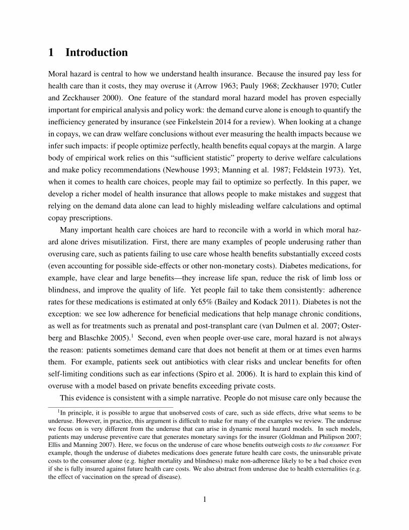
No matter the psychological micro-foundation, behavioral hazard changes how we think about thedemand for treatment. We illustrate this in Figure 2. We have now added a second axis to form asquare instead of an interval, where the vertical axis represents b+", which can vary by individual.The horizontal line separates the region where b+" > p, while the vertical line separates the regionwhere b > c. We see the ranges of misutilization are no longer clear. The people in the bottom leftcorner (where b + " < p and b < c) are efficient non-users. Those in the top right corner (whereb+ " > p and b > c) are efficient users. But there are now three other regions.

Figure 2: Model with Behavioral Hazard

b

b + !

c

p

!"#$%

&'(#$%

#)*+#',%

#)*+#',%

&-.+/#0%(!#0'1,%&-.+/#%

%02!&.('1,%&-.+/#%

%02!&.(%&-.+/#%

The bottom right area is a region of underutilization. People fail to consume care in thisregion because b + " < p, but the actual benefits exceed social cost. When there is behavioralhazard underutilization is a concern, not just overutilization due to moral hazard. Examples suchas the lack of adherence to drugs treating chronic conditions, like diabetes, hypertension, andhigh cholestorol, illustrate such underutilization, and Online Appendix Table 1 provides furtherexamples and references.14

14Underuse is of course not restricted to prescription drug non-adherence. Patients do not receive recommended careacross a wide range of categories, with only 55 percent receiving recommended preventive care including screenings(e.g., colonoscopies) and follow-up care for conditions ranging from diabetes and asthma management to post-hip-fracture care (McGlynn et al. 2003; Denberg et al. 2005; Ness et al. 2000).

9

The top left area illustrates overutilization. In this area, benefits of care are below cost so b < c,and the efficient outcome is for the individual not to get treated. Yet because b+ " > p the behav-ioral agent receives care. This area can be broken down further, according to whether b + " > c.When this inequality holds, decision benefits are above cost even though true benefits are belowcost. In this case, overutilization will not be solved by setting price at true cost. Examples suchas people demanding ineffective (or possibly harmful) antibiotics for sinus or ear infections, theovertreatment of prostate cancer, and the extremely high demand for MRIs for back pain may illus-trate such overutilization. Finally, the area of overutilization when b+ " c illustrates traditionaloverutilization due to moral hazard.

Misutilization is not solely a consequence of health insurance when there is behavioral hazard.Underuse, not just overuse, is a concern, and overuse may not be solved by setting prices at truecost. We next turn to the effects of these findings on the interpretation of observed elasticities andimplications for assessing welfare effects and optimal insurance design.

3 Moral Hazard Cannot be Inferred From the Demand CurveAlone

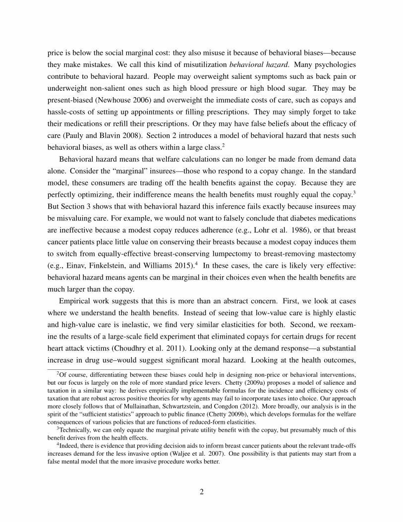
Behavioral hazard dramatically alters standard intuitions for how we think about the welfare impactof copay changes. Reducing a copay that is less than cost has two effects. Absent a demandresponse, it raises utility for people who are sick enough that they demand treatment, generatinginsurance value. Of course, people may choose to consume more care. The welfare impact of thisincrease depends on the magnitude and direction of behavioral hazard.

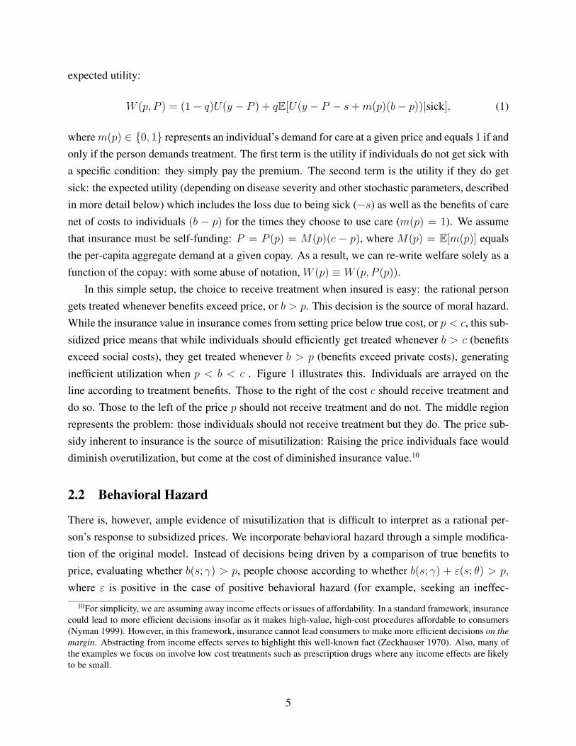
For a simple illustration, assume people are risk-neutral and consider the effect of reducing thecopay from cost (c) to zero in Panel (a) of Figure 3, which compares the welfare impact of thechange in utilization when there is only moral hazard to when there is also underuse from negativebehavioral hazard. The dark grey area represents the standard deadweight loss triangle — themoral hazard cost of insurance. This area is positive because people who get treated only when theprice is below marginal cost must have a willingness to pay below this cost. It is also greater theflatter the demand curve: more elastic demand means a greater moral hazard cost of insurance.

An often implicit assumption underlying the standard approach is that we can equate demandor willingness to pay with the true marginal benefit of treatment. Behavioral hazard drives a wedgebetween these objects. For example, Panel (a) illustrates the case where all people have a propen-sity to underuse because of negative behavioral hazard and share the same " < 0. In this case, themarginal benefit curve lies above the demand curve and the vertical difference equals |"|. When themagnitude of negative behavioral hazard (|"|) is sufficiently large, the marginal benefit of treatment

10

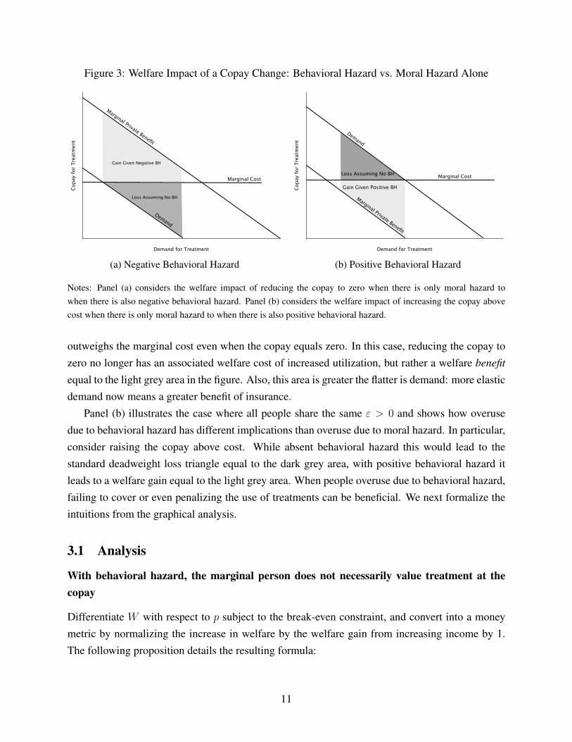
Figure 3: Welfare Impact of a Copay Change: Behavioral Hazard vs. Moral Hazard Alone

Demand for Treatment

Cop

ay f

or T

reat

men

t

Marginal Cost

Marginal Private Benefit

Demand

Gain Given Negative BH

Loss Assuming No BH

(a) Negative Behavioral Hazard

Demand for Treatment

Cop

ay f

or T

reat

men

t

Marginal Private Benefit

Demand

Marginal Cost

Gain Given Positive BH

Loss Assuming No BH

(b) Positive Behavioral Hazard

Notes: Panel (a) considers the welfare impact of reducing the copay to zero when there is only moral hazard towhen there is also negative behavioral hazard. Panel (b) considers the welfare impact of increasing the copay abovecost when there is only moral hazard to when there is also positive behavioral hazard.

outweighs the marginal cost even when the copay equals zero. In this case, reducing the copay tozero no longer has an associated welfare cost of increased utilization, but rather a welfare benefitequal to the light grey area in the figure. Also, this area is greater the flatter is demand: more elasticdemand now means a greater benefit of insurance.

Panel (b) illustrates the case where all people share the same " > 0 and shows how overusedue to behavioral hazard has different implications than overuse due to moral hazard. In particular,consider raising the copay above cost. While absent behavioral hazard this would lead to thestandard deadweight loss triangle equal to the dark grey area, with positive behavioral hazard itleads to a welfare gain equal to the light grey area. When people overuse due to behavioral hazard,failing to cover or even penalizing the use of treatments can be beneficial. We next formalize theintuitions from the graphical analysis.

3.1 Analysis

With behavioral hazard, the marginal person does not necessarily value treatment at thecopay

Differentiate W with respect to p subject to the break-even constraint, and convert into a moneymetric by normalizing the increase in welfare by the welfare gain from increasing income by 1.The following proposition details the resulting formula:

11

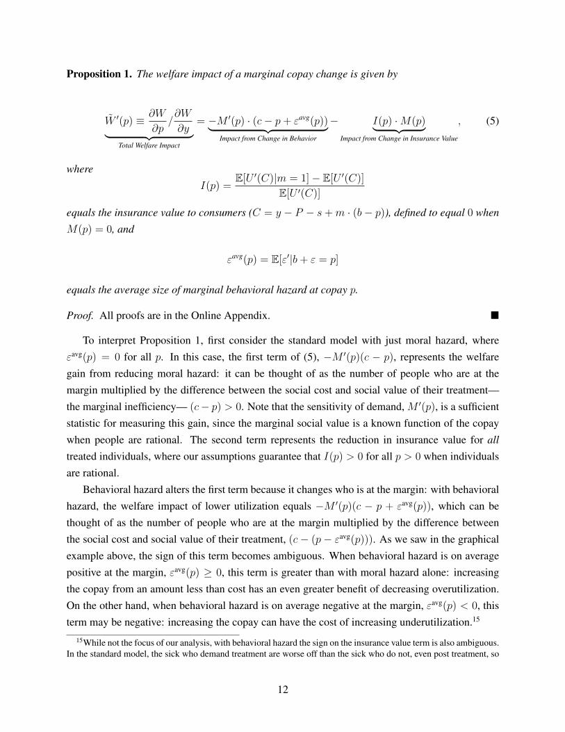
Proposition 1. The welfare impact of a marginal copay change is given by

W 0(p) ⌘ @W

@p/@W

@y| {z }Total Welfare Impact

= �M 0(p) · (c� p+ "avg(p))| {z }Impact from Change in Behavior

� I(p) ·M(p)| {z }Impact from Change in Insurance Value

, (5)

whereI(p) =

E[U 0(C)|m = 1]� E[U 0(C)]

E[U 0(C)]

equals the insurance value to consumers (C = y � P � s+m · (b� p)), defined to equal 0 whenM(p) = 0, and

"avg(p) = E["0|b+ " = p]

equals the average size of marginal behavioral hazard at copay p.

Proof. All proofs are in the Online Appendix. ⌅

To interpret Proposition 1, first consider the standard model with just moral hazard, where"avg(p) = 0 for all p. In this case, the first term of (5), �M 0(p)(c � p), represents the welfaregain from reducing moral hazard: it can be thought of as the number of people who are at themargin multiplied by the difference between the social cost and social value of their treatment—the marginal inefficiency— (c� p) > 0. Note that the sensitivity of demand, M 0(p), is a sufficientstatistic for measuring this gain, since the marginal social value is a known function of the copaywhen people are rational. The second term represents the reduction in insurance value for alltreated individuals, where our assumptions guarantee that I(p) > 0 for all p > 0 when individualsare rational.

Behavioral hazard alters the first term because it changes who is at the margin: with behavioralhazard, the welfare impact of lower utilization equals �M 0(p)(c � p + "avg(p)), which can bethought of as the number of people who are at the margin multiplied by the difference betweenthe social cost and social value of their treatment, (c� (p� "avg(p))). As we saw in the graphicalexample above, the sign of this term becomes ambiguous. When behavioral hazard is on averagepositive at the margin, "avg(p) � 0, this term is greater than with moral hazard alone: increasingthe copay from an amount less than cost has an even greater benefit of decreasing overutilization.On the other hand, when behavioral hazard is on average negative at the margin, "avg(p) < 0, thisterm may be negative: increasing the copay can have the cost of increasing underutilization.15

15While not the focus of our analysis, with behavioral hazard the sign on the insurance value term is also ambiguous.In the standard model, the sick who demand treatment are worse off than the sick who do not, even post treatment, so

12

Note that what matters for calculating the welfare impact of a marginal copay change is theaverage marginal size of behavioral hazard at copay p, "avg(p) = E["0|b + " = p], rather thanthe average unconditional size, E["0]. To see why, consider a situation where some people simplyforget to get treated (e.g. forget a prescription refill) with some probability �, but otherwise makean accurate cost-benefit calculation. In our framework, this can be captured by assuming that"(s; ✓) is very negative with probability � and otherwise equals zero. While the average degree ofbehavioral hazard in this example can be quite negative, behavioral hazard does not influence whois at the margin, since anyone who responds to a copay change is someone who makes an accuratecost-benefit calculation. Indeed, in this case the marginal degree of behavioral hazard is zero.

With behavioral hazard, demand responses do not measure the extent of moral hazard

Proposition 1 also formalizes the standard intuition that when there is merely moral hazard, theoverall demand response is a powerful tool for measuring the welfare impact of the changes inutilization driven by copay changes. Indeed, �M 0(p) · (c� p) is necessarily increasing in |M 0(p)|when p < c. But it shows that when there is behavioral hazard this composite response is harder tointerpret: looking at demand responses alone may provide a misleading impression, since �M 0(p)·(c � p + "avg(p)) is not necessarily increasing in |M 0(p)|. A high response might indicate a greatdeal of moral hazard (and hence a cost of providing insurance) or could indicate a great deal ofnegative behavioral hazard or price-responsive underutilization (and hence an additional benefit toinsurance).

In practice, researchers effectively ignore behavioral hazard by focusing on aggregate demandresponses in calculating the welfare impact of copay changes. For example, researchers calculateda welfare loss of $291 per person from moral hazard in 1984 dollars based on evidence from theRAND Health Insurance Experiment suggesting a demand elasticity of roughly -.2 (Manning etal. 1987; Feldman and Dowd 1991). While recent economic research has questioned whether sucha single elasticity can accurately summarize how people will respond to changes in non-linearhealth insurance contracts (Aron-Dine, Einav, and Finkelstein 2013), there has been less emphasison reexamining the basic assumption that the price sensitivity of demand meaningfully capturesthe degree of moral hazard. Indeed, in a recent review article of developments in the study ofmoral hazard in health insurance since Arrow’s (1963) original article, Finkelstein (2014) equatesevidence of moral hazard with evidence of the price sensitivity of demand for medical care.

A closer look at available evidence challenges this assumption. Table 2 summarizes evidenceindicating that demand for “effective care” is often as elastic as demand for “ineffective care”.

long as p > 0. Since this may not hold with behavioral hazard, stronger conditions (for example, that q is sufficientlysmall) are necessary to guarantee that the people who demand treatment on average have higher marginal utility thanthose who do not and consequently that I(p) > 0 for p > 0.

13

Analysis of the RAND health insurance experiment found that cost-sharing induced the same 40%reduction in demand for beta blockers as it did for cold remedies - with reductions for drugs deemed“essential” on average quite similar to those for drugs deemed “less essential” (Lohr et al. 1986).16

Goldman et al. (2006) estimate that a $10 increase in copayments drives similar reductions in useof cholestorol-lowering medications among those with high risk (and thus presumably those withhigh health benefits) as those with much lower risk. A quasi-experimental study of the effects ofsmall increases in copayments (rising from around $1 to around $8) among retirees in Californiaby Chandra, Gruber, and McKnight (2010) suggests that HMO enrollees’ elasticity for “lifestyledrugs” such as cold remedies and acne medication is virtually the same as for acute care drugssuch as anti-convulsants and critical disease management drugs such as beta-blockers and statins— all clustered around -0.15 (2007; unpublished details provided by authors). To take a partic-ularly striking example, which we discuss in greater detail below, relatively small reductions incopayments even after an event as salient as a heart attack still produce improvements in adher-ence (Choudhry et al. 2011). The evidence in fact suggests that the degree of moral hazard cannotbe inferred from aggregate demand responses.17

So how can we systematically distinguish between behavioral hazard and moral hazard? Onemethod is to measure health responses.

With behavioral hazard, measuring health responses helps identify who is at the margin

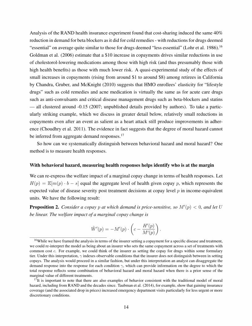
We can re-express the welfare impact of a marginal copay change in terms of health responses. LetH(p) = E[m(p) · b � s] equal the aggregate level of health given copay p, which represents theexpected value of disease severity post treatment decisions at copay level p in income-equivalentunits. We have the following result:

Proposition 2. Consider a copay p at which demand is price-sensitive, so M 0(p) < 0, and let Ube linear. The welfare impact of a marginal copay change is

W 0(p) = �M 0(p) ·✓c� H 0(p)

M 0(p)

◆.

16While we have framed the analysis in terms of the insurer setting a copayment for a specific disease and treatment,we could re-interpret the model as being about an insurer who sets the same copayment across a set of treatments withcommon cost c. For example, we could think of the insurer as setting the copay for drugs within some formularytier. Under this interpretation, � indexes observable conditions that the insurer does not distinguish between in settingcopays. The analysis would proceed in a similar fashion, but under this interpretation an analyst can disaggregate thedemand response into the response for each condition �, which can provide information on the degree to which thetotal response reflects some combination of behavioral hazard and moral hazard when there is a prior sense of themarginal value of different treatments.

17It is important to note that there are also examples of behavior consistent with the traditional model of moralhazard, including from RAND and the decades since. Taubman et al. (2014), for example, show that gaining insurancecoverage (and the associated drop in prices) increased emergency department visits particularly for less urgent or morediscretionary conditions.

14

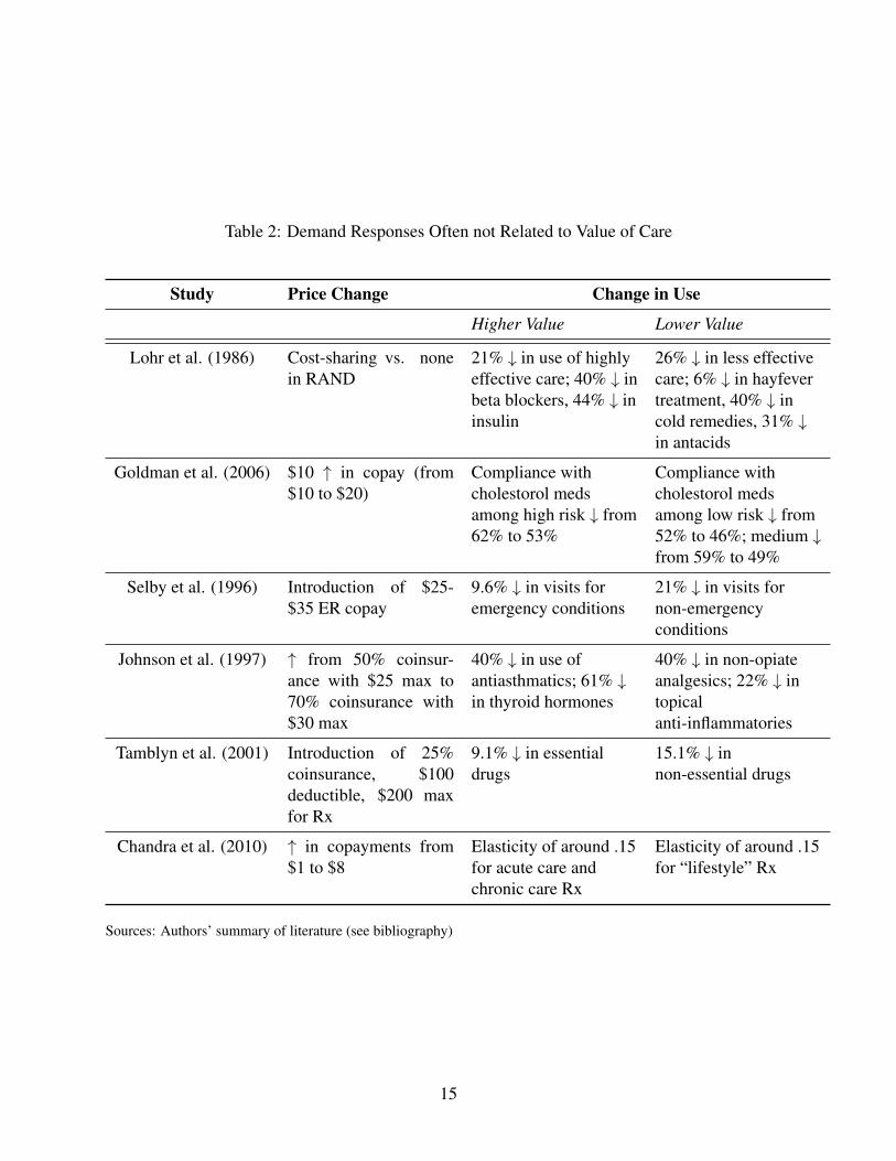
Table 2: Demand Responses Often not Related to Value of Care

Study Price Change Change in Use

Higher Value Lower Value

Lohr et al. (1986) Cost-sharing vs. nonein RAND

21% # in use of highlyeffective care; 40% # inbeta blockers, 44% # ininsulin

26% # in less effectivecare; 6% # in hayfevertreatment, 40% # incold remedies, 31% #in antacids

Goldman et al. (2006) $10 " in copay (from$10 to $20)

Compliance withcholestorol medsamong high risk # from62% to 53%

Compliance withcholestorol medsamong low risk # from52% to 46%; medium #from 59% to 49%

Selby et al. (1996) Introduction of $25-$35 ER copay

9.6% # in visits foremergency conditions

21% # in visits fornon-emergencyconditions

Johnson et al. (1997) " from 50% coinsur-ance with $25 max to70% coinsurance with$30 max

40% # in use ofantiasthmatics; 61% #in thyroid hormones

40% # in non-opiateanalgesics; 22% # intopicalanti-inflammatories

Tamblyn et al. (2001) Introduction of 25%coinsurance, $100deductible, $200 maxfor Rx

9.1% # in essentialdrugs

15.1% # innon-essential drugs

Chandra et al. (2010) " in copayments from$1 to $8

Elasticity of around .15for acute care andchronic care Rx

Elasticity of around .15for “lifestyle” Rx

Sources: Authors’ summary of literature (see bibliography)

15

Further, H 0(p)/M 0(p) = p if and only if "avg(p) = 0 and, more generally, "avg(p) = p �H 0(p)/M 0(p).

The first part of this proposition indicates that, all else equal, the welfare impact of a copayincrease inversely depends on the marginal health value of care.18 This is true not only when thereis behavioral hazard, but also in the rational model. Intuitively, a copay increase is less desirablewhen it discourages high-value care rather than low-value care. The second part clarifies whystandard formulas for the welfare impact of copay changes are not expressed in terms of healthresponses: absent behavioral hazard, we can equate the health response with the copay since beingmarginal reveals indifference. But it goes on to show that we cannot do this when there is thepossibility of marginal behavioral hazard: with behavioral hazard, we can no longer infer thehealth response from knowledge that someone is marginal. Rather, we can infer the degree ofmarginal behavioral hazard from the deviation between the copay and the marginal health value oftreatment.

In some of the cases described above, there are indications that the copay changes are asso-ciated with large health implications, providing further suggestive evidence for behavioral hazardin such cases. As summarized in Table 3, the copay increase studied by Chandra et al. (2010)was associated with an increase in subsequent hospitalizations and Hsu et al. (2006) similarly findthat the imposition of a cap on Medicare drug benefits lead to an greater nonelective hospital use.Choudhry et al. (2011) find that providing post-heart attack medications for free is associated witha reduced rate of subsequent major vascular events to an extent that, as we will discuss below, isinconsistent with plausible parameters under the standard model.

A challenge to using data on health responses to calibrate the degree of behavioral hazard isthat the health response may be difficult to observe or map to hedonic benefits. It may be possibleto estimate how much a pill reduces mortality risk and translate this into (money-metric) utility;it may be more difficult to estimate the unpleasantness of side-effects or the inconvenience oftreatment. In some instances, however, we may have enough information to confidently bound theunobservable component, in which case we can still say something about the sign and possibly themagnitude of behavioral hazard.19 This is more likely in the case of highly effective treatments

18The assumption of linear utility simplifies the presentation by allowing us to abstract from the insurance valueterm. It also simplifies the relationship between "avg(p) and H 0(p)/M 0(p). Otherwise, "avg(p) ⇡ p � H 0(p)/M 0(p)when U is approximately linear.

19To illustrate, decompose the change in health per marginal change in demand into observable and unobservablecomponents:

H 0(p)

M 0(p)= hO(p) + hU (p),

where hO(p) represents the observable component, and hU (p) the unobservable component. For example, the observ-able component could include a proxy for quality-adjusted life years gained per marginal filled prescription and theunobservable component could include non-pecuniary costs (e.g., side-effects) associated with filling the prescription

16

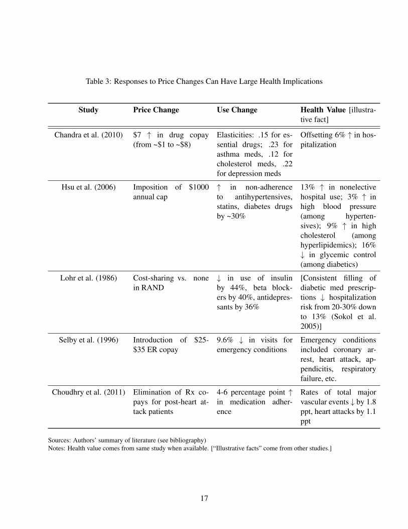
Table 3: Responses to Price Changes Can Have Large Health Implications

Study Price Change Use Change Health Value [illustra-tive fact]

Chandra et al. (2010) $7 " in drug copay(from ~$1 to ~$8)

Elasticities: .15 for es-sential drugs; .23 forasthma meds, .12 forcholesterol meds, .22for depression meds

Offsetting 6% " in hos-pitalization

Hsu et al. (2006) Imposition of $1000annual cap

" in non-adherenceto antihypertensives,statins, diabetes drugsby ~30%

13% " in nonelectivehospital use; 3% " inhigh blood pressure(among hyperten-sives); 9% " in highcholesterol (amonghyperlipidemics); 16%# in glycemic control(among diabetics)

Lohr et al. (1986) Cost-sharing vs. nonein RAND

# in use of insulinby 44%, beta block-ers by 40%, antidepres-sants by 36%

[Consistent filling ofdiabetic med prescrip-tions # hospitalizationrisk from 20-30% downto 13% (Sokol et al.2005)]

Selby et al. (1996) Introduction of $25-$35 ER copay

9.6% # in visits foremergency conditions

Emergency conditionsincluded coronary ar-rest, heart attack, ap-pendicitis, respiratoryfailure, etc.

Choudhry et al. (2011) Elimination of Rx co-pays for post-heart at-tack patients

4-6 percentage point "in medication adher-ence

Rates of total majorvascular events # by 1.8ppt, heart attacks by 1.1ppt

Sources: Authors’ summary of literature (see bibliography)Notes: Health value comes from same study when available. [“Illustrative facts” come from other studies.]

17

with few side effects than in treatments with non-pecuniary costs that may be experienced quitedifferently across people (e.g., colonoscopies). Section 6 shows that good prior knowledge ofthe psychology underlying behavioral hazard can help estimate the marginal degree of behavioralhazard in the latter situations.

3.2 An Illustration

We illustrate the potential magnitude of the importance of taking behavioral hazard into accountby further drawing on Choudhry et al.’s (2011) work on the effects of eliminating copays for recentheart attack victims.20 They randomly assigned patients discharged after heart attacks to a controlgroup with usual coverage (with copayments in the $12-$20 range) or a treatment group with nocopayments for statins, beta blockers, and ACE inhibitors (drugs of known efficacy), and trackedadherence rates and clinical outcomes over the next year. Faced with lower prices, consumers usedmore drugs: the full coverage group was significantly more adherent to their medications, using onaverage $106 more worth of cardiovascular-specific prescription drugs.

Under the moral hazard model, this fact alone tells us the health consequences of eliminatingcopays. Rational patients forgo only care with marginal value less than their out-of-pocket price.The average patient share under usual coverage in the Choudry data is about 25%, implying thatthe extra care consumed when copays are eliminated has a monetized health value of at most $.25on the dollar. Given the $106 increase in spending, the moral hazard model then predicts a healthimpact of at most $106 · .25 = $26.50 per patient. This in turn implies a moral hazard welfare lossfrom eliminating copayments of at least $106(1 � .25) = $79.50 per person. In other words, the$106 increase in spending is comprised of $26.50 of health value plus $79.50 of excess utilization.This is the kind of exercise routinely performed with demand data.21

But Choudhry et al. collected data on health impacts, which we can use to gauge the perfor-mance of the moral hazard model by comparing the implied health benefits with the observed ones.The increase in prescription drug use was associated with significantly improved clinical outcomes:

(all in dollars). If we can bound the unobservable component as belonging to [hU (p),hU (p)], then we can also boundthe extent of behavioral hazard:

"avg(p) 2 [p� (hO(p) + hU (p)), p� (hO(p) + hU (p))].

20We use this particular study because it measures not only demand responses, but also a rich variety of healthresponses. While the setting is admittedly quite specific, we believe the qualitative conclusions are illustrative forbroader populations and treatments. Online Appendix C provides a stylized example using the case study of treatmentfor high blood pressure, though it is difficult to perform a rigorous analysis given data limitations.

21Given the assumption that people have linear demand curves, we can derive a tighter lower bound on the welfareloss under the standard model. In this case, the moral hazard model implies a welfare loss of at least $106(1�.25/2) =$92.75 (see, e.g., Feldman and Dowd 1991).

18

patients in the full coverage group had lower rates of vascular events (1.8 percentage points), my-ocardial infarction (1.1 percentage points), and death from cardiovascular causes (.3 percentagepoints). We apply the commonly used estimate of a $1 million value of a statistical life to thereduction in the mortality to get a crude measure of the dollar value of health improvements.22

This implies that the elimination of copays leading to a .3 percentage point reduction in mortalitygenerates a value of $3,000. This $3,000 improvement substantially exceeds the standard model’sprediction of $26.50, suggesting large negative behavioral hazard. Applying the traditional moralhazard calculus in this situation implies that people place an unrealistically low valuation on theirlife and health.23

For welfare calculations, the theoretical analysis above highlights the need to use an estimateof the marginal private health benefit in the presence of behavioral hazard. As a rough back-of-the-envelope calculation, the $3,000 improvement in mortality minus the $106 increase in spendinggenerates a surplus of $2,894 per person (a gross return of $28 per dollar spent). The presence ofbehavioral hazard thus reverses how we interpret the demand response to eliminating copayments:moral hazard implies a welfare loss, while behavioral hazard implies a gain that is over 30 timeslarger.24

4 Implications for Optimal Copays

We have seen that behavioral hazard can influence whether changing copays from existing levelsis good policy. This section describes some features of the optimal plan when behavioral hazard istaken into account.

Consider again Equation (5), which gives us the welfare impact of a marginal copay increase.Setting this equal to zero yields a candidate for the optimal copay. To limit the number of cases,we focus attention on the standard situation where some but not all sick people are treated at the

22This calculation is admittedly crude, but provides an illustrative example. Estimates of the value of a statisticallife clearly vary based on the age at which death is averted and the life expectancy gained – averting the death of ayoung healthy worker might be valued at $5 million - and mortality is only one aspect of the potential changes inhealth. While the estimated reduction in mortality is not statistically significant at conventional levels, the other healthimpacts are. We focus on the mortality reduction because it is easiest to monetize in this illustration.

23It seems unlikely that the cost of unobserved side-effects of statins, beta blockers, and ACE-inhibitors is anywherenear $2894 for a given patient in a year, so taking these effects into account should not reverse the conclusion thateliminating copayments leads to a welfare gain.

24As in basic moral hazard calculations, this analysis ignores substitution between treatments. In this example,total spending (prescription drug plus nondrug) went down by a small, non-statistically significant amount whencopayments were eliminated on preventive medications after heart attack, as did insurer costs. Taking these non-significant offset effects at face value would imply that welfare goes up even before taking behavioral hazard intoaccount (Glazer and McGuire 2012), though it raises a puzzle as to why private insurers did not reduce copays on theirown. However, even in this case, incorporating behavioral hazard substantially changes the analysis by providing amuch stronger rationale for reducing the copay. More generally, evidence suggests that reducing copays on high-valuecare does not generate cost savings over short (1-3 year) horizons (Lee et al. 2013).

19

optimum: an optimal copay pB satisfies M 0(pB) < 0 and M(pB) > 0. This is true under ourassumptions, for example, when people are not too risk averse, i.e., when �U 00/U 0 is sufficientlysmall over the relevant range of C. For presentational simplicity, we also focus on the situationwhere the optimal copay is unique. Defining pmin = inf {p : M(p) < q} to equal the lowest copaywhere not every sick person demands treatment and pmax = sup {p : M(p) > 0} to equal thehighest copay where some sick person demands treatment, we assume the following.

Assumption 1. The optimal copay is unique and satisfies pB 2 (pmin, pmax).

Proposition 3. Assuming pB 6= 0, the optimal copay satisfies

c� pB

pB=

I

⌘� "avg

pB, (6)

where ⌘ = �M 0(p)p/M(p) equals the elasticity of demand for treatment, I the insurance value,and "avg the average size of marginal behavioral hazard, all evaluated at pB.

Proposition 3 expresses the optimal copay in terms of reduced-form elasticities as well as thedegree of behavioral hazard and the curvature of the utility function. It says that, fixing insurancevalue and the cost of treatment, the optimal copay is increasing in the demand elasticity and thedegree to which behavioral hazard is positive. This simple formula illustrates a number of ways inwhich behavioral hazard fundamentally changes how we think about optimal copays.

Optimal copays can substantially deviate from cost even when coverage generates little or noinsurance value

A simple implication of Equation (6) is that health “insurance” can provide more than financialprotection: it can lead to more efficient health delivery. Even when individuals are risk-neutral andthere is no value to financial insurance (I = 0), Equation (6) indicates that the optimal copay candiffer from cost to provide insurees with incentives for more efficient utilization decisions. In fact,when consumers are risk-neutral, the extent of behavioral hazard (at the margin) fully determinesthe optimal copay. In this case, the optimal copay formula reduces to pB = c + "avg(pB): theoptimal copay acts like a Pigouvian tax to induce the marginal insuree to fully internalize their“internality”. Unlike in the standard model, there is no clear incentive-insurance tradeoff.

Optimal copays can be extreme: It can be optimal to fully cover treatments that are ineffec-tive for some insurees or to deny coverage of treatments that benefit insurees

A related implication is that optimal copays can be more extreme than in a model with only moralhazard. Absent behavioral hazard, the optimal copay strictly lies between the value that provides

20

full insurance (i.e., the value that makes I(p) = 0) and cost when insurees are risk averse and de-mand is elastic. Intuitively, without behavioral hazard, slightly raising the copay from the amountthat provides full insurance has only a second order cost through reducing insurance value but afirst order benefit through controlling moral hazard; slightly reducing the copay from cost has asecond order cost through inducing moral hazard but a first order benefit through increasing insur-ance value. In the standard model, it cannot be optimal to deny coverage of treatments that benefitsome risk averse individuals and it cannot be optimal to fully cover or subsidize treatments whenpeople are price-sensitive at the full coverage copay.

Behavioral hazard alters these prescriptions. When behavioral hazard is sufficiently positive,the optimal copay can be above cost even when the individual is risk-averse: it can be good tolet insurers discriminate against certain treatments, as suggested by Panel (b) of Figure 3. Whenbehavioral hazard is sufficiently negative, the optimal copay can be below the level that providesfull financial protection, even if demand is price-sensitive at this copay: paying people to get treatedcan be optimal, as illustrated in Panel (a) of Figure 3. In this spirit, some insurers have begun toexperiment with paying patients to take their medications (Belluck 2010; Volpp et al. 2009).

Optimal copays depend on health value, not just demand elasticities

Optimal copays likely vary more across treatments than in a model with only moral hazard. Thestandard model says that, fixing insurance value, copays should be higher the larger the cost andelasticity of demand (Zeckhauser 1970), as can be seen from plugging "avg = 0 into Equation(6). That model suggests, for example, that copays should be lower for emergency care (wheredemand is less elastic) than for regular doctor’s office visits (where it is presumably more pricesensitive). However, it also leads to some counterintuitive prescriptions: It suggests that copaysshould be similar across broad categories of drugs with similar price elasticities, even if they havevery different efficacies.

Behavioral hazard alters these prescriptions as well. To see this, make the approximation"(s; ✓) ⇡ "0(s; ✓) 8 (s, ✓) and plug "avg(p) ⇡ p � H 0(p)/M 0(p) (Proposition 2 establishes thatthe second approximation follows from the first) into (6), yielding

c� pB

pB⇡ I

⌘+

✓H 0(pB)

pBM 0(pB)� 1

◆. (7)

From Equation (7), all else equal copays should be decreasing in the net return to the last privatedollar spent on treatment, |H 0(p)| / (p |M 0(p)|) � 1, so the value of treatment now enters into thedetermination of the optimal copay insofar as it influences H 0(p). For a given demand response tocopays, copays should be lower when this demand response has greater adverse effects on health.

21

This connects to value-based insurance design proposals (Chernew, Rosen and Fendrick 2007)where, all else equal, cost sharing should be lower for higher value care. While the marginal ratherthan the average value of care appears in Equation (7), knowledge of the average health value ofcare can provide a useful signal about the marginal health value. Consider a case where the de-mand curve slopes down only because of behavioral hazard: V ar(") > 0, but V ar(b) = 0. Thenthe marginal individual at any copay where demand is price-sensitive must have a marginal healthvalue equal to the average value b, which also can be expressed as (H(pmin)�H(pmax))/(M(pmin)�M(pmax)). (Recall that pmin equals the lowest copay where some of the sick do not demand treat-ment and pmax equals the largest copay where some people still demand treatment.) Generalizingthis example to allow for heterogeneity in private benefits in addition to heterogeneity in behavioralhazard yields the following result.

Proposition 4. Assume U is linear, M 0(c) 6= 0, and the distribution Q(s, ✓, �) is such that b(s; �)and "(s; ✓) are independently distributed according to symmetric and quasiconcave densities withV ar(") > 0.

1. pB > c if H(pmin

)�H(pmax

)

M(pmin

)�M(pmax

)

< c and E["] � 0.

2. pB = c if H(pmin

)�H(pmax

)

M(pmin

)�M(pmax

)

= c and E["] = 0.

3. pB < c if H(pmin

)�H(pmax

)

M(pmin

)�M(pmax

)

> c and E["] 0.

This shows that with behavioral hazard, the average value of care provides a useful signal forthe optimal copay. So long as there is some variability in behavioral hazard across people andbehavioral hazard does not systematically push people to privately overuse high-value treatmentsor privately underuse low-value treatments, then the optimal copay is above cost whenever thetreatment is not socially beneficial on average and is below cost whenever the treatment is sociallybeneficial on average. Take the case where E["] = 0. The average value of care signals the expecteddirection of behavioral hazard at the margin, since—as is familiar from standard signal-extractionarguments—the marginal patient’s expected valuation lies between the copay (his “revealed” val-uation if there is no behavioral hazard) and the unconditional average valuation (his valuation ifbeing marginal was independent of true valuation).25 The marginal degree of behavioral hazardis then negative at copays below the expected value of treatment and positive at copays above theexpected value of treatment. To illustrate, returning to the example where V ar(b) = 0 we have

25The assumptions that b and " are independently distributed according to symmetric and non-degenerate quasicon-cave distributions guarantee that E[b|b + " = p] lies in between p and E[b] (see, e.g., Chambers and Healy 2012).In a different context, Spinnewijn (2014) similarly shows that even when people make mean-zero errors in decidingwhether to purchase insurance (which are independent of true insurance value), a selection argument implies that thedemand curve systematically overestimates the insurance value for the insured and systematically underestimates theinsurance value for the uninsured.

22

that the marginal degree of behavioral hazard satisfies b + " = p ) " = p � b, which clearly isnegative if and only if the copay is below the expected value of treatment.

These results suggest that optimal copays should depend on the value of treatment in additionto the demand response. For example, we might expect that we should have high copays forprocedures that are not recommended but sought by the patient nonetheless and low copays insituations where people have asymptomatic chronic diseases for which there are effective drugregimens. While advocated by some health researchers—for example, Chernew et al. (2007)—such differential cost-sharing is a rarity in practice; we return to some possible reasons in Section6 below.

5 The Pitfalls of Ignoring Behavioral Hazard

Behavioral hazard modifies the central insights of the standard model. The goal of this section isto give a sense of how important it is to take behavioral hazard into account – how wrong wouldthe analyst be if he ignored behavioral hazard?

While the optimal copay, pB, satisfies W 0(pB) = 0, where W is defined in Equation (5), acandidate for the “neo-classical optimal copay”, pN , satisfies the following condition.

Definition 1. pN is a candidate for the neo-classical optimal copay when

@WN(pN)/@p ⌘ �M 0(p) · (c� p)� I(p) ·M(p) = 0

and (i) @WN/@p � 0 in a left neighborhood of pN , (ii) @WN/@p 0 in a right neighborhoodof pN , and (iii) at least one of the inequalities in (i) or (ii) is strict for some p in the relevantneighborhoods.

In other words, pN is a copay that an analyst applying the standard model to estimates of thedemand and insurance value schedules, (M(·), I(·)), thinks could be optimal. The neo-classicaloptimal and true optimal copays will clearly coincide when "(s; ✓) = 0 8 s, ✓. The direction of thedeviation between these copays is also intuitive. As established in Online Appendix A, there is awelfare benefit to raising the copay from the neo-classical optimum whenever behavioral hazard ison average positive for people at the margin, and there is a welfare benefit to reducing the copayfrom the neo-classical optimum whenever behavioral hazard is on average negative for people atthe margin.26 Less obvious, the deviation between the neoclassical optimal and true optimal copayscan be huge:

26A somewhat more subtle point can be seen by focusing on the case where behavioral hazard is either systematicallypositive or negative, meaning that "(s; ✓) (weakly) shares the same sign across (s, ✓). In this context, Proposition 6in Online Appendix A implies that optimal copays exceed the neo-classical optimal copay so long as some marginalindividuals exhibit positive behavioral hazard, as in this case "avg(p) > 0, and is below the neo-classical optimal copay

23

Proposition 5. Suppose U is strictly concave, "(s; ✓) = " 2 R , and b(s; �) = s 8 (s, �, ✓).

1. If " is sufficiently large then the neo-classical analyst believes pN = 0 is a candidate for theoptimal copay but the optimal copay in fact satisfies pB � c.

2. If " is sufficiently low then the neo-classical analyst believes pN = c is a candidate for theoptimal copay but the optimal copay in fact satisfies pB 0.

When behavioral hazard is extreme, the neo-classical optimal copay is exactly wrong: thesituations in which the neo-classical analyst believes that copays should be really low are preciselythose situations where copays should be really high and vice versa.27 In the case of very positivebehavioral hazard, almost everybody gets treated at p ⇡ c, so the neo-classical analyst thinksthere is no benefit to controlling moral hazard but there is an insurance value to reducing copays,suggesting to him an optimal copay of at most zero. In reality, however, many people who demandtreatment at p = c are inefficiently doing so, yielding a large benefit to controlling behavioralhazard by raising the copay above cost. So long as people are not extremely risk averse, a copayabove cost is better than any copay below cost. In the case of very negative behavioral hazard,almost nobody gets treated at p ⇡ c, so the neo-classical analyst sees a huge benefit to controllingmoral hazard since nobody appears to value the treatment as much as it costs. So long as peopleare not extremely risk averse, the neo-classical analyst believes the copay should roughly equalcost. In reality, however, even at a copay of zero, people at the margin of getting treated have abenefit above cost. There is no benefit to controlling behavior by raising the copay above zero, butthere is an insurance value cost, making the optimal copay at most zero.

An immediate corollary of Proposition 5 is the following:

Corollary 1. Suppose U is strictly concave, b(s; �) = s, "(s; ✓) = " 2 R 8 (s, �, ✓), and

" =

8<

:e with ex ante probability ⇢ 2 (0, 1)

�e with ex ante probability 1� ⇢.

so long as some marginal individuals exhibit negative behavioral hazard. Consider the case of positive behavioralhazard. Increasing the copay by a small amount from p = pN has the welfare benefit of counteracting the behavioralhazard of some individuals, and the welfare cost of raising the copay above the optimum for people who behaveaccording to the standard model. This result says that the welfare benefit of counteracting behavioral hazard winsout. The intuition, similar to that in O’Donoghue and Rabin’s (2006) analysis of optimal sin taxes, is that since pN isthe optimal copay for standard agents, any small change from p = pN only has a second-order cost on their welfare.On the other hand, since people with positive behavioral hazard are inefficiently using too much care at p = pN , asmall reduction in the amount of care they receive has a first-order welfare benefit. While the presence of people whobehave according to the standard model can impact the magnitude of the deviation between the optimal copay and theneo-classical optimum, it does not influence the direction of this deviation.

27Strict concavity matters for this result. With linear utility the neo-classical analyst believes pN = c is a candidatefor the optimal copay, independent of ". The assumption that b(s; �) = s simplifies matters by guaranteeing that thereis always a non-negative candidate for the neo-classical optimal copay because it implies that a zero copay (rather thana negative one) maximizes insurance value when all the sick are treated.

24

For sufficiently large e: pB � c or pB 0, where (i) pB � c if pN = 0 (but not pN = c) is acandidate for the neo-classical optimal copay and (ii) pB 0 if pN = c (but not pN = 0) is acandidate for the neo-classical optimal copay.

This corollary essentially restates Proposition 5 to say that when behavioral hazard is extreme,knowing that the neo-classical analyst believes that the copay should be very low signals that itshould be very high and knowing that he believes the copay should be very high signals that itshould be very low. For example, when the neo-classical optimal copay is 0, i.e. full insurance, theoptimal copay is above c, i.e., no insurance.28

For a numerical illustration, take the case where utility is quadratic, s is uniformly distributed,getting treated returns a person to full health, and the degree of behavioral hazard is constant acrossthe population. Table 4 details a resulting calculation for parameter values described in the notes.This example highlights several points. First, pB > pN whenever behavioral hazard is positive,and pB < pN whenever behavioral hazard is negative. Second, the optimal copay pB is increasingin ". Third, the neo-classical optimal copay pN is instead decreasing in ". Fourth, and as a result ofthe fact that pB and pN move in opposite directions as " moves away from 0, the deviation betweenpB and pN can be huge.29

These results illustrate that setting copays under the assumption that the demand responsesignals the degree of moral hazard leads to very wrong policy conclusions when behavioral haz-ard is extreme. The example of Choudhry et al. (2011) on eliminating copays for recent heartattack victims dramatically illustrates this for the case of negative behavioral hazard: given thesizable demand response to eliminating copayments for statins, beta blockers, and ACE inhibitors,a neo-classical analyst could mistakenly conclude that this is bad policy. There are also examplesconsistent with misreaction in the other direction, where the traditional model suggests low co-pays because insurees exhibit little price-sensitivity, while incorporating behavioral hazard might

28We can also see that when behavioral hazard is extreme, there is always a candidate for the neo-classical optimalcopay satisfying |pB � pN | � c: the degree to which the optimal copay can vary in response to behavioral hazard islarger than the degree to which the neo-classical optimal copay can vary in response to more standard considerations,like the elasticity of demand or the degree of risk aversion. Indeed, without behavioral hazard, the optimal copayalways lies in [0, c] under the assumption that b(s; �) = s.

29The case where " = 99 provides an illustrative example of the last point. This is a situation where there is a lot ofoveruse due to behavioral hazard, and patients are reasonably risk averse. The analyst who looks for behavioral hazardwill understand that copays should be really high to counteract overuse due to behavioral hazard: pB = 197.92, whichis well above the cost of treatment, c = 100. The neo-classical analyst who believes that everybody accurately tradesoff costs and benefits in making treatment decisions will observe that everybody gets treated when the price is lessthan or equal to 99 and half the population gets treated when the price is 299/2. Since the cost of treatment is c = 100,it looks to the analyst like there is very little benefit to controlling moral hazard: almost everybody seems to value thetreatment at more than its cost, and the extremely small fraction who do not still seem to value the treatment at 99%of its cost. On the other hand, since people are risk averse, there is a benefit to reducing copays. In fact, the marginalinsurance benefit appears to exceed the marginal moral hazard cost at a copay of 99. Further, since the marginal moralhazard cost is zero at all lower copays (everybody is already getting treated), the neo-classical analyst believes thecopay should go all the way down to zero when in fact optimally it should be almost double the cost!

25

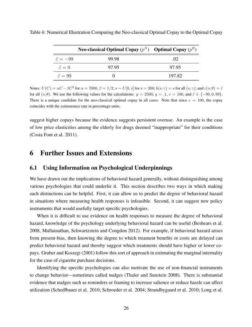
Table 4: Numerical Illustration Comparing the Neo-classical Optimal Copay to the Optimal Copay

Neo-classical Optimal Copay (pN ) Optimal Copay (pB)

" = �99 99.98 .02

" = 0 97.95 97.95

" = 99 0 197.82

Notes: U(C) = ↵C��C2 for ↵ = 7000,� = 1/2; s ⇠ U [0, s] for s = 200; b(s; �) = s for all (s, �); and "(s; ✓) = "

for all (s; ✓). We use the following values for the calculations: y = 2500, q = .1, c = 100, and " 2 {�99, 0, 99}.There is a unique candidate for the neo-classical optimal copay in all cases. Note that since c = 100, the copaycoincides with the coinsurance rate in percentage units.

suggest higher copays because the evidence suggests persistent overuse. An example is the caseof low price elasticities among the elderly for drugs deemed “inappropriate” for their conditions(Costa Font et al. 2011).

6 Further Issues and Extensions

6.1 Using Information on Psychological Underpinnings

We have drawn out the implications of behavioral hazard generally, without distinguishing amongvarious psychologies that could underlie it. This section describes two ways in which makingsuch distinctions can be helpful. First, it can allow us to predict the degree of behavioral hazardin situations where measuring health responses is infeasible. Second, it can suggest new policyinstruments that would usefully target specific psychologies.

When it is difficult to use evidence on health responses to measure the degree of behavioralhazard, knowledge of the psychology underlying behavioral hazard can be useful (Beshears et al.2008, Mullainathan, Schwartzstein and Congdon 2012). For example, if behavioral hazard arisesfrom present-bias, then knowing the degree to which treament benefits or costs are delayed canpredict behavioral hazard and thereby suggest which treatments should have higher or lower co-pays. Gruber and Koszegi (2001) follow this sort of approach in estimating the marginal internalityfor the case of cigarette purchase decisions.

Identifying the specific psychologies can also motivate the use of non-financial instrumentsto change behavior—sometimes called nudges (Thaler and Sunstein 2008). There is substantialevidence that nudges such as reminders or framing to increase salience or reduce hassle can affectutilization (Schedlbauer et al. 2010; Schroeder et al. 2004; Strandbygaard et al. 2010; Long et al.

26

2012).30 To incorporate such instruments into the framework, suppose there is a set N of nudgesavailable to the insurer, where a nudge is modeled as affecting demand through influencing thebehavioral error ", so for n 2 N , we have " = "n(s; ✓). The direct cost to the insurer of nudge n

is (n) � 0, where we suppose there is a “default nudge” n = 0 2 N with (0) = 0. So far wehave implicitly assumed that the insurer sets the default nudge and have notationally suppressedthe relationship between the nudge and the behavioral error.

Can we use responses to nudges to measure the magnitude of behavioral hazard? It is temptingto say that responses to reminders, for example, gauge the extent of inattention. But as Bordolo,Gennaioli and Shleifer (2015) point out, this inference may not be valid because people may over-react to such nudges. Nudges can be a useful tool for calibrating the degree of behavioral hazard,but only when we have a precise sense for how nudges affect the error—that is, how "n varies in n.For those cases, Proposition 7 in the Online Appendix describes conditions under which the degreeof marginal behavioral hazard can be calibrated by comparing the demand response to nudges tothe demand response to prices.31 Heuristically, if we find that a nudge believed to lead to betterdecisions increases demand for treatment more than a $d decrease in the copay, that suggests thatagents are undervaluing treatment by at least $d at the margin.32

It is difficult to perform this exercise rigorously with existing data because of the lack of studiesestimating the impact of nudges and copays simultaneously. However, the limited available evi-dence on the effects of nudges on adherence suggests that behavioral hazard can be significant. Forexample, Long et al. (2012) compare peer mentoring and financial incentives to improve glucosecontrol among African American veterans. While they do not measure impacts on drug adherence,they find that a peer mentoring program improved blood sugar control more than a $100-$200 in-centive did, which is suggestive of substantial negative behavioral hazard. (Also see Appendix Cfor evidence on the impact of nudges on hypertension.)

Nudges are also potentially useful policy tools for counteracting behavioral hazard when we30To illustrate, Schedlbauer et al. (2010) find that nudges focusing on reminders and reinforcements were particu-

larly promising ways to improve statin adherence, with four out of six trials reviewed producing significant increasesin adherence ranging from 6-24 percentage points. Similarly, simplifying the dosing schedules for blood pressuremedication can lead to a 10-20% increase in adherence (Schroeder et al. 2004).

31Chetty, Looney, and Kroft (2009) similarly describe conditions under which the marginal internality resultingfrom inattention to non-salient taxes can be recovered by comparing the demand response to taxes to the demandresponse to prices.

32It is not only important that the analyst have prior knowledge that the nudge leads to better decisions, but alsothat the nudge influences demand by impacting ". To illustrate, suppose people forget to demand treatment with someprobability � that may be dependent on nudges (e.g., reminders) but is independent of prices. If there are no otherbiases, then the marginal degree of behavioral hazard with respect to the price lever is zero, since anybody who ismarginal with respect to price is remembering and making an accurate cost-benefit calculation. However, we maystill see a sizable demand response to reminders. So, in this case, we cannot infer the marginal degree of behavioralhazard by comparing nudge and demand responses. Allcott and Taubinsky (2014) make a related point that analyzingthe demand response to nudges can give a misleading impression of the average marginal bias under certain forms ofheterogeneity in the bias across the population.

27

can be sure that they are reducing errors overall. A benefit of using nudges is that they can targetbehavioral hazard better than copays can. For example, if some fraction of the population exhibitsnegative behavioral hazard under the default nudge, "

0

(s; ✓) < 0 8s while some fraction actsunbiased, then there does not exist a copay that leads to first-best utilization: while p = c leadsto first-best utilization in the unbiased population, it leads to underuse among the people whoexhibit negative behavioral hazard. Further, while some p < c may potentially lead to efficientutilization in the population that exhibits negative behavioral hazard it leads to overuse amongthe people who are unbiased. On the other hand, if there is a “perfectly de-biasing nudge” n⇤

that eliminates behavioral hazard, "n⇤(s; ✓) = 0 8(s, ✓), then using that nudge leads to first-bestutilization when p = c.33 Of course, it is implausible that a perfectly de-biasing nudge exists.A cost of using certain nudges—at least for now—is that it is uncertain how effective they are atreducing behavioral hazard. Studying the optimal mix of nudges and copays in the design of healthinsurance, taking such uncertainty into account, is an interesting topic for future research.

6.2 Incorporating Testing Decisions

The existence of behavioral hazard can have ripple effects through other aspects of the deliverysystem, particularly if early utilization such as diagnostic testing has cascade effects for down-stream care. In the traditional model, the additional information yielded by low-cost tests shouldonly improve patient welfare, but with behavioral hazard, subsequent misbehavior can add largecosts. We briefly extend the model to allow for a testing stage which reveals s, and suppose theperson gets treated only if he is tested. To illustrate through a specific example, further supposethat U 00 = 0, s ⇠ U [0, 1], c = 3/4, and " = 3/4 for everybody. Without testing, nobody getstreated and welfare is E[�s] = �1/2 · q. With testing, everybody gets treated if p c, andwelfare equals �3/4 · q < �1/2 · q. So tests have a substantially negative return if behavioralhazard is uncontrolled (p = pN = c) and it is better not to test: the return on testing equals(�3/4 � (�1/2)) · q = (�1/4) · q. But it is better to test if behavioral hazard is controlled. Ifbehavioral hazard is perfectly counteracted (say, in this example, with copay pB = c + "), thentests would have a positive return: the return on testing is then (�15/32� (�1/2)) · q = (1/32) · q.So taking health responses into account in setting copays for treatment decisions can be doublybeneficial: not only does it lead to better decisions at the treatment stage, but it can feed back toresult in better policy at the testing stage.

The medical community has designed testing guidelines that implicitly acknowledge the im-33It is tempting to suppose that nudging in a way that eliminates errors is always optimal when such nudging

is possible and does not have direct costs. However, when people are risk averse then such debiasing can underminebroader social welfare in cases when it increases demand and, with it, the moral hazard cost of insurance (Mullainathan,Schwartzstein and Congdon 2012; Pauly and Blavin 2008).

28

perfections in the downstream decision-making of patients and physicians alike. The “ChoosingWisely” initiative launched by internal medicine physicians highlights common screenings andtests that they have blanket recommendations against, not because the tests themselves are cost-ineffective conditional on optimal downstream care, but explicitly because of the probability ofdownstream care that is likely to harm patient health but is delivered nonetheless (Morden et al.2014). These tests yield useful information that should be acted upon for only a subset of iden-tifiable patients, but many other patients end up receiving care (whether because of the disutilityof “doing nothing” or mistaken beliefs about efficacy) that is at best useless and at worst harmful,making the expected value of performing the test on anyone negative.34 This downstream sub-optimal care is of course the product of both patient and physician decision-making, and theremay be ample parallel opportunity to redesign physician incentives to take into account the psy-chology of their decision-making (as well as train them to help take into account the behavioraldecision-making of their patients).35 But if physician and patient behavioral hazard in subsequentcare decisions could be addressed, it would be efficient to conduct many of these tests.

6.3 Analyzing What the Market Will Provide

Given the welfare benefits of counteracting behavioral hazard, one question is why existing plansdo not seem to do so. As shown in Online Appendix Table 2, typical health insurance plans have acopay structure that varies little within broad categories of treatments (e.g., physician office visits,inpatient services, branded drugs, generic drugs), while counteracting behavioral hazard requiresa more nuanced structure where copayments are a function of the health benefit associated withthe care for a particular patient. In an earlier version of this paper (Baicker, Mullainathan andSchwartzstein 2013) we extend the model to consider what a competitive market will provide inequilibrium under the simplifying assumption of a representative insuree, which requires additionalassumptions on the degree to which insurees are sophisticated about behavioral hazard. We showhow even though optimal insurance could reduce behavioral hazard, market-provided insurancemay not. If enrollees are sophisticated, perfectly predicting their behavioral hazard and insuringaccordingly, then market-provided insurance would be optimally designed to counteract behavioralhazard. But with naive enrollees, insurers have less incentive to mitigate underuse since naiveconsumers will not fully value copays designed to counteract their biases.36 These problems are

34Ding et al. (2011) and others have calculated the economic costs associated with “incidental” findings —abnormalities detected in asymptomatic patients in the course of a separate evaulation.

35One study found, for example, that physicians’ propensity to prescribe contraindicated antibiotics for their patientsrose over the duration of their shift - a pattern attributed to physicians’ diminishing capacity to resist patient requestsfor prescriptions (Linder et al. 2014).

36Insurers will face some incentive to counteract negative behavioral hazard since naive consumers over-estimatetheir demand in this case, which creates some benefit to reducing copays. But, in general, negative behavioral haz-

29

especially severe when insurers have nudges as well as copays available and when they have limitedtime horizons (and thus do not bear the full cost of enrollees’ future health care use). In particular,if insurees do not appreciate the impact of nudges, then we would expect the insurer to supplynudges that minimize costs rather than maximize surplus.

These results suggest that when insurees are naive about their biases, then competitive forcesonly create incentives for the insurer to counteract biases when this saves the insurer money. Sincethe gains from reducing copays for antidiabetics, beta blockers and other negative behavioral haz-ard care may not accrue to the insurer, these results may shed light on why more health insur-ance plans do not incorporate behavioral hazard into their copayment structures.37 For example,Beaulieu et al. (2003) estimate that investment in diabetes disease management produces verysmall monetary gains for insurers over a 10 year horizon, but would produce $30,000 per patient inimproved quality of life and longevity.38 The potential for market failure suggests that governmentinterventions may be welfare-improving over market outcomes even in the absence of selectionor externalities.39 An important direction for future work is to develop a better understanding ofthe degree to which insurees are sophisticated about behavioral hazard in making insurance planchoices how the government could intervene to help counteract behavioral hazard.

7 Discussion

There is ample evidence that moral hazard alone cannot explain the patterns of misutilizationobserved throughout the health care system. We build a framework for analyzing the relationship

ard will not be efficiently managed in equilibirum. The discussion of market-provided insurance connects with theliterature on behavioral contract theory and industrial organization. Ellison (2006) and Spiegler (2011) provide nicereviews of this literature.

37Nevertheless, insurers could increase profits by promoting adherence to medications and treatments that savemoney over a reasonably short horizon (relative to the typical tenure of their enrollees), and the model suggests thatinsurers will invest in encouraging care in such instances. For example, flu shots are often given for free and at en-rollees’ convenience. Perhaps for a similar reason, insurers are also funding research into promoting adherence tocertain treatments (Belluck 2010) and in-house programs aimed at improving adherence, such as Humana’s “RxMen-tor” or United’s “Refill and Save” programs. Aetna’s tracking suggests that its program targeting chronic diseasepatients has improved adherence (Sipkoff 2009). FICO, known for its widely-purchased credit score, is now evenselling medication adherence scores to insurers, intended to predict how likely patients are to adhere (Parker-Pope2011).

38Additionally, while it could be efficient to provide negative prices (subsidies) to use high-value care (Volpp. et.al. 2009), practical considerations may make this infeasible. Current regulatory restrictions may also limit the abilityof insurers to counteract behavioral hazard. For example, there are limits to the ability of insurers to offer plans withdifferent copayments for the same drug to different patients, or for plans operating within Medicare to offer negativeprices (cash incentives) to enrollees.

39We abstract from ex ante heterogeneity among consumers and issues of selection. Of course, adverse selectionprovides a rationale for government intervention even in the standard model. Sandroni and Squintani (2007, 2010),Jeleva and Villeneuve (2004), and Spinnewijn (2013, 2014) explore how ex ante heterogeneity in risk perceptions oroverconfidence alter equilibrium insurance contracts, the relationship between risk and insurance coverage, and thewelfare impact of various government policies, e.g., insurance mandates.

30

between insurance coverage and health care consumption that also includes behavioral hazard.Incorporating behavioral hazard alongside moral hazard changes the fundamental tradeoff betweeninsurance and incentives. With only moral hazard, lowering copays increases the insurance valueof a plan but reduces its efficiency by generating overuse. With the addition of behavioral hazard,lowering copays may potentially both increase insurance value and increase efficiency by reducingunderuse. This means that having an estimate of the demand response is no longer enough to setoptimal copays; the health response needs to be considered as well. This provides a theoreticalfoundation for value-based insurance design, where copays should optimally be lower both whenprice changes have relatively small effects on demand and when they have relatively large effectson health. We show that ignoring behavioral hazard can lead to welfare estimates that are bothwrong in sign and off by an order of magnitude.

The framework developed is amenable to a number of extensions. While our model is static,it could be extended to consider how behavioral hazard affects optimal copays for preventive care,where initial underuse could generate high future costs (and possibly overuse). The New Eng-land Healthcare Institute estimates that eliminating non-adherence could save $290 billion a year.Further exploration of the sophistication of behavioral consumers and intertemporal incentives forinsurers may help explain the kinds of insurance plans we would expect to be provided in themarketplace and the potential role of public policy. Work could also draw out more nuanced im-plications for the use of nudges versus copayments. And while we highlight that the main resultsdo not depend on the underlying psychological forces generating behavioral hazard, greater under-standing of those forces could help estimate the degree of behavioral hazard in different settingsand inform the optimal design of nudges.

The finding that optimal insurance features depend crucially on how prices affect both quantitydemanded and health highlights the value of having empirical estimates of both demand responsesand health responses to changes in copays (see also Lee et al. 2013). There is often limited datalinking insurance and clinical outcomes—and performing an exhaustive list of experiments andcalculations would certainly be daunting—but a small number of conditions account for a largeshare of health spending. Patients with circulatory system conditions like high blood pressureand high cholesterol are responsible for 17% of total health care spending; mental conditionslike depression for another 9%; respiratory conditions like asthma another 6%; and endocrineconditions like diabetes another 4% (Roehrig et al. 2009). This means that a limited number ofstudies linking price changes, demand changes, and health changes could go a long way.40

40Even absent such multi-step evidence, however, we can glean some benchmarks about the potential benefits ofoptimal copayment design in a model with both moral hazard and behavioral hazard from the literature that looksat particular steps in this chain. This requires applying results from one particular step (e.g. the effect of a copaychange on one measure of adherence, such as refilling prescriptions) generated from a particular marginal populationto the next step (e.g. effect of a different measure of adherence, such as missed pills, on heart attacks) generated in

31

The model captures important features of the health care landscape. Many of the domains ofcare that are responsible for a substantial share of total health care utilization are sensitive to co-pay changes, and many of the treatments affected seem to have health value that differs from thatimplied by moral hazard alone. Failing to incorporate behavioral hazard into models of optimalinsurance design can not only generate very wrong answers – but very wrong answers with sub-stantial import for millions of people. The framework developed here builds a foundation for moresophisticated insurance design that incorporates both demand and health responses in balancinginsurance protection with efficient resource use.

ReferencesAllcott, Hunt and Dmitry Taubinsky, “The Lightbulb Paradox: Evidence from two Randomized Experi-

ments,” 2014.

Aron-Dine, Aviva, Liran Einav, and Amy Finkelstein, “The RAND Health Insurance Experiment, ThreeDecades Later,” Journal of Economic Perspectives, 2013, 27 (1), 197–222.

Arrow, Kenneth J, “Uncertainty and the Welfare Economics of Medical Care,” The American EconomicReview, 1963, pp. 941–973.

Baicker, Katherine, Sendhil Mullainathan, and Joshua Schwartzstein, “Behavioral Hazard in HealthInsurance,” 2013.

Bailey, CJ and Michael Kodack, “Patient Adherence to Medication Requirements for Therapy of Type 2Diabetes,” International Journal of Clinical Practice, 2011, 65 (3), 314–322.

Beaulieu, Nancy, David M Cutler, Katherine Ho, George Isham, Tammie Lindquist, Andrew Nel-son, and Patrick O’Connor, “The Business Case for Diabetes Disease Management for Managed CareOrganizations,” Frontiers in Health Policy Research, 2006, 9 (1), 1.

Belluck, Pam, “For Forgetful, Cash Helps the Medicine go Down,” The New York Times, 2010.

Bernheim, B Douglas and Antonio Rangel, “Beyond Revealed Preference: Choice-Theoretic Foundationsfor Behavioral Welfare Economics,” Quarterly Journal of Economics, 2009, 124 (1), 51–104.

a different setting with a different population, over a different time frame, etc. Appendix C provides a very stylizedexample using the case study of treatment for high blood pressure. High blood pressure afflicts 68 million adults inthe U.S. (CDC Vital Signs 2011) and is an important driver of overall health care costs. Using existing estimates, weshow that small reductions in copays increase compliance with anti-hypertensive therapy and that better compliancegenerates substantial health gains. This implies a large net return on the marginal social dollar spent on improvingblood-pressure medication adherence and suggests that the failure of existing plans to address behavioral hazard couldbe generating large welfare costs. Rosen et al. (2005) perform a similar exercise to predict the cost-effectiveness offirst-dollar coverage of ACE inhibitors for Medicare beneficiaries with diabetes.

32

Beshears, John, James J Choi, David Laibson, and Brigitte C Madrian, “How are Preferences Re-vealed?,” Journal of Public Economics, 2008, 92 (8), 1787–1794.

Bordalo, Pedro, Nicola Gennaioli, and Andrei Shleifer, “Salience Theory of Choice Under Risk,” TheQuarterly Journal of Economics, 2012, 1243, 1285.

, , and , “Salience and Consumer Choice,” Journal of Political Economy, 2013, 121 (5), 803–843.

, , and , “Memory, Attention, and Choice,” 2015.

CDC, “High Blood Pressure and Cholesterol,” National Center for Chronic Disease Prevention and HealthPromotion, 2011.

Chambers, Christopher P and Paul J Healy, “Updating toward the signal,” Economic Theory, 2012, 50(3), 765–786.

Chandra, Amitabh, Jonathan Gruber, and Robin McKnight, “Patient Cost-Sharing and HospitalizationOffsets in the Elderly,” The American Economic Review, 2010, 100 (1), 193.

Chernew, Michael E, Allison B Rosen, and A Mark Fendrick, “Value-Based Insurance Design,” HealthAffairs, 2007, 26 (2), w195–w203.

Chetty, Raj, “The Simple Economics of Salience and Taxation,” 2009.

, “Sufficient Statistics for Welfare Analysis: A Bridge Between Structural and Reduced-Form Methods,”Annual Review of Economics, 2009, 1 (1), 451–488.

, Adam Looney, and Kory Kroft, “Salience and Taxation: Theory and Evidence,” American EconomicReview, 2009, 99 (4), 1145–1177.

Choudhry, Niteesh K, Jerry Avorn, Robert J Glynn, Elliott M Antman, Sebastian Schneeweiss,Michele Toscano, Lonny Reisman, Joaquim Fernandes, Claire Spettell, Joy L Lee et al., “Full Cov-erage for Preventive Medications After Myocardial Infarction,” New England Journal of Medicine, 2011,365 (22), 2088–2097.

Cutler, David M and Richard J Zeckhauser, “The Anatomy of Health Insurance,” Handbook of HealthEconomics, 2000, 1, 563–643.

DellaVigna, Stefano, “Psychology and Economics: Evidence from the Field,” Journal of Economic Litera-ture, 2009, 47 (2), 315–372.

and Ulrike Malmendier, “Contract Design and Self-Control: Theory and Evidence,” The QuarterlyJournal of Economics, 2004, pp. 353–402.

33

Denberg, Thomas D, Trisha V Melhado, John M Coombes, Brenda L Beaty, Kenneth Berman, Tim EByers, Alfred C Marcus, John F Steiner, and Dennis J Ahnen, “Predictors of Nonadherence to Screen-ing Colonoscopy,” Journal of General Internal Medicine, 2005, 20 (11), 989–995.

Ding, Alexander, Jonathan D Eisenberg, and Pari V Pandharipande, “The Economic Burden of Inci-dentally Detected Findings,” Radiologic Clinics of North America, 2011, 49 (2), 257–265.

Einav, Liran, Amy Finkelstein, and Heidi Williams, “Paying on the Margin for Medical Care: Evidencefrom Breast Cancer Treatments.”

Ellis, Randall P and Willard G Manning, “Optimal Health Insurance for Prevention and Treatment,”Journal of Health Economics, 2007, 26 (6), 1128–1150.

Ellison, Glenn, “Bounded Rationality in Industrial Organization,” Econometric Society Monographs, 2006,42, 142.

Feldman, Roger and Bryan Dowd, “A New Estimate of the Welfare Loss of Excess Health Insurance,”The American Economic Review, 1991, pp. 297–301.

Feldstein, Martin S, “The Welfare Loss of Excess Health Insurance,” The Journal of Political Economy,1973, pp. 251–280.

Finkelstein, Amy, Moral Hazard in Health Insurance, Columbia University Press, 2014.

Font, Joan Costa and Marin Gemmill Toyama, “Does Cost Sharing Really Reduce Inappropriate Pre-scriptions Among the Elderly?,” Health Policy, 2011, 101 (2), 195–208.

Gann, Carrie, “Man Dies From Toothache, Couldn’t Afford Meds,” ABC News, 2011.

Gao, Xin, DP Nau, SA Rosenbluth, V Scott, and C Woodward, “The Relationship of Disease Severity,Health Beliefs and Medication Adherence Among HIV Patients,” AIDS Care, 2000, 12 (4), 387–398.

Glazer, Jacob and Thomas G McGuire, “A Welfare Measure of "Offset Effects" in Health Insurance,”Journal of Public Economics, 2012, 96 (5), 520–523.

Goldman, Dana and Tomas J Philipson, “Integrated Insurance Design in the Presence of Multiple MedicalTechnologies,” American Economic Review, 2007, 97 (2), 427–432.

Goldman, Dana P, Geoffrey F Joyce, Pinar Karaca-Mandic et al., “Varying Pharmacy Benefits withClinical Status: The Case of Cholesterol-Lowering Therapy,” American Journal of Managed Care, 2006,12 (1), 21.

Gonzales, Ralph, Daniel C Malone, Judith H Maselli, and Merle A Sande, “Excessive Antibiotic Use forAcute Respiratory Infections in the United States,” Clinical Infectious Diseases, 2001, 33 (6), 757–762.

34

Gruber, Jonathan and Botond Koszegi, “Is Addiction "Rational"? Theory and Evidence,” The QuarterlyJournal of Economics, 2001, 116 (4), 1261–1303.

Hsu, John, Mary Price, Jie Huang, Richard Brand, Vicki Fung, Rita Hui, Bruce Fireman, Joseph PNewhouse, and Joseph V Selby, “Unintended Consequences of Caps on Medicare Drug Benefits,” NewEngland Journal of Medicine, 2006, 354 (22), 2349–2359.

Jarvik, Jeffrey G, William Hollingworth, Brook Martin, Scott S Emerson, Darryl T Gray, StevenOverman, David Robinson, Thomas Staiger, Frank Wessbecher, Sean D Sullivan et al., “Rapid Mag-netic Resonance Imaging vs Radiographs for Patients with Low Back Pain: A Randomized ControlledTrial,” Journal of the American Medical Association, 2003, 289 (21), 2810–2818.

Jeleva, Meglena and Bertrand Villeneuve, “Insurance Contracts with Imprecise Probabilities and AdverseSelection,” Economic Theory, 2004, 23 (4), 777–794.

Johnson, Richard E, Michael J Goodman, Mark C Hornbrook, and Michael B Eldredge, “The Impactof Increasing Patient Prescription Drug Cost Sharing on Therapeutic Classes of Drugs Received and onthe Health Status of Elderly HMO Member,” Health Services Research, 1997, 32 (1), 103.

Kahneman, Daniel, Peter P Wakker, and Rakesh Sarin, “Back to Bentham? Explorations of ExperiencedUtility,” The Quarterly Journal of Economics, 1997, pp. 375–405.

Koszegi, Botond, “Health Anxiety and Patient Behavior,” Journal of Health Economics, 2003, 22 (6),1073–1084.

and Adam Szeidl, “A Model of Focusing in Economic Choice,” The Quarterly Journal of Economics,2012.

Laibson, David, “Golden Eggs and Hyperbolic Discounting,” The Quarterly Journal of Economics, 1997,pp. 443–477.

Lakdawalla, Darius and Neeraj Sood, “Innovation and the Welfare Effects of Public Drug Insurance,”Journal of Public Economics, 2009, 93 (3), 541–548.

Lee, Joy L, Matthew L Maciejewski, Shveta S Raju, William H Shrank, and Niteesh K Choudhry,“Value-Based Insurance Design: Quality Improvement but no Cost Savings,” Health Affairs, 2013, 32(7), 1251–1257.

Liebman, Jeffrey and Richard Zeckhauser, “Simple Humans, Complex Insurance, Subtle Subsidies,”2008.

Linder, Jeffrey A, Jason N Doctor, Mark W Friedberg, Harry Reyes Nieva, Caroline Birks, DaniellaMeeker, and Craig R Fox, “Time of Day and the Decision to Prescribe Antibiotics,” JAMA InternalMedicine, 2014, 174 (12), 2029–2031.

35

Lohr, Kathleen N, Robert H Brook, Caren J Kamberg, George A Goldberg, Arleen Leibowitz, JoanKeesey, David Reboussin, and Joseph P Newhouse, “Use of Medical Care in the RAND Health Insur-ance Experiment: Diagnosis-and Service-Specific Analyses in a Randomized Controlled Trial,” Medicalcare, 1986, pp. S1–S87.

Long, Judith A, Erica C Jahnle, Diane M Richardson, George Loewenstein, and Kevin G Volpp,“Peer Mentoring and Financial Incentives to Improve Glucose Control in African American Veterans: ARandomized Trial,” Annals of Internal Medicine, 2012, 156 (6), 416–424.

Manning, Willard G, Joseph P Newhouse, Naihua Duan, Emmett B Keeler, and Arleen Leibowitz,“Health Insurance and the Demand for Medical Care: Evidence from a Randomized Experiment,” TheAmerican Economic Review, 1987, pp. 251–277.

McGlynn, Elizabeth A, Steven M Asch, John Adams, Joan Keesey, Jennifer Hicks, Alison DeCristo-faro, and Eve A Kerr, “The Quality of Health Care Delivered to Adults in the United States,” NewEngland Journal of Medicine, 2003, 348 (26), 2635–2645.

Morden, Nancy E, Carrie H Colla, Thomas D Sequist, and Meredith B Rosenthal, “Choosing Wisely-The Politics and Economics of Labeling Low-Value Services,” New England Journal of Medicine, 2014,370 (7), 589–592.

Mullainathan, Sendhil, Joshua Schwartzstein, and William J Congdon, “A Reduced-Form Approach toBehavioral Public Finance,” Annual Review of Economics, 2012, 4.

Ness, Reid M, Ann M Holmes, Robert Klein, and Robert Dittus, “Cost-Utility of One-Time Colono-scopic Screening for Colorectal Cancer at Various Ages,” The American Journal of Gastroenterology,2000, 95 (7), 1800–1811.

Newhouse, Joseph P., Free for All?: Lessons from the RAND Health Insurance Experiment, Harvard Uni-versity Press, 1993.

Newhouse, Joseph P, “Reconsidering the Moral Hazard-Risk Avoidance Tradeoff,” Journal of Health Eco-nomics, 2006, 25 (5), 1005–1014.

Nyman, John A, “The Value of Health Insurance: The Access Motive,” Journal of Health Economics, 1999,18 (2), 141–152.

O’Donoghue, Ted and Matthew Rabin, “Doing it Now or Later,” American Economic Review, 1999,pp. 103–124.

and , “Optimal Sin Taxes,” Journal of Public Economics, 2006, 90 (10), 1825–1849.

Osterberg, Lars and Terrence Blaschke, “Adherence to Medication,” New England Journal of Medicine,2005, 353 (5), 487–497.

36

Parker-Pope, Tara, “Keeping Score on How You Take Your Medicine,” The New York Times, 2011.

Pauly, Mark V, “The Economics of Moral Hazard: Comment,” The American Economic Review, 1968,pp. 531–537.

and Fredric E Blavin, “Moral Hazard in Insurance, Value-Based Cost Sharing, and the Benefits ofBlissful Ignorance,” Journal of Health Economics, 2008, 27 (6), 1407–1417.

Roehrig, Charles, George Miller, Craig Lake, and Jenny Bryant, “National Health Spending by MedicalCondition, 1996–2005,” Health Affairs, 2009, 28 (2), w358–w367.

Rosen, Allison B, Mary Beth Hamel, Milton C Weinstein, David M Cutler, A Mark Fendrick, andSandeep Vijan, “Cost-Effectiveness of Full Medicare Coverage of Angiotensin-Converting Enzyme In-hibitors for Beneficiaries with Diabetes,” Annals of Internal Medicine, 2005, 143 (2), 89–99.

Rubin, Richard R, “Adherence to Pharmacologic Therapy in Patients with Type 2 Diabetes Mellitus,” TheAmerican Journal of Medicine, 2005, 118 (5), 27–34.

Sandroni, A and F Squintani, “Overconfidence and Adverse Selection: the Case of Insurance,” TechnicalReport, Working Paper 2010.

Sandroni, Alvaro and Francesco Squintani, “Overconfidence, Insurance, and Paternalism,” The AmericanEconomic Review, 2007, pp. 1994–2004.

Schedlbauer, Angela, Philippa Davies, and Tom Fahey, “Interventions to Improve Adherence to LipidLowering Medication,” 2010.

Schroeder, Knut, Tom Fahey, and Shah Ebrahim, “How Can We Improve Adherence to Blood Pressure–Lowering Medication in Ambulatory Care?: Systematic Review of Randomized Controlled Trials,”Archives of Internal Medicine, 2004, 164 (7), 722–732.

Selby, Joe V, Bruce H Fireman, and Bix E Swain, “Effect of a Copayment on Use of the EmergencyDepartment in a Health Maintenance Organization,” New England Journal of Medicine, 1996, 334 (10),635–642.

Sipkoff, Martin, “Improved Adherence Highlights Specialty Pharmacy’s Potential,” Managed Care, 2009,18 (10), 17.

Spiegler, Ran, Bounded Rationality and Industrial Organization, Oxford University Press, 2011.

Spinnewijn, Johannes, “Insurance and Perceptions: How to Screen Optimists and Pessimists,” The Eco-nomic Journal, 2013, 123 (569), 606–633.

, “Heterogeneity, Demand for Insurance and Adverse Selection,” 2014.

37

Spiro, David M, Khoon-Yen Tay, Donald H Arnold, James D Dziura, Mark D Baker, and Eugene DShapiro, “Wait-and-see Prescription for the Treatment of Acute Otitis Media: a Randomized ControlledTrial,” Journal of the American Medical Association, 2006, 296 (10), 1235–1241.

Strandbygaard, Ulla, Simon Francis Thomsen, and Vibeke Backer, “A Daily SMS Reminder IncreasesAdherence to Asthma Treatment: A Three-Month Follow-up Study,” Respiratory Medicine, 2010, 104(2), 166–171.

Tamblyn, Robyn, Rejean Laprise, James A Hanley, Michael Abrahamowicz, Susan Scott, NancyMayo, Jerry Hurley, Roland Grad, Eric Latimer, Robert Perreault et al., “Adverse Events Asso-ciated with Prescription Drug Cost-Sharing Among Poor and Elderly Persons,” Journal of the AmericanMedical Association, 2001, 285 (4), 421–429.

Taubman, Sarah L, Heidi L Allen, Bill J Wright, Katherine Baicker, and Amy N Finkelstein, “Med-icaid Increases Emergency-Department Use: Evidence from Oregon’s Health Insurance Experiment,”Science, 2014, 343 (6168), 263–268.

Thaler, Richard H and Cass R Sunstein, Nudge: Improving Decisions About Health, Wealth, and Happi-ness, Penguin, 2008.

van Dulmen, Sandra, Emmy Sluijs, Liset van Dijk, Denise de Ridder, Rob Heerdink, and Jozien Bens-ing, “Patient Adherence to Medical Treatment: A Review of Reviews,” BMC Health Services Research,2007, 7 (1), 55.

Volpp, Kevin G, Mark V Pauly, George Loewenstein, and David Bangsberg, “P4P4P: An Agenda forResearch on Pay-for-Performance for Patients,” Health Affairs, 2009, 28 (1), 206–214.

Waljee, Jennifer F, Mary AM Rogers, and Amy K Alderman, “Decision Aids and Breast Cancer: DoThey Influence Choice for Surgery and Knowledge of Treatment Options?,” Journal of Clinical Oncology,2007, 25 (9), 1067–1073.

Zeckhauser, Richard, “Medical Insurance: A Case Study of the Tradeoff Between Risk Spreading andAppropriate Incentives,” Journal of Economic Theory, 1970, 2 (1), 10–26.

38

Appendix (for Online Publication)

A Further Results

A.1 Comparing the Neo-classical Optimal Copay to the Optimal Copay

Proposition 6. Suppose the neo-classical analyst believes pN is a candidate for the optimal copaywhere M 0(pN) 6= 0.

1. W 0(pN) > 0 if "avg(pN) > 0. Moreover, pB > pN under the additional assumption thatW (p) is strictly quasi-concave over (pmin, pmax).

2. W 0(pN) < 0 if "avg(pN) < 0. Moreover, pB < pN under the additional assumption thatW (p) is strictly quasi-concave over (pmin, pmax).

This result says that there is a welfare benefit to raising the copay from the neo-classical op-timum whenever behavioral hazard is on average positive for people at the margin given this co-pay, and we further know that the optimal copay is above the neo-classical optimum wheneverW satisfies the classical regularity assumption of being strictly quasi-concave. Similarly, there is awelfare benefit to reducing the copay whenever behavioral hazard is on average negative for peopleat the margin, and the optimal copay is below the neo-classical optimum whenever W is strictlyquasi-concave. For example, the neo-classical analyst may underestimate the optimal copay in thecase of antibiotics for childrens’ ear infections but overestimate the optimal copay in the case ofstatins for people who have recently had a heart attack.

A.2 Using Nudges to Identify Behavioral Hazard

The next result describes conditions under which nudges can be used to help estimate the degreeof marginal behavioral hazard.

Proposition 7. Suppose that "n(s; ✓) is constant in ✓ and b(s; �) is constant in � for all (n, s).Let "n(p) = E["n|b + "n = p] equal the degree of marginal behavioral hazard given nudge n andcopay p.

1. (Negative behavioral hazard). Suppose we know that "0

0 and "n 0 for all s. Further,let p

0

, pn be such that p0

< pn, but 0 < M0

(p0

) Mn(pn) < q. Then,

�"0

(p0

) � pn � p0

. (8)

1

2. (Positive behavioral hazard). Alternatively, suppose we know that "0

� 0 and "n � 0 for alls. Further, let p

0

, pn be such that pn < p0

, but 0 < Mn(pn) M0

(p0

) < q. Then,

"0

(p0

) � p0

� pn. (9)

To illustrate how Proposition 7 can be used to estimate "0

, suppose a researcher is convincedthat a treatment is undervalued, and he has access to nudge n which he believes reduces behavioralhazard. Bound (8) can be applied whenever demand is interior and M

0

(p0

) Mn(pn). The lattercondition can be re-written as

Mn(p0)�M0

(p0

)| {z }demand response to nudge

� [Mn(p0)�Mn(pn)]| {z }demand response to co-pay change

� 0, (10)

so bound (8) can be applied whenever the demand response to an increase in copay from p0

topn, fixing the nudge at n, is lower in magnitude than the demand response to the nudge, fixing thecopay at p

0

. Thus, the tightest lower bound a researcher can estimate for �"0

(p0

) for a given nudgen is pn � p

0

, where pn is the value of pn that equates the demand response to an increase in copayto the demand response to the nudge; i.e., it is the value that makes (10) hold with equality.

Absent further assumptions, it is necessary to both have an estimate of the impact of a nudgeon demand as well as an estimate of demand sensitivity to copays under the nudge to directly applyEquation (10). For example, if the aim is to estimate the marginal behavioral error by examiningthe impact of a peer mentoring program on prescription drug utilization, Equation (10) requiresknowledge both of how the program affects utilization, fixing the copay, and how utilization re-sponds to greater copays when the program is in place. Under stronger assumptions, for examplethat demand is linear and demand sensitivity to copays is independent of the nudge, it is possibleto use less local estimates of this sensitivity.41

B Further Definitions and Proofs

Before we get to the proofs, we introduce some useful definitions.41To see this, suppose the conditions of the first part of Proposition 7 hold and, additionally, demand can be written

as Mj(p) = ↵j � � · p for nudges j = 0, n. Then bound (8) implies that

�"0(p0) � (Mn(p0)�M0(p0))/�,

where the right hand side of the inequality gives the amount that copays need to decrease to get a demand response of(Mn(p0)�M0(p0)).

2

Recall that m(p) equals a person’s demand for treatment at price p

m(p) =

8<

:1 if b(s; �) + "(s; ✓) � p

0 if b(s; �) + "(s; ✓) < p

andM(p) = E[m(p)] = qE[m(p)|sick]

equals (per capita) aggregate demand at price p. We can break aggregate demand down into de-mand given various values of the parameters (�, ✓):

M(p; �, ✓) = E[m(p)|�, ✓] = qE[m(p)|�, ✓, sick] ) M(p) = EG[M(p; �, ✓)] =

ˆM(p; �, ✓)dG(�, ✓).

Further letting s(p; �, ✓) equal the marginal disease severity given �, ✓:

s(p; �, ✓) =

8>>><

>>>:

s if p < b(s; �) + "(s; ✓)

the value s0 satisfying b(s0; �) + "(s0; ✓) = p if b(s; �) + "(s; ✓) p b(s; �) + "(s; ✓)

s if p > b(s; �) + "(s; ✓)

demand given (�, ✓) can be re-written as

M(p; �, ✓) = q · [1� F (s(p; �, ✓))].

Likewise, let

H(p; �, ✓) = q · E[m(p) · b� s|�, ✓, sick] ) H(p) =

ˆH(p; �, ✓)dG(�, ✓).

Finally, letb(p; �, ✓) ⌘ b(s(p; �, ✓); �)

equal the benefit to getting treated of the marginal agent given price p and parameters (�, ✓) and

"(p; �, ✓) ⌘ "(s(p; �, ✓); ✓)

equal the corresponding marginal degree of behavioral hazard.

3

Given these definitions, we can re-express the benevolent insurer’s problem as maximizing

W (p) = (1� q)U(y � P ) + qE[U(y � P � s+m(p)(b� p))|sick]

= (1� q)U(y � P ) + qEG

"ˆ s(p;�,✓)

s

U(y � P � s)dF (s) +

ˆ s

s(p;�,✓)

U(y � P � s+ b(s; �)� p)dF (s)

#

(11)

subject to P = M(p) · (c� p).

Lemma 1. For any function r(s, �, ✓) that takes on real values and all p satisfying M 0(p) 6= 0 wehave:

EG

@M(p; �, ✓)/@p

M 0(p)· r(s(p; �, ✓), �, ✓)

�= E[r(s, �, ✓)|b+ " = p].

Proof. By the law of iterated expectations:

E[r(s, �, ✓)|b+" = p] = E[E[r(s, �, ✓)|b+" = p, �, ✓]|b+" = p] = E[r(s(p; �, ✓), �, ✓)|b+" = p],

(12)where the final expectation is taken with respect to the distribution over (�, ✓) given b + " = p.The probability density function of this distribution equals f(p|�, ✓) · g(�, ✓)/f(p) by Bayes’ rule,where f(·|�, ✓) is the probability density function over b + " given (�, ✓). The latter probabilitydensity function is derived from the probability distribution function over s, f(s), via a change ofvariables where p = b(s; �)+"(s; ✓) ⌘ �(s; �, ✓). By standard arguments, f(p; �, ✓) = f(��1(p))·|d��1/dp|, where here ��1(p) = s(p; �, ✓) and d��1/dp = 1

@b/@s+@"/@s= @s(p;�,✓)

@p, so f(p; �, ✓) =

f(s(p; �, ✓)) · @s(p;�,✓)@p

. Using (12), we then have

E[r(s, �, ✓)|b+ " = p] =

´r(s(p; �, ✓), �, ✓) · f(s(p; �, ✓)) · @s(p;�,✓)

@pdG(�, ✓)´

f(s(p; �, ✓)) · @s(p;�,✓)@p

dG(�, ✓). (13)

Substitutingf(s(p; �, ✓))@s(p;�,✓)

@p´f(s(p; �, ✓))@s(p;�,✓)

@pdG(�, ✓)

=@M(p; �, ✓)/@p

M 0(p)

into (13) yields the desired equality. ⌅

Proof of Proposition 1. Differentiating (11) yields

W 0(p) = �E[U 0(C)] · @P@p

� E[E[U 0(C)|m = 1, �, ✓]M(p; �, ✓)]

+ qEG

f(s(p; �, ✓))

@s(p; �, ✓)

@p(U(y � P � s(p; �, ✓))� U(y � P � s(p; �, ✓) + b(p; �, ✓)� p))

�.

4

Now substituting in

@P

@p= M 0(p) · (c� p)�M(p)

"(p; �, ✓) = p� b(p; �, ✓)

"0(p; �, ✓) =U(y � P � s(p; �, ✓))� U(y � P � s(p; �, ✓)� "(p; �, ✓))

E[U 0(C)]

@M(p; �, ✓)

@p= �qf(s(p; �, ✓))

@s(p; �, ✓)

@p

I =E[U 0(C)|m = 1]� E[U 0(C)]

E[U 0(C)]

E[E[U 0(C)|m = 1, �, ✓]M(p; �, ✓)] = E[U 0(C)|m = 1] ·M(p),

re-arranging, and converting into a money-metric, we have

@W

@p/@W

@y= �M 0(p) · (c� p)� EG

@M(p; �, ✓)

@p"0(p; �, ✓)

�� I ·M(p).

Further letting

"avg(p) ⌘ E["0|b+ " = p] = EG

@M(p; �, ✓)/@p

M 0(p)· "0(p; �, ✓)

�

equal the average normalized marginal behavioral error at price p where the equality follows fromLemma 1 (we let �M 0(p)·"avg(p) = 0 whenever M 0(p) = 0), we can re-express the welfare impactof a copay change as

@W

@p/@W

@y= �M 0(p) · (c� p+ "avg(p))� I ·M(p).

⌅

Proof of Proposition 2. Given linear U , the welfare impact of a marginal copay change is W 0(p) =

�M 0(p) · (c� p+ "avg(p)) by Proposition 1. It thus suffices to show that

"avg(p) = p� H 0(p)

M 0(p). (14)

To show (14), first expand

H(p; �, ✓) = q · ˆ s(p;�,✓)

s

�sdF (s) +

ˆ s

s(p;�,✓)

b(s; �)� sdF (s)

!.

5

After some substitution and simplification, Leibniz’s rule then gives us that

@H(p; �, ✓)

@p=@M(p; �, ✓)

@p·s(p; �, ✓)+@M(p; �, ✓)

@p·[b(p; �, ✓)�s(p; �, ✓)] =

@M(p; �, ✓)

@p·b(p; �, ✓).

As a result, @H(p;�,✓)@p

/@M(p;�,✓)@p

= b(p; �, ✓), which using the equality b(p; �, ✓) + "(p; �, ✓) = p

yields

"(p; �, ✓) = p� @H(p; �, ✓)

@p/@M(p; �, ✓)

@p. (15)

From the proof of Proposition 1, "avg(p) = EG

h@M(p;�,✓)/@p

M 0(p)

· "0(p; �, ✓)i, which with the as-

sumption of linear utility implies that

"avg(p) = EG

@M(p; �, ✓)/@p

M 0(p)· "(p; �, ✓)

�. (16)

Plugging (15) into (16) then gives us

"avg(p) = EG

@M(p; �, ✓)/@p

M 0(p)·✓p� @H(p; �, ✓)

@p/@M(p; �, ✓)

@p

◆�= p� H 0(p)

M 0(p),

thus establishing (14).⌅

Proof of Proposition 3. Trivially comes from setting (5) equal to zero and re-arranging. ⌅

Proof of Proposition 4. First note that

E[b|sick] =H(pmin)�H(pmax)

M(pmin)�M(pmax)

so we can substitute E[b|sick] for (H(pmin) � H(pmax))/(M(pmin) �M(pmax)) in the rest of theproof.

Since U is linear,

W 0(p) = �M 0(p) · (c� p+ "avg(p)) = �M 0(p) · (c� bavg(p)),

where bavg(p) ⌘ EG

h@M(p;�,✓)/@p

M 0(p)

· b(p; �, ✓)i= E[b|b+ " = p] by Lemma 1. As a result,

W 0(p) = �M 0(p) · (c� E[b|b+ " = p]).

6

By Proposition 3 in Chambers and Healy (2012), when E["] = 0 for almost every p there exists an↵ 2 [0, 1] such that E[b|b+ " = p] = ↵ · p+ (1� ↵) · E[b|sick]. Since the distribution of "� E["]is symmetric and quasi-concave whenever the distribution of " is symmetric and quasi-concave,Chambers and Healy’s result further implies that when E["] < 0 then for almost every p thereexists an ↵ 2 [0, 1] such that E[b|b+ " = p] > ↵ · p+ (1� ↵) · E[b|sick] and when E["] > 0 thenfor almost every p there exists an ↵ 2 [0, 1] such that E[b|b+ " = p] < ↵ · p+ (1� ↵) · E[b|sick].Armed with these facts, we can establish the three parts of the proposition:

1. If E[b|sick] < c and E["] � 0, then E[b|b+ " = p] < c for all p c. As a result, W 0(p) � 0

for such p with strict inequality when M 0(p) 6= 0, in particular at p = c given the assumptionthat M 0(c) 6= 0, implying that pB > c.

2. If E[b|sick] = c and E["] = 0, then E[b|b + " = c] = c, while E[b|b + " = p] < c for p < c

and E[b|b + " = c] > c for p > c. This implies that W 0(p) � 0 for p c, W 0(p) = 0 forp = c, and W 0(p) 0 for p > c, so pB = c.

3. If E[b|sick] > c and E["] 0, then E[b|b+ " = p] > c for all p � c. As a result, W 0(p) 0

for such p with strict inequality when M 0(p) 6= 0, in particular at p = c given the assumptionthat M 0(c) 6= 0, implying that pB < c.

⌅

Lemma 2. Suppose U is strictly concave, "(s; ✓) = " 2 R and b(s; �) = s for all (s, �, ✓).

1. If " > 0 then I(p) 0 for all p 0 with equality at p = 0 and I(p) > 0 for all p > 0

satisfying M(p) > 0.

2. If " < 0 then I(p) < 0 for all p < 0 satisfying M(p) > 0.

Proof. Recall

I(p) =E[U 0(C)|m = 1]� E[U 0(C)]

E[U 0(C)],

where C = y � P � s+m · (b� p), which under the assumption that b = s reduces to

C =

8<

:y � P � p when m = 1

y � P � s when m = 0.

Since s � 0, whenever p < 0 we have y� P � p > y� P � s, which implies that I(p) < 0 for allp < 0 satisfying M(p) > 0, establishing part 2 of the lemma.

To establish part 1 now specialize to the case where " > 0. In this case, for all p 0 we haveM(p) > 0, so I(p) < 0 for all p < 0. Moreover, for p = 0, C equals y � P for everybody so

7

I(p = 0) = 0. For p > 0, I(p) > 0 for all p > 0 satisfying M(p) > 0 since y�P � s > y�P � p

for all s < s(p) as a result of the fact that s(p) < p when " > 0.⌅

Proof of Proposition 5. First consider the case where " is large. Specifically, suppose " > c,so everybody gets treated when p = c. In this case, M 0(p) = 0 for p < c, so ˜dW

N(p)/dp =

�M 0(p) · (c� p)� I(p) ·M(p) 0 for all p � 0, with strict inequality for p 2 (0, c]. This impliesthat pN 0. Since, additionally, I(p) 0 for p 0 with equality at p = 0 (by the assumptionthat b(s; �) = s) and strict inequality when p is smaller than but sufficiently close to 0, we havethat ˜dW

N(p)/dp � 0 for p < 0 with strict inequality for p sufficiently close to 0, so pN = 0. On

the other hand, since demand must be price sensitive at the optimal copay (by Assumption 1), wemust have that pB > c when " > c. For example, if �U 00/U 0 ⇡ 0, then pB ⇡ c+ " > c, since thiscopay implements first best utilization.

If " is sufficiently low, for example " < �s, then M(p) = 0 for all p � 0, so ˜dWN(p)/dp =

0 for all p � 0. Since, in addition, I(p) < 0 for all p < 0 satisfying M(p) > 0, we have˜dW

N(p)/dp � 0 8 p 0 with strict inequality whenever M(p) 6= 0 or M 0(p) 6= 0. The neo-

classical analyst thus believes that pN = c is a candidate for the optimal copay. On the other hand,since nobody gets treated at positive values of p, we must have pB < 0 by the assumption thatM 0(pB) 6= 0 (Assumption 1). To illustrate, if �U 00/U 0 ⇡ 0, then pB ⇡ c+ " < c� s < 0. ⌅

Proof of Corollary 1. Follows immediately from Proposition 5. ⌅

Proof of Proposition 6. By definition,

dWN

dp(pN) = �M 0(pN) · (c� pN)� I(pN) ·M(pN) = 0.

As a result,

dW

dp(pN) = �M 0(pN) · (c� pN + "avg(pN))� I(pN) ·M(pN) = �M 0(pN) · "avg(pN),

which takes the sign of "avg(pN) given the assumption that M 0(pN) 6= 0.Under the assumption that W (p) is strictly quasi-concave over (pmin, pmax) then W (p) must be

nondecreasing for all p < pB and nonincreasing for all p > pB. Given the result that W 0(pN) takesthe sign of "avg(pN) this means that pB > pN when "avg(pN) > 0 and pB < pN when "avg(pN) < 0.

⌅

Proof of Proposition 7. (Part 1) Let s0

denote the severity of the marginal agent given copay p and

8

nudge n = 0, so

b(s0

) + "0

(s0

) = p0

. (17)

(This is uniquely defined by the assumption that b and " are constant in (�, ✓).) Since Mn(pn) �M

0

(p0

), we also have that

b(s0

) + "n(s0) � pn. (18)

Inserting the first equality into the second expression yields

pn � p0

"n(s0)� "0

(s0

) �"0

(s0

), (19)

where the final inequality follows from the assumption that "n(s0) 0.The proof of the second part is similar, and hence omitted. ⌅

C Case Study on Hypertension

High blood pressure is a prevalent and potentially deadly condition: 68 million adults in the U.S.have high blood pressure (CDC Vital Signs 2011), which is associated with adverse events suchas heart attacks and stroke that carry with them serious health consequences including risk ofdeath. The cost of treating hypertension and its consequences is high: Hodgson and Cai (2001)estimate the expenditures associated with hypertension and its effects to be about 12.5% of healthexpenditures, or over $5,000 annually per hypertensive patient ($3,800 in 1998, inflated usingCPI). We use this important disease as a stylized example to illustrate implications of a modelthat incorporates behavioral hazard, examining: (1) the existence of effective treatments to avoidadverse consequences; (2) adherence and responsiveness to nudges; (3) effects of adherence onblood pressure and health outcomes.

The Efficacy of Drug Treatments and Consequences of Uncontrolled Hypertension: Thereare several classes of drugs (such as beta blockers and ACE inhibitors) that aim to reduce patients’blood pressure and thereby reduce the chance of serious downstream health events. The medi-cal literature suggests that policies that increased compliance with anti-hypertensives would havesubstantial health effects through lowering blood pressure. Use of beta-blockers post-heart attackcan reduce subsequent mortality by more than 40% (Soumerai, 1997). Hsu et al. (2006) found a30% drop in anti-hypertensive compliance was associated with a 3% increase in hypertension andsubsequent hospital and emergency department use. Anderson et al. (1991) present a model of

9

how risk factors such as hypertension are associated with adverse events including heart attack andstroke in a non-elderly population, and calculate an overall risk of mortality from cardiovasculardisease. For a 50 year old non-smoking, non-diabetic man with somewhat elevated cholesterol,a decrease in systolic blood pressure from 160 mmHg to 140 mmHg would reduce the risk of10-year cardiovascular disease mortality by 2.5 percentage points; a decrease in diastolic bloodpressure from 100 to 90 would reduce it by 5 percentage points. Long, Cutler et al. (2006) findthat the advent of anti-hypertensive drugs reduced blood pressure in the population over age 40 by10 percent or more, and averted 86,000 deaths from cardiovascular disease in 2001 and 833,000hospitalizations for stroke and heart attack. They also note that in addition to these health improve-ments observed under existing use, under “guideline” use these numbers might have been twiceas high – suggesting that improved patient adherence (as well as physician prescribing practices)might generate substantial health gains.

Adherence and Responsiveness to Nudges and Copays: Patient adherence to anti-hypertensivesis not only far from perfect, but is sensitive to both finances and nudges. Schroeder et al. (2008)review the evidence on adherence to anti-hypertensives and efforts to improve it based on non-financial strategies, including studies that use reminder systems and innovative packaging. Overalladherence to hypertensive therapies is around 50%-70%, but such interventions were able to in-crease it by around 10-20 percentage points. Several of the studies they review that focus on strate-gies such as reminders find not only improvements in adherence but reductions in blood pressure.McKenney (1992) for example finds that an intervention including electronic medicine caps andreminders increased adherence by 20 percentage points and reduced systolic and diastolic bloodpressure by 10-20 mmHg. Several of the studies examining price-elasticity of pharmaceutical usementioned above look at results for anti-hypertensives in particular. Many of these estimates clus-ter around -0.1 to -0.2 (including Chandra, Gruber and McKnight 2010; Landsman et al. 2005;and Chernew et al. 2008).42 The drop in use found by Hsu et al. (2006) was in response to theimposition of a cap on drug benefits (with the imposition of caps in general resulting in a decreaseof 30% in pharmaceutical use but an offsetting increase in non-elective hospital use of 13% andemergency department use of 9%).

42Chandra et al. (2010) find an elasticity of -0.09 for anti-hypertensives among chronically ill HMO patients, basedon an increase in copayments of around $5 (unpublished detail). Chernew et al. (2008) estimate elasticities of -.12for ACE inhibitors/ARBs and -.11 for beta blockers, based on copay reductions from $5 to 0 for generics and $25to $12.50 for branded drugs. Landsman et al. (2005) find elasticities of -.16 for ARBs and CCBs and -.14 for ACEinhibitors, based on the introduction of tiering that raised copays by $20 or less. Lohr et al. (1986) find a reduction inuse of beta blockers of 40% among those exposed to copayments in the RAND HIE versus those who were not, butthe finding was not statistically significant. Similarly, Hsu et al. (2006) find that the imposition of a cap on Medicarebeneficiaries’ drug benefits results in an increase in anti-hypertensive non-adherence of 30%.

10

Effects on Health Outcomes: Unlike the Choudhry et al. (2011) study examined in the maintext, most of these studies do not individually include the full set of outcomes needed to performwelfare calculations under models of moral hazard and behavioral hazard (and indeed, many do noteven report the change in total (all-payer) drug expenditures), but they can be used in combinationto illustrate the point. For example, the drop in total drug utilization in one of the policy experi-ments studied in Chandra et al. (2010) is around $23 a month when copays go up to about $7.50per drug among members who use about 1.4 drugs per month, or to a coinsurance rate of about22% of the $48 per month in drug spending. Following the logic from the Choudhry example inthe main text, the standard moral hazard model would thus suggest that this copay increase gen-erated less than about $5 per month in health cost (with the remaining $18 reduction in utilizationattributable to reduced moral hazard) - which is clearly at odds with the observed changes in healthoutcomes.43 The imposition of benefit caps studied by Hsu et al. (2006) produced a similar mag-nitude decline in utilization, and was associated with an increase in death rates of 0.7 percentagepoints, along with increased blood pressure, cholesterol, and blood sugar - implying a cost fromincreased mortality alone of $7,000 using conventional valuations.44

Another way of synthesizing this stylized evidence is to calculate the likely mortality reductionfrom changes in copayments or nudges that promote adherence and compare it to the cost of the in-tervention. Estimates suggest that interventions like a $5 reduction in copayments or a nudge withcomparable demand response applied to the 40% of people who are not adherent could increasecompliance with anti-hypertensive therapy by something like 10 percentage points, resulting in adecrease in blood pressure of 15 mm and subsequent 3 percentage point reduction in deaths fromcardiovascular disease (and even greater gains for readily-identifiable subpopulations like thosewith previous heart attacks, who may see a 40 percent reduction in subsequent mortality). Thisreduction in mortality would be valued at $30,000. This might be compared to the cost of an ad-herence program. If such a program worked on ¼ of the people to whom it was applied and cameat a cost of less than $7,500, then it would be welfare improving based on this outcome alone.Given the estimates of the total annual cost of treating hypertensive patients (around $5,000), andthat these interventions largely operate on the low-marginal-cost margin of increased adherence toprescriptions that have already been obtained through an office visit, this seems likely to be the case

43Chandra et al. (2010) do not measure health directly, but the increased hospitalization rate is indicative of sub-stantially worse outcomes. These stylized examples ignore the fact that the price of drugs is not likely an adequateproxy for their actual marginal cost.

44How we value reductions in mortality and improvements in health is of course a subject of major debate. Some es-timates of the monetary value of life-years are derived from revealed preference arguments that are inherently groundedin a rational agent model, but others are based on labor market earnings, social welfare arguments, etc. Commonlyused estimates cluster around $100,000 per “quality-adjusted life year” and $1 million per death averted (although thisclearly varies based on the age at which death is averted and the life expectancy gained – averting the death of a younghealthy worker might be valued at $5 million).

11

- and is consistent with meta-analysis suggesting that interventions to manage use of hypertensionmedications were highly cost-effective (Wang 2011).

As the Cutler et al. (2007) estimates suggest, there could be around 90,000 total deaths avertedthrough greater compliance with optimal antihypertensive therapy, suggesting the scope of suchgains could be vast. Furthermore, this can be viewed as a lower bound, insofar as there are manyother health benefits of reduced hypertension beyond just the deaths from cardiovascular disease– including improved quality of life and lower incidence of expensive hospitalizations, etc. Thisexample clearly over-simplifies (to the point of inaccuracy) complex medical pathways, but ismeant to be illustrative both about the steps involved in such a calculation and the rough order ofmagnitude of the potential effects.

D Appendix Tables

12

Muscle pain, digestive problems

Adherence < 70% (2)

Fatigue, cold hands Adherence < 50% (4)

Stomach upset, headache, bruising

Adherence < 50% (6)

Headache, stomach upset Adherence < 65% (8)Infections Adherence < 70% (9)(10)

Time costs; discomfort of screening; acknowledgment of disease

< 40% of diabetics receive semi-annual blood tests (11) Recommended immunization rates 60% for children, 24% for adolescents (12)

Time costs < 50 % receive adequate or better care (13) (14)

Anxiety reduction 16% of doctors report routine use of MRI (15)

Uncertainty reduction 49% of 50- to 79-year old men have had PSA test in past 2 years (18)

Prostate cancer surgery

Anxiety reduction 57% of patients receive radical prostatectomy or radiation as initial treatment (20)

Positive action 98% of visits result in antibiotic Rx (22)

(1) Cholesterol Trtmt Trialists Collab (2005)(2) Pittmen et al. (2011) (9) Butler et al. (2004) (16) Chou et al. (2009)(3) Yusuf et al. (2010) (10) Dobbels et al. (2010) (17) Schroder et al. (2012) (4) Kramer et al. (2006) (11) Sloan et al. (2004) (18) Ross, Berkowitz, and Ekwueme (2008)(5) Krishnan et al. (2009) (12) McInerny, Cull, and Yudkowsky (2005) (19) Holmberg et al.(2002) (6) Krishnan et al. (2004) (13) Gortmaker (1979) (20) Lu-Yao and Greenberg (1994) (7) Selvin et al. (2008) (14) Collins and David (1992) (21) Glasziou et al. (2004)(8) Bailey and Kodack (2011) (15) Jarvick et al. (2003) (22) Froom (1990)

Panel A: Underuse of High-Value Care

Estimates of return to care Possible unobserved private costs (side-effects often rare) Usage rates of clinically relevant population

Statins Reduce all cause mortality (Relative Risk= .88), cardiovascular disease mortality (RR .81), myocardial infarction or coronary death (RR .77) (1)

Beta-blockers Reduce mortality by 25% post heart attack (3)

Immunosuppresants for Kidney Transplant

Reduce risk of organ rejection seven-fold (9)

Anti-asthmatics Reduce hospital admissions (Odds Ratio= .58). Improve airflow obstruction (OR .43) (5)

Anti-diabetics Decrease cardiovascular mortality (OR .74) (7)

Pre-natal care Reduces infant mortality (RR .47 to .57) (13)

Possible unobserved private benefits Usage rates in populations with low benefits

Appendix Table 1: Examples of Underuse and Overuse

Sources: Authors' summary of literature:

Antibiotics for children's ear aches

At best modest improvement, but with common side-effects (rashes, diarhhea) (21)

No difference in overall survival (19)

Recommended Preventive Care

Care of known efficacy including immunizations, disease management, follow-up care post surgery

MRI for low back pain Increase the number of surgeries with no resultant improvement in outcomes (15) (16)

PSA testing No significant mortality change (17)

Estimates of return to care to patient

Panel B: Overuse of Low-Value Care13

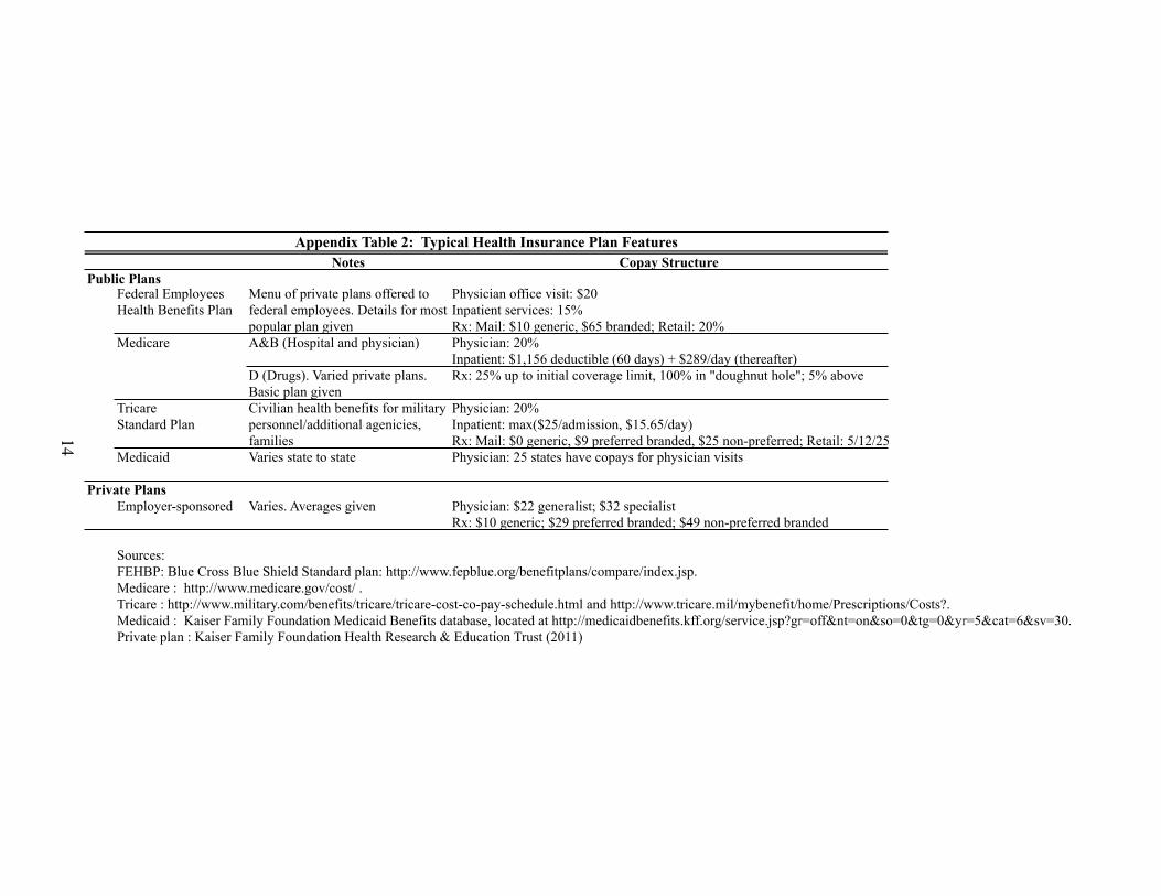
Notes Copay StructurePublic Plans

Physician office visit: $20Inpatient services: 15% Rx: Mail: $10 generic, $65 branded; Retail: 20%

Medicare A&B (Hospital and physician) Physician: 20%Inpatient: $1,156 deductible (60 days) + $289/day (thereafter)Rx: 25% up to initial coverage limit, 100% in "doughnut hole"; 5% above

Tricare Physician: 20%Standard Plan Inpatient: max($25/admission, $15.65/day)

Rx: Mail: $0 generic, $9 preferred branded, $25 non-preferred; Retail: 5/12/25Medicaid Varies state to state Physician: 25 states have copays for physician visits

Private PlansEmployer-sponsored Varies. Averages given Physician: $22 generalist; $32 specialist

Rx: $10 generic; $29 preferred branded; $49 non-preferred branded

Sources:FEHBP: Blue Cross Blue Shield Standard plan: http://www.fepblue.org/benefitplans/compare/index.jsp.Medicare : http://www.medicare.gov/cost/ .Tricare : http://www.military.com/benefits/tricare/tricare-cost-co-pay-schedule.html and http://www.tricare.mil/mybenefit/home/Prescriptions/Costs?.Medicaid : Kaiser Family Foundation Medicaid Benefits database, located at http://medicaidbenefits.kff.org/service.jsp?gr=off&nt=on&so=0&tg=0&yr=5&cat=6&sv=30.Private plan : Kaiser Family Foundation Health Research & Education Trust (2011)

Appendix Table 2: Typical Health Insurance Plan Features

Menu of private plans offered to federal employees. Details for most popular plan given

D (Drugs). Varied private plans. Basic plan givenCivilian health benefits for military personnel/additional agenicies, families

Federal Employees Health Benefits Plan

14

Appendix References

Anderson, Keaven M, Patricia M Odell, Peter WF Wilson, and William B Kannel, “Cardiovascular Disease RiskProfiles,” American Heart Journal, 1991, 121 (1), 293–298.

Baiget, C, A Keech, P.M. Kearney et al., “Efficacy and Safety of Cholesterol-Lowering Treatment: ProspectiveMeta-Analysis of Data from 90,056 Participants in 14 Randomised Trials of Statins,” Lancet, October 2005, 366(9493), 1267–1278.

Bailey, CJ and Michael Kodack, “Patient Adherence to Medication Requirements for Therapy of Type 2 Diabetes,”International Journal of Clinical Practice, 2011, 65 (3), 314–322.

Butler, Janet A, Paul Roderick, Mark Mullee, Juan C Mason, and Robert C Peveler, “Frequency and Impactof Nonadherence to Immunosuppressants After Renal Transplantation: a Systematic Review,” Transplantation,2004, 77 (5), 769–776.

CDC Vital Signs: High Blood Pressure and Cholesterol, National Center for Chronic Disease Prevention and HealthPromotion, 2011.

Chambers, Christopher P and Paul J Healy, “Updating Toward the Signal,” Economic Theory, 2012, 50 (3), 765–786.

Chandra, Amitabh, Jonathan Gruber, and Robin McKnight, “Patient Cost-Sharing and Hospitalization Offsets inthe Elderly,” The American Economic Review, 2010, 100 (1), 193.

Chernew, Michael E, Mayur R Shah, Arnold Wegh, Stephen N Rosenberg, Iver A Juster, Allison B Rosen,Michael C Sokol, Kristina Yu-Isenberg, and A Mark Fendrick, “Impact of Decreasing Copayments on Med-ication Adherence Within a Disease Management Environment,” Health Affairs, 2008, 27 (1), 103–112.

Chou, Roger, Jamie Baisden, Eugene J Carragee, Daniel K Resnick, William O Shaffer, and John D Loeser,“Surgery for Low Back Pain: A Review of the Evidence for an American Pain Society Clinical Practice Guide-line,” Spine, 2009, 34 (10), 1094–1109.

Choudhry, Niteesh K, Jerry Avorn, Robert J Glynn, Elliott M Antman, Sebastian Schneeweiss, MicheleToscano, Lonny Reisman, Joaquim Fernandes, Claire Spettell, Joy L Lee et al., “Full Coverage for Preven-tive Medications After Myocardial Infarction,” New England Journal of Medicine, 2011, 365 (22), 2088–2097.

Collins, J.W. and R.J David, “Differences in Neonatal Mortality by Race, Income, and Prenatal Care,” Ethnicity andDisease, 1992, 2 (1), 18–26.

Cutler, David M, Genia Long, Ernst R Berndt, Jimmy Royer, Andre-Anne Fournier, Alicia Sasser, and PierreCremieux, “The Value of Antihypertensive Drugs: a Perspective on Medical Innovation,” Health Affairs, 2007,26 (1), 97–110.

Dobbels, Fabienne, Todd Ruppar, Sabina De Geest, A Decorte, Van Damme-Lombaerts, RN Fine et al., “Ad-herence to the Immunosuppressive Regimen in Pediatric Kidney Transplant Recipients: A Systematic Review,”Pediatric Transplantation, 2010, 14 (5), 603–613.

Froom, Jack, Larry Culpepper, Paul Grob, Aad Bartelds, Peter Bowers, Charles Bridges-Webb, Inese Grava-Gubins, Larry Green, Jacqueline Lion, Bertino Somaini et al., “Diagnosis and Antibiotic Treatment of AcuteOtitis Media: Report from International Primary Care Network.,” BMJ: British Medical Journal, 1990, 300(6724), 582.

Gortmaker, Steven Lawrance, “The Effects of Prenatal Care Upon the Health of the Newborn,” American Journalof Public Health, 1979, 69 (7), 653–660.

Hodgson, Thomas A and Liming Cai, “Medical Care Expenditures for Hypertension, its Complications, and itsComorbidities,” Medical Care, 2001, 39 (6), 599–615.

Holmberg, Lars, Anna Bill-Axelson, Fred Helgesen, Jaakko O Salo, Per Folmerz, Michael Haggman, Swen-Olof Andersson, Anders Spaangberg, Christer Busch, Steg Nordling et al., “A Randomized Trial ComparingRadical Prostatectomy with Watchful Waiting in Early Prostate Cancer,” New England Journal of Medicine,2002, 347 (11), 781–789.

Hsu, John, Mary Price, Jie Huang, Richard Brand, Vicki Fung, Rita Hui, Bruce Fireman, Joseph P Newhouse,and Joseph V Selby, “Unintended Consequences of Caps on Medicare Drug Benefits,” New England Journal ofMedicine, 2006, 354 (22), 2349–2359.

Jarvik, Jeffrey G, William Hollingworth, Brook Martin, Scott S Emerson, Darryl T Gray, Steven Overman,David Robinson, Thomas Staiger, Frank Wessbecher, Sean D Sullivan et al., “Rapid Magnetic ResonanceImaging vs Radiographs for Patients with Low Back Pain: A Randomized Controlled Trial,” Jama, 2003, 289(21), 2810–2818.

Kramer, Judith M, Bradley Hammill, Kevin J Anstrom, Donald Fetterolf, Richard Snyder, John P Charde,Barbara S Hoffman, Nancy Allen LaPointe, and Eric Peterson, “National Evaluation of Adherence to Beta-Blocker Therapy for 1 Year After Acute Myocardial Infarction in Patients with Commercial Health Insurance,”American Heart Journal, 2006, 152 (3), 454–e1.

Krishnan, Jerry A, Kristin A Riekert, Jonathan V McCoy, Dana Y Stewart, Spencer Schmidt, Arjun Chan-mugam, Peter Hill, and Cynthia S Rand, “Corticosteroid Use after Hospital Discharge Among High-RiskAdults with Asthma,” American Journal of Respiratory and Critical Care Medicine, 2004, 170 (12), 1281–1285.

, Steven Q Davis, Edward T Naureckas, Peter Gibson, and Brian H Rowe, “An Umbrella Review: Corticos-teroid Therapy for Adults with Acute Asthma,” The American Journal of Medicine, 2009, 122 (11), 977–991.

Landsman, Pamela B, Winnie Yu, XiaoFeng Liu, Steven M Teutsch, and Mark L Berger, “Impact of 3-TierPharmacy Benefit Design and Increased Consumer Cost-Sharing on Drug Utilization,” The American Journal ofManaged Care, 2005, 11 (10), 621–628.

Lohr, Kathleen N, Robert H Brook, Caren J Kamberg, George A Goldberg, Arleen Leibowitz, Joan Keesey,David Reboussin, and Joseph P Newhouse, “Use of Medical Care in the RAND Health Insurance Experiment:Diagnosis and Service-Specific Analyses in a Randomized Controlled Trial,” Medical Care, 1986, pp. S1–S87.

Long, Genia, David Cutler, Ernst R Berndt, Jimmy Royer, Andre-Anne Fournier, Alicia Sasser, and PierreCremieux, “The Impact of Antihypertensive Drugs On the Number and Risk of Death, Stroke and MyocardialInfarction in the United States,” Technical Report, National Bureau of Economic Research 2006.

Lu-Yao, GL and ER Greenberg, “Changes in Prostate Cancer Incidence and Treatment in USA,” The Lancet, 1994,343 (8892), 251–254.

McInerny, Thomas K, William L Cull, and Beth K Yudkowsky, “Physician Reimbursement Levels and Adherenceto American Academy of Pediatrics Well-Visit and Immunization Recommendations,” Pediatrics, 2005, 115 (4),833–838.

McKenney, James M, Wendy P Munroe, and Jackson T Wright, “Impact of an Electronic Medication ComplianceAid on Long-Term Blood Pressure Control,” The Journal of Clinical Pharmacology, 1992, 32 (3), 277–283.

Pittman, Donald G, William Chen, Steven J Bowlin, and JoAnne M Foody, “Adherence to Statins, SubsequentHealthcare Costs, and Cardiovascular Hospitalizations,” The American Journal of Cardiology, 2011, 107 (11),1662–1666.

Ross, Louie E, Zahava Berkowitz, and Donatus U Ekwueme, “Use of the Prostate-Specific Antigen Test AmongUS Men: Findings from the 2005 National Health Interview Survey,” Cancer Epidemiology Biomarkers andPrevention, 2008, 17 (3), 636–644.

Sanders, Sharon, Paul P Glasziou, C Del Mar, and M Rovers, “Antibiotics for Acute Otitis Media in Children,”Cochrane Database of Systematic Reviews, 2004, 1.

Schroder, Fritz H, Jonas Hugosson, Monique J Roobol, Teuvo LJ Tammela, Stefano Ciatto, Vera Nelen, MaciejKwiatkowski, Marcos Lujan, Hans Lilja, Marco Zappa et al., “Prostate-Cancer Mortality at 11 Years ofFollow-Up,” New England Journal of Medicine, 2012, 366 (11), 981–990.

Schroeder, Knut, T Fahey, and S Ebrahim, “Interventions for Improving Adherence to Treatment in Patients withHigh Blood Pressure in Ambulatory Settings,” Cochrane Library, 2008, (4).

Selvin, Elizabeth, Shari Bolen, Hsin-Chieh Yeh, Crystal Wiley, Lisa M Wilson, Spyridon S Marinopoulos,Leonard Feldman, Jason Vassy, Renee Wilson, Eric B Bass et al., “Cardiovascular Outcomes in Trials of OralDiabetes Medications: a Systematic Review,” Archives of Internal Medicine, 2008, 168 (19), 2070–2080.

Sloan, Frank A, M Angelyn Bethel, Paul P Lee, Derek S Brown, and Mark N Feinglos, “Adherence to Guidelinesand Its Effects on Hospitalizations with Complications of Type 2 Diabetes,” The Review of Diabetic Studies,2004, 1 (1), 29.

Soumerai, Stephen B, Thomas J McLaughlin, Donna Spiegelman, Ellen Hertzmark, George Thibault, andLee Goldman, “Adverse outcomes of underuse of Beta-Blockers in Elderly Survivors of Acute MyocardialInfarction,” Journal of the American Medical Association, 1997, 277 (2), 115–121.

Wang, Guijing, “Cost-Effectiveness of Hypertension Control,” iHEA Abstract, 2011.

Yusuf, Salim, Richard Peto, John Lewis, Rory Collins, and Peter Sleight, “Beta Blockade During and AfterMyocardial Infarction: an Overview of the Randomized Trials,” Progress in Cardiovascular Diseases, 1985, 27(5), 335–371.