Beirut Master 4000 Progress Report ECSE-4460 Control System Design

Team 2 Larry Cole Vinay Shah Danish Zia

Bert Hallonquist

Wednesday, March 30, 2005

Rensselaer Polytechnic Institute

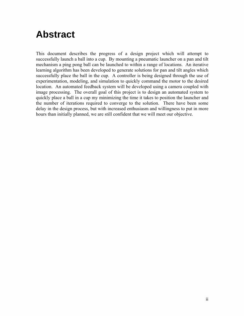
Abstract This document describes the progress of a design project which will attempt to successfully launch a ball into a cup. By mounting a pneumatic launcher on a pan and tilt mechanism a ping pong ball can be launched to within a range of locations. An iterative learning algorithm has been developed to generate solutions for pan and tilt angles which successfully place the ball in the cup. A controller is being designed through the use of experimentation, modeling, and simulation to quickly command the motor to the desired location. An automated feedback system will be developed using a camera coupled with image processing. The overall goal of this project is to design an automated system to quickly place a ball in a cup my minimizing the time it takes to position the launcher and the number of iterations required to converge to the solution. There have been some delay in the design process, but with increased enthusiasm and willingness to put in more hours than initially planned, we are still confident that we will meet our objective.

ii

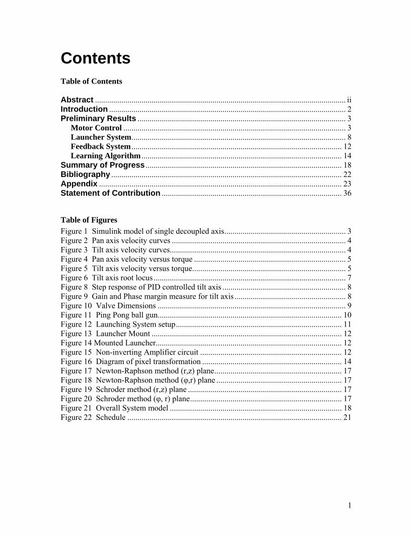
Contents Table of Contents Abstract ............................................................................................................................ iiIntroduction ..................................................................................................................... 2 Preliminary Results ....................................................................................................... 3 Motor Control .............................................................................................................. 3 Launcher System.......................................................................................................... 8 Feedback System ........................................................................................................ 12 Learning Algorithm ................................................................................................... 14 Summary of Progress ................................................................................................. 18 Bibliography .................................................................................................................. 22 Appendix ........................................................................................................................ 23 Statement of Contribution ......................................................................................... 36

Table of Figures Figure 1 Simulink model of single decoupled axis............................................................ 3 Figure 2 Pan axis velocity curves ...................................................................................... 4 Figure 3 Tilt axis velocity curves....................................................................................... 4 Figure 4 Pan axis velocity versus torque ........................................................................... 5 Figure 5 Tilt axis velocity versus torque............................................................................ 5 Figure 6 Tilt axis root locus ............................................................................................... 7 Figure 8 Step response of PID controlled tilt axis ............................................................. 8 Figure 9 Gain and Phase margin measure for tilt axis ....................................................... 8 Figure 10 Valve Dimensions ............................................................................................. 9 Figure 11 Ping Pong ball gun........................................................................................... 10 Figure 12 Launching System setup.................................................................................. 11 Figure 13 Launcher Mount .............................................................................................. 12 Figure 14 Mounted Launcher............................................................................................ 12 Figure 15 Non-inverting Amplifier circuit ...................................................................... 12 Figure 16 Diagram of pixel transformation ..................................................................... 14 Figure 17 Newton-Raphson method (r,z) plane............................................................... 17 Figure 18 Newton-Raphson method (φ,r) plane .............................................................. 17 Figure 19 Schroder method (r,z) plane ............................................................................ 17 Figure 20 Schroder method (φ, r) plane........................................................................... 17 Figure 21 Overall System model ..................................................................................... 18 Figure 22 Schedule .......................................................................................................... 21

1

Introduction

For this project we will launch a projectile toward a target. We will mount a launcher on the pan-and-tilt device, so that the launch angle is determined by the pan-and-tilt. After the ball is fired a camera will capture the point where the ball hits the ground. The time at which the ball strikes the ground will be determined by piezo devices placed around the area of the target. The camera will capture a single frame image of the ball and the target at this time. The image will be processed and sent to the learning algorithm which will determine the angles for the next shot. This iterative learning system will be able to hit the target within eight attempts. Our motivation was to create a machine that can automatically master the game of Beirut, a popular game among college students where players must throw ping pong balls into cups. However, the concept of the iterative learning algorithm has several applications outside of the scope of our project. This implementation can be used for military applications. Using satellite imaging, the algorithm can be used to iteratively learn how to hit targets with missiles. The robotics industry is interested in using iterative learning algorithms to develop smarter robots for various applications. The motors will be controlled by a PID controller to move the launcher into a desired position. The controllers will minimize the settling time of the response, have zero steady state error, minimum over shoot, and should be able to track a desired trajectory. Currently we have fallen behind in our planned progress, however adequate progress has been made. The launching system is connected to the air tank and is ready to be tested. It is not yet mounted on the pan-and-tilt, but the method for doing so is planned out and will be implemented soon. Modification of the launcher nozzle is a future task to be looked at. For the controller, a MATLAB script has been written and tested to identify model parameters. An initial design approach for the controllers have been established and tested with an estimated model. For the feedback system, integration of the piezo devices and camera has yet to be completed, however a MATLAB script to detect the ball and target has been completed. The learning algorithm is completed and will only require minor tweaks when implemented on the actual system. It uses the Schröder method because it converged to the solution faster than the other possible methods. Future tasks include calibrating the learning algorithm to be compatible with the feedback system and launching system. Friction identification turned out to be an unanticipated challenge in that it was more time consuming than initially planned. Another challenge was to rethink the launcher system so that pressure doesn’t build up indefinitely in the tubes. This would cause tubing to fly off of the barbs that they were attached to. In our original plans we hadn’t for-seen that this would occur.

Preliminary Results

2

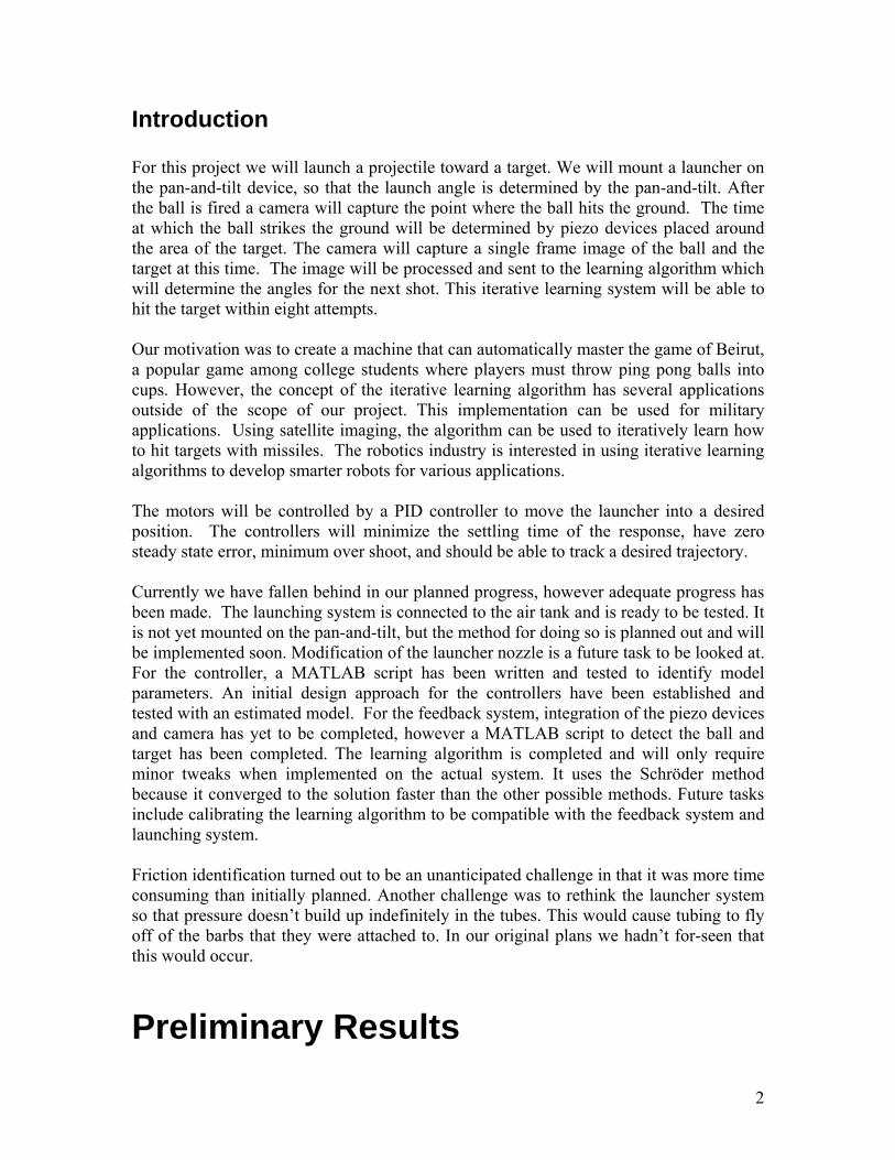
Motor Control The plant is being modeled as a system with two decoupled axis. Coupling between the two axis may occur due to Coriolis affects, however at this point we assume it to be a negligible affect and model it as noise to the system. If this assumption is proven to be invalid during model validation stages, Coriolis affects will be investigated and implemented in the model. The model of a single axis is shown in Figure 1.

Bveff

sin

voltage

data

Sign

1s

1s

Integrator

Bceff

m*g*l1/Jeff

N*Kt*Kiinput

FromWorkspace

position

v iscous f riction

Coulomb f riction

grav ityloading

Figure 1 Simulink model of single decoupled axis The system transforms an input voltage to a position of the axis (in radians) while considering affects due to friction and gravity loading. Non-linearities such as Coulomb friction, quantization, and saturation exist when attempting to realistically model the system. By ignoring quantization and saturation affects, a differential equation of the system can be written as:

sin ( )eff m v cJ N mgl B B Signθ τ θ θ= + − − θ (1) Where Jeff is the effective load inertia, N is the gear ratio, mτ is the motor torque, m is the mass, g is gravity, l is the center of gravity of the load, vB is the viscous friction, and cB is the Coulomb fiction. The motor torque can be calculated as follow: m VNK Kt iτ = (2) Where V is the input voltage, N is the gear ratio once again, Kt is the torque constant (.0436 N*m/A in our case) and Ki is the amplifier gain (0.1 Amp/volt). Thus the parameters which need to be identified are the viscous and Coulomb friction, the effective inertia, and the gravity loading term mgl. Multiple methods of obtaining this data are being explored in order to find the most accurate representation of the system. [5]

3

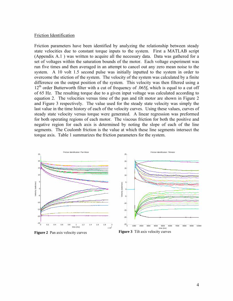
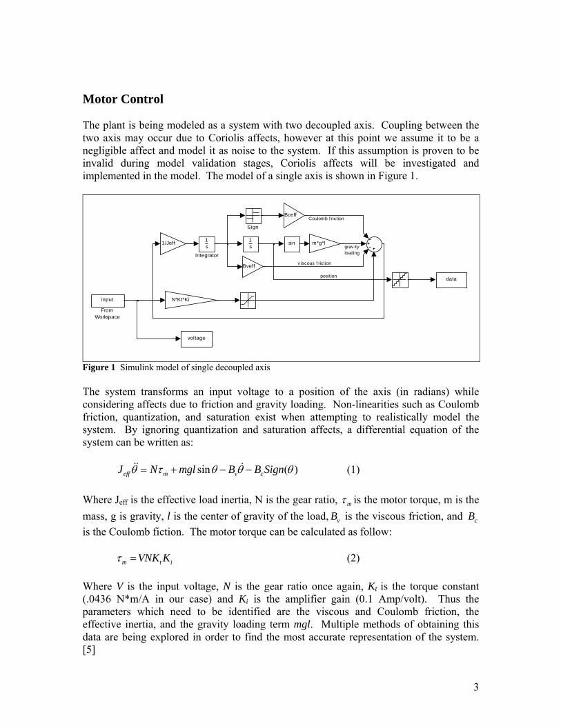
Friction Identification Friction parameters have been identified by analyzing the relationship between steady state velocities due to constant torque inputs to the system. First a MATLAB script (Appendix A.1 ) was written to acquire all the necessary data. Data was gathered for a set of voltages within the saturation bounds of the motor. Each voltage experiment was run five times and then averaged in an attempt to cancel out any zero mean noise to the system. A 10 volt 1.5 second pulse was initially inputted to the system in order to overcome the stiction of the system. The velocity of the system was calculated by a finite difference on the output position of the system. This velocity was then filtered using a 12th order Butterworth filter with a cut of frequency of .065fs which is equal to a cut off of 65 Hz. The resulting torque due to a given input voltage was calculated according to equation 2. The velocities versus time of the pan and tilt motor are shown in Figure 2 and Figure 3 respectively. The value used for the steady state velocity was simply the last value in the time history of each of the velocity curves. Using these values, curves of steady state velocity versus torque were generated. A linear regression was preformed for both operating regions of each motor. The viscous friction for both the positive and negative region for each axis is determined by noting the slope of each of the line segments. The Coulomb friction is the value at which these line segments intersect the torque axis. Table 1 summarizes the friction parameters for the system.

0 0.2 0.4 0.6 0.8 1 1.2 1.4 1.6 1.8 2

x 104

-25

-20

-15

-10

-5

0

5

10

15

20

25

Vel

ocity

(rad

s/se

c)

time (ms)

Friction Identification: Pan Motor

Figure 2 Pan axis velocity curves

0 1000 2000 3000 4000 5000 6000 7000 8000 9000 10000-25

-20

-15

-10

-5

0

5

10

15

20

25

Vel

ocity

(rad

s/se

c)

time (ms)

Friction Identification: Tiltmotor

Figure 3 Tilt axis velocity curves

4

-20 -15 -10 -5 0 5 10 15 20-0.1

-0.08

-0.06

-0.04

-0.02

0

0.02

0.04

0.06

0.08

0.1

velocity (rads/sec)

torq

ue (N

*m)

Friction Indentification: Pan Motor

Figure 4 Pan axis velocity versus torque

-25 -20 -15 -10 -5 0 5 10 15 20 25-0.2

-0.15

-0.1

-0.05

0

0.05

0.1

0.15

velocity (rads/sec)

torq

ue (N

*m)

Friction Indentification: Tilt Motor

Figure 5 Tilt axis velocity versus torque

Pan Motor Positive Negative Viscous (N.m.s/rad) 0.00066913 0.00069303

Coulomb (N.m) 0.080058 -0.071475

Tilt Motor Positive Negative Viscous (N.m.s/rad) 0.0015316 0.0016016

Coulomb (N.m) 0.075495 -0.077283

Table 1 Summary of friction parameters Inertia Estimates and Gravity Loading Two of the required parameters to create the system model are the load inertia (JL) as well as the gravity loading. Due to the complexity of the model, both these parameters were calculated using the SolidWorks 2004 software. First, the launcher and mount for our system was created inside SolidWorks 2004, and attached to the existed pan-tilt mechanism model designed by Ben Potsaid. Next, the density of each part of the model was assigned. Then a coordinate system relative to each of the two motors was defined, and aligned with the rotation axis. All the parts causing an inertial load on the each motor were selected and their “Mass Properties” relative to the coordinate system defined for that motor was displayed. This revealed the 3x3 inertia matrix, as well as the total mass and center of mass of these parts. From these, the load inertia and gravity loading were calculated. Parameter Identification Another method uses a least squares estimation method to determine all the parameters in a single experiment. However, the results of this method are dependant on the type of input given. The input must “sufficiently exciting” which means the effects of the different parameters can be observed. Thus, a good input for one system may be a poor input for another. By lumping the parameters in equation 2 the dynamic model of a single axis can rewritten as:

5

1 2 3 4( ) sina a Sign a V aθ θ θ= − − + + θ

ff

ff

ff

eff

(3) By comparing equation 3 with equation 2 it is easy to observe that

1 v e = B /Ja (4)

2 c e = B /Ja (5)

3 t i e = K K N/Ja (6)

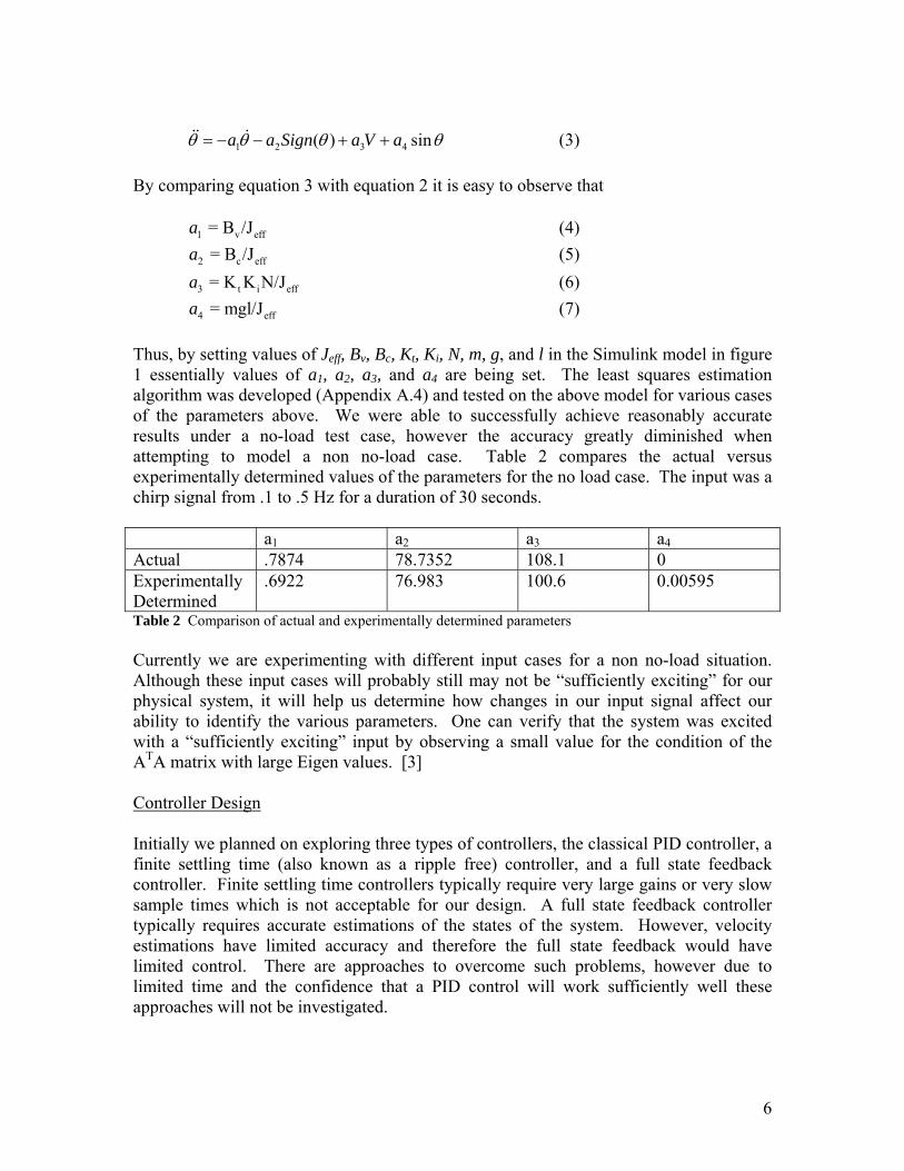
4 = mgl/Ja (7) Thus, by setting values of Jeff, Bv, Bc, Kt, Ki, N, m, g, and l in the Simulink model in figure 1 essentially values of a1, a2, a3, and a4 are being set. The least squares estimation algorithm was developed (Appendix A.4) and tested on the above model for various cases of the parameters above. We were able to successfully achieve reasonably accurate results under a no-load test case, however the accuracy greatly diminished when attempting to model a non no-load case. Table 2 compares the actual versus experimentally determined values of the parameters for the no load case. The input was a chirp signal from .1 to .5 Hz for a duration of 30 seconds. a1 a2 a3 a4Actual .7874 78.7352 108.1 0 Experimentally Determined

.6922 76.983 100.6 0.00595

Table 2 Comparison of actual and experimentally determined parameters Currently we are experimenting with different input cases for a non no-load situation. Although these input cases will probably still may not be “sufficiently exciting” for our physical system, it will help us determine how changes in our input signal affect our ability to identify the various parameters. One can verify that the system was excited with a “sufficiently exciting” input by observing a small value for the condition of the ATA matrix with large Eigen values. [3] Controller Design Initially we planned on exploring three types of controllers, the classical PID controller, a finite settling time (also known as a ripple free) controller, and a full state feedback controller. Finite settling time controllers typically require very large gains or very slow sample times which is not acceptable for our design. A full state feedback controller typically requires accurate estimations of the states of the system. However, velocity estimations have limited accuracy and therefore the full state feedback would have limited control. There are approaches to overcome such problems, however due to limited time and the confidence that a PID control will work sufficiently well these approaches will not be investigated.

6

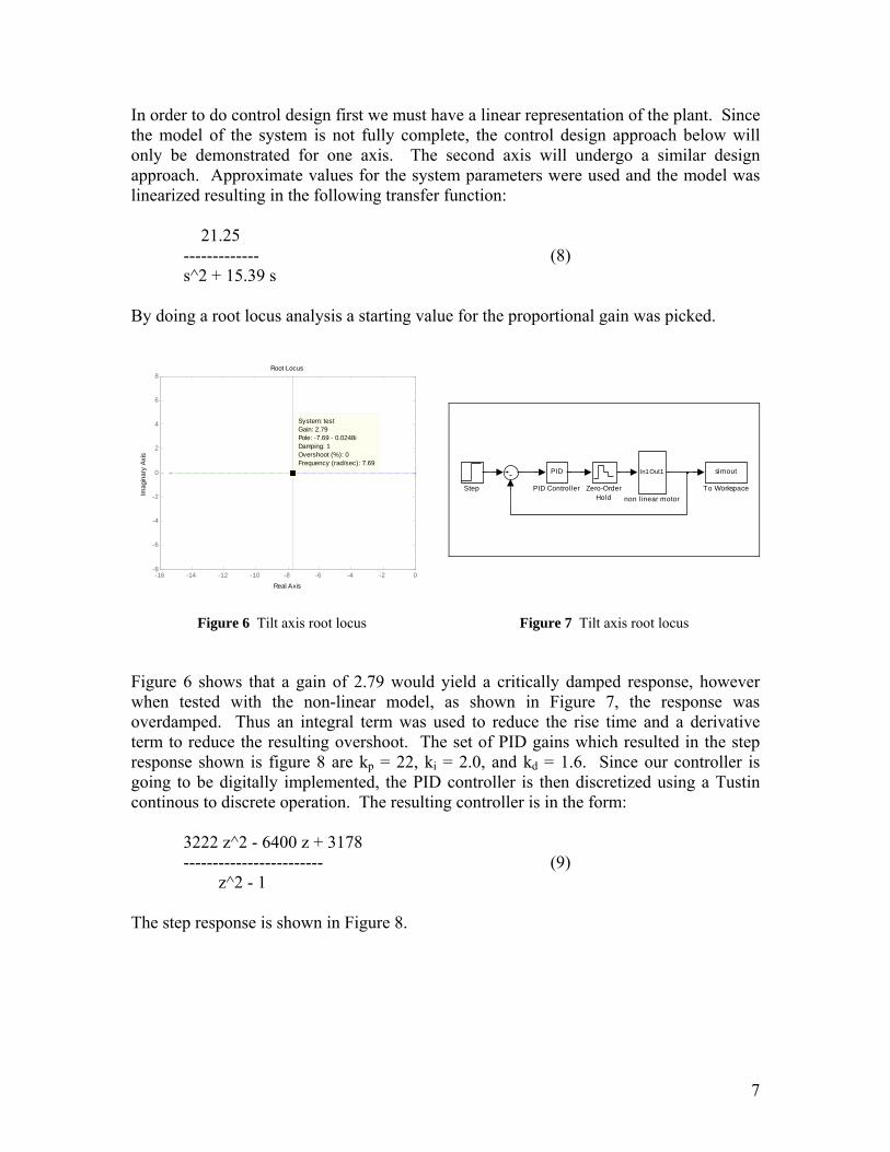
In order to do control design first we must have a linear representation of the plant. Since the model of the system is not fully complete, the control design approach below will only be demonstrated for one axis. The second axis will undergo a similar design approach. Approximate values for the system parameters were used and the model was linearized resulting in the following transfer function:

21.25 ------------- (8) s^2 + 15.39 s

By doing a root locus analysis a starting value for the proportional gain was picked.

-16 -14 -12 -10 -8 -6 -4 -2 0-8

-6

-4

-2

0

2

4

6

8

System: testGain: 2.79Pole: -7.69 - 0.0248iDamping: 1Overshoot (%): 0Frequency (rad/sec): 7.69

Root Locus

Real Axis

Imag

inar

y Ax

is

In1Out1

non linear motorZero-Order

Hold

simout

To WorkspaceStep

PID

PID Controller

Figure 6 Tilt axis root locus Figure 7 Tilt axis root locus

Figure 6 shows that a gain of 2.79 would yield a critically damped response, however when tested with the non-linear model, as shown in Figure 7, the response was overdamped. Thus an integral term was used to reduce the rise time and a derivative term to reduce the resulting overshoot. The set of PID gains which resulted in the step response shown is figure 8 are kp = 22, ki = 2.0, and kd = 1.6. Since our controller is going to be digitally implemented, the PID controller is then discretized using a Tustin continous to discrete operation. The resulting controller is in the form:

3222 z^2 - 6400 z + 3178 ------------------------ (9) z^2 - 1

The step response is shown in Figure 8.

7

0 1 2 3 4 5 6 7 8 9 100

0.2

0.4

0.6

0.8

1

1.2

1.4

time (s)

posi

tion

(rad)

tilt axis step response

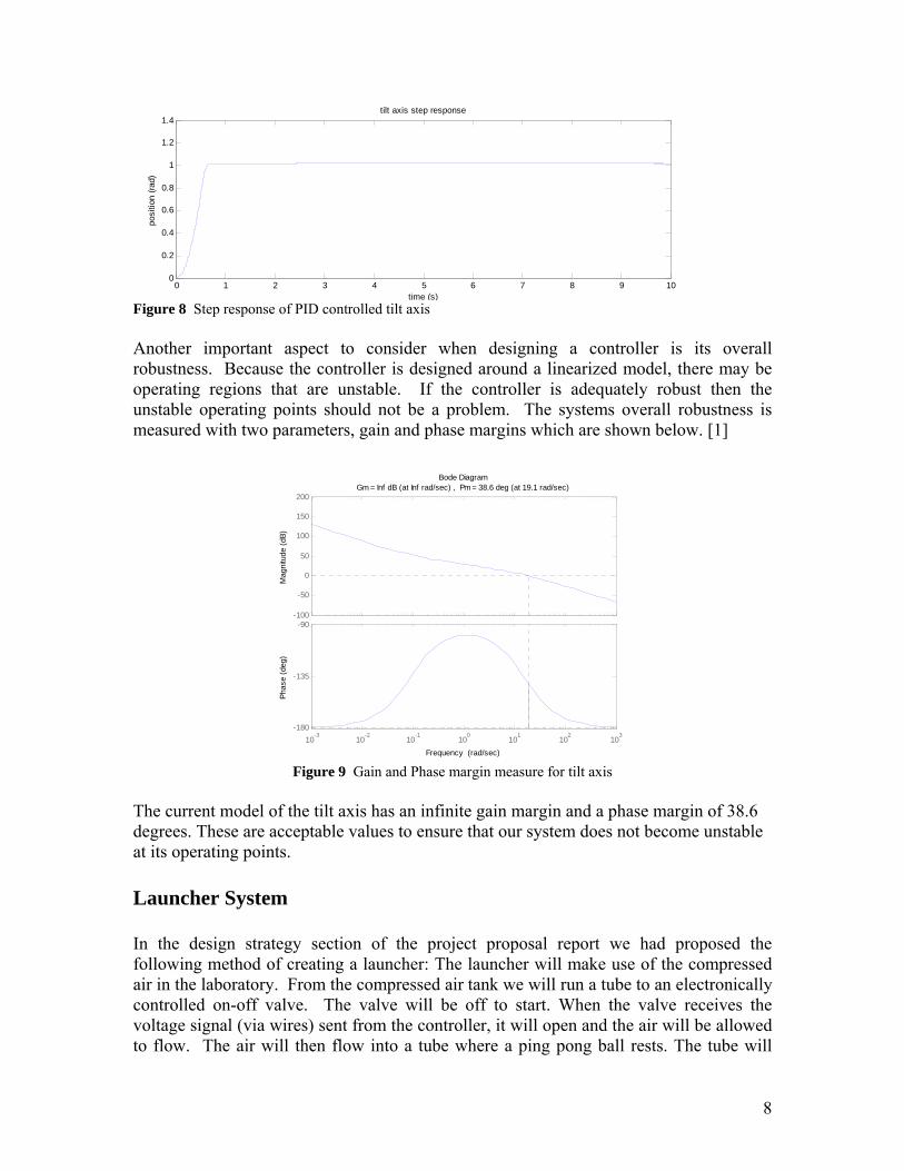
Figure 8 Step response of PID controlled tilt axis Another important aspect to consider when designing a controller is its overall robustness. Because the controller is designed around a linearized model, there may be operating regions that are unstable. If the controller is adequately robust then the unstable operating points should not be a problem. The systems overall robustness is measured with two parameters, gain and phase margins which are shown below. [1]

-100

-50

0

50

100

150

200

Mag

nitu

de (d

B)

10-3

10-2

10-1

100

101

102

103

-180

-135

-90

Phas

e (d

eg)

Bode DiagramGm = Inf dB (at Inf rad/sec) , Pm = 38.6 deg (at 19.1 rad/sec)

Frequency (rad/sec) Figure 9 Gain and Phase margin measure for tilt axis

The current model of the tilt axis has an infinite gain margin and a phase margin of 38.6 degrees. These are acceptable values to ensure that our system does not become unstable at its operating points. Launcher System In the design strategy section of the project proposal report we had proposed the following method of creating a launcher: The launcher will make use of the compressed air in the laboratory. From the compressed air tank we will run a tube to an electronically controlled on-off valve. The valve will be off to start. When the valve receives the voltage signal (via wires) sent from the controller, it will open and the air will be allowed to flow. The air will then flow into a tube where a ping pong ball rests. The tube will

8

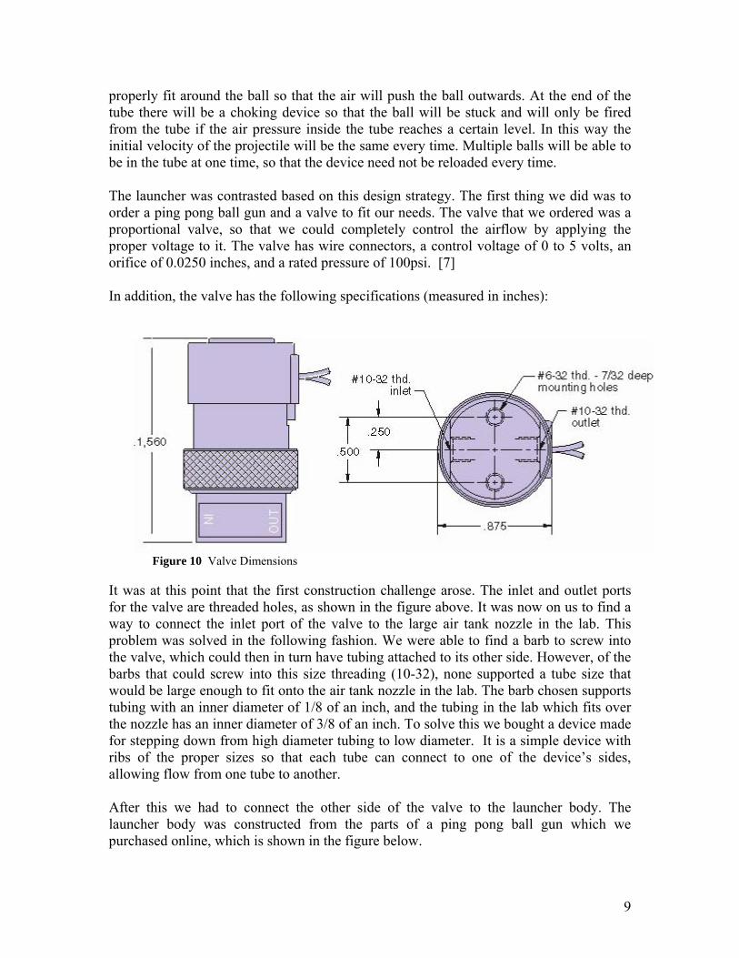
properly fit around the ball so that the air will push the ball outwards. At the end of the tube there will be a choking device so that the ball will be stuck and will only be fired from the tube if the air pressure inside the tube reaches a certain level. In this way the initial velocity of the projectile will be the same every time. Multiple balls will be able to be in the tube at one time, so that the device need not be reloaded every time. The launcher was contrasted based on this design strategy. The first thing we did was to order a ping pong ball gun and a valve to fit our needs. The valve that we ordered was a proportional valve, so that we could completely control the airflow by applying the proper voltage to it. The valve has wire connectors, a control voltage of 0 to 5 volts, an orifice of 0.0250 inches, and a rated pressure of 100psi. [7] In addition, the valve has the following specifications (measured in inches):

Figure 10 Valve Dimensions

It was at this point that the first construction challenge arose. The inlet and outlet ports for the valve are threaded holes, as shown in the figure above. It was now on us to find a way to connect the inlet port of the valve to the large air tank nozzle in the lab. This problem was solved in the following fashion. We were able to find a barb to screw into the valve, which could then in turn have tubing attached to its other side. However, of the barbs that could screw into this size threading (10-32), none supported a tube size that would be large enough to fit onto the air tank nozzle in the lab. The barb chosen supports tubing with an inner diameter of 1/8 of an inch, and the tubing in the lab which fits over the nozzle has an inner diameter of 3/8 of an inch. To solve this we bought a device made for stepping down from high diameter tubing to low diameter. It is a simple device with ribs of the proper sizes so that each tube can connect to one of the device’s sides, allowing flow from one tube to another. After this we had to connect the other side of the valve to the launcher body. The launcher body was constructed from the parts of a ping pong ball gun which we purchased online, which is shown in the figure below.

9

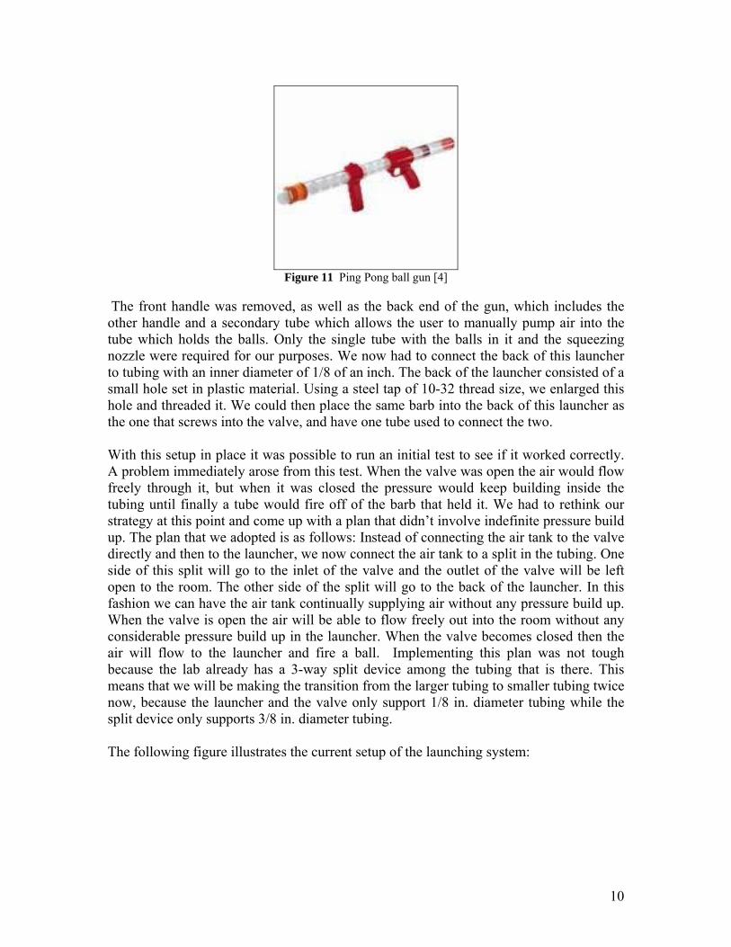
Figure 11 Ping Pong ball gun [4]

The front handle was removed, as well as the back end of the gun, which includes the other handle and a secondary tube which allows the user to manually pump air into the tube which holds the balls. Only the single tube with the balls in it and the squeezing nozzle were required for our purposes. We now had to connect the back of this launcher to tubing with an inner diameter of 1/8 of an inch. The back of the launcher consisted of a small hole set in plastic material. Using a steel tap of 10-32 thread size, we enlarged this hole and threaded it. We could then place the same barb into the back of this launcher as the one that screws into the valve, and have one tube used to connect the two. With this setup in place it was possible to run an initial test to see if it worked correctly. A problem immediately arose from this test. When the valve was open the air would flow freely through it, but when it was closed the pressure would keep building inside the tubing until finally a tube would fire off of the barb that held it. We had to rethink our strategy at this point and come up with a plan that didn’t involve indefinite pressure build up. The plan that we adopted is as follows: Instead of connecting the air tank to the valve directly and then to the launcher, we now connect the air tank to a split in the tubing. One side of this split will go to the inlet of the valve and the outlet of the valve will be left open to the room. The other side of the split will go to the back of the launcher. In this fashion we can have the air tank continually supplying air without any pressure build up. When the valve is open the air will be able to flow freely out into the room without any considerable pressure build up in the launcher. When the valve becomes closed then the air will flow to the launcher and fire a ball. Implementing this plan was not tough because the lab already has a 3-way split device among the tubing that is there. This means that we will be making the transition from the larger tubing to smaller tubing twice now, because the launcher and the valve only support 1/8 in. diameter tubing while the split device only supports 3/8 in. diameter tubing. The following figure illustrates the current setup of the launching system:

10

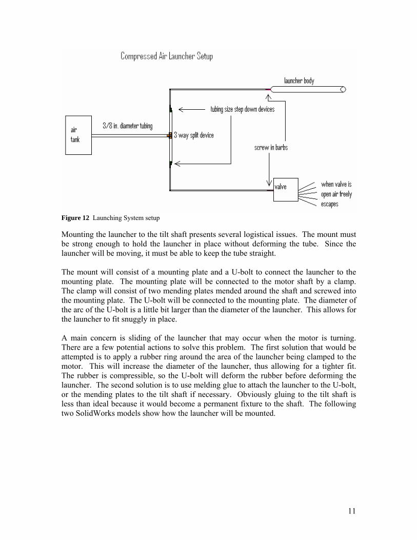
Figure 12 Launching System setup Mounting the launcher to the tilt shaft presents several logistical issues. The mount must be strong enough to hold the launcher in place without deforming the tube. Since the launcher will be moving, it must be able to keep the tube straight. The mount will consist of a mounting plate and a U-bolt to connect the launcher to the mounting plate. The mounting plate will be connected to the motor shaft by a clamp. The clamp will consist of two mending plates mended around the shaft and screwed into the mounting plate. The U-bolt will be connected to the mounting plate. The diameter of the arc of the U-bolt is a little bit larger than the diameter of the launcher. This allows for the launcher to fit snuggly in place. A main concern is sliding of the launcher that may occur when the motor is turning. There are a few potential actions to solve this problem. The first solution that would be attempted is to apply a rubber ring around the area of the launcher being clamped to the motor. This will increase the diameter of the launcher, thus allowing for a tighter fit. The rubber is compressible, so the U-bolt will deform the rubber before deforming the launcher. The second solution is to use melding glue to attach the launcher to the U-bolt, or the mending plates to the tilt shaft if necessary. Obviously gluing to the tilt shaft is less than ideal because it would become a permanent fixture to the shaft. The following two SolidWorks models show how the launcher will be mounted.

11

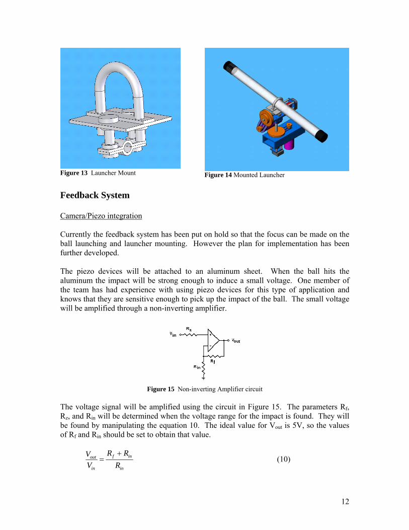
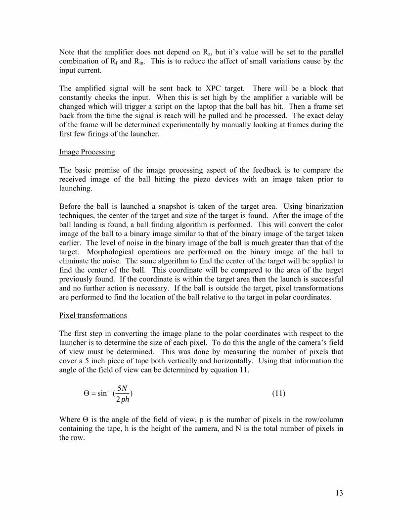
Figure 13 Launcher Mount

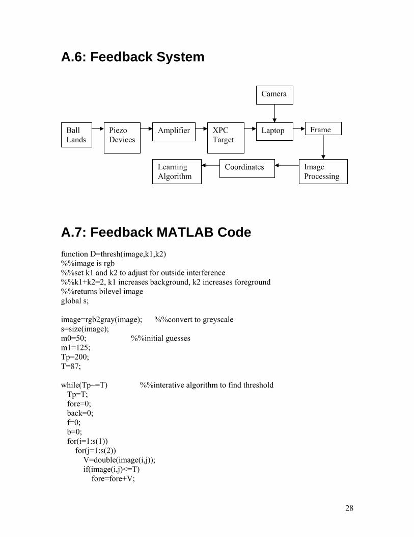
Figure 14 Mounted Launcher Feedback System Camera/Piezo integration Currently the feedback system has been put on hold so that the focus can be made on the ball launching and launcher mounting. However the plan for implementation has been further developed. The piezo devices will be attached to an aluminum sheet. When the ball hits the aluminum the impact will be strong enough to induce a small voltage. One member of the team has had experience with using piezo devices for this type of application and knows that they are sensitive enough to pick up the impact of the ball. The small voltage will be amplified through a non-inverting amplifier.

Figure 15 Non-inverting Amplifier circuit

The voltage signal will be amplified using the circuit in Figure 15. The parameters Rf, Rz, and Rin will be determined when the voltage range for the impact is found. They will be found by manipulating the equation 10. The ideal value for Vout is 5V, so the values of Rf and Rin should be set to obtain that value.

in

inf

in

out

RRR

VV +

= (10)

12

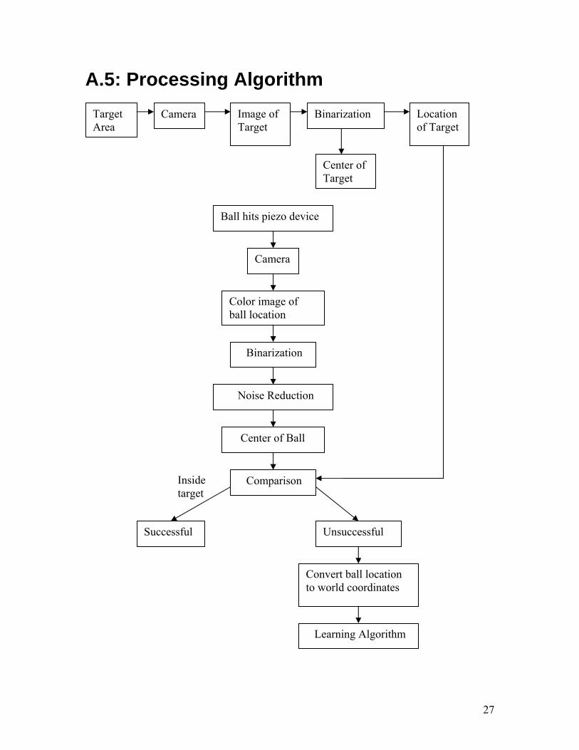
Note that the amplifier does not depend on Rz, but it’s value will be set to the parallel combination of Rf and Rin. This is to reduce the affect of small variations cause by the input current. The amplified signal will be sent back to XPC target. There will be a block that constantly checks the input. When this is set high by the amplifier a variable will be changed which will trigger a script on the laptop that the ball has hit. Then a frame set back from the time the signal is reach will be pulled and be processed. The exact delay of the frame will be determined experimentally by manually looking at frames during the first few firings of the launcher. Image Processing The basic premise of the image processing aspect of the feedback is to compare the received image of the ball hitting the piezo devices with an image taken prior to launching. Before the ball is launched a snapshot is taken of the target area. Using binarization techniques, the center of the target and size of the target is found. After the image of the ball landing is found, a ball finding algorithm is performed. This will convert the color image of the ball to a binary image similar to that of the binary image of the target taken earlier. The level of noise in the binary image of the ball is much greater than that of the target. Morphological operations are performed on the binary image of the ball to eliminate the noise. The same algorithm to find the center of the target will be applied to find the center of the ball. This coordinate will be compared to the area of the target previously found. If the coordinate is within the target area then the launch is successful and no further action is necessary. If the ball is outside the target, pixel transformations are performed to find the location of the ball relative to the target in polar coordinates. Pixel transformations The first step in converting the image plane to the polar coordinates with respect to the launcher is to determine the size of each pixel. To do this the angle of the camera’s field of view must be determined. This was done by measuring the number of pixels that cover a 5 inch piece of tape both vertically and horizontally. Using that information the angle of the field of view can be determined by equation 11.

)25(sin 1

phN−=Θ (11)

Where Θ is the angle of the field of view, p is the number of pixels in the row/column containing the tape, h is the height of the camera, and N is the total number of pixels in the row.

13

The two angles found are 0.321776 of the horizontal angle, and 0.26147 for the vertical angle. Using these values the distance of pixel in the image plane can be found by equation 12.

Nhp

pD yx.sin2)(

Θ= (12)

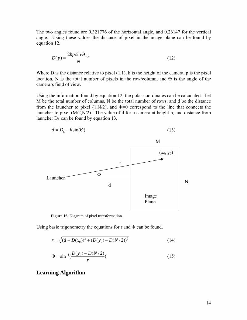
Where D is the distance relative to pixel (1,1), h is the height of the camera, p is the pixel location, N is the total number of pixels in the row/column, and Θ is the angle of the camera’s field of view. Using the information found by equation 12, the polar coordinates can be calculated. Let M be the total number of columns, N be the total number of rows, and d be the distance from the launcher to pixel (1,N/2), and Φ=0 correspond to the line that connects the launcher to pixel (M/2,N/2). The value of d for a camera at height h, and distance from launcher DL can be found by equation 13.

)sin(Θ−= hDd L (13)

M

(x0, y0)

r

Φ Launcher

N d

Image Plane

Figure 16 Diagram of pixel transformation

Using basic trigonometry the equations for r and Φ can be found.

20

20 ))2/()(())(( NDyDxDdr −++= (14)

))2/()((sin 01

rNDyD −

=Φ − (15)

Learning Algorithm

14

The learning algorithm will use an iterative control algorithm to obtain a new pan and tilt theta input based on the position error and the previous input. Initially the learning algorithm was developed using the Newton-Raphson root-finding method. Since the coordinate system being used is cylindrical, the radial distance (r) from the launcher is only affected by the tilt angle (Θ1). Similarly, the horizontal angle (φ) between the launcher-ball and launcher-center zero lines is only affected by the pan angle (Θ2). Using the general Newton-Raphson formulas, equations 16 and 17 are formed in order to determine new angles based on the previous try. The Newton-Raphson method derives a new estimate for Θ based on the previous estimate and the ratio of the error to the derivative evaluated at the previous estimate.

( )1( 1) 1( )

1( )

desired kk k

k

r rdr

d

+

−Θ = Θ +

Θ

(16)

( )2( 1) 2( )

2( )

desired kk k

k

dd

φ φϕ+

−Θ = Θ +

Θ

(17)

In order to use these equations, the derivate of r with respect to Θ1 and φ with respect to Θ2 are found. The radial distance r as a function of the tilt angle is a simple physics equation relating to projectile motion as seen in equation 18. Here, V0 is the initial launch velocity, g is the gravitational acceleration, and h is the height of the launcher above the target area. The horizontal angle φ is the same value as the pan angle, as seen in equation 19.

( )2 20 1 0 1 0sin sin 2 cosV V gh V

rg

Θ + Θ + Θ=

1 (18)

2ϕ = Θ (19) The derivatives of these two equations are taken in order to find the behavior of r and φ with respect to their angles. The derivatives are taken in Maple and confirmed in MATLAB as well as hand calculations. Equations 20 and 21 represent these derivatives.

( )

20 1 1

0 1 0 12 20 1

1

2 20 1 0 1 0 1

V sin( ) cos( )V cos( ) V cos( )

V sin( ) 2

V sin( ) V sin( ) 2 V sin( )

ghdrd g

gh

g

⎛ ⎞Θ Θ⎜ ⎟Θ + Θ⎜ ⎟Θ +⎝ ⎠=

Θ

Θ + Θ + Θ−

(20)

2

1dd

φ=

Θ (21)

15

These derivatives are then substituted back into equations 16 and 17 in order to complete the algorithm. The derivative of φ with respect to Θ2 being a value of 1 leads to the correction in the pan angle to be based linearly on the error. In order to improve upon this algorithm further, the root-finding algorithm is changed from the Newton-Raphson method to the Schröder method. Instead of just relying on the single derivative, the Schröder also depends on the double derivative of the error with respect to the angle. Since the double derivative of φ as a function of the pan angle is zero, this new method simplifies to the Newton-Raphson method for the pan angle. However the formula to estimate the new value of the tilt angle is changed as seen in equation 22.

( )

( )

1( )1( 1) 1( ) 2

2

21( ) 1( )

desired kk

k k

desired kk k

drr rd

dr d rr rd d

+

⎛ ⎞− ⎜ ⎟⎜ ⎟Θ⎝ ⎠Θ = Θ +

⎛ ⎞⎛ ⎞+ − ⎜ ⎟⎜ ⎟⎜ ⎟ ⎜ ⎟Θ Θ⎝ ⎠ ⎝ ⎠

(22)

The expression for the derivative that was obtained for the Newton-Raphson method can be used here as well. In addition, it is used to find the double derivative which comes out to a rather complicated formula seen in equation 23. This formula is then substituted in equation 22 to complete the root-finding algorithm. [6]

( )

4 2 2 2 2 2 20 1 1 0 1 0 1

0 1 0 12 2 3/2 2 2 2 22 0 1 0 1 0 12

1

20 1 1

0 1 0 1 2 22 20 1 0 1 0 10 1

V cos sin V cos V sinV sin V cos

(V sin 2 ) V sin 2 V sin 2

V sin cos2 V cos V sin

V sin V sin 2 V cosV sin 2

gh gh ghd rgd

ghghg g

⎛ ⎞Θ Θ Θ Θ⎜ ⎟− Θ − + − Θ⎜ ⎟Θ + Θ + Θ +⎝ ⎠=

Θ

⎛ ⎞Θ Θ⎜ ⎟− Θ + Θ⎜ ⎟ − Θ + Θ + ΘΘ +⎝ ⎠

(23)

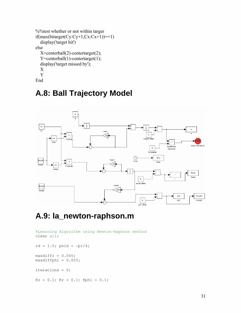
In order to test the two different algorithms, a physics model was created to simulate the motion of the ping pong ball as affected by disturbance (air friction, spin). The model was based on basic projectile physics with the addition of three coefficients, two of which simulate air friction and the third adds a “spin” disturbance. Two coefficients (Kz and Kr) attenuate the velocity of the r and z axis as shown in equations 24 and 25. The third coefficient (Kφ) creates a “spin” by attenuating the φ coordinate as shown in equation (26). The model can be seen in Appendix A.8 and the two M-files used to simulate each algorithm can be found in Appendix A.9 and A.10. [2]

( 1) 0 1 ( )sinz k z z kV V K V+ = Θ − (24)

16

( 1) 0 1 ( )cosr k r r kV V K V+ = Θ − (25)

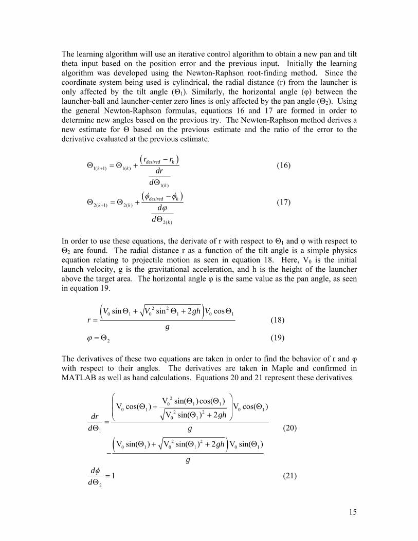
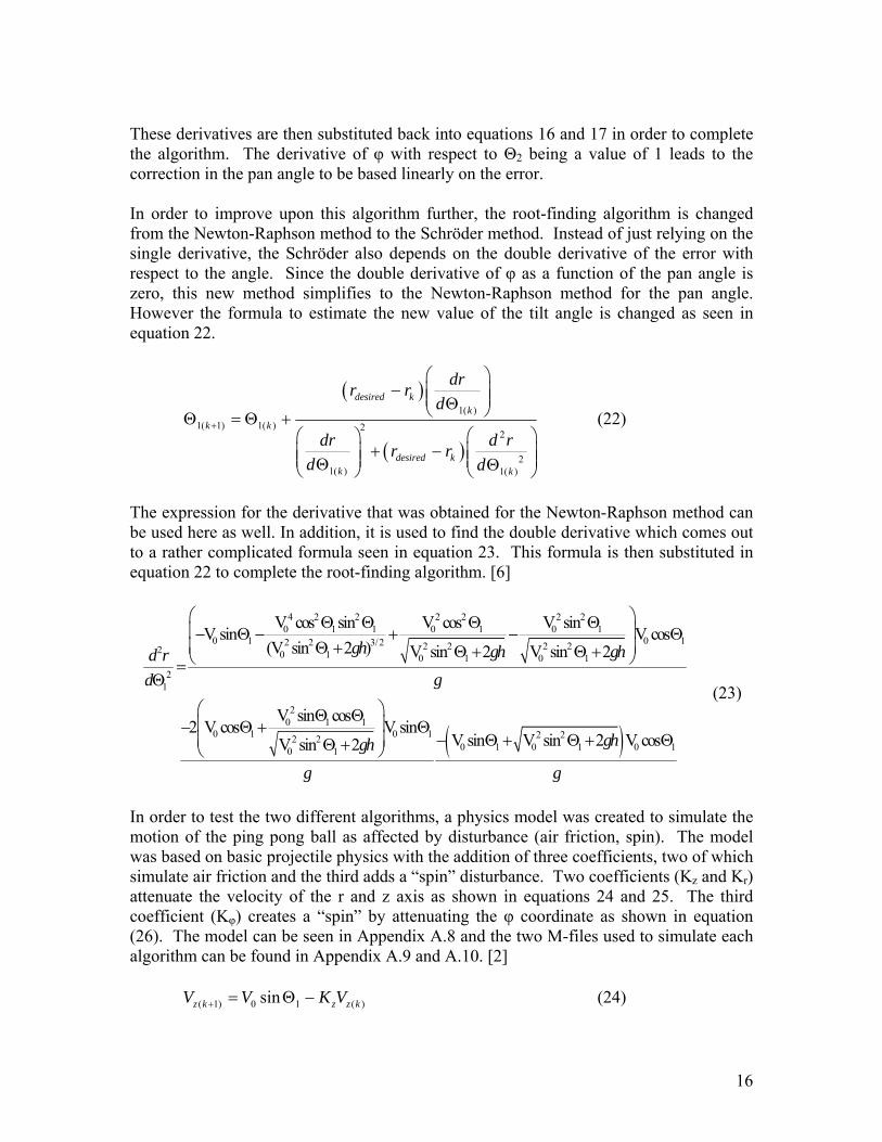
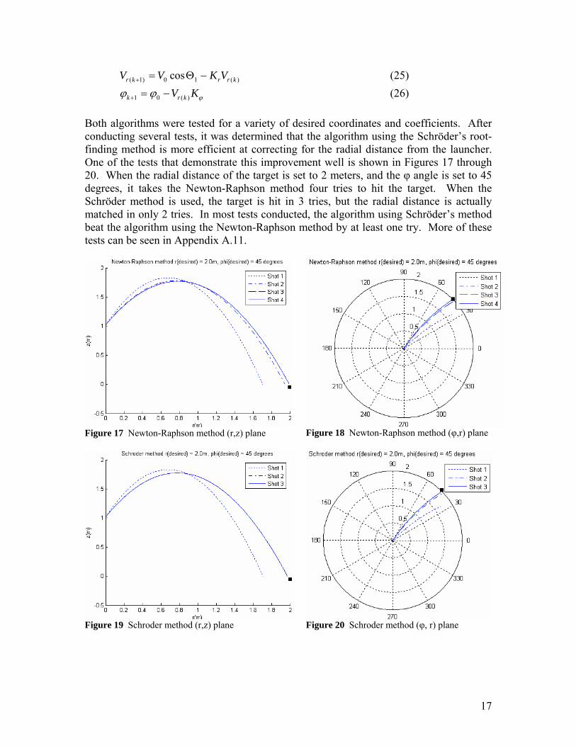
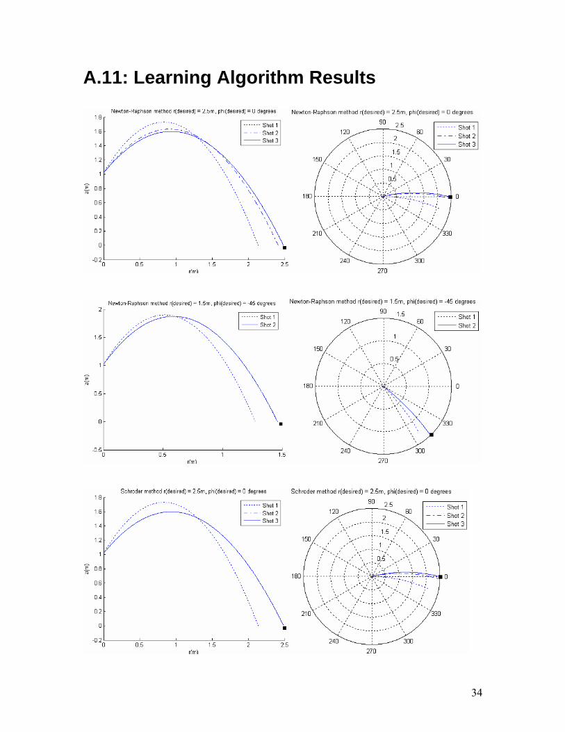
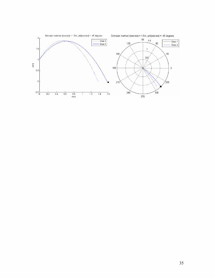
1 0 ( )k rV Kk ϕϕ ϕ+ = − (26) Both algorithms were tested for a variety of desired coordinates and coefficients. After conducting several tests, it was determined that the algorithm using the Schröder’s root-finding method is more efficient at correcting for the radial distance from the launcher. One of the tests that demonstrate this improvement well is shown in Figures 17 through 20. When the radial distance of the target is set to 2 meters, and the φ angle is set to 45 degrees, it takes the Newton-Raphson method four tries to hit the target. When the Schröder method is used, the target is hit in 3 tries, but the radial distance is actually matched in only 2 tries. In most tests conducted, the algorithm using Schröder’s method beat the algorithm using the Newton-Raphson method by at least one try. More of these tests can be seen in Appendix A.11.

Figure 17 Newton-Raphson method (r,z) plane

Figure 18 Newton-Raphson method (φ,r) plane

Figure 19 Schroder method (r,z) plane

Figure 20 Schroder method (φ, r) plane

17

Thus the Schröder method was chosen to be implemented when the algorithm is integrated with the rest of the machine. The number of attempts to hit the target never exceeded four using either of the two algorithms. Assuming correct functionality of the rest of the mechanism, these tests ensure that the learning algorithm should be able to hit the target within the eight attempts specified in the project proposal.

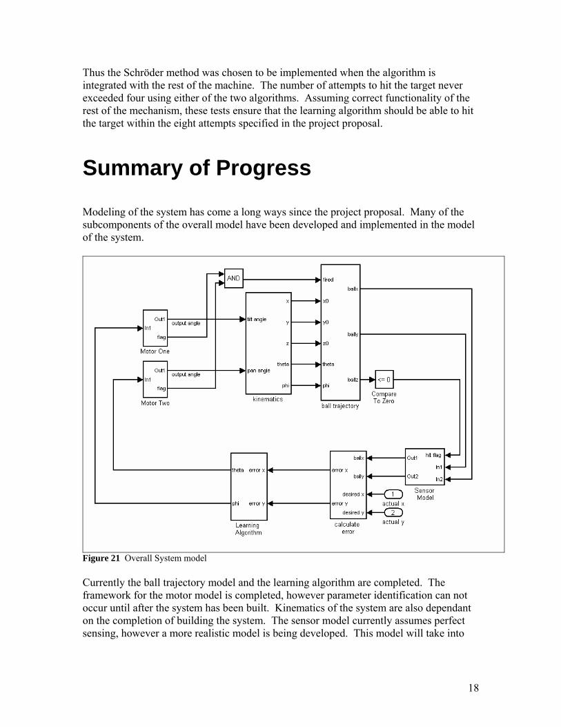
Summary of Progress Modeling of the system has come a long ways since the project proposal. Many of the subcomponents of the overall model have been developed and implemented in the model of the system.

Figure 21 Overall System model Currently the ball trajectory model and the learning algorithm are completed. The framework for the motor model is completed, however parameter identification can not occur until after the system has been built. Kinematics of the system are also dependant on the completion of building the system. The sensor model currently assumes perfect sensing, however a more realistic model is being developed. This model will take into

18

account the limited visibility of the webcam, possible processing delays, and sensor noise. At this point we were scheduled to have completed parameter identification, model verification, and start of controller design. Due to the fact that our system is still not completely built, these parameters do not yet exist and thus parameter identification can not take place. Since there is no physical system in place to compare the model to, model verification is also not possible. However, these setbacks have not halted productivity. An algorithm was developed and tested on a model to identify the parameters of the model. This algorithm is also self verifying because based on the resulting Eigen values the accuracy of these parameters can be determined. Initial control design has also taken place. Using estimated values for inertia and other parameters a controller was designed to generate a response for the tilt motor with almost no overshoot, a rise time of less than one second, and fast settling time. According to the schedule that we created for the project proposal, the launching system had three main tasks scheduled to be done before the current date. These are accuracy testing of the gun, gun modification as needed and further testing, and the mounting of the gun onto the pan-tilt device. Because of the difficulties we had with pressure build up, we had to rethink our plan before it was possible to test the system for accuracy. We did some extensive modifications to the gun in order to get it working, as described in the preliminary results section. Therefore we consider this task to have been fulfilled, although there may be some future modification necessary. Because of this delay our accuracy testing is way behind schedule. We have not yet taken any analytical measurements as to the accuracy of the gun given the current setup. This is something which will be done as soon as possible. The third task that needed to be completed was the mounting of the gun onto the pan-tilt device. This is also slightly behind schedule, although we have fully developed a plan for this task and have purchased the parts necessary for this plan. All that is left to do is to implement the plan, so this task is not too far behind schedule. The details of the gun mounting are described in an earlier section of this report. The challenges to the construction of the launcher are described in the preliminary results section. I will summarize them here. First, an electronically controlled valve and launcher body needed to be acquired. This was done by ordering the valve and a ping pong ball gun online, and making modifications to the ping pong ball gun. Next was the issue of attaching the valve to the air tank in the lab. A barb was purchased to screw into the inlet of the valve. Tubing was purchased to attach to this barb and run to the air tank in the lab. Because the barb only supports 1/8 in. diameter tubing and the air tank needs 3/8 in. diameter tubing, a device was purchased to step up from the smaller tuning size to the larger. The larger tubing did not need to be bought because there was some free for use in the lab. After this it was necessary to attach the valve to the gun. A tap was used to bore a threaded hole into the back of the launcher, and the same size barb that the valve uses

19

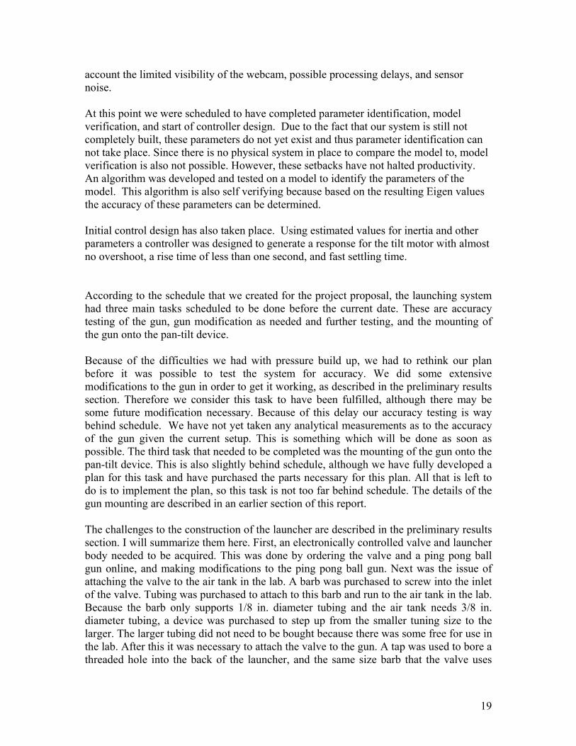
was placed into this launcher. It was then possible to use one tube to connect the two. The last challenge was to remove the pressure build up which was causing tubing to come loose. This was done by reworking our design so that the airflow splits, and the valve controls whether the air goes to the launcher or flows freely into the room (instead of just building up in the tubing as with our previous design). For the remainder of the project we have the following tasks for the launching system. First comes the mounting of the gun onto the pan-tilt. Second we will test for accuracy and to get an uncertainty measurement of the launched balls. Our launcher fires balls a little too fast for our convenience, so if possible we will then develop a plan to modify the nozzle of the gun or to modify the balls used. This will bring the initial velocity down to a more desirable value. If this is done we will retest for accuracy. Another challenge is integrating the launcher with the controller, i.e, how exactly do we wire the electronic valve to our system so that it can be controlled by our code. This is a very important step and so it will also be one of the first things taken care of. After this the launching system will be complete, unless any further problems arise. Progress on the feedback has been temporary put on hold due to more pressing matters. As of right now the team has the means to mount the camera above the target. The algorithm to determine the success of a launch is completed. The integration of the piezo devices and the camera is yet to be completed. Also the timing of the camera with respect to the ball launch and piezo devices needs to be completed. The cost estimate of the feedback system in the project proposal has been accurate. Until the launcher mounting issues are resolved progress on the feedback system is put on hold. The preliminary design of the launcher mount has been completed. The launcher mounting needs to be built and tested. In the previous report no considerations for the cost of the mounting was addressed. All the materials to build the mount have been purchased and came to $24.68. The mount should be built by April 2nd. The learning algorithm cannot proceed further until the rest of the system is integrated. Both Newton-Raphson and Schröder methods were derived and simulated based on our physics model of the ball trajectory. The Schröder algorithm was chosen to be implemented in the final machine due to its increased efficiency. The simulated results show a worst case scenario of four tries to hit the target. This is well within the proposed goal of hitting the target within eight tries. However, tuning still needs to be done after the algorithm is integrated, to account for unexpected gains and offsets. The algorithm is still based only on MATLAB/Simulink and has not incurred any additional costs. A new schedule has been developed based on our current progress, and is shown in Figure 22.

20

Figure 22 Schedule

21

Bibliography 1. Franklin, G.F., J.D. Powell, and A. Emami-Naeini, Feedback Control of Dynamic Systems, 4th Edition, Addison-Wesley, 2002. 2. Weisstein, Eric W. “Drag Coefficient”. Internet. (2005) Available: http://scienceworld.wolfram.com/physics/DragCoefficient.html, Feb. 2005. 3. Wen, John T. “ECSE 4460 Control System Design, Spring 2005”. Internet. (2005) Available: http://www.cat.rpi.edu/~wen/ECSE446S05/identification.pdf, Feb. 2005. 4. “Ball-Shooting Burp Gun”. Internet. (2005) Available: http://amos.shop.com/amos/cc/pcd/4614366/prd/6715663/ccsyn/260, Feb. 2005. 5. “DC Motor Specifications Sheet”. Internet. (2002) Available: http://www.pennmotion.com/pdf/lcg_bulletin.pdf, Feb. 2005. 6. “Root-Finding”. Internet. (2004) Available: http://mathworld.wolfram.com/topics/Root-Finding.html, Feb. 2005. 7. “The Proportional Valve”. Internet. (2005) Available: http://www.clippard.com/store/byo_electronic/byo_proportional_valves.asp, Feb. 2005.

22

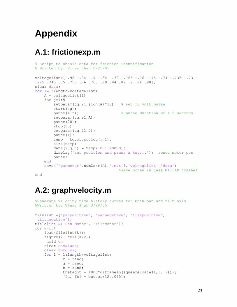
Appendix A.1: frictionexp.m % Script to obtain data for friction identification % Written by: Vinay Shah 2/25/05 voltagelist=[-.98 -.94 -.9 -.84 -.79 -.765 -.76 -.75 -.74 -.735 -.73 -.725 .745 .75 .755 .76 .765 .79 .84 .87 .9 .94 .98]; clear data; for i=1:length(voltagelist) A = voltagelist(i) for j=1:5 setparam(tg,21,sign(A)*10); % set 10 volt pulse start(tg); pause(1.5); % pulse duration of 1.5 seconds setparam(tg,21,A); pause(20); stop(tg); setparam(tg,21,0); pause(1); temp = tg.outputlog(:,1); size(temp) data(i,j,:) = temp(1001:20000); display('set position and press a key...'); reset motor pos pause; end save(['panmotor',num2str(A),'.mat'],'voltagelist','data')

%save often in case MATLAB crashes end

A.2: graphvelocity.m %Generate velocity time history curves for both pan and tilt axis %Written by: Vinay Shah 3/28/05 filelist ={'panpositive', 'pannegative', 'tiltpositive', 'tiltnegative'}; titlelist ={'Pan Motor', 'Tiltmotor'}; for k=1:4 load(filelist{k}); figure(2+ ceil(k/2)) hold on clear ssvalues; clear torques; for i = 1:length(voltagelist) r = rand; g = rand; b = rand; thetadot = 1000*diff(mean(squeeze(data(i,:,:)))); [fa, fb] = butter(12,.065);

23

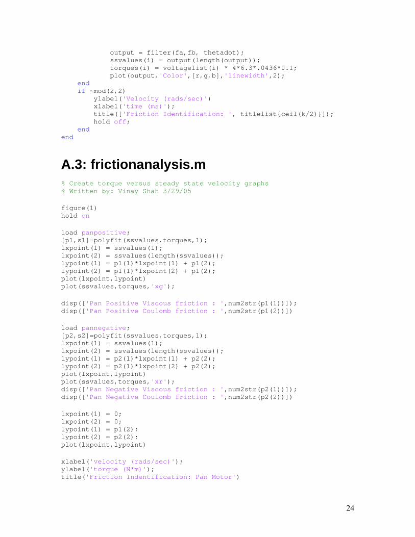
output = filter(fa,fb, thetadot); ssvalues(i) = output(length(output)); torques(i) = voltagelist(i) * 4*6.3*.0436*0.1; plot(output,'Color',[r,g,b],'linewidth',2); end if ~mod(2,2) ylabel('Velocity (rads/sec)') xlabel('time (ms)'); title(['Friction Identification: ', titlelist{ceil(k/2)}]); hold off; end end

A.3: frictionanalysis.m % Create torque versus steady state velocity graphs % Written by: Vinay Shah 3/29/05 figure(1) hold on load panpositive; [p1,s1]=polyfit(ssvalues,torques,1); lxpoint(1) = ssvalues(1); lxpoint(2) = ssvalues(length(ssvalues)); lypoint(1) = p1(1)*lxpoint(1) + p1(2); lypoint(2) = p1(1)*lxpoint(2) + p1(2); plot(lxpoint,lypoint) plot(ssvalues,torques,'xg'); disp(['Pan Positive Viscous friction : ',num2str(p1(1))]); disp(['Pan Positive Coulomb friction : ',num2str(p1(2))]) load pannegative; [p2,s2]=polyfit(ssvalues,torques,1); lxpoint(1) = ssvalues(1); lxpoint(2) = ssvalues(length(ssvalues)); lypoint(1) = p2(1)*lxpoint(1) + p2(2); lypoint(2) = p2(1)*lxpoint(2) + p2(2); plot(lxpoint,lypoint) plot(ssvalues,torques,'xr'); disp(['Pan Negative Viscous friction : ',num2str(p2(1))]); disp(['Pan Negative Coulomb friction : ',num2str(p2(2))]) lxpoint(1) = 0; lxpoint(2) = 0; lypoint(1) = p1(2); lypoint(2) = p2(2); plot(lxpoint,lypoint) xlabel('velocity (rads/sec)'); ylabel('torque (N*m)'); title('Friction Indentification: Pan Motor')

24

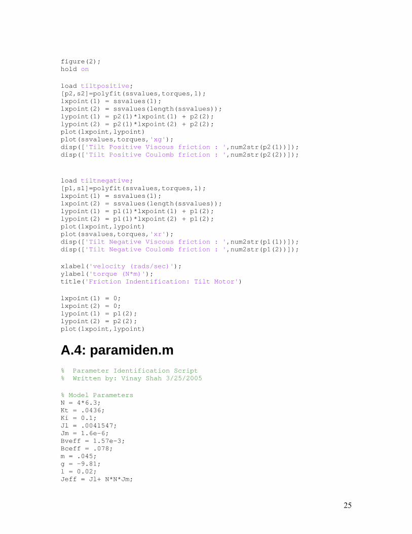
figure(2); hold on load tiltpositive; [p2,s2]=polyfit(ssvalues,torques,1); lxpoint(1) = ssvalues(1); lxpoint(2) = ssvalues(length(ssvalues)); lypoint(1) = p2(1)*lxpoint(1) + p2(2); lypoint(2) = p2(1)*lxpoint(2) + p2(2); plot(lxpoint,lypoint) plot(ssvalues,torques,'xg'); disp(['Tilt Positive Viscous friction : ',num2str(p2(1))]); disp(['Tilt Positive Coulomb friction : ',num2str(p2(2))]); load tiltnegative; [p1,s1]=polyfit(ssvalues,torques,1); lxpoint(1) = ssvalues(1); lxpoint(2) = ssvalues(length(ssvalues)); lypoint(1) = p1(1)*lxpoint(1) + p1(2); lypoint(2) = p1(1)*lxpoint(2) + p1(2); plot(lxpoint,lypoint) plot(ssvalues,torques,'xr'); disp(['Tilt Negative Viscous friction : ',num2str(p1(1))]); disp(['Tilt Negative Coulomb friction : ',num2str(p1(2))]); xlabel('velocity (rads/sec)'); ylabel('torque (N*m)'); title('Friction Indentification: Tilt Motor') lxpoint(1) = 0; lxpoint(2) = 0; lypoint(1) = p1(2); lypoint(2) = p2(2); plot(lxpoint,lypoint)

A.4: paramiden.m % Parameter Identification Script % Written by: Vinay Shah 3/25/2005 % Model Parameters N = 4*6.3; Kt = .0436; Ki = 0.1; Jl = .0041547; Jm = 1.6e-6; Bveff = 1.57e-3; Bceff = .078; m = .045; g = -9.81 ;l = 0.02; Jeff = Jl+ N*N*Jm;

25

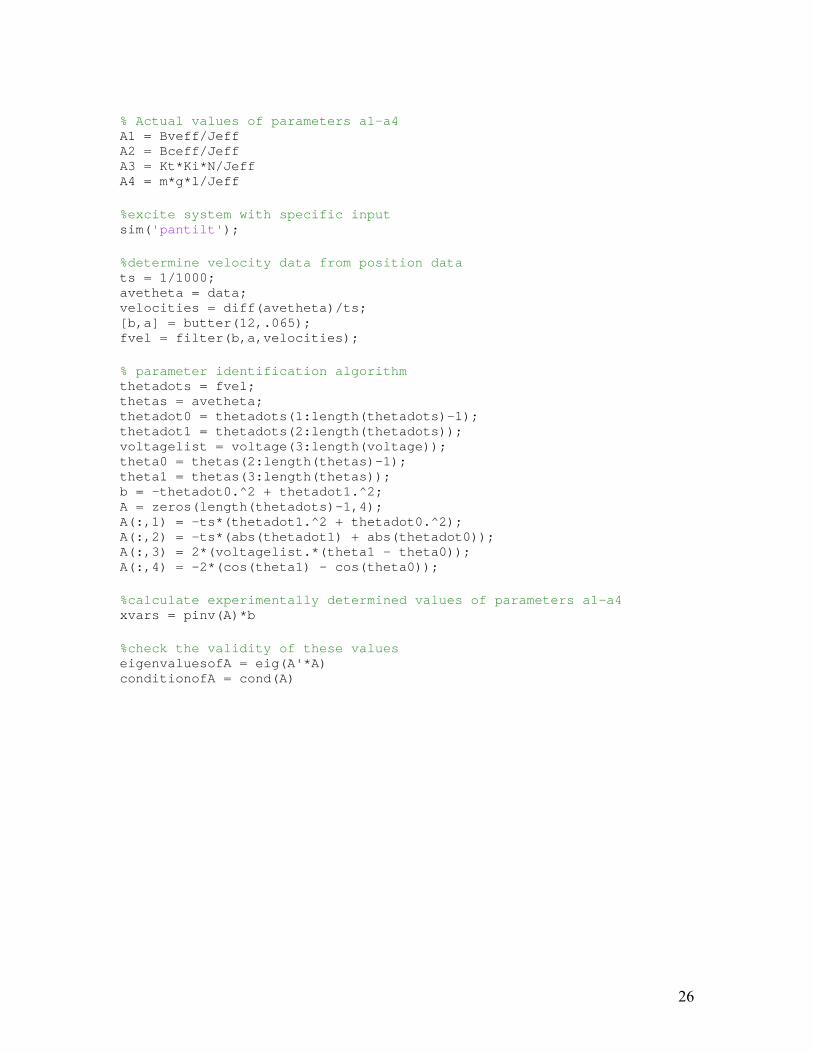
% Actual values of parameters a1-a4 A1 = Bveff/Jeff A2 = Bceff/Jeff A3 = Kt*Ki*N/Jeff A4 = m*g*l/Jeff %excite system with specific input sim('pantilt'); %determine velocity data from position data ts = 1/1000; avetheta = data; velocities = diff(avetheta)/ts; [b,a] = butter(12,.065); fvel = filter(b,a,velocities); % parameter identification algorithm thetadots = fvel; thetas = avetheta; thetadot0 = thetadots(1:length(thetadots)-1); thetadot1 = thetadots(2:length(thetadots)); voltagelist = voltage(3:length(voltage)); theta0 = thetas(2:length(thetas)-1); theta1 = thetas(3:length(thetas)); b = -thetadot0.^2 + thetadot1.^2; A = zeros(length(thetadots)-1,4); A(:,1) = -ts*(thetadot1.^2 + thetadot0.^2); A(:,2) = -ts*(abs(thetadot1) + abs(thetadot0)); A(:,3) = 2*(voltagelist.*(theta1 - theta0)); A(:,4) = -2*(cos(theta1) - cos(theta0)); %calculate experimentally determined values of parameters a1-a4 xvars = pinv(A)*b %check the validity of these values eigenvaluesofA = eig(A'*A) conditionofA = cond(A)

26

A.5: Processing Algorithm

Target Area

Image of Target

Location of Target

Camera Binarization

Center of Target

Ball hits piezo device

Camera

Color image of ball location

Binarization

Noise Reduction

Center of Ball

Comparison Inside target

Successful Unsuccessful

Convert ball location to world coordinates

Learning Algorithm

27

A.6: Feedback System

Camera

Frame

A.7: Feedback MATLAB Code function D=thresh(image,k1,k2) %%image is rgb %%set k1 and k2 to adjust for outside interference %%k1+k2=2, k1 increases background, k2 increases foreground %%returns bilevel image global s; image=rgb2gray(image); %%convert to greyscale s=size(image); m0=50; %%initial guesses m1=125; Tp=200; T=87; while(Tp~=T) %%interative algorithm to find threshold Tp=T; fore=0; back=0; f=0; b=0; for(i=1:s(1)) for(j=1:s(2)) V=double(image(i,j)); if(image(i,j)<=T) fore=fore+V;

Piezo Devices

Amplifier XPC Target

Ball Lands

Laptop

Image Processing

Coordinates Learning Algorithm

28

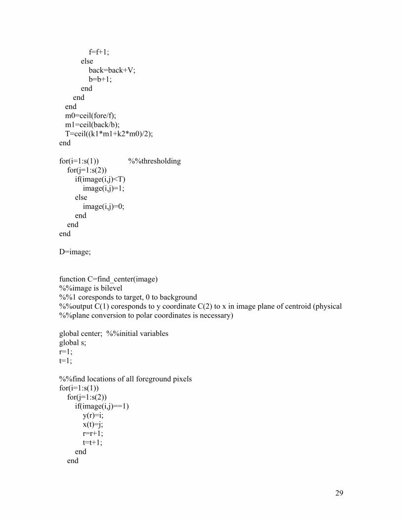
f=f+1; else back=back+V; b=b+1; end end end m0=ceil(fore/f); m1=ceil(back/b); T=ceil((k1*m1+k2*m0)/2); end for(i=1:s(1)) %%thresholding for(j=1:s(2)) if(image(i,j)<T) image(i,j)=1; else image(i,j)=0; end end end D=image; function C=find_center(image) %%image is bilevel %%1 coresponds to target, 0 to background %%output C(1) coresponds to y coordinate C(2) to x in image plane of centroid (physical %%plane conversion to polar coordinates is necessary) global center; %%initial variables global s; r=1; t=1; %%find locations of all foreground pixels for(i=1:s(1)) for(j=1:s(2)) if(image(i,j)==1) y(r)=i; x(t)=j; r=r+1; t=t+1; end end

29

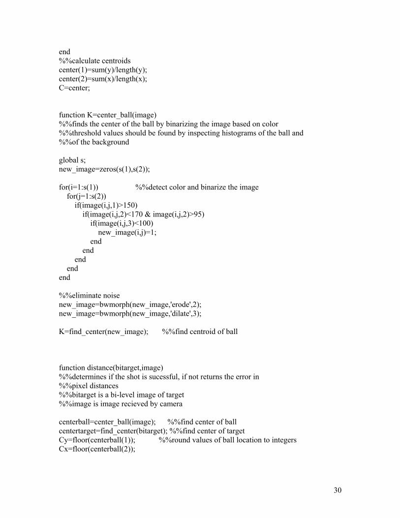
end %%calculate centroids center(1)=sum(y)/length(y); center(2)=sum(x)/length(x); C=center; function K=center_ball(image) %%finds the center of the ball by binarizing the image based on color %%threshold values should be found by inspecting histograms of the ball and %%of the background global s; new_image=zeros(s(1),s(2)); for(i=1:s(1)) %%detect color and binarize the image for(j=1:s(2)) if(image(i,j,1)>150) if(image(i,j,2)<170 & image(i,j,2)>95) if(image(i,j,3)<100) new_image(i,j)=1; end end end end end %%eliminate noise new_image=bwmorph(new_image,'erode',2); new_image=bwmorph(new_image,'dilate',3); K=find_center(new_image); %%find centroid of ball function distance(bitarget,image) %%determines if the shot is sucessful, if not returns the error in %%pixel distances %%bitarget is a bi-level image of target %%image is image recieved by camera centerball=center_ball(image); %%find center of ball centertarget=find_center(bitarget); %%find center of target Cy=floor(centerball(1)); %%round values of ball location to integers Cx=floor(centerball(2));

30

%%test whether or not within targer if(max(bitarget(Cy:Cy+1,Cx:Cx+1))==1) display('target hit') else X=centerball(2)-centertarget(2); Y=centerball(1)-centertarget(1); display('target missed by'); X Y End

A.8: Ball Trajectory Model

A.9: la_newton-raphson.m %Learning Algorithm using Newton-Raphson method clear all; rd = 1.5; phid = -pi/4; maxdiffr = 0.045; maxdiffphi = 0.025; iterations = 0; Kz = 0.1; Kr = 0.1; Kphi = 0.1;

31

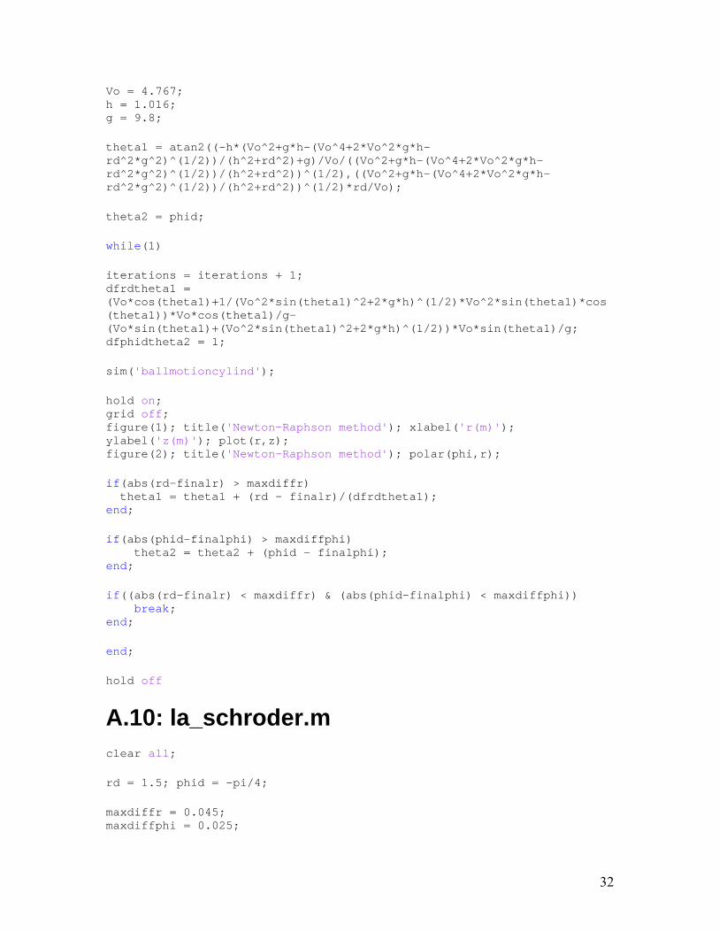
Vo = 4.767; h = 1.016; g = 9.8; theta1 = atan2((-h*(Vo^2+g*h-(Vo^4+2*Vo^2*g*h-rd^2*g^2)^(1/2))/(h^2+rd^2)+g)/Vo/((Vo^2+g*h-(Vo^4+2*Vo^2*g*h-rd^2*g^2)^(1/2))/(h^2+rd^2))^(1/2),((Vo^2+g*h-(Vo^4+2*Vo^2*g*h-rd^2*g^2)^(1/2))/(h^2+rd^2))^(1/2)*rd/Vo); theta2 = phid; while(1) iterations = iterations + 1; dfrdtheta1 = (Vo*cos(theta1)+1/(Vo^2*sin(theta1)^2+2*g*h)^(1/2)*Vo^2*sin(theta1)*cos(theta1))*Vo*cos(theta1)/g-(Vo*sin(theta1)+(Vo^2*sin(theta1)^2+2*g*h)^(1/2))*Vo*sin(theta1)/g; dfphidtheta2 = 1; sim('ballmotioncylind'); hold on; grid off; figure(1); title('Newton-Raphson method'); xlabel('r(m)'); ylabel('z(m)'); plot(r,z); figure(2); title('Newton-Raphson method'); polar(phi,r); if(abs(rd-finalr) > maxdiffr) theta1 = theta1 + (rd - finalr)/(dfrdtheta1); end; if(abs(phid-finalphi) > maxdiffphi) theta2 = theta2 + (phid - finalphi); end; if((abs(rd-finalr) < maxdiffr) & (abs(phid-finalphi) < maxdiffphi)) break; end; end; hold off

A.10: la_schroder.m clear all; rd = 1.5; phid = -pi/4; maxdiffr = 0.045; maxdiffphi = 0.025;

32

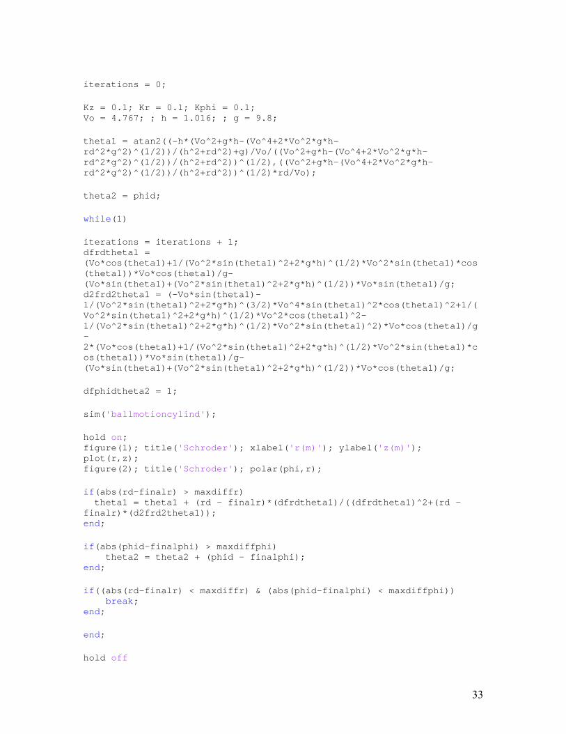
iterations = 0; Kz = 0.1; Kr = 0.1; Kphi = 0.1; Vo = 4.767; ; h = 1.016; ; g = 9.8; theta1 = atan2((-h*(Vo^2+g*h-(Vo^4+2*Vo^2*g*h-rd^2*g^2)^(1/2))/(h^2+rd^2)+g)/Vo/((Vo^2+g*h-(Vo^4+2*Vo^2*g*h-rd^2*g^2)^(1/2))/(h^2+rd^2))^(1/2),((Vo^2+g*h-(Vo^4+2*Vo^2*g*h-rd^2*g^2)^(1/2))/(h^2+rd^2))^(1/2)*rd/Vo); theta2 = phid; while(1) iterations = iterations + 1; dfrdtheta1 = (Vo*cos(theta1)+1/(Vo^2*sin(theta1)^2+2*g*h)^(1/2)*Vo^2*sin(theta1)*cos(theta1))*Vo*cos(theta1)/g-(Vo*sin(theta1)+(Vo^2*sin(theta1)^2+2*g*h)^(1/2))*Vo*sin(theta1)/g; d2frd2theta1 = (-Vo*sin(theta1)-1/(Vo^2*sin(theta1)^2+2*g*h)^(3/2)*Vo^4*sin(theta1)^2*cos(theta1)^2+1/(Vo^2*sin(theta1)^2+2*g*h)^(1/2)*Vo^2*cos(theta1)^2-1/(Vo^2*sin(theta1)^2+2*g*h)^(1/2)*Vo^2*sin(theta1)^2)*Vo*cos(theta1)/g-2*(Vo*cos(theta1)+1/(Vo^2*sin(theta1)^2+2*g*h)^(1/2)*Vo^2*sin(theta1)*cos(theta1))*Vo*sin(theta1)/g-(Vo*sin(theta1)+(Vo^2*sin(theta1)^2+2*g*h)^(1/2))*Vo*cos(theta1)/g; dfphidtheta2 = 1; sim('ballmotioncylind'); hold on; figure(1); title('Schroder'); xlabel('r(m)'); ylabel('z(m)'); plot(r,z); figure(2); title('Schroder'); polar(phi,r); if(abs(rd-finalr) > maxdiffr) theta1 = theta1 + (rd - finalr)*(dfrdtheta1)/((dfrdtheta1)^2+(rd - finalr)*(d2frd2theta1)); end; if(abs(phid-finalphi) > maxdiffphi) theta2 = theta2 + (phid - finalphi); end; if((abs(rd-finalr) < maxdiffr) & (abs(phid-finalphi) < maxdiffphi)) break; end; end; hold off

33

A.11: Learning Algorithm Results

34

35

Statement of Contribution All team members worked equally in the production of this report. Once again each team member wrote about their own system. Larry Cole worked on the feedback system, launcher mounting, and schedule. Vinay Shah worked on the system model, controller, and abstract. Danish Zia worked on the learning algorithm, bibliography, and appendix. Bert Hallonquist worked on the launcher assembly and introduction. __________________________ ________________________ Larry Cole Vinay Shah __________________________ ________________________ Danish Zia Bert Halloquist

36