Beirut Master 4000 Project Proposal ECSE-4460 Control System Design

Team 2 Larry Cole Vinay Shah Danish Zia

Bert Hallonquist

Wednesday, March 2, 2005

Rensselaer Polytechnic Institute

ii

Abstract This document proposes a design project which will attempt to successfully launch a ball into a cup. By mounting a pneumatic launcher on a pan and tilt mechanism a ping pong ball can be launched to within a range of locations. Solutions for pan and tilt angles which successfully place the ball in the cup will be determined by an iterative learning algorithm. A controller will be designed through the use of experimentation, modeling, and simulation to quickly command the motor to the desired location. An automated feedback system will be developed using a camera coupled with image processing. The overall goal of this project is to design an automated system to quickly place a ball in a cup my minimizing the time it takes to position the launcher and the number of iterations required to converge to the solution.

1

Contents Table of Contents Introduction.........................................................................................................3 Objectives............................................................................................................4 Design Strategy...................................................................................................5 Motor Control ..................................................................................................5 Launcher System ............................................................................................8 Feedback System............................................................................................8 Learning Algorithm.......................................................................................15 Plan of Action....................................................................................................17 Motor control.................................................................................................17 Launching System ........................................................................................18 Feedback System..........................................................................................18 Learning Algorithm.......................................................................................18 Verification ........................................................................................................17 Motor control.................................................................................................17 Launching System ........................................................................................17 Feedback System..........................................................................................17 Learning Algorithm.......................................................................................23 Tolerance Analysis ...........................................................................................26 Cost and Schedule............................................................................................26 Bibliography......................................................................................................29 Appendix ...........................................................................................................32 Table of Figures Figure 1 System Overview ................................................................................6 Figure 2 DC Motor Model ..................................................................................6 Figure 3 Friction Identification..........................................................................7 Figure 4 PASCO Projectile Launcher ...............................................................9 Figure 5 GUNT projectile launcher ...................................................................9 Figure 6 Ping pong ball gun............................................................................10 Figure 7 Experiment using spring loaded launcher......................................10 Figure 8 Experiment using compressed air launcher...................................11 Figure 9 Some Valve dimensions....................................................................12 Figure 10 Outside view of proposed valve. ...................................................12 Figure 11 A USB web-cam. .............................................................................13 Figure 12 Learning Algorithm Block Diagram...............................................16 Figure 13 Test target.........................................................................................21 Figure 14 Histogram of test area ....................................................................21 Figure 15 Target area.......................................................................................22 Figure 16 Color histograms of background...................................................23 Figure 17 Color histograms of ball.................................................................23

2

Figure 18 Original image .................................................................................24 Figure 19 Bi-level ball image before processing...........................................24 Figure 20 Bi-level ball image after processing..............................................25

3

Introduction

We are attempting to create a machine which is capable of playing the game of “Beirut” automatically. Beirut is a game where the player attempts to throw a ping pong ball into a cup which is a short distance away from the player. It is quite clear then that our machine will need to have some means of throwing, shooting, or otherwise projecting a ball towards a cup. The launching system will be mounted on the pan-and-tilt device. This will allow us to change the direction of the launcher and thus change the trajectory of the projectile as desired. After the projectile has been fired, the system will then need some sensory equipment in order to detect the location of the ball as compared to the target cup in the base coordinate frame. The data retrieved from this feedback system will need to be sent to a controller to be manipulated. This controller will determine the error between the actual output ball location and the desired ball location. Using this error signal the controller will determine a new set of pan and tilt angles to position the launcher. This controller will use an iterative learning algorithm to calculate the adjustments that need to be made. Another controller will be implemented to “smooth” out the response of the motors that drive the pan-and-tilt device. This means making sure that the motors don’t become unstable, their response is fast, and there is zero steady state error between the actual and desired motor output. In addition to this, the controller will be sending signals to the launcher, telling it when to fire again. Using this type of system, the learning algorithm and controller will cause the launched ball to come closer and closer to striking the target. After a certain number of iterations the launcher should be able to strike the target consistently. The development of an iterative learning algorithm has applications outside the scope of the game of Beirut. The military, for example, might be interested in such and algorithm for firing missiles. The robotics industry is constantly looking for ways to develop artificial intelligence for their products. An algorithm like this might be used to help robots become more aware of their surroundings by learning how to judge distances.

4

Objectives The goal of this project is to hit a target with a projectile. The first challenge will be in launching the ball. The ball launcher must be both accurate and repeatable. Initially the team used a foam disk launcher, but it lacked the accuracy and repeatability needed for a successful project. The team will use an air powered ping pong ball launcher. The launcher will be mounted on a pan-tilt mechanism. The launcher should not weigh down the system. The pan-tilt mechanism will be controlled by either a PID, finite settling time, or a full state feedback controller. Since the shooter will have time between attempts overshoot and rise time will not be as important as in other applications. The settling time will be minimized be less than 0.5 seconds to speed up the process of the system. If the system is to be applied for military use, and the target was the enemy, if the system takes a long time the enemy might have a chance to escape or conduct a counterattack. When the projectile is launched, the location of where it hits must be recorded. Initially the target was to be raised above the ground and 2 web cams were to be used to record the ball location. This approach was abandoned due to challenges that would arise with synchronizing two cameras. The location will be recorded by using a single webcam and a trigger. The challenge with this approach will be synchronizing the trigger with the camera. After the location is stored, a learning algorithm will determine the angle for the next launch. Then the entire process is repeated, with new launch angles. The algorithm must be designed so that the number of iterations is minimized. If the system is to be implemented for a military applications, missing the target will give away your location. The goal is to place the ball into the cup within 8 iterations.

5

Design Strategy Due to the complexity of the project, the design will be split into four sections, motor control, feedback system, learning algorithm, and the launcher subsystem. The design strategy of overall system as well as each subsection will be comprised of modeling, parameter identification, simulation, validation, control design, and performance verification. A model of the overall system was developed and is displayed below:

Figure 1 System Overview

The advantage of developing a model is that rather than running experiments, which can be long and require a great deal of setup, simulations can be ran and results obtained faster with no setup. One necessary parameter is the drag coefficient on the ping pong ball which is used for modeling the ball trajectory. This was calculated for a smooth ping pong ball in [8 ] to be .00238 m/s. In order to simulate the overall model each subsystem must be accurately modeled. Each subsystem will be designed using a similar approach. Motor Control

6

A model of the motor is required for designing a controller for motor control. The standard model for a dc motor is of the following form [5]:

1

Out1

1

Jeff1.s+Beff1

load

-K-

back emf

n1

s-K-

Motor Torque Constant

1

L1.s+R1

Motor Armature

1

In1output angle

Figure 2 DC Motor Model

L1 and R1 refer to the motor’s inductance and resistance, Jeff and Beff is the effective inertia and friction, n1 represents the gear ratio. Non-linearities such as saturation and quantization also occur but will be ignored in order to design the controller. Typical value of the parameters required to model the motor can be found in the motor’s spec sheet [11]. However, to obtain a more accurate model experimentation is required to determine the actual parameters for the given motors. This will be done in the system identification stage. A dynamic model of the system will be modeled using the Langrange-Euler equation. This equation will provide the torque seen at the two joints of our system. Similar to the motor model, parameters will need to be identified to complete the model. Necessary parameters include mass, gravity loading, friction, inertia tensor, center of gravity, and velocity coupling [5]. In order to accurately model our system many parameters need to be determined either experimentally or empirically. For example, in determining viscous and coulomb friction we first assumed that friction and velocity have the following relationship:

)sgn(AFFA cv += θ� (1)

A is a constant torque and θ� is the steady state velocity. This may not be a completely accurate representation of friction, however it serves as an adequate model. By applying a constant torque, A, into the system and plotting the output, the viscous and coulomb friction can be observed directly from the plot as the slope and y intercept respectively. A MATLAB script was written to run an experiment which generated various torques (by inputting various voltages to the motor) and recorded the steady state velocity. The experiment ran five times for each torque and the steady state velocity was averaged for the 5 runs. Blow is a result from our initial experimentation:

7

-25 -20 -15 -10 -5 0 5 10 15 20 25-10

-5

0

5

10

theta dot (deg/sec)

Inpu

t Vol

tage

(V)

Friction Identification Motor 1

-20 -15 -10 -5 0 5 10 15 20 25-10

-5

0

5

10

theta dot (deg/sec)

Inpu

t Vol

tage

(V)

Friction Identification Motor 2

Figure 3 Friction Identification

Torque is related to the voltage by the following equation:

Torque = (voltage)* internal gear ratio)*torque constant* Amplifier gain. (2)

The external gear ratio is 4 [7], the internal gear ratio is 6.31, the torque constant is found in the data sheet as .0291 N*m/A [7] and the amplifier gain is set as 0.1 [9]. Thus the torque = 0.07345 *voltage. Saturation occurred in the initial experiment and thus the experiment will need to be rerun while recording more data points prior to velocity saturation. Once accurate data is measured, two linear regressions, one for positive torques and another for negative torques, can be made to model friction. As mentioned above, the slope of the line will be the viscous friction while the intercept will be the coulomb friction. Solidworks can be used to develop a model of the physical structure of the system which can be used to determine parameters such as mass and center of gravity. Further experiments will be designed for determining parameters such as the inertia tensor, gravity loading, and velocity coupling matrices. Once the model is complete, its open loop response should be compared with that of the actual plant. One method of doing this would be to supply a random input and see how well the output of the model matches that of the plant. However, since our project is only

8

concerned with a step response, the verification process should only analyze any differences in the step response of the model and the plant. When verifying the model, non-linearities such as saturation, quantization, and friction modeling should be incorporated in the model. Once the model adequately matches the plant, design of the controller may begin. The controller will be designed such that the there is a settling time of less than 0.5 seconds and zero steady state error. There is no desired overshoot specification, as overshoot is not an issue for our purposes, however it should be within an acceptable range. There are many different types of controller design methods which can be employed. The classical approach is to use a PID controller. To begin the process the model must be linearized. Root locus analysis will be used to determine values for the proportional, derivative, and integral gains. Another controller would be a full state feedback controller. This approach places state variables in the feedback loop which allows the poles of the system to be moved to locations which results in a more desirable step response. A third controller, known as a ripple free (or finite settling time), is a good method to use when the input, the output, and the plant transfer function is known. If a good model of the system if available the controller can be determined to transform a given input to a desired output. However, this controller often requires very large gains or large sampling times which could lead to saturation or a very slow settling time. Also, due to non-linearities and simplifying assumptions our model may not be as accurate of a representation of the plant as required for the design of this controller [2]. Launcher System At this time we are not particularly interested in imitating or duplicating the motion of a human arm during the throwing process. Winning the game of Beirut is our goal, and it need not necessarily be done by a machine of human form. Because of this, we are completely open in our choice of launching system. The choices available to us include launching using motor-driven spinning disks, a spring loaded system, compressed air pulses, rotational ‘arm’ swinging motion, a hydraulic system, or even the use of gunpowder to fire an object. Because there are so many options available to us it is instrumental to view and learn from what other people have done as far as launching systems go. After some research the following was discovered:

The company “Pasco” sells short-range and long-range projectile launchers. [13] These are spring loaded launchers which claim to have the following features: High durability in that the precision of the launcher doesn’t change even after being fired a large number of times (over 4000). Flexible ranges, however the company doesn’t specify the range. Flexible launch positions due to stable stands. Fixed firing height at any launch angle, which eliminates launch height as a variable. Price: £363.00.

9

Figure 4 PASCO Projectile Launcher

For our project we don’t care about the flexible ranges because we will be mounting the launcher on a pan-and-tilt and letting that device adjust the direction. Fixed firing height is desirable, as well as the high repeatability of this device. However, we would like the process to be automated, and this device requires constant manual reloading. Also this device is too costly for our budget. The company G.U.N.T. sells similar devices [12]:

Figure 5 GUNT projectile launcher

10

Other products currently available as launching devices are ping pong ball guns[10]: For example the following device uses compressed air to fire balls. This device is manually fired; one needs to operate the pump in order to cause the air to compress.

Figure 6 Ping pong ball gun

As far as experiments go, spring loaded launchers have been used for experiments in the past. Figure 8 shows one such experiment[4]. In this experiment it is shown that vertical motion of projectiles is independent of horizontal motion.

Figure 7 Experiment using spring loaded launcher

However there are other methods of running this same type of experiment. For example in the past compressed air launching system was used to run this type of experiment as shown below [4].

11

Figure 8 Experiment using compressed air launcher

After considering the products on the market as well as some experiments that have been run using projectile launchers, we can start to narrow down the field of possibilities. It would probably be best to use a spring loaded system or a compressed air system, because those are the two main types of systems which one does not have to completely build by oneself, i.e. there are products available to give us a starting point. The launcher will make use of the compressed air in the laboratory. From the compressed air tank we will run a tube to an electronically controlled on-off valve. The valve will be off to start. When the valve receives the voltage signal (via wires) sent from the controller, it will open and the air will be allowed to flow. The air will then flow into a tube where a ping pong ball rests. The tube properly fit around the ball so that the air will push the ball outwards. At the end of the tube there will be a choking device so that the ball will be stuck and will only be fired from the tube if the air pressure inside the tube reaches a certain level. In this way the initial velocity of the projectile will be the same every time. Multiple balls will be able to be in the tube at one time, so that the device need not be reloaded every time. The valve proposed would have the specifications [15] (measured in inches).

12

Figure 9 Some Valve dimensions

In addition, the valve has wire connectors, a control voltage of 0 to 5 volts, an orifice of 0.0250 inches, and a rated pressure of 100psi. [15]

Figure 10 Outside view of proposed valve.

The main body of the launcher will be constructed using the ping pong ball gun which is shown in figure 3. The manual pump will be removed and replaced with tubing connected to the valve. The ping pong ball gun already has a built in choking device at the nozzle. An alternative to this design would have been to use 1) a spring loaded device, or 2) a swingable arm attached to the pan-and-tilt with a cup at the end to hold the ball. In the case of the spring loaded device, it is very difficult to automate the process for more than a few iterations. This is because usually the spring needs to be cocked manually, and the device needs to be reloaded afterwards. This system is unfavorable because of the difficulty in automating the process. In the case of the swinging arm, this is useable, but it would be difficult to guarantee a high degree of accuracy. It would be problematic to try to build a cup which releases the ball in the exact same fashion every time no matter what angle the arm stops swinging at to release the ball. In addition, this system also needs to be reloaded manually. Because of this, using compressed air is the best option.

13

Feedback System Sensory options include visual sensing, touch sensory equipment, and even an audio system. The audio system would pick up the noise of the ball striking the ground, and use some data processing to determine the location that the ball had struck. This system is un-desirable because it would have a fairly large uncertainty, and would be more difficult to implement than the other two types of systems. The touch sensor system would require us to cover a floor space with some sort of force sensor. When the ball strikes this sensor, the location of the ball will be ascertained, as well as the time at which the ball strikes the sensory ‘pad’. This system would work well, but would require a fairly sensitive and accurate system of force sensors. The other option is visual sensing. There are many different types of web cams available. The two main types of web-cams are USB and CCTV (Closed Circuit Television) cameras. For our purposes USB would be easier to use because we can plug them directly into our laptop and process the data using the laptop. The following is an example of a USB web-cam that is currently available on the market. This is a Logitech QuickCam Messenger WebCam ( 961237-0403 ) and costs $42.99.

Figure 11 A USB web-cam.

Piezo touch sensors are available for purchase as well. The following figure shows the specifications for a Kyocera piezo ceramic touch sensor, one which we can purchase for around $12 dollars including shipping. From our research into sensory equipment we can determine that the best approach is either a visual system, a touch system, or some combination of the two. The audio system doesn’t seem as useful for our purposes as either of the other systems. The camera must be mounted above the target. The higher the camera is above the target the worse the resolution will be (see verification section). Based on the tests preformed the camera will be mounted four feet above the target. This gives a viewable window of 24.8 inches by 30.3 inches. However the mount may be raised to allow for a larger range.

14

The material chosen to build this mount is pvc pipe. It is low cost option, and can be easily built and taken apart for storage. The mount will consist of a bar raised just above four feet so the camera lens will be at four feet above the ground. The bar will be three feet long; the camera will be mounted in the center of the beam. If the camera will have to be raised, the dimensions will be increased proportionally. As the ball is fired the camera will begin storing frames in MATLAB. Processing all the frames is time consuming. A method to pick the right frame to process will be developed. The target and its surrounding area will be covered with piezo-electric material. These pads have the property that when force is applied they exert a voltage. When the change in voltage occurs a trigger will be sent to MATLAB to pick up a frame. The frame chosen will be a few frames prior to the sent signal to take the delay in sending and receiving signals into account. The number of frames backtracked will be determined experimentally. The spec sheet for the piezo electric material is available in the appendix.

To determine the proper number of frames to be backtracked the team will read when the trigger is received, and look back in the video feed a find the point where the ball is the smallest by inspection. The number of frames that need to be counted back to meet this criteria will be used as the number of frames that will be backtracked.

Reading the change in voltage can be done real-time in XPCTarget, or through a microprocessor connected to the serial port of the laptop. If XPCTarget is used no additional hardware will be necessary which will cut down on the cost. However, since the image processing will not be done in real-time, inputting the voltage directly to the laptop will reduce a step.

Another method is to use a microphone to record the sound of the ball hitting the ground. The trigger would be the sound of the ball hitting the ground. This system is susceptible to noise and might store images based on background noise. The piezo-electric approach will only be triggered if some object hits it, so noise can be more easily managed.

The area within the view of the camera will be white and the target will be a black. The balls that are launched will be 40mm orange balls. This is to simplify the processing of the images. Prior to any launching of projectiles the feedback system must be initialized. To initialize the feedback system the target must be located. This will be done by taking an initial snapshot of the target area for future comparison. This image will be converted to a bi-level image using a K-means binarization technique. The histogram of the gray level image will be found and modeled as two Gaussian distributions with different maximums, means, and standard deviations. The threshold will be a value between the two means where the sum of the components to the left equals the sum of the components to the right where H(i) is the histogram of image and T is the threshold.

15

� �= +=

=T

i Ti

iHiH0

255

1

)()( (3)

Also included in the K-means technique are two weighting parameters. These two parameters shift the threshold value by weighting the effects of the left and right sides of the histogram. This is to reduce the outside affects (i.e. lighting) on the binarization. From this bi-level image, the centroid of the target will be calculated in the image plane, and the size of the target will be stored. Once the image of the ball hitting the ground is captured, the centroid of the ball will be found. This image will be binarized using a color detection technique. Looking at the normalized histograms of the color components of the ball and the background three ranges for the color components of the ball are found. These values are used to binarize the image. The new bi-level image will include some noise caused by the imperfections of the background. Morphological operations will be performed on the bi-level image to remove this noise. The noisy bi-level image will be cleaned by performing erosions followed by dilations. An erosion starts by taking the complement of the image (switching the pixel’s values from 1 to 0 and vise versa). A structuring kernel, a 3 by 3 matrix of ones, is passed through all the pixels in the image with value ‘1.’ An OR operation is performed at each point of the kernel that is overlapping the image. After the kernel is passed through all the appropriate points, the complement of the image is taken again. This operation reduces the thickness of the foreground by a pixel. If the foreground object is thinner than two pixels it will be lost. This is what will eliminate the noise. Dilation is the dual operation of erosion. The structuring kernel is passed over the foreground and an OR operation is performed where they overlap. The foreground expands by a pixel when this operation is performed. The purpose of this is to regain the elements in the ball that were taken away by the erosion operation. After the erosion and dilation operations are performed, the centroid of the ball can be found. Another method is to count the number of blobs of pixels in the foreground and their size. This method will require a connected components algorithm to classify which pixels are adjacent. These methods require more processing especially if the noise in the image is high. The centroid of the ball will be compared to the location of the target determined by the initialization. If it falls in the target the shot was successful. If the centroid is outside the target then the location will be sent to the learning algorithm to prepare for the next shot. Learning Algorithm

16

The learning algorithm is already in development using the MATLAB/Simulink software. The system will use an iterative control algorithm to obtain a new input based on the position error and the previous input. After the initial test launch, the learning algorithm will use the recorded data to calculate new angles in order to reduce the error and hit the target in the next launch. If the target is missed again, the step will be repeated until a hit has been confirmed. In each iteration of this process, the error between the desired landing location and the landing location will be decreased. The learning algorithm is currently being developed using the Newton-Raphson root-finding method. The learning algorithm does require for the launcher to be repeatable. The following shows how this algorithm will interact with the rest of the system.

1u(k+1)

In1 Out1

Process (launch)

In1Out1

Learning Algorithm

2

yk(desired)

1

uky k(actual)

y k(desired)

ek

u(k+1)

uk

Figure 12 Learning Algorithm Block Diagram

The input to the algorithm will consist of the target location and the landing location of the previous launch, both in cylindrical coordinates. The input also consists of the previous launch angles for both pan and tilt. The output from the algorithm consists of the new calculated pan and tilt angles. Since we plan to use a cylindrical coordinate system, the range of how far the landing location is from the launcher, or ‘r’, will be solely dependent on the tilt angle (�1). Similarly, the angle of the landing location from our positive x-axis, or ‘�’, will depend only on the pan angle (�2). Using projectile physics, these equations are listed below, where g, h, and V0 remain constant.

r = (V0*sin(�1)+((V02)*(sin(�1))2 + 2gh))Vo*cos(�1)/g (4)

� = �2 The purpose Newton-Raphson root-finding method is to find a value for some variable, xn+1 for which a function of that variable, f(xn), is zero. This is done by taking the previous value of the variable and subtracting the ratio of the value of the function to its derivative. The method can be summarized by the following equation.

�� � � � � � (5)��

�

The calculation of xn+1 is repeated for incremental ‘n’ until f(xn) essentially reaches zero. In our case, the variable represents the �1 and �2 angles, while the function represents

17

the �r and ��. Two separate equations will be required in order to calculate �1 and �2. The error for the two equations will be the difference between the desired and actual values for ‘r’ and ‘�’. The derivative of the error for ‘r’ is dr/d�1. Likewise, d�/d�2 is the derivative of the error for ‘�’. Using these variables, the two equations that calculate the next approximation for �1 and �2 become the following. �1 n+1 = �1 n – �r/(dr/d�1); �2 n+1 = �2 n – ��/(d�/d�2) (6) In addition to this, a gain constant could be applied to the correction factor (f(xn)/ f’(xn) ) to reach a faster response while still keeping the stability. The method is simulated using a physics model in MATLAB/Simulink and is verified in the verification section of the proposal. Using the Newton-Raphson method of minimizing the error has its advantages and disadvantages. The method is generally stable and usually the error converges to zero. However, when the derivative of the error approaches zero, the method becomes unstable causing unnecessarily large corrections to the input. According to the projectile physics, this singularity only occurs when �1 is near 45o. A better alternative could be the Schroder method for root-finding given by the following equation. �

� � � � � (7) This method is an extension of the Newton-Raphosn method and it takes both the first and second order derivative of the error into account. Since this method takes the second order derivative into account as well, it should achieve zero error in less iteration. This method also results in an even more stable algorithm with a singularity only when the first derivative of the error function, as well as the function itself or its second order derivative are at or near zero. However, it still does not solve the singularity at 45o. Due to this, it was decided that the launch angle should be kept above 55o to avoid that singularity. In order to judge between the two methods, experiments similar to the ones shown in the verification section for the current learning algorithm need to be applied, and the number of iterations needed should be compared[14].

Plan of Action Motor control A framework for the dynamic model using the langrange-euler equation must be developed. Once the framework is developed, the system parameters can be determined. An experiment needs to be designed to determine the inertia tensor, gravity loading, velocity coupling. Once these parameters are known the dynamic model can be validated against the actual plant. The parameters may need to be fine tuned to better match the

18

system This model will then be linearized to develop a linear model to design the controller around. The three types of controllers will be investigated and designed. The one which provides the best response will be used for controlling the plant. This controller will then be tested and validated. Tests must be designed to validate the system. Launching System First, the valve, ping pong ball gun, and some tubing need to be purchased. This task has already been completed. Next one must run some tests on the ping pong ball gun to determine the initial velocity and range at which it operates. Modifications can then be made to the gun to get more desirable results, if needed. After this the back end of the gun will be removed and replaced with the valve and tubing system. Further testing then needs to be done using the compressed air system in the lab and a power supply, in order to fine-tune the process and make any adjustments necessary. After this the launcher needs to be mounted onto the pan-and-tilt device in a secure fashion. More testing should then be done to verify that everything is working properly. Feedback System The first step is to be able to grab the frame from a video feed. Achieving this will be broken into several sub steps. The first step is getting the voltage from the piezo-electric material to be read by the microprocessor or XPC target. This will be done by checking each device to see what ranges of voltages is returned. An amplifier will be designed to bump the small voltage to a voltage that is more manageable. A simple non-inverting op amp circuit should suffice. When that is completed the timing of the video feeds must be addressed. There are two issues that need consideration. First, timing when to start and stop collecting frames. It is not necessary to continuously grab frames, but at the same time enough frames must be collected to ensure that the ball will be included in the video. Finding the proper timing will be done by shooting the projectile, and by inspection, determine an appropriate delay and stop time. The second issue is determining which frame to grab. This will be done by inspecting the frames before a piezo device is triggered, and determining which frame includes the point at which the ball hit the ground. These tests will be conducted without the use of the launcher. The ball will be dropped directly under the camera and the frame at which the ball hits the ground will be the frame where the ball is the smallest. The delay will be incorporated into the final code. Learning Algorithm The next step in development of the learning algorithm will be to research the Schroder root-finding method in detail and design the algorithm based on our system. When this is completed, both methods should be simulated and one should be picked based on its

19

stability and required iteration. In addition, simulations should be conducted to evaluate the effectiveness of a gain applied to the error that is based on previous runs. After the preliminary launcher and motor control are built, the learning algorithm should be optimized through thorough testing and any calibration offsets should be determined. The measurements used by the algorithm need to be synchronized with those used by the other subsystems.

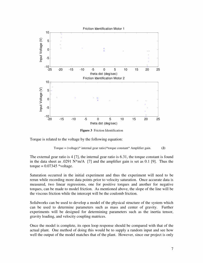
Verification Testing Procedures Motor Control Once the model is complete, its response should be compared with that of the actual plant. One method of doing this would be to supply a random input and see how well the output of the model matches that of the plant. However, since our project is only concerned with a step response, the verification process should only analyze any differences in the step response of the model and the plant. When verifying the model, non-linearities such as saturation, quantization, and friction modeling should be incorporated in the model. Launching System Testing on the repeatability of the launcher will be needed. This will be carried out by launching the ball several times using the same parameters. The air pressure will have to be measured to ensure a constant initial velocity. Also, to guarantee no leak in air pressure, a liquid will be sprayed on the surface of the launcher. If the liquid begins to bubble a pressure leak exists and needs to be sealed. Feedback System The first test is to find the relationship between the distance of the camera and the field of view. To achieve this, the camera was set up at different heights in increments of six inches. The camera was set to view a piece of masking tape five inches in length. The number of pixels in a row that contained the tape was measured. Since the resolution of the camera is known (288 by 352), the distance per pixel in inches can be found by the following formula: d/pixel= 1/(pixilated distance/5) (8) This can be used to find the total distance of the image. The angle of vision can be found by the formula: Θ=arcsin(d/(2h)) (9)

20

where d=total distance of image and h=height of the camera. The average Θ of for both the vertical and horizontal fields of view were found to be 0.26147 and 0.32176 radians respectively. The results are found in table 1 and 2.

Height (in) Y1 Y2

Pixelated Distance Pixels/inch inches/pixel inches/row theta

18 105 263 158 31.6 0.03164557 11.1392405 0.314587 24 132 249 117 23.4 0.042735043 15.042735 0.318761 30 147 240 93 18.6 0.053763441 18.9247312 0.320891 36 150 227 77 15.4 0.064935065 22.8571429 0.32305 42 152 217 65 13 0.076923077 27.0769231 0.328205 48 151 209 58 11.6 0.086206897 30.3448276 0.321607 54 178 229 51 10.2 0.098039216 34.5098039 0.325239

Table 1 Horizontal aperture angle

Height (in) X1 X2

Pixelated Distance Pixels/inch inches/pixel inches/row theta

18 29 183 154 30.8 0.032467532 9.35064935 0.262753 24 38 156 118 23.6 0.042372881 12.2033898 0.257059 30 53 147 94 18.8 0.053191489 15.3191489 0.258178 36 77 155 78 15.6 0.064102564 18.4615385 0.259306 42 93 158 65 13 0.076923077 22.1538462 0.266894 48 104 162 58 11.6 0.086206897 24.8275862 0.261594 54 118 169 51 10.2 0.098039216 28.2352941 0.264512

Table 2 Vertical aperture angle

From the aperture angles the field of view can be calculated by the equation:

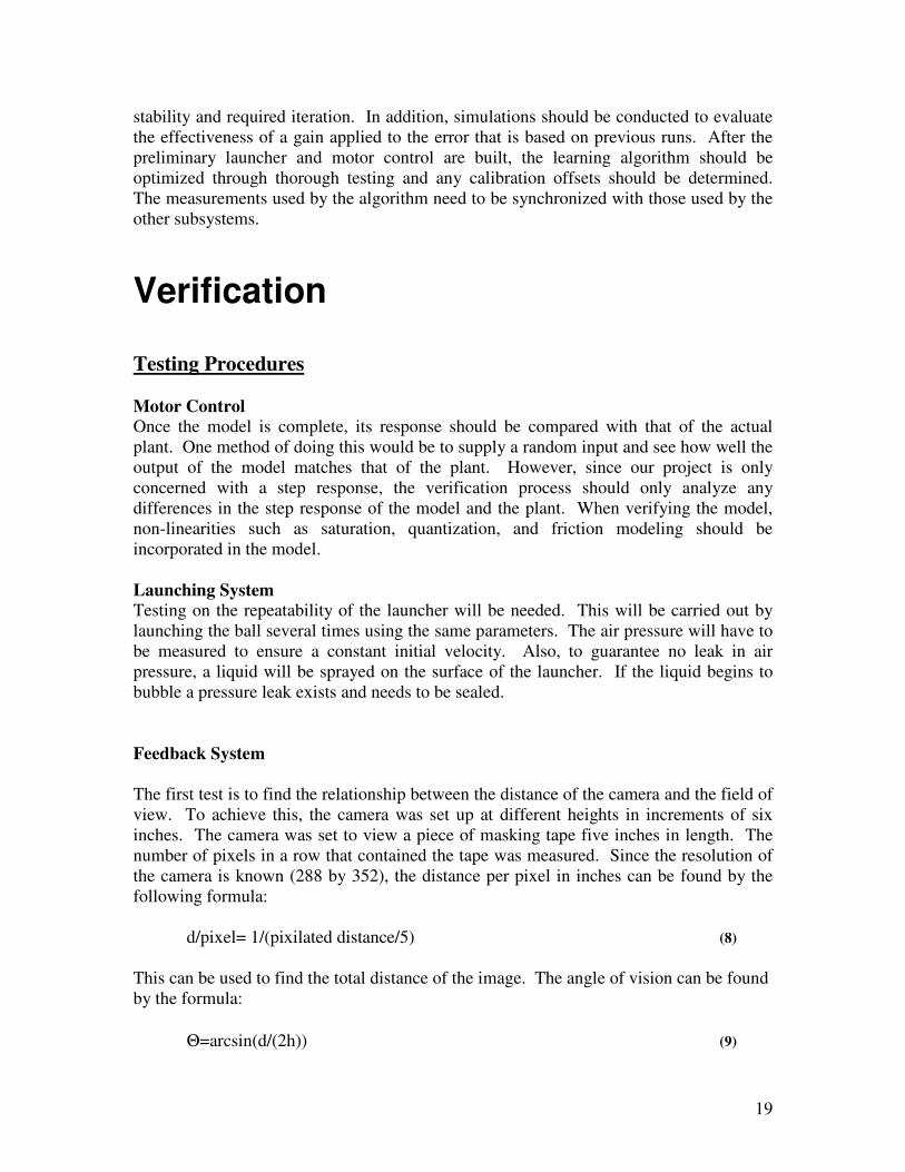
D=2*h*sin(Θ) (10) For the test setup the camera was set at 59 inches above the target. This gives a viewable area of 30.5 inches by 37.7 inches. The image of the test target is figure 14.

21

Figure 13 Test target

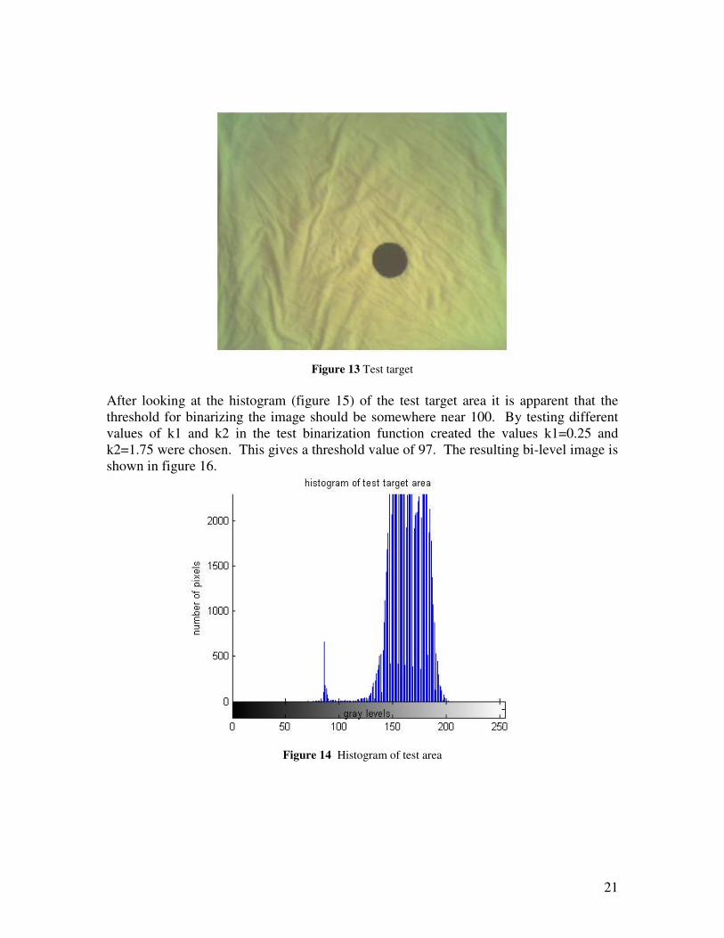
After looking at the histogram (figure 15) of the test target area it is apparent that the threshold for binarizing the image should be somewhere near 100. By testing different values of k1 and k2 in the test binarization function created the values k1=0.25 and k2=1.75 were chosen. This gives a threshold value of 97. The resulting bi-level image is shown in figure 16.

Figure 14 Histogram of test area

22

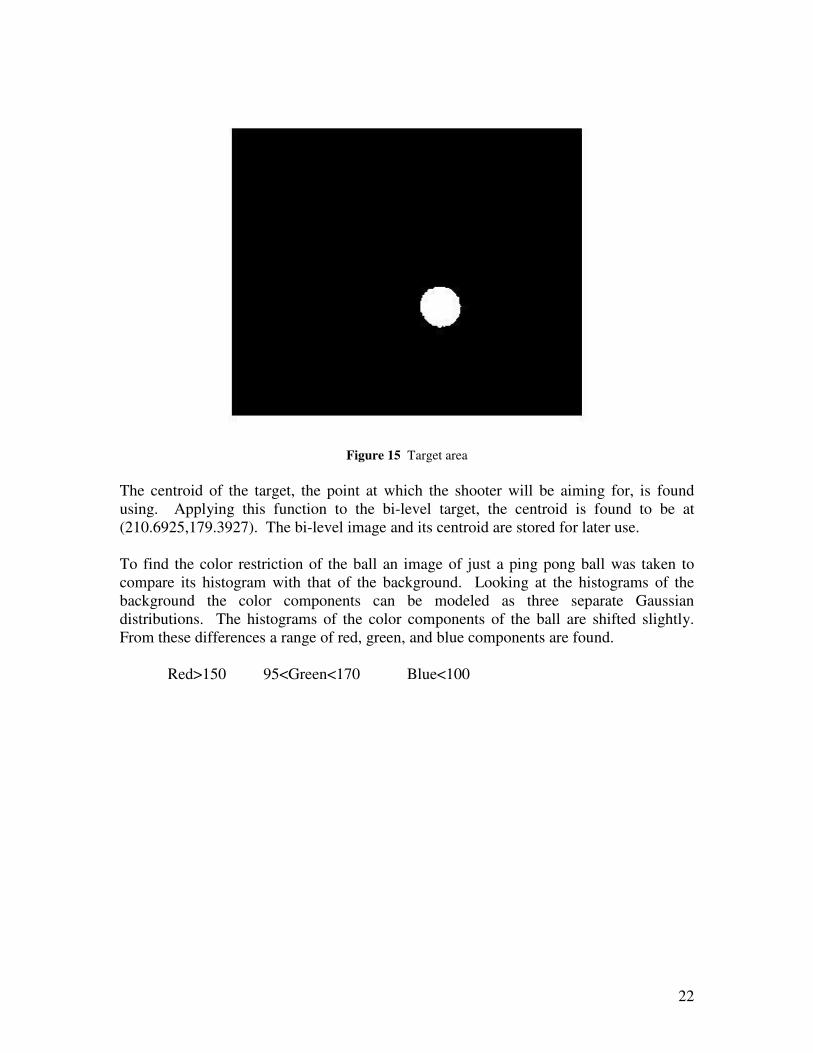
Figure 15 Target area

The centroid of the target, the point at which the shooter will be aiming for, is found using. Applying this function to the bi-level target, the centroid is found to be at (210.6925,179.3927). The bi-level image and its centroid are stored for later use. To find the color restriction of the ball an image of just a ping pong ball was taken to compare its histogram with that of the background. Looking at the histograms of the background the color components can be modeled as three separate Gaussian distributions. The histograms of the color components of the ball are shifted slightly. From these differences a range of red, green, and blue components are found. Red>150 95<Green<170 Blue<100

23

Figure 16 Color histograms of background

Figure 17 Color histograms of ball

Using those constraints, the image is binarized so that only the ball is shown. However it is quite noisy, so some morphological processing techniques are applied to reduce the noise, and the centroid is calculated.

24

Figure 18 Original image

Figure 19 Bi-level ball image before processing

25

Figure 20 Bi-level ball image after processing

The centroid of the ball is at (311.8665,208.2316), which is not in the range of the target. The file, distance.m, calculates the distance the shot is off by. In this case the shot was off by 101.1740 in the x direction and 28.8389 in the y direction. Learning Algorithm To verify the algorithm, a simulation using MATLAB/Simulink is developed based on the initial system model. The algorithm is tested against a physics model that determines the landing location of a projectile while simulating air drag (using constants Kz and Kr) and ball spin (using constant Kphi). This model can be seen in Appendix C. The script initially obtains pan and tilt angles based on projectile physics and the target location, then runs the simulation. If the target is missed by a magnitude of ‘r’ greater than .092 (diameter of the cup), or ‘�’ greater than .052 radians (angle of arc across the cup), the learning algorithm determines new pan and tilt algorithms and the physics model is simulated again using these new values. The algorithm was tested for several target locations using the drag and spin coefficients equal to 0.1. The target locations were kept within the ‘r’ dimension of 2.5m-1.5m, and ‘phi’ dimensions of -0.11 radians – 0.11 radians. This is due to the restrictions in field of view of the camera to be used for the image processing. It should be noted that the physics model was simulated using drag force and spin much larger than what would normally affect a table tennis ball in order to consider the worst case scenario. In each of the five target locations, the ball lands within the dimensions of the cup in three or less iterations. In the simulation however, the launcher is 100% repeatable, which will not be the case with the real launcher. Therefore it is expected that the algorithm will take much longer (up to eight shots) in order to reach the dimensions of the cup. The simulated trajectories can be seen in Appendix C.

26

When the algorithm is tested using the actual launcher and motor control, a manual feedback will be initially implemented using a measured grid over the target area. Tolerance Analysis The subsystem that affects the performance of the project the most is the launching system. The subsystem must have good repeatability in order to work well with the learning algorithm and the image processing. To ensure this, the pressure on the pneumatic valve must be consistent for every launch. In addition, the nozzle on the launch tube must be checked periodically to make sure that it has not worn out. The calibration of our system is another significant concern in the performance of the project. Since our system is divided into three separate physical parts (motor/launcher, camera, target area), it is necessary to adjust for the offsets between each part. This is especially important when interfacing between the image processing and the learning algorithm. Reference points shall be placed in the lab area to adjust the three parts in a consistent manner. The accuracy of the feedback system is another consideration. The camera uses discrete pixels and frames in order to represent the image. This will result in an inherent error between the actual location of the ball and the location determined by the image processing. This error can cause an unnecessary adjustment by the learning algorithm thus increasing the iterations required.

Cost and Schedule As time progresses dates will be shifted and group members reassigned as needed. However the current plan and due dates are listed below.

27

Table Project task list and resource allocation

Table Project Gantt Chart

The costs to design the Beirut Master 4000 are listed below. Items our cost commercial MATLAB 0 1900 Simulink 0 2800 MATLAB image acquisition toolbox 0 900 MATLAB image processing toolbox 0 900 XPC Target 0 4000

Table 3 Costs for computing

Items Our cost commercial

webcam 0 39.95 Piezo devices 12 12 pvc pipe and connections 20 20 Assorted resistors/op amps 0 20 Tubing 7.54 7.54 Electronic Valve 39.95 39.95

28

Table 4 Costs for feedback subsystem Items our cost commercial Ping Pong Ball Launcher 29.95 29.95 Pan motor 0 97.59 Tilt motor 0 97.59 pan/tilt gears 0 61.96 pan/tilt belts 0 7.92

Table 5 Costs for launching mechanism [1] Item our cost commercial labor (15 hours per week at $28 per hour) 0 25200 Total Cost 109.44 36134.45

Table 6 Labor and total cost of project

29

Bibliography 1. Andrews, Greg, Chris Colasuonno, and Aaron Hermann. “Ball on Plate Balancing System”. Internet. (2004) Available: http://www.cat.rpi.edu/~wen/ECSE4962S04/proposal/team2proposal.pdf, Feb. 2005. 2. Franklin, G.F., J.D. Powell, and A. Emami-Naeini, Feedback Control of Dynamic Systems, 4th Edition, Addison-Wesley, 2002. 3. Mi, Chris, Hui Lin, and Yi Zhang. “Iterative Learning Control of Antilock Braking in Electric and Hybrid Vehicles”. Internet. (2004) Available: http://www.ansoft.com/workshops/autoee04/mi.pdf, Feb. 2005. 4. Orr, Rusty. “UCB Physics Lecture Demonstrations”. Internet. (1997) Available: http://www.mip.berkeley.edu/physics/index.html, Feb. 2005. 5. Robert J. Schilling. Fundamentals of robotics, analysis and control. Prentice Hall, 1990. 6. SeGuine, Roy. “The Laws of Table Tennis”. Internet. (2004) Available: http://www.usatt.org, Feb. 2005. 7. Twarog, Chris, James Godlewski, Kevin Horbatt, and Paul Basantes. “Mr. Roizo Project Proposal – Computer Controlled Dancing Robot”. Internet. (2004) Available: http://www.cat.rpi.edu/~wen/ECSE4962S04/proposal/team4proposal.pdf, Feb. 2005. 8. Weisstein, Eric W. “Drag Coefficient”. Internet. (2005) Available: http://scienceworld.wolfram.com/physics/DragCoefficient.html, Feb. 2005. 9. Wen, John T. “ECSE 4460 Control System Design, Spring 2005”. Internet. (2005) Available: http://www.cat.rpi.edu/~wen/ECSE446S05/, Feb. 2005. 10. “Ball-Shooting Burp Gun”. Internet. (2005) Available: http://amos.shop.com/amos/cc/pcd/4614366/prd/6715663/ccsyn/260, Feb. 2005. 11. “DC Motor Specifications Sheet”. Internet. (2002) Available: http://www.pennmotion.com/pdf/lcg_bulletin.pdf, Feb. 2005. 12. “EM 027 Projectile Launcher”. Internet. (2002) Available: http://www.gunt.de/daten/04902700/datenblatt/04902700%202.pdf#search='projile%20launcher%20details', Feb. 2005.

30

13. “Projectile Launcher”. Internet. (2002) Available: http://www.science4schools.co.uk/acatalog/science4schools_Mechanics_12.html, Feb. 2005. 14. “Root-Finding”. Internet. (2004) Available: http://mathworld.wolfram.com/topics/Root-Finding.html, Feb. 2005. 15. “The Proportional Valve”. Internet. (2005) Available: http://www.clippard.com/store/byo_electronic/byo_proportional_valves.asp, Feb. 2005.

31

32

Appendix

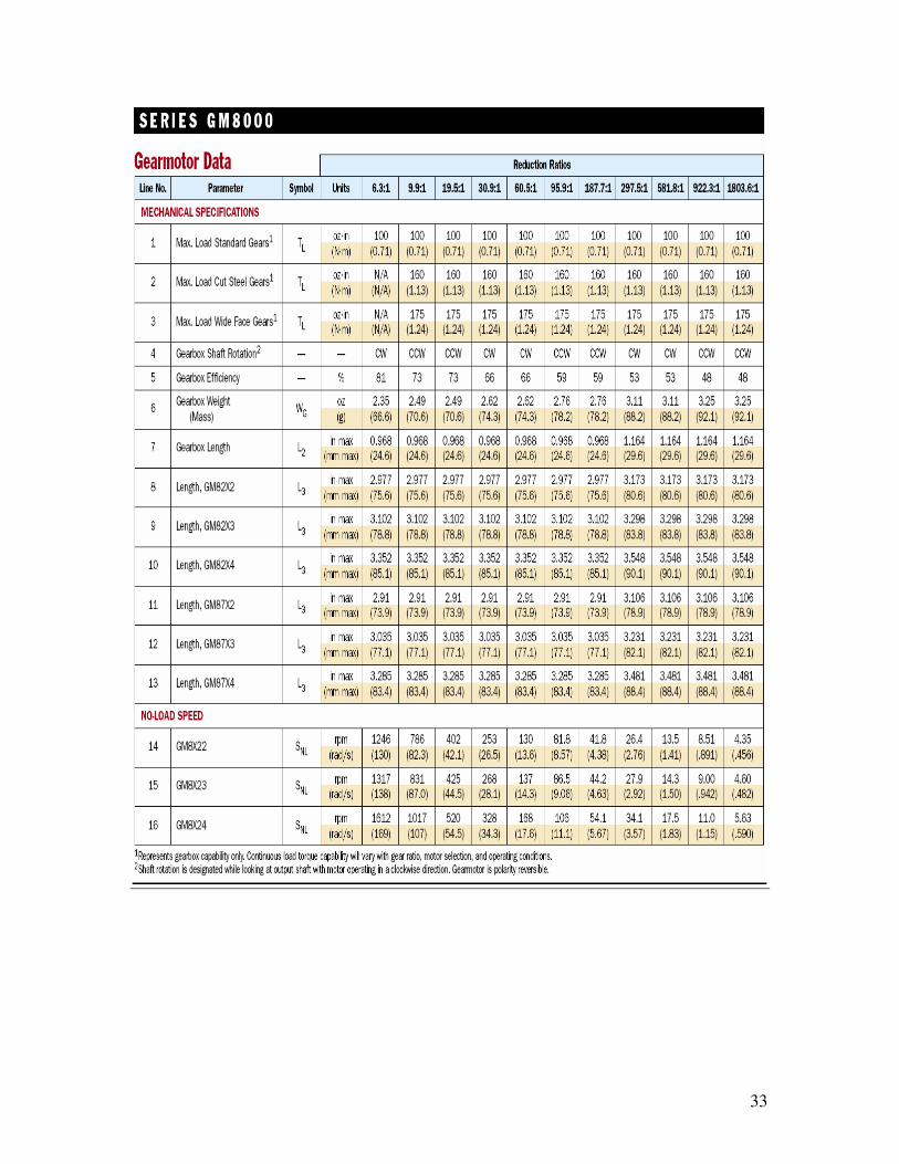
Appendix A: Specification Sheets for pan-and-tilt motors

33

34

35

36

Appendix B: CAD Drawings of system setup

37

Pan and Tilt model designed and built by Ben Potsaid. Launcher add-on built by Danish Zia.

38

Appendix C: Simulated trajectory paths with the learning algorithm This is the physics model used to calculate the following results.

-K-

dragx1

Kr

dragx

Kz

drag

sin

cos

finalphi

To Workspace5

finalr

To Workspace4

time

To Workspace3

phi

To Workspace2

r

To Workspace1

z

To Workspace

Switch1

SwitchSTOP

Stop Simulation

<

RelationalOperator

1s

1s

1s

1s

0

Constant9

0

Constant8

0

Constant7

h

Constant6

theta2

Constant5

theta1

Constant4

0

1

Constant2 0

Vo

Clock

-g

-g

Simulated results:

0 0.5 1 1.5 2 2.5-0.2

0

0.2

0.4

0.6

0.8

1

1.2

1.4

1.6

1.8

r

z

Kz = Kr = Kphi = 0.1, r(desired) = 2.5, phi(desired) = 0

shot 1shot 2shot 3

0.5

1

1.5

2

2.5

30

210

60

240

90

270

120

300

150

330

180 0

Kz = Kr = Kphi = 0.1, r(desired) = 2.5, phi(desired) = 0

shot 1shot 2shot 3

39

0 0.5 1 1.5 2 2.5-0.2

0

0.2

0.4

0.6

0.8

1

1.2

1.4

1.6

1.8

r

zKz = Kr = Kphi = 0.1, r(desired) = 2.25, phi(desired) = 0.06

shot 1shot 2

0.5

1

1.5

2

30

210

60

240

90

270

120

300

150

330

180 0

Kz = Kr = Kphi = 0.1, r(desired) = 2.25, phi(desired) = 0.06

shot 1shot 2

0 0.2 0.4 0.6 0.8 1 1.2 1.4 1.6 1.8 2-0.5

0

0.5

1

1.5

2

r

z

Kz = Kr = Kphi = 0.1, r(desired) = 2.0, phi(desired) = 0.11

shot 1shot 2

0.5

1

1.5

2

30

210

60

240

90

270

120

300

150

330

180 0

Kz = Kr = Kphi = 0.1, r(desired) = 2.0, phi(desired) = 0.11

shot 1shot 2

0 0.2 0.4 0.6 0.8 1 1.2 1.4 1.6 1.8-0.5

0

0.5

1

1.5

2Kz = Kr = Kphi = 0.1, r(desired) = 1.75, phi(desired) = -0.11

r

z

shot 1shot 2

0.5

1

1.5

30

210

60

240

90

270

120

300

150

330

180 0

Kz = Kr = Kphi = 0.1, r(desired) = 1.75, phi(desired) = -0.11

shot 1shot 2

40

0 0.5 1 1.5-0.5

0

0.5

1

1.5

2Kz = Kr = Kphi = 0.1, r(desired = 1.5), phi(desired) = -.06

r

zshot 1shot 2

0.5

1

1.5

30

210

60

240

90

270

120

300

150

330

180 0

Kz = Kr = Kphi = 0.1, r(desired = 1.5), phi(desired) = -.06

shot 1shot 2