Embed Size (px)
Citation preview
Machine Learning, 54, 5–32, 2004c© 2004 Kluwer Academic Publishers. Manufactured in The Netherlands.
Benchmarking Least Squares Support VectorMachine Classifiers
TONY VAN GESTEL [email protected] A.K. SUYKENS [email protected] of Electrical Engineering, ESAT/SISTA, Katholieke Universiteit Leuven, Belgium
BART BAESENS [email protected] VIAENE [email protected] VANTHIENEN [email protected] DEDENE [email protected] Institute for Research on Information Systems, Katholieke Universiteit Leuven, Belgium
BART DE MOOR [email protected] VANDEWALLE [email protected] of Electrical Engineering, ESAT/SISTA, Katholieke Universiteit Leuven, Belgium
Editor: Peter Bartlett
Abstract. In Support Vector Machines (SVMs), the solution of the classification problem is characterized bya (convex) quadratic programming (QP) problem. In a modified version of SVMs, called Least Squares SVMclassifiers (LS-SVMs), a least squares cost function is proposed so as to obtain a linear set of equations in thedual space. While the SVM classifier has a large margin interpretation, the LS-SVM formulation is related inthis paper to a ridge regression approach for classification with binary targets and to Fisher’s linear discriminantanalysis in the feature space. Multiclass categorization problems are represented by a set of binary classifiersusing different output coding schemes. While regularization is used to control the effective number of parametersof the LS-SVM classifier, the sparseness property of SVMs is lost due to the choice of the 2-norm. Sparse-ness can be imposed in a second stage by gradually pruning the support value spectrum and optimizing thehyperparameters during the sparse approximation procedure. In this paper, twenty public domain benchmarkdatasets are used to evaluate the test set performance of LS-SVM classifiers with linear, polynomial and ra-dial basis function (RBF) kernels. Both the SVM and LS-SVM classifier with RBF kernel in combination withstandard cross-validation procedures for hyperparameter selection achieve comparable test set performances.These SVM and LS-SVM performances are consistently very good when compared to a variety of methods de-scribed in the literature including decision tree based algorithms, statistical algorithms and instance based learningmethods. We show on ten UCI datasets that the LS-SVM sparse approximation procedure can be successfullyapplied.
Keywords: least squares support vector machines, multiclass support vector machines, sparse approximation
1. Introduction
Recently, Support Vector Machines (SVMs) have been introduced by Vapnik (Boser, Guyon,& Vapnik, 1992; Vapnik, 1995) for solving classification and nonlinear function estimation
6 T. VAN GESTEL ET AL.
problems (Cristianini & Shawe-Taylor, 2000; Scholkopf et al., 1997; Scholkopf, Burges,& Smola, 1998; Smola, Scholkopf, & Muller, 1998; Smola, 1999; Suykens & Vandewalle,1998; Vapnik, 1995, 1998a, 1998b). Within this new approach the training problem isreformulated and represented in such a way so as to obtain a (convex) quadratic programming(QP) problem. The solution to this QP problem is global and unique. In SVMs, it is possibleto choose several types of kernel functions including linear, polynomial, RBFs, MLPs withone hidden layer and splines, as long as the Mercer condition is satisfied. Furthermore,bounds on the generalization error are available from statistical learning theory (Cristianini& Shawe-Taylor, 2000; Smola, 1999; Vapnik, 1998a, 1998b), which are expressed in termsof the VC (Vapnik-Chervonenkis) dimension. An upper bound on this VC dimension canbe computed by solving another QP problem. Despite the nice properties of SVMs, thereare still a number of drawbacks concerning the selection of hyperparameters and the factthat the size of the matrix involved in the QP problem is directly proportional to the numberof training points.
A modified version of SVM classifiers, Least Squares SVMs (LS-SVMs) classifiers,was proposed in Suykens and Vandewalle (1999b). A two-norm was taken with equal-ity instead of inequality constraints so as to obtain a linear set of equations instead of aQP problem in the dual space. In this paper, it is shown that these modifications of theproblem formulation implicitly correspond to a ridge regression formulation with binarytargets ±1. In this sense, the LS-SVM formulation is related to regularization networks(Evgeniou, Pontil, & Poggio, 2001; Smola, Scholkopf, & Muller, 1998), Gaussian Pro-cesses regression (Williams, 1998) and to the ridge regression type of SVMs for nonlinearfunction estimation (Saunders, Gammerman, & Vovk, 1998; Smola, 1999), but with theinclusion of a bias term which has implications towards algorithms. The primal-dual for-mulations of the SVM framework and the equality constraints of the LS-SVM formulationallow to make extensions towards recurrent neural networks (Suykens & Vandewalle, 2000)and nonlinear optimal control (Suykens, Vandewalle, & De Moor, 2001). In this paper, theadditional insight of the linear decision line in the feature space is used to relate the im-plicit LS-SVM regression approach to a regularized form of Fisher’s discriminant analysis(Bishop, 1995; Duda & Hart, 1973; Fisher, 1936) in the feature space (Baudat & Anouar,2000; Mika et al., 1999). By applying the Mercer condition, this so-called Kernel FisherDiscriminant is obtained as the solution to a generalized eigenvalue problem (Baudat &Anouar, 2000; Mika et al., 1999).
The QP-problem of the corresponding SVM formulation is typically solved by Inte-rior Point (IP) methods (Cristianini & Shawe-Taylor, 2000; Smola, 1999), SequentialMinimal Optimization (SMO) (Platt, 1998) and iteratively reweighted least squares ap-proaches (IRWLS) (Navia-Vazquez et al., 2001), while LS-SVMs (Suykens & Vandewalle,1999b; Suykens et al., 2002; Van Gestel et al., 2001, 2002; Viaene et al., 2001) result intoa set of linear equations. Efficient iterative methods for solving large scale linear systemsare available in numerical linear algebra (Golub & Van Loan, 1989). In Suykens et al.(1999) a conjugate gradient based iterative method has been developed for solving the re-lated Karush-Kuhn-Tucker system. In this paper, the algorithm is further refined in orderto combine it with hyperparameter selection. A drawback of LS-SVMs is that sparsenessis lost due the choice of a 2-norm. However, this can be circumvented in a second stage
BENCHMARKING LS-SVM CLASSIFIERS 7
by a pruning procedure which is based upon removing training points guided by the sortedsupport value spectrum and does not involve the computation of inverse Hessian matricesas in classical neural network pruning methods (Suykens et al., 2002). This is importantin view of an equivalence between sparse approximation and SVMs as shown in Girosi(1998).
A straightforward extension of LS-SVMs to multiclass problems has been proposed inSuykens and Vandewalle (1999c), where additional outputs are taken in order to encodemulticlasses as is often done in classical neural networks methodology (Bishop, 1995).This approach is different from standard multiclass SVM approaches. In Suykens andVandewalle (1999c) the multi two-spiral benchmark problem, which is known to be hardfor classical neural networks, was solved with an LS-SVM with a minimal number of bitsin the class coding and yielded an excellent generalization performance. This approach isfurther extended here to different types of output codings for the classes, like one-versus-all,error correcting and one-versus-one codes.
In this paper, we report the performance of LS-SVMs on twenty public domain bench-mark datasets (Blake & Merz, 1998). Ten binary and ten multiclass classification problemswere considered. On each dataset linear, polynomial and RBF (Radial Basis Function)kernels were trained and tested. The performances of the simple minimum output cod-ing and advanced one-versus-one coding are also compared on the multiclass problems.The LS-SVM hyperparameters were determined from a 10-fold cross-validation proce-dure by grid search in the hyperparameter space. The LS-SVM generalization ability wasestimated on independent test sets in all of the cases and results of additional random-izations on all datasets are reported. In the experimental setup two third of the data wasused to construct the classifier and one third was reserved for out-of-sample testing. Af-ter optimization of the hyperparameters, a very good test set performance is achievedby LS-SVMs on all twenty datasets. At this point comparisons on the same randomizeddatasets have been made with reference classifiers including the SVM classifier, decisiontree based algorithms, statistical algorithms and instance based learning methods (Aha &Kibler, 1991; Breiman et al., 1984; Duda & Hart, 1973; Holte, 1993; John & Langley,1995; Lim, Loh, & Shih, 2000; Ripley, 1996; Witten & Frank, 2000). In most cases SVMsand LS-SVMs with RBF kernel perform at least as good as SVM and LS-SVMs withlinear kernel which means that often additional insight can be obtained whether the opti-mal decision boundary is strongly nonlinear or not. Furthermore, we successfully confirmthe LS-SVM sparse approximation procedure that has been proposed in Suykens et al.(2002) on 10 UCI benchmark datasets with optimal hyperparameter determination duringpruning.
This paper is organized as follows. In Section 2, we review the basic LS-SVM formulationfor binary classification and relate the LS-SVM formulation to Kernel Fisher DiscriminantAnalysis. The multiclass categorization problem is reformulated as a set of binary classifica-tion problems in Section 3. The sparse approximation procedure is discussed in Section 4. Aconjugate gradient algorithm for large scale applications is discussed in Section 5. Section 6elaborates on the selection of the hyperparameters with 10-fold cross-validation. Section 7presents the empirical findings of LS-SVM classifiers achieved on 20 UCI benchmarkdatasets in comparison with other methods.
8 T. VAN GESTEL ET AL.
2. LS-SVMs for binary classification
Given a training set {(xi , yi )}Ni=1 with input data xi ∈ IRn and corresponding binary class la-
bels yi ∈ {−1, +1}, the SVM classifier, according to Vapnik’s original formulation(Boser, Guyon, & Vapnik, 1992; Cristianini & Shawe-Taylor, 2000; Scholkopf et al.,1997; Scholkopf, Burges, & Smola, 1998; Smola, Scholkopf, & Muller, 1998; Vapnik,1995, 1998a, 1998b), satisfies the following conditions:
{wT ϕ(xi ) + b ≥ +1, if yi = +1
wT ϕ(xi ) + b ≤ −1, if yi = −1(1)
which is equivalent to
yi [wT ϕ(xi ) + b] ≥ 1, i = 1, . . . , N . (2)
The nonlinear function ϕ(·): Rn → R
nh maps the input space to a high (and possibly infinite)dimensional feature space. In primal weight space the classifier then takes the form
y(x) = sign[wT ϕ(x) + b], (3)
but, on the other hand, is never evaluated in this form. One defines the optimization problem:
minw,b,ξ
J (w, ξ ) = 1
2wT w + C
N∑i=1
ξi (4)
subject to
{yi [wT ϕ(xi ) + b] ≥ 1 − ξi , i = 1, . . . , N
ξi ≥ 0, i = 1, . . . , N .(5)
The variables ξi are slack variables that are needed in order to allow misclassifications inthe set of inequalities (e.g., due to overlapping distributions). The positive real constantC should be considered as a tuning parameter in the algorithm. For nonlinear SVMs, theQP-problem and the classifier are never solved and evaluated in this form. Instead a dualspace formulation and representation is obtained by applying the Mercer condition (seeCristianini & Shawe-Taylor, 2000; Scholkopf et al., 1997; Scholkopf, Burges, & Smola,1998; Smola, 1999; Vapnik, 1995, 1998a, 1998b) for details.
Vapnik’s SVM classifier formulation was modified in Suykens and Vandewalle (1999b)into the following LS-SVM formulation:
minw,b,e
J (w, e) = 1
2wT w + γ
1
2
N∑i=1
e2i (6)
BENCHMARKING LS-SVM CLASSIFIERS 9
subject to the equality constraints
yi [wT ϕ(xi ) + b] = 1 − ei , i = 1, . . . , N . (7)
This formulation consists of equality instead of inequality constraints and takes into accounta squared error with regularization term similar to ridge regression.
The solution is obtained after constructing the Lagrangian:
L(w, b, e; α) = J (w, b, e) −N∑
i=1
αi {yi [wT ϕ(xi ) + b] − 1 + ei }, (8)
where αi ∈ IR are the Lagrange multipliers that can be positive or negative in the LS-SVM formulation. From the conditions for optimality, one obtains the Karush-Kuhn-Tucker(KKT) system:
∂L∂w
= 0 → w =N∑
i=1
αi yiϕ(xi )
∂L∂b
= 0 →N∑
i=1
αi yi = 0
∂L∂ei
= 0 → αi = γ ei , i = 1, . . . , N
∂L∂αi
= 0 → yi [wT ϕ(xi ) + b] − 1 + ei = 0, i = 1, . . . , N .
(9)
Note that sparseness is lost which is clear from the condition αi = γ ei . As in standardSVMs, we never calculate w nor ϕ(xi ). Therefore, we eliminate w and e yielding (Suykens& Vandewalle, 1999b)
[0 yT
y � + γ −1 I
] [b
α
]=
[0
1v
](10)
with y = [y1, . . . , yN ], 1v = [1, . . . , 1], e = [e1, . . . , eN ], α = [α1, . . . , αN ]. Mercer’scondition is applied within the � matrix
�i j = yi y j ϕ(xi )T ϕ(x j ) = yi y j K (xi , x j ). (11)
For the kernel function K (·, ·) one typically has the following choices:
K (x, xi ) = xTi x, (linear kernel)
K (x, xi ) = (1 + xT
i x/
c)d
, (polynomial kernel of degree d)
K (x, xi ) = exp{−∥∥x − xi
∥∥22
/σ 2
}, (RBF kernel)
K (x, xi ) = tanh(κ xT
i x + θ), (MLP kernel),
10 T. VAN GESTEL ET AL.
where d , c, σ , κ and θ are constants. Notice that the Mercer condition holds for all c, σ ∈ IR+
and d ∈ N values in the polynomial and RBF case, but not for all possible choices of κ
and θ in the MLP case. The scale parameters c, σ and κ determine the scaling of the inputsin the polynomial, RBF and MLP kernel function. This scaling is related to the bandwidthof the kernel in statistics, where it is shown that the bandwidth is an important parameterof the generalization behavior of a kernel method (Rao, 1983). The LS-SVM classifier isthen constructed as follows:
y(x) = sign
[N∑
i=1
αi yi K (x, xi ) + b
]. (12)
A simple and practical way to construct binary MLP classifiers is to use a regressionformulation (Bishop, 1995; Duda & Hart, 1973), where one uses the targets ±1 to encode thefirst and second class, respectively. By the use of equality constraints with targets {−1, +1},the LS-SVM formulation (6)–(7) implicitly corresponds to a regression formulation withregularization (Bishop, 1995; Duda & Hart, 1973; Saunders, Gammerman, & Vovk, 1998;Suykens & Vandewalle, 1999b). Indeed, by multiplying the error ei with yi ∈ {−1, +1},the error term ED = ∑N
i=1 e2i becomes
ED = 1
2
N∑i=1
e2i = 1
2
N∑i=1
(yi ei )2 = 1
2
N∑i=1
(yi − (wT ϕ(xi ) + b))2. (13)
Neglecting the bias term in the LS-SVM formulation, this regression interpretation relatesthe LS-SVM classifier formulation to regularization networks (Evgeniou, Pontil, & Poggio,2001; Smola, Scholkopf, & Muller, 1998), Gaussian Processes regression (Williams, 1998)and to the ridge regression type of SVMs for nonlinear function estimation (Saunders,Gammerman, & Vovk, 1998; Smola, 1999). SVMs and LS-SVMs give the additional insightof the kernel-induced feature space, while the same expressions are obtained in the dualspace as with regularization networks for function approximation and Gaussian Processeson the first level of the evidence framework (MacKay, 1995; Van Gestel et al., 2002).
Given this regression interpretation, the bias term in the LS-SVM formulation allows toexplicitly relate the LS-SVM classifier to regularized Fisher’s linear discriminant analysisin the feature space (ridge regression) (Friedman, 1989). Fisher’s linear discriminant isdefined as the linear function with maximum ratio of between-class scatter to within-classscatter (Bishop, 1995; Duda & Hart, 1973; Fisher, 1936). By defining N+ and N− as thenumber of training data of class +1 and −1, respectively, Fisher’s linear discriminant (inthe feature space) with regularization is obtained by minimizing
minwF ,bF
1
2wT
FwF + γF
2
N∑i=1
(ti − wT
Fϕ(xi ) + bF
)2, (14)
with appropriate targets ti = −(N/N−) if yi = −1 and ti = N/N+ if yi = +1 (Fisher,1936).
BENCHMARKING LS-SVM CLASSIFIERS 11
This least squares regression problem (Bishop, 1995; Duda & Hart, 1973) yields the samelinear discriminant wF as is obtained from a generalized eigenvalue problem in Baudatand Anouar (2000) and Mika et al. (1999), where the bias term is determined by, e.g.,cross-validation. The regression formulation (14) with Fisher’s targets {−N/N−, +N/N+}chooses the bias term bF based on the sample mean (Bishop, 1995; Duda & Hart, 1973),while the targets {−1, +1} correspond to an asymptotically optimal least squares ap-proximation of Bayes’ discriminant for two Gaussian distributions (Duda & Hart, 1973).The difference between the LS-SVM classifier and the regularized Fisher discriminant isthat the corresponding regression interpretations use different targets being {−1, +1} and{−N/N−, +N/N+}, respectively. It can be proven that for γF = γ , the relation betweenthe two classifier formulations is given 2wF = w and 2bF = b − 1
N
∑Ni=1 yi . Hence, by
solving the linear set of Eq. (10) in the dual space for the LS-SVM classifier, e.g., by alarge scale algorithm (Golub & Van Loan, 1989; Suykens et al., 1999), the regularizedFisher discriminant is also obtained. Both choices for the targets will be compared in theexperimental setup, where the Fisher discriminant is denoted by LS-SVMF (LS-SVM withFisher’s discriminant targets).
3. Multiclass LS-SVMs
Multiclass categorization problems are typically solved by reformulating the multiclassproblem with M classes into a set of L binary classification problems (Allwein, Schapire, &Singer, 2000; Bishop, 1995; Ripley, 1996; Utschik, 1998). To each class Cm , m = 1, . . . , M ,a unique codeword cm = [y(1)
m , y(2)m , . . . , y(L)
m ] = y(1:L)m ∈ {−1, 0, +1}L is assigned, where
each binary classifier fl(x), l = 1, . . . , L , discriminates between the corresponding outputbit yl . The use of 0 in the codeword is explained below.
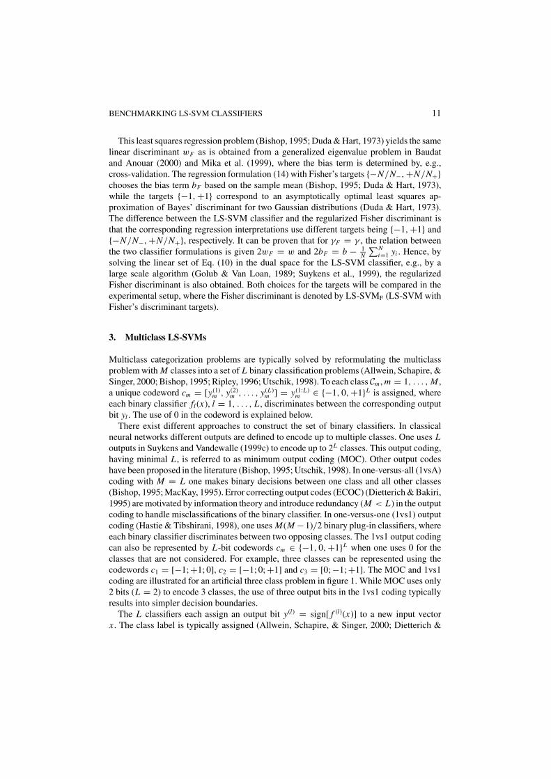
There exist different approaches to construct the set of binary classifiers. In classicalneural networks different outputs are defined to encode up to multiple classes. One uses Loutputs in Suykens and Vandewalle (1999c) to encode up to 2L classes. This output coding,having minimal L , is referred to as minimum output coding (MOC). Other output codeshave been proposed in the literature (Bishop, 1995; Utschik, 1998). In one-versus-all (1vsA)coding with M = L one makes binary decisions between one class and all other classes(Bishop, 1995; MacKay, 1995). Error correcting output codes (ECOC) (Dietterich & Bakiri,1995) are motivated by information theory and introduce redundancy (M < L) in the outputcoding to handle misclassifications of the binary classifier. In one-versus-one (1vs1) outputcoding (Hastie & Tibshirani, 1998), one uses M(M −1)/2 binary plug-in classifiers, whereeach binary classifier discriminates between two opposing classes. The 1vs1 output codingcan also be represented by L-bit codewords cm ∈ {−1, 0, +1}L when one uses 0 for theclasses that are not considered. For example, three classes can be represented using thecodewords c1 = [−1; +1; 0], c2 = [−1; 0; +1] and c3 = [0; −1; +1]. The MOC and 1vs1coding are illustrated for an artificial three class problem in figure 1. While MOC uses only2 bits (L = 2) to encode 3 classes, the use of three output bits in the 1vs1 coding typicallyresults into simpler decision boundaries.
The L classifiers each assign an output bit y(l) = sign[ f (l)(x)] to a new input vectorx . The class label is typically assigned (Allwein, Schapire, & Singer, 2000; Dietterich &
12 T. VAN GESTEL ET AL.
−2.5 −2 −1.5 −1 −0.5 0 0.5 1 1.5 2 2.5−2.5
−2
−1.5
−1
−0.5
0
0.5
1
1.5
2
2.5
−2.5 −2 −1.5 −1 −0.5 0 0.5 1 1.5 2 2.5−2.5
−2
−1.5
−1
−0.5
0
0.5
1
1.5
2
2.5
Figure 1. Importance of output coding on the shape of the binary decision lines illustrated on an artificial threeclass problem (◦, � and �) with Gaussian distributions having equal covariance matrices. The shape of the binarydecision lines depends on the representation of the multiclass problem problem as a set of binary classificationproblems. Left: minimal output coding (MOC) using 2 bits and assuming equal class distributions, the first binaryclassifier discriminates between (�, �) and◦, while the second discriminates between � and (�,◦). Right: one-versus-one output (1vs1) coding using three bits, the three binary classifiers discriminate between �, �; �,◦ and�,◦, respectively. The use of MOC results into nonlinear decision lines, while linear decision lines are obtainedwith the 1vs1 coding.
Bakiri, 1995; Sejnowski & Rosenberg, 1987) to the corresponding output code with minimalHamming distance H (y(1:L), cm), with
H(y(1:L), cm
) =L∑
l=1
0 if y(l) = y(l)m and y(l) �= 0 and y(l)
m �= 01
2if y(l) = 0 or y(l)
m = 0
1 if y(l) �= y(l)m and y(l) �= 0 and y(l)
m �= 0.
When one considers the 1vs1 output coding scheme as a voting between each pair of classes,it is easy to see that the codeword with minimal Hamming distance corresponds to the classwith the maximal number of votes.
In this paper, we restrict ourselves to the use of minimum output coding (MOC) (Suykens& Vandewalle, 1999c) and one versus one (1vs1) coding (Hastie & Tibshirani, 1998). Eachbinary classifier f (l)(x), l = 1, . . . , L , is inferred on the training set D(l) = {(xi , y(l)
i ) | i =1, . . . , N and y(l)
i ∈ {−1, +1}}, consisting of N (l) ≤ N training points, by solving
[0 y(l)T
y(l) �(l) + γ (l)−1I
] [b(l)
α(l)
]=
[01v
](15)
where �i j,l = Kl(xi , x j ). The binary classifier fl(x) is then obtained as f (l)(x) =sign[
∑N (l)
i=1 y(l)i α
(l)i K (l)(x, xi ) + b(l)].
Since the binary classifiers f (l)(x) are trained and designed independently, the superscript(l) will be omitted in the next Sections in order to simplify the notation.
BENCHMARKING LS-SVM CLASSIFIERS 13
4. Sparse approximation using LS-SVMs
As mentioned before, a drawback of LS-SVMs in comparison with standard QP type SVMsis that sparseness is lost due to the choice of the 2-norm in (6), which is also clear from thefact that αi = γ ei in (9). For standard SVMs one typically has that many αi values are exactlyequal to zero. In Suykens et al. (2002), it was shown how sparseness can be imposed to LS-SVMs by a pruning procedure which is based upon the sorted support value spectrum. This isimportant considering the equivalence between SVMs and sparse approximation, shown inGirosi (1998). Indeed, the αi values obtained from the linear system (10) reveal the relativeimportance of the training data points with respect to each other. This information is thenemployed to remove less important points from the training set, where the omitted data pointscorrespond to zero αi values. An important difference with pruning methods in classicalneural networks (Bishop, 1995; Hassibi & Stork, 1993; Le Cun, Denker, & Solla, 1990), e.g.,optimal brain damage and optimal brain surgeon, is that in the LS-SVM pruning procedureno inverse of a Hessian matrix has to be computed. The LS-SVM pruning procedure canalso be related to Interior Point and IRWLS methods for SVMs (Navia-Vazquez et al.,2001; Smola, 1999), where a linear system of the same form as (10) is solved in eachiteration step until the conditions for optimality and the resulting sparseness property ofthe SVM are obtained. In each step of the IRWLS solution the whole training set is stilltaken into account and the sparse SVM solution is obtained after convergence. The LS-SVMpruning procedure removes a certain percentage of training data points in each iteration step.The pruning of large positive and small negative αi values results into support vectors thatare located far from and near to the decision boundary. An LS-SVM pruning procedure inwhich only the support values near the decision boundary with large αi does yield a poorergeneralization behavior, which can be intuitively understood since the LS-SVMs in the laststeps are trained only on a specific part of the global training set. In this sense, the sparseLS-SVM is somewhat in between the SVM solution with support vectors near the decisionboundary and the relevance vector machine (Tipping, 2001) with support vectors far fromthe decision boundary. When one assumes that the variance of the noise is not constantor when the dataset may contain outliers, one can also use a weighted least squares costfunction (Suykens et al., 2002; Van Gestel et al., 2001, 2002). In this case sparseness is alsointroduced by putting the weights in the cost function to zero for data points with large errors.
Hence, by plotting the spectrum of the sorted |αi | values of the binary LS-SVM, one canevaluate which data points are most significant for contributing to the LS-SVM classifier(12). Sparseness is imposed in a second stage by gradually omitting the least important datafrom the training set using a pruning procedure (Suykens et al., 2002): in each pruning stepall data points of which the absolute value of the support value is smaller than a threshold areremoved. The height of the threshold is chosen such that in each step, e.g., 5% of the totalnumber of training points are removed. The LS-SVM is then re-estimated on the reducedtraining set and the pruning procedure is repeated until a user-defined performance indexstarts decreasing. The pruning procedure consists of the following steps:
1. Train LS-SVM based on N points.2. For each output, remove a small amount of points (e.g., 5% of the set) with smallest
values in the sorted |αi | spectra.
14 T. VAN GESTEL ET AL.
3. Re-train the LS-SVM based on the reduced training set (Suykens & Vandewalle, 1999b).In order to increase a user-defined performance index and to be able to prune more, onecan refine the hyper- and kernel parameters.
4. Go to 2, unless the user-defined performance index degrades significantly. A one-tailedpaired t-test can be used, e.g., in combination with 10-fold cross-validation to reportsignificant decreases in the average validation performance.
For the multiclass case, this pruning procedure is applied to each binary classifier f (l)(x),l = 1, . . . , L .
5. Implementation
In this section, an iterative implementation is discussed for solving the linear system (10).Efficient iterative algorithms, such as Krylov subspace and Conjugate Gradient (CG) meth-ods, exists in numerical linear algebra (Golub & Van Loan, 1989) to solve a linear sys-tem Ax = B with positive definite matrix A = AT > 0. Considering the cost functionV (x) = 1
2 xTAx − xTB, the solution of the corresponding linear system is also found asarg minx V (x). In the Hestenes-Stiefel conjugate gradient algorithm (Golub & Van Loan,1989), one starts from an initial guess x0 and V (xi ) is decreased in each iteration step i asfollows:
i = 0; x = x0; r = B − Axi ; ρ0 = ‖r‖22
while (i < imax) ∧ (√
ρi > ε1||B||2) ∧ (V (xi−1) − V (xi ) > ε2),i = i + 1if i = 1
p = relse
βi = ρi−1/ρi−2
p = r + βi pendifv = Apαi = ρi−1/(pT v)x = x + αi
r = r − αiv
ρi = ‖r‖22
V (xi ) = − 12 xT
i (r + B)endwhile
For A ∈ IRN×N and B ∈ IRN , the algorithm requires one matrix-vector multiplicationv = Ap and 10N flops, while only four vectors of length N are stored: x, r, p and v. ForA = I +C ≥ 0 and rank(C) = rc, the algorithm converges in at most rc +1 steps, assuminginfinite machine precision. However, the rate of convergence may be much higher, dependingon the condition number of A. The algorithm stops when one of the three stopping criteriais satisfied. While the first criterion stops the algorithm after maximal imax iteration steps,
BENCHMARKING LS-SVM CLASSIFIERS 15
the second criterion is based on the norm of the residuals. The third criterion is based on theevolution of the cost function V (x), which is evaluated as V (x) = 1
2 xT (Ax −B)− 12 xTB =
− 12 xT (r + B). The constants imax, ε1 and ε2 are determined by the user, e.g., according to
the required numerical accuracy. The use of iterative algorithms to solve large scale linearsystems is preferred over the use of direct methods, since direct methods would involve acomputational complexity of O(N 3) and memory requirements of O(N 2) (Golub & VanLoan, 1989), while the computational complexity of the CG algorithm is at most O(rc N 2)when A is stored. As the number of iterations i is typically smaller than rc, an additionalreduction in the computational requirements is obtained. When the matrix A is too large forthe memory requirements, one can recompute A in each iteration step, which costs O(N 2)operations per step but also reduces the memory requirements to O(N ).
In order to apply the CG algorithm to (10), the system matrix A involved in the set oflinear equations should be positive definite. Therefore, according to Suykens et al. (1999)the system (10) is transformed into
[s 0
0 H
] [b
α + H−1Y b
]=
[−0 + yT H−11v
1v
](16)
with s = Y T H−1Y > 0 and H = H T = � + γ −1 IN > 0. The system (10) is now solvedas follows (Suykens et al., 1999):
1. Use the CG algorithm to solve η, ν from
Hη = y (17)
Hν = 1v. (18)
2. Compute s = yT η.3. Find solution: b = ηT 1v/s and α = ν − ηb .
When no information on the solution x is available, one typically chooses x0 = 0 forsolving (17) and (18). In the next section, the initial guess will be used to speed up thecalculations when solving (10) for different choices of the hyperparameter γ . For a newγnew value, the initial guess for η and ν can be based on the assumption that the training seterrors ei,new do not significantly differ from the errors ei,old, i = 1, . . . , N corresponding tothe previous choice γold (Smola, 1999). Hence we can write in vector notation enew eold
or αnew γnew/γoldαold, while the bias term is not changed bnew bold. From (17) and(18) in step 1 and from the solutions for α and b in steps 2 and 3, it can be seen thatthese initial guesses for αnew and bnew are obtained by choosing ηnew,0 = γnew/γoldηold
and νnew,0 = γnew/γoldνold. Krylov subspace methods also allow to solve the linear systemsimultaneously for different regularization parameters γ .
For large N , the matrix A = H = � + γ −1 IN with dimensions N × N cannot be storeddue to memory limitations, the elementsAi j have to be re-calculated in each iteration. SinceA is symmetric, this requires N (N − 1)/2 kernel function evaluations. Since A is equal in(17) and (18), the number of kernel function evaluations is reduced by a factor 1/2 when
16 T. VAN GESTEL ET AL.
simultaneously solving (17) and (18) for η and ν. Also observe that the condition numberincreases when γ is increased or when less weight is put onto the regularization term. Weused at most imax = 150 iterations and put the other constants to ε1 = ε2 = 10−9, which isgiving good results on all tried datasets.
6. Hyperparameter selection
Different techniques exist for tuning the hyperparameters related to the regularization con-stant and the parameter of the kernel function. Among the available tuning methods we findminimization of the VC-dimension (Bishop, 1995; Smola, 1999; Suykens & Vandewalle,1999a; Vapnik, 1998, 1998a), the use of cross-validation methods, bootstrapping techniques,Bayesian inference (Bishop, 1995; Kwok, 2000; MacKay, 1995; Van Gestel et al., 2001,2002), etc. In this section, the regularization and kernel parameters of each binary classifierare selected using a simple 10-fold cross-validation procedure.
In the case of an RBF kernel, the hyperparameter γ , the kernel parameter σ and the testset performance of the binary LS-SVM classifier are estimated using the following steps:
1. Set aside 2/3 of the data for the training/validation set and the remaining 1/3 for testing.2. Starting from i = 0, perform 10-fold cross-validation on the training/validation data for
each (σ, γ ) combination from the initial candidate tuning sets �0 = {0.5, 5, 10, 15, 25,
50, 100, 250, 500} · √n and �0 = {0.01, 0.05, 0.1, 0.5, 1, 5, 10, 50, 100, 500, 1000}.
3. Choose optimal (σ, γ ) from the tuning sets �i and �i by looking at the best cross-validation performance for each (σ, γ ) combination.
4. If i = imax, go to step 5; else i := i + 1, construct a locally refined grid �i × �i aroundthe optimal hyperparameters (σ, γ ) and go to step 3.
5. Construct the LS-SVM classifier using the total training/validation set for the optimalchoice of the tuned hyperparameters (σ, γ ).
6. Assess the test set accuracy by means of the independent test set.
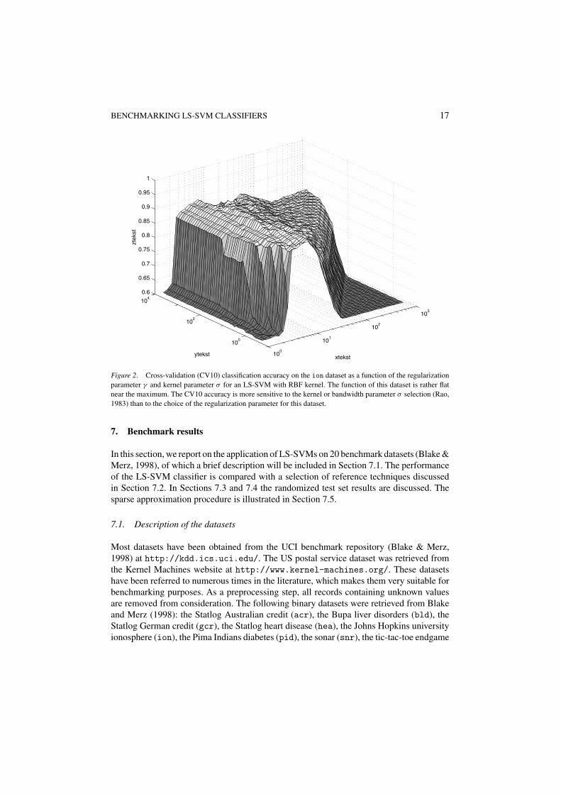
In this benchmarking study, imax was typically chosen to imax = 3 using 3 additionalrefine searches. This involves a fine-tuned selection of the σ and γ parameters. It shouldbe remarked that the refining of the grid is not always necessary as the 10-fold (CV10)cross-validation performance typically has a flat maximum, as can be seen from figure 2.
In combination with the iterative algorithm of Section 5, one solves the linear systems(17) and (18) for the first grid point starting from initial value x0 = 0. For the next γ value inthe grid, the solutions η and ν were initialized accordingly. When changing σ , we initializedν and η with the corresponding solutions related to the previous σ value. Depending on thedistance between the points in the grid, the average reduction of the number of iterationsteps amounts to 10%–50% with respect to starting from x0 = 0 for all (σ, γ ) combinations.
For the polynomial kernel functions the hyperparameters γ and c were tuned by a similarprocedure, while the regularization parameter γ of the linear kernel was selected from arefined set � based upon the cross-validation performance. For multiclass problems, thecross-validation procedure is repeated for each binary classifier f (l)(x), l = 1, . . . , L .
BENCHMARKING LS-SVM CLASSIFIERS 17
100
101
102
103
100
102
104
0.6
0.65
0.7
0.75
0.8
0.85
0.9
0.95
1
xtekstytekst
ztek
st
Figure 2. Cross-validation (CV10) classification accuracy on the ion dataset as a function of the regularizationparameter γ and kernel parameter σ for an LS-SVM with RBF kernel. The function of this dataset is rather flatnear the maximum. The CV10 accuracy is more sensitive to the kernel or bandwidth parameter σ selection (Rao,1983) than to the choice of the regularization parameter for this dataset.
7. Benchmark results
In this section, we report on the application of LS-SVMs on 20 benchmark datasets (Blake &Merz, 1998), of which a brief description will be included in Section 7.1. The performanceof the LS-SVM classifier is compared with a selection of reference techniques discussedin Section 7.2. In Sections 7.3 and 7.4 the randomized test set results are discussed. Thesparse approximation procedure is illustrated in Section 7.5.
7.1. Description of the datasets
Most datasets have been obtained from the UCI benchmark repository (Blake & Merz,1998) at http://kdd.ics.uci.edu/. The US postal service dataset was retrieved fromthe Kernel Machines website at http://www.kernel-machines.org/. These datasetshave been referred to numerous times in the literature, which makes them very suitable forbenchmarking purposes. As a preprocessing step, all records containing unknown valuesare removed from consideration. The following binary datasets were retrieved from Blakeand Merz (1998): the Statlog Australian credit (acr), the Bupa liver disorders (bld), theStatlog German credit (gcr), the Statlog heart disease (hea), the Johns Hopkins universityionosphere (ion), the Pima Indians diabetes (pid), the sonar (snr), the tic-tac-toe endgame
18 T. VAN GESTEL ET AL.
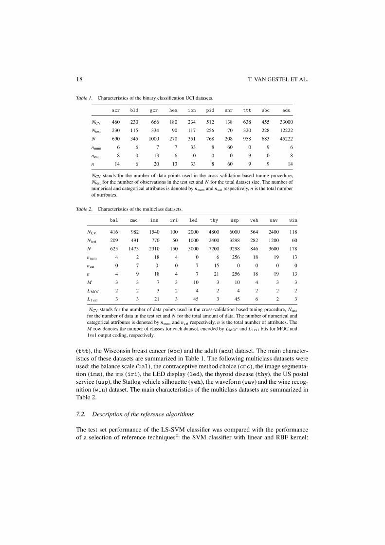
Table 1. Characteristics of the binary classification UCI datasets.
acr bld gcr hea ion pid snr ttt wbc adu
NCV 460 230 666 180 234 512 138 638 455 33000
Ntest 230 115 334 90 117 256 70 320 228 12222
N 690 345 1000 270 351 768 208 958 683 45222
nnum 6 6 7 7 33 8 60 0 9 6
ncat 8 0 13 6 0 0 0 9 0 8
n 14 6 20 13 33 8 60 9 9 14
NCV stands for the number of data points used in the cross-validation based tuning procedure,Ntest for the number of observations in the test set and N for the total dataset size. The number ofnumerical and categorical attributes is denoted by nnum and ncat respectively, n is the total numberof attributes.
Table 2. Characteristics of the multiclass datasets.
bal cmc ims iri led thy usp veh wav win
NCV 416 982 1540 100 2000 4800 6000 564 2400 118
Ntest 209 491 770 50 1000 2400 3298 282 1200 60
N 625 1473 2310 150 3000 7200 9298 846 3600 178
nnum 4 2 18 4 0 6 256 18 19 13
ncat 0 7 0 0 7 15 0 0 0 0
n 4 9 18 4 7 21 256 18 19 13
M 3 3 7 3 10 3 10 4 3 3
LMOC 2 2 3 2 4 2 4 2 2 2
L1vs1 3 3 21 3 45 3 45 6 2 3
NCV stands for the number of data points used in the cross-validation based tuning procedure, Ntest
for the number of data in the test set and N for the total amount of data. The number of numerical andcategorical attributes is denoted by nnum and ncat respectively, n is the total number of attributes. TheM row denotes the number of classes for each dataset, encoded by LMOC and L1vs1 bits for MOC and1vs1 output coding, respectively.
(ttt), the Wisconsin breast cancer (wbc) and the adult (adu) dataset. The main character-istics of these datasets are summarized in Table 1. The following multiclass datasets wereused: the balance scale (bal), the contraceptive method choice (cmc), the image segmenta-tion (ims), the iris (iri), the LED display (led), the thyroid disease (thy), the US postalservice (usp), the Statlog vehicle silhouette (veh), the waveform (wav) and the wine recog-nition (win) dataset. The main characteristics of the multiclass datasets are summarized inTable 2.
7.2. Description of the reference algorithms
The test set performance of the LS-SVM classifier was compared with the performanceof a selection of reference techniques2: the SVM classifier with linear and RBF kernel;
BENCHMARKING LS-SVM CLASSIFIERS 19
the decision tree algorithm C4.5 (Quinlan, 1993), Holte’s one-rule classifier (oneR) (Holte,1993); statistical algorithms like linear discriminant analysis (LDA), quadratic discriminantanalysis (QDA), logistic regression (logit) (Bishop, 1995; Duda & Hart, 1973; Ripley, 1996);instance based learners (IB) (Aha & Kibler, 1991) and Naive Bayes (John & Langley, 1995).The oneR, LDA, QDA, logit, NBk and NBn require no parameter tuning. For C4.5, we usedthe default confidence level of 25% for pruning, which is the value that is commonly usedin the machine learning literature. We also experimented with other pruning levels on someof the datasets, but found no significant performance increases. For IB we used both 1(IB1) and 10 (IB10) nearest neighbours. We used both standard Naive Bayes with thenormal approximation (NBn) (Duda & Hart, 1973) and the kernel approximation (NBk) fornumerical attributes (John & Langley, 1995). The default classifier or majority rule (Maj.Rule) was included as a baseline in the comparison tables. All comparisons were made onthe same randomizations. For another comparison study among 22 decision tree, 9 statisticaland 2 neural network algorithms, we refer to (Lim, Loh, & Shih, 2000).
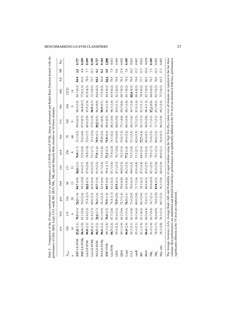
The comparison is performed on an out-of-sample test set consisting of 1/3 of the data.The first 2/3 of the randomized data was reserved for training and/or cross-validation. Foreach algorithm, we report the average test set performance and sample standard deviationon 10 randomizations in each domain (Bay, 1999; De Groot, 1986; Domingos, 1996; Lim,Loh, & Shih, 2000). The best average test set performance was underlined and denoted inbold face for each domain. Performances that are not significantly different at the 5% levelfrom the top performance with respect to a one-tailed paired t-test are tabulated in boldface. Statistically significant underperformances at the 1% level are emphasized. Perfor-mances significantly different at the 5% level but not a the 1% level are reported in nor-mal script. Since the observations on the randomizations are not independent (Dietterich,1998), we remark that this standard t-test is used only as a (common) heuristic to indi-cate statistical difference between average accuracies on the ten randomizations. Ranks areassigned to each algorithm starting from 1 for the best average performance and endingwith 18 and 28 for the algorithm with worst performance, for the binary and multiclassdomains, respectively. Averaging over all domains, the Average Accuracy (AA) and Av-erage Rank (AR) are reported for each algorithm (Lim, Loh, & Shih, 2000). A Wilcoxonsigned rank test of equality of medians is used on both AA and AR to check whether theperformance of an algorithm is significantly different from the algorithm with the highestaccuracy. A Probability of a Sign Test (PST) is also reported comparing each algorithmto the algorithm with best accuracy. The results of these significance tests on the averagedomain performances are denoted in the same way as the performances on each individualdomain.
7.3. Performance of the binary LS-SVM classifier
In this subsection, we present and discuss the results obtained by applying the empiricalsetup, outlined in Section 6, on the 10 UCI binary benchmark datasets described above. Allexperiments were carried out on Sun Ultra5 Workstations and on Pentium II and III PCs.For the kernel types, we used RBF kernels, linear (Lin) and polynomial (Pol) kernels (withdegree d = 2, . . . , 10). Both the performance of LS-SVM targets {−1, +1} and Regularized
20 T. VAN GESTEL ET AL.
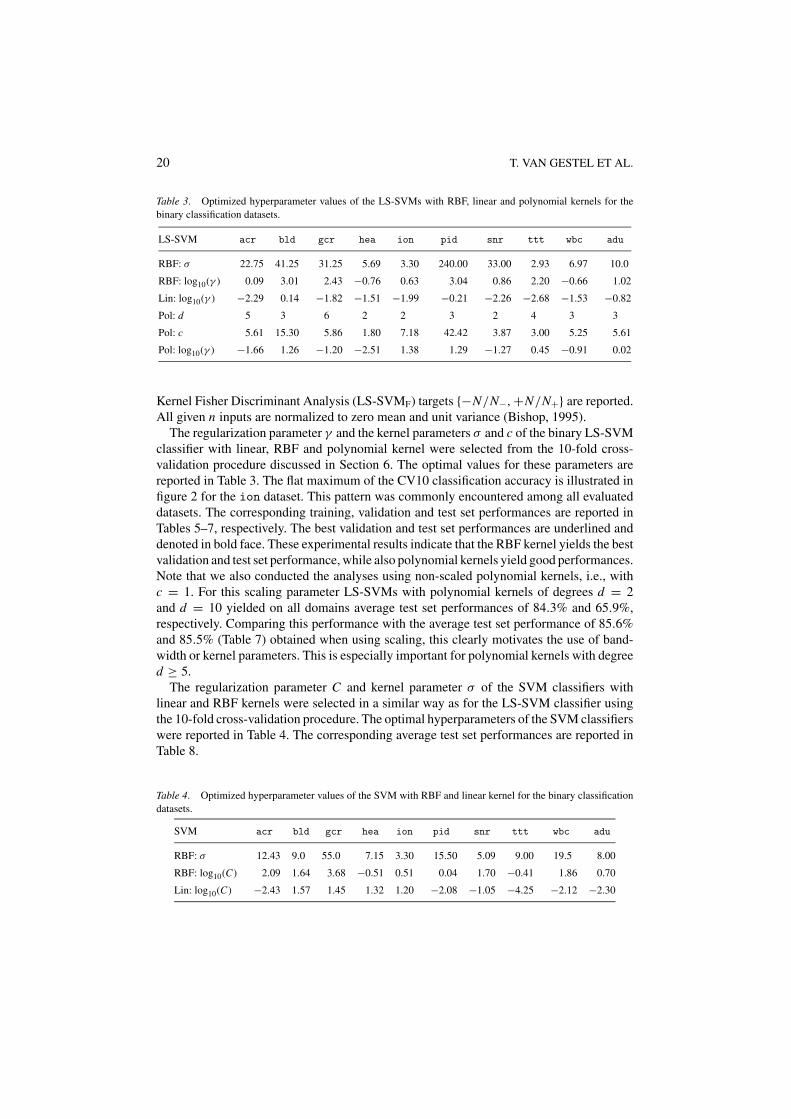
Table 3. Optimized hyperparameter values of the LS-SVMs with RBF, linear and polynomial kernels for thebinary classification datasets.
LS-SVM acr bld gcr hea ion pid snr ttt wbc adu
RBF: σ 22.75 41.25 31.25 5.69 3.30 240.00 33.00 2.93 6.97 10.0
RBF: log10(γ ) 0.09 3.01 2.43 −0.76 0.63 3.04 0.86 2.20 −0.66 1.02
Lin: log10(γ ) −2.29 0.14 −1.82 −1.51 −1.99 −0.21 −2.26 −2.68 −1.53 −0.82
Pol: d 5 3 6 2 2 3 2 4 3 3
Pol: c 5.61 15.30 5.86 1.80 7.18 42.42 3.87 3.00 5.25 5.61
Pol: log10(γ ) −1.66 1.26 −1.20 −2.51 1.38 1.29 −1.27 0.45 −0.91 0.02
Kernel Fisher Discriminant Analysis (LS-SVMF) targets {−N/N−, +N/N+} are reported.All given n inputs are normalized to zero mean and unit variance (Bishop, 1995).
The regularization parameter γ and the kernel parameters σ and c of the binary LS-SVMclassifier with linear, RBF and polynomial kernel were selected from the 10-fold cross-validation procedure discussed in Section 6. The optimal values for these parameters arereported in Table 3. The flat maximum of the CV10 classification accuracy is illustrated infigure 2 for the ion dataset. This pattern was commonly encountered among all evaluateddatasets. The corresponding training, validation and test set performances are reported inTables 5–7, respectively. The best validation and test set performances are underlined anddenoted in bold face. These experimental results indicate that the RBF kernel yields the bestvalidation and test set performance, while also polynomial kernels yield good performances.Note that we also conducted the analyses using non-scaled polynomial kernels, i.e., withc = 1. For this scaling parameter LS-SVMs with polynomial kernels of degrees d = 2and d = 10 yielded on all domains average test set performances of 84.3% and 65.9%,respectively. Comparing this performance with the average test set performance of 85.6%and 85.5% (Table 7) obtained when using scaling, this clearly motivates the use of band-width or kernel parameters. This is especially important for polynomial kernels with degreed ≥ 5.
The regularization parameter C and kernel parameter σ of the SVM classifiers withlinear and RBF kernels were selected in a similar way as for the LS-SVM classifier usingthe 10-fold cross-validation procedure. The optimal hyperparameters of the SVM classifierswere reported in Table 4. The corresponding average test set performances are reported inTable 8.
Table 4. Optimized hyperparameter values of the SVM with RBF and linear kernel for the binary classificationdatasets.
SVM acr bld gcr hea ion pid snr ttt wbc adu
RBF: σ 12.43 9.0 55.0 7.15 3.30 15.50 5.09 9.00 19.5 8.00
RBF: log10(C) 2.09 1.64 3.68 −0.51 0.51 0.04 1.70 −0.41 1.86 0.70
Lin: log10(C) −2.43 1.57 1.45 1.32 1.20 −2.08 −1.05 −4.25 −2.12 −2.30
BENCHMARKING LS-SVM CLASSIFIERS 21
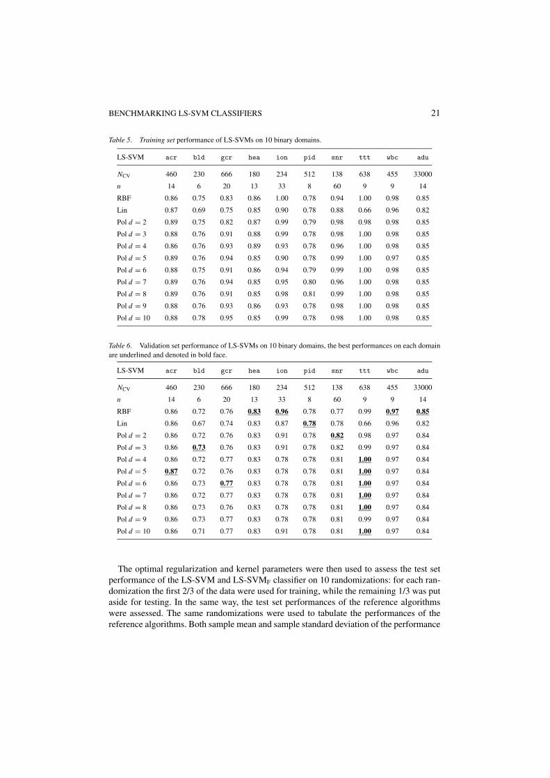
Table 5. Training set performance of LS-SVMs on 10 binary domains.
LS-SVM acr bld gcr hea ion pid snr ttt wbc adu
NCV 460 230 666 180 234 512 138 638 455 33000
n 14 6 20 13 33 8 60 9 9 14
RBF 0.86 0.75 0.83 0.86 1.00 0.78 0.94 1.00 0.98 0.85
Lin 0.87 0.69 0.75 0.85 0.90 0.78 0.88 0.66 0.96 0.82
Pol d = 2 0.89 0.75 0.82 0.87 0.99 0.79 0.98 0.98 0.98 0.85
Pol d = 3 0.88 0.76 0.91 0.88 0.99 0.78 0.98 1.00 0.98 0.85
Pol d = 4 0.86 0.76 0.93 0.89 0.93 0.78 0.96 1.00 0.98 0.85
Pol d = 5 0.89 0.76 0.94 0.85 0.90 0.78 0.99 1.00 0.97 0.85
Pol d = 6 0.88 0.75 0.91 0.86 0.94 0.79 0.99 1.00 0.98 0.85
Pol d = 7 0.89 0.76 0.94 0.85 0.95 0.80 0.96 1.00 0.98 0.85
Pol d = 8 0.89 0.76 0.91 0.85 0.98 0.81 0.99 1.00 0.98 0.85
Pol d = 9 0.88 0.76 0.93 0.86 0.93 0.78 0.98 1.00 0.98 0.85
Pol d = 10 0.88 0.78 0.95 0.85 0.99 0.78 0.98 1.00 0.98 0.85
Table 6. Validation set performance of LS-SVMs on 10 binary domains, the best performances on each domainare underlined and denoted in bold face.
LS-SVM acr bld gcr hea ion pid snr ttt wbc adu
NCV 460 230 666 180 234 512 138 638 455 33000
n 14 6 20 13 33 8 60 9 9 14
RBF 0.86 0.72 0.76 0.83 0.96 0.78 0.77 0.99 0.97 0.85
Lin 0.86 0.67 0.74 0.83 0.87 0.78 0.78 0.66 0.96 0.82
Pol d = 2 0.86 0.72 0.76 0.83 0.91 0.78 0.82 0.98 0.97 0.84
Pol d = 3 0.86 0.73 0.76 0.83 0.91 0.78 0.82 0.99 0.97 0.84
Pol d = 4 0.86 0.72 0.77 0.83 0.78 0.78 0.81 1.00 0.97 0.84
Pol d = 5 0.87 0.72 0.76 0.83 0.78 0.78 0.81 1.00 0.97 0.84
Pol d = 6 0.86 0.73 0.77 0.83 0.78 0.78 0.81 1.00 0.97 0.84
Pol d = 7 0.86 0.72 0.77 0.83 0.78 0.78 0.81 1.00 0.97 0.84
Pol d = 8 0.86 0.73 0.76 0.83 0.78 0.78 0.81 1.00 0.97 0.84
Pol d = 9 0.86 0.73 0.77 0.83 0.78 0.78 0.81 0.99 0.97 0.84
Pol d = 10 0.86 0.71 0.77 0.83 0.91 0.78 0.81 1.00 0.97 0.84
The optimal regularization and kernel parameters were then used to assess the test setperformance of the LS-SVM and LS-SVMF classifier on 10 randomizations: for each ran-domization the first 2/3 of the data were used for training, while the remaining 1/3 was putaside for testing. In the same way, the test set performances of the reference algorithmswere assessed. The same randomizations were used to tabulate the performances of thereference algorithms. Both sample mean and sample standard deviation of the performance
22 T. VAN GESTEL ET AL.
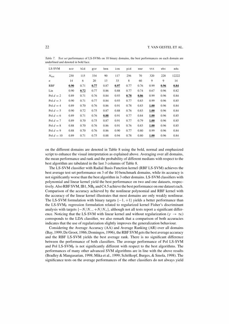
Table 7. Test set performance of LS-SVMs on 10 binary domains, the best performances on each domain areunderlined and denoted in bold face.
LS-SVM acr bld gcr hea ion pid snr ttt wbc adu
Ntest 230 115 334 90 117 256 70 320 228 12222
n 14 6 20 13 33 8 60 9 9 14
RBF 0.90 0.71 0.77 0.87 0.97 0.77 0.76 0.99 0.96 0.84
Lin 0.90 0.72 0.77 0.86 0.88 0.77 0.74 0.67 0.96 0.82
Pol d = 2 0.89 0.71 0.76 0.84 0.93 0.78 0.86 0.99 0.96 0.84
Pol d = 3 0.90 0.71 0.77 0.84 0.93 0.77 0.83 0.99 0.96 0.85
Pol d = 4 0.89 0.70 0.76 0.86 0.91 0.78 0.83 1.00 0.96 0.84
Pol d = 5 0.90 0.72 0.75 0.87 0.88 0.76 0.83 1.00 0.96 0.84
Pol d = 6 0.89 0.71 0.76 0.88 0.91 0.77 0.84 1.00 0.96 0.85
Pol d = 7 0.89 0.70 0.75 0.87 0.91 0.77 0.79 1.00 0.96 0.85
Pol d = 8 0.88 0.70 0.76 0.86 0.91 0.76 0.83 1.00 0.96 0.85
Pol d = 9 0.88 0.70 0.76 0.86 0.90 0.77 0.80 0.99 0.96 0.84
Pol d = 10 0.89 0.71 0.75 0.88 0.94 0.78 0.80 1.00 0.96 0.84
on the different domains are denoted in Table 8 using the bold, normal and emphasizedscript to enhance the visual interpretation as explained above. Averaging over all domains,the mean performance and rank and the probability of different medians with respect to thebest algorithm are tabulated in the last 3 columns of Table 8.
The LS-SVM classifier with Radial Basis Function kernel (RBF LS-SVM) achieves thebest average test set performance on 3 of the 10 benchmark domains, while its accuracy isnot significantly worse than the best algorithm in 3 other domains. LS-SVM classifiers withpolynomial and linear kernel yield the best performance on two and one datasets, respec-tively. Also RBF SVM, IB1, NBk and C4.5 achieve the best performance on one dataset each.Comparison of the accuracy achieved by the nonlinear polynomial and RBF kernel withthe accuracy of the linear kernel illustrates that most domains are only weakly nonlinear.The LS-SVM formulation with binary targets {−1, +1} yields a better performance thanthe LS-SVMF regression formulation related to regularized kernel Fisher’s discriminantanalysis with targets {−N/N−, +N/N+}, although not all tests report a significant differ-ence. Noticing that the LS-SVM with linear kernel and without regularization (γ → ∞)corresponds to the LDA classifier, we also remark that a comparison of both accuraciesindicates that the use of regularization slightly improves the generalization behaviour.
Considering the Average Accuracy (AA) and Average Ranking (AR) over all domains(Bay, 1999; De Groot, 1986; Domingos, 1996), the RBF SVM gets the best average accuracyand the RBF LS-SVM yields the best average rank. There is no significant differencebetween the performance of both classifiers. The average performance of Pol LS-SVMand Pol LS-SVMF is not significantly different with respect to the best algorithms. Theperformances of many other advanced SVM algorithms are in line with the above results(Bradley & Mangasarian, 1998; Mika et al., 1999; Scholkopf, Burges, & Smola, 1998). Thesignificance tests on the average performances of the other classifiers do not always yield
BENCHMARKING LS-SVM CLASSIFIERS 23Ta
ble
8.C
ompa
riso
nof
the
10tim
esra
ndom
ized
test
set
perf
orm
ance
ofL
S-SV
Man
dL
S-SV
MF
(lin
ear,
poly
nom
ial
and
Rad
ial
Bas
isFu
nctio
nke
rnel
)w
ithth
epe
rfor
man
ceof
LD
A,Q
DA
,Log
it,C
4.5,
oneR
,IB
1,IB
10,N
Bk,N
Bn
and
the
Maj
ority
Rul
ecl
assi
fier
on10
bina
rydo
mai
ns.
acr
bld
gcr
hea
ion
pid
snr
ttt
wbc
adu
AA
AR
P ST
Nte
st23
011
533
490
117
256
7032
022
812
222
n14
620
1333
860
99
14
RB
FL
S-SV
M87
.0(2
.1)
70.2
(4.1
)76
.3(1
.4)
84.7
(4.8
)96
.0(2
.1)
76.8
(1.7
)73
.1(4
.2)
99.0
(0.3
)96
.4(1
.0)
84.7
(0.3
)84
.43.
50.
727
RB
FL
S-SV
MF
86.4
(1.9
)65
.1(2
.9)
70.8
(2.4
)83
.2(5
.0)
93.4
(2.7
)72
.9(2
.0)
73.6
(4.6
)97
.9(0
.7)
96.8
(0.7
)77
.6(1
.3)
81.8
8.8
0.10
9
Lin
LS-
SVM
86.8
(2.2
)65
.6(3
.2)
75.4
(2.3
)84
.9(4
.5)
87.9
(2.0
)76
.8(1
.8)
72.6
(3.7
)66
.8(3
.9)
95.8
(1.0
)81
.8(0
.3)
79.4
7.7
0.10
9
Lin
LS-
SVM
F86
.5(2
.1)
61.8
(3.3
)68
.6(2
.3)
82.8
(4.4
)85
.0(3
.5)
73.1
(1.7
)73
.3(3
.4)
57.6
(1.9
)96
.9(0
.7)
71.3
(0.3
)75
.712
.10.
109
PolL
S-SV
M86
.5(2
.2)
70.4
(3.7
)76
.3(1
.4)
83.7
(3.9
)91
.0(2
.5)
77.0
(1.8
)76
.9(4
.7)
99.5
(0.5
)96
.4(0
.9)
84.6
(0.3
)84
.24.
10.
727
PolL
S-SV
MF
86.6
(2.2
)65
.3(2
.9)
70.3
(2.3
)82
.4(4
.6)
91.7
(2.6
)73
.0(1
.8)
77.3
(2.6
)98
.1(0
.8)
96.9
(0.7
)77
.9(0
.2)
82.0
8.2
0.34
4
RB
FSV
M86
.3(1
.8)
70.4
(3.2
)75
.9(1
.4)
84.7
(4.8
)95
.4(1
.7)
77.3
(2.2
)75
.0(6
.6)
98.6
(0.5
)96
.4(1
.0)
84.4
(0.3
)84
.44.
01.
000
Lin
SVM
86.7
(2.4
)67
.7(2
.6)
75.4
(1.7
)83
.2(4
.2)
87.1
(3.4
)77
.0(2
.4)
74.1
(4.2
)66
.2(3
.6)
96.3
(1.0
)83
.9(0
.2)
79.8
7.5
0.02
1
LD
A85
.9(2
.2)
65.4
(3.2
)75
.9(2
.0)
83.9
(4.3
)87
.1(2
.3)
76.7
(2.0
)67
.9(4
.9)
68.0
(3.0
)95
.6(1
.1)
82.2
(0.3
)78
.99.
60.
004
QD
A80
.1(1
.9)
62.2
(3.6
)72
.5(1
.4)
78.4
(4.0
)90
.6(2
.2)
74.2
(3.3
)53
.6(7
.4)
75.1
(4.0
)94
.5(0
.6)
80.7
(0.3
)76
.212
.60.
002
Log
it86
.8(2
.4)
66.3
(3.1
)76
.3(2
.1)
82.9
(4.0
)86
.2(3
.5)
77.2
(1.8
)68
.4(5
.2)
68.3
(2.9
)96
.1(1
.0)
83.7
(0.2
)79
.27.
80.
109
C4.
585
.5(2
.1)
63.1
(3.8
)71
.4(2
.0)
78.0
(4.2
)90
.6(2
.2)
73.5
(3.0
)72
.1(2
.5)
84.2
(1.6
)94
.7(1
.0)
85.6
(0.3
)79
.910
.20.
021
oneR
85.4
(2.1
)56
.3(4
.4)
66.0
(3.0
)71
.7(3
.6)
83.6
(4.8
)71
.3(2
.7)
62.6
(5.5
)70
.7(1
.5)
91.8
(1.4
)80
.4(0
.3)
74.0
15.5
0.00
2
IB1
81.1
(1.9
)61
.3(6
.2)
69.3
(2.6
)74
.3(4
.2)
87.2
(2.8
)69
.6(2
.4)
77.7
(4.4
)82
.3(3
.3)
95.3
(1.1
)78
.9(0
.2)
77.7
12.5
0.02
1
IB10
86.4
(1.3
)60
.5(4
.4)
72.6
(1.7
)80
.0(4
.3)
85.9
(2.5
)73
.6(2
.4)
69.4
(4.3
)94
.8(2
.0)
96.4
(1.2
)82
.7(0
.3)
80.2
10.4
0.03
9
NB
k81
.4(1
.9)
63.7
(4.5
)74
.7(2
.1)
83.9
(4.5
)92
.1(2
.5)
75.5
(1.7
)71
.6(3
.5)
71.7
(3.1
)97
.1(0
.9)
84.8
(0.2
)79
.77.
30.
109
NB
n76
.9(1
.7)
56.0
(6.9
)74
.6(2
.8)
83.8
(4.5
)82
.8(3
.8)
75.1
(2.1
)66
.6(3
.2)
71.7
(3.1
)95
.5(0
.5)
82.7
(0.2
)76
.612
.30.
002
Maj
.rul
e56
.2(2
.0)
56.5
(3.1
)69
.7(2
.3)
56.3
(3.8
)64
.4(2
.9)
66.8
(2.1
)54
.4(4
.7)
66.2
(3.6
)66
.2(2
.4)
75.3
(0.3
)63
.217
.10.
002
The
Ave
rage
Acc
urac
y(A
A),
Ave
rage
Ran
k(A
R)
and
Prob
abili
tyof
equa
lm
edia
nsus
ing
the
Sign
Test
(PST
)ta
ken
over
all
dom
ains
are
repo
rted
inth
ela
stth
ree
colu
mns
.Bes
tper
form
ance
sar
eun
derl
ined
and
deno
ted
inbo
ldfa
ce,p
erfo
rman
ces
nots
igni
fican
tlydi
ffer
enta
tthe
5%le
vela
rede
note
din
bold
face
,per
form
ance
ssi
gnifi
cant
lydi
ffer
enta
tthe
1%le
vela
reem
phas
ized
.
24 T. VAN GESTEL ET AL.
the same results. Generally speaking, the performance of Lin LS-SVM, Lin SVM, Logit andNBk is not significantly different at the 1% level. Also the performances of LS-SVMs withFisher’s discriminant targets (LS-SVMF) are not signifantly different at the 1%. Generallyspeaking, the results of Table 8 allow to conclude that the SVM and LS-SVM formulationsachieve very good test set performances compared to the other reference algorithms.
7.4. Performance of the multiclass LS-SVM classifier
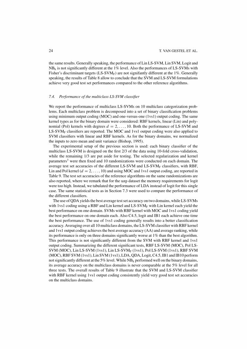
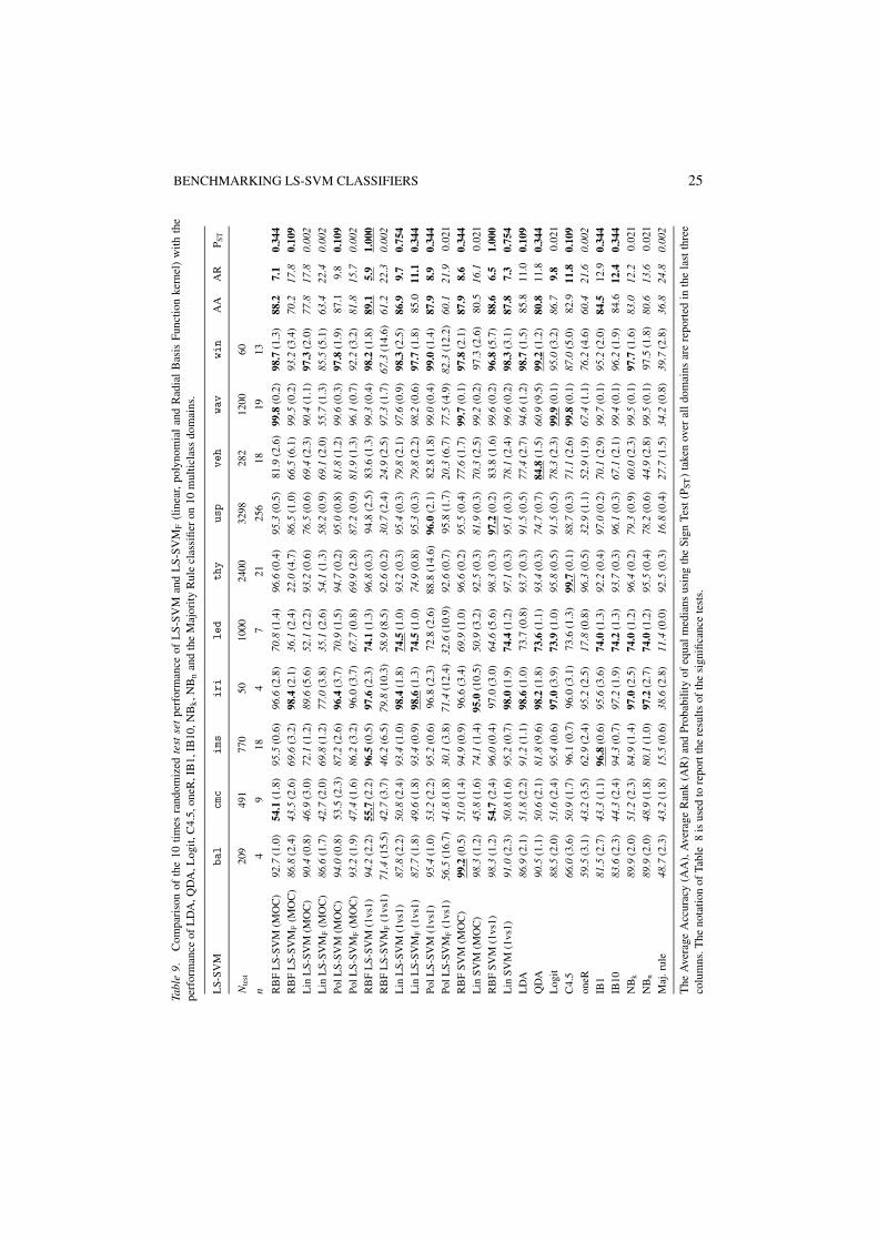
We report the performance of multiclass LS-SVMs on 10 multiclass categorization prob-lems. Each multiclass problem is decomposed into a set of binary classification problemsusing minimum output coding (MOC) and one-versus-one (1vs1) output coding. The samekernel types as for the binary domain were considered: RBF kernels, linear (Lin) and poly-nomial (Pol) kernels with degrees d = 2, . . . , 10. Both the performance of LS-SVM andLS-SVMF classifiers are reported. The MOC and 1vs1 output coding were also applied toSVM classifiers with linear and RBF kernels. As for the binary domains, we normalizedthe inputs to zero mean and unit variance (Bishop, 1995).
The experimental setup of the previous section is used: each binary classifier of themulticlass LS-SVM is designed on the first 2/3 of the data using 10-fold cross-validation,while the remaining 1/3 are put aside for testing. The selected regularization and kernelparameters3 were then fixed and 10 randomizations were conducted on each domain. Theaverage test set accuracies of the different LS-SVM and LS-SVMF classifiers, with RBF,Lin and Pol kernel (d = 2, . . . , 10) and using MOC and 1vs1 output coding, are reported inTable 9. The test set accuracies of the reference algorithms on the same randomizations arealso reported, where we remark that for the usp dataset the memory requirements for logitwere too high. Instead, we tabulated the performance of LDA instead of logit for this singlecase. The same statistical tests as in Section 7.3 were used to compare the performance ofthe different classifiers.
The use of QDA yields the best average test set accuracy on two domains, while LS-SVMswith 1vs1 coding using a RBF and Lin kernel and LS-SVMF with Lin kernel each yield thebest performance on one domain. SVMs with RBF kernel with MOC and 1vs1 coding yieldthe best performance on one domain each. Also C4.5, logit and IB1 each achieve one timethe best performance. The use of 1vs1 coding generally results into a better classificationaccuracy. Averaging over all 10 multiclass domains, the LS-SVM classifier with RBF kerneland 1vs1 output coding achieves the best average accuracy (AA) and average ranking, whileits performance is only on three domains significantly worse at 1% than the best algorithm.This performance is not significantly different from the SVM with RBF kernel and 1vs1output coding. Summarizing the different significant tests, RBF LS-SVM (MOC), Pol LS-SVM (MOC), Lin LS-SVM (1vs1), Lin LS-SVMF (1vs1), Pol LS-SVM (1vs1), RBF SVM(MOC), RBF SVM (1vs1), Lin SVM (1vs1), LDA, QDA, Logit, C4.5, IB1 and IB10 performnot significantly different at the 5% level. While NBk performed well on the binary domains,its average accuracy on the multiclass domains is never comparable at the 5% level for allthree tests. The overall results of Table 9 illustrate that the SVM and LS-SVM classifierwith RBF kernel using 1vs1 output coding consistently yield very good test set accuracieson the multiclass domains.
BENCHMARKING LS-SVM CLASSIFIERS 25Ta
ble
9.C
ompa
riso
nof
the
10tim
esra
ndom
ized
test
set
perf
orm
ance
ofL
S-SV
Man
dL
S-SV
MF
(lin
ear,
poly
nom
ial
and
Rad
ial
Bas
isFu
nctio
nke
rnel
)w
ithth
epe
rfor
man
ceof
LD
A,Q
DA
,Log
it,C
4.5,
oneR
,IB
1,IB
10,N
Bk,N
Bn
and
the
Maj
ority
Rul
ecl
assi
fier
on10
mul
ticla
ssdo
mai
ns.
LS-
SVM
bal
cmc
ims
iri
led
thy
usp
veh
wav
win
AA
AR
P ST
Nte
st20
949
177
050
1000
2400
3298
282
1200
60
n4
918
47
2125
618
1913
RB
FL
S-SV
M(M
OC
)92
.7(1
.0)
54.1
(1.8
)95
.5(0
.6)
96.6
(2.8
)70
.8(1
.4)
96.6
(0.4
)95
.3(0
.5)
81.9
(2.6
)99
.8(0
.2)
98.7
(1.3
)88
.27.
10.
344
RB
FL
S-SV
MF
(MO
C)
86.8
(2.4
)43
.5(2
.6)
69.6
(3.2
)98
.4(2
.1)
36.1
(2.4
)22
.0(4
.7)
86.5
(1.0
)66
.5(6
.1)
99.5
(0.2
)93
.2(3
.4)
70.2
17.8
0.10
9L
inL
S-SV
M(M
OC
)90
.4(0
.8)
46.9
(3.0
)72
.1(1
.2)
89.6
(5.6
)52
.1(2
.2)
93.2
(0.6
)76
.5(0
.6)
69.4
(2.3
)90
.4(1
.1)
97.3
(2.0
)77
.817
.80.
002
Lin
LS-
SVM
F(M
OC
)86
.6(1
.7)
42.7
(2.0
)69
.8(1
.2)
77.0
(3.8
)35
.1(2
.6)
54.1
(1.3
)58
.2(0
.9)
69.1
(2.0
)55
.7(1
.3)
85.5
(5.1
)63
.422
.40.
002
PolL
S-SV
M(M
OC
)94
.0(0
.8)
53.5
(2.3
)87
.2(2
.6)
96.4
(3.7
)70
.9(1
.5)
94.7
(0.2
)95
.0(0
.8)
81.8
(1.2
)99
.6(0
.3)
97.8
(1.9
)87
.19.
80.
109
PolL
S-SV
MF
(MO
C)
93.2
(1.9
)47
.4(1
.6)
86.2
(3.2
)96
.0(3
.7)
67.7
(0.8
)69
.9(2
.8)
87.2
(0.9
)81
.9(1
.3)
96.1
(0.7
)92
.2(3
.2)
81.8
15.7
0.00
2
RB
FL
S-SV
M(1
vs1)
94.2
(2.2
)55
.7(2
.2)
96.5
(0.5
)97
.6(2
.3)
74.1
(1.3
)96
.8(0
.3)
94.8
(2.5
)83
.6(1
.3)
99.3
(0.4
)98
.2(1
.8)
89.1
5.9
1.00
0R
BF
LS-
SVM
F(1
vs1)
71.4
(15.
5)42
.7(3
.7)
46.2
(6.5
)79
.8(1
0.3)
58.9
(8.5
)92
.6(0
.2)
30.7
(2.4
)24
.9(2
.5)
97.3
(1.7
)67
.3(1
4.6)
61.2
22.3
0.00
2
Lin
LS-
SVM
(1vs
1)87
.8(2
.2)
50.8
(2.4
)93
.4(1
.0)
98.4
(1.8
)74
.5(1
.0)
93.2
(0.3
)95
.4(0
.3)
79.8
(2.1
)97
.6(0
.9)
98.3
(2.5
)86
.99.
70.
754
Lin
LS-
SVM
F(1
vs1)
87.7
(1.8
)49
.6(1
.8)
93.4
(0.9
)98
.6(1
.3)
74.5
(1.0
)74
.9(0
.8)
95.3
(0.3
)79
.8(2
.2)
98.2
(0.6
)97
.7(1
.8)
85.0
11.1
0.34
4Po
lLS-
SVM
(1vs
1)95
.4(1
.0)
53.2
(2.2
)95
.2(0
.6)
96.8
(2.3
)72
.8(2
.6)
88.8
(14.
6)96
.0(2
.1)
82.8
(1.8
)99
.0(0
.4)
99.0
(1.4
)87
.98.
90.
344
PolL
S-SV
MF
(1vs
1)56
.5(1
6.7)
41.8
(1.8
)30
.1(3
.8)
71.4
(12.
4)32
.6(1
0.9)
92.6
(0.7
)95
.8(1
.7)
20.3
(6.7
)77
.5(4
.9)
82.3
(12.
2)60
.121
.90.
021
RB
FSV
M(M
OC
)99
.2(0
.5)
51.0
(1.4
)94
.9(0
.9)
96.6
(3.4
)69
.9(1
.0)
96.6
(0.2
)95
.5(0
.4)
77.6
(1.7
)99
.7(0
.1)
97.8
(2.1
)87
.98.
60.
344
Lin
SVM
(MO
C)
98.3
(1.2
)45
.8(1
.6)
74.1
(1.4
)95
.0(1
0.5)
50.9
(3.2
)92
.5(0
.3)
81.9
(0.3
)70
.3(2
.5)
99.2
(0.2
)97
.3(2
.6)
80.5
16.1
0.02
1
RB
FSV
M(1
vs1)
98.3
(1.2
)54
.7(2
.4)
96.0
(0.4
)97
.0(3
.0)
64.6
(5.6
)98
.3(0
.3)
97.2
(0.2
)83
.8(1
.6)
99.6
(0.2
)96
.8(5
.7)
88.6
6.5
1.00
0L
inSV
M(1
vs1)
91.0
(2.3
)50
.8(1
.6)
95.2
(0.7
)98
.0(1
.9)
74.4
(1.2
)97
.1(0
.3)
95.1
(0.3
)78
.1(2
.4)
99.6
(0.2
)98
.3(3
.1)
87.8
7.3
0.75
4L
DA
86.9
(2.1
)51
.8(2
.2)
91.2
(1.1
)98
.6(1
.0)
73.7
(0.8
)93
.7(0
.3)
91.5
(0.5
)77
.4(2
.7)
94.6
(1.2
)98
.7(1
.5)
85.8
11.0
0.10
9Q
DA
90.5
(1.1
)50
.6(2
.1)
81.8
(9.6
)98
.2(1
.8)
73.6
(1.1
)93
.4(0
.3)
74.7
(0.7
)84
.8(1
.5)
60.9
(9.5
)99
.2(1
.2)
80.8
11.8
0.34
4L
ogit
88.5
(2.0
)51
.6(2
.4)
95.4
(0.6
)97
.0(3
.9)
73.9
(1.0
)95
.8(0
.5)
91.5
(0.5
)78
.3(2
.3)
99.9
(0.1
)95
.0(3
.2)
86.7
9.8
0.02
1
C4.
566
.0(3
.6)
50.9
(1.7
)96
.1(0
.7)
96.0
(3.1
)73
.6(1
.3)
99.7
(0.1
)88
.7(0
.3)
71.1
(2.6
)99
.8(0
.1)
87.0
(5.0
)82
.911
.80.
109
oneR
59.5
(3.1
)43
.2(3
.5)
62.9
(2.4
)95
.2(2
.5)
17.8
(0.8
)96
.3(0
.5)
32.9
(1.1
)52
.9(1
.9)
67.4
(1.1
)76
.2(4
.6)
60.4
21.6
0.00
2
IB1
81.5
(2.7
)43
.3(1
.1)
96.8
(0.6
)95
.6(3
.6)
74.0
(1.3
)92
.2(0
.4)
97.0
(0.2
)70
.1(2
.9)
99.7
(0.1
)95
.2(2
.0)
84.5
12.9
0.34
4IB
1083
.6(2
.3)
44.3
(2.4
)94
.3(0
.7)
97.2
(1.9
)74
.2(1
.3)
93.7
(0.3
)96
.1(0
.3)
67.1
(2.1
)99
.4(0
.1)
96.2
(1.9
)84
.612
.40.
344
NB
k89
.9(2
.0)
51.2
(2.3
)84
.9(1
.4)
97.0
(2.5
)74
.0(1
.2)
96.4
(0.2
)79
.3(0
.9)
60.0
(2.3
)99
.5(0
.1)
97.7
(1.6
)83
.012
.20.
021
NB
n89
.9(2
.0)
48.9
(1.8
)80
.1(1
.0)
97.2
(2.7
)74
.0(1
.2)
95.5
(0.4
)78
.2(0
.6)
44.9
(2.8
)99
.5(0
.1)
97.5
(1.8
)80
.613
.60.
021
Maj
.rul
e48
.7(2
.3)
43.2
(1.8
)15
.5(0
.6)
38.6
(2.8
)11
.4(0
.0)
92.5
(0.3
)16
.8(0
.4)
27.7
(1.5
)34
.2(0
.8)
39.7
(2.8
)36
.824
.80.
002
The
Ave
rage
Acc
urac
y(A
A),
Ave
rage
Ran
k(A
R)
and
Prob
abili
tyof
equa
lm
edia
nsus
ing
the
Sign
Test
(PST
)ta
ken
over
all
dom
ains
are
repo
rted
inth
ela
stth
ree
colu
mns
.The
nota
tion
ofTa
ble
8is
used
tore
port
the
resu
ltsof
the
sign
ifica
nce
test
s.
26 T. VAN GESTEL ET AL.
7.5. LS-SVM sparse approximation procedure
The sparseness property of SVMs is lost in LS-SVMs by the use of a 2-norm. While thegeneralization capacity is still controlled by the regularization term, the use of a smallernumber of support vectors may be interesting to reduce the computational cost of evaluatingthe classifier for new inputs x . We illustrate the sparse approximation procedure (Suykens &Vandewalle, 1999b; 1999c; Suykens et al., 2002) of Section 4 on 10 datasets for LS-SVMswith RBF kernel.
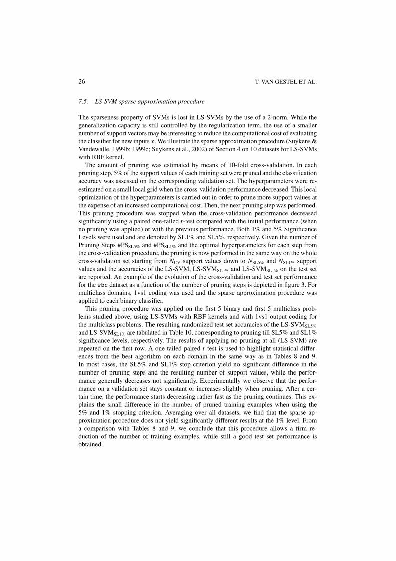
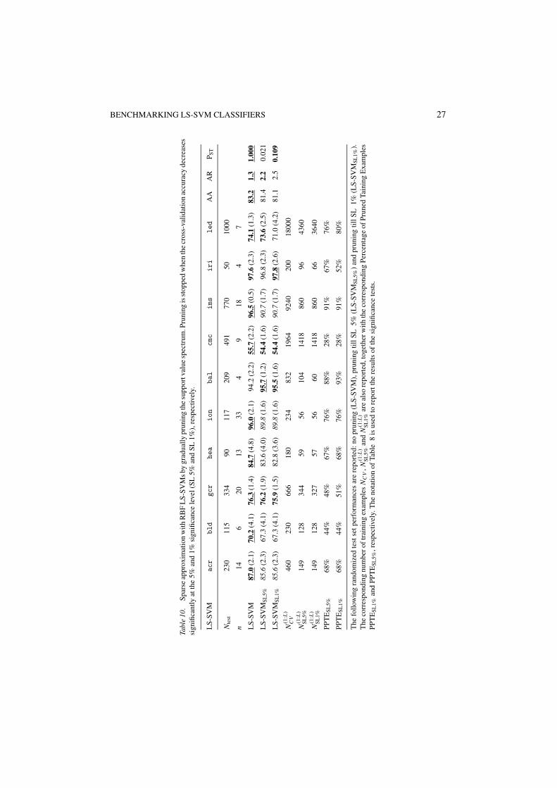
The amount of pruning was estimated by means of 10-fold cross-validation. In eachpruning step, 5% of the support values of each training set were pruned and the classificationaccuracy was assessed on the corresponding validation set. The hyperparameters were re-estimated on a small local grid when the cross-validation performance decreased. This localoptimization of the hyperparameters is carried out in order to prune more support values atthe expense of an increased computational cost. Then, the next pruning step was performed.This pruning procedure was stopped when the cross-validation performance decreasedsignificantly using a paired one-tailed t-test compared with the initial performance (whenno pruning was applied) or with the previous performance. Both 1% and 5% SignificanceLevels were used and are denoted by SL1% and SL5%, respectively. Given the number ofPruning Steps #PSSL5% and #PSSL1% and the optimal hyperparameters for each step fromthe cross-validation procedure, the pruning is now performed in the same way on the wholecross-validation set starting from NCV support values down to NSL5% and NSL1% supportvalues and the accuracies of the LS-SVM, LS-SVMSL5% and LS-SVMSL1% on the test setare reported. An example of the evolution of the cross-validation and test set performancefor the wbc dataset as a function of the number of pruning steps is depicted in figure 3. Formulticlass domains, 1vs1 coding was used and the sparse approximation procedure wasapplied to each binary classifier.
This pruning procedure was applied on the first 5 binary and first 5 multiclass prob-lems studied above, using LS-SVMs with RBF kernels and with 1vs1 output coding forthe multiclass problems. The resulting randomized test set accuracies of the LS-SVMSL5%
and LS-SVMSL1% are tabulated in Table 10, corresponding to pruning till SL5% and SL1%significance levels, respectively. The results of applying no pruning at all (LS-SVM) arerepeated on the first row. A one-tailed paired t-test is used to highlight statistical differ-ences from the best algorithm on each domain in the same way as in Tables 8 and 9.In most cases, the SL5% and SL1% stop criterion yield no significant difference in thenumber of pruning steps and the resulting number of support values, while the perfor-mance generally decreases not significantly. Experimentally we observe that the perfor-mance on a validation set stays constant or increases slightly when pruning. After a cer-tain time, the performance starts decreasing rather fast as the pruning continues. This ex-plains the small difference in the number of pruned training examples when using the5% and 1% stopping criterion. Averaging over all datasets, we find that the sparse ap-proximation procedure does not yield significantly different results at the 1% level. Froma comparison with Tables 8 and 9, we conclude that this procedure allows a firm re-duction of the number of training examples, while still a good test set performance isobtained.
BENCHMARKING LS-SVM CLASSIFIERS 27
Tabl
e10
.Sp
arse
appr
oxim
atio
nw
ithR
BF
LS-
SVM
sby
grad
ually
prun
ing
the
supp
ortv
alue
spec
trum
.Pru
ning
isst
oppe
dw
hen
the
cros
s-va
lidat
ion
accu
racy
decr
ease
ssi
gnifi
cant
lyat
the
5%an
d1%
sign
ifica
nce
leve
l(SL
5%an
dSL
1%),
resp
ectiv
ely.
LS-
SVM
acr
bld
gcr
hea
ion
bal
cmc
ims
iri
led
AA
AR
P ST
Nte
st23
011
533
490
117
209
491
770
5010
00
n14
620
1333
49
184
7
LS-
SVM
87.0
(2.1
)70
.2(4
.1)
76.3
(1.4
)84
.7(4
.8)
96.0
(2.1
)94
.2(2
.2)
55.7
(2.2
)96
.5(0
.5)
97.6
(2.3
)74
.1(1
.3)
83.2
1.3
1.00
0
LS-
SVM
SL5%
85.6
(2.3
)67
.3(4
.1)
76.2
(1.9
)83
.6(4
.0)
89.8
(1.6
)95
.7(1
.2)
54.4
(1.6
)90
.7(1
.7)
96.8
(2.3
)73
.6(2
.5)
81.4
2.2
0.02
1
LS-
SVM
SL1%
85.6
(2.3
)67
.3(4
.1)
75.9
(1.5
)82
.8(3
.6)
89.8
(1.6
)95
.5(1
.6)
54.4
(1.6
)90
.7(1
.7)
97.8
(2.6
)71
.0(4
.2)
81.1
2.5
0.10
9
N(1
:L)
CV
460
230
666
180
234
832
1964
9240
200
1800
0
N(1
:L)
SL5%
149
128
344
5956
104
1418
860
9643
60
N(1
:L)
SL1%
149
128
327
5756
6014
1886
066
3640
PPT
ESL
5%68
%44
%48
%67
%76
%88
%28
%91
%67
%76
%
PPT
ESL
1%68
%44
%51
%68
%76
%93
%28
%91
%52
%80
%
The
follo
win
gra
ndom
ized
test
setp
erfo
rman
ces
are
repo
rted
:no
prun
ing
(LS-
SVM
),pr
unin
gtil
lSL
5%(L
S-SV
MSL
5%)
and
prun
ing
tillS
L1%
(LS-
SVM
SL1%
).T
heco
rres
pond
ing
num
bero
ftra
inin
gex
ampl
esN
CV
,N(1
:L)
SL5%
and
N(1
:L)
SL1%
are
also
repo
rted
,tog
ethe
rwith
the
corr
espo
ndin
gPe
rcen
tage
ofPr
uned
Tain
ing
Exa
mpl
esPP
TE
SL1%
and
PPT
ESL
5%,r
espe
ctiv
ely.
The
nota
tion
ofTa
ble
8is
used
tore
port
the
resu
ltsof
the
sign
ifica
nce
test
s.
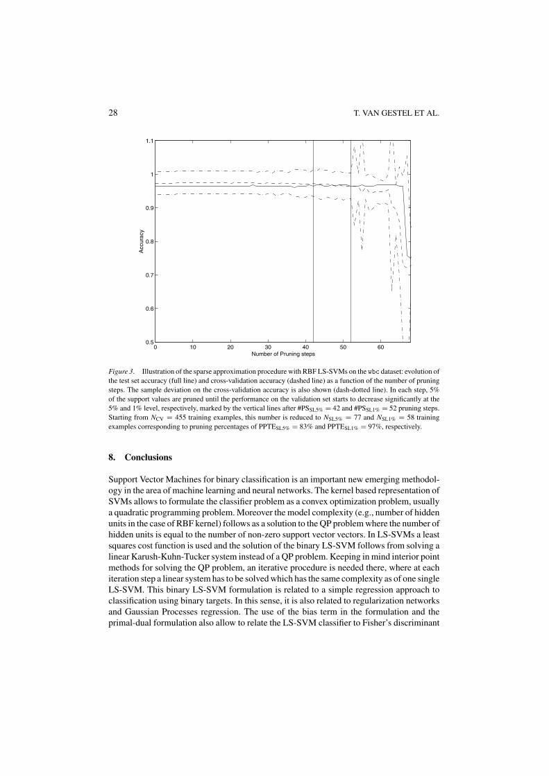
28 T. VAN GESTEL ET AL.
0 10 20 30 40 50 600.5
0.6
0.7
0.8
0.9
1
1.1
Number of Pruning steps
Acc
urac
y
Figure 3. Illustration of the sparse approximation procedure with RBF LS-SVMs on the wbc dataset: evolution ofthe test set accuracy (full line) and cross-validation accuracy (dashed line) as a function of the number of pruningsteps. The sample deviation on the cross-validation accuracy is also shown (dash-dotted line). In each step, 5%of the support values are pruned until the performance on the validation set starts to decrease significantly at the5% and 1% level, respectively, marked by the vertical lines after #PSSL5% = 42 and #PSSL1% = 52 pruning steps.Starting from NCV = 455 training examples, this number is reduced to NSL5% = 77 and NSL1% = 58 trainingexamples corresponding to pruning percentages of PPTESL5% = 83% and PPTESL1% = 97%, respectively.
8. Conclusions
Support Vector Machines for binary classification is an important new emerging methodol-ogy in the area of machine learning and neural networks. The kernel based representation ofSVMs allows to formulate the classifier problem as a convex optimization problem, usuallya quadratic programming problem. Moreover the model complexity (e.g., number of hiddenunits in the case of RBF kernel) follows as a solution to the QP problem where the number ofhidden units is equal to the number of non-zero support vector vectors. In LS-SVMs a leastsquares cost function is used and the solution of the binary LS-SVM follows from solving alinear Karush-Kuhn-Tucker system instead of a QP problem. Keeping in mind interior pointmethods for solving the QP problem, an iterative procedure is needed there, where at eachiteration step a linear system has to be solved which has the same complexity as of one singleLS-SVM. This binary LS-SVM formulation is related to a simple regression approach toclassification using binary targets. In this sense, it is also related to regularization networksand Gaussian Processes regression. The use of the bias term in the formulation and theprimal-dual formulation also allow to relate the LS-SVM classifier to Fisher’s discriminant
BENCHMARKING LS-SVM CLASSIFIERS 29
analysis in the feature space, also known as Kernel Fisher Discriminant Analysis. Multi-class categorization problems are reformulated as a set of binary classification problemsusing, e.g., minimum output coding and one-versus-one output coding. We have shown ontwenty UCI binary and multiclass benchmark datasets that the SVM and LS-SVM formu-lation in combination with standard cross-validation methods for hyperparameter selectionare performing consistently very well on all tried datasets in comparison with many othermethods. We have also verified that the lack of sparseness of LS-SVMs can be circum-vented by applying sparse approximation in a second stage by pruning less important datafrom the sorted support value spectrum. In all experiments LS-SVMs with RBF kerneland cross-validation tuning of the two hyperparameters are performing well and at least asgood as LS-SVMs with linear kernel which, in combination with the sparse approximationprocedure, also offers the possibility for knowledge discovery in the datasets.
Acknowledgments
T. Van Gestel and J.A.K. Suykens are a Research Assistant and Postdoctoral Researcherwith the FWO Flanders, respectively. S. Viaene is researcher at LIRIS with the KBC In-surance Research Chair. G. Dedene is a co-founder of the KBC Insurance Research Chair.This work was carried out at the ESAT laboratory, the Interdisciplinary Center of NeuralNetworks ICNN and the institute LIRIS of the K.U.Leuven and supported by grants andprojects from the Flemish Gov.: (Research council KUL: Grants, GOA-Mefisto 666; FWO-Flanders: Grants, res. proj. (G.0262.97, G.0135.95, G.0115.01, G.0197.02, G.0407.02) andcomm. (ICCoS and ANMMM); AWI: Bil. Int. Coll.; IWT: STWW Eureka SINOPSYS, IM-PACT, FLiTe; STWW Genprom, GBOU McKnow; from the Belgian Fed. Gov. (Interuniv.Attr. Poles: IUAP-P4/02, P4/24; Program Dur. Dev.); from the Eur. Comm.: (TMR Netw.(Alapedes, Niconet); Science: ERNSI). The work is also carried out in the framework ofthe KBC Insurance Research Chair, set up in September 1997 as a pioneering cooperationbetween LIRIS and KBC Insurance.
Notes
1. The square root√
n of the number of inputs n is considered in the grid � (Step 2) since ‖x − xi ‖22 in the RBF
kernel is proportional to n.2. The matlab SVM toolbox (Cawley, 2000) with SMO solver (Platt, 1998) was used to train and evaluate the
Vapnik SVM classifier. The C4.5, IB1, IB10, Naive Bayes and oneR algorithms were implemented using theWeka workbench (Witten & Frank, 2000), while the Discriminant Analysis Toolbox (M. Kiefte) for Matlabwas applied for LDA, QDA and logit.
3. The corresponding optimal values for the hyperparameters are not reported, because of the large number ofbinary classifiers for some datasets.
References
Aha, D., & Kibler, D. (1991). Instance-based learning algorithms. Machine Learning, 6, 37–66.Allwein, E. L., Schapire, R. E., & Singer, Y. (2000). Reducing multiclass to binary: A unifying approach for
margin classifiers. Journal of Machine Learning Research, 1, 113–141.
30 T. VAN GESTEL ET AL.
Baudat, G., & Anouar, F. (2000). Generalized discriminant analysis using a Kernel approach. Neural Computation,12, 2385–2404.
Bay, S. D. (1999). Nearest neighbor classification from multiple feature subsets. Intelligent Data Analysis, 3,191–209.
Bishop, C. M. (1995). Neural Networks for Pattern Recognition. Oxford University Press.Blake, C. L., & Merz, C. J. (1998). UCI Repository of machine learning databases [http://www.ics.
uci.edu/˜mlearn/MLRepository.html]. Irvine, CA: University of California, Dept. of Information and ComputerScience.
Boser, B., Guyon, I., & Vapnik, V. (1992). A training algorithm for optimal margin classifiers. In Proc. of the FifthAnnual Workshop on Computational Learning Theory (pp. 144–152). Pittsburgh: ACM.
Bradley, P. S., & Mangasarian, O. L. (1998). Feature selection via concave minimization and support vectormachines. In J. Shavlik (ed.), Machine Learning Proc. of the Fifteenth Int. Conf. (ICML’98) (pp. 82–90).Morgan Kaufmann, San Francisco, California.
Breiman, L., Friedman, J., Olshen, R., & Stone, C. (1984). Classification and Regression Trees. New York:Chapman and Hall.
Cawley, G. C. (2000). MATLAB Support Vector Machine Toolbox (v0.54β). [http://theoval.sys.uea.ac.uk/∼gcc/svm/toolbox]. University of East Anglia, School of Information Systems, Norwich, Norfolk, U.K.
Cristianini, N., & Shawe-Taylor, J. (2000) An Introduction to Support Vector Machines. Cambridge UniversityPress.
De Groot, M. H. (1986). Probability and Statistics, 2nd ed. Reading, MA: Addison-Wesley.Domingos, P. (1996). Unifying instance-based and rule-based induction. Machine Learning, 24, 141–168.Dietterich, T. G. (1998). Approximate statistical tests for comparing supervised classification learning algorithms.
Neural Computation, 10, 1895–1924.Dietterich, T. G., & Bakiri, G. (1995). Solving multiclass learning problems via error-correcting output codes.
Journal of Artificial Intelligence Research, 2, 263–286.Duda, R. O., & Hart, P. E. (1973), Pattern Classification and Scene Analysis. New York: John Wiley.Evgeniou, T., Pontil, M., & Poggio, T. (2001). Regularization networks and support vector machines. Advances
in Computational Mathematics, 13, 1–50.Fisher, R. A. (1936). The use of multiple measurements in taxonomic problems. Annals of Eugenics, 7:2, 179–188.Friedman, J. (1989). Regularized discriminant analysis. Journal of the American Statistical Association, 84, 165–
175.Girosi, F. (1998). An equivalence between sparse approximation and support vector machines. Neural Computa-
tion, 10, 1455–1480.Golub, G. H., & Van Loan, C. F. (1989). Matrix Computations. Baltimore MD: Johns Hopkins University Press.Hassibi, B., & Stork, D. G. (1993). Second order derivatives for network pruning: Optimal brain surgeon. In
Hanson, Cowan, & Giles (Eds.), Advances in Neural Information Processing Systems (Vol. 5). San Mateo, CA:Morgan Kaufmann.
Hastie, T., & Tibshirani, R. (1998). Classification by pairwise coupling. The Annals of Statistics, 26, 451–471.Holte, R. C. (1993). Very simple classification rules perform well on most commonly used datasets. Machine
Learning, 11, 63–90.John, G. H., & Langley, P. (1995). Estimating continuous distributions in Bayesian classifiers. In Proceedings of
the Eleventh Conference on Uncertainty in Artificial Intelligence (pp. 338–345). Montreal, Quebec, MorganKaufmann.
Kwok, J. T. (2000). The evidence framework applied to support vector machines. IEEE Trans. on Neural Networks,10:5, 1018–1031.
Le Cun, Y., Denker, J. S., & Solla, S. A. (1990). Optimal brain damage. In Touretzky (Ed.), Advances in NeuralInformation Processing Systems (Vol. 2). San Mateo, CA: Morgan Kaufmann.
Lim, T.-S., Loh, W.-Y., & Shih, Y.-S. (2000). A comparison of prediction accuracy, complexity, and training timeof thirty-three old and new classification algorithms. Machine Learning, 40:3, 203–228.
MacKay, D. J. C. (1995). Probable networks and plausible predictions—A review of practical Bayesian methodsfor supervised neural networks. Network: Computation in Neural Systems, 6, 469–505.
Mika, S., Ratsch, G., Weston, J., Scholkopf, B., & Muller, K.-R. (1999). Fisher discriminant analysis with Kernels.In Proc. IEEE Neural Networks for Signal Processing Workshop 1999, NNSP 99.
BENCHMARKING LS-SVM CLASSIFIERS 31
Navia-Vazquez, A., Perez-Cruz, F., Artes-Rodriguez, A., Figueiras-Vidal, A. R. (2001). Weighted least squarestraining of support vector classifiers leading to compact and adaptive schemes. IEEE Transactions on NeuralNetworks, 12, 1047–1059.
Platt, J. (1998). Fast training of support vector machines using sequential minimal optimization. In B. Scholkopf,C. J. C. Burges, & A. J. Smola (Eds.), Advances in Kernel Methods—Support Vector Learning. Cambridge,MA.
Quinlan, J. (1993). C4.5 Programs for Machine Learning. Morgan Kaufmann.Rao, P. (1983) Nonparametric Functional Estimation. Orlando: Academic Press.Ripley, B. D. (1996). Pattern Classification and Neural Networks. Cambridge.Saunders, C., Gammerman, A., & Vovk, V. (1998). Ridge regression learning algorithm in dual variables. In
Proc. of the 15th Int. Conf. on Machine Learning ICML-98 (pp. 515–521). Madison-Wisconsin: MorganKaufmann.
Scholkopf, B., Sung, K.-K., Burges, C., Girosi, F., Niyogi, P., Poggio, T., & Vapnik, V. (1997). Comparingsupport vector machines with Gaussian Kernels to radial basis function classifiers. IEEE Transactions on SignalProcessing, 45, 2758–2765.
Scholkopf, B., Burges, C., & Smola, A. (Eds.), (1998). Advances in Kernel Methods—Support Vector Learning.MIT Press.
Sejnowski, T. J., & Rosenberg, C. R. (1987). Parallel networks that learn to pronounce English text. Journal ofComplex Systems, 1:1, 145–168.
Smola, A., Scholkopf, B., & Muller, K.-R. (1998). The connection between regularization operators and supportvector kernels. Neural Networks, 11, 637–649.
Smola, A. (1999). Learning with Kernels. PhD Thesis, published by: GMD, Birlinghoven.Suykens, J. A. K., & Vandewalle, J. (Eds.) (1998). Nonlinear Modeling: Advanced Black-Box Techniques. Boston:
Kluwer Academic Publishers.Suykens, J. A. K., & Vandewalle, J. (1999a). Training multilayer perceptron classifiers based on a modified support
vector method. IEEE Transactions on Neural Networks, 10, 907–912.Suykens, J. A. K., & Vandewalle, J. (1999b). Least squares support vector machine classifiers. Neural Processing
Letters, 9, 293–300.Suykens, J. A. K., Lukas, L., Van Dooren, P., De Moor, B., & Vandewalle, J. (1999). Least squares support vector
machine classifiers: A large scale algorithm. In Proc. of the European Conf. on Circuit Theory and Design(ECCTD’99) (pp. 839–842).
Suykens, J. A. K., & Vandewalle, J. (1999c). Multiclass least squares support vector machines. In Proc. of the Int.Joint Conf. on Neural Networks (IJCNN’99), Washington, DC.
Suykens, J. A. K., De Brabanter, J., Lukas, L., & Vandewalle, J. (2002). Weighted least squares support vectormachines: Robustness and sparse approximation. Neurocomputing, 48:1–4, 85–105.
Suykens, J. A. K., & Vandewalle, J. (2000). Recurrent least squares support vector machines. IEEE Transactionson Circuits and Systems-I, 47, 1109–1114.
Suykens, J. A. K., Vandewalle, J., & De Moor, B. (2001). Optimal control by least squares support vector machines.Neural Networks, 14, 23–35.
Tipping, M. E. (2001). Sparse Bayesian learning and the relevance vector machine. Journal of Machine LearningResearch, 1, 211–244.
Utschick, W. (1998). A regularization method for non-trivial codes in polychotomous classification. InternationalJournal of Pattern Recognition and Artificial Intelligence, 12, 453–474.
Van Gestel, T., Suykens, J. A. K., Baestaens, D.-E., Lambrechts, A., Lanckriet, G., Vandaele, B., De Moor, B., &Vandewalle, J. (2001). Predicting financial time series using least squares support vector machines within theevidence framework. IEEE Transactions on Neural Networks, (Special Issue on Financial Engineering), 12,809–821.
Van Gestel, T., Suykens, J. A. K., Lanckriet, G., Lambrechts, A., De Moor, B., & Vandewalle, J. (2002). A Bayesianframework for least squares support vector machine classifiers. Neural Computation, 14, 1115–1148.
Vapnik, V. (1995). The Nature of Statistical Learning Theory. New-York: Springer-Verlag.Vapnik, V. (1998a). Statistical Learning Theory. New-York: John Wiley.Vapnik, V. (1998b). The support vector method of function estimation. In J. A. K. Suykens, & J. Vandewalle,
(Eds.), Nonlinear Modeling: Advanced Black-box Techniques. Boston: Kluwer Academic Publishers.
32 T. VAN GESTEL ET AL.
Viaene, S., Baesens, B., Van Gestel, T., Suykens, J. A. K., Van den Poel, D., Vanthienen, J., De Moor, B., &Dedene, G. (2001). Knowledge discovery in a direct marketing case using least squares support vector machineclassifiers. International Journal of Intelligent Systems, 9, 1023–1036.
Williams, C. K. I. (1998). Prediction with Gaussian processes: From linear regression to linear prediction andbeyond. In M. I. Jordan (Ed.), Learning and Inference in Graphical Models. Kluwer Academic Press.
Witten, I. H., & Frank, E. (2000). Data Mining: Practical Machine Learning Tools and Techniques with JavaImplementations. San Francisco: Morgan Kaufmann.
Received March 9, 2001Revised October 22, 2001Accepted May 27, 2002Final manuscript June 12, 2002


![Robust energy-based least squares twin support vector machines · Robust energy-based least squares twin support vector machines 175 support vector machine (LSTSVM) [14] has been](https://img.pdfslide.net/doc/110x75/5b47bc007f8b9aa4148d0ec7/robust-energy-based-least-squares-twin-support-vector-machines-robust-energy-based.jpg)