Embed Size (px)
Citation preview

Regularized Least Squares and SupportVector Machines
Lorenzo Rosasco
9.520 Class 06
L. Rosasco RLS and SVM

About this class
Goal To introduce two main examples of Tikhonovregularization, deriving and comparing theircomputational properties.
L. Rosasco RLS and SVM

Basics: Data
Training set: S = {(x1, y1), . . . , (xn, yn)}.Inputs: X = {x1, . . . , xn}.Labels: Y = {y1, . . . , yn}.
L. Rosasco RLS and SVM

Basics: RKHS, Kernel
RKHS H with a positive semidefinite kernel function K :
linear: K (xi , xj) = xTi xj
polynomial: K (xi , xj) = (xTi xj + 1)d
gaussian: K (xi , xj) = exp
(−||xi − xj ||2
σ2
)
Define the kernel matrix K to satisfy Kij = K (xi , xj).The kernel function with one argument fixed isKx = K (x , ·).Given an arbitrary input x∗, Kx∗ is a vector whose i th entryis K (xi , x∗).
L. Rosasco RLS and SVM

Tikhonov Regularization
We are interested into studying Tikhonov Regularization
argminf∈H
{n∑
i=1
V (yi , f (xi))2 + λ‖f‖2H}.
L. Rosasco RLS and SVM

Representer Theorem
The representer theorem guarantees that the solution can bewritten as
f =n∑
j=1
cjKxj
for some c = (c1, . . . , cn) ∈ Rn.So Kc is a vector whose i th element is f (xi):
f (xi) =n∑
j=1
cjKxi (xj) =n∑
j=1
cjKij
and ‖f‖2H = cT Kc.
L. Rosasco RLS and SVM

RKHS Norm and Representer Theorem
Since f =∑n
j=1 cjKxj , then
‖f‖2H = 〈f , f 〉H
= 〈n∑
i=1
ciKxi ,
n∑j=1
cjKxj 〉H
=n∑
i=1
n∑j=1
cicj〈Kxi ,Kxj 〉H
=n∑
i=1
n∑j=1
cicjK (xi , xj) = ctKc
L. Rosasco RLS and SVM

Plan
RLSdual problemregularization pathlinear case
SVMdual problemlinear casehistorical derivation
L. Rosasco RLS and SVM

The RLS problem
Goal: Find the function f ∈ H that minimizes the weighted sumof the square loss and the RKHS norm
argminf∈H
{12
n∑i=1
(f (xi)− yi)2 +
λ
2||f ||2H}.
L. Rosasco RLS and SVM
RLS and Representer Theorem
Using the representer theorem the RLS problem is:
argminf∈H
12‖Y− Kc‖22 +
λ
2cT Kc
The above functional is differentiable, we can find the minimumsetting the gradient w.r.t c to 0:
−K(Y− Kc) + λKc = 0(K + λI)c = Y
c = (K + λI)−1Y
We find c by solving a system of linear equations.
L. Rosasco RLS and SVM
RLS and Representer Theorem
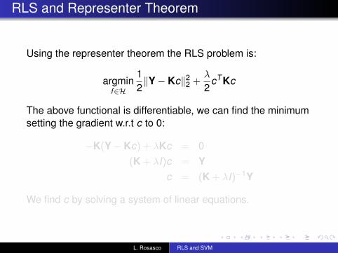
Using the representer theorem the RLS problem is:
argminf∈H
12‖Y− Kc‖22 +
λ
2cT Kc
The above functional is differentiable, we can find the minimumsetting the gradient w.r.t c to 0:
−K(Y− Kc) + λKc = 0(K + λI)c = Y
c = (K + λI)−1Y
We find c by solving a system of linear equations.
L. Rosasco RLS and SVM

Solving RLS for fixed Parameters
(K + λI)c = Y.
The matrix K + λI is symmetric positive definite, so theappropriate algorithm is Cholesky factorization.In Matlab, the “slash” operator seems to be using Cholesky,so you can just write c = (K + l ∗ I)\Y, but to be safe, (or inoctave), I suggest R = chol(K + l ∗ I); c = (R\(R’\Y));.
The above algorithm has complexity O(n3).
L. Rosasco RLS and SVM

The RLS Solution, Comments
c = (K + λI)−1Y
The prediction at a new input x∗ is:
f (x∗) =n∑
j=1
cjKxj (x∗)
= Kx∗c= Kx∗G−1Y,
where G = K + λI.Note that the above operation is O(n2).
L. Rosasco RLS and SVM

RLS Regularization Path
Typically we have to choose λ and hence to compute thesolutions corresponding to different values of λ.
Is there a more efficent method than solvingc(λ) = (K + λI)−1Y anew for each λ?Form the eigendecomposition K = QΛQT , where Λ isdiagonal with Λii ≥ 0 and QQT = I.Then
G = K + λI= QΛQT + λI= Q(Λ + λI)QT ,
which implies that G−1 = Q(Λ + λI)−1QT .
L. Rosasco RLS and SVM

RLS Regularization Path Cont’d
O(n3) time to solve one (dense) linear system, or tocompute the eigendecomposition (constant is maybe 4xworse). Given Q and Λ, we can find c(λ) in O(n2) time:
c(λ) = Q(Λ + λI)−1QT Y,
noting that (Λ + λI) is diagonal.Finding c(λ) for many λ’s is (essentially) free!
L. Rosasco RLS and SVM

The Linear Case
The linear kernel is K (xi , xj) = xTi xj .
The linear kernel offers many advantages for computation.Key idea: we get a decomposition of the kernel matrix forfree: K = XXT .In the linear case, we will see that we have two differentcomputation options.
L. Rosasco RLS and SVM

Linear kernel, linear function
With a linear kernel, the function we are learning is linear aswell:
f (x∗) = Kx∗c= xT
∗ XT c= xT
∗ w ,
where we define w to be XT c.
L. Rosasco RLS and SVM

Linear kernel cont.
For the linear kernel,
minc∈Rn
12||Y− Kc||22 +
λ
2cT Kc
= minc∈Rn
12||Y− XXT c||22 +
λ
2cT XXT c
= minw∈Rd
12||Y− Xw ||22 +
λ
2||w ||22.
Taking the gradient with respect to w and setting it to zero
XT Xw − XT Y + λw = 0
we getw = (XT X + λI)−1XT Y.
L. Rosasco RLS and SVM

Solution for fixed parameter
w = (XT X + λI)−1XT Y.
Choleski decomposition allows to solve the above problem inO(d3) for any fixed λ.
We can work with the covariance matrix XT X ∈ Rd×d .The algorithm is identical to solving a general RLS problemreplacing the kernel matrix by XT X and the labels vector byXT y .
We can classify new points in O(d) time, using w , rather thanhaving to compute a weighted sum of n kernel products (whichwill usually cost O(nd) time).
L. Rosasco RLS and SVM

Regularization Path via SVD
To compute solutions corresponding to multiple values of λ wecan again consider an eigend-ecomposition/svd.The economy-size SVD of X can be written as X = USV T , withU ∈ Rn×d , S ∈ Rd×d , V ∈ Rd×d , UT U = V T V = VV T = Id , andS diagonal and positive semidefinite. (Note that UUT 6= In).
We need O(nd) memory to store the data in the first place.The (economy-sized) SVD also requires O(nd) memory,and O(nd2) time.
Compared to the nonlinear case, we have replaced an O(n)with an O(d), in both time and memory. If n >> d , this canrepresent a huge savings.
L. Rosasco RLS and SVM

Summary So Far
When can we solve one RLS problem? (I.e. what are thebottlenecks?)We need to form K, which takes O(n2d) time and O(n2)memory. We need to perform a Cholesky factorization oran eigendecomposition of K, which takes O(n3) time.In the linear case we have replaced an O(n) with an O(d),in both time and memory. If n >> d , this can represent ahuge savings.Usually, we run out of memory before we run out oftime.The practical limit on today’s workstations is(more-or-less) 10,000 points (using Matlab).
L. Rosasco RLS and SVM

Parting Shot
“You should be asking how the answers will be used and whatis really needed from the computation. Time and time againsomeone will ask for the inverse of a matrix when all that isneeded is the solution of a linear system; for an interpolatingpolynomial when all that is needed is its values at some point;for the solution of an ODE at a sequence of points when all thatis needed is the limiting, steady-state value. A commoncomplaint is that least squares curve-fitting couldn’t possiblywork on this data set and some more complicated method isneeded; in almost all such cases, least squares curve-fitting willwork just fine because it is so very robust.”
Leader, Numerical Analysis and Scientific Computation
L. Rosasco RLS and SVM

Plan
RLSdual problemregularization pathlinear case
SVMdual problemlinear casehistorical derivation
L. Rosasco RLS and SVM

The Hinge Loss
The support vector machine for classification arises consideringthe hinge loss
V (f (x , y)) ≡ (1− yf (x))+,
where (s)+ ≡ max(s,0).
−3 −2 −1 0 1 2 3
0
0.5
1
1.5
2
2.5
3
3.5
4
y * f(x)
Hin
ge L
oss
L. Rosasco RLS and SVM

SVM Standard Notation
With the hinge loss, our regularization problem becomes
argminf∈H
1n
n∑i=1
(1− yi f (xi))+ + λ‖f‖2H.
In most of the SVM literature, the problem is written as
argminf∈H
Cn∑
i=1
V (yi , f (xi)) +12‖f‖2H.
The formulations are equivalent setting C = 12λn .
This problem is non-differentiable (because of the “kink” in V ).
L. Rosasco RLS and SVM

Slack Variables Formulation
We rewrite the functional using slack variables ξi .
argminf∈H
C∑n
i=1 ξi + 12‖f‖
2H
subject to : ξi ≥ 1− yi f (xi) i = 1, . . . ,nξi ≥ 0 i = 1, . . . ,n
Applying the representer theorem we get a constrainedquadratic programming problem:
argminc∈Rn,ξ∈Rn
C∑n
i=1 ξi + 12cT Kc
subject to : ξi ≥ 1− yi∑n
j=1 cjK (xi , xj) i = 1, . . . ,nξi ≥ 0 i = 1, . . . ,n
L. Rosasco RLS and SVM

How to Solve?
argminc∈Rn,ξ∈Rn
C∑n
i=1 ξi + 12cT Kc
subject to : ξi ≥ 1− yi(∑n
j=1 cjK (xi , xj)) i = 1, . . . ,nξi ≥ 0 i = 1, . . . ,n
This is a constrained optimization problem. The generalapproach:
Form the primal problem – we did this.Lagrangian from primal – just like Lagrange multipliers.Dual – one dual variable associated to each primalconstraint in the Lagrangian.
L. Rosasco RLS and SVM

Lagrangian and Dual
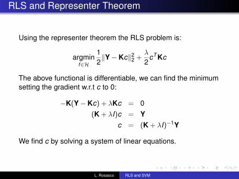
We derive the dual from the primal using the Lagrangian:
Cn∑
i=1
ξi +12
cT Kc −n∑
i=1
αi(yi{n∑
j=1
cjK (xi , xj)} − 1 + ξi)−n∑
i=1
ζiξi︸ ︷︷ ︸L(c,ξ,α,ζ)
Dual problem is:argmaxα,ζ≥0
infc,ξ
L(c, ξ, α, ζ)
First, minimize L w.r.t. (c, ξ):
(1) ∂L∂c = 0 =⇒ ci = αiyi
(2) ∂L∂ξi
= 0 =⇒ C − αi − ζi = 0=⇒ 0 ≤ αi ≤ C
L. Rosasco RLS and SVM
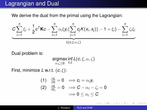
Lagrangian and Dual
We derive the dual from the primal using the Lagrangian:
Cn∑
i=1
ξi +12
cT Kc −n∑
i=1
αi(yi{n∑
j=1
cjK (xi , xj)} − 1 + ξi)−n∑
i=1
ζiξi︸ ︷︷ ︸L(c,ξ,α,ζ)
Dual problem is:argmaxα,ζ≥0
infc,ξ
L(c, ξ, α, ζ)
First, minimize L w.r.t. (c, ξ):
(1) ∂L∂c = 0 =⇒ ci = αiyi
(2) ∂L∂ξi
= 0 =⇒ C − αi − ζi = 0=⇒ 0 ≤ αi ≤ C
L. Rosasco RLS and SVM
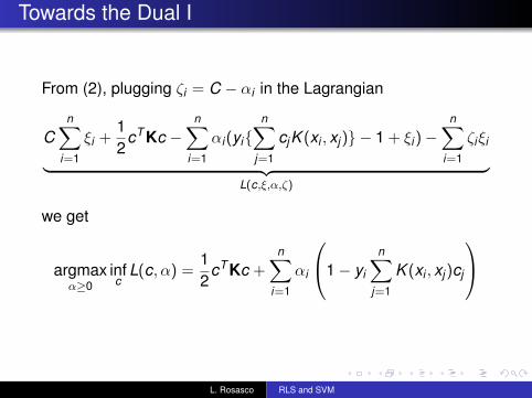
Towards the Dual I
From (2), plugging ζi = C − αi in the Lagrangian
Cn∑
i=1
ξi +12
cT Kc −n∑
i=1
αi(yi{n∑
j=1
cjK (xi , xj)} − 1 + ξi)−n∑
i=1
ζiξi︸ ︷︷ ︸L(c,ξ,α,ζ)
we get
argmaxα≥0
infc
L(c, α) =12
cT Kc +n∑
i=1
αi
1− yi
n∑j=1
K (xi , xj)cj
L. Rosasco RLS and SVM

Towards the Dual II
argmaxα≥0
infc
L(c, α) =12
cT Kc +n∑
i=1
αi
1− yi
n∑j=1
K (xi , xj)cj
Next plugging in (1), i.e. ci = αiyi , we get
argmaxα≥0
L(α) =∑n
i=1 αi − 12∑n
i,j=1 αiyiK (xi , xj)αjyj
=∑n
i=1 αi − 12α
T (diagY)K(diagY)α
L. Rosasco RLS and SVM

The Primal and Dual Problems Again
argminc∈Rn,ξ∈Rn
C∑n
i=1 ξi + 12cT Kc
subject to : ξi ≥ 1− yi(∑n
j=1 cjK (xi , xj)) i = 1, . . . ,nξi ≥ 0 i = 1, . . . ,n
maxα∈Rn
∑ni=1 αi − 1
2αT Qα
0 ≤ αi ≤ C i = 1, . . . ,n
The dual problem is easier to solve: simple box constraints.
L. Rosasco RLS and SVM

Support Vectors
The input input points with non zero coefficients are calledsupport vectors.We get a geometric interpretation using complementaryslackness, primal/dual constraints.
L. Rosasco RLS and SVM

Optimality Conditions
All optimal solutions must satisfy:
n∑j=1
cjK (xi , xj)−n∑
j=1
yiαjK (xi , xj) = 0 i = 1, . . . ,n
C − αi − ζi = 0 i = 1, . . . ,n
yi(n∑
j=1
yjαjK (xi , xj))− 1 + ξi ≥ 0 i = 1, . . . ,n
αi [yi(n∑
j=1
yjαjK (xi , xj))− 1 + ξi ] = 0 i = 1, . . . ,n
ζiξi = 0 i = 1, . . . ,nξi , αi , ζi ≥ 0 i = 1, . . . ,n
L. Rosasco RLS and SVM

Optimality Conditions
These optimality conditions are both necessary and sufficientfor optimality: (c, ξ, α, ζ) satisfy all of the conditions if and only ifthey are optimal for both the primal and the dual. (Also knownas the Karush-Kuhn-Tucker (KKT) conditons.)
L. Rosasco RLS and SVM

Interpreting the solution — sparsity
αi [yi(n∑
j=1
yjαjK (xi , xj))− 1 + ξi ] = 0, i = 1, . . . ,n.
Remember we defined f (x) =∑n
i=1 yiαiK (x , xi), so that
yi f (xi) > 1 ⇒ (1− yi f (xi)) < 0⇒ ξi 6= (1− yi f (xi))
⇒ αi = 0
L. Rosasco RLS and SVM

Interpreting the solution — support vectors
Consider
C − αi − ζi = 0 i = 1, . . . ,nζiξi = 0 i = 1, . . . ,n
yi f (xi) < 1 ⇒ (1− yi f (xi)) > 0⇒ ξi > 0⇒ ζi = 0⇒ αi = C
L. Rosasco RLS and SVM

Interpreting the solution — support vectors
Soyi f (xi) < 1⇒ αi = C.
Conversely, suppose αi = C. From
αi [yi(n∑
j=1
yjαjK (xi , xj))− 1 + ξi ] = 0, i = 1, . . . ,n.
we have
αi = C =⇒ ξi = 1− yi f (xi)
=⇒ yi f (xi) ≤ 1
L. Rosasco RLS and SVM

Interpreting the solution
Here are all of the derived conditions:
αi = 0 =⇒ yi f (xi) ≥ 10 < αi < C =⇒ yi f (xi) = 1
αi = C ⇐= yi f (xi) < 1
αi = 0 ⇐= yi f (xi) > 1αi = C =⇒ yi f (xi) ≤ 1
L. Rosasco RLS and SVM

Geometric Interpretation of Reduced OptimalityConditions
L. Rosasco RLS and SVM

The Geometric Approach
The “traditional” approach to describe SVM is to start with theconcepts of separating hyperplanes and margin. The theory isusually developed in a linear space, beginning with the idea ofa perceptron, a linear hyperplane that separates the positiveand the negative examples. Defining the margin as thedistance from the hyperplane to the nearest example, the basicobservation is that intuitively, we expect a hyperplane withlarger margin to generalize better than one with smaller margin.
L. Rosasco RLS and SVM

Large and Small Margin Hyperplanes
(a) (b)
L. Rosasco RLS and SVM

Maximal Margin Classification
Classification function:
f (x) = sign (w · x). (1)
w is a normal vector to the hyperplane separating the classes.We define the boundaries of the margin by 〈w , x〉 = ±1.
What happens as we change ‖w‖?
We push the margin in/out by rescaling w – the margin movesout with 1
‖w‖ . So maximizing the margin corresponds tominimizing ‖w‖.
L. Rosasco RLS and SVM

Maximal Margin Classification, Separable case
Separable means ∃w s.t. all points are beyond the margin, i.e.
yi〈w , xi〉 ≥ 1 , ∀i .
So we solve:
argminw
‖w‖2
s.t. yi〈w , xi〉 ≥ 1 , ∀i
L. Rosasco RLS and SVM

Maximal Margin Classification, Non-separable case
Non-separable means there are points on the wrong side of themargin, i.e.
∃i s.t. yi〈w , xi〉 < 1 .
We add slack variables to account for the wrongness:
argminξi ,w
∑ni=1 ξi + ‖w‖2
s.t. yi〈w , xi〉 ≥ 1− ξi , ∀i
L. Rosasco RLS and SVM

Historical Perspective
Historically, most developments begin with the geometric form,derived a dual program which was identical to the dual wederived above, and only then observed that the dual programrequired only dot products and that these dot products could bereplaced with a kernel function.
L. Rosasco RLS and SVM

More Historical Perspective
In the linearly separable case, we can also derive theseparating hyperplane as a vector parallel to the vectorconnecting the closest two points in the positive and negativeclasses, passing through the perpendicular bisector of thisvector. This was the “Method of Portraits”, derived by Vapnik inthe 1970’s, and recently rediscovered (with non-separableextensions) by Keerthi.
L. Rosasco RLS and SVM

Summary
The SVM is a Tikhonov regularization problem, with thehinge loss.Solving the SVM means solving a constrained quadraticprogram, rouhgly O(n3)
It’s better to work with the dual program.
Solutions can be sparse – few non-zero coefficients, thiscan have impact for memory and computationalrequirements.The non-zero coefficients correspond to points notclassified correctly enough – a.k.a. “support vectors.”There is alternative, geometric interpretation of the SVM,from the perspective of “maximizing the margin.”
L. Rosasco RLS and SVM

RLS and SVM Toolbox
GURLS (Grand Unified Regularized Least Squares)http://cbcl.mit.edu/gurls/
SVM Light: http://svmlight.joachims.orglibSVM:http://www.csie.ntu.edu.tw/~cjlin/libsvm/
L. Rosasco RLS and SVM