Embed Size (px)
Citation preview

OLIVIER JEAN BLANCHARD Massachusetts Institute of Technology
PETER DIAMOND Massachusetts Institute of Technology
The Beveridge Curve
OVER THE PAST thirty years, macroeconomists thinking about aggregate labor market dynamics have organized their thoughts around two rela- tions, the Phillips curve and the Beveridge curve. The Beveridge curve, the relation between unemployment and vacancies, has very much played second fiddle. We think that emphasis is wrong. The Beveridge relation comes conceptually first and contains essential information about the functioning of the labor market and the shocks that affect it.
Labor markets in the United States are characterized by huge gross flows. Close to seven million workers move either into or out of employment every month.1 While that movement could be consistent with workers reallocating themselves across a given set of jobs, recent evidence by Steve Davis and John Haltiwanger suggests that these flows are associated with high rates ofjob creation and job destruction. Using a measure of job turnover, defined as the sum of employment increases in new or expanding establishments and employment decreases in shrinking or dying establishments, Davis and Haltiwanger find that
We thank the National Science Foundation for financial assistance, Data Resources, Inc., for access-to their data base. We thank Hugh Courtney and Juan Jimeno for excellent research assistance; John Abowd and Arnold Zellner for their gross flow data; Katharine Abraham for help with the vacancy data; Roger Gordon, Nils Gottfries, Jerry Hausman, Larry Katz, David Lilien, Chris Pissarides, Bob Solow, Larry Summers, members of the Brookings Panel, and our discussants for comments.
1. Information on gross flows of workers comes from the monthly Current Population Survey. It is well known that measurement error leads to an upward bias in the raw data on gross flows, and various adjustments have been suggested to remove the bias. The number in the text refers to the gross flows as adjusted by Abowd and Zellner (1985). Poterba and Summers (1986), using a different method of adjustment, obtain an estimate of those flows equal to only 60 percent of the Abowd-Zellner estimate.
1

2 Brookings Papers on Economic Activity, 1:1989
during 1979-83, a period of shrinking employment, job turnover in manufacturing averaged some 10 percent per quarter.2 From a macro- economic viewpoint, the labor market is highly effective in matching workers and jobs, yet those flows are so large that they imply the coexistence of unfilled jobs and unemployed workers. Examination of the joint movement of unemployment and vacancies can tell us a great deal about the effectiveness of the matching process, as well as about the nature of shocks affecting the labor market. In this paper, we first develop a conceptual frame in which to think about gross flows, about the matching process, and about the effects of shocks on unemployment and vacancies. We then turn to the empirical evidence, using data for the postwar United States. We focus first on the matching process, estimating the "matching function," the aggregate relation between unemployment, vacancies, and new hires. We then interpret the Bev- eridge relation. More precisely, we look at the joint behavior of unem- ployment, employment, and vacancies, and infer from it the sources and the dynamic effects of the shocks that have affected the labor market over the past 35 years.
Our conceptual starting place is a minimalist model describing the gross flows of both workers and jobs. We think of an economy in which, at any instant, many jobs become profitable and many jobs become unprofitable. To find workers for those newly profitable jobs, firms post vacancies. Workers in jobs that become unprofitable are laid off and look for newjobs. The complex process through which workers and jobs look for and find each other is represented by a simple aggregate matching function, giving new matches as a function of both unemployment and vacancies. At given rates of job creation and destruction, the economy would settle to a steady level of unemployment and vacancies, deter- mined by both the rates of job creation and destruction and the effec- tiveness of the matching process. The economy, however, is subject to two types of shocks with quite different effects. Changes in the level of aggregate activity cause rates ofjob creation and job destruction to move in opposite directions, while changes in the intensity of the reallocation process cause them to move in parallel. The dynamic effects of those two types of shocks on unemployment and vacancies follow easily. Aggregate activity shocks drive unemployment and vacancies in oppo-
2. Davis and Haltiwanger (1989).

Olivier Jean Blanchard and Peter Diamond 3
site directions, causing counterclockwise movements around a down- ward-sloping locus in the Beveridge space. Reallocation shocks lead instead to movements along an upward-sloping locus, to parallel move- ments in unemployment and vacancies. The model therefore provides a way of looking at the Beveridge relation and tells us what can be inferred from the actual comovements of unemployment and vacancies.
To focus on the basic mechanisms, the initial model ignores important features of actual labor markets. It assumes an exogenous labor force, an exogenous stock of potential jobs, that only the unemployed getjobs, that quit rates are constant, and that all unemployed workers are identical. Even a cursory glance at the data shows all these assumptions to be wildly incorrect. Much of the movement into and out of employment is from "out of the labor force," many workers move from one job to another without experiencing unemployment, the quit rate is highly procyclical, and many of the unemployed remain attached to, and return to, the firms that have laid them off. To take the data into account, we extend the model to allow for some of those features. Throughout, our emphasis remains on the effects of shocks on the aggregate labor market variables. The picture we get is richer than, but fundamentally similar to that obtained in the initial model.
Critical to our thinking about labor markets is the notion of a matching function. This function hides a complex reality in which geographic and skill differences between workers and jobs, as well as the intensity of search on the part of workers and firms, all matter. One may legitimately wonder whether such a function exists at all. We thus start our empirical investigation by looking for that function. To do so, we make use of the gross flow series as adjusted by John Abowd and Arnold Zellner and of the help-wanted index as a proxy for vacancies as adjusted by Katharine Abraham.3 Because adjusted flow series begin in 1968, and manufactur- ing flow series, which we need in the construction of new hires, end in 1981, 1968-81 becomes the sample period. For that period, we find a strong, stable relation between aggregate new hires, unemployment, and vacancies. The relation is well approximated by a Cobb-Douglas function, with constant or mildly increasing returns, and relative coeffi- cients of 0.4 on unemployment and 0.6 on vacancies. The estimates imply that the average duration of vacancies varies from two to four
3. Abowd and Zellner (1985); Abraham (1987).
4 Brookings Papers on Economic Activity, 1:1989
weeks depending on labor market conditions and thus show two impor- tant aspects of the labor market. From a macroeconomic point of view, matching is highly effective: firms and workers easily achieve matches. Firms' ability to find workers, however, depends on the state of the labor market: employment is not simply determined by demand. Study- ing the function in more detail reveals four more things. First, somewhat to our surprise, even when unemployment becomes very large, its marginal effect on new hires does not disappear. Second, the relevant pool of workers appears to include some workers classified as being out of the labor force. Third, the long-term unemployed contribute as much to aggregate new hiring as do the short-term unemployed. Finally, across all specifications, we consistently find a negative time trend, implying a decline in the hiring rate at given levels of the vacancy and unemployment rates.
Next we turn to the data on unemployment, the labor force, and vacancies (again proxied by an adjusted help-wanted index). Our earlier analysis suggests that we should think of their dynamics as coming from the dynamic effects of aggregate activity, reallocation, and labor supply shocks (exogenous movements in the labor force). We estimate the joint process generating those three variables and, using a set of just-identi- fying assumptions, recover both the shocks, or, more precisely, the innovations to those shocks, and their dynamic effects. We are thus able to decompose the history of joint movements in the unemployment and the vacancy rate, the Beveridge curve, into movements due to each of the three shocks. Looking at those movements on a month-by-month basis, we find that aggregate activity shocks dominate, with effects similar to those characterized in our model. Except at low frequencies, reallocation and labor force shocks contribute little to the fluctuations in the unemployment or the vacancy rate. Both findings are important. In particular, that reallocation shocks do not appear to explain much of the fluctuations in unemployment confirms the findings of Katharine Abraham and Lawrence Katz in the debate on the macroeconomic importance of "sectoral shocks. " 4 The picture is different when we look at low frequencies. Roughly half the shift to the right of the Beveridge relation over the postwar period is due to the long-run effects of reallocation shocks. The other half is due to an unexplained deterministic
4. Abraham and Katz (1986).

Olivier Jean Blanchard and Peter Diamond 5
trend. While this trend could come from trends either in the underlying shocks or in the structure in the economy, the nature of the movement and our earlier finding of a drift in the matching function point to that drift as a major proximate cause of the shift of the Beveridge curve.
Throughout, our paper ignores wage determination. The formal justification in our model is the assumption that wages play no allocational role in individual matches, merely dividing rents between firms and workers. The real reason we ignore wage determination, however, is our desire to concentrate first on the Beveridge relation and to leave other issues to later. But it is clear that, whether or not it is extended to allow for wages to play an allocational role, our approach yields a theory of the joint behavior of unemployment, vacancies, and wages. Put crudely, it allows for an integration of the Phillips curve and the Beveridge curve. That vacancies are a strong determinant of wages, stronger than unemployment in many countries, has long been documented. That shifts in the Beveridge curve may shed light on Phillips curve movements has also long been recognized. In the conclusion to this paper, we review our main results and give a brief preview of how our approach may shed light on those issues.
A Minimalist Model of Vacancies and Unemployment
The purpose of our initial model is to capture the two elements we see as essential to any description of labor markets. The first is that, at any particular time, even during the worst recessions, many firms want to increase their labor force and many firms want to decrease theirs. The second is that there is no centralized allocation mechanism; firms who want new workers, and workers who want jobs, must locate each other. To concentrate on the basic implications of those two elements, we leave out most of what makes the texture of actual labor markets.' We return to some of those missing aspects in the next section.
5. Ours is not the first model of unemployment and vacancies. We build on the early work of Holt and David (1966); Phelps (1968); and Hansen (1970). Our model has, however, more in common with Pissarides (1985). Our model leaves out many of the effects Pissarides concentrates on; it is, as a result, much simpler and can be used to study richer dynamic issues. There is one substantive difference between the two models in the treatment of vacancies, to which we point later.

6 Brookings Papers on Economic Activity, 1:1989
Workers and Jobs
We think of the economy as being composed of identical workers and jobs. Workers can be employed, unemployed, or out of the labor force. In actual labor markets, the difference between the unemployed and those out of the labor force is one of degree. In our model, the difference is a sharp one. The unemployed look for work; those out of the labor force do not. Let E be the number of employed workers, U the unemployed, and N the workers not in the labor force. In the initial model, we take the number in the labor force, L, as given. The first relevant equation is therefore
(1) L=E+ U.
Symmetrically, jobs can be filled, unfilled with a vacancy posted ("vacancies" for short), or unfilled with no vacancy posted ("idle capacity"). Each job requires one worker. Again, we draw a sharper distinction between unfilled jobs with or without a vacancy posted than is true of actual labor markets: only firms with jobs for which a vacancy is posted are looking for workers. Let K be the total number of jobs, F the filled jobs, V the vacancies, and I the idle jobs, those that are unfilled with no vacancy posted. Thus,
(2) K=F+ V+I.
Obviously F and E are equal. In our initial model, we take K as given. Note that, by taking K and L to be constant, we treat the two sides of the market in asymmetric fashion. The reason will be clear below: our focus here is on shocks to the supply of jobs, not on shocks that affect whether workers decide to enter or drop out of the labor force.
Job Creation and Job Destruction
In the U.S. economy, jobs are always being created and terminated. They are created both in existing firms and through the appearance of new firms. They are terminated both in existing firms and, more drasti- cally, through closures and bankruptcies. Jobs may disappear forever or temporarily. We capture this process of creation and destruction through the following assumptions.
We think of each of the Kjobs in the economy as producing, if filled, a gross (of wages) revenue of either 1 or 0. Profitability for each job

Olivier Jean Blanchard and Peter Diamond 7
follows a Markov process in continuous time. A productivejob becomes unproductive with flow probability r0.6 An unproductive job becomes productive with flow probability ulr. Thus, the times to a change in profitability are Poisson processes. At any time, some jobs become productive, somejobs become unproductive. Whether newly productive jobs are jobs that were previously unproductive, or simply new jobs, is purely a matter of interpretation. This is the mechanism we use to generate the existing large gross flows ofjob creation andjob destruction. By making this process mechanistic (not dependent on underlying decisions) we have a simpler (albeit less accurate) setting for focusing on the complexity of aggregate dynamics.
The parameters 'ro and u I play a central role below. It is, however, more intuitive to think of two other parameters, c and s, which are defined from 'ro and wlr. For given 'ro and wlr, the proportion of potential jobs that are productive in steady state is given bywr 1,/Qro + wlr); we may think of this proportion, which we shall call c (for cycle), as measuring the degree of aggregate activity (or, more precisely, potential aggregate activity, as the proportion of jobs productive and filled will always be less than c). In steady state, the instantaneous flow of jobs changing from productive to unproductive (which equals the reverse flow) is equal to r0'r11/(Qr0 + ulr) times K; we can think of this ratio, which we shall denote s (for shift), as an index of the intensity of reallocation in the economy.
The Matching Process
If vacant jobs were instantaneously filled, the economy would have employment equal to cK. Changes in s, the intensity of the reallocation process, would not affect aggregate employment. But the process of matching workers and jobs is not instantaneous.
We envision each worker and firm as engaged in a time-consuming (stochastic) process of waiting for and looking for an appropriate match. We formalize this matching process by a matching function, giving new hires h as a function of unemployment and vacancies:
(3) h = ox m(U, V),
where ot is a scale parameter, and mu, my ' 0, m(0, V) = m (U, 0) = 0.
6. That is, in any short interval of time At there is a probability 'orAt of the job becoming unprofitable.

8 Brookings Papers on Economic Activity, 1:1989
This matching function is analogous to an aggregate production function. It recognizes that the large labor market flows generate delays in the finding of both jobs and workers even though the process is extremely efficient. It is simply not infinitely efficient.
This function is consistent with the idea that new jobs and workers differ in their geographic and skill characteristics, that, for example, the regions with high rates of job creation may not be those with high rates of job destruction. Changes in the parameter ot are intended to capture such changes in geographic or other differences between jobs and workers-what is sometimes called mismatch-as well as differences in search behavior.7
This function implies the simultaneous coexistence of unemployment and vacancies. An alternative formalization of the Beveridge relation, which we find less attractive, relies on aggregation of separate markets, each of which has no friction, with the outcome in each separate market being either unemployed workers or unfilled vacancies. This is the approach initially followed by Bent Hansen in the first formal model of the Beveridge curve, and more recently by a number of European researchers working on disequilibrium models.8
The Equations of Motion
To complete the specification of the model, we make one final assumption, namely that job terminations are not the only source of separations, but that workers quit jobs at an exogenous, constant rate, q. We introduce quits partly for the sake of-some-realism, but also because there is a basic distinction between quits and job terminations in the model. A quit is associated with the posting of a new vacancy; a job termination is not. Here again, the distinction is sharper in the model than in actual labor markets, where quits are often used by firms to reduce their labor force and are not always replaced. The assumptions that the quit rate is constant and that all quits are to unemployment are both counterfactual, but not central to the issues at hand.9
7. For one among many discussions of the matching function in the search literature, see Howitt and McAfee (1987). An important question, on which we shall not concentrate here, but to which we return in our empirical work below, is that of the degree of returns to scale of m.
8. Hansen (1970); Dreze (1989) and references therein. 9. It is straightforward to extend the analysis to allow the quit rate to be, for example,
a function of unemployment, or of unemployment and vacancies.

Olivier Jean Blanchard and Peter Diamond 9
It follows from our assumptions that the behavior of the labor market is given by a system of two differential equations:
(4) dEldt = otm(U, V) - qE - uDE,
(5) dVldt = -otm(U, V) + qE + w1TI - woV.
We consider these equations in turn, starting with the behavior of employment.
When ajob becomes unproductive, there is no reason for the worker to remain on thejob. 10 Thus, the flow from employment to unemployment from this source is equal to rrDE. In addition, the flow of quits is equal to qE. The flow from unemployment to employment is equal to new hires.
For ajob to produce 1, it must be not only productive but also matched with a worker. To do so, a vacancy must be posted and a worker must be recruited. There are thus two sources of new vacancies. The first source, a flow from Ito V, is unproductive jobs that become productive; this first flow is equal to wjrI.1" The second source, from F to V, is the need to replace workers who quit; it is equal to qE. Vacancies decrease for two reasons; some are filled by new hires, a flow from V to F. Some of the jobs for which vacancies were posted become unproductive, a flow from V to I; we assume that vacancies become unproductive at the same rate as filled jobs.
Using the identities above, we can rewrite these equations as a system in unemployment and vacancies, given K and L:
(6) dUldt = -onm(U, V) + (q + To))(L - U),
(7) dVldt = -otm(U, V) + (q - T1) (L - U) + 7TK - (o + 7T1) V.
10. We commit a theoretical sleight of hand here. If the probability that thejob becomes productive again is high enough, it may pay the firm and the worker to stay together. While the current surplus is equal to zero, the firm does not have to post a vacancy and wait for a new worker when the job turns productive again. We assume that the probability 'ai is low enough that this problem does not arise.
11. This is where we differ in an important way from Pissarides (1985). Pissarides assumes that firms create vacancies until the value of a new vacancy is equal to zero. We assume instead that, at any time, the number of potential vacancies, which depends on the number of jobs that are potentially productive, is very much given to firms. These alternative assumptions lead to substantive differences in the characterization of the joint movements of unemployment and vacancies. We feel that having the value of a vacancy equal to zero is an appropriate long-run restriction, but is not appropriate in the short run; see Diamond (1981).

10 Brookings Papers on Economic Activity, 1:1989
This account of the labor reallocation process has not mentioned wages. Wages are likely to affect K and L as well as c and s. But we take K, L, c, and s as given in this model. Wages could also affect whether a meeting between a worker and a firm actually leads to a hiring, thus affecting m or ox. We assume that they do not affect matching. That is, we consider a situation where first the worker and the firm examine whether there is a mutually advantageous opportunity to begin an employment relationship. If there is, they then negotiate a wage to divide the surplus from the match with no constraint (for example, fairness, union contracts, or posted wages) on allowable bargains. In a richer model with heterogeneous workers, jobs, and matches, the nature of bargaining power between the two sides would still affect allocation by affecting expectations about future opportunities. We shall ignore such complications, explicitly assuming homogeneous workers and firms, or absorbing the implications of heterogeneity into the parameters of the model. In this way, we can focus on the labor force, unemployment, and vacancies, ignoring wage and price dynamics. Of course, this ignores important effects of fairness constraints on wages paid to different employees of the same firm, and the effects of wages set ahead of time on a take it or leave it basis by firms or in union contracts. These are aspects left for later work.
Steady State and Dynamics
Setting dUldt and dVldt to zero, we have the steady-state values of V and U satisfying
(8) otm(U, V) = (q + wTo)(L - U),
(9) ot m(U, V) = (q - Tl) (L - U) + T1K - (wo + wl) V.
Figure 1 shows the two stationary curves, where dUldt and dVldt are each zero, as well as the directions of movement that satisfy the differential equations 6 and 7. The relevant region of the plane has U, V, E, and I all nonnegative. The locus dUldt = 0 is downward sloping. It does not hit the V axis given that m is equal to zero if V is equal to zero. The dVldt = 0 locus need not be monotonic. Nevertheless there is a unique, stable equilibrium, which is always a node.
To think of the dynamics of U and V, we have to specify the source of shocks to the economy. It is natural to think of changes in 'ro and wrr

Olivier Jean Blanchard and Peter Diamond 11
Figure 1. Directions of Motion
V
K-L
Vo
U~~~~~~~ 0 L
as the important source of fluctuations in the system. But looking at changes in one wr keeping the other constant does not appear to be a particularly relevant experiment. We find it more attractive to think in terms of two types of shocks-shocks that affect aggregate activity while leaving the degree of reallocation constant and shocks that affect the degree of reallocation keeping aggregate activity constant. Using our earlier definitions of c and s, the first is a shock to c, leaving s constant; the second is a shock to s, keeping c constant. Since Tro = slc and TrI =
sl(l - c), we can rewrite the dynamic system in terms of s and c:
(10) dUldt = -otm(U, V) + [q + (slc)](L - U),
(I1) dVldt = -otm(U, V) + q(L - U)
+ [sl(l - c)] (K- V-L + U) - (slc)V.
We consider first the effects of a once and for all change in s, the intensity of reallocation. The change in the steady-state values of U and

12 Brookings Papers on Economic Activity, 1:1989
V is easily characterized by noticing that setting dUldt = 0 and dVldt =
O in equations 10 and 11 and eliminating s from the two equations gives
(12) (L-U) = cK-V.
Thus, the locus of steady states for different values of s and a given value of c lies along a 45 degree line.
In addition to characterizing steady states, it is easy to describe the dynamic path from a change in s when the economy starts at a steady- state point (that is, satisfies equation 12). Evaluating dUldt and dVldt at a point satisfying equation 12, we have
(13) dVldt = -otm(U, V) + [q + (sic)] (cK - V) = dUldt.
Thus, if the economy is subject only to s shocks, to changes in reallocation intensity, it will move up and down a 45 degree line. 12 The same is true of shifts in ox, the parameter of the matching function, which captures another dimension of mismatch. Like changes in s, changes in cx leave equation 12 unchanged, and thus also move the steady state-and movements from the steady state-along the same 45 degree line. Figure 2 gives the dynamic effects of once and for all changes in ox or s on unemployment and vacancies.
Similarly analyzing changes in c, aggregate activity shocks, we first calculate the locus of steady states for a given s and varying c. This is done by eliminating c from the steady-state versions of equations 10 and 11, to get the locus
(14) (L - U + V) [otm(U, V) - q(L -- U)] = sK(L - U),
which is downward sloping. This locus, the steady-state relation between U and V for different levels of aggregate activity, is often what econ- omists have in mind when they refer to the Beveridge curve. But it is only a steady-state locus. The existing literature discusses counterclock- wise movements around the steady-state locus.13 We find indeed that, in response to changes in c, the economy is likely to produce counterclock- wise loops around the steady-state locus.14 Figure 3 gives the dynamic
12. For an economy experiencing both c and s shocks, the response to s shocks is not this simple. The slope of the actual path after an s shock depends on the initial position, as is clear from the phase diagram in figure 1.
13. For example, Hansen (1970). 14. The proof and exact conditions are as follows. We first examine the slope of a

Olivier Jean Blanchard and Peter Diamond 13
Figure 2. Shift in Reallocation Intensity (s)
V
K - -- -- -- -- -- -- -- ---_-_-_-_-
K-L Dynamic
path
(s1) =O0
V (sV ) = 0
0 L
trajectory through some point on equation 14. Each point on equation 14 is associated with some value of c, each trajectory is associated with another value which we denote by c'. From equations 10 and 11, we have
dV/dU = (dV/dt)/(dU/dt) = {-m + q(L - U) + [s/(1 - c')] (K- V+ L + U) - (sc')V}I/
um + q(L - U) + (slc')(L - U)]. The issue is whether the above equation, evaluated at a point on equation 14, exceeds the slope of the locus at that point, which from equation 14 is given by
dV/dU= - {[V/(L - U )] [m - q(L - U )] + (L - U + V)(mnu + q)}/
[oam - q(L - U ) + (L - U+ V)otmv]. The term (dV/dU) in the first equation is decreasing in c'. As c' goes to one, it goes to minus infinity. Thus, the interesting question is that of what happens as c' goes to zero. When c' = 0, the first equation equals - V/(L - U ). Comparing - V/(L - U ) to the second equation shows that paths are always counterclockwise if and only if
Va.m v > (L - U )(in u + q)- Assuming that m has constant returns to scale, this is equivalent to
am(U,V)>Lcamu + (L-U)q.
Since am > (L - U )q from equation 14, this condition will hold as long as umu is not too large, or equivalently as long as amv is not too small.

14 Brookings Papers on Economic Activity, 1:1989
Figure 3. Shift in Aggregate Activity (c)
V
K-
K-L) = \ \(ce) = 0 K-L X
Dynamic V(c1)=O ~~~path
V (c0) =O
Beveridge curve
0 L
effects of a once and for all increase in c on unemployment and vacancies. To summarize, the high rates of job creation and destruction explain
the coexistence of unemployment and vacancies. Decreases in aggregate activity lead to increases in unemployment and decreases in vacancies. Increases in the intensity of reallocation also increase unemployment but increase vacancies as well. The model clearly shows that high unemployment can be due either to aggregate activity factors or to structural changes requiring the reallocation of labor, and that looking at both unemployment and vacancies can shed light on the sources of unemployment movements. Before we can do so, however, we must take up a number of issues brushed aside in this section.
Extending the Model
Our initial model is built on many counterfactual assumptions. Some can be relaxed at some cost in simplicity, but without changing the

Olivier Jean Blanchard and Peter Diamond 15
general picture much. Some, however, need to be modified before we can take the model to the data. 15
The first is the sharp distinction drawn in the model between those out of the labor force and those unemployed. Differences between those two pools are in fact fuzzy. The flows between the two are large and respond to economic activity. And new hires do not come only from the ranks of the unemployed. As computations presented in the next section show, roughly 45 percent of hires come from unemployment, 40 percent from out of the labor force, and 15 percent from employment, from workers moving directly from one job to another.
The second assumption to be moditied is that the pool of workers available for hire is homogeneous. Workers out of the labor force but available for work are unlikely to behave exactly as those unemployed. Even within the unemployed, some are more actively searching than others. Some keep a close attachment to a firm and can simply be called back by firms; others are unattached. Many laid off workers in manufac- turing are eventually recalled, a phenomenon, first emphasized by Martin Feldstein, that is quite different from the picture of the labor market sketched above. 16
We thus consider two extensions of our model. The first allows for both exogenous and endogenous movements in the labor force, focusing on the entry of workers in the labor force in response to changes in employment, rather than on the direct hiring from out of the labor force. This extension is little more than the straightest short cut, useful mainly to point out basic differences and to organize the empirical work later. The second extension explores the idea that the relevant pool of workers is heterogeneous with respect to matching. We focus on the distinction between attached and unattached workers.
Labor Force, Unemployment, and Vacancies
Steady increases in the labor force, such as the entry of new cohorts, trend changes in participation, and so on, are likely to be associated with
15. A description of the various flows in the labor market, of the decisions associated with those flows, and of their implications for the relation between vacancies and unemployment in the labor market was developed by Holt and David (1966) in one of the early papers on the Beveridge curve.
16. Feldstein (1975).

16 Brookings Papers on Economic Activity, 1:1989
steady increases in capital accumulation and creation of new jobs. Modifying the initial model to allow for steady growth of both K and L is straightforward. Assume that K and L grow at the same rate n and assume constant returns in matching. Assume that all new workers start unemployed and all new jobs come on line profitable. Define u = UIL, v = V/L, and k = KIL. Then the equations of motion become
(6') duldt= - otm(u, v) + (q + TrO + n) (1 - u),
(7') dvldt = -otm(u, v) + (q - l1)(1 - u) + (m, + n)k
- (r0 + a, + n)v.
The analysis then proceeds very much as before, with the implication that the growing labor force is steadily matched with new jobs. Neither steady-state u nor steady-state v is necessarily monotonic in n.
We want, however, also to focus on movements in the labor force that are not accompanied by simultaneous increases in capital, or movements that occur in reaction to movements in labor market condi- tions. A simple formalization is
(15) dLldt = a(dEldt) + f, I > a > O.
Labor force movements depend on an exogenous component, f, and on movements in employment: an increase in employment leads some workers tojoin the labor force, increases participation, while a decrease leads some to leave. The focus here is on the movements between unemployment and out of the labor force; the analysis of the movements directly between out of the labor force and employment is better done in a model with two pools along the lines of the model in the next subsection. The specification embodied in equation 15 is obviously rough. Decisions to enter or leave the labor force must in part depend on wage determination: how the surplus from a match is divided between firms and workers will affect the decision of workers to stay, exit, or enter the labor force. For the same reason, those decisions are likely to depend on both vacancies and unemployment, rather than just on employment.
Maintaining the assumption that all hires still come from the ranks of

Olivier Jean Blanchard and Peter Diamond 17
the unemployed, using equations 10, 11, and 15, and using the definitions of s and c gives us a system in L, V, and U:
dLldt = - [aI(l - a)] (dUldt) + [1/(1 - a)]f,
(16) dVldt = -onm(U, V) + q(L - U) + [s(l - c)] (K - V - L + U)
- (slc)V,
dUldt = -(1 - a)o-m(U,V) + (1 - a)[q + (slc)](L - U) + f.
In this extended model, shocks now affect vacancies, unemployment, and the labor force. And there are now three rather than two sources of shocks: aggregate activity, reallocation, and labor supply shocks, c, s, andf, respectively.
The effects of aggregate activity and reallocation shocks are little changed, except for the positive comovements of the labor force with employment. The dynamic effects of c and s can be derived by noting that, iff is equal to zero, one can define L* U + (1 - a)E = (1- a)L + a U, which is constant. Substituting L* in the last two equations gives a system of two differential equations in U and V. The dynamics of this system with respect to either c or s shocks are similar to those charac- terized earlier, although differing in detail.
To see the effects of labor supply shocks, it is easiest to consider a discrete change in L, rather than the more complex change infin equa- tion 15. Assuming further that a = 0 and that q = sI(1 - c) makes the analysis easy to carry out and is not misleading. The dynamic effects of an increase in L are drawn in figure 4. In that case, the (dVldt = 0) curve does not shift and the (dUldt = 0) locus shifts up. An increase in the labor force thus leads to an increase in unemployment that is less than one for one, and to a decrease in vacancies. The instantaneous effect of the labor force increase is to increase unemployment one for one, and, as higher unemployment leads to a higher rate of hire, to increased matching. Then, over time, unemployment decreases and so do vacan- cies. This decrease in unemployment represents a higher level of utilization of the capital stock; if we were to allow for a response of capital accumulation, these newjobs would further decrease unemploy- ment. One might think of the economy as satisfying equation 16 in the short run but satisfying equations 6' and 7' in the long run.

18 Brookings Papers on Economic Activity, 1:1989
Figure 4. Labor Force Shock (f)
V
K |- -- -- -- ---- - - - - - -
K-L/
L(f) = 0
K-LI Dynamic path
X ~~~V= 0
U(f0)O)= \ U(~~~~~~~~
0 Lo LI
Attached and Unattached Workers
In thinking about heterogeneity of the pool of workers, we have chosen to explore one dimension that seems particularly important for short-run dynamics-the distinction between attached and unattached workers. A worker who is laid off may remain attached to the firm in two distinct senses. One is that the worker is less available for employ- ment elsewhere than the typical unemployed worker. The second is that the worker is available for recall by the firm without the need to post a vacancy. This practice is most common in manufacturing.
We formalize attachment as follows. We assume that a fraction g of all workers who are laid off remain initially attached to their job. In this way, we draw a distinction between the recycling of particular jobs in successions of bad and good shocks, and a birth and death process in which some jobs are replaced by others. The remaining fraction of laid off workers (1 - g) is unattached. Over time, if not recalled or hired in

Olivier Jean Blanchard and Peter Diamond 19
another job, the attached workers steadily drift away, becoming part of the pool of unattached unemployed.
Denote by Ua and Un the pool of attached and unattached workers, respectively. Leaving recalls aside, hiring can come from both pools, although perhaps under different conditions: attached workers may be searching less or be more selective in their choices. The two hiring functions are denoted ma(Ua, Un, V) and m,(Ua, Un, V). The rate at which attached workers become unattached is assumed, for conven- ience, to be the same as the quit rate from employment. Workers who quit become unattached upon quitting. The equations of motion are then given by
dUaldt = -ma-i7Ua-qUa + g7o(L-Ua-Un),
dUnldt = -mn + q(L - Un) + (1 - g)To (L - Ua- Un)
dVldt = -ma - M,l + q(L - Ua - Un) -T, (L - Uj)
+ aIK - (so + Tr)V.
The number of attached workers shrinks from new hires, recalls, and breakup of attachment; it increases as a result of layoffs. The number of unattached workers shrinks from new hires and increases as a result of permanent layoffs, breakups of attachment, and quits from employment. Finally the vacancy equation differs from that of the previous section by the absence of a, Ua, since those good shocks result in a recall rather than in the posting of a vacancy.
How will the dynamics of this extended model differ from those of the minimalist model? We shy away from a full analysis here but point to a number of important differences.
In an economy in which workers remain highly attached to firms, much of the movement into and out of unemployment will take place without vacancies being posted, as firms will have a pool of workers from which to rehire. More generally, what happens to vacancies and unemployment after a shock will depend on the initial stocks of attached and unattached workers, which themselves will depend on the history of the shocks. After a sharp but short-lived contraction, firms will be able to increase employment without relying much on vacancies. After a protracted recession, the pool of attached workers may have shrunk enough to force firms to increase employment mostly through new hiring.

20 Brookings Papers on Economic Activity, 1:1989
Whether aggregate activity shocks generate counterclockwise move- ments in the Beveridge space is much more ambiguous. An increase in c leads firms to recall a number of workers as well as to post new vacancies. Thus, in contrast to the initial model where increases in vacancies are likely to lead decreases in unemployment, unemployment may now decrease initially as fast as or faster than vacancies increase.
This model suggests constructing proxies for the pools of attached and unattached workers and looking at the joint behavior of those two pools and vacancies together, a suggestion we shall not follow in this paper. At the very least, however, it alerts us to the potential relevance of attached worker unemployment, something we shall take into account in the empirical work below. We end the presentation of this model with two remarks.
We would expect g, the proportion of attached workers, to vary with s. One reason is that jobs created by reallocation shocks are more likely to be genuinely new opportunities and therefore less likely to have attached workers. Another is that attachment is likely to depend on the prospects of thejob reopening; workers are less likely to remain attached to jobs that disappear permanently. This opens another avenue for distinguishing empirically between aggregate activity and reallocation shocks.
One can think of other potentially relevant distinctions between groups of workers for which a similar framework can be used. One is the distinction between those hired from the ranks of the unemployed and those hired from out of the labor force; it is reasonable to assume that the hiring functions differ between the two groups. Another is between the short- and the long-term unemployed: the issue of whether, control- ling for heterogeneity, the long-term unemployed are less likely to be hired is an old one in labor economics. Our empirical evidence in the next section suggests, however, that it may not be an important distinc- tion from a macroeconomic point of view.
The Matching Function
Our conceptual model makes heavy use of an aggregate matching function, the function that relates the flow of new hires to the stocks of vacancies and unemployment. Like the aggregate production function,

Olivier Jean Blanchard and Peter Diamond 21
the aggregate matching function is an abstract but convenient device, which partially captures a complex reality. In this case, the reality is one of workers looking for the right job, ofjobs looking for the right worker, all with varying degrees of intensity and success. Changes in the nature of new jobs, in the location of job creation and job destruction, and in the search behavior of the unemployed will all shift this function. In this section, we look for such a function in the data and we find it. 17 We find that there is indeed a strong, stable relation between new hires and both unemployment and vacancies. We draw the implications of our findings as we go along.
New Hires, Vacancies, and Unemployment
As we have emphasized, the labor market is highly effective in allocating workers to jobs: the flows are large in proportion to stocks; the average duration of unemployment rarely exceeds three months; the average duration of vacancies does not exceed a month. We therefore estimate the matching function using the highest-frequency observations available, namely monthly data. None of the series needed to estimate the matching function is directly available. We construct the three series as follows (specific sources and details of construction are given in appendix A).
We construct new hires as the sum of the flows into employment from unemployment and from out of the labor force, to which we add the estimated flow from employment to employment, and from which we subtract the estimated flow of workers who are recalled rather than newly hired.
The flows into employment from unemployment and from out of the labor force are available monthly from the Current Population Survey.'8
17. Pissarides (1986) estimates a matching function for the United Kingdom, with less success. We have not examined why the two sets of results differ. Our specifications are different. Despite the amount of data construction, our data coverage is broader and our data are probably better. But the histories of unemployment in the United Kingdom and the United States over the past 15 years differ substantially; the matching function may not be invariant to the history of unemployment.
18. More precisely, these flows give the number of workers in state i in the previous month and statej in the current month. A worker who went from out of the labor force to unemployment to employment within a month would be counted as having moved from out of the labor force to employment.
22 Brookings Papers on Economic Activity, 1:1989
As is well known, the reported gross flows are biased upward, as incorrect classification of workers generates spurious transitions and thus in- creases measured gross flows. Both Abowd and Zellner, and Poterba and Summers have developed techniques to remove the bias in the raw series. '9 We use the gross flow series as adjusted by Abowd and Zellner, which are available from the beginning of 1968 through May of 1986. They imply, for that period, average monthly flows of 1.5 million workers from unemployment to employment and 1.4 million workers from out of the labor force to employment.20
To those two flows, we must add the flow from employment to employment, the number of workers who quit a job for another. This flow has been the focus of a recent paper by George Akerlof, Andrew Rose, and Janet Yellen, who review the available evidence.21 They conclude that employment-to-employment quits account for roughly 40 percent of all quits. There is little available evidence about the time series behavior of that proportion. To construct a series, we assume that the proportion of such quits is constant and equal to 0.4, and that quit behavior depends on overall labor market conditions so that the quit rate for the economy as a whole is the same as the quit rate in manufacturing. The manufacturing quit rate series is available through 1981, after which it was discontinued. This and the starting date of adjusted gross flow data determine the period of estimation below, from the beginning of 1968 through the end of 1981. The employment-to-employment flow series so constructed is highly procyclical and is on average equal to half the flow from unemployment to employment. We investigate below the robustness of our findings to changes in the construction of the employ- ment-to-employment quits series.
19. Abowd and Zellner (1985); Poterba and Summers (1986). 20. The Poterba and Summers adjustments yield a fairly different picture of both the
absolute and relative sizes of these flows. For the period 1977-82-for which a comparison can be made-the raw gross flows from unemployment and out of the labor force to employment are 1.8 million and 2.8 million, respectively. The Abowd-Zellner correspond- ing flows are 1.8 million and 1.4 million, respectively. The Poterba-Summers corresponding flows are 1.4 million and 0.4 million only. While these differences between adjusted series are disturbing, we guess that to the extent to which both adjustments are mostly adjustments of the levels, the two sets of series are likely to have roughly the same time series properties. (This is a guess, as the Poterba-Summers adjusted series do not exist for the period we are interested in.)
21. Akerlof, Rose, and Yellen (1988).

Olivier Jean Blanchard and Peter Diamond 23
Figure 5. New Hires, Unemployment (Adjusted), and Vacancies, 1968-81
Millions 8
7 I\ I,* *\, ' E
60 A) (/\\/\, |/
7~~~~~~~~~~~~~~~~~~~~
5 Unemployment (adjusted)
New hires
4~~~~~
3 l /
2 V vacancies
1 . . I . . I . .I . . I . .1I. .1I. . I . .1I. . I . .1I. . I . .I..I.. 1970 1975 1980
Finally, some of the hires are simply recalls of previously laid off workers, which do not involve the posting of vacancies.22 Temporary layoffs and recalls are largely associated with the presence of unions and appear to be much less important outside of manufacturing. In the absence of hard data, we assume that aggregate recalls are equal to 1.5 times manufacturing recalls. The recall series so constructed has a mean of 0.2 million workers during 1968-81. We also investigate below the robustness of our findings to changes in the scale parameter.
We use seasonally adjusted series for manufacturing and deseason- alize gross flows, which show large stochastic seasonality, by frequency domain filtering.23 The resulting new hires series is plotted in figure 5, along with our measures of unemployment and vacancies described
22. The importance of such recalls in total hires in manufacturing, first emphasized by Feldstein (1975), was studied in more detail by David Lilien (1980).
23. See Sims (1974).

24 Brookings Papers on Economic Activity, 1:1989
below. One obvious characteristic of the new hires series is its large high-frequency movements, which in turn come from the movements in the CPS gross flow series. We believe that these movements come largely from sampling and classification error: the Abowd-Zellner adjustment removes the mean error but not its random component. If this is the case, the series can still be used as a left-hand side variable in a regression.
The composition of the gross flow into employment shows clearly that the relevant pool of workers includes more thanjust the unemployed. By using unemployment in most of what follows, we implicitly assume that the relevant pool is proportional to the pool of unemployed workers. We take the pool of unemployment as being equal to the total number of unemployed workers minus those workers classified as "job losers on layoff," workers who consider themselves as having a job. The mean unemployment rate so defined is 4.8 percent for the period 1968 through 1981. We also explore alternative definitions of the pool as a weighted sum including job losers on layoff, as well as some of the workers classified as out of the labor force. In particular, we consider the role of those workers who indicate that, while they are not searching for work, they would take ajob if offered.
Finally, it is well known that there exists no continuous aggregate vacancy series in the United States. We use the help-wanted series constructed by the Conference Board and adjust it following Abraham.24 The mean of the vacancy rate series so constructed is 2.2 percent during 1968-81.
The use of this adjusted help-wanted series raises two issues. The first is whether this adjusted series closely tracks vacancies. The work of Abraham suggests that it does; in particular for those subperiods for which a vacancy measure exists, both series appear to have similar cyclical behavior and proportional movements of the same amplitude. The second is whether vacancies are a useful series at all. There is evidence that some vacancies do not correspond to actual jobs and that some jobs exist for which no vacancy is posted. But the same is true of
24. More specifically, we adjust the series for trend changes in the relation between the help-wanted index and vacancies, using and extrapolating a quadratic trend estimated on the adjustment factor in table A-1 of Abraham (1987). We adjust the level of the series so that its mean is similar to the mean reported vacancy rate for the periods of time for which such a rate is available; see Abraham (1983, table 3). For a description of the help- wanted index itself, see Preston (1977).

Olivier Jean Blanchard and Peter Diamond 25
unemployment: some unemployed are not really looking for work, and many people classified as out of the labor force are in fact available for work. More to the point, the proof of the pudding is that regressions using vacancies as an explanatory variable show that vacancies are an important determinant of wages, at least as important as unemploy- ment.25 Our results below find that vacancies are an essential determinant of new hires; at the same time, the significance of unemployment implies that vacancies are not simply a mirror image of new hires.
The Aggregate Matching Function: Basic Specifications
Our basic specification gives new hires as a Cobb-Douglas function of vacancies and unemployment, with all variables defined as above:
(17) ln(Ht) = ao + al time + a2ln(Vt_1) + a3 ln(U_-1) + e,.
There is no clean way of handling timing. First, our model is in continuous time, and we have discrete time data. With the mean duration of vacancies under a month, a literal interpretation of an equation such as equation 17 would make no sense as the flow of new hires during the month exceeds the total number of vacancies at any time. Insofar as the discrete time specification works empirically, it relies on the smoothness of the continuous time pattern of vacancies. Second, while one would want to regress new hires during the month on the two stocks at the same time of the month, the data do not come in that form. The new hires number for time t corresponds roughly, however, to the integral of the flow from the middle of month (t - 1) to the middle of month t. The vacancy number for time t is the integral of the stocks of help-wanted ads over month t. The unemployment number measures unemployment in the middle of the month. Our specification is a compromise. We also present the results of estimation with current values of V and U, instrumented by their lagged values.
The results are presented in table 1. We first discuss regressions 1 to 11. Regression 1 estimates equation 17 by ordinary least squares (OLS). Regression 2 imposes constant returns to scale-that is, a2 + a3 = 1. Regression 3 allows for the elasticity of substitution between V and U to
25. See, for example, Brownlie and Hampton (1967); Schultze (1971); Baily and Tobin (1977); Abraham and Medoff (1984); Jackman, Layard, and Pissarides (1984) for European countries.

- t- 00 O - Q
oe o 0 0 0 0 0
ceX o 0 t--- 0 0 0
- - 0eft - oo ?Nt- -
b~~ 0
Cu w
Cu
X I m t_ o o o t_ m t_ o t_Iooiii t ct.No
o . 0two O10N0 0ro oo oo
s k I I I I
gv k.C ) ~ ) r,) -r, X t t t~~ 0 Z < X 0 0
CU ot?mN

. >
.0
o o o o t o o o S E~~~~~~~~~~~~~~~Cs 4.
> -
o o o o ? t ? t Q 2 X~~CS C'
~~~~~~~~~: -
.ooo
en 00 'Rt 0) "C 'Rt '0 c (ON o
O ^ ~~~~00 0
0~ ~ 0 = 5 0 o ^ o N o N o ^ A, o o o o Cs: .C: W C's
r Exs g E
@ D
<t .?@
.t~~~~~' = 7a
4
. n o S n 12 o CI
_s _s t _s _s O Ct~~cn C'sC's
0 ._
C' "
L.~~~~~E.
0cr
0 - ~~~~~~~ci e'~~~~~~c

28 Brookings Papers on Economic Activity, 1:1989
differ from one, by estimating a constant elasticity of substitution (CES) instead of a Cobb-Douglas specification. Regression 4 allows for first- order serial correlation in the disturbance term. Regression 5 checks robustness to timing assumptions by using current values of V and U, instrumented by their lagged values. Regressions 6 and 7 check robust- ness to changes in our construction of the new hire series. In regression 6 we assume that employment-to-employment quits represent only 20 percent of all quits, and in regression 7 we assume that aggregate recalls are equal to twice the recalls in manufacturing. We have experimented with more general assumptions about the proportion of employment-to- employment quits, allowing them to be procyclical, and found results similar to those reported in regression 6. We have also experimented with more generous lag structures, but have found no evidence in favor of further lags of unemployment or vacancies.26 Finally, we have searched for nonlinearities; we have explored the idea that, as unem- ployment increases, firms find workers as easily as they want, so that further increases in the unemployment rate, given vacancies, do not increase hiring. Allowing for additional nonlinear terms in unemploy- ment, or splitting the sample according to the value of the unemployment- vacancy ratio, we could find no evidence of such an effect.
The set of regressions 1-7 is potentially subject to a simultaneity bias. Despite the fact that the estimated disturbance term in those regressions is slightly negatively correlated, it may be the sum of a large, negatively serially correlated measurement error and a positively serially correlated disturbance term standing for omitted factors in the hiring function. In this case, the estimated coefficients on vacancies and unemployment are likely to be biased downwards as a positive disturbance to hiring leads, other things being equal, to a decrease in unemployment and vacancies in the following month, thus a negative correlation between the hiring disturbance and both unemployment and vacancies. Thus, the next four regressions estimate equation 17 using instrumental variables (IV). There are no obvious available instruments, and we use different
26. There is direct evidence that vacancies are often for jobs that do not start until later, for example at the start of the new work season; see Myers and Creamer (1967). This is especially true ofjobs in education. This, however, is likely to affect the relation between seasonal components of those variables that we do not look at; we find no evidence in the deseasonalized data of the positive distributed-lag relation that such behavior, if true also at nonseasonal frequencies, would imply. The only lagged variable that is sometimes marginally significant is vacancies lagged twice, but with a negative coefficient.

Olivier Jean Blanchard and Peter Diamond 29
sets that are likely to reduce but not eliminate the bias. Regression 8 uses further lagged values of Uand V. Regressions 9 and 10 use industrial production, lagged one to four times and lagged two to five times, respectively: to the extent that firms vary hours to compensate for disturbances in hiring, industrial production may be affected less by disturbances to the matching function than is either unemployment or vacancies. Finally, regression 11 uses a variable that is constructed later in the paper, the component of unemployment due to shifts in aggregate activity; this component is conceptually independent of stochastic movements in the hiring function and is thus an appropriate instrument.
We see the main results of those regressions as being the following. Both unemployment and vacancies matter in hiring. The rate of hiring appears to be determined by both sides of the labor market, not only by the demand side, as is often assumed in macroeconomic models. The average duration of vacancies appears to vary with the vacancy-unem- ployment ratio. The adjusted unemployment-vacancy ratio varies over that period between 5.0 and 0.9. With the ratio equal to 5.0, the average duration of vacancies is, using regression 2, two weeks; when the ratio equals 0.9, the average duration of vacancies increases to four weeks.27 While the average duration of vacancies is shorter than that of unem- ployment-something we knew from the average vacancy-unemploy- ment ratio-it varies substantially in the cycle. Just as forunemployment, the average duration also hides differences in durations across vacancies; a 1964 Rochester study found that, while the median duration was four weeks, more than 40 percent of vacancies lasted more than six weeks and 20 percent longer than twelve weeks.28
The evidence suggests constant or mildly increasing returns to scale. Recent theoretical developments have argued for the plausibility and the potential importance for macroeconomics of increasing returns in matching.29 Plausibility of increasing returns comes from the idea that
27. The average duration of a vacancy is given by VIH. Thus, if the hiring function is of the form H = AVaUI the average duration is given by A' (V/U)' One can obviously compute the average duration of unemployment as well. The two corresponding numbers are 2.3 and 0.8 months. But as unemployment proxies for a larger pool of workers, these numbers are misleading.
28. For the Rochester study, see Myers and Creamer (1967). If the arrival rate of workers were constant, a median duration of vacancies of four weeks would imply a mean of 5.77 weeks; 35 percent of vacancies would last more than six weeks.
29. See Diamond (1982).

30 Brookings Papers on Economic Activity, 1:1989
active, "thick" markets may lead to easier matches, with or without more intensive search. Our regressions yield an estimated degree of returns to scale that is roughly equal to one when no instrument is used, but reaches 1.35 when lagged industrial production is used as an instrument. (Further lagging industrial production does not further increase the estimate.) As mentioned earlier, some downward bias may remain so that proponents of strongly increasing returns may still have hope.30 At the same time, however, the estimated time trend associated with the estimate of 1.35 implies a decrease in the effectiveness of matching of 42 percent over the period 1968-81-at given levels of unemployment and vacancies-a decrease we find too large to be plausible. One way of restoring plausibility is to assume long-run constant returns but short-run increasing returns. With a Cobb-Douglas formu- lation, the equations as reported can be interpreted in this way. Let Ut and Vt be trend levels of the variables. Write new hires as
ln(Ht) = aO + a,time + a2ln(Vt-I/Vt-1) + a3 ln (Ut1I / Ut_1) + b ln VtI + (1 - b) ln Ut_- + et.
Thus there is long-run constant returns without restricting short-run returns. With the economy showing exponential trend growth at rate n, the regression coefficient on time is equal to a, - (a2 + a3 - 1) n. Setting n equal to the monthly growth rate of employment over the period, 0.0018, the coefficient on time implied by equation 10 in table 1 is - 0.0027, midway between the values in equations 2 and 10 without the modified interpretation.
All specifications yield a trend decline in hires given unemployment and vacancies. According, for example, to regression 2, the decline is roughly 25 percent over the sample period. The decline suggests a potential proximate source for the shift in the Beveridge curve, an issue to which we shall return. The source of this trend decline, however, we do not investigate further.
The last two regressions of the table, regressions 12 and 13, use new hires in manufacturing, or more precisely the hiring rate in manufacturing
30. Moreover, the different structures of trade in the output and labor markets leave open the question of returns to scale in the market for consumer goods.

Olivier Jean Blanchard and Peter Diamond 31
times aggregate employment, instead of aggregate new hires, as the dependent variable. This regression was first run by Malcolm Cohen and Robert Solow, with vacancies as the dependent variable.31 The reason for running this regression is that the manufacturing new hires series is a cleaner series than our constructed series; the trade-off is that the right- hand side variables are for the economy as a whole, which is much less cyclical than manufacturing. Regression 12 estimates the equation without instrumenting; regression 13 uses industrial production, lagged two to five times, as an instrument. The results for the two are sharply different from the earlier ones and from each other. Estimated returns to scale are roughly constant in regression 12 but sharply increasing in regression 13. The estimated degree of returns to scale of 1.83 in the last regression is, however, associated with an estimated time trend that implies a decrease in effectiveness of matching of 72 percent over the estimation period at given unemployment and vacancies, again a highly implausible value without further modification of the model. One can also dismiss the findings of strongly increasing returns as a result of misspecification, because the right-hand side variables correspond to the aggregate economy and manufacturing hires move relatively much more than aggregate hires. The other result is that, in both regressions, vacancies dominate unemployment. Again, one can easily dismiss that result as coming from inappropriate right-hand side variables.32 We report it because it opens the interesting possibility that manufacturing is different from the rest of the economy, with firms in manufacturing having little trouble in recruiting workers. This dual view of labor markets has recently been reexplored using efficiency wage theories.33
The Aggregate Matching Function: The Relevant Pool of Workers
Table 1 has maintained the assumption that the relevant pool of workers is proportional to total unemployment minus layoff unemploy-
31. Cohen and Solow (1967). 32. For example, the fact that vacancies move less than true manufacturing vacancies
does not allow that series to explain the negative correlation between unemployment and hires found in the data. Thus, the coefficient on unemployment is likely to be biased downwards.
33. Bulow and Summers (1986), for example.

32 Brookings Papers on Economic Activity, 1:1989
ment. Table 2 explores alternative definitions of the pool. The first five regressions assume a relation of the form
(18) ln(Ht) = ao + a, time + a2 ln (Vt -)
+ (1 - a2)In(XI,t - + a3X2,t-1) + Et,
where XI and X2 denote two components of the pool and are assumed to be perfect substitutes up to a scale parameter a3. All regressions assume constant returns to scale.
None of the regressions yields precise estimates of the composition of the pool. The point estimates are nevertheless interesting.
The first regression examines the role of those unemployed classified as job losers on layoff. The point estimate of a3 is 9 percent, suggesting that some of those workers are also looking for jobs.34 The second regression examines the role of those classified as out of the labor force but who indicate that, while they are not looking, they "want a job now"; this group is roughly the same size as those classified as unem- ployed. That the series is available only quarterly and needs to be interpolated probably reduces its usefulness in monthly regressions. The estimated scale coefficient on this group is 54 percent, confirming the evidence from the flow data that many in this group are indistinguishable from the unemployed. The next regression, which uses the series for those classified as out of the labor force, yields essentially a zero scale parameter.
Regressions 4 and 5 consider the separate roles of the short-term (less than 27 weeks) and long-term unemployed. The first set of results is surprising, finding a scale parameter on the long-term unemployed in excess of unity. One tentative explanation is that long-term unemploy- ment is a better proxy for the pool of workers out of the labor force, and thus has a coefficient that is biased upwards. Regression 5 attempts to control for that by allowing for short-term and long-term unemployment and for workers out of the labor force who want a job. Long-term unemployment still has a scale coefficient that exceeds one. Thus the
34. Katz and Meyer (1987) find that workers not expecting to be recalled spend roughly twice as much time searching as those expecting to be recalled. The study, however, gives no direct information as to their respective reservation wages.

I ~ ~~~~ ~ ~ ~ N 0 0- *c'
=~~~~~~~I 8U "I _t "I W) C's =
2 E o 3 - ?8
0 ~~~~~~~~~~~~~~~~~~-~~~~0 -0) 0.
.24
o >- > o? ?.
"C 00 "It ~ ~ ~ ~ 0
z ZICS C's
0 C
E i o 9 9 9 9 ? ?
= S o X o X > o o X t o o m .~~~~~~CS 4 =
| |)
t U S t t > t to , t t:: S t . 0c
= | 0 | -E v E hE | ?,: 3 ,D,, ,? i D* U >0
2 .9 ~~~~~~~"I
"It a, a . 0
0 0.9 0-"t00W a r r
>. 0 0 .0)0)~~~~~~~~~0
)00)00
~~~~~~ -~~~~~~~~~~~~~~ ~ ~ ~ ~ ~ ~ 0 -a
to ., .4 r -
5 -o~~~~~
Cu - -~~~~~~~~~~~~~~~~~~~~~~~~ ,
CuJ.Z I~ 0z 6 6' 6 6 6 6 7 66 Eo
34 Brookings Papers on Economic Activity, 1:1989
evidence, while statistically weak, does not suggest that short-term and long-term unemployed enter the matching function differently.35
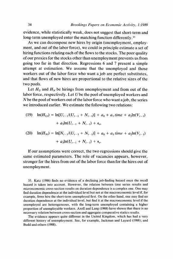
As we can decompose new hires by origin (unemployment, employ- ment, and out of the labor force), we could in principle estimate a set of hiring functions relating each of the flows to the stocks. The poor quality of our proxies for the stocks other than unemployment prevents us from going too far in that direction. Regressions 6 and 7 present a simple attempt at estimation. We assume that the unemployed and those workers out of the labor force who want a job are perfect substitutes, and that flows of new hires are proportional to the relative sizes of the two pools.
Let HU and HN be hirings from unemployment and from out of the labor force, respectively. Let U be the pool of unemployed workers and N be the pool of workers out of the labor force who want ajob, the series we introduced earlier. We estimate the following two relations:
(19) ln(Hut) = ln[Ut- ll(Ut- I + Nt- 1)] + ao + a, time + a2ln(Vt 1)
+ a3ln(Ut-I + Nt-1) + Et,
(20) ln(HNt) = ln[Nt-Il(Ut-I + Nt-1)] + ao + al time + a2ln(Vt 1)
+ a3ln(Ut- 1 + Nt_1) + Et.
If our assumptions were correct, the two regressions should give the same estimated parameters. The role of vacancies appears, however, stronger for the hires from out of the labor force than for the hires out of unemployment.
35. Katz (1986) finds no evidence of a declining job-finding hazard once the recall hazard is taken into account. However, the relation between time series results and microeconomic cross-section results on duration dependence is a complex one. One may find duration dependence at the individual level but not at the macroeconomic level if, for example, firms hire the short-term unemployed first. On the other hand, one may find no duration dependence at the individual level, but find it at the macroeconomic level if the unemployed are heterogeneous, with the long-term unemployed containing a higher proportion of unemployable workers. Axell and Lang (1988) have shown that there is no necessary relation between cross-section and aggregate comparative statics results.
The evidence appears quite different in the United Kingdom, which has had a very different history of unemployment. See, for example, Jackman and Layard (1988); and Budd and others (1988).

Olivier Jean Blanchard and Peter Diamond 35
Using the Estimated Function in the Minimalist Model
Having estimated the aggregate matching function, we now return to the minimalist model of the economy to examine its implications for the behavior of a model economy. After selecting all the parameters for the model, we calculate steady states for alternative levels of aggregate activity, c. If c follows a determinate sine wave, it generates counter- clockwise loops around the steady-state locus. The size of the loops indicates the difference that comes from integrating dynamics into the analysis instead of considering only steady states. Since the estimated matching function has a negative time trend, we then contrast cycles with parameters from early and late in the estimation period.
We take the matching function to be Cobb-Douglas, with constant returns and coefficient 0.4 on unemployment. We choose the scale parameter, A, which captures the constant plus the time trend in the estimated equation, to range from 1.30 at the beginning to 0.95 at the end. For q, the rate of quits (remembering that only quits that are replaced are relevant), we choose 0.01, which is the minimum manufac- turing quit rate in the period. The other parameters are then chosen to approximate sample averages for unemployment, vacancies, and mean hires. This leads to choices of 1.05 for (KIL), the ratio of potential jobs to workers; 0.023 for s, the reallocation parameter; and 0.925 for c, the potential activity level. These values imply, in turn, an arrival rate of good profitability shocks, ,rr, of 0.307 and an arrival rate of bad profit- ability shocks, rrO, of 0.025. For steady-state loci, we let c vary between 0.88 and 0.97. To trace out a cycle, we let c be a sine wave between 0.90 and 0.95, with a period of five years.
In figure 6, we show the time paths of new hires, H, unemployment, and vacancies when A was equal to 1. 1, representing the midpoint of our observation period. This figure can be compared with figure 5, which gives the observed time series. As with that figure, changes in vacancies show a small lead over changes in unemployment. In figure 7, we plot both the steady-state loci and the cycles of Uand Vfor the two parameters A = 0.95 and A = 1.3. The cycles are counterclockwise around the steady-state loci. As can be seen from the figure, the diagonal shift in the steady-state locus corresponds to an increase of roughly 1 percent in the unemployment rate. In contrast with this relatively small move, the small slope of the steady-state locus implies a much larger horizontal

36 Brookings Papers on Economic Activity, 1:1989
Figure 6. New Hires, Unemployment, and Vacancies Relative to the Labor Force, One Cycle, A = 1.1
Percent 10
8
6
4 Unemployment 4
-New hires Vacancies
2
o l l l l I L I 1 7 13 19 25 31 36 42 48 54 60
Time (months)
distance between the curves. The results show that the decrease in the productivity of the matching function is not very important if c ranges over the same values. However, if c is adjusted so that vacancies range over the same values, the decline in the matching function generates a large increase in unemployment. We return to these issues when dis- cussing the shift in the Beveridge relation later on.
This ends our discussion of the matching function. The other central element of our approach is our assumption that the economy is contin- uously subject to large flows of job creation and destruction. One may think-and we did-of using the evidence from gross flows of workers both at the aggregate level and in manufacturing to get at those flows. But these flows do not contain the evidence needed to get at those numbers. To take an example, our simple model implies that job terminations are equal to job separations minus quits because in the

Olivier Jean Blanchard and Peter Diamond 37
Figure 7. Beveridge Relation: Unemployment and Vacancies Relative to the Labor Force
Vacancy rate (percent) 5
4 _ A=0.95
A= 1.3
3
2
0 I I i I 2 4 6 8 10
Unemployment rate (percent)
model all quits are replaced. In actuality, quits are also used by firms to reduce their labor force, and not all quits are replaced. Thus, an estimate of job creations must embody assumptions as to the proportion of quits that is replaced. A more promising approach, to look at jobs directly, at employment changes by establishment, was followed recently by Davis and Haltiwanger, extending earlier work by Leonard.36 Their study, which constructs a quarterly time series for 1979 to 1983, suggests that job creations are indeed large and slightly procyclical, job destructions large and countercyclical. We have not explored the relation of their results to our approach further. In the last section, we use an indirect approach and use instead stock data to identify the importance and dynamic effects of cyclical, reallocation, and labor supply shocks.
36. Davis and Haltiwanger (1989); Leonard (1988).

38 Brookings Papers on Economic Activity, 1:1989
The Joint Behavior of the Labor Force, Unemployment, and Vacancies
We now return to the Beveridge relation. The relation between monthly unemployment and vacancy rates in the United States from 1952 through 1988, using the same measure of vacancies as earlier, is plotted in figure 8. The relation has two clear features. The first is the large thin loops around a downward-sloping locus. The other is the well- documented shift to the right over the postwar period.37 Interestingly, the shift has substantially reversed over the past four years: from the last month in 1984 through 1988, the vacancy rate has remained roughly constant, while the unemployment rate has decreased 2 percent.
Our earlier analysis suggests a simple interpretation of those move- ments: the large loops suggest that aggregate activity shocks dominate short- and medium-run movements in unemployment. The shifts to the right and more recently to the left suggest a role for changes in reallocation intensity or effectiveness, but over longer periods. This visual interpre- tation, however, can go only so far. It does not allow us to quantify the relative importance of the different shocks, nor does it clearly charac- terize the dynamic effects of the shocks on unemployment and vacancies. If there are more than two main sources of shocks, if, for example, shocks to the labor force are also important, the visual approach becomes potentially misleading. What this section does, therefore, is develop a simple but formal statistical interpretation of the data, which largely confirms and extends the initial visual impression.
The statistical approach is conceptually simple. A precise description is given in the appendix, but the logic underlying the various steps is easy to lay out.
From our theoretical analysis, we think of movements in the labor force, unemployment, and vacancies as coming from their dynamic responses to three types of shocks: shocks to aggregate activity, shocks to reallocation, and shocks to the labor force. Using the same notation as in the theoretical section, we denote the three variables by L, U, and V, respectively, and the three shocks by c, s, andf. These shocks are not observable and are likely to be serially correlated. We denote their
37. Abraham and Medoff (1982), for example.

Olivier Jean Blanchard and Peter Diamond 39
Figure 8. Beveridge Curve, 1952-88
Vacancy rate
(percent) 3.5
3.0.
2.5
88:1
2.0
1.5 75:2
82:12
1.0 4.0 6.0 8.0. 10.0 12.0
Unemployment rate (percent)
innovations-the white noise residuals that one would obtain from a regression of those shocks on their lagged values, were those shocks observable-by Ec, E,, and Ef. Thus, putting the two sources of dynamics together, we can think of the movements in L, U, and V as coming from the dynamic effects of the three innovations, Ec, E,, and Ef.
We then estimate the dynamic process characterizing the joint move- ments of L, U, and V, using monthly data from 1952 through 1988, by means of a vector autoregression. We use the labor force and unemploy- ment series from the household survey, and use for vacancies the adjusted help-wanted series described in the previous section. The vector autoregression gives L, U, and V as functions of their lagged values and of three reduced-form, white noise innovations-the monthly move- ments in L, U, and V that cannot be predicted from lagged values. Denote the three reduced-form innovations by 1, u, and v, respectively. Under our interpretation, these reduced-form innovations are linear

40 Brookings Papers on Economic Activity, 1:1989
combinations of the 's. That is, the unexplained movement in unem- ployment during a month comes from innovations in aggregate activity, from innovations in the intensity of reallocation, or from innovations in the labor force. If we knew those linear combinations, we could go from 1, u, and v back to the E's and characterize the dynamic effects of each of the E's on L, U, and V. The data do not, however, tell us anything about those linear combinations. Thus, to recover them, we must make identification assumptions. We make the following assumptions.
First, we assume that the three innovations Ef, Es, and E are uncorre- lated. One can think of many reasons why this may not be exactly the case, but we believe it to be an acceptable approximation. The assump- tion of zero correlation between aggregate activity and reallocation innovations requires some discussion. Consider, for example, changes in the price of oil. An oil price increase may well lead to a positive realization of Es (more required reallocation) and a negative value of Ec (an aggregate demand contraction through income effects); but, sym- metrically, an oil price decrease also corresponds to a positive realization of Es (more required reallocation) and a positive realization of Ec (an aggregate demand expansion through the same income effects). Thus, oil price shocks lead to a zero correlation between c and s. A similar argument also holds if, for example, changes in aggregate activity lead to larger required reallocation. But one can also think of counterexam- ples. Increases in reallocation may be systematically associated with scrapping of old equipment and surges of investment, leading to a positive correlation between E and Ec.
Second, we assume that Ec affects unemployment and vacancies in opposite directions for at least n months and that E affects them in the same direction for at least n months. We choose n to be 9; results are not very sensitive to the exact choice of n, say between 5 and 10 months. These assumptions in effect define E and E, and it is important to note that these are more general definitions than those used in our theoretical model. For example, the definition of Es is consistent with positive reallocation shocks first leading to job destruction and an increase in unemployment, and leading only over time to the creation of new jobs and the posting of vacancies. The definition of Ec is consistent with negative changes in aggregate activity leading first to a decrease in vacancies, then to layoffs, and so on.
Third, we assume that innovations in the labor force respond only to
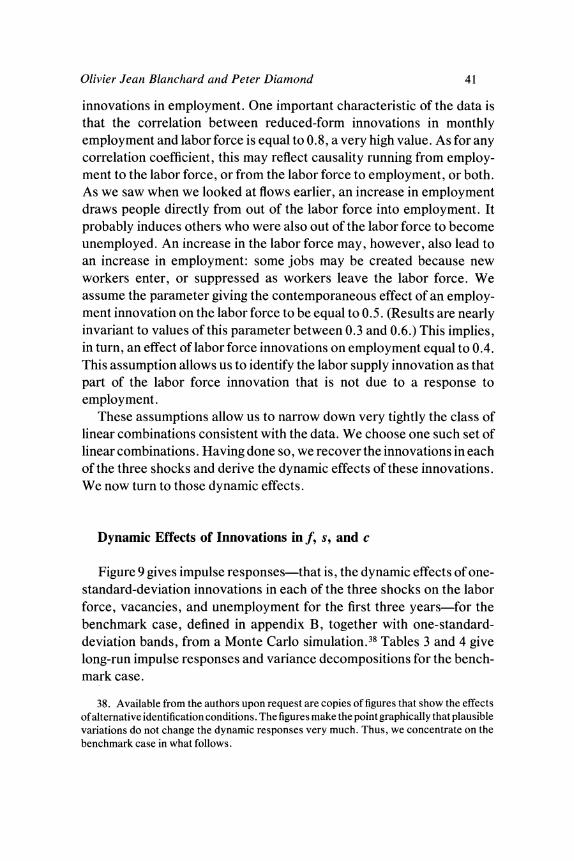
Olivier Jean Blanchard and Peter Diamond 41
innovations in employment. One important characteristic of the data is that the correlation between reduced-form innovations in monthly employment and labor force is equal to 0.8, a very high value. As for any correlation coefficient, this may reflect causality running from employ- ment to the labor force, or from the labor force to employment, or both. As we saw when we looked at flows earlier, an increase in employment draws people directly from out of the labor force into employment. It probably induces others who were also out of the labor force to become unemployed. An increase in the labor force may, however, also lead to an increase in employment: some jobs may be created because new workers enter, or suppressed as workers leave the labor force. We assume the parameter giving the contemporaneous effect of an employ- ment innovation on the labor force to be equal to 0.5. (Results are nearly invariant to values of this parameter between 0.3 and 0.6.) This implies, in turn, an effect of labor force innovations on employment equal to 0.4. This assumption allows us to identify the labor supply innovation as that part of the labor force innovation that is not due to a response to employment.
These assumptions allow us to narrow down very tightly the class of linear combinations consistent with the data. We choose one such set of linear combinations. Having done so, we recover the innovations in each of the three shocks and derive the dynamic effects of these innovations. We now turn to those dynamic effects.
Dynamic Effects of Innovations in f, s, and c
Figure 9 gives impulse responses-that is, the dynamic effects of one- standard-deviation innovations in each of the three shocks on the labor force, vacancies, and unemployment for the first three years-for the benchmark case, defined in appendix B, together with one-standard- deviation bands, from a Monte Carlo simulation.38 Tables 3 and 4 give long-run impulse responses and variance decompositions for the bench- mark case.
38. Available from the authors upon request are copies of figures that show the effects of alternative identification conditions. The figures make the point graphically that plausible variations do not change the dynamic responses very much. Thus, we concentrate on the benchmark case in what follows.

I I~~~~~~~~~~~~~~~~~~~~~~~~~~~~~~~~~~~~~~~~~~~~~~~~~~~~~~~~~~~~~~~~~~~~~' I U~~~~~~~~~~~~~~~~~~~~~~~~~~~~~~~~~~~~~~~~'
I I I ~~~~~~~~~~~~~~~~~~~~~~~~~ E~~~~~t I I~~~~~~~~~~~~~~~~~~~~~~~~~~~~~~~~~~~~~~~~~~~~~~~~~~~~~~~~~~~~~~~~~~~~~'
I I~~~~~~~~~~~~~~~~~~~~~~~~~~~~~~4
m 20~~I
U) ~ ~ ~ " C's
\I~~~~~~~~~~~~~~~~~~~~~~~~~~~~~~~~~~~~~~~~~~~~~~I
/ I,~~~~~~~~~~~~~~~~~~~~~~~~~~~~~~~~~~~~~~~~~~~~~~~~~~~~~~~~~~~~~~~~~~~~~I N~~~~~~~~~~~~~~~~~~~~~~~~~~~I
I I I - E~~~~~~~~~~~~~~~~~~~~~~~~~~~~~~~~~~~~~- I i I C~~~~~~~~~~~~~~~~~~~~~~~~~~~~~~~~~~~~~~~~~~~~~~~~~~~~~~~~~~~~~~~~~~~~~~~~~~~~~~~~~~~~~I1
/ ~~~~~~~~~~~~~~~~~~~~~~~~~~~~~~O~~~~~~' '
40- C's / /

Olivier Jean Blanchard and Peter Diamond 43
Table 3. Impulse Responsesa
L V U Shock Months (x 1-2) (X 10-3) (X 10-2)
Long-run impulse responsesb Ef 1 0.30 -0.05 0.11
100 0.30 0.08 0.05 200 0.34 0.10 0.03
E, 1 0.04 0.53 - 0.07 100 0.04 0.02 - 0.02 200 -0.01 0.00 0.00
E 1 -0.01 0.05 0.13 100 0.23 0.05 0.07 200 0.36 0.09 0.05
a. Identification assuming 0 = 0.4, ot = 2.2; 0 and ot are defined in Appendix B. b. Impulse responses for the first 36 months are plotted in figure 9.
Table 4. Variance Decompositionsa
Variable Months Ef E, es
Proportion of variance due to shock L 1 0.89 0.02 0.08
36 0.75 0.17 0.07 100 0.68 0.08 0.22 200 0.58 0.02 0.39
V 1 0.01 0.97 0.01 36 0.06 0.86 0.07
100 0.07 0.85 0.07 200 0.10 0.80 0.09
U 1 0.33 0.13 0.53 36 0.04 0.86 0.09
100 0.11 0.61 0.26 200 0.14 0.49 0.36
a. Identification assuming 0 = 0.4, ot = 2.2.
Overall, the qualitative dynamic effects are consistent with the predictions of the formal model. This has to remain a vague statement, given that all we observe is a convolution of the lag structure implied by the model and the lag structure of the shocks. Without some restrictions on the joint process of the shocks, such as the assumption that the three shocks are uncorrelated at all leads and lags, any set of estimated impulse responses is a priori consistent with the model. In our interpretation of the results below, we make indeed this implicit restriction. From figure

44 Brookings Papers on Economic Activity, 1:1989
9, which spans the first three years after a shock, we see the main features of the results as being the following.
The effects of labor supply innovations, Ef, on the labor force quickly decrease to about two-thirds of the initial impact, and then stabilize at that level. This is suggestive of two components: one, new entrants who come in and stay and, the other, workers with marginal attachment who go in and out of the labor force. The effect on unemployment dies out within a year: the increase in the labor force has by then translated into an increase in employment. The short-run dynamic response thus appears consistent with the predictions of equation 16, the model in which capital is fixed; the longer-run response appears consistent with the predictions of the model composed of equations 6' and 7', in which the number ofjobs moves with changes in the labor force.
Positive aggregate activity innovations, E,, lead to a sustained increase in vacancies and a sustained decrease in unemployment, as well as an increase in the labor force. The effects on unemployment and vacancies are hump-shaped, peaking within less than a year, and all but disappear- ing after three years. Vacancies peak one or two months before unem- ployment bottoms out. While aggregate activity shocks have negligible long-run effects on unemployment or vacancies, they have a long-run effect on the labor force, an effect not predicted by our analysis and suggestive of hysteretic effects of changes in activity on participation.
Positive reallocation innovations, Es, lead-by construction-to in- creases in both unemployment and vacancies. But their dynamic effects differ from those predicted by our theoretical analysis in two ways. First, the increase in unemployment precedes the increase in vacancies. The increase in unemployment is highestjust after the shock, while vacancies increase to peak after roughly a year. This suggests a process in which higher reallocation intensity leads first to the loss ofjobs, followed only over time by the creation of new jobs, a plausible dynamic process but one we did not build in our model. Second, while the initial effects of an increase in reallocation intensity are to increase unemployment and decrease the labor force, the effect on the labor force becomes positive in the medium and long run; a tentative explanation is again that of hysteretic effects of shocks on participation. Most of those who lose their jobs remain in the labor force, while new jobs, which may appear in new locations, draw in new workers.
The picture given by figure 9 is one in which aggregate activity shocks

Olivier Jean Blanchard and Peter Diamond 45
largely dominate fluctuations in unemployment and vacancies. This picture is sharpened in tables 3 and 4. While long-run impulse responses are imprecisely estimated, the results in table 3 are, taken at face value, interesting. The effects of aggregate activity innovations, while large in the short and medium run, disappear nearly completely in the long run. In contrast, both reallocation and labor force shocks appear to have long-run effects on unemployment and vacancies. This suggests that nonstationarity in the three series is due to the long-run effects of labor force and reallocation shocks rather than to the long-run effects of aggregate activity shocks.39
Even if aggregate activity shocks have no long-run effect, variance decompositions in table 4 show, however, that, given their contribution to short- and medium-run movements, aggregate activity shocks account for a very large proportion of movements in both unemployment and vacancies at all horizons. The proportion is smaller for unemployment at short horizons, where labor force and reallocation shocks are impor- tant. The proportion also declines slowly with the horizon, reflecting the small long-run effect of aggregate activity shocks described earlier, but remains large even after 18 years.
Back to the Beveridge Curve
We can now return to the familiar Beveridge curve representation and decompose the movements in the unemployment and the vacancy rates into the movements due to labor supply, reallocation, and aggregate activity shocks. We do this in figures 10 and 11. Figure 10 gives the loci traced by the unemployment rate, UR, and the vacancy rate, VR, for the first 60 months following a one-standard-deviation innovation in each of the shocks.40 Figure 11 decomposes the historical movements in the Beveridge curve into the components due to each of the three shocks and a deterministic component, the movement in UR and VR that would have occurred, had all realizations of shocks been identically equal to
39. If aggregate activity innovations truly had no effect on the variables in the long run, this would imply the existence of one cointegrating vector across the three variables. As we see in Appendix B, however, there is no evidence that such a vector exists in the data.
40. Figure 10 contains exactly the same information as figure 9. It is just another way of looking at the dynamics of unemployment, vacancies, and the labor force.
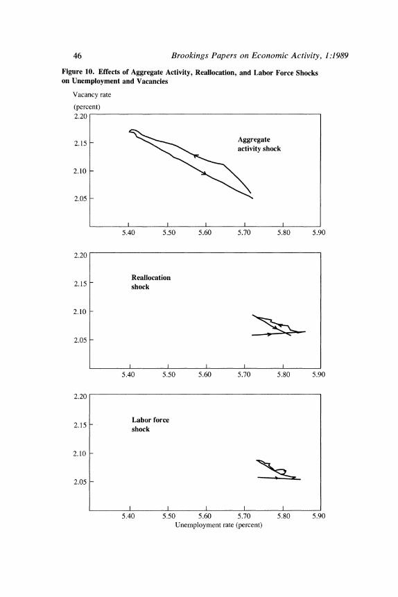
46 Brookings Papers on Economic Activity, 1:1989
Figure 10. Effects of Aggregate Activity, Reallocation, and Labor Force Shocks on Unemployment and Vacancies
Vacancy rate
(percent) 2.20
2.15 -Aggregate activity shock
2.10 -
2.05 -
I I I I 5.40 5.50 5.60 5.70 5.80 5.90
2.20
Reallocation 2.15
- shock
2.10 -
2.05
l I I
5.40 5.50 5.60 5.70 5.80 5.90
2.20
Labor force 2.15 -shock
2.10-
2.05 -
5.40 5.50 5.60 5.70 5.80 5.90 Unemployment rate (percent)

Olivier Jean Blanchard and Peter Diamond 47
zero during the period. (While we do not allow for a time trend when doing estimation, the system will exhibit time trends if some of the estimated roots are very close to unity, and the constant terms of the regressions are different from zero.) From these figures, we draw two sets of conclusions.
In the short and medium run, aggregate activity shocks have, by far, the largest effects on the unemployment and vacancy rates, and generate the predicted counterclockwise loops. Reallocation and labor supply shocks have small effects, and the movements implied by reallocation shocks are initially flatter than the movements along a 45 degree line predicted by the theory. Our findings confirm our initial visual impression and the conclusions of Abraham and Katz in the debate triggered by Lilien on the importance of sectoral shocks to aggregate fluctuation.41 Our approach to the interpretation of the joint movement of vacancies and unemployment is more formal than theirs but, on that point, ends with the same conclusion. There are large flows of job creation and destruction in the United States, but changes in the intensity of the reallocation process do not appear to be an important determinant of unemployment fluctuations. In the long run, however, effects of aggre- gate activity shocks disappear, while effects of reallocation and labor supply shocks do not. This leads to the second set of conclusions.
Part of the shift in the Beveridge relation in the postwar period is attributable to the long-run effects of reallocation shocks, as is made clear by figure 11. The movements due to changes in aggregate activity given in the figure are large but account for none of the drift in the relation over the period. The movements due to labor supply shocks account for small movements of UR and VR and, again, for none of the drift. The movements due to reallocation activity, however, account for a steady movement of the unemployment rate upward, by 2 percent from the late 1960s to 1984, followed by a decrease of roughly 1 percent since. Long-run effects of reallocation shocks, however, are not the whole story. The deterministic component (trend) shown in the figure traces an increase in unemployment of 3 percent from the early 1950s to 1975, followed, again, by a decrease of 1 percent since, without much change in the vacancy rate over the whole period. Where does the deterministic component in turn come from? It may come from trends in the underlying shocks, such as, for example, movements in reallocation intensity steady
41. Abraham and Katz (1986); Lilien (1982).

48 Brookings Papers on Economic Activity, 1:1989
Figure 11. Decomposition of Beveridge Relation into Components Due to Trend, Reallocation Shocks, Labor Force Shocks, and Aggregate Activity, 1952-88
Vacancy rate
(percent) 3.5
March 1969
Aggregate 3.0 - activity
shock
2.5-
2.0-
15 November
1.0 I l 4.5 6.0 7.5 9.0
Unemployment rate (percent)
Vacancy rate (percent) 3.5
Labor 3.0 - force
shock
2.5
2.0 -
1.5-
1.0 l 4.5 6.0 7.5 9.0
Unemployment rate (percent)

Olivier Jean Blanchard and Peter Diamond 49
Vacancy rate
(percent) 3.5
Reallocation 3.0 - shock
2.5
September 1960
2.0 October 1983
1.5
1.0 I , 4.5 6.0 7.5 9.0
Unemployment rate (percent) Vacancy rate (percent) 3.5
Trend 3.0-
2.5 _
December 1988
January 1952 v \ 2.0 August 1975
1.5 -
1.0 4.5 6.0 7.5 9.0
Unemployment rate (percent)
50 Brookings Papers on Economic Activity, 1:1989
enough to be captured by a deterministic rather than by the stochastic component, or from trend changes in matching, such as, for example, an increased geographical dispersion of workers and new jobs. The evidence presented earlier suggests that trend changes in matching, which we find in our estimation of the matching function for the period 1968 to 1981, account for a good part of this deterministic trend.42
Conclusions
We have modeled a U.S. labor market with large numbers of jobs being constantly created and destroyed. Such a model, rather than a representative agent model, or a centralized bargaining model with immobile labor, is, we think, the appropriate starting point for macro- economics.
We have focused on the matching process and the sources of shocks in the economy. Although jobs and workers are efficiently matched, unemployment and vacancies coexist because of the sheer volume of jobs being created and destroyed. Flows of newly hired workers, we find, depend on both unemployment and vacancies. As the comovement of unemployment and vacancies over the postwar period shows, short- and medium-term fluctuations in unemployment have been due mainly to aggregate activity shocks, shocks that lead to both more (less) job creation and less (more) job destruction, rather than to changes in the degree in reallocation intensity, which lead to parallel movements in job creation and job destruction.
We have, however, stopped well short of discussing issues of "equi- librium unemployment. " The reason is that, as a formalization strategy, we have taken the potential level of activity, c, as well as the level of K, as given. Both, in turn, depend on wages, thus on wage determination.
42. We intend to follow up on this statement and come up with a more specific estimate. We have run into the following difficulty. The theoretical model suggests that decreases in matching effectiveness should lead, like reallocation shocks, to movements along a 45 degree line. This suggests that what is needed to generate the observed flat shift is a combination of elements, such as an increase in s and a decrease in c. The estimated effects of reallocation shocks are also flat, however, which suggests that our theoretical model may not be the right framework to use for this computation.

Olivier Jean Blanchard and Peter Diamond 51
Thus, the next step in building a model of equilibrium unemployment is to draw out the implications of this approach for wage determination.
Our model has an implicit theory of wage determination. Wages are set to allow a match to happen if it is mutually profitable. A natural and appealing formalization of wage setting that has this property is that the surplus from the match between a worker and a firm is shared in some proportion, an assumption of Nash bargaining. This assumption implies that wages depend on the ratio of vacancies to unemployment, which reflects the relative bargaining strengths of workers and firms. The higher are vacancies given unemployment, the higher the wage; the higher is unemployment given vacancies, the lower the wage. Thus, it matters for wages whether unemployment is due to increases in reallocation intensity or instead to a negative aggregate activity shock. The model suggests both an integrated way of thinking about the Phillips curve and the Beveridge curve and a way to learn about the workings of the labor market and the source of the shocks from a joint examination of unemployment, vacancies, and wages, an avenue explored by Robert Solow in his 1964 Wicksell lectures, or, more recently, by Richard Layard and Steve Nickell in their analysis of unemployment in the United Kingdom.43
This theory of wage determination may not, however, capture impor- tant aspects of the labor market. A more ambitious task will be to consider wage-setting mechanisms that sometimes prevent mutually beneficial matching from taking place. We have in mind here preset wages or union-negotiated wages. Indeed, one of the challenges of this approach is to combine centralized wage setting-which, along with wage drift, is also characteristic of the U.S. labor market-and a description of the market that allows for the large flows of workers we have documented. These extensions are on our agenda.
43. Solow (1964); Layard and Nickell (1986).

52 Brookings Papers on Economic Activity, 1:1989
APPENDIX A
Data Sources and Construction
New Hires
New hires are constructed as gross flow from unemployment to employ- ment, plus gross flow from out of the labor force to employment, plus estimated employment-to-employment quits, minus estimated recalls.
Gross flow from unemployment to employment and gross flow from out of the labor force to employment: in each case, the sum of male and female gross flows, as adjusted by Abowd and Zellner (in data from the authors), deseasonalized by removing all power from frequencies in a band around seasonal frequencies.
Estimated employment-to-employment quits: 0.4 times quit rate in manufacturing times aggregate employment from household survey. Quit rate in manufacturing (RQ UITM) and aggregate employment (EHH) from Data Resources, Inc., U.S. Central Data Bank.
Estimated recalls: 1.5 times (manufacturing accession rate minus manufacturing new hire rate) times manufacturing employment from establishment survey. New hire rate (NHR) from DRI. Manufacturing accession rate (LPACCM) and manufacturing employment (LPEM) from Citibase, Citicorp Databank Services.
Pool of Workers
Unemployment: total unemployment from the household survey (UHH) from DRI.
Persons not in the labor force wanting a job now: quarterly series, Employment and Earnings, table A-53.
Job losers on layoff: Employment and Earnings, table A-14. Long-term unemployment: persons unemployed for 27 weeks or more
(U27&W) from DRI. Short-term unemployment: persons unemployed for less than 27
weeks (UHH - U27& W) from DRI.

Olivier Jean Blanchard and Peter Diamond 53
Vacancies
Vacancies: help-wanted index (LHELX) from Citibase times adjust- ment factor. The adjustment factor is obtained by first regressing the logarithm of the adjustment factor in Abraham (1987), table A. 1, on a quadratic in time forthe period 1960 to 1985. During thatperiod, Abraham estimates that the ratio of the help-wanted index to vacancies increased 35 percent. The estimated exponential trend is then assumed to hold for the period 1952 to 1988 and used to multiply the help-wanted index series for that period. The level of the resulting series is adjusted so that the average vacancy rate is equal to 2.2 percent for the period 1969 to 1981.
Labor Force
Labor force: Civilian labor force from household survey (LC) from DRI.
APPENDIX B
Construction and Identification of the VAR Representation
THIS APPENDIX shows how we recover the shocks, their dynamic effects, and their contribution to movements in unemployment, vacancies, and the labor force.
From the Theoretical Model to the VAR Representation
Let X = [L, V, U]' be the vector composed of the labor force, vacancies, and unemployment (where L, V, and U denote either levels or logarithms, an issue taken up later). Let Z = [f, c, s]' be the vector of labor supply, aggregate activity, and reallocation shocks respectively.

54 Brookings Papers on Economic Activity, 1:1989
We can think of our theoretical model as yielding a dynamic relation between X and Z of the form
(B. 1) X = B(L)Z, B(O) = Bo,
where B(L) is an infinite-order matrix lag polynomial. In writing equation B. 1 as we do, we take two shortcuts. The first is
that the theoretical analysis is presented in continuous time while equation B.1 is, for estimation purposes, written as a discrete time system. Estimation of a continuous time model with discrete time data raises a number of well-known issues, which we shall not discuss further. The second and more important shortcut is that the theoretical model is nonlinear, both in the variables and in the shocks, while equation B. 1 is linear in both. There is no simple way of handling those nonlinearities without estimating a tightly specified structural model, something we do not want to do at this point. We therefore estimate a linear system, which must be thought of as a linear approxirnation to the true joint process. An indirect test of whether this approximation is acceptable is provided by subsample stability tests given below, as the subsamples have different mean unemployment and vacancy rates.
Equation B .1 gives the behavior of X as a function of Z, the vector of shocks. Let Z itself follow a linear stochastic process given by
(B.2) Z = C(L)E, where E(EE') = V, CO = I,
where E [Ef, E,, EJ' is the vector of white noise innovations tof, c, and s, and CO I is a normalization. Then, replacing equation B .2 in equation B. 1 gives X as a distributed lag of e:
(B. 3) X = A(L)E, where A(L) = B(L)C(L), E(EE') = V.
From the normalizations above, AO = Bo. The matrix polynomial A(L), which gives the effects of innovations in the underlying shocksf, s, and c, is a convolution of the matrix polynomials in equations B.2 and B.3. Put another way, the dynamic behavior of X comes both from the intrinsic dynamics of the system, characterized by B(L), and from the dynamics of the shocks themselves, characterized by C(L).
With clear abuse of language, we refer to equation B .3 as the structural model in what follows. We do so to distinguish it from the vector

Olivier Jean Blanchard and Peter Diamond 55
autoregression (VAR) reduced form. Estimation of a VAR does not yield equation B.3 directly but rather the reduced form:
(B.4) X = D(L),q, E(rlq') = 1, Do = I,
where q = [1, v, u]' is the vector of reduced-form innovations, the vector of unexpected movements in L, V, and U, and the VAR is written in moving average form. From equations B.3 and B.4, it follows that - = BoE and that A(L) = D(L)BO, so that knowledge of Bo is sufficient to go from equation B.4 to equation B.3.
Our empirical strategy is therefore the following. We first estimate the reduced-form equation B.4. We then make identification restrictions, which allow us to identify Bo and to go back from the reduced form to the structural model equation B.3. We can then characterize not the dynamic effects of the shocks themselves, but the dynamic effects of innovations to those shocks on the labor force, vacancies, and unem- ployment.
Reduced-Form Estimation
We use monthly data, from 1952 through 1988 (444 observations). We use the labor force and unemployment series from the household survey, and, for vacancies, the adjusted help-wanted series described in Appen- dix A.
The theoretical model is neither linear nor loglinear. To allow for geometric growth, we perform estimation using logarithms of the varia- bles. We have also looked at estimation results using logarithms of the labor force, employment (rather than unemployment), and vacancies, which imply a more approximately linear relation between unemploy- ment and the labor force; results are very similar. All variables are normalized (that is, the logarithms are multiplied by an appropriate constant) so that all the coefficients reported below have the interpreta- tion of derivatives, evaluated at sample means.
We use levels (of logarithms) rather than first differences or cointe- grated estimation. The evidence strongly suggests that all three variables are nonstationary, whether or not a deterministic time trend is included. Results of cointegration tests among the three variables, or between

56 Brookings Papers on Economic Activity, 1:1989
Table B-1. Results of Cointegration Tests for Unemployment, Vacancies, and the Labor Force, 1952-88
t-statiStiCa
Test DF ADFI ADF2
Among L, U, V - 2.33 -1.10 -2.49 Critical valueb (-3.47) (-3.51) (-3.83)
Between L, V - 1.38 -2.44 -2.31 L, U -0.78 -1.71 -2.99 U, V - 1.85 - 2.59 -0.92
Critical valueb (-3.02) (-2.98) (-3.51)
a. DF: t-statistic on coefficient on x_ X in a regression of ax on x1. ADFI: t-statistic on coefficient on x_ in a regression of Ax on x - and twelve lags of Ax. ADF2: same as ADFI, but with time trend included in first stage regressions. In each case x is the residual in a regression of the first variable of the cointegration test on the remaining one or two variables.
b. Critical values at the 10 percent level (from Engle-Yoo, 1987).
pairs of variables, with or without a deterministic trend, are given in table B-1. There is no evidence of cointegration among the three series, or between any pair of series. We prefer, nevertheless, not to impose nonstationarity of unemployment rates or vacancy rates, and thus do estimation in levels. The usual caveat about standard deviations and other statistics reported below applies.
On the basis of likelihood ratio tests, we estimate the VAR, equation B .4, allowing for 12 lags on each variable. We have examined subsample stability, cutting the sample at the end of 1972. The hypothesis of subsample stability of the VAR is rejected by a maximum likelihood test at approximately the 2 percent level; but we find little difference across subsamples between the implied impulse responses (the definition of those impulse responses is given below). Thus, we treat the sample as a whole in what follows.
The results of estimation are summarized in table B-2, which also gives F-tests associated with the hypotheses that the set of coefficients on each variable in each equation is equal to zero.
An economic analysis of the properties of the estimated dynamic system must await identification. Note, however, the very high signifi- cance level of vacancies in the unemployment equation; this is due in part to the effect of vacancies lagged once, which affect unemployment with a coefficient of close to minus one. Given the normalization we use, the implication is that, other things being equal, one more vacancy this month is associated with one fewer worker unemployed next month.

Olivier Jean Blanchard and Peter Diamond 57
Table B-2. Coefficients of Independent Variables: Sum and Significance Level of the Set, 1952-88 a
Left-hand side variable
L U V
Significance level of the set of coefficients onb L 0.00 0.05 0.81 U 0.04 x 10- 0.00 0.24 V 0.05 0.16 x 10⁻¹o 0.00
Sum of coefficients on L 0.98c 0.00 0.00
U 0.06c 0.99c 0.00 V 0.26c -0.02 0.96c
a. All regressions in levels of natural logs, with 12 lags for each variable and a constant. b. Numbers reported are F-test results associated with the hypothesis that the set of coefficients on a given right-
hand variable is equal to zero. c. Significantly different from zero at I percent level.
Identification
What we get from VAR estimation is the set of reduced-form residuals. Denote by 1, v, and u the reduced-form innovations in L, V, and U (the residuals from estimation of the reduced form). Table B-3 gives the standard deviations as well as the correlations between those innova- tions. Because we find it more intuitive to think in terms of the labor force, vacancies, and employment, the table also gives standard devia- tions and correlations between 1, v, and e, where e is defined as 1- u, and thus has the interpretation of the innovation in employment. The striking characteristic of this table is the large correlation between employment and labor force innovations.
Table B-3. Correlations between Reduced-Form Innovations, 1952-88
Correlations Standard Innovation 1 u v deviation
I 1.00 0.27 0.01 ir/=0.00320 u 1.00 -0.34 = 0.00190 v 1.00 = 0.00054
I e v I 1.00 0.82 0.01 u1=0.00320
ea 1.00 0.22 0e=.00290 v 1.00 = 0.00054
a. e = 1- u.

58 Brookings Papers on Economic Activity, 1:1989
Under our interpretation of the joint behavior of L, V, and U, those correlations reflect thejoint dependence of the reduced-form innovations on Ef, Ec, and Es, the labor supply, aggregate activity, and reallocation innovations, respectively. We specify the following set of relations between structural and reduced-form innovations as
1 = 0(-Es + a%Ec) + Ef,
(B. 5) v = IEs + EC,
e = -es + ?-Ec + XEf.
We expect all parameters as defined to have a positive sign. Positive reallocation innovations are assumed to increase vacancies, decrease employment, and, through employment, decrease the labor force. Pos- itive aggregate activity innovations increase vacancies and employment, and, through employment, increase the labor force. Labor supply innovations increase the labor force and may increase employment. All these effects-except for the effects of labor supply innovations on employment, to which we return below-are what is predicted by our minimalist model, extended to allow for endogeneity of the labor force, the model given by equation 16. If the time unit were short enough, the coefficients in equation B .5 would correspond to the instantaneous direct effects of each of the shocks on each of the three variables L, V, and U in that model. As the time unit increases, indirect effects through movements in L, V, and U become relevant; we shall ignore these indirect effects in thinking about identification. The innovations are normalized by assuming that the effect of the labor supply innovation on the labor force is one, the effect of the aggregate activity innovation on vacancies is one, and the effect of the reallocation innovation on employment is minus one.
We then achieve identification by a set of three assumptions. First, we assume that the three structural innovations Ef, Es, and Ec are
uncorrelated, that the matrix Vin equation B.2 is diagonal. This assump- tion is discussed in the text.
Our formal model implies that an exogenous increase in the labor force should have no instantaneous effect on employment, thus that X in the third part of equation B.5 is equal to zero. In this case, labor supply innovations, Ef, can be obtained as the residuals of a regression of 1 on e, the first part of equation B.5. This leads to an estimated coefficient of 0

Olivier Jean Blanchard and Peter Diamond 59
of 0.8, a within-the-month increase in the labor force of 8 workers for any 10 workers employed; this estimated coefficient reflects the very high correlation between employment and labor force innovations in the correlation matrix of the reduced-form residuals, which was reported in table B-3.44 We find the estimated value of 0 implausibly high, and we are led to conclude that an exogenous increase in the labor force is probably associated with some increase in employment, that some jobs are created because new workers enter, or suppressed as existing workers leave, the labor force. Thus, we allow for a positive value of X. A given value of X implies a given value of 0 and vice versa. In what follows, we choose a value of 0 equal to 0.4, which implies a value of X of 0.5. We have found that impulse responses are nearly invariant to values of 0 between 0.3 to 0.6, which imply values for X of 0.57 and 0.34, respectively.4
Finally, we identify aggregate activity and reallocation innovations, EC and E, by assuming that E, affects unemployment and vacancies in opposite directions for at least n months and that E, affects them in the same direction for at least n months. This in effect defines EC and E and, as discussed in the text, these are more general definitions than those used in our theoretical model. This set of assumptions imposes a set of tight restrictions on the pair (ac, 1). Given one of the two parameters, the other is identified.46 For each value of a-, we can obtain 1, and derive the
44. We have explored the robustness of this high correlation at length. To see whether it came in part from common measurement errors in employment and the labor force, we constructed the labor force series by adding to unemployment the employment series from the establishment survey rather than from the household survey. The correlation between I so constructed and e defined again as 1- u is lower, but still equal to 0.7.
We would expect seasonal flows into the labor force to be associated with job creation. Thus, to see whether the results could be due to seasonal effects left in the series after X1I deseasonalization, we deseasonalized the non-seasonally-adjusted series by using fre- quency domain deseasonalization with large seasonal bands. The correlation so obtained is still equal to 0.74.
45. The model so defined is actually overidentified. One can relax this overidentification by allowing for an effect of Ef on v as well. This coefficient, when estimated, is nearly equal to zero.
46. The problem is very similar to the standard problem of identification of the supply and the demand curve. Given an assumed slope for the demand curve, we can identify the supply curve, and reciprocally. Here, we have two shocks, E, and E,. The first one affects both variables in the same direction, the second affects them in opposite directions. Knowing the effects of the first one allows one to recover the effects of the second.

60 Brookings Papers on Economic Activity, 1:1989
impulse responses of all variables with respect to each of the shocks. We then look for values of ac such that the effects of EC be of opposite signs on unemployment and vacancies, and the effects of E, be of the same sign on unemployment and vacancies, for at least n months.47 For n equal to nine months, this leads to a narrow band of values for a-, from 1.8 (for which e = 0.00) to 3.0 (for which e = 0.06). For values outside the band, impulse responses have unemployment and vacancies moving generally together, so that both shocks look like aggregate activity shocks. One can therefore see our identification restrictions as making the strongest case for reallocation shocks. We choose a value of ax equal to 2.2 (which implies e = 0.02); we also have calculated impulse responses for values of ac of 2.0 and 2.8 and found them to be very similar to those obtained under ac = 2.2. Note, for future reference, that the values of 1 in the acceptable range are far smaller than the value of 1, implied by our simple model (for the specific definition of s used there).
The benchmark case discussed in the text uses values of 0.4 for 0 and 2.2 for ac. Impulse responses obtained under the alternative assump- tions-0 = 0.3, ac = 2.2; 0 = 0.6, ac = 2.2; 0 = 0.4, a = 2.0; and 0 =
0.4, ac = 2.8-are available upon request. Given those assumptions, we can estimate, using the method of
moments, the parameters and standard deviations of the E's in equation B.5. Having recovered Bo, we can recover the structural model and characterize the dynamic effects of the 's on L, V, and U.
47. To pursue the analogy of the previous footnote, this is the dynamic equivalent to the question: what assumed slopes for the supply curve are consistent with the demand curve sloping downwards ?

Comments and Discussion
Robert E. Hall: The paper by Olivier Blanchard and Peter Diamond is a careful exercise in model building. It does not try to settle controversial questions in macroeconomics. Though its goals are more modest than those of many Brookings papers, the paper is highly instructive on some major issues about the operation of the labor market. The authors see job-worker matching as another substantive economic activity, capable of description by a production function. I think the resulting intellectual discipline is a big step forward.
One problem facing this type of research is the disproportionate role of certain types of workers in the turnover process. On the one hand, the labor market has high average turnover; about 4 percent of workers take new jobs each month. On the other hand, about 50 percent of workers at any one time have been on the job for three years or more; their turnover rates are only a fraction of a percent a month. Teenagers and other high-turnover workers with very brief previous employment dominate the turnover process. It is crucial to understand that the matching function estimated in this paper tells us how teenagers find jobs in services and trade, not how the market works for experienced workers with substantial human capital. With considerable additional effort, Blanchard and Diamond might be able to estimate a disaggregated model, using microeconomic data for workers and detailed help-wanted advertising data for vacancies.
Blanchard and Diamond do not hide the infirmities of the data. Gross flows data from the Current Population Survey are well known to have substantial biases; the results in the paper are very dependent on the accuracy of the Abowd-Zellner adjustments. Katharine Abraham's work has shown the strengths and weaknesses of help-wanted advertising as
61

62 Brookings Papers on Economic Activity, 1:1989
a measure of the vacancy rate. A particular problem with the help- wanted data is the lack of information about the trend in the relation of advertising to vacancies, which is an important issue in Blanchard and Diamond's paper. Finally, unemployment is notoriously hard to mea- sure. Only about half the people who are not working but say they want to work are counted as unemployed. Only about half those counted as unemployed consider job search their primary activity in the survey week of the CPS. Again, there may be important changes over time in the relation between measured unemployment and the volume of job- seeking activity.
One of the most important contributions of the paper is the develop- ment of a matching function for the U. S. economy. Stocks of unemployed workers and vacant jobs are the inputs, and job matches (new hires) are the output. Estimates of the matching function by ordinary least squares are likely to understate the elasticities with respect to both U and V. A random shift in matching affects both U and V: each spontaneous new hire lowers both unemployment and vacancies. The answer is to find instruments that are arguably uncorrelated with these spontaneous shifts in the matching function. Blanchard and Diamond present one set of results based on the use of lagged U and V as instruments. Lagged right- hand variables are eligible as instruments only when there is a good reason to exclude the possibility that the same force that raised U or V in one month shifts the matching process down in the next month. I'm not sure I see why this should necessarily be the case. Blanchard and Diamond also present results based on the use of measures of overall economic activity as instruments. Here, the crucial identifying assump- tion is that the force that activates the economy does not also activate the matching process. Business cycle theories relying on exogenous technological shocks might well imply that the matching technology improved at the same time that production technology improved. Simi- larly, theories invoking the idea of induced shifts in matching and production technology-thick-market effects-would also imply a fail- ure of the identifying assumption adopted by Blanchard and Diamond. As I read the evidence, economywide thick-market effects are one of the most promising ways to explain the business cycle, so I remain skeptical about the identifying assumption.
Matching functions ought to have increasing returns to scale. In Diamond's famous coconut parable, when U and V are high (that is,

Olivier Jean Blanchard and Peter Diamond 63
many people are carrying coconuts looking for a trade), it is more likely that any given person will find a match. Pure increases in scale, corresponding to increases in the density of searchers, improve the efficiency of the search of any one worker or employer. Blanchard and Diamond's empirical results give some support for the increasing returns prediction. When industrial production lags two through five is used as the instrument, the elasticity of matching with respect to equipropor- tional changes in U and V is 1.35. However, it is clear from the other results in table 1 that this finding is highly fragile. The overall thrust of table 1 is closer to constant returns.
Blanchard and Diamond's empirical setup is too simple to make the distinction between intensive and extensive growth, a distinction that becomes important with increasing returns. If the movements of the economy involve the replication of individual labor market units at varying rates, with little change in the scale of each unit, then the constant returns finding would be expected. If the swings are mostly changes in the density of operation of the same group of markets, then increasing returns would be expected.
There is also a question in my mind whether the model takes adequate account of changing specialization. Consider the cross-sectional version of the Blanchard-Diamond regression. If it too showed essentially constant returns, then it would mean that active, dense labor markets such as New York City generate the same flow of matches per combined unit of unemployment and vacancies as do lower-density, smaller markets. But this finding may simply reflect the much higher level of specialization in the large dense markets. That is, the benefit of better matching in large dense markets may be taken in the form of moderate matching rates for highly specialized workers rather than very rapid matching for the less specialized workers and jobs in smaller, less dense markets. Absent consideration of specialization, the Diamond-Blan- chard approach gives the misleading impression that there are no efficiency benefits to large dense markets. But there must be some reason that so many workers and jobs choose to locate in New York, given the high congestion costs and location rents there.
A number of economists, including George Akerlof, Janet Yellen, and Lawrence Summers, have asserted that rationing of jobs is an important feature of the U.S. labor market. That is, wages exceed the level needed to attract qualified workers, so employers can pick arbi-

64 Brookings Papers on Economic Activity, 1:1989
trarily from among a large pool of applicants for each job. As Blanchard and Diamond note, the important role of unemployment in the matching function suggests that rationing is far from universal. If the number of job-seekers is a constraint on the volume of new hires, strict rationing is not occurring. Of course, the mere existence of substantial help-wanted advertising and other recruiting efforts by employers in some markets shows that rationing is probably not important in those markets.
Blanchard and Diamond join Edward Prescott in their approach to model building. They are more interested in the fundamentals of resource allocation than in the operation of the price system. They see the wage as one of the tools used in the market to allocate labor, not as a basic variable. In particular, wage rigidity is not a given of the model. In a recession, when the rate of departure of workers from jobs increases, we cannot tell whether there has been a true downward shift in produc- tivity relative to the value of time (as in Prescott's models) or whether the employer and worker stick doggedly to a wage that overstates the value of time (the Keynesian rigid-wage view). Rather than try to resolve this central dispute, the authors use a setup that encompasses both views.
The second part of the paper builds a model of standard time series data on the labor market. Figure 8 shows the conclusion-movements of U and V are dominated in the short run by cyclical movements along the Beveridge curve, but the curve drifted outward until recently. I am not at all sure that the formidable apparatus in this paper, involving a structural VAR, adds very much to this simple point. In an unpublished comment on Blanchard and Diamond's paper, Allan Drazen has pointed out that the structural interpretation is vulnerable to aggregation prob- lems. Drazen gives the following example. There are two sectors in the labor market. In the first, employers attract workers with help-wanted ads. For unrelated reasons, average unemployment is low. In the second sector, ads are not used, and average unemployment is high, also for unrelated reasons. A shift in demand occurs, favoring the second sector over the first. Vacancies rise and unemployment falls. But the Blanchard- Diamond apparatus calls this a cyclical shock.
Diamond and Blanchard have made significant progress on building a consistent empirical model of the operation of the labor market. I look forward to additional work at greater levels of disaggregation-geograph- ical and demographic. The hardheaded production theory they advocate seems to have a lot of promise.

Olivier Jean Blanchard and Peter Diamond 65
Janet Yellen: Olivier Blanchard and Peter Diamond have written an important paper that examines the neglected stepsister of macroeconom- ics-the Beveridge curve.' As might be anticipated, the stepsister has an interesting story to tell: short- and medium-run movements in U.S. unemployment during the postwar period have been dominated by cyclical, and not sectoral, shocks.
A leading question-perhaps the leading question-in macroeconom- ics since the publication in 1982 of David Lilien's paper, "Sectoral Shifts and Cyclical Unemployment," is whether sectoral, rather than aggre- gate, shocks are the key factor responsible for fluctuations in the unemployment rate. According to the sectoral shifts hypothesis, fluctua- tions in demand across sectors account for a substantial fraction of the variation in unemployment in the postwar period. Demand shifts can cause at least temporary increases in unemployment if people who lose their jobs in contracting sectors take time to search or retool for new jobs in sectors that are expanding. Lilien's evidence in favor of this view is the positive correlation between the dispersion of sectoral employment growth rates and the unemployment rate. However, as Katharine Abraham and Lawrence Katz showed, the sectoral shifts and aggregate demand explanations of movements in unemployment are "observation- ally equivalent" if sectors differ with respect to their cyclical sensitivities and their trend growth rates and cyclical sensitivities are negatively correlated.
Since each generation of economists views its formulation of problems as new, it may be useful to note that the structural view of unemployment is a hardy perennial. It comes up whenever unemployment is persistently high. In 1939 in the United States many economists viewed unemploy- ment as structural. Robert Solow's Wicksell lectures in 1964 responded to the view that the high unemployment rates of the 1960s were structural in origin.
In attempting to determine whether the structural-sectoral view is empirically relevant, the behavior of vacancies provides useful infor- mation. To distinguish between the sectoral shifts and aggregate demand hypotheses, Abraham and Katz examined the comovements of vacan- cies, unemployment, and Lilien's measure of sectoral shocks (the dispersion of employment growth rates). Under the sectoral shifts
1. These comments were prepared jointly with George Akerlof, who discussed a related paper at an MIT conference in honor of Robert M. Solow in April 1989.
66 Brookings Papers on Economic Activity, 1:1989
hypothesis, movements in vacancies would be positively correlated with sectoral shocks; under the aggregate demand hypothesis, negative comovements between Lilien's measure and vacancies would occur instead. They found a negative correlation between movements of vacancies and Lilien's measure of sectoral dispersion-providing sup- port for the aggregate demand hypothesis.
This imaginative paper by Blanchard and Diamond extends the insight of Abraham and Katz and employs a useful and interesting methodology for decomposing changes in unemployment into the portions due to cyclical (aggregate demand) shocks, sectoral (reallocation) shocks, and, additionally, labor supply shocks. In disentangling the relative contri- butions of these three kinds of shocks to unemployment fluctuations, the authors make use of information available from the comovements of three variables: vacancies, unemployment, and the labor force. As the authors hint in their paper, their methodology may be extended to include wages and ultimately provide an integrated and simultaneous treatment of the Phillips and Beveridge curves.
The methodology employed by Blanchard and Diamond to identify changes in unemployment due to cyclical and sectoral shocks represents a significant advance over the strategy implicitly used by economists who simply "eyeball" plots of the vacancy-unemployment data. Sup- pose, as has frequently been assumed, that the Beveridge curve can be approximated as a rectangular hyperbola with the functional form uv = k. Then structural shocks occur when the product of u and v (= k) changes. Further, suppose that purely sectoral shifts lead to proportional movements of both u and v along a ray from the origin in uv space. Then, it is straightforward to decompose any change in u and v, say from (ul, vI) to (u2, v2) into the structural change (A us) and the cyclical change in unemployment (A uc). The variable A us is the change in unemployment that would occur if the u / v ratio had remained constant but the product of u and v changed as it in fact did. The cyclical change in unemployment is the difference between the total change and the structural change-a movement along the new Beveridge curve. The basic identifying restric- tions used here are that structural shocks leave the u / v ratio constant while cyclic shocks leave the product of u and v constant. These two restrictions identify the angle of movement of a structural shock in uv space (along a ray from the origin) and the movement of a cyclical shock (along a curve of the form v = kl u).

Olivier Jean Blanchard and Peter Diamond 67
Blanchard and Diamond's methodology represents an advance over the simplistic eyeball method and makes clear the problems with such methodology. First, it is by no means clear that sectoral shocks would shift v and u along a ray from the origin. In the authors' theoretical model, such shocks shift the equilibrium along a 450 line from any starting point. Second, it is ad hoc to assume that the Beveridge curve is exactly described by a rectangular hyperbola. Third, it cannot be assumed that vacancies and unemployment are continuously in the steady-state rela- tion described by the Beveridge curve. Movements of v and u following shocks may exhibit some dynamics so that time must elapse before v and u settle down to their steady-state relationship after a shock has occurred. The authors' explicit model of the Beveridge curve delineates the dynamic responses whereby long-run and short-run responses of u and v to given shocks differ. Finally, there may be shocks other than sectoral or cyclical shocks that affect the behavior of vacancies and unemployment. The authors' model incorporates several additional disturbances: autonomous changes in labor force participation; changes in the rate of capital accumulation; changes in the "autonomous" quit rate; and shifts in the matching function, which determines the rate at which vacantjobs and unemployed workers succeed in forming matches.
Blanchard and Diamond develop a way to decompose sectoral, cyclical, and labor supply shocks that is much more general than that implicit in the eyeball technique. They estimate and then interpret a "just-identified" vector autoregression, using their results to decompose postwar movements in unemployment ( U), vacancies ( V), and the labor force ( L), into their ultimate cyclical, sectoral, and labor supply shocks. The dynamic system that is estimated provides an empirical counterpart to the system of differential equations generated by their theoretical model. The VAR system can then be used to estimate the values of the underlying shocks to the system (the historical values of the cyclical, structural, and labor force shocks) and the proportion of the variance in U, V, and L due to these three types of shocks at various horizons; the impulse response functions reveal how isolated shocks affect U, V, and L over time.
In order to recover the values of the "underlying" shocks (the innovations in c, s, and D) after estimating the VAR (reduced form) system and to use the estimated model to simulate the impacts of underlying shocks, it is necessary to make some identifying restrictions

68 Brookings Papers on Economic Activity, 1:1989
that are not directly testable. In particular it is necessary to specify the relations between innovations in the underlying shocks and innovations in the VAR reduced form. Blanchard and Diamond make the following assumptions to achieve identification: first, cyclical and sectoral shocks result in innovations in labor force participation that are proportional to innovations in employment. This is based on the assumption in their model that changes in labor force participation depend on changes in employment but not on the level of or changes in vacancies. Second, sectoral, cyclical, and labor force shocks are contemporaneously uncor- related. Third, an autonomous increase in the labor supply raises employment contemporaneously by 50 percent of the new entrants. Fourth, a sectoral shock that initially lowers employment by a coefficient of 1 (and raises unemployment by a coefficient of 0.6 as a consequence of some contemporaneous discouraged worker effect) raises vacancies contemporaneously by a coefficient of only 0.02. This last identifying assumption is equivalent to assuming that a purely sectoral shock initially moves unemployment and vacancies along a line in uv space with slope 0.033-almost horizontal. In contrast, the theoretical model of Blanchard and Diamond predicts equal declines in employment and increases in vacancies as a consequence of sectoral shocks.
These identifying assumptions are potentially open to criticism. The dependence of changes in labor force participation on changes in employment is due to a significant discouraged worker effect, so that as actual employment rises, discouraged workers reenter the labor force and become counted among the unemployed. But, plausibly, with such a discouraged worker effect, labor force participation also depends on vacancies. The posting of job vacancies and the active attempts of managers to fill those vacancies may induce discouraged workers to search for and take jobs.
The assumption that sectoral, cyclical, and labor force shocks are contemporaneously uncorrelated is important in disentangling U.S. history. Blanchard and Diamond see no reason for such a correlation. They consider, for example, the case of an oil shock that has both sectoral and aggregate demand implications. Lower oil prices raise aggregate demand, while higher oil prices lower it; yet more reallocation is required in both instances, so that the shocks to c and s are uncorre- lated. While there may be no theoretical reason to assume that c and s shocks are correlated, Blanchard and Diamond's assumption may be
Olivier Jean Blanchard and Peter Diamond 69
empirically false. The recent work of Steven Davis and John Haltiwanger suggests that sectoral shocks and cyclic shocks are not uncorrelated. Using quarterly data from 1979 to 1983 from the Longitudinal Establish- ment Datafile (LED), they find a negative correlation between gross job turnover (the sum of gross job creation at new and expanding establish- ments and gross job destruction at shrinking and dying establishments) and net employment growth for every two-digit industry except tobacco. This suggests that, even within broad industrial sectors, positive cyclical shocks are negatively correlated with sectoral shocks.
Finally, Blanchard and Diamond's fourth identifying assumption involves choice of the parameter 1, which is the contemporaneous impact of a sectoral shock on v relative to its impact on u . The criterion applied in this choice is that the impulse response functions should exhibit theoretically expected behavior: cyclic shocks cause movements in vacancies and unemployment in opposite directions, while sectoral shocks cause movements of these variables in the same direction. Blanchard and Diamond's identifying assumption ensures that they will obtain results that are in close accord with the eyeball method-as may be seen by comparing their figures 8 and 11. The eyeball method would identify the cyclical shocks as traveling along rectangular hyperbolas in figure 8, resulting in something akin to the first part of Blanchard and Diamond's figure 11, while "other shocks" would be the sum of the shocks in the remaining parts of figure 11. The fact that the impulse response functions are forced to have "sensible" behavior causes, in turn, the structural shocks to correspond to the outward movements in the uv pattern in figure 8.
As the authors clearly note, the possible values of i that result in sensible impulse response functions lie in a very narrow range far from the theoretically expected value of 1. In effect, the authors are forced to assume that purely sectoral shocks initially move v and u along a line that is close to horizontal in the Beveridge diagram. The fact that the parameter values that satisfy this restriction lie in such a narrow band, and that the band is so far from the theoretical prediction of the model, is unsatisfying and suggests that something else is amiss-that one of the other identifying assumptions may be incorrect.
The authors' methodology assumes that all shocks of a given class (reallocation, cyclical, or labor supply) are alike in following a common ARMA process. However, different reallocation shocks over the sample

70 Brookings Papers on Economic Activity, 1:1989
period theoretically had qualitatively different time series properties. The oil shocks, for example, necessitated resource reallocation on a one- shot and not a permanent basis. In contrast, the increased importance of the service sector during this period almost surely led to permanently higher rates of job destruction and creation; Jonathan Leonard, for example, showed that gross turnover in Wisconsin between 1979 and 1982 was considerably greater in nonmanufacturing than in manufactur- ing. The methodology in Blanchard and Diamond's paper assumes that all such shocks follow a common lag structure. In fact there may be different types of structural shocks.
Just as the authors ignore different types of structural shocks, analo- gously they ignore various shocks that appear in their model and may have been important during the postwar period. For example, changes in the demographic structure of the labor force toward more women and teenagers help to explain why quits have risen relative to unemployment and may also account for part of the outward shift in the Beveridge curve. In the authors' model this shock corresponds to a change in their parameter q. Their model highlights the potential importance of changes in the pace of capital accumulation or technical progress for movements in vacancies and unemployment. Variations in both capital accumulation and technical progress have occurred during the postwar period but are not included in the model that Blanchard and Diamond estimate.
In addition to decomposing sectoral and cyclical shocks, Blanchard and Diamond provide empirical estimates of a matching function, relating new hires to the stocks of vacancies and unemployed workers. Further- more, they creatively use the matching function to test for "hysteresis" in the labor market. Various authors (Blanchard and Summers and Pissarides, for example) have claimed that high unemployment may persist because longer-term unemployed have no impact on the labor market. In the case raised by Blanchard and Summers, this occurs because the long-term unemployed cease to be active union members and, therefore, their welfare is not considered in wage bargains. In the case raised by Pissarides, this occurs because long-term unemployed cease to be serious searchers for work.
Blanchard and Diamond's estimates of the matching function show that long-term unemployed and discouraged workers do positively affect the rate of new hires. This test implicitly shows that there is some mechanism whereby these workers affect the labor market. This is an interesting and original test. There may, however, be other interpreta-

Olivier Jean Blanchard and Peter Diamond 71
tions of this finding that are consistent with hysteresis. In particular, the number of long-term unemployed is correlated with the stage of the business cycle, being greatest at the trough. If in a trough, the average quality of unemployed workers is superior to the average quality of the unemployed at a peak (if only the lemons are left in the pool of unemployed at a business cycle peak), the improved rate of matching, which appears to be due to the presence of long-term unemployed, may instead be due to the relative ease of finding appropriate workers to fill vacancies.
Finally, I have two quibbles with the empirical estimation of the matching function. Blanchard and Diamond construct their own new hire series rather than using the standard series that covers only manu- facturing. It is curious that the matching function estimated with the standard series yields results that are much less sensible than those obtained with the authors' constructed series. With the standard series, vacancies dominate unemployment as a determinant of new hires. While Blanchard and Diamond obtain more sensible results from their own constructed series, these series themselves have two problems of con- struction. First, they assume that job losers invariably suffer a spell of unemployment; second, they assume that the fraction of total quits that involve job shifts with no unemployment is constant over the business cycle. The first assumption is suspect; 29 percent of job losers among mature men in the National Longitudinal Survey between 1969 and 1971 suffered no spell of unemployment. The limited available evidence concerning the cyclical behavior of employment-to-employment quits suggests that this fraction varies procyclically.
To summarize, I would like to emphasize that most of my comments have been quibbles and not deep criticisms. The idea that movements in vacancies and the labor force allow a decomposition of cyclic versus structural shocks is novel and important. The conclusions that the authors reach are sensible and reinforce the view that structural shocks are not the dominant factor in explaining medium-run movements in U.S. unemployment.
General Discussion
Several panelists discussed the difficulty of distinguishing shifts in the Beveridge curve from dynamic adjustments around it. Martin Baily

72 Brookings Papers on Economic Activity, 1:1989
thought it possible that the unemployment rate is "stickier," and the vacancy rate quicker to adjust, than the authors believe. Such a possi- bility would give rise to wider countercyclical loops around the Beveridge curve than the authors indicate, and thus assign less of the observed movement to structural shifts in the Beveridge curve.
Similarly, Edmund Phelps suggested that the current unemployment problem in Britain, which is perceived by many as an adverse shift of the Beveridge curve, can be explained, instead, by the sudden increase in the rate of growth of employment and a corresponding growth in vacancies around 1982. Such a scenario would correspond to the economy moving to the upper branch of a countercyclical loop around a stationary Beveridge curve. Peter Diamond responded that labor force increases are absorbed into employment too quickly to allow for such an explanation of the apparent shift.
Christopher Sims raised two issues concerning the interpretation of the VARs. First, in order for the structural shocks and the innovations to be connected with a linear transformation, the structural shocks must act with short lags. Second, the number of shocks has to equal the number of innovations. In this connection, he noted that the model does not explicitly allow for labor supply-side shocks-shocks to the intensity with which individuals search for jobs. Yet this may be an important source of variability in the Beveridge relationship that, in this model, will be mixed with reallocation shocks. Katharine Abraham agreed with Sims that supply shocks would be important and suggested they could arise from demographic changes. If demographics worsened mismatches between available jobs and labor during the 1970s, they would increase measured unemployment at given vacancies, which in the authors' framework would be picked up as a sectoral reallocation shock. She also noted that Beveridge curves disaggregated to the state level do not appear to have shifted outward as much during the sample period as the aggregate curve the authors estimate. Peter Kenen noted that exchange rate changes are an important sectoral shock, shifting demand between tradables and nontradables. On these grounds, he conjectured that the Beveridge curve would have shifted outward during the 1980s when these shocks became more important.
Charles Holt mentioned that work using biological processes has provided theoretical justification for using the Cobb-Douglas specifica- tion for the matching function. However, he found the assumption of

Olivier Jean Blanchard and Peter Diamond 73
identical workers to be inconsistent with significant time spent in search behavior. Following up on Robert Hall's suggestion that more disaggre- gate analysis would be informative, Holt pointed out the relevant and highly parallel research carried out at the Urban Institute in the 1970s that estimated, for 16 demographic groups, a model of worker flows between employment, unemployment, and labor force, as well as cor- responding vacancy flows.
Robert Gordon interpreted the procyclical nature of quits, discussed in this paper, as contradicting theories of real business cycles, which would predict the opposite. He asked whether the Beveridge curve model had any implications about the validity of insider-outsider models. Olivier Blanchard responded that a first pass at the data for the United Kingdom suggested that the Beveridge and Phillips curves had shifted very much in unison over the 1970s and 1980s. If this finding is confirmed, it would be hard to reconcile with existing versions of insider-outsider models of employment. These models suggest that shifts in bargaining shift the Phillips curve; they do not suggest a parallel shift in the Beveridge curve.
Gordon tried to draw some connections between Blanchard and Diamond's work and wage-price behavior. The authors' finding that the Beveridge curve shifted out by 2 percentage points of unemployment corresponds to Gordon' s own measured shift in the natural rate (NAIRU) during the same period. But his NAIRU did not shift back, while the authors' Beveridge curve reversed half its shift out. Estimated Phillips curves imply a major increase in labor share from 1965 to the early 1980s, followed by a substantial reversal of that increase in the next few years. To the extent that labor market conditions matter more for wages than for prices, Blanchard and Diamond's findings may help explain why wages have not moved in tandem with prices. Abraham noted that the recent inward shift of the Beveridge curve suggests that inflationary pressures from the currently low unemployment rates in the United States are not as worrisome as one might think in looking at unemploy- ment alone. She also cautioned against assigning too much precision to the adjusted help-wanted index. She was surprised that more objections had not been raised to its use here in light of the skeptical response she got when she presented these data at an earlier panel meeting.

74 Brookings Papers on Economic Activity, 1:1989
References
Abowd, John, and Arnold Zellner. 1985. "Estimating Gross Labor-Force Flows." Journal of Business and Economic Statistics 3:254-93.
Abraham, Katharine. 1983. "Structural/Frictional vs. Deficient Demand Un- employment: Some New Evidence." American Economic Review 73:709- 24.
. 1987. "Help-Wanted Advertising, Job Vacancies, and Unemploy- ment." BPEA, 1:1987, 207-48.
Abraham, Katharine G., and Lawrence F. Katz. 1986. "Cyclical Unemploy- ment: Sectoral Shifts or Aggregate Disturbances?" Journal of Political Economy 94:507-22.
Abraham, Katharine G., and James L. Medoff. 1982. "Unemployment, Unsatisfied Demand for Labor, and Compensation Growth, 1956-1980." In Workers, Jobs, and Inflation, edited by Martin N. Baily. Washington: Brookings.
Akerlof, George, Andrew Rose, and Janet Yellen. 1988. "Job Switching and Job Satisfaction in the U.S. Labor Market." BPEA, 2:1988, 495-592.
Axell, Bo, and Harold Lang. 1988. "The Effects of Unemployment Compen- sation in General Equilibrium with Search Unemployment." Stockholm: Industrial Institute for Economic and Social Research.
Baily, Martin Neil, and James Tobin. 1977. "Macroeconomic Effects of Selective Public Employment and Wage Subsidies." BPEA, 2:1977, 511- 41.
Brownlie, A. D., and P. Hampton. 1967. "An Econometric Study of Wage Determination in New Zealand." International Economic Review 8:327- 34.
Budd, Alan, Paul Levine, and Peter Smith. 1989. "Unemployment, Vacancies and the Long Term Unemployed." Economic Journal, December, 1071- 91.
Bulow, Jeremy J., and Lawrence H. Summers. 1986. "A Theory of Dual Labor Markets with Application to Industrial Policy, Discrimination and Keynesian Unemployment." Journal of Labor Economics 4:376-414.
Clark, Kim B., and Lawrence H. Summers. 1979. "Labor Market Dynamics and Unemployment: A Reconsideration." BPEA, 1:1979, 13-60.
Cohen, Malcolm S., and Robert M. Solow. 1967. "The Behavior of Help Wanted Advertising." Review of Economics and Statistics 49:109-10.
Davis, Steve, and John Haltiwanger. 1989. "Gross Job Creation, Gross Job Destruction, and Intrasectoral Labor Reallocation." University of Chicago and University of Maryland.
Diamond, Peter A. 1981. "Unemployment and Vacancies in Steady State Growth." MIT.

Olivier Jean Blanchard and Peter Diamond 75
. 1982. "Aggregate Demand Management in Search Equilibrium." Journal of Political Economy 90:881-94.
Dow, J. C. R., and L. A. Dicks Mireaux. 1959. "The Excess Demand for Labor: A Study of the Conditions in Great Britain, 1946-1956," Oxford Economic Papers 10: 1-33.
Dreze, Jacques. 1990. "European Unemployment: Lessons from a Multi- Country Econometric Exercise." Scandinavian Journal of Economics (forthcoming).
Engle, Robert, and Byung Yoo. 1987. "Forecasting and Testing in Cointegrated Systems." Journal of Econometrics 35:143-59.
Feldstein, Martin S. 1975. "The Importance of Temporary Layoffs: An Empirical Analysis." BPEA, 3:1975, 725-45.
Hansen, Bent. 1970. "Excess Demand, Unemployment, Vacancies and Wages." Quarterly Journal of Economics 84:1-23.
Holt, Charles C., and Martin H. David. 1966. "The Concept of Job Vacancies in a Dynamic Theory of the Labor Market." In Measurement and Inter- pretation of Job Vacancies, 73-127. New York: Columbia University Press.
Howitt, Peter, and R. Preston McAfee. 1987. "Costly Search and Recruiting." International Economic Review 28:99-107.
Jackman, Richard, Richard Layard, and Christopher Pissarides. 1984. "On Vacancies." LSE Discussion Paper 165 (revised). London: Center for Labour Economics (August).
Jackman, Richard, and Richard Layard. 1988. "Does Long Term Unemploy- ment Reduce a Person's Chance of a Job? A Time Series Test." LSE working paper 983R. London: Center for Labour Economics (March).
Katz, Lawrence. 1986. "Layoffs, Recalls and the Duration of Unemployment." Working Paper 1825. Cambridge: National Bureau of Economic Research (January).
Katz, Lawrence F., and Bruce D. Meyer. 1988. "Unemployment Insurance, Recall Expectations and Unemployment Outcomes." Working Paper 2594. Cambridge, Mass.: National Bureau of Economic Research (May).
Layard, P. Richard G., and Steve Nickell. 1986. "The Performance of the British Labour Market." London School of Economics.
Leonard, Jonathan. 1988. "In the Wrong Place at the Wrong Time: The Extent of Frictional and Structural Unemployment. "In Unemployment and the Structure of Labor Markets, edited by Kevin Lang and Jonathan Leonard, 141-64. London: Basil Blackwell.
Lilien, David M. 1980. "The Cyclical Pattern of Temporary Layoffs in United States Manufacturing." Review of Economics and Statistics 62:24-31.
. 1982. "Sectoral Shifts and Cyclical Unemployment." Journal of Political Economy 90:777-93.
Malinvaud, Edmond. 1987. "La Courbe de Beveridge." In Flexibilite, Mobilite

76 Brookings Papers on Economic Activity, 1:1989
et Stimulation Economique. Proceedings of the Association Francaise de Sciences Economiques, Nathan Paris, 59-77.
Myers, John G., and Daniel Creamer. 1967. "Measuring Job Vacancies; A Feasibility Study in the Rochester, N.Y., Area." Conference Board Studies in Business Economics, 97.
Phelps, Edmund S. 1968. "Money-Wage Dynamics and Labor-Market Equi- librium." Journal of Political Economy 76:679-711.
Pissarides, Christopher A. 1987. "Search, Wage Bargains and Cycles." Review of Economic Studies 54:473-93.
. 1986. "Unemployment and Vacancies in Britain." Economic Policy 3:499-560.
. 1985. "Short Run Equilibrium Dynamics of Unemployment, Vacancies and Real Wages." American Economic Review 75:676-90.
Poterba, James M., and Lawrence H. Summers. 1986. "Reporting Errors and Labor Market Dynamics." Econometrica 54:1319-39.
Preston, Noreen L. 1977. "The Help Wanted Index: Technical Description and Behavioral Trends." Conference Board Report, 716.
Schultze, Charles L. 1971. "Has the Phillips Curve Shifted? Some Additional Evidence." BPEA, 1:1971, 452-67.
Sims, Christopher. 1974. "Seasonality in Regression. " Journal of the American Statistical Association 69:619-26.
Solow, Robert M. 1964. "The Nature and Sources of Unemployment in the United States." Wicksell Lectures. Stockholm: Almqvist and Wicksell.