Embed Size (px)
Citation preview
8/2/2019 Beyond GDP Welfare
http://slidepdf.com/reader/full/beyond-gdp-welfare 1/55
NBER WORKING PAPER SERIES
BEYOND GDP? WELFARE ACROSS COUNTRIES AND TIME
Charles I. Jones
Peter J. Klenow
Working Paper 16352
http://www.nber.org/papers/w16352
NATIONAL BUREAU OF ECONOMIC RESEARCH1050 Massachusetts Avenue
Cambridge, MA 02138
September 2010
We are grateful to Mark Aguiar, Luigi Pistaferri, David Romer, David Weil, Alwyn Young, and seminar
participants at Chicago Booth, the Minneapolis Fed, an NBER EFG meeting, Pomona, and Stanford
for helpful comments, to David Laibson for a conversation that inspired this project, and to Gabriela
Calderon, Jihee Kim, Siddharth Kothari, and Ariana Poursartip for excellent research assistance. The
views expressed herein are those of the authors and do not necessarily reflect the views of the National
Bureau of Economic Research.
© 2010 by Charles I. Jones and Peter J. Klenow. All rights reserved. Short sections of text, not to exceed
two paragraphs, may be quoted without explicit permission provided that full credit, including © notice,
is given to the source.
8/2/2019 Beyond GDP Welfare
http://slidepdf.com/reader/full/beyond-gdp-welfare 2/55
Beyond GDP? Welfare across Countries and Time
Charles I. Jones and Peter J. Klenow
NBER Working Paper No. 16352
September 2010
JEL No. O10,O40
ABSTRACT
We propose a simple summary statistic for a nation's flow of welfare, measured as a consumption
equivalent, and compute its level and growth rate for a broad set of countries. This welfare metric
combines data on consumption, leisure, inequality, and mortality. Although it is highly correlated
with per capita GDP, deviations are often economically significant: Western Europe looks considerably
closer to U.S. living standards, emerging Asia has not caught up as much, and many African and Latin
American countries are farther behind due to lower levels of life expectancy and higher levels of inequality.
In recent decades, rising life expectancy boosts annual growth in welfare by more than a full percentage
point throughout much of the world. The notable exception is sub-Saharan Africa, where life expectancy
actually declines.
Charles I. Jones
Graduate School of Business
Stanford University
518 Memorial Way
Stanford, CA 94305-4800
and NBER
Peter J. Klenow
Department of Economics
579 Serra Mall
Stanford University
Stanford, CA 94305-6072
and NBER
8/2/2019 Beyond GDP Welfare
http://slidepdf.com/reader/full/beyond-gdp-welfare 3/55
2 CHARLES I. JONES AND PETER J. KLENOW
1. Introduction
As many economists have noted, GDP is a flawed measure of economic welfare.
Leisure, inequality, mortality, morbidity, crime, and a pristine environment are just
some of the major factors affecting living standards within a country that are incor-
porated imperfectly, if at all, in GDP. The detailed report by the Stiglitz Commission
(see Stiglitz, Sen and Fitoussi, 2009) is the latest attempt to sort through the criti-
cisms of GDP and seek practical recommendations for improvement. While there
are significant conceptual and empirical hurdles to including a number of these fac-
tors in a welfare measure, standard economic analysis is arguably well-equipped to
deal with at least some of them.
We propose a simple summary statistic for a nation’s flow of welfare, measured
as a consumption equivalent, and compute its level and growth rate for a broad
set of countries. This welfare measure combines data on consumption, leisure,
inequality, and mortality using the standard economics of expected utility. The
focus on consumption-equivalent welfare follows in the tradition of Lucas (1987),
which calculated the welfare benefits of eliminating business cycles versus raising
the growth rate.
An example is helpful. Suppose we wish to compare living standards in France
and the United States. Standard measures of GDP per person are markedly lower in
France: according to the Penn World Tables, France had a per capita GDP in 2000 of
just 70 percent of the U.S. value. And consumption per person in France was even
lower — only 66 percent of the U.S., even combining both private consumption
and government consumption. However, other indicators looked better in France
than in the United States in the year 2000. Life expectancy at birth was around 79
years in France versus 77 years in the United States. Leisure was higher in France —
for example, Americans worked 1836 hours per year versus only 1591 hours for the
French. Inequality was substantially lower in France: the Gini index for consump-
tion was around 0.37 in the United States but only 0.25 in France.
Our welfare metric combines each of these factors with the level of consump-
tion using an expected utility framework. This consumption-equivalent measure
8/2/2019 Beyond GDP Welfare
http://slidepdf.com/reader/full/beyond-gdp-welfare 4/55
WELFARE ACROSS COUNTRIES AND TIME 3
aims to answer questions such as: what proportion of consumption in the United
States, given the U.S. values of leisure, life expectancy, and inequality, would deliver
the same expected flow utility as the values in France? In our results, higher life
expectancy, lower inequality, and higher leisure each add more than 10 percentage
points to French welfare in terms of equivalent consumption. Rather than looking
like 66 percent of the U.S. value, as it does based solely on consumption, France
ends up with consumption-equivalent welfare equal to 97 percent of that in the
United States. The gap in GDP per person is almost completely eliminated by in-
corporating life expectancy, leisure, and inequality.1
More generally, our main findings can be summarized as follows.
1. GDP per person is an informative indicator of welfare across a broad range of
countries: the two measures have a correlation of 0.95. Nevertheless, there are
economically important differences between GDP per person and our consumption-
equivalent welfare measure. Averaged across 134 countries, the typical devia-
tion is around 46% — changes like what we see in France are quite common.
2. Average Western European living standards appear much closer to those in the
United States (90% for welfare versus 71% for income) when we take into ac-
count Europe’s longer life expectancy, additional leisure time, and lower levels
of inequality.
3. Most developing countries — including much of sub-Saharan Africa, Latin
America, southern Asia, and China — are substantially poorer than incomes
suggest because of a combination of shorter lives and extreme inequality. Lower
life expectancy by itself reduces welfare by more than 40% in most developing
regions.
4. Growth rates are typically revised upward, with welfare growth averaging 2.54%
between 1980 and 2000 versus income growth of 1.80%. A large boost from ris-ing life expectancy of more than a full percentage point shows up throughout
the world, with the notable exception of sub-Saharan Africa.
1Our calculations do not conflict with Prescott’s (2004) argument that Americans work more thanEuropeans because of lower marginal tax rates in the U.S. The higher leisure in France partially com-pensates for their lower consumption.
8/2/2019 Beyond GDP Welfare
http://slidepdf.com/reader/full/beyond-gdp-welfare 5/55
4 CHARLES I. JONES AND PETER J. KLENOW
5. There are large revisions to growth rates in both directions across countries:
the standard deviation of the changes is 1.4 percentage points.
Underlying these coarse facts, the details for individual countries are often inter-
esting. Here are three examples. First, consider growth in the United States. Falling
leisure and rising inequality each reduce annual growth between 1980 and 2000 by
about 0.2 percentage points, so a growth rate of 2.0 percent becomes 1.6 percent
before a percentage point is added for rising life expectancy. Second, the horrific
toll of AIDS, which is difficult to uncover in GDP per capita, stands out prominently
in our welfare calculations. Welfare in South Africa and Botswana, for example, is
reduced by more than 75 percent because of low life expectancy.
Finally, paralleling Alwyn Young’s “Tale of Two Cities” for the growth rates in
Hong Kong and Singapore is an equally striking fact about levels. Per capita GDP
in Hong Kong and Singapore in 2000 was about 82 percent of that in the United
States. The welfare numbers are dramatically different, however, with Hong Kong
at 90 percent but Singapore falling to just 44 percent. The bulk of this difference is
explained by Singapore’s exceptionally high investment rate, which reduces its level
of consumption for a given level of income.
This last example, together with our U.S.-France comparison, emphasizes an
important point. High hours worked per capita and a high investment rate are well-
known to deliver high GDP, other things being equal. But these strategies have asso-
ciated costs that are not reflected in GDP. Our welfare measure values the high GDP
but adjusts for the lower leisure and lower consumption share to produce a more
accurate picture of living standards.
This paper builds on a large collection of related work. Nordhaus and Tobin
(1972) introduced a “Measure of Economic Welfare” (MEW) that combines con-
sumption and leisure, values household work, and deducts urban disamenities for
the United States over time. We try to incorporate life expectancy and inequality
and make comparisons across countries as well as over time, but we do not at-
tempt to account for urban disamenities. The World Bank’s Human Development
Index combines income, life expectancy, and literacy into a single number, first
8/2/2019 Beyond GDP Welfare
http://slidepdf.com/reader/full/beyond-gdp-welfare 6/55
WELFARE ACROSS COUNTRIES AND TIME 5
putting each variable on a scale from zero to one and then averaging. In compar-
ison, we combine different ingredients (consumption rather than income, leisure
rather than literacy, plus inequality) using a utility function to arrive at a consumption-
equivalent welfare measure that can be compared across time for a given country as
well as across countries. Fleurbaey (2009) contains a more comprehensive review
of attempts at constructing measures of social welfare.
One of the papers most closely related to ours is Becker, Philipson and Soares
(2005). They use a utility function to combine income and life expectancy into a
full income measure. Their focus is on the evolution of cross-country dispersion,
and their main finding is that dispersion decreases significantly over time when
one combines life expectancy with income. Our broader welfare measure includes
leisure and inequality as well as life expectancy and uses consumption instead of
income as the base. Even more closely related is Fleurbaey and Gaulier (2009),
which constructs a full-income measure for 24 OECD countries, incorporating life
expectancy, leisure, inequality, and unemployment. Our paper differs in many de-
tails, both methodological and empirical. For example, we focus on consumption
instead of income, report results for 134 countries at all stages of development, and
consider growth rates as well as levels. Overall, we present what we think is a more
straightfoward, intuitive approach. Boarini, Johansson and d’Ercole (2006) is an-
other related paper that focuses on OECD countries. They construct a full-income
measure by valuing leisure using wages and combining it with per capita GDP. They
separately consider adjusting household income for inequality according to vari-
ous social welfare functions and then, separately once again, consider differences
in other social indicators such as life expectancy and social capital. Our approach
differs in using expected utility to create a single statistic for living standards in a
much larger set of countries.
There are many important limitations to the welfare metric we use, and a few
deserve special mention at the outset. First, our flow measure is not the same as the
present discounted value of utility. Second, we evaluate the allocations both within
and across countries according to one set of preferences, though we do consider
different functional forms and parameter values in our robustness checks. Third,
8/2/2019 Beyond GDP Welfare
http://slidepdf.com/reader/full/beyond-gdp-welfare 7/55
6 CHARLES I. JONES AND PETER J. KLENOW
we do not try to measure morbidity across individuals or countries. We use life
expectancy as a very imperfect measure of health. Fourth, we make no account
for direct utility benefits from the quality of the natural environment, public safety,
political freedoms, and so on.
The rest of the paper is organized as follows. Section 2 lays out the simple the-
ory underlying the calculations. Section 3 describes the “macro” data that we use in
our initial calculations, and Section 4 discusses the main results. Section 5 explores
the robustness of our basic calculations along a range of dimensions, including the
shape of the utility function. Section 6 presents the results for more careful calcula-
tions that directly use micro data from household surveys. These calculations have
numerous advantages over our macro statistics: leisure varies across people within
countries, consumption inequality is not restricted to be log normal, and so on.
However, because the data requirements are significantly more demanding, we are
only able to carry out these more detailed calculations for a handful of countries.
Section 7 provides a longer list of caveats that must accompany our calculations.
Finally, Section 8 concludes.
2. Theory behind the Macro Calculation
Even though different countries invariably have different relative prices, compar-
ing GDPs across countries requires the use of a common set of prices. Similarly,
although people in different countries may have different preferences, we com-
pare welfare across countries using a common specification for preferences. To be
concrete, let’s create a fictitious person possessing these preferences and call him
“Rawls.”
Behind the veil of ignorance, Rawls is confronted with a lottery. He will live for
a year in a particular country, but he doesn’t know whether he will be rich or poor,
hardworking or living a life of leisure, or even whether or not some deadly disease
will kill him before he gets a chance to enjoy his year. An example welfare calcu-
lation is this: what proportion of Rawls’ consumption as a random person in the
United States would make him indifferent to living that year in, say, China or France
8/2/2019 Beyond GDP Welfare
http://slidepdf.com/reader/full/beyond-gdp-welfare 8/55
WELFARE ACROSS COUNTRIES AND TIME 7
instead? Call the answer to this question λChina or λFrance. This is a consumption-
equivalent measure of the standard of living. In the interest of brevity, we will some-
times simply call this “welfare,” but strictly speaking we mean a consumption-equivalent
measure.
A quick note on a possible source of confusion. In naming our key individual
“Rawls” we are referencing the veil of ignorance insight of Rawls (1971). In contrast,
we wish to distance ourselves from the maximin social welfare function advocated
by Rawls that puts all weight on the least well-off person in society. While that is one
possible case we could consider, it is extreme and far from our benchmark case. As
we discuss next, our focus is a utilitarian expected utility calculation that gives equal
weight to each person.
2.1. Setup: The Benchmark Case
Consumption and leisure/home production: Let C denote an individual’s annual
consumption and ℓ denote leisure or time spent in home production during the
year. We assume that flow utility for Rawls is
u(C, ℓ) = u + log C + v(ℓ), (1)
where v(ℓ) captures the utility from leisure or home production. In Section 5, we will
consider preferences with more curvature over consumption and relax the additive
separability with leisure, but this simpler specification turns out to be conservative
and yields clean, easily-interpreted closed-form solutions.
Life expectancy: To evaluate the welfare consequences of mortality, put Rawls
behind the veil of ignorance, and consider the case of Kenya. Behind the veil, Rawls
could be assigned any age for his year in Kenya with equal probability. Rawls is then
confronted with the cumulative mortality rate associated with that age in determin-
ing whether he dies or lives to consume for the year.
Let S (a) denote the probability an individual survives to age a if faced with the
cross-section of mortality rates in a country for a given year, and suppose the max-
imum age is 100. Integrating over the uniform age distribution since Rawls is as-
8/2/2019 Beyond GDP Welfare
http://slidepdf.com/reader/full/beyond-gdp-welfare 9/55
8 CHARLES I. JONES AND PETER J. KLENOW
signed any age with equal probability and considering survival, the overall proba-
bility that Rawls is alive and gets to consume during his year is
p =
100
0
S (a)da/100 = e/100, (2)
where e is the standard measure of life expectancy at birth.2 If consumption does
not vary by age, as we will assume in our macro calculations, differences in age-
specific mortality rates across countries end up being summarized by the standard
life expectancy statistic. With probability p = e/100, Rawls lives out his year, receiv-
ing consumption and leisure. With probability 1 − p = 1 − e/100, Rawls dies before
getting to consume and is assigned a level of utility that is normalized to be zero(this is a free normalization of no consequence).
Therefore, with guaranteed consumption C and leisure ℓ, expected utility for
Rawls is
p · u(C, ℓ) + (1 − p) · 0 = e · u(C, ℓ)/100. (3)
The “100” upper bound on life expectancy is an irrelevant constant, so from now on
we will drop it.
Inequality: Rather than being a guaranteed constant, now suppose consump-
tion in a country is log-normally distributed with arithmetic mean c and a standard
deviation of log consumption given by σ. Furthermore, assume consumption and
mortality are uncorrelated. As usual, E [log C ] = log c − σ2/2.3 Behind the veil of
ignorance, inequality reduces utility through the standard channel of diminishing
marginal utility. A more sharply curved utility function would penalize inequality
even more; we will explore this in our robustness checks below.
For the macro calculations, we do not have data on inequality in leisure within a
2This last expression comes from a standard result in demography, obtained by integrating by parts: if f (a) is the density of deaths by age, life expectancy
R 100
0af (a)da is equal to the integral of
the survival probabilities.3Heathcote, Storesletten and Violante (2008) perform an analogous calculation for the impact of
changes in labor marketrisk on welfare through both consumption and leisure volatility. See Battistin,Blundell and Lewbel (2009) for evidence that consumption is well approximated by a log-normal dis-tribution in the U.K. and U.S.
8/2/2019 Beyond GDP Welfare
http://slidepdf.com/reader/full/beyond-gdp-welfare 10/55
WELFARE ACROSS COUNTRIES AND TIME 9
country, so we suppress this channel for now. In our calculations using micro data
later in the paper, this additional effect will be made explicit.
Rawlsian Utility: Given this setup, we can now specify overall expected utility.
Behind the veil of ignorance — facing the survival schedule S (a) and the log-normal
distribution for consumption — expected utility for Rawls is
V (e,c,ℓ,σ) = e (u + log c + v(ℓ) − 1
2σ2). (4)
2.2. The Welfare Calculation across Countries
Suppose Rawls could live as a random person in the United States or as a randomperson in some other country, indexed by i. By what factor, λi, must we adjust
Rawls’ consumption in the United States to make him indifferent between living
in the two countries? With our setup above, the answer to this question satisfies
V (eus, λicus, ℓus, σus) = V (ei, ci, ℓi, σi). (5)
Given our benchmark functional form for utility (in particular additive separability
of log consumption), the solution can be written explicitly as
log λi = ei−euseus
(u + log ci + v(ℓi) − 1
2σ2i ) Life Expectancy
+log ci − log cus Consumption
+v(ℓi) − v(ℓus) Leisure
−1
2(σ2i − σ2us) Inequality
(6)
This expression provides a nice additive decomposition of the forces that deter-
mine welfare in country i relative to that in the United States. The first term captures
the effect of differences in life expectancy: it is the percentage difference in life ex-
pectancy weighted by how much a year of life is worth — the flow utility in country
i. The remaining three terms are straightforward and denote the contributions of
differences in consumption, leisure, and inequality.
It is also useful to decompose the ratio of our welfare measure to per capita GDP.
8/2/2019 Beyond GDP Welfare
http://slidepdf.com/reader/full/beyond-gdp-welfare 11/55
10 CHARLES I. JONES AND PETER J. KLENOW
Let yi ≡ yi/yus denote per capita GDP relative to the United States. Subtracting the
log of yi from both sides of the preceding equation yields the following decomposi-
tion:
log λiyi
= ei−euseus
(u + log ci + v(ℓi) − 1
2σ2i ) Life Expectancy
+log ci/yi − log cus/yus Consumption Share
+ v(ℓi) − v(ℓus) Leisure
−1
2(σ2i − σ2us) Inequality
(7)
That is, looking at welfare relative to income simply changes the interpretation of
consumption in the decomposition. The consumption term now refers to the share
of consumption in GDP. A country with a low consumption share will have lower
welfare relative to income, other things equal. Of course, if this occurs because the
investment rate is high, this will raise welfare in the long run (as long as the economy
is below the golden rule). Nevertheless, flow utility will be low relative to per capita
GDP.
2.3. Equivalent Variation versus Compensating Variation
The consumption-equivalent welfare measure we have described above is an
equivalent variation: by what proportion must we adjust Rawls’ consumption in
the United States so that his welfare is equivalent to welfare in the other countries.
Alternatively, we could consider a compensating variation measure: by what factor
must we increase Rawls’ consumption in country i to raise welfare there to the U.S.
level? Inverting this number gives our compensating variation measure of welfare,
λcvi , which satisfies V (eus, cus, ℓus, σus) = V (ei, ci/λcv
i , ℓi, σi).
Following the same logic as before, this welfare measure can be decomposed as
log λcvi = ei−eus
ei(u + log cus + v(ℓus) − 1
2σ2us) Life Expectancy
+log ci − log cus Consumption
+v(ℓi) − v(ℓus) Leisure
−1
2(σ2i − σ2us) Inequality
(8)
8/2/2019 Beyond GDP Welfare
http://slidepdf.com/reader/full/beyond-gdp-welfare 12/55
WELFARE ACROSS COUNTRIES AND TIME 11
Comparing this decomposition to the decomposition for the equivalent varia-
tion in equation (6), one sees that they differ only in the first term. In particular, the
equivalent variation essentially weights differences in life expectancy by a coun-
try’s own flow utility, while the compensating variation weights differences in life
expectancy by U.S. flow utility.4
This distinction turns out to make a large quantitative difference for poor coun-
tries. In particular, flow utility in the poorest countries of the world is estimated to
be small, so their low life expectancy has a negligible effect on the equivalent vari-
ation: flow utility is low, so it makes little difference that people in such a country
live for 50 years instead of 80 years. Thus large shortfalls in life expectancy do not
change the equivalent variation measure in very poor countries much, which seems
extreme.
In contrast, the compensating variation values differences in life expectancy us-
ing the U.S. flow utility, which is estimated to be large. Such differences then have a
substantial effect on consumption-equivalent welfare.
Another way to frame the distinction is as follows. Equivalent variation scales
down Rawls’ consumption in the U.S. to match the near-zero flow utility in the poor-
est countries, so little further scaling down is needed for their low life expectancy.
With compensating variation, in contrast, consumption is scaled up in the poor-
est countries in order to match flow utility in the U.S. — and further scaling up is
needed to compensate for their low life expectancy at such high flow utility.
For our benchmark measure, we follow standard practice and report the geo-
metric average of the equivalent variation and the compensating variation. In the
robustness section, we will consider all three measures.
2.4. The Welfare Calculation over Time
Suppose the country i that we are comparing to is not China or France but rather
the United States itself in an earlier year. In this case, one can divide by the number
4The other difference is that the equivalent variation scales the life expectancy term by eus, whilethe compensating variation scales by ei. This reflects the fact that the equivalent variation changesconsumption in the United States, so it applies to all eus periods, while the compensating variationscales consumption in country i, where it applies for ei periods.
8/2/2019 Beyond GDP Welfare
http://slidepdf.com/reader/full/beyond-gdp-welfare 13/55
12 CHARLES I. JONES AND PETER J. KLENOW
of periods, e.g. T = 2000 − 1980 = 20, and obtain a growth rate of the consumption
equivalent. And of course we can do this for any country, not just the United States:
gi ≡ − 1
T log λi. (9)
This growth rate can similarly be decomposed into terms reflecting changes in life
expectancy, consumption, leisure, and inequality, as in equation (6).5
3. Data and Calibration for the Macro Calculation
3.1. Data Sources
We require data on income, consumption, leisure, life expectancy, and inequality.
The sources for this data are discussed briefly here.
Income and consumption: Our source for this data is the Penn World Tables,
Version 6.3. In comparing consumption across countries, an important issue that
arises is the role of government consumption. For example, in many European
countries, the government purchases much of education and healthcare, whereas
these are to a greater extent labeled as private consumption in the United States.One could make a case for subtracting these expenditures out of the U.S. data (as
they are forms of investment, at least to some extent). The macro data from the
Penn World Tables, however, does not allow this split to be done. As an alterna-
tive, we add private and government consumption together for all countries in con-
structing our benchmark measure of consumption. To see the difference this makes,
consider the comparison of the United States and France. Per capita GDP in France
is 70.1% of that in the United States. Private consumption in France is 57.5% of the
U.S. value, while private plus public consumption is 66.3%.
5The issue of equivalent vs. compensating variations arises again in the growth rate. Treating the year 2000 as the benchmark — equivalent variation — means that the percentage change in life ex-pectancy gets weighted by the flow utility in the initial year, 1980. Treating the year 1980 as the bench-mark — compensating variation — weights the percentage change in life expectancy by flow utility in2000. We average the equivalent variation and the compensating variation for growth rates, just as wedo for levels.
8/2/2019 Beyond GDP Welfare
http://slidepdf.com/reader/full/beyond-gdp-welfare 14/55
WELFARE ACROSS COUNTRIES AND TIME 13
Leisure/home production: We measure time spent in leisure or home produc-
tion as the difference between a time endowment and time spent in employment.
Our measure of time engaged in market work aims to capture both the extensive
and intensive margins. For the extensive margin, the Penn World Tables, Version 6.3
provides a measure of employment, apparently taken from the Groningen Growth
and Development Center. We divide this employment measure by the total adult
population (using an adult/population ratio obtained from the World Bank). Our
measure of the intensive margin is annual hours worked per worker. For OECD
countries, this measure comes directly from SourceOECD. For non-OECD coun-
tries, we impute annual hours per worker using a measure of average weekly hours
in manufacturing from the International Labour Office. The (post-imputation) data
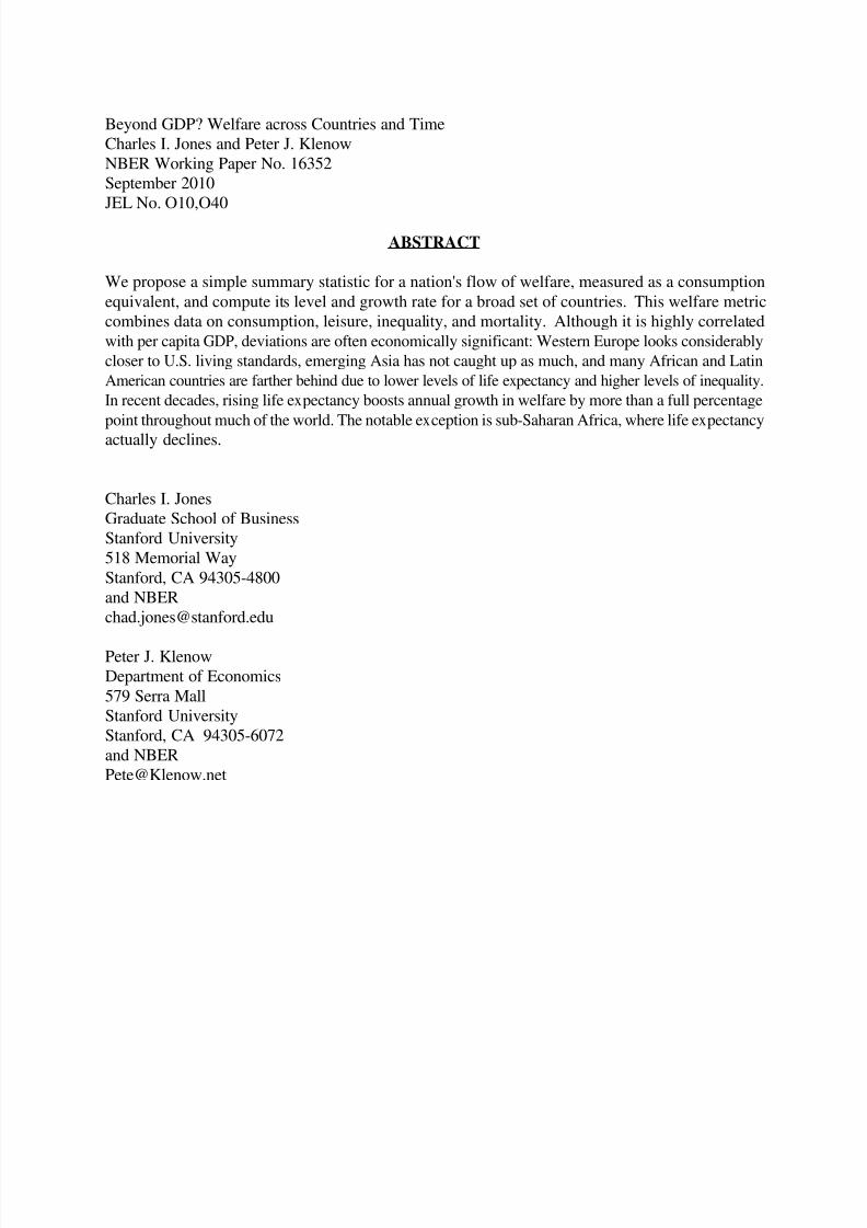
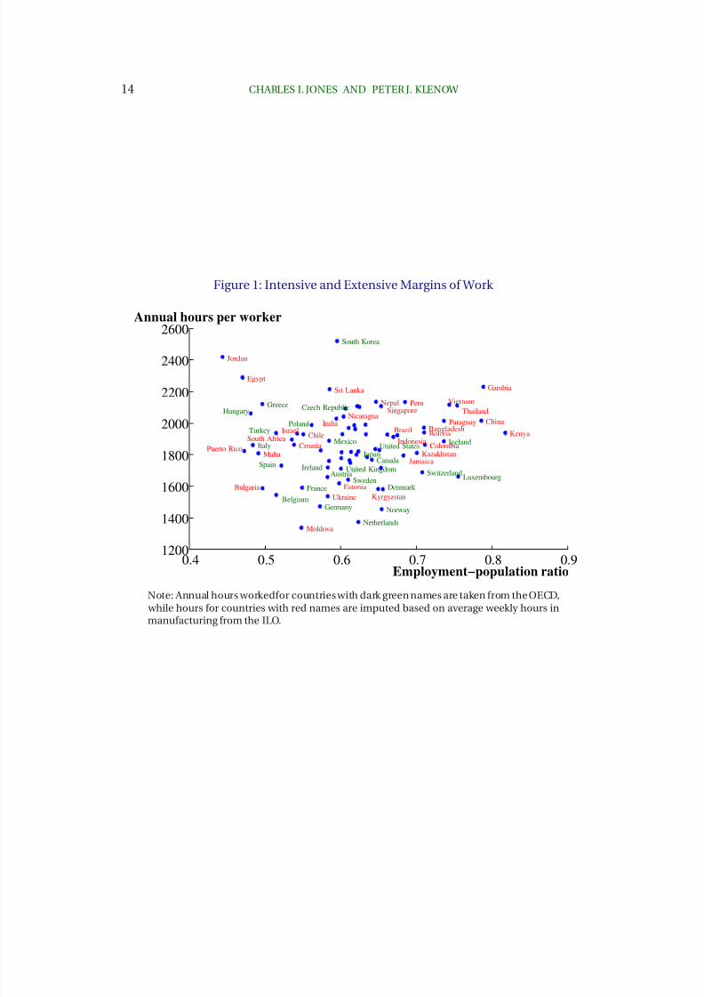
underlying our leisure measure are shown in Figure 1.6
Assuming a time endowment of 16× 365 = 5840 hours per year (sleep is counted
as neither work nor leisure), our measure of ℓ is
ℓ = 1 − annual hours worked per worker
16 × 365· employment
adult population.7
In the United States, the ratio of employment to adult population is 0.65 and average
annual hours worked is 1,836. These values imply that the fraction of time devoted
to leisure and home production is just under 80%. Germany has one of the highest
values of ℓ in our data. Its employment-population ratio is 0.57 and average annual
hours worked is only 1,473, so that the leisure fraction of the time endowment is
86%. To see why these basic numbers are so high, notice that workers, who are only
about half the population, usually devote more than 2/3 of their time endowment
to leisure, so leisure and home production are pretty high everywhere and vary by
less than one might have thought.
6Parente, Rogerson and Wright (2000) argue that barriers to capital accumulation explain some of this variationin market hours worked. Like us,they emphasize thegain in home production alongsidethe loss in market output. Like Prescott (2004), Ohanian, Raffo and Rogerson (2008) attribute some of the OECD differences to tax rates.
7Dividing by the adult population imposes the assumption that adults and children have the sameamount of leisure on average (e.g. because of schooling or child labor). An alternative of treating children’s time as entirely leisure does not change our key points.
8/2/2019 Beyond GDP Welfare
http://slidepdf.com/reader/full/beyond-gdp-welfare 15/55
14 CHARLES I. JONES AND PETER J. KLENOW
Figure 1: Intensive and Extensive Margins of Work
0.4 0.5 0.6 0.7 0.8 0.91200
1400
1600
1800
2000
2200
2400
2600
Austria
Belgium
Canada
Czech Republic
Denmark France
Germany
GreeceHungary
Iceland
Ireland
ItalyJapan
South Korea
Luxembourg
Mexico
Netherlands
Norway
Poland
Spain
SwedenSwitzerland
Turkey
United Kingdom
United States
BangladeshBolivia
Brazil
Bulgaria
Chile
China
ColombiaCroatia
Egypt
Estonia
Gambia
India
Indonesia
Israel
Jamaica
Jordan
Kazakhstan
Kenya
Kyrgyzstan
Malta
Moldova
Nepal
NicaraguaParaguay
Peru
Puerto Rico
Singapore
South Africa
Sri Lanka
Thailand
Ukraine
Vietnam
Employment−population ratio
Annual hours per worker
Note: Annual hours workedfor countries with dark green names are taken from the OECD, while hours for countries with red names are imputed based on average weekly hours inmanufacturing from the ILO.
8/2/2019 Beyond GDP Welfare
http://slidepdf.com/reader/full/beyond-gdp-welfare 16/55
WELFARE ACROSS COUNTRIES AND TIME 15
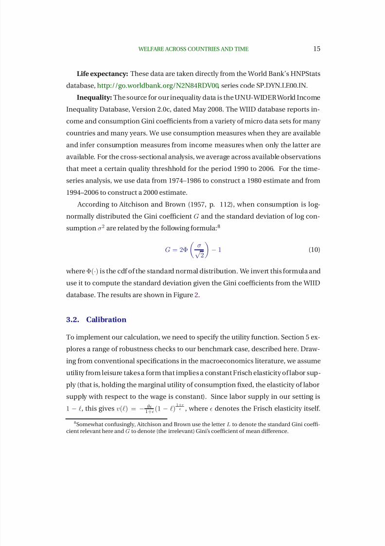
Life expectancy: These data are taken directly from the World Bank’s HNPStats
database, http://go.worldbank.org/N2N84RDV00, series code SP.DYN.LE00.IN.
Inequality: The source for our inequality data is the UNU-WIDER World Income
Inequality Database, Version 2.0c, dated May 2008. The WIID database reports in-
come and consumption Gini coefficients from a variety of micro data sets for many
countries and many years. We use consumption measures when they are available
and infer consumption measures from income measures when only the latter are
available. For the cross-sectional analysis, we average across available observations
that meet a certain quality threshhold for the period 1990 to 2006. For the time-
series analysis, we use data from 1974–1986 to construct a 1980 estimate and from
1994–2006 to construct a 2000 estimate.
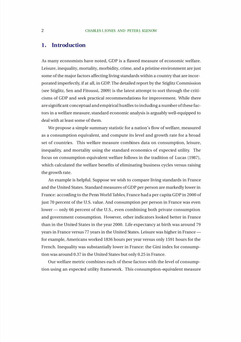
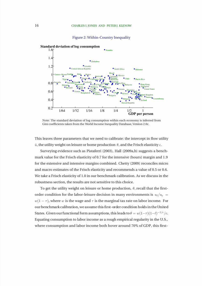
According to Aitchison and Brown (1957, p. 112), when consumption is log-
normally distributed the Gini coefficient G and the standard deviation of log con-
sumption σ2 are related by the following formula:8
G = 2Φ
σ√
2
− 1 (10)
where Φ(·) is the cdf of the standard normal distribution. We invert this formula and
use it to compute the standard deviation given the Gini coefficients from the WIID
database. The results are shown in Figure 2.
3.2. Calibration
To implement our calculation, we need to specify the utility function. Section 5 ex-
plores a range of robustness checks to our benchmark case, described here. Draw-
ing from conventional specifications in the macroeconomics literature, we assume
utility from leisure takes a form that implies a constant Frisch elasticity of labor sup-
ply (that is, holding the marginal utility of consumption fixed, the elasticity of labor
supply with respect to the wage is constant). Since labor supply in our setting is
1 − ℓ, this gives v(ℓ) = − θǫ1+ǫ(1 − ℓ)
1+ǫǫ , where ǫ denotes the Frisch elasticity itself.
8Somewhat confusingly, Aitchison and Brown use the letter L to denote the standard Gini coeffi-cient relevant here and G to denote (the irrelevant) Gini’s coefficient of mean difference.
8/2/2019 Beyond GDP Welfare
http://slidepdf.com/reader/full/beyond-gdp-welfare 17/55
16 CHARLES I. JONES AND PETER J. KLENOW
Figure 2: Within-Country Inequality
1/64 1/32 1/16 1/8 1/4 1/2 10.2
0.4
0.6
0.8
1
1.2
1.4
1.6
Albania
Bahamas
Bangladesh Belarus
Benin
Bolivia
Botswana
Brazil
Bulgaria
Burundi
Cambodia
Cameroon
Central African Republic
ChileChina
Colombia
Costa RicaCote d‘Ivoire
Djibouti
Estonia
Ethiopia
GeorgiaGhana
Greece
Guinea−Bissau Haiti
Hong Kong
Iceland
India Israel
Jordan
Kenya
Latvia
Lesotho
Luxembourg
MalaysiaMauritania
Mauritius
Mexico
Moldova
Namibia
NigerNigeria
Norway
Pakistan
PanamaPuerto Rico
Singapore
Slovak Republic
Somalia
South Africa
Spain
Sweden
TanzaniaThailandUganda
United Kingdom
United StatesVietnam
Yemen
Zambia
Zimbabwe
GDP per person
Standard deviation of log consumption
Hungary
Japan
Note: The standard deviation of log consumption within each economy is inferred fromGini coefficients taken from the World Income Inequality Database, Version 2.0c.
This leaves three parameters that we need to calibrate: the intercept in flow utility
u, the utility weight on leisure or home production θ, and the Frisch elasticity ǫ.
Surveying evidence such as Pistaferri (2003), Hall (2009a,b) suggests a bench-
mark value for the Frisch elasticity of 0.7 for the intensive (hours) margin and 1.9
for the extensive and intensive margins combined. Chetty (2009) reconciles micro
and macro estimates of the Frisch elasticity and recommends a value of 0.5 or 0.6.
We take a Frisch elasticity of 1.0 in our benchmark calibration. As we discuss in the
robustness section, the results are not sensitive to this choice.
To get the utility weight on leisure or home production, θ, recall that the first-
order condition for the labor-leisure decision in many environments is uℓ/uc =
w(1 − τ ), where w is the wage and τ is the marginal tax rate on labor income. For
our benchmark calibration, we assume this first-order condition holds in the United
States. Given our functional form assumptions, this leads to θ = w(1−τ )(1−ℓ)−1/ǫ/c.
Equating consumption to labor income as a rough empirical regularity in the U.S.,
where consumption and labor income both hover around 70% of GDP, this first-
8/2/2019 Beyond GDP Welfare
http://slidepdf.com/reader/full/beyond-gdp-welfare 18/55
WELFARE ACROSS COUNTRIES AND TIME 17
order condition implies θ = (1 − τ )(1 − ℓ)−1+ǫǫ . We take the (average) marginal tax
rate in the United States from Barro and Redlick (2009), who report a value of 0.387
for 1998–2002, consistent with the 40 percent rate used by Prescott (2004). Since
ℓus = .7970 in our data, our benchmark case sets θ = 14.883.
Calibration of the intercept in flow utility, u, is less familiar. The value of this pa-
rameter matters because of the role played by life expectancy: additional life means
more periods of flow utility, so the level of flow utility is key to valuing differences in
life expectancy. We choose u so that a 40-year old in the United States in 2000 has a
value of remaining life equal to $4 million in 2000 prices. In their survey of the liter-
ature, Viscusi and Aldy (2003) recommend values in the range of $5.5–$7.5 million.
Murphy and Topel (2006) choose a value of around $6 million. At the other end of
the spectrum, Ashenfelter and Greenstone (2004) support much lower values, less
than $2 million. Our baseline value of $4 million is broadly consistent with this lit-
erature. This choice leads to u = 5.5441 when consumption in the United States
is normalized to 1 in the year 2000 and leisure is set equal to its observed value of
0.7970.9
4. Standards of Living: the Macro Calculation
We now carry out consumption-equivalent welfare calculations across countries
and over time using the macro data. The calculation across countries is the quan-
titative implementation of equation (7). The calculation over time will be for the
growth rate version of this expression, equation (9). More exactly, we average these
equivalent variations with the compensating variation analogues. We present our
results in the form of several “key points”.
4.1. Across Countries
9For this exercise, we use the mortality data by age for the 2000–2005 period from the Human Mor-tality Database, http://www.mortality.org/cgi-bin/hmd/country.php?cntr=USA&level=1. We assumeconsumption grows at a constant annual rate of 2% as the individual ages.
8/2/2019 Beyond GDP Welfare
http://slidepdf.com/reader/full/beyond-gdp-welfare 19/55
18 CHARLES I. JONES AND PETER J. KLENOW
Key Point 1: GDP per person is an excellent indicator of welfare across the
broad range of countries: the two measures have a correlation of 0.95. Nev-
ertheless, for any given country, the difference between the two measures
can be important. Averaged across 134 countries, the typical deviation is
about 46%.
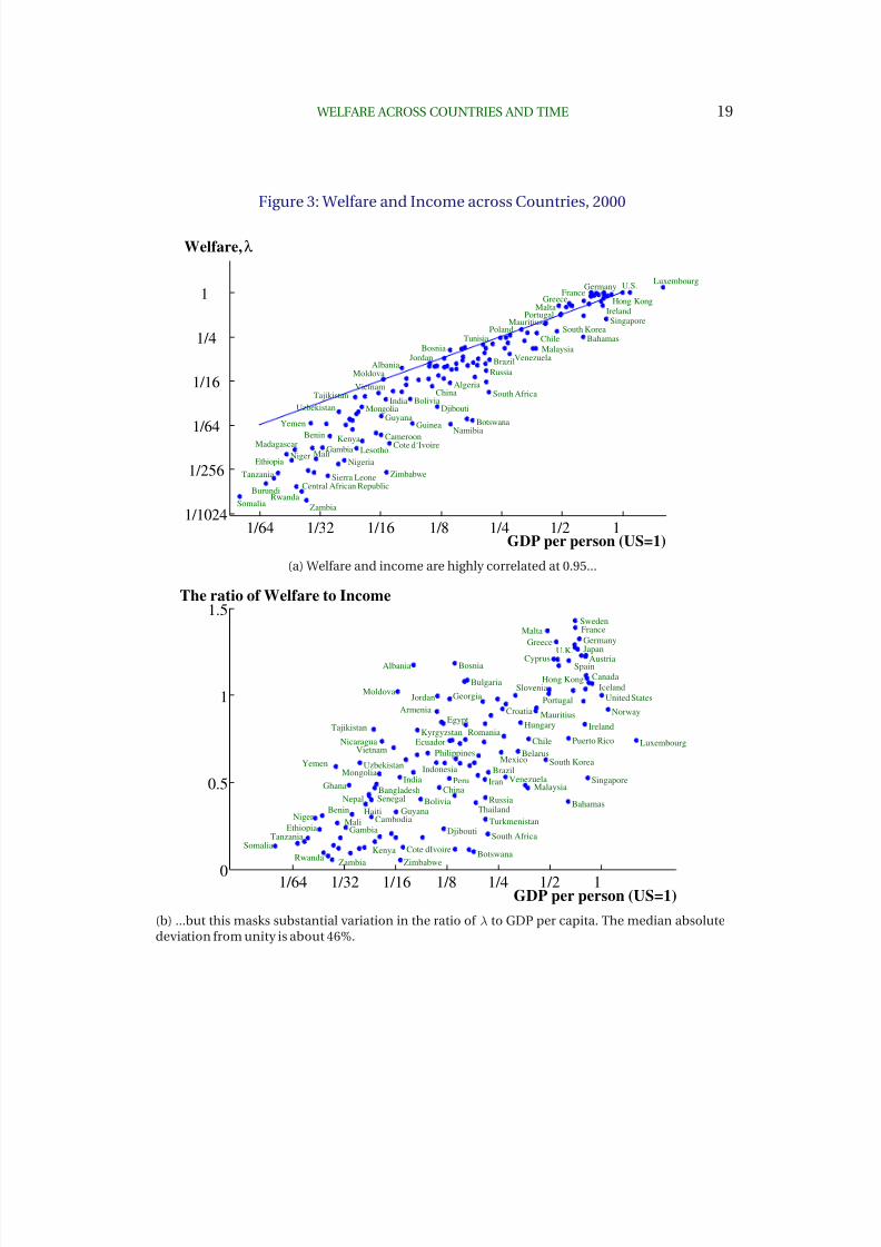
Figure 3 provides a useful overview of our findings for welfare across countries
and illustrates our first point. The top panel plots the welfare measure, λ, against
GDP per person for the year 2000. What emerges prominently from this figure is
that the two measures are extremely highly correlated, with a correlation coefficient
(for the logs) of 0.95. Thus per capita GDP is a good proxy for welfare under our as-
sumptions. At the same time, there are clear departures from the 45-degree line.
In particular, many countries with very low GDP per capita exhibit even lower wel-
fare. As a result, welfare is more dispersed (standard deviation of 1.81 in logs) than
is income (standard deviation of 1.18 in logs).
The bottom panel provides a more revealing look at the deviations. This fig-
ure plots the ratio of welfare to per capita GDP across countries, and here we see
substantial deviations from unity. Countries like France and Sweden have welfare
measures that are over 30% higher than their income. At the other end of the spec-
trum, China and Singapore have welfares that are about half their incomes, while
Botswana and Zimbabwe have ratios of 10 percent or less. The median absolute
deviation from unity is 0.458 in logs.
Key Point 2: Average Western European living standards appear much closer
to those in the United States when we take into account Europe’s longer life
expectancy, additional leisure time, and lower levels of inequality.
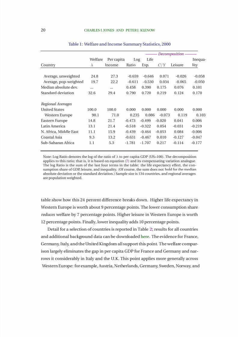
Table 1 presents summary statistics for our welfare decomposition. Of partic-
ular interest at the moment are the regional averages. Per capita GDP in Western
Europe is 71% of that in the United States. Welfare, in contrast, is 90% of the U.S.
value, higher on average by about 24 log points (which we will often call “percent”
or “percentage points” in the remainder of this paper). The last four columns of the
8/2/2019 Beyond GDP Welfare
http://slidepdf.com/reader/full/beyond-gdp-welfare 20/55
WELFARE ACROSS COUNTRIES AND TIME 19
Figure 3: Welfare and Income across Countries, 2000
1/64 1/32 1/16 1/8 1/4 1/2 11/1024
1/256
1/64
1/16
1/4
1
Albania
Algeria
Bahamas
Benin
Bolivia
Bosnia
Botswana
Brazil
Burundi
Cameroon
Central African Republic
Chile
China
Cote d‘Ivoire
Djibouti
Ethiopia
France
Gambia
Germany
Greece
GuineaGuyana
Hong Kong
India
Ireland
Jordan
Kenya
South Korea
Lesotho
Luxembourg
Madagascar
Malaysia
Mali
Malta
Mauritius
Moldova
Mongolia
Namibia
NigerNigeria
Poland
Portugal
Russia
Rwanda
Sierra Leone
Singapore
Somalia
South AfricaTajikistan
Tanzania
Tunisia
U.S.
Uzbekistan
Venezuela
Vietnam
Yemen
Zambia
Zimbabwe
GDP per person (US=1)
Welfare,λ
(a) Welfare and income are highly correlated at 0.95...
1/64 1/32 1/16 1/8 1/4 1/2 10
0.5
1
1.5
Albania
Armenia
Austria
Bahamas
Bangladesh
Belarus
BeninBolivia
Bosnia
Botswana
Brazil
Bulgaria
Cambodia
Canada
Chile
China
Cote dIvoire
Croatia
Cyprus
Djibouti
Ecuador
Egypt
Ethiopia
France
Gambia
Georgia
Germany
Ghana
Greece
GuyanaHaiti
Hong Kong
Hungary
Iceland
India
Indonesia
Iran
Ireland
Japan
Jordan
Kenya
South Korea
Kyrgyzstan
Luxembourg
Malaysia
Mali
Malta
Mauritius
Mexico
Moldova
Mongolia
Nepal
Nicaragua
Niger
Norway
Peru
Philippines
Portugal
Puerto RicoRomania
Russia
Rwanda
Senegal
Singapore
Slovenia
SomaliaSouth Africa
Spain
Sweden
Tajikistan
Tanzania
Thailand
Turkmenistan
U.K.
United States
Uzbekistan
Venezuela
Vietnam
Yemen
Zambia Zimbabwe
GDP per person (US=1)
The ratio of Welfare to Income
(b) ...but this masks substantial variation in the ratio of λ to GDP per capita. The median absolutedeviation from unity is about 46%.
8/2/2019 Beyond GDP Welfare
http://slidepdf.com/reader/full/beyond-gdp-welfare 21/55
20 CHARLES I. JONES AND PETER J. KLENOW
Table 1: Welfare and Income Summary Statistics, 2000
——— Decomposition ———
Welfare Per capita Log Life Inequa-Country λ Income Ratio Exp. C/Y Leisure lity
Average, unweighted 24.8 27.3 -0.659 -0.646 0.071 -0.026 -0.058
Average, pop-weighted 19.7 22.2 -0.611 - 0.530 0.034 -0.065 -0.050
Median absolute dev. ... ... 0.458 0.390 0.175 0.076 0.101
Standard deviation 32.6 29.4 0.790 0.720 0.219 0.124 0.170
Regional Averages
United States 100.0 100.0 0.000 0.000 0.000 0.000 0.000
Western Europe 90.1 71.0 0.235 0.086 -0.073 0.119 0.103
Eastern Europe 14.8 21.7 -0.473 -0.499 -0.020 0.041 0.006
Latin America 13.1 21.4 -0.518 -0.322 0.054 -0.031 -0.219
N. Africa, Middle East 11.1 15.9 -0.439 -0.464 -0.053 0.084 -0.006
Coastal Asia 9.3 13.2 -0.631 -0.467 0.010 -0.127 -0.047
Sub-Saharan Africa 1.1 5.3 -1.781 -1.707 0.217 -0.114 -0.177
Note: Log Ratio denotes the log of the ratio of λ to per capita GDP (US=100). The decompositionapplies to this ratio; that is, it is based on equation (7) and its compensating variation analogue.The log Ratio is the sum of the last four terms in the table: the life expectancy effect, the con-sumption share of GDP, leisure, and inequality. (Of course, the sum does not hold for the medianabsolute deviation or the standard deviation.) Sample size is 134 countries, and regional averages
are population weighted.
table show how this 24 percent difference breaks down. Higher life expectancy in
Western Europe is worth about 9 percentage points. The lower consumption share
reduces welfare by 7 percentage points. Higher leisure in Western Europe is worth
12 percentage points. Finally, lower inequality adds 10 percentage points.
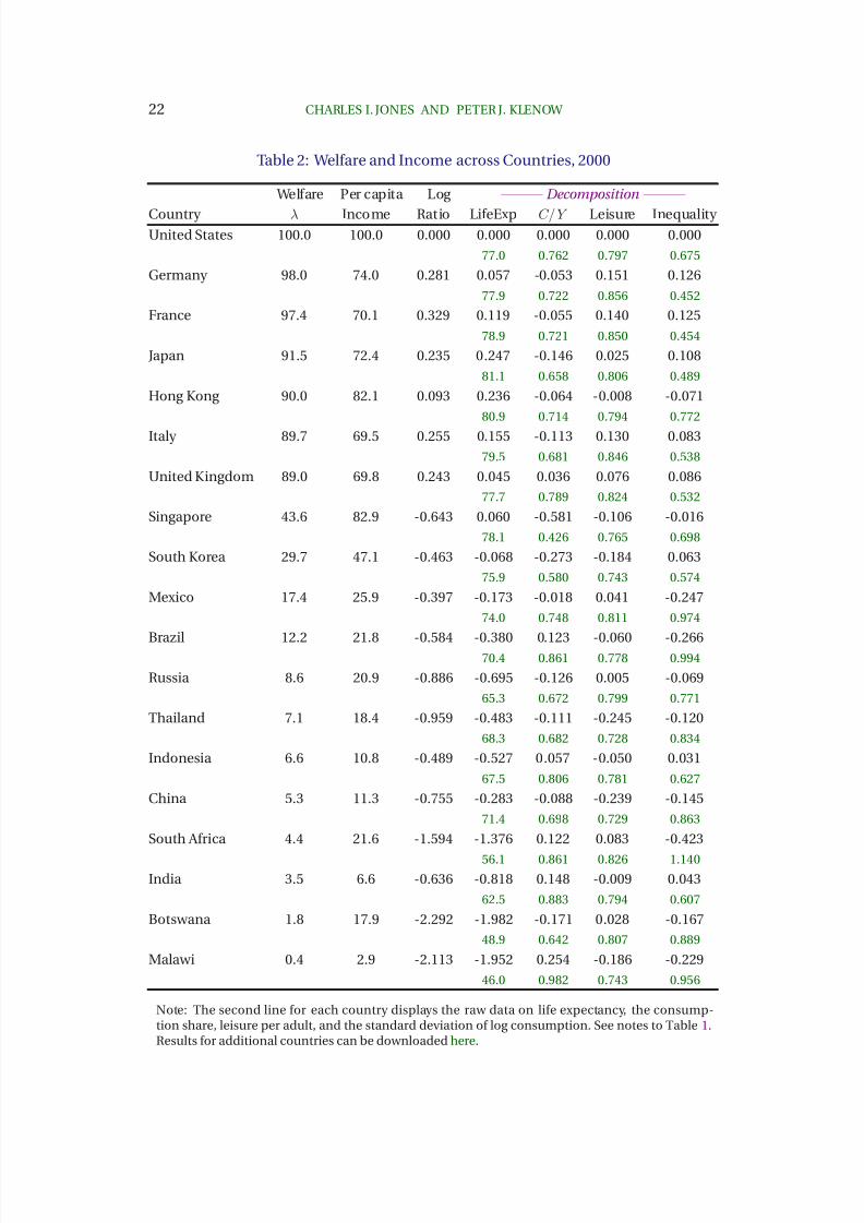
Detail for a selection of countries is reported in Table 2; results for all countries
and additional background data can be downloaded here. The evidence for France,
Germany, Italy, and the United Kingdom all support this point. The welfare compar-
ison largely eliminates the gap in per capita GDP for France and Germany and nar-
rows it considerably in Italy and the U.K. This point applies more generally across
Western Europe: for example, Austria, Netherlands, Germany, Sweden, Norway, and
8/2/2019 Beyond GDP Welfare
http://slidepdf.com/reader/full/beyond-gdp-welfare 22/55
WELFARE ACROSS COUNTRIES AND TIME 21
Luxembourg all end up with even higher welfare than France.
Differences between welfare and income are also quite stark for East Asia, as
shown in the middle rows of Table 2. According to GDP per person, Singapore and
Hong Kong are close to U.S. income, at about 82%. The welfare measure substan-
tially alters this picture. Hong Kong registers at 90% of U.S. welfare, while Singapore
falls to 44%. A similar decline occurs in South Korea, from 47% in income to 30% in
welfare. Both countries, and Japan as well, see their welfare limited sharply by their
well-known low consumption shares. This force is largest for Singapore, where the
consumption share of GDP is substantially below 0.5. This is the levels-analog of
Alwyn Young’s (1992) growth accounting point, of course. Singapore has sustained
a very high investment rate in recent decades. This capital accumulation raises in-
come and consumption in the long run, but the effect on consumption is less than
the effect on income, which reduces the welfare-income ratio. Similarly, leisure is
low in Singapore and South Korea, also reducing welfare for a given level of income.
Working hard and investing for the future are well-established means for raising
GDP. Nevertheless, these approaches have costs that are not reflected in GDP itself.
Key Point 3: Many developing countries — including much of sub-Saharan
Africa, Latin America, southern Asia, and China — are poorer than incomessuggest because of a combination of shorter lives and extreme inequality.
This point can be seen clearly in the regional averages for sub-Saharan Africa
and Latin America at the bottom of Table 1. Countries in sub-Saharan Africa have
welfare that is only about 1% of the U.S. level, much lower than their 5% relative
income, largely because of very low life expectancy. In Latin America, lower life
expectancy and higher inequality combine to hold their welfare down to 13% of the
U.S. level on average, vs. 21% of U.S. income.
The details for a number of countries are reported in the lower half of Table 2,
where the same story appears repeatedly. A life expectancy of only 65 years cuts
Russia’s welfare by nearly 70 percent. Massive inequality in Brazil (a standard de-
viation of log consumption of 0.99) lowers welfare by 27 percent. China is at 11%
of U.S. per capita income in 2000, but only about 5% of U.S. welfare. China suffers
8/2/2019 Beyond GDP Welfare
http://slidepdf.com/reader/full/beyond-gdp-welfare 23/55
22 CHARLES I. JONES AND PETER J. KLENOW
Table 2: Welfare and Income across Countries, 2000
Welfare Per capita Log ——— Decomposition ———
Country λ Income Ratio LifeExp C/Y Leisure Inequality United States 100.0 100.0 0.000 0.000 0.000 0.000 0.000
77.0 0.762 0.797 0.675
Germany 98.0 74.0 0.281 0.057 -0.053 0.151 0.126
77.9 0.722 0.856 0.452
France 97.4 70.1 0.329 0.119 -0.055 0.140 0.125
78.9 0.721 0.850 0.454
Japan 91.5 72.4 0.235 0.247 -0.146 0.025 0.108
81.1 0.658 0.806 0.489
Hong Kong 90.0 82.1 0.093 0.236 -0.064 -0.008 -0.071
80.9 0.714 0.794 0.772
Italy 89.7 69.5 0.255 0.155 -0.113 0.130 0.083
79.5 0.681 0.846 0.538
United Kingdom 89.0 69.8 0.243 0.045 0.036 0.076 0.086
77.7 0.789 0.824 0.532
Singapore 43.6 82.9 -0.643 0.060 -0.581 -0.106 -0.016
78.1 0.426 0.765 0.698
South Korea 29.7 47.1 -0.463 -0.068 -0.273 -0.184 0.063
75.9 0.580 0.743 0.574
Mexico 17.4 25.9 -0.397 -0.173 -0.018 0.041 -0.247
74.0 0.748 0.811 0.974
Brazil 12.2 21.8 -0.584 -0.380 0.123 -0.060 -0.26670.4 0.861 0.778 0.994
Russia 8.6 20.9 -0.886 -0.695 -0.126 0.005 -0.069
65.3 0.672 0.799 0.771
Thailand 7.1 18.4 -0.959 -0.483 -0.111 -0.245 -0.120
68.3 0.682 0.728 0.834
Indonesia 6.6 10.8 -0.489 -0.527 0.057 -0.050 0.031
67.5 0.806 0.781 0.627
China 5.3 11.3 -0.755 -0.283 -0.088 -0.239 -0.145
71.4 0.698 0.729 0.863
South Africa 4.4 21.6 -1.594 -1.376 0.122 0.083 -0.423
56.1 0.861 0.826 1.140
India 3.5 6.6 -0.636 -0.818 0.148 -0.009 0.043
62.5 0.883 0.794 0.607
Botswana 1.8 17.9 -2.292 -1.982 -0.171 0.028 -0.167
48.9 0.642 0.807 0.889
Malawi 0.4 2.9 -2.113 -1.952 0.254 -0.186 -0.229
46.0 0.982 0.743 0.956
Note: The second line for each country displays the raw data on life expectancy, the consump-tion share, leisure per adult, and the standard deviation of log consumption. See notes to Table 1.Results for additional countries can be downloaded here.
8/2/2019 Beyond GDP Welfare
http://slidepdf.com/reader/full/beyond-gdp-welfare 24/55
WELFARE ACROSS COUNTRIES AND TIME 23
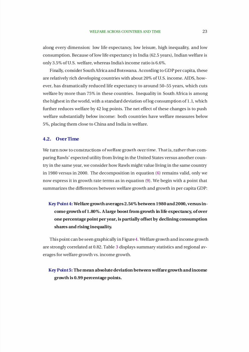
along every dimension: low life expectancy, low leisure, high inequality, and low
consumption. Because of low life expectancy in India (62.5 years), Indian welfare is
only 3.5% of U.S. welfare, whereas India’s income ratio is 6.6%.
Finally, consider South Africa and Botswana. According to GDP per capita, these
are relatively rich developing countries with about 20% of U.S. income. AIDS, how-
ever, has dramatically reduced life expectancy to around 50–55 years, which cuts
welfare by more than 75% in these countries. Inequality in South Africa is among
the highest in the world, with a standard deviation of log consumption of 1.1, which
further reduces welfare by 42 log points. The net effect of these changes is to push
welfare substantially below income: both countries have welfare measures below
5%, placing them close to China and India in welfare.
4.2. Over Time
We turn now to constructions of welfare growth over time. That is, rather than com-
paring Rawls’ expected utility from living in the United States versus another coun-
try in the same year, we consider how Rawls might value living in the same country
in 1980 versus in 2000. The decomposition in equation (6) remains valid, only we
now express it in growth rate terms as in equation (9). We begin with a point that
summarizes the differences between welfare growth and growth in per capita GDP:
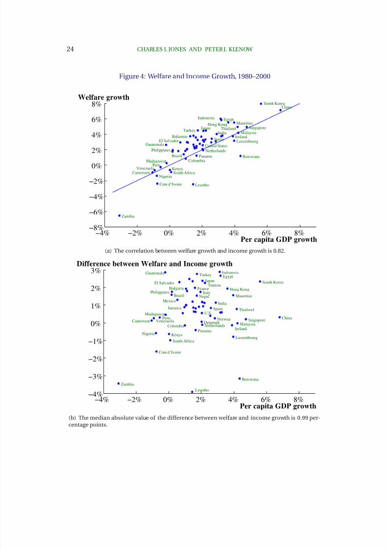
Key Point 4: Welfare growth averages 2.54% between 1980 and 2000, versus in-
come growth of 1.80%. A large boost from growth in life expectancy, of over
one percentage point per year, is partially offset by declining consumption
shares and rising inequality.
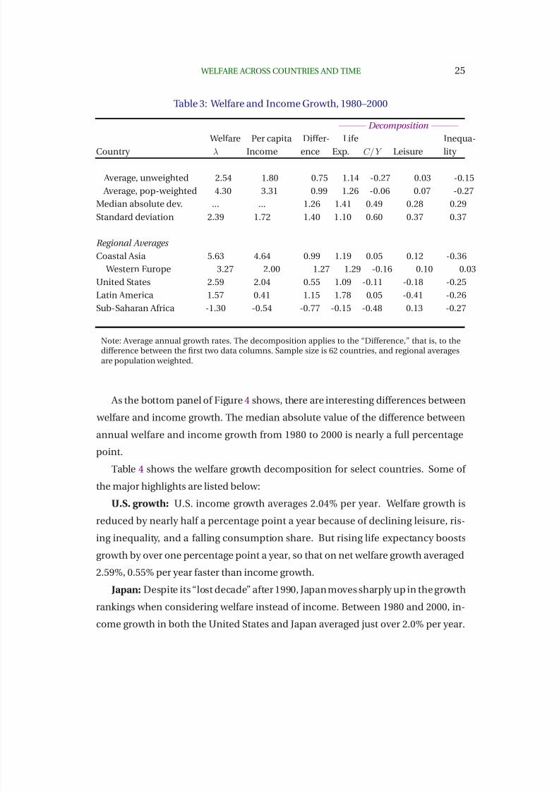
This point can be seen graphically in Figure 4. Welfare growth and income growth
are strongly correlated at 0.82. Table 3 displays summary statistics and regional av-
erages for welfare growth vs. income growth.
Key Point 5: The mean absolute deviation between welfare growth and income
growth is 0.99 percentage points.
8/2/2019 Beyond GDP Welfare
http://slidepdf.com/reader/full/beyond-gdp-welfare 25/55
24 CHARLES I. JONES AND PETER J. KLENOW
Figure 4: Welfare and Income Growth, 1980–2000
−4% −2% 0% 2% 4% 6% 8%−8%
−6%
−4%
−2%
0%
2%
4%
6%
8%
Bahamas
BotswanaBrazil
Cameroon
China
Colombia
Cote d‘Ivoire
Egypt
El SalvadorGuatemala
Hong Kong
India
Indonesia
Ireland
Japan
Kenya
South Korea
Lesotho
Luxembourg
Madagascar
Malaysia
Mauritius
Netherlands
Nigeria
Panama
Peru
Philippines
Singapore
South Africa
Spain
ThailandTurkey
United States
Venezuela
Zambia
Per capita GDP growth
Welfare growth
(a) The correlation between welfare growth and income growth is 0.82.
−4% −2% 0% 2% 4% 6% 8%−4%
−3%
−2%
−1%
0%
1%
2%
3%
Botswana
Brazil
Bulgaria
CameroonChina
Colombia
Cote d‘Ivoire
Denmark
Egypt
El Salvador
France
Guatemala
Hong Kong
India
Indonesia
Ireland
Italy
Jamaica
Japan
Kenya
South Korea
Lesotho
Luxembourg
Madagascar
Malaysia
Mauritius
MexicoNepal
Netherlands
Nigeria
Norway
Panama
Peru
Philippines
Singapore
South Africa
Spain Thailand
Tunisia
Turkey
U.S.
Venezuela
Zambia
Per capita GDP growth
Difference between Welfare and Income growth
(b) The median absolute value of the difference between welfare and income growth is 0.99 per-centage points.
8/2/2019 Beyond GDP Welfare
http://slidepdf.com/reader/full/beyond-gdp-welfare 26/55
WELFARE ACROSS COUNTRIES AND TIME 25
Table 3: Welfare and Income Growth, 1980–2000
——— Decomposition ———
Welfare Per capita Differ- Life Inequa-Country λ Income ence Exp. C/Y Leisure lity
Average, unweighted 2.54 1.80 0.75 1.14 -0.27 0.03 -0.15
Average, pop-weighted 4.30 3.31 0.99 1.26 -0.06 0.07 -0.27
Median absolute dev. ... ... 1.26 1.41 0.49 0.28 0.29
Standard deviation 2.39 1.72 1.40 1.10 0.60 0.37 0.37
Regional Averages
Coastal Asia 5.63 4.64 0.99 1.19 0.05 0.12 -0.36
Western Europe 3.27 2.00 1.27 1.29 -0.16 0.10 0.03
United States 2.59 2.04 0.55 1.09 -0.11 -0.18 -0.25
Latin America 1.57 0.41 1.15 1.78 0.05 -0.41 -0.26
Sub-Saharan Africa -1.30 -0.54 -0.77 -0.15 -0.48 0.13 -0.27
Note: Average annual growth rates. The decomposition applies to the “Difference,” that is, to thedifference between the first two data columns. Sample size is 62 countries, and regional averagesare population weighted.
As the bottom panel of Figure 4 shows, there are interesting differences between
welfare and income growth. The median absolute value of the difference between
annual welfare and income growth from 1980 to 2000 is nearly a full percentage
point.
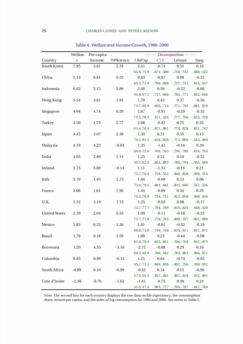
Table 4 shows the welfare growth decomposition for select countries. Some of
the major highlights are listed below:
U.S. growth: U.S. income growth averages 2.04% per year. Welfare growth is
reduced by nearly half a percentage point a year because of declining leisure, ris-
ing inequality, and a falling consumption share. But rising life expectancy boosts
growth by over one percentage point a year, so that on net welfare growth averaged
2.59%, 0.55% per year faster than income growth.
Japan: Despite its “lost decade” after 1990, Japan moves sharply up in the growth
rankings when considering welfare instead of income. Between 1980 and 2000, in-
come growth in both the United States and Japan averaged just over 2.0% per year.
8/2/2019 Beyond GDP Welfare
http://slidepdf.com/reader/full/beyond-gdp-welfare 27/55
26 CHARLES I. JONES AND PETER J. KLENOW
Table 4: Welfare and Income Growth, 1980–2000
Welfare Per capita ——— Decomposition ———
Country λ Income Difference LifeExp C/ Y Leisure Ineq.South Korea 7.95 5.61 2.34 2.41 -0.74 0.51 0.16
65.8, 75.9 .671, .580 .718, .743 .580, .522
China 7.13 6.81 0.32 0.83 -0.07 0.08 -0.52
65.5, 71.4 .708, .698 .727, .731 .443, .637
Indonesia 6.02 3.13 2.89 2.60 0.59 -0.22 -0.08
54.8, 67.5 .717, .806 .784, .771 .622, .648
Hong Kong 5.54 3.61 1.94 1.70 0.42 0.37 -0.56
74.7, 80.9 .656, .714 .771, .794 .681, .829
Singapore 4.94 4.74 0.20 1.67 -0.91 -0.20 -0.35
71.5, 78.1 .511, .426 .777, .766 .622, .726
Turkey 4.50 1.73 2.77 2.08 -0.42 0.75 0.35
61.4, 70.4 .871, .801 .778, .829 .831, .742
Japan 4.45 2.07 2.38 1.39 0.31 0.55 0.13
76.1, 81.1 .618, .658 .771, .806 .543, .494
Malaysia 4.19 4.22 -0.03 1.35 -1.42 -0.16 0.20
66.9, 72.6 .709, .533 .796, .786 .816, .765
India 4.03 2.89 1.14 1.25 0.12 0.10 -0.32
55.7, 62.5 .862, .883 .788, .794 .565, .669
Ireland 3.75 3.89 -0.14 1.11 -1.31 -0.14 0.21
72.7, 76.4 .718, .552 .840, .828 .589, .514
Italy 3.70 1.95 1.75 1.66 -0.09 0.13 0.0673.9, 79.5 .693, .681 .835, .846 .557, .536
France 3.60 1.61 1.98 1.44 -0.09 0.34 0.29
74.2, 78.9 .734, .721 .822, .850 .560, .446
U.K. 3.32 2.19 1.13 1.25 -0.03 0.08 -0.17
73.7, 77.7 .794, .789 .818, .824 .448, .520
United States 2.59 2.04 0.55 1.09 -0.11 -0.18 -0.25
73.7, 77.0 .778, .762 .809, .797 .601, .680
Mexico 1.83 0.53 1.30 1.81 -0.01 -0.32 -0.19
66.8, 74.0 .749, .748 .835, .811 .827, .871
Brazil 1.76 0.18 1.59 1.88 0.23 -0.44 -0.08
62.8, 70.4 .822, .861 .796, .769 .957, .973
Botswana 1.20 4.35 -3.16 -2.72 -0.88 0.29 0.16
60.5, 48.9 .766, .642 .783, .801 .906, .871
Colombia 0.85 0.99 -0.15 1.21 0.04 -0.74 -0.65
65.7, 71.1 .849, .856 .801, .756 .780, .932
South Africa -0.89 0.10 -0.99 -0.32 0.14 0.15 -0.96
57.2, 56.1 .837, .861 .807, .818 .762, .981
Cote d‘Ivoire -2.38 -0.76 -1.62 -1.41 -0.75 0.30 0.24
53.5, 47.4 .903, .777 .769, .787 .847, .788
Note: The second line for each country displays the raw data on life expectancy, the consumption
share, leisure per capita, and the stdev of log consumption for 1980 and 2000. See notes to Table 3.
8/2/2019 Beyond GDP Welfare
http://slidepdf.com/reader/full/beyond-gdp-welfare 28/55
WELFARE ACROSS COUNTRIES AND TIME 27
But increasing life expectancy, a rising consumption share, rising leisure, and falling
inequality more than double Japan’s welfare growth to 4.45% per year, almost two
percentage points faster than U.S. growth over this period. Japan is one of the fastest
growing economies in the world over this period when these additional compo-
nents of welfare are included.
U.S. versus Western Europe: Income growth in the United States and West-
ern Europe is roughly the same, at 2.0%. According to the welfare measure, how-
ever, Western Europe grows more than three-quarters of a percentage point faster
at 3.3%, with life expectancy, leisure, and inequality all contributing to the differ-
ence.
Table 4 illustrates this point for France, Italy, and the United Kingdom. Income
growth in France and Italy was somewhat slower than in the U.S. and U.K. Welfare
growth in all three European countries rises sharply relative to the United States,
however, with all three growing at rates of 3.3% or more. Growth in France more
than doubles, from 1.6% to 3.6%. Life expectancy, leisure, and inequality all con-
tribute to the gain.
China: According to our welfare measure, China is no longer the fastest growing
country in the world from 1980 to 2000. China and South Korea swap places at
the top of the list of fast-growing countries, with growth in South Korea rising to
8.0% and growth in China registering at 7.1%. Chinese welfare growth is slightly
faster than its income growth, but its boost from higher life expectancy is tempered
by rising inequality, which shaves off 0.5 percentage points per year from Chinese
growth. South Korea gains the equivalent of 2.4% faster consumption growth from
its 10 year jump in life expectancy (from 66 to 76).
Latin America: As shown in the regional averages reported in Table 3, Latin
America gains the most of any region of the world from rising life expectancy —
almost 1.8 percentage points. Unfortunately, declines in leisure and rising inequal-
ity offset a third of this gain.
AIDS in Africa: South Africa, Botswana, and Cote d’Ivoire all see their growth
rate reduced sharply by AIDS. In South Africa, declining life expectancy slows growth
by 0.3 percentage points, while rising inequality slows growth by another 1.0 per-
8/2/2019 Beyond GDP Welfare
http://slidepdf.com/reader/full/beyond-gdp-welfare 29/55
28 CHARLES I. JONES AND PETER J. KLENOW
centage point. The net effect is to reduce South Africa’s annual growth from 0.1% to
-0.9%. Young (2005) pointed out that AIDS was a tragedy in Africa but that it might
have beneficial effects on GDP performance by raising the amount of capital per
worker. Our welfare measure provides one way of adding these two components
together to measure the net cost which, as Young suspected, proves to be substan-
tial. Botswana loses the equivalent of 2.7 percentage points of consumption growth
from seeing its life expectancy fall from 60.5 to 48.9 years. Botswana’s growth rate
falls from one of the fastest in the world at 4.35% to well below average at 1.20%.
Already poor sub-Saharan Africa fell further behind the richest countries from 1980
to 2000, and this contrast is magnified by focusing on welfare instead of income.
The new “Singapores”: An important contributor to growth in GDP per person
in many rapidly-growing countries is factor accumulation: increases in the invest-
ment rate and increases in hours worked. This point was emphasized by Young
(1992) in his study of Hong Kong and Singapore. Yet this growth comes at the ex-
pense of current consumption and leisure, so growth in GDP provides an incom-
plete picture of overall economic performance.
Table 4 shows that many of the world’s fastest growing countries are imitating
Singapore in this respect. In terms of welfare growth, Singapore, Malaysia, and
Ireland all lose more than a full percentage point of annual growth to these chan-
nels. Equally interesting, the countries in this list remain among the fastest growing
countries in the world as these negative effects are countered by large gains in life
expectancy.
5. Robustness
Our benchmark results required particular assumptions about the functional form
and parameter values of Rawls’ utility function. Here we gauge the robustness of our
calculations to alternative welfare measures and alternative specifications of utility.
8/2/2019 Beyond GDP Welfare
http://slidepdf.com/reader/full/beyond-gdp-welfare 30/55
WELFARE ACROSS COUNTRIES AND TIME 29
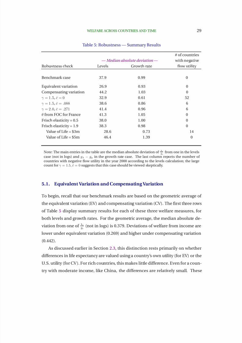
Table 5: Robustness — Summary Results
# of countries
— Median absolute deviation — with negativeRobustness check Levels Growth rate flow utility
Benchmark case 37.9 0.99 0
Equivalent variation 26.9 0.93 0
Compensating variation 44.2 1.03 0
γ = 1.5, c = 0 32.9 0.61 52
γ = 1.5, c = .088 38.6 0.86 6
γ = 2.0, c = .271 41.4 0.96 6
θ from FOC for France 41.3 1.05 0
Frisch elasticity = 0.5 38.0 1.00 0Frisch elasticity = 1.9 38.3 0.98 0
Value of Life = $3m 28.6 0.73 14
Value of Life = $5m 46.4 1.39 0
Note: The main entries in the table are the median absolute deviation of λi
yifrom one in the levels
case (not in logs) and gλ − gy in the growth rate case. The last column reports the number of countries with negative flow utility in the year 2000 according to the levels calculation; the largecount for γ = 1.5, c = 0 suggests that this case should be viewed skeptically.
5.1. Equivalent Variation and Compensating Variation
To begin, recall that our benchmark results are based on the geometric average of
the equivalent variation (EV) and compensating variation (CV). The first three rows
of Table 5 display summary results for each of these three welfare measures, for
both levels and growth rates. For the geometric average, the median absolute de-
viation from one of λiyi (not in logs) is 0.379. Deviations of welfare from income are
lower under equivalent variation (0.269) and higher under compensating variation
(0.442).
As discussed earlier in Section 2.3, this distinction rests primarily on whether
differences in life expectancy are valued using a country’s own utility (for EV) or the
U.S. utility (for CV). For rich countries, this makes little difference. Even for a coun-
try with moderate income, like China, the differences are relatively small. These
8/2/2019 Beyond GDP Welfare
http://slidepdf.com/reader/full/beyond-gdp-welfare 31/55
30 CHARLES I. JONES AND PETER J. KLENOW
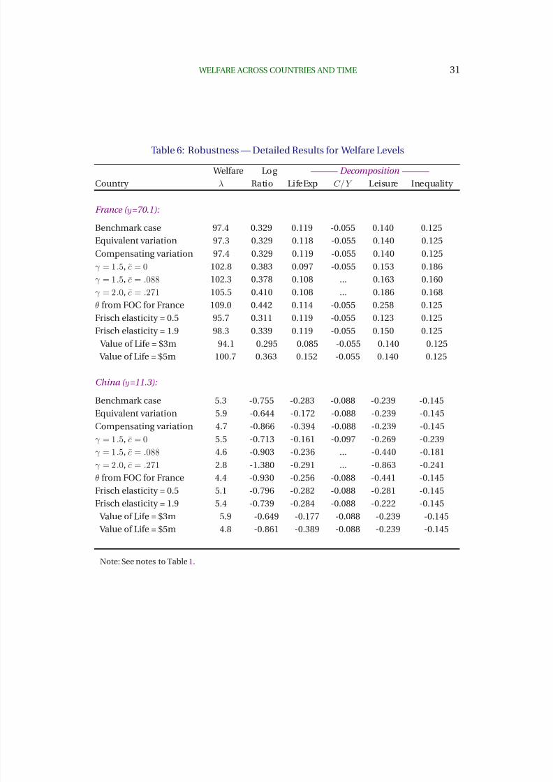
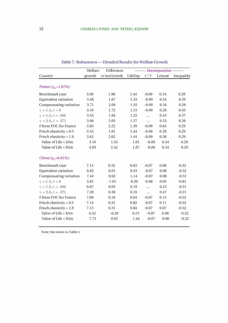
facts are shown in Table 6, which displays our robustness results for two sample
countries, France and China, in levels. (Table 7 does the same for growth rates).
The difference between EV and CV is most apparent for extremely poor coun-
tries. For example, consider Malawi. According to GDP per person, the United
States is 34 times richer than Malawi. Our benchmark welfare measure raises this
ratio to 284. This is the geometric average of an EV ratio of 68 and a CV ratio of 1178.
The factor of 68 comes from an EV approach that puts little value on Malawi’s low
life expectancy: Malawi has such low flow utility that life is not particularly valuable
according to our baseline preference specification. Alternatively, the CV calcula-
tion uses U.S. flow utility to value the shortfall in life expectancy, producing a truly
enormous welfare ratio. The two approaches involve distinct, but arguably equally-
interesting, thought experiments of scaling down U.S. consumption (EV) or scaling
up foreign consumption (CV).
Fortunately, the “key points” we make in this paper are robust to using these
three different welfare measures. This is apparent, for example, in the fact that even
with the EV approach, Malawi is twice as poor as suggested by GDP per person. The
differences only become larger as one moves to our other welfare metrics.
5.2. Alternative Utility Specifications
Our benchmark utility function added log consumption to a leisure term and an in-
tercept. This choice yielded an additive decomposition of welfare differences. Now
consider a more general utility function with non-separable preferences over con-
sumption and leisure:
u(C, ℓ) = u +(C + c)1−γ
1 − γ
1 + (γ − 1)
θǫ
1 + ǫ(1 − ℓ)
1+ǫǫ
γ
− 1
1 − γ . (11)
This functional form reduces to our baseline specification when γ = 1 and c = 0.
In the special case of c = 0, this is the “constant Frisch elasticity” functional form
advocated by Shimer (2009) and Trabandt and Uhlig (2009). The parameter ǫ is the
constant Frisch elasticity of labor supply (the elasticity of time spent working with
respect to the real wage, holding fixed the marginal utility of consumption).
8/2/2019 Beyond GDP Welfare
http://slidepdf.com/reader/full/beyond-gdp-welfare 32/55
WELFARE ACROSS COUNTRIES AND TIME 31
Table 6: Robustness — Detailed Results for Welfare Levels
Welfare Log ——— Decomposition ———
Country λ Ratio LifeExp C/Y Leisure Inequality
France ( y=70.1):
Benchmark case 97.4 0.329 0.119 -0.055 0.140 0.125
Equivalent variation 97.3 0.329 0.118 -0.055 0.140 0.125
Compensating variation 97.4 0.329 0.119 -0.055 0.140 0.125
γ = 1.5, c = 0 102.8 0.383 0.097 -0.055 0.153 0.186
γ = 1.5, c = .088 102.3 0.378 0.108 ... 0.163 0.160
γ = 2.0, c = .271 105.5 0.410 0.108 ... 0.186 0.168
θ from FOC for France 109.0 0.442 0.114 -0.055 0.258 0.125
Frisch elasticity = 0.5 95.7 0.311 0.119 -0.055 0.123 0.125
Frisch elasticity = 1.9 98.3 0.339 0.119 -0.055 0.150 0.125
Value of Life = $3m 94.1 0.295 0.085 -0.055 0.140 0.125
Value of Life = $5m 100.7 0.363 0.152 -0.055 0.140 0.125
China ( y=11.3):
Benchmark case 5.3 -0.755 -0.283 -0.088 -0.239 -0.145
Equivalent variation 5.9 -0.644 -0.172 -0.088 -0.239 -0.145
Compensating variation 4.7 -0.866 -0.394 -0.088 -0.239 -0.145
γ = 1.5, c = 0 5.5 -0.713 -0.161 -0.097 -0.269 -0.239
γ = 1.5, c = .088 4.6 -0.903 -0.236 ... -0.440 -0.181
γ = 2.0, c = .271 2.8 -1.380 -0.291 ... -0.863 -0.241
θ from FOC for France 4.4 -0.930 -0.256 -0.088 -0.441 -0.145
Frisch elasticity = 0.5 5.1 -0.796 -0.282 -0.088 -0.281 -0.145
Frisch elasticity = 1.9 5.4 -0.739 -0.284 -0.088 -0.222 -0.145
Value of Life = $3m 5.9 -0.649 -0.177 -0.088 -0.239 -0.145
Value of Life = $5m 4.8 -0.861 -0.389 -0.088 -0.239 -0.145
Note: See notes to Table 1.
8/2/2019 Beyond GDP Welfare
http://slidepdf.com/reader/full/beyond-gdp-welfare 33/55
8/2/2019 Beyond GDP Welfare
http://slidepdf.com/reader/full/beyond-gdp-welfare 34/55
WELFARE ACROSS COUNTRIES AND TIME 33
Table 5 summarizes a range of robustness checks based on this general form for
preferences. The one sentence summary is that, overall, the results for our bench-
mark case are quite representative and often become even stronger under the vari-
ous alternatives we consider.
Several cases in Table 5 impose more curvature over consumption than in the
log case. With γ = 1.5 , the median absolute deviation from unity for the ratio of
welfare to income falls somewhat to 0.329, down from 0.379 in the baseline case.
Consumption inequality is more costly to Rawls with γ = 1.5 than in our baseline of
γ = 1.
The final column of Table 5, however, reports the number of countries with neg-
ative flow utility in 2000. In the baseline case there are no such countries, which is
reassuring. However, low average consumption, particularly when combined with
high inequality and a high value of γ , can cause expected flow utility for Rawls to
turn negative. Presumably these are not the preferences of individuals living in
these countries. Nearly all of our empirical evidence on utility functions comes from
people with relatively high consumption. Extrapolating these functional forms over
30-fold differences in consumption may be inappropriate, and this could be what
the negative flow utilities among poor countries are signaling. When γ = 1.5 and
c = 0, a remarkable 52 countries exhibit negative expected utility. Obviously, the
plausibility of this particular case is called into question.
Life is presumably very much worth living in all countries. This is why we in-
serted the additional parameter c in our more general utility function. With c > 0,
expected flow utility can remain positive in the presence of lower average consump-
tion and wider consumption inequality. In the fifth row of Table 5 we consider
c = 0.088 along with γ = 1.5. This combination makes Rawls exactly indifferent
between living and dying in Ethiopia, and thus lifts Rawls out of negative territory
in all but 6 countries. This intercept has less impact on expected utility at much
higher levels of consumption (think of adding 8.8% of U.S. consumption to every-
one’s actual consumption in OECD countries). With this combination, income and
welfare differ by slightly more than in the baseline case (0.386 vs. 0.379).
The next row of Table 5 increases curvature further to γ = 2 at the same time
8/2/2019 Beyond GDP Welfare
http://slidepdf.com/reader/full/beyond-gdp-welfare 35/55
34 CHARLES I. JONES AND PETER J. KLENOW
boosting the intercept to c = 0.271 to prevent Rawls from preferring death to life in
many countries. The gaps between welfare and income become even wider.
We next consider a higher weight on leisure vs. consumption in utility. As in the
baseline we have γ = 1 and c = 0, but we now increase the value of θ. In particular,
we choose θ to rationalize the higher choice of average leisure in France rather than
the lower level seen in the U.S. (and use a marginal tax rate of 0.59 for France, taken
from Prescott 2004). As shown in Table 5, increasing the importance of leisure in
this way makes welfare and income differ more, both in levels and growth rates.
Toward the end of Table 5, we consider alternative values for the Frisch elasticity
of labor supply, in particular 0.5 from Chetty (2009) and a high value of 1.9, at the
upper end of Hall’s (2009b) recommendation. These changes have little effect on
our results.
Our final robustness check is to change the intercept in the utility function. We
set the intercept so that the remaining value of life for a 40 year old in the U.S. in
2000 dollars is $3 million or $5 million rather than the baseline value of $4 million.
With a value of life of $3 million in the United States, the intercept in the util-
ity function falls. Life is generally worth less in all countries, so differences in life
expectancy play a smaller role. This reduces the welfare gain from higher longevity
in European countries like France and mitigates the welfare loss in low lifespan de-
veloping countries like China; see Table 6. Overall, the median deviation between
welfare and income falls from our benchmark value of 0.379 to a smaller but still
quite substantial 0.286. Notice that in this case 14 countries exhibit negative ex-
pected utility.
With a U.S. value of life of $5 million, the contrast between welfare and income
is sharper. The deviation between welfare and income rises to 0.464 rather than
0.379 in levels and by 1.40% per year rather than 0.99% per year in 1980–2000 growth
rates. With more surplus to living, differences in the levels and growth rates of life
expectancy naturally matter more to Rawls.
The bottom line of all these variations in the utility specification turns out to
be straightforward: our benchmark results on the contrast between welfare and in-
come hold up quite well in the alternatives we consider.
8/2/2019 Beyond GDP Welfare
http://slidepdf.com/reader/full/beyond-gdp-welfare 36/55
8/2/2019 Beyond GDP Welfare
http://slidepdf.com/reader/full/beyond-gdp-welfare 37/55
8/2/2019 Beyond GDP Welfare
http://slidepdf.com/reader/full/beyond-gdp-welfare 38/55
WELFARE ACROSS COUNTRIES AND TIME 37
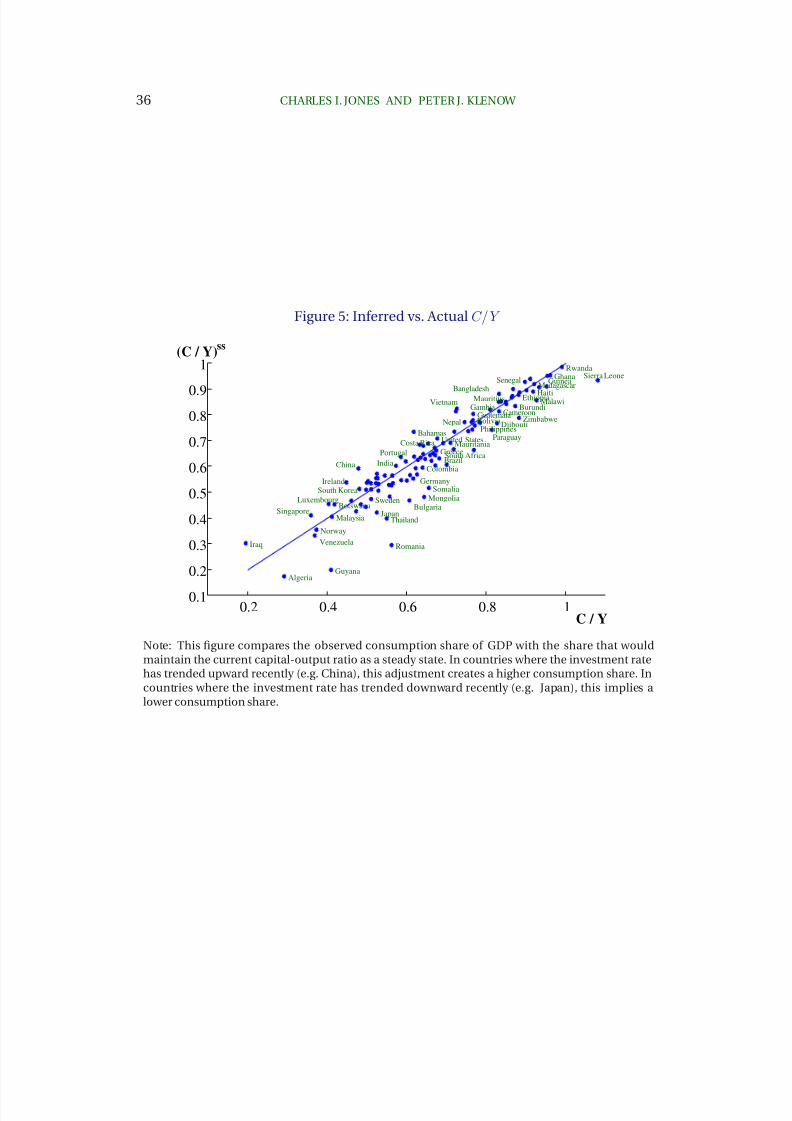
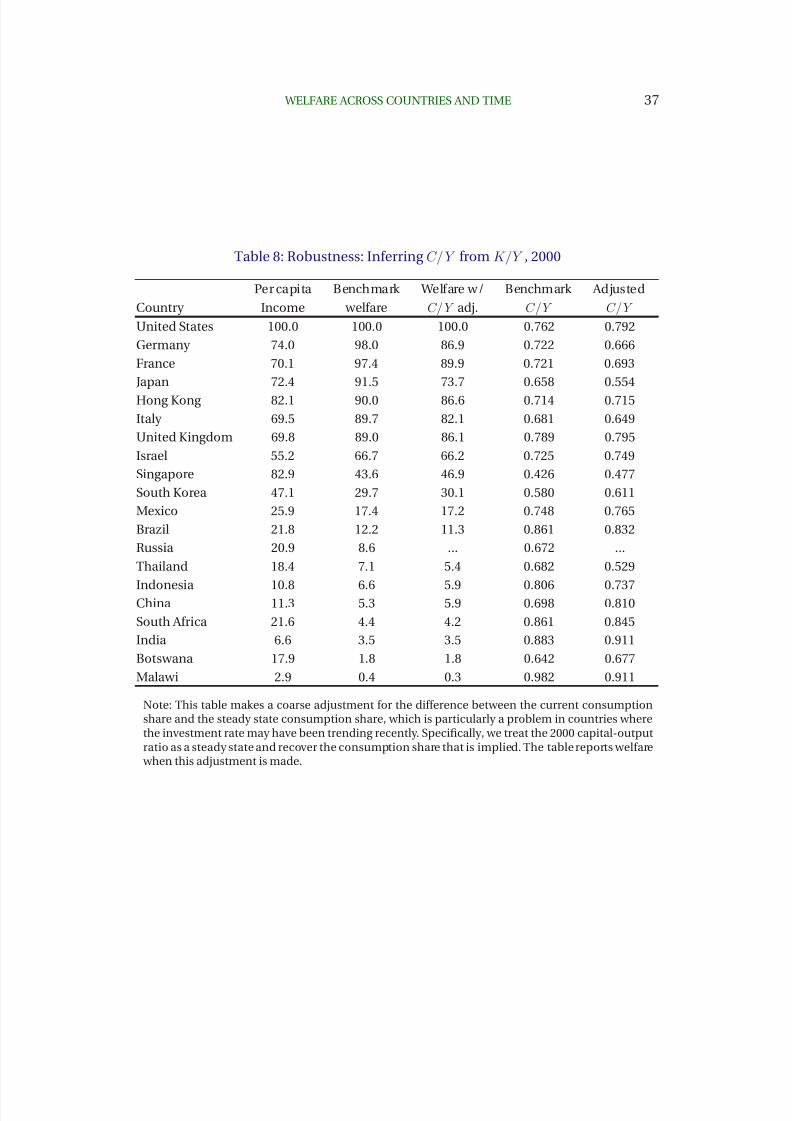
Table 8: Robustness: Inferring C/Y from K/Y , 2000
Per capita Benchmark Welfare w/ Benchmark Adjusted
Country Income welfare C/Y adj. C/Y C/Y
United States 100.0 100.0 100.0 0.762 0.792
Germany 74.0 98.0 86.9 0.722 0.666
France 70.1 97.4 89.9 0.721 0.693
Japan 72.4 91.5 73.7 0.658 0.554
Hong Kong 82.1 90.0 86.6 0.714 0.715
Italy 69.5 89.7 82.1 0.681 0.649
United Kingdom 69.8 89.0 86.1 0.789 0.795
Israel 55.2 66.7 66.2 0.725 0.749
Singapore 82.9 43.6 46.9 0.426 0.477
South Korea 47.1 29.7 30.1 0.580 0.611
Mexico 25.9 17.4 17.2 0.748 0.765
Brazil 21.8 12.2 11.3 0.861 0.832
Russia 20.9 8.6 ... 0.672 ...
Thailand 18.4 7.1 5.4 0.682 0.529
Indonesia 10.8 6.6 5.9 0.806 0.737China 11.3 5.3 5.9 0.698 0.810
South Africa 21.6 4.4 4.2 0.861 0.845
India 6.6 3.5 3.5 0.883 0.911
Botswana 17.9 1.8 1.8 0.642 0.677
Malawi 2.9 0.4 0.3 0.982 0.911
Note: This table makes a coarse adjustment for the difference between the current consumptionshare and the steady state consumption share, which is particularly a problem in countries wherethe investment rate may have been trending recently. Specifically, we treat the 2000 capital-outputratio as a steady state and recover the consumption share that is implied. The table reports welfare when this adjustment is made.
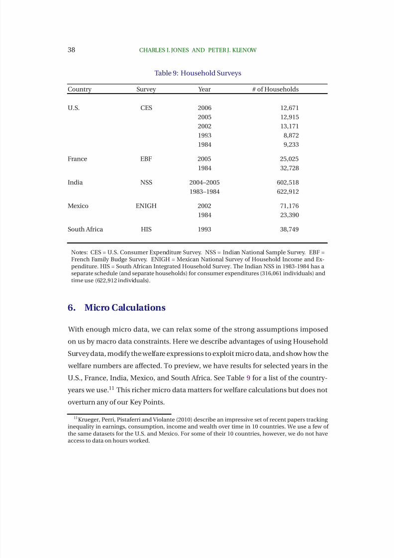
8/2/2019 Beyond GDP Welfare
http://slidepdf.com/reader/full/beyond-gdp-welfare 39/55
38 CHARLES I. JONES AND PETER J. KLENOW
Table 9: Household Surveys
Country Survey Year # of Households
U.S. CES 2006 12,671
2005 12,915
2002 13,171
1993 8,872
1984 9,233
France EBF 2005 25,025
1984 32,728
India NSS 2004–2005 602,518
1983–1984 622,912
Mexico ENIGH 2002 71,176
1984 23,390
South Africa HIS 1993 38,749
Notes: CES = U.S. Consumer Expenditure Survey. NSS = Indian National Sample Survey. EBF =French Family Budge Survey. ENIGH = Mexican National Survey of Household Income and Ex-penditure. HIS = South African Integrated Household Survey. The Indian NSS in 1983-1984 has aseparate schedule (and separate households) for consumer expenditures (316,061 individuals) andtime use (622,912 individuals).
6. Micro Calculations
With enough micro data, we can relax some of the strong assumptions imposed
on us by macro data constraints. Here we describe advantages of using Household
Survey data, modify the welfare expressions to exploit micro data, and show how the
welfare numbers are affected. To preview, we have results for selected years in the
U.S., France, India, Mexico, and South Africa. See Table 9 for a list of the country-
years we use.11
This richer micro data matters for welfare calculations but does notoverturn any of our Key Points.
11Krueger, Perri, Pistaferri and Violante (2010) describe an impressive set of recent papers tracking inequality in earnings, consumption, income and wealth over time in 10 countries. We use a few of the same datasets for the U.S. and Mexico. For some of their 10 countries, however, we do not haveaccess to data on hours worked.
8/2/2019 Beyond GDP Welfare
http://slidepdf.com/reader/full/beyond-gdp-welfare 40/55
WELFARE ACROSS COUNTRIES AND TIME 39
6.1. Advantages of Micro Data
Recall that, for a number of countries (especially developed ones), the Gini coef-
ficients are based on income rather than consumption. Household Surveys con-
taining data on consumption expenditures enable us to calculate consumption in-
equality directly rather than inferring it from income inequality.
With micro data, furthermore, we can allow for an arbitrary distribution of con-
sumption instead of assuming a log-normal distribution. As empirical income and
wealth distributions often feature long right tails, this flexibility could be crucial for
measuring the welfare costs of inequality.12
With household-level data we can be more confident that consumption is de-
fined consistently across countries and time. For every country we exclude expendi-
tures on durable goods and focus on nondurable expenditures inclusive of services
(such as rent and owner-occupied housing).13
In all cases, the micro datasets we use include the reported age composition of
each household. We allocate consumption to each household member — so far
equally (i.e., per capita), although we could alternatively use an adult-equivalent
definition or allocate a higher fraction of consumption to adults. By allocating ex-
penditures to individuals we presumably get a better measure of inequality within
countries, for example if poorer households tend to be larger. We can take into ac-
count household size and age composition in a way the Gini coefficients do not.
The household surveys we analyze include information related to hours worked
for the adults and at least older children in the household. For the children be-
low the age covered in the survey (12 Mexico, 16 in France and South Africa), we
assume zero hours worked. Importantly, the surveys ask about time spent in self-
employment, including subsistence agriculture.
As with consumption, having leisure by age allows us to deal with differences in
the age composition of the population across countries and time. Moreover, we can
12Top-coding does not occur for consumption in our Indian, Mexican and South African samples.It seems to arise infrequently in the U.S. data when durables are excluded.
13In principle we would like to include the service flow from the stock of durable goods. But mostHousehold Surveys cover only lumpy durable expenditures rather than household stocks of durablegoods.
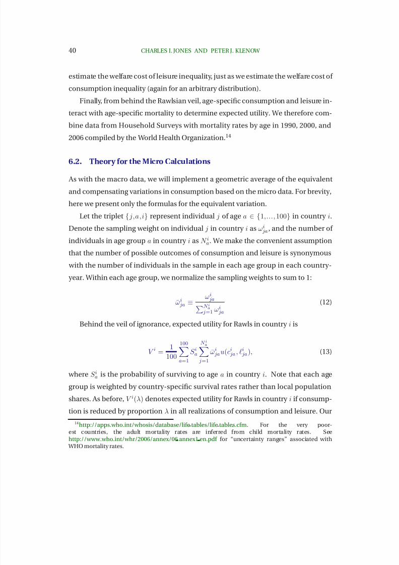
8/2/2019 Beyond GDP Welfare
http://slidepdf.com/reader/full/beyond-gdp-welfare 41/55
40 CHARLES I. JONES AND PETER J. KLENOW
estimate the welfare cost of leisure inequality, just as we estimate the welfare cost of
consumption inequality (again for an arbitrary distribution).
Finally, from behind the Rawlsian veil, age-specific consumption and leisure in-
teract with age-specific mortality to determine expected utility. We therefore com-
bine data from Household Surveys with mortality rates by age in 1990, 2000, and
2006 compiled by the World Health Organization.14
6.2. Theory for the Micro Calculations
As with the macro data, we will implement a geometric average of the equivalent
and compensating variations in consumption based on the micro data. For brevity,
here we present only the formulas for the equivalent variation.
Let the triplet { j,a,i} represent individual j of age a ∈ {1,..., 100} in country i.
Denote the sampling weight on individual j in country i as ωi ja , and the number of
individuals in age group a in country i as N ia. We make the convenient assumption
that the number of possible outcomes of consumption and leisure is synonymous
with the number of individuals in the sample in each age group in each country-
year. Within each age group, we normalize the sampling weights to sum to 1:
ωi ja ≡ ωi jaN ia
j=1 ωi ja
(12)
Behind the veil of ignorance, expected utility for Rawls in country i is
V i =1
100
100a=1
S ia
N ia j=1
ωi jau(ci ja , ℓi ja), (13)
where S ia is the probability of surviving to age a in country i. Note that each age
group is weighted by country-specific survival rates rather than local population
shares. As before, V i(λ) denotes expected utility for Rawls in country i if consump-
tion is reduced by proportion λ in all realizations of consumption and leisure. Our
14http://apps.who.int/whosis/database/life tables/life tables.cfm.. For the very poor-est countries, the adult mortality rates are inferred from child mortality rates. Seehttp://www.who.int/whr/2006/annex/06 annex1 en.pdf for “uncertainty ranges” associated with WHO mortality rates.
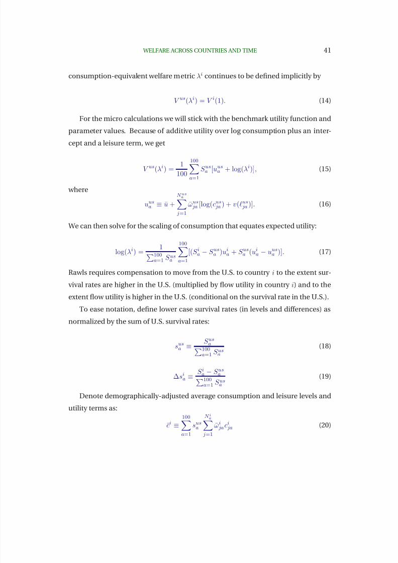
8/2/2019 Beyond GDP Welfare
http://slidepdf.com/reader/full/beyond-gdp-welfare 42/55
WELFARE ACROSS COUNTRIES AND TIME 41
consumption-equivalent welfare metric λi continues to be defined implicitly by
V us(λi) = V i(1). (14)
For the micro calculations we will stick with the benchmark utility function and
parameter values. Because of additive utility over log consumption plus an inter-
cept and a leisure term, we get
V us(λi) =1
100
100a=1
S usa [uusa + log(λi)], (15)
where
uusa ≡ u +
N us
a j=1
ωus ja [log(cus ja ) + v(ℓus ja )]. (16)
We can then solve for the scaling of consumption that equates expected utility:
log(λi) =1
100
a=1 S usa
100a=1
[(S ia − S usa )uia + S usa (ui
a − uusa )]. (17)
Rawls requires compensation to move from the U.S. to country i to the extent sur-
vival rates are higher in the U.S. (multiplied by flow utility in country i) and to the
extent flow utility is higher in the U.S. (conditional on the survival rate in the U.S.).
To ease notation, define lower case survival rates (in levels and differences) as
normalized by the sum of U.S. survival rates:
susa ≡ S usa100
a=1 S usa(18)
∆sia ≡ S ia − S usa
100
a=1 S usa(19)
Denote demographically-adjusted average consumption and leisure levels and
utility terms as:
ci ≡100a=1
susa
N ia j=1
ωi jaci ja (20)
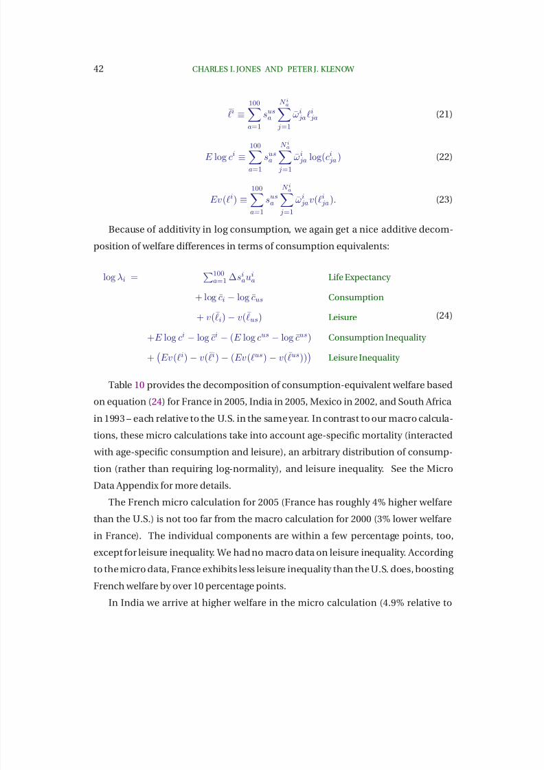
8/2/2019 Beyond GDP Welfare
http://slidepdf.com/reader/full/beyond-gdp-welfare 43/55
42 CHARLES I. JONES AND PETER J. KLENOW
ℓi ≡100a=1
susa
N ia j=1
ωi jaℓi ja (21)
E log ci ≡100a=1
susa
N ia j=1
ωi ja log(ci ja) (22)
Ev(ℓi) ≡100a=1
susa
N ia j=1
ωi jav(ℓi ja). (23)
Because of additivity in log consumption, we again get a nice additive decom-
position of welfare differences in terms of consumption equivalents:
log λi =
100
a=1 ∆siauia Life Expectancy
+ log ci − log cus Consumption
+ v(ℓi) − v(ℓus) Leisure
+E log ci − log ci − (E log cus − log cus) Consumption Inequality
+
Ev(ℓi) − v(ℓi) − (Ev(ℓus) − v(ℓus))
Leisure Inequality
(24)
Table 10 provides the decomposition of consumption-equivalent welfare based
on equation (24) for France in 2005, India in 2005, Mexico in 2002, and South Africain 1993 – each relative to the U.S. in the same year. In contrast to our macro calcula-
tions, these micro calculations take into account age-specific mortality (interacted
with age-specific consumption and leisure), an arbitrary distribution of consump-
tion (rather than requiring log-normality), and leisure inequality. See the Micro
Data Appendix for more details.
The French micro calculation for 2005 (France has roughly 4% higher welfare
than the U.S.) is not too far from the macro calculation for 2000 (3% lower welfare
in France). The individual components are within a few percentage points, too,except for leisure inequality. We had no macro data on leisure inequality. According
to the micro data, France exhibits less leisure inequality than the U.S. does, boosting
French welfare by over 10 percentage points.
In India we arrive at higher welfare in the micro calculation (4.9% relative to
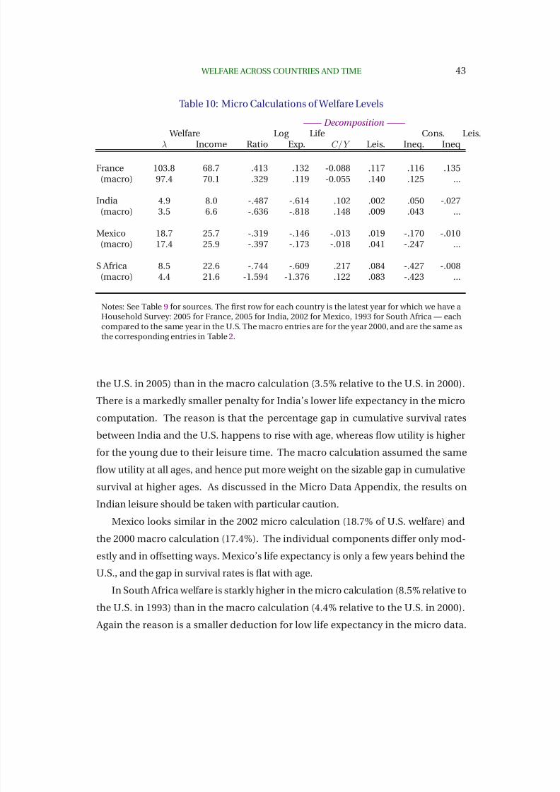
8/2/2019 Beyond GDP Welfare
http://slidepdf.com/reader/full/beyond-gdp-welfare 44/55
WELFARE ACROSS COUNTRIES AND TIME 43
Table 10: Micro Calculations of Welfare Levels
—— Decomposition —— Welfare Log Life Cons. Leis.
λ Income Ratio Exp. C/Y Leis. Ineq. Ineq
France 103.8 68.7 .413 .132 -0.088 .117 .116 .135(macro) 97.4 70.1 .329 .119 -0.055 .140 .125 ...
India 4.9 8.0 -.487 -.614 .102 .002 .050 -.027(macro) 3.5 6.6 -.636 -.818 .148 .009 .043 ...
Mexico 18.7 25.7 -.319 -.146 -.013 .019 -.170 -.010(macro) 17.4 25.9 -.397 -.173 -.018 .041 -.247 ...
S Africa 8.5 22.6 -.744 -.609 .217 .084 -.427 -.008
(macro) 4.4 21.6 -1.594 -1.376 .122 .083 -.423 ...
Notes: See Table 9 for sources. The first row for each country is the latest year for which we have aHousehold Survey: 2005 for France, 2005 for India, 2002 for Mexico, 1993 for South Africa — eachcompared to the same year in the U.S. The macro entries are for the year 2000, and are the same asthe corresponding entries in Table 2.
the U.S. in 2005) than in the macro calculation (3.5% relative to the U.S. in 2000).
There is a markedly smaller penalty for India’s lower life expectancy in the micro
computation. The reason is that the percentage gap in cumulative survival rates
between India and the U.S. happens to rise with age, whereas flow utility is higher
for the young due to their leisure time. The macro calculation assumed the same
flow utility at all ages, and hence put more weight on the sizable gap in cumulative
survival at higher ages. As discussed in the Micro Data Appendix, the results on
Indian leisure should be taken with particular caution.
Mexico looks similar in the 2002 micro calculation (18.7% of U.S. welfare) and
the 2000 macro calculation (17.4%). The individual components differ only mod-
estly and in offsetting ways. Mexico’s life expectancy is only a few years behind the
U.S., and the gap in survival rates is flat with age.
In South Africa welfare is starkly higher in the micro calculation (8.5% relative to
the U.S. in 1993) than in the macro calculation (4.4% relative to the U.S. in 2000).
Again the reason is a smaller deduction for low life expectancy in the micro data.
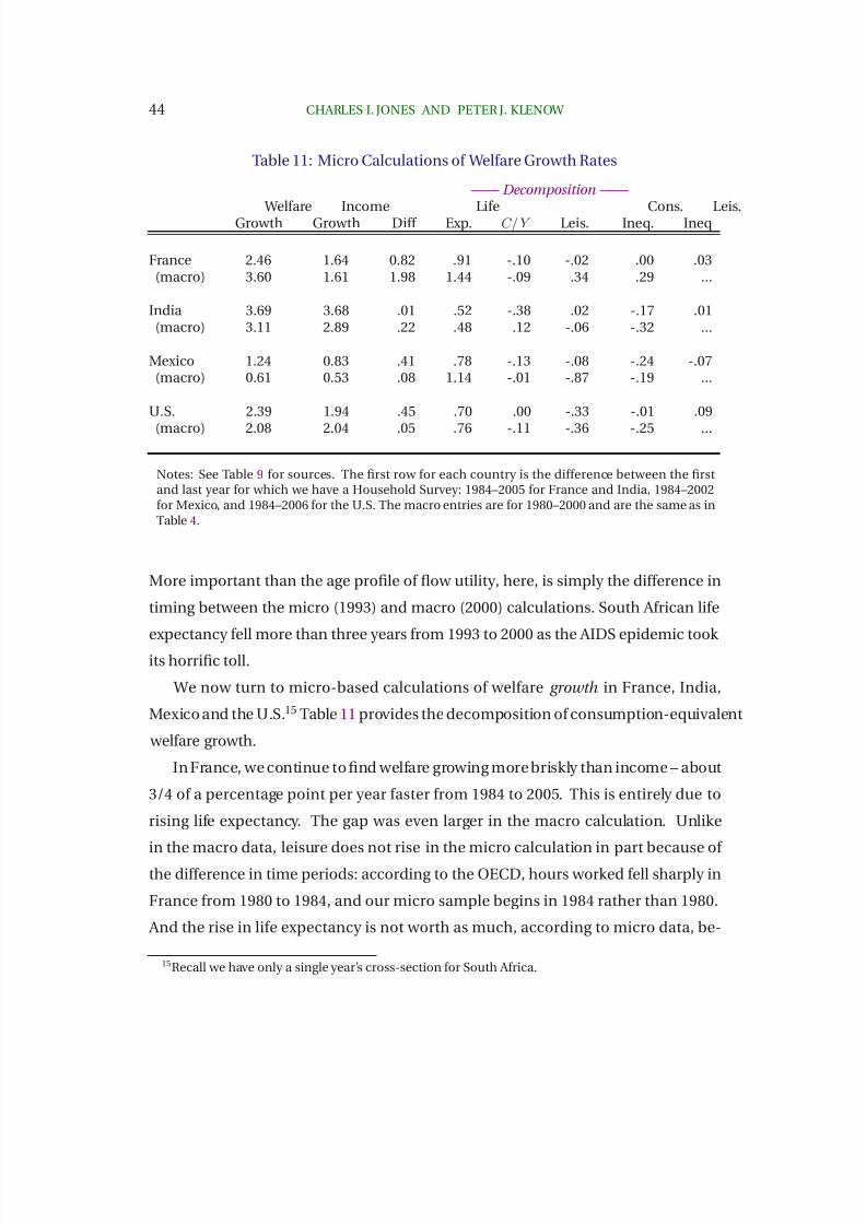
8/2/2019 Beyond GDP Welfare
http://slidepdf.com/reader/full/beyond-gdp-welfare 45/55
44 CHARLES I. JONES AND PETER J. KLENOW
Table 11: Micro Calculations of Welfare Growth Rates
—— Decomposition —— Welfare Income Life Cons. Leis.Growth Growth Diff Exp. C/ Y Leis. Ineq. Ineq
France 2.46 1.64 0.82 .91 -.10 -.02 .00 .03(macro) 3.60 1.61 1.98 1.44 -.09 .34 .29 ...
India 3.69 3.68 .01 .52 -.38 .02 -.17 .01(macro) 3.11 2.89 .22 .48 .12 -.06 -.32 ...
Mexico 1.24 0.83 .41 .78 -.13 -.08 -.24 -.07(macro) 0.61 0.53 .08 1.14 -.01 -.87 -.19 ...
U.S. 2.39 1.94 .45 .70 .00 -.33 -.01 .09
(macro) 2.08 2.04 .05 .76 -.11 -.36 -.25 ...
Notes: See Table 9 for sources. The first row for each country is the difference between the firstand last year for which we have a Household Survey: 1984–2005 for France and India, 1984–2002for Mexico, and 1984–2006 for the U.S. The macro entries are for 1980–2000 and are the same as inTable 4.
More important than the age profile of flow utility, here, is simply the difference in
timing between the micro (1993) and macro (2000) calculations. South African life
expectancy fell more than three years from 1993 to 2000 as the AIDS epidemic took
its horrific toll.
We now turn to micro-based calculations of welfare growth in France, India,
Mexico and the U.S.15 Table 11 provides the decomposition of consumption-equivalent
welfare growth.
In France, we continue to find welfare growing more briskly than income – about
3/4 of a percentage point per year faster from 1984 to 2005. This is entirely due to
rising life expectancy. The gap was even larger in the macro calculation. Unlike
in the macro data, leisure does not rise in the micro calculation in part because of
the difference in time periods: according to the OECD, hours worked fell sharply in
France from 1980 to 1984, and our micro sample begins in 1984 rather than 1980.
And the rise in life expectancy is not worth as much, according to micro data, be-
15Recall we have only a single year’s cross-section for South Africa.
8/2/2019 Beyond GDP Welfare
http://slidepdf.com/reader/full/beyond-gdp-welfare 46/55
WELFARE ACROSS COUNTRIES AND TIME 45
cause it occurred more for the middle-aged (with low leisure) rather than the young
(with high leisure).
In India, we find that welfare grew similarly to income (at 3.7% per year from
1983–2005). In our macro calculation, welfare actually grew 20 basis points faster
than income — mostly because C/Y actually rose from 1980–2000, whereas it fell
from 1983–2005.
In Mexico, household surveys suggest welfare rose a little more quickly than in-
come per year from 1984 to 2002 (1.2% annual growth in welfare vs. 0.8% annual
growth in incomes). The primary reason was rising life expectancy. The same state-
ments are true of the macro results, although the macro calculations featured bigger
gains from longer lives offset by falling leisure.
In the U.S., the Consumer Expenditure Survey yields an estimate of welfare growth
that is 45 basis points faster than income growth from 1984–2006. Gains from rising
life expectancy were offset by falling average time devoted to leisure.16 The CES
evinces no rise in consumption inequality, as emphasized by Krueger and Perri
(2006). In contrast, our macro calculation inferred rising consumption inequality
from rising income inequality, so that welfare and income growth were quite similar
from 1980–2000. According to Aguiar and Bils (2009), savings and Engel Curves in
the CES suggest that consumption inequality did rise as much as income inequality
in the U.S. over this period.
On the issue of consumption inequality, with the micro data an additional ro-
bustness check is possible. Recall that our measure of average consumption in-
cludes government consumption per capita (e.g., on public education and health
care). Yet both the macro Gini coefficients and the preceding micro calculations
were based on inequality in private consumption alone. This is tantamount to as-
suming that private consumption is proportional to total consumption. A polar as-
sumption would be that there is no variation in government consumption across
individuals. We therefore recalculate all of the consumption inequality terms in Ta-
ble 10 and Table 11 after adding equal per capita government consumption to all
16For the U.S. we also calculate a modest boost from falling leisure inequality. Using Time UseSurveys over a longer span, Aguiar and Hurst (2007) report rising leisure inequality in the U.S.
8/2/2019 Beyond GDP Welfare
http://slidepdf.com/reader/full/beyond-gdp-welfare 47/55
46 CHARLES I. JONES AND PETER J. KLENOW
individuals within a given country-year. This naturally lowers the costs of inequal-
ity, especially in South Africa but also in India (where it falls by roughly half).
To summarize, the exact welfare numbers are clearly sensitive to using House-
hold Surveys directly to measure consumption inequality, average leisure, leisure
inequality, and the benefits of longer lives. But, reassuringly, none of the key points
we took away from the macro calculations is reversed in these micro calculations.
In terms of levels, France is much closer to the U.S. in welfare than income. In
contrast, each of the following widens the welfare vs. income gaps with the U.S.:
lower life expectancy in India, higher inequality in Mexico, and both shorter lives
and greater consumption inequality in South Africa. Rising life expectancy carries
welfare growth above income growth in France, Mexico and the U.S. alike.
7. Caveats
Before concluding, we briefly discuss some of the serious limitations to our welfare
measure.
Our flow welfare index does not get at discounted lifetime utility. To the extent
consumption, leisure, or life expectancy exhibit transition dynamics or even trend
breaks (as with China after 1978), lifetime utility could differ markedly from our
snapshot. This is all the more true if individual utility is not separable over time
so that mobility in consumption and leisure matter. If an individual or even whole
economy is transitioning to a higher level of consumption, current levels of con-
sumption can be too pessimistic about lifetime utility. We did note, however, that
most observed cross-country differences in consumption-output ratios reflect per-
sistent (steady state) differences rather than transition dynamics.
In a recursive world, one could take a value function approach, identifying the
state variables that matter for discounted welfare. Relevant states might include the
stocks of human and physical capital, TFP in producing final goods and health, and
the degree of consumption insurance.17 An advantage of this complementary value
17Related, Basu, Pascali, Schiantarelli and Serven (2010) suggest that totalfactor productivity growthmay, under quite general circumstances, be interpreted as a measure of welfare growth.
8/2/2019 Beyond GDP Welfare
http://slidepdf.com/reader/full/beyond-gdp-welfare 48/55
WELFARE ACROSS COUNTRIES AND TIME 47
function approach is that it might shed light on underlying policy distortions, as
opposed to simply evaluating outcomes.
We evaluate outcomes in terms of a single utility function both within and across
countries. In contrast, preference heterogeneity (at least within countries) is a rou-
tine assumption in labor economics and public finance. See Weinzierl (2009) for
a recent discussion of how preference heterogeneity can affect optimal taxation.
Although we believe it is beyond the scope of this paper, one could try to use house-
hold data to quantify preference heterogeneity within countries.
A related issue is whether countries differ in the efficiency of time spent in home
production. For example, human capital is surely useful at home (e.g. in childcare)
as well as in the market. To the extent the benefits take the form of future con-
sumption, our flow welfare index could pick this up eventually. Also, if leisure is
more productive because of a higher quality and quantity of consumer durables,
then this could arguably be dealt with by nonseparable momentary utility between
consumption and leisure.
Our narrow utility over consumption and leisure ignores altruism, for example
within families. Given the big differences in family size and population growth rates
across countries (e.g., Tertilt (2005)), incorporating intergenerational altruism could
have a first order effect on welfare calculations.
Our measure of health focuses on the easier-to-measure extensive margin (quan-
tity of life), following a long tradition; see especially Nordhaus (2003). However, the
intensive margin (quality of life) is obviously important as well. To the extent we in-
clude health spending in our measure of consumption, one could argue we are cap-
turing the intensive margin across countries, and maybe even double-counting the
extensive margin. But this ignores differences in the natural disease environment
that may cause differences in morbidity for a given amount of health spending (e.g.
the prevalence of malaria). Moreover, in the cross-section within countries, health
may be negatively correlated with health spending (e.g. across age groups).18
18 A large recent literature also emphasizes the possible causal links between health and growth: forexample Acemoglu and Johnson (2007), Bleakley (2007), Weil (2007), Feyrer, Politi and Weil (2008),and Aghion, Howitt and Murtin (2010).
8/2/2019 Beyond GDP Welfare
http://slidepdf.com/reader/full/beyond-gdp-welfare 49/55
48 CHARLES I. JONES AND PETER J. KLENOW
Some of our parameter values implied negative average flow utility in the very
poorest countries. This understates welfare in these countries, to put it mildly. With
estimates of the value of life in some of the poorest countries, one could get a sense
for how badly this misses the mark.19 One could also incorporate heterogeneity in
mortality rates within a country; Edwards (2010) suggests that this may be quantita-
tively significant in his extension of the Becker, Philipson and Soares (2005) growth
rates.
We have neglected the natural environment more generally. The quality of the
air, water, and so on provide utility for a given amount of market consumption and
leisure and help sustain future consumption. See, for example, U.S. Bureau of Eco-
nomic Analysis (1994), Dasgupta (2001) and Arrow et al. (2004).
There have been various efforts to quantify the economic costs of crime (in-
cluding prevention), such as Anderson (1999). Possibly related, Nordhaus and To-
bin (1972) subtracted urban disamenities in calculating their Measure of Economic
Welfare.
The data we use for aggregate real consumption per capita is converted into dol-
lars using estimated PPP exchange rates. The underlying price ratios are supposed
to be for comparable-quality goods and services. But in practice it can be diffi-
cult to fully control for quality differences, especially for education and health. And
the current methodology makes no attempt to quantify differences in variety across
countries. Any errors in the PPP exchange rate for consumption will contaminate
the consumption portion of our welfare index.
Related, households in a given country may face different price indices (inclu-
sive of variety and quality). If so, then expenditures are not proportional to true
consumption within countries, as we have assumed. If true price indices are posi-
tively correlated with expenditures (i.e., prices are lower in poorer areas), then the
Gini coefficients we use overstate consumption inequality.
Finally, we have not experimented with non-standard preferences such as habit
formation or keeping up with the Joneses. Doing so could imply smaller differences
19In this vein, Kremer, Leino, Miguel and Zwane (2009) use valuation of clean water in rural Kenyato estimate the implied value of averting a child death at between $769 and $3006.

8/2/2019 Beyond GDP Welfare
http://slidepdf.com/reader/full/beyond-gdp-welfare 50/55
WELFARE ACROSS COUNTRIES AND TIME 49
in flow utility from gaps in average consumption across countries. How these alter-
native preferences would affect the welfare costs of inequality is less clear.
8. Conclusion
For a given specification of preferences, we calculate consumption-equivalent wel-
fare for various countries and years using widely available data on average con-
sumption, average leisure, consumption inequality, and average life expectancy.
Several findings stand out.
First, the correlation between our welfare index and income per capita is very
high. This is because average consumption differs so much across countries and
is strongly correlated with income. Second, living standards in Western Europe
are much closer to those in the United States than it would appear from GDP per
capita. Longer lives with more leisure time and more equal consumption in West-
ern Europe largely offset their lower average consumption vis a vis the United States.
Third, in most developing economies, welfare is markedly lower than income, due
primarily to shorter lives but also to more inequality. Finally, rising life expectancy
accounts for about 1/3 of welfare growth in the U.S. and Western Europe and all of
average welfare growth in Latin America (given declining welfare from other sources).
In contrast, life expectancy actually declines between 1980 and 2000 in many coun-
tries in sub-Saharan Africa, reducing welfare and expanding the development gap
between these countries and the rest of the world.
For a small set of countries (the U.S., France, India, Mexico, and South Africa),
we exploited household surveys on consumption and leisure. With such micro data
we can incorporate all of the above, plus leisure inequality and age-specific mortal-
ity. These “micro” results are broadly similar to our findings with “macro” data.
Our calculations entail many strong assumptions. We therefore checked robust-
ness to alternative welfare measures and alternative utility functions over consump-
tion and leisure. Our benchmark calculations are quite representative of the differ-
ences between welfare and income we see in the robustness checks. For the limited
set of countries for which we analyzed micro data, we were able to drop several
8/2/2019 Beyond GDP Welfare
http://slidepdf.com/reader/full/beyond-gdp-welfare 51/55
50 CHARLES I. JONES AND PETER J. KLENOW
simplifying assumptions (e.g. log-normally distributed consumption).
With the requisite data, one could relax many more of our assumptions. Life
expectancy surely differs by more than age within countries (e.g. by education).
Preferences over consumption and leisure must differ within countries, perhaps
mitigating the welfare cost of unequal outcomes. Where household data is avail-
able going back far enough, one could try to estimate the present discounted value
of welfare.20
One could carry out similar calculations across geographic regions within coun-
tries, or for that matter across subgroups of a country’s population (e.g., by gender
or race). Even more ambitious, but conceivable, would be to try to account for some
of the many important factors we omitted entirely, such as morbidity, the quality of
the natural environment, crime, political freedoms, and intergenerational altruism.
We hope our simple measure proves to be a useful building block for work in this
area.
A Data Appendix
Extended results for all countries as well as the basic data used in our calculations
is available at http://www.stanford.edu/∼chadj/BasicDataRawls10.xls. A detailed
data appendix and descriptions of the programs used to compute the results are
available at http://www.stanford.edu/∼chadj/Rawls-DataAppendix200.pdf .
References
Acemoglu, Daron and Simon Johnson, “Disease and development: the Effect of Life Ex-
pectancy on Economic Growth,” Journal of Political Economy , 2007, 115 (6), 925–985.
Aghion, Philippe, Peter Howitt, and Fabrice Murtin, “The Relationship Between Health and
Growth: When Lucas Meets Nelson-Phelps,” NBER Working Paper 15813 March 2010.
20 With time-separable utility, repeated cross-sections would suffice. Dealing with nonseparability over time, however, would seem to require longer household panels than are known to us.
8/2/2019 Beyond GDP Welfare
http://slidepdf.com/reader/full/beyond-gdp-welfare 52/55
WELFARE ACROSS COUNTRIES AND TIME 51
Aguiar, Mark and Erik Hurst, “Measuring Trends in Leisure: The Allocation of Time over Five
Decades,” Quarterly Journal of Economics , 08 2007, 122 (3), 969–1006.
and Mark Bils, “Has Consumption Inequality Mirrored Income Inequality?,” December
2009. University of Rochester mimeo.
Aitchison, J. and J.A.C. Brown, The Lognormal Distribution with Special Reference to its Uses
in Economics , Cambridge University, London, 1957.
Anderson, David A., “The Aggregate Burden of Crime,” Journal of Law and Economics , Oc-
tober 1999, 42 , 611–642.
Arrow, Kenneth, Partha Dasgupta, Lawrence Goulder, Gretchen Daily, Paul Ehrlich, Geof-
frey Heal, Simon Levin, Karl-Goran Maler, Stephen Schneider, David Starrett, and Brian
Walker, “Are We Consuming Too Much?,” Journal of Economic Perspectives , Summer 2004,
18 (3), 147–172.
Ashenfelter, Orley and Michael Greenstone, “Using Mandated Speed Limits to Measure the
Value of a Statistical Life,” Journal of Political Economy , February 2004, 112 (1), S226–
S267. Part 2.
Barro, Robert J. and Charles J. Redlick, “Macroeconomic Effects from Government Pur-
chases and Taxes,” NBER Working Paper 15369 September 2009.
Basu, Susanto, Luigi Pascali, Fabio Schiantarelli, and Luis Serven, “Productivity, Welfare andReallocation: Theory and Firm Level Evidence,” Boston College manuscript June 2010.
Battistin, Erich, Richard Blundell, and Arthur Lewbel, “Why is Consumption More Log Nor-
mal Than Income? Gibrat’s Law Revisited,” Journal of Political Economy , December 2009,
117 (6), 1140–1154.
Becker, Gary S., Tomas J. Philipson, and Rodrigo R. Soares, “The Quantity and Quality of Life
and the Evolution of World Inequality,” American Economic Review , March 2005, 95 (1),
277–291.
Bleakley, Hoyt, “Disease and Development: Evidence from Hookworm Eradication in the
American South,” The Quarterly Journal of Economics , February 2007, 122 (1), 73–117.
Boarini, Romina, Asa Johansson, and Marco Mira d’Ercole, “Alternative Measures of Well-
Being,” OECD Social, Employment and Migration Working Papers 33, OECD, Directorate
for Employment, Labour and Social Affairs February 2006.
8/2/2019 Beyond GDP Welfare
http://slidepdf.com/reader/full/beyond-gdp-welfare 53/55
52 CHARLES I. JONES AND PETER J. KLENOW
Chetty, Raj, “Bounds on Elasticities with Optimization Frictions: A Synthesis of Micro and
Macro Evidence on Labor Supply,” NBER Working Paper 15616 December 2009.
Dasgupta, Partha, Human Well-Being and the Natural Environment , Oxford and New York:
Oxford University Press, 2001.
Edwards, Ryan D., “The Cost of UncertainLife Span,” Queen’s College manuscript May 2010.
Feyrer, James., Dimitra Politi, and David N. Weil, “The Economic Effects of Micronutrient
Deficiency: Evidence from Salt Iodization in the United States,” manuscript, Brown Uni-
versity , 2008.
Fleurbaey, Marc, “Beyond GDP: The Quest for a Measure of Social Welfare,” Journal of Eco-
nomic Literature , December 2009,
47 (4), 1029–1075.
and Guillaume Gaulier, “International Comparisons of Living Standards by Equivalent
Incomes,” Scandinavian Journal of Economics , 09 2009, 111 (3), 597–624.
Hall, Robert E., “By How Much Does GDP Rise If the Government Buys More Output?,”
Brookings Papers on Economic Activity , September 2009, 11.
, “Reconciling Cyclical Movements in the Marginal Value of Time and the Marginal Prod-
uct of Labor,” Journal of Political Economy , 2009, 117 (2), 281–323.
Heathcote, Jonathan, Kjetil Storesletten, and Giovanni L. Violante, “Insurance and Oppor-
tunities: A Welfare Analysis of Labor Market Risk,” Journal of Monetary Economics , April
2008, 55 (3), 501–525.
Kremer, Michael, Jessica Leino, Edward Miguel, and Alix Peterson Zwane, “Spring Cleaning:
Rural Water Impacts, Valuation and Property Rights Institutions,” August 2009. NBER
Working Paper No. 15280.
Krueger, Dirk and Fabrizio Perri, “Does Income Inequality Lead to Consumption Inequality?
Evidence and Theory,” Review of Economic Studies , January 2006, 73 (1), 163–193.
, , Luigi Pistaferri, and Giovanni L. Violante, “Cross Sectional Facts for Macroe-conomists,” Review of Economic Dynamics , January 2010, 13 (1), 1–14.
Lucas, Robert E., Models of Business Cycles , New York: Basil Blackwell, 1987.
Murphy, Kevin M. and Robert H. Topel, “The Value of Health and Longevity,” Journal of
Political Economy , October 2006, 114 (5), 871–904.
8/2/2019 Beyond GDP Welfare
http://slidepdf.com/reader/full/beyond-gdp-welfare 54/55
WELFARE ACROSS COUNTRIES AND TIME 53
Nordhaus, William D., “The Health of Nations: The Contribution of Improved Health to
Living Standards,” in Kevin M. Murphy and Robert Topel, eds., Measuring the Gains from
Medical Research: An Economic Approach , Chicago: University of Chicago Press, 2003,pp. 9–40.
and James Tobin, “Is Growth Obsolete?,” in “Economic Research: Retrospect and
Prospect Vol 5: Economic Growth,” National Bureau of Economic Research, Inc, Decem-
ber 1972, pp. 1–80.
Ohanian, Lee, Andrea Raffo, and Richard Rogerson, “Long-Term Changes in Labor Supply
and Taxes: Evidence from OECD Countries, 1956-2004,” Journal of Monetary Economics ,
November 2008, 55 , 1353–1362.
Parente, Stephen L., Richard Rogerson, and Randall Wright, “Homework in Development
Economics: Household Production and the Wealth of Nations,” Journal of Political Econ-
omy , August 2000, 108 (4), 680–687.
Pistaferri, Luigi, “Anticipated and Unanticipated Wage Changes, Wage Risk, and Intertem-
poral Labor Supply,” Journal of Labor Economics , 2003, 21 (3), 729–754.
Prescott, Edward C., “Why Do Americans Work So Much More than Europeans?,” Quarterly
Review , July 2004, pp. 2–13.
Rawls, John, A Theory of Justice , Harvard University Press, 1971.
Shimer, Robert, “Convergence in Macroeconomics: The Labor Wedge,” American Economic
Journal: Macroeconomics , January 2009, 1 (1), 280–297.
Stiglitz, Joseph E., Amartya Sen, and Jean-Paul Fitoussi, “Report by the Commission on the
Measurement of Economic Performance and Social Progress,” Technical Report Septem-
ber 2009.
Tertilt, Michele, “Polygyny, Fertility, and Savings,” Journal of Political Economy , 12 2005, 113
(6), 1341–1371.
Trabandt, Mathias and Harald Uhlig, “How Far Are We From The Slippery Slope? The Laffer
Curve Revisited,” NBER Working Paper 15343 September 2009.
U.S. Bureau of Economic Analysis, “Integrated Economic and Environmental Satellite Ac-
counts,” Survey of Current Business , April 1994, 74 , 33–49.
8/2/2019 Beyond GDP Welfare
http://slidepdf.com/reader/full/beyond-gdp-welfare 55/55