Embed Size (px)
Citation preview

RIGHT:
URL:
CITATION:
AUTHOR(S):
ISSUE DATE:
TITLE:
Bias-Adjustment of Satellite-Based RainfallEstimates over the Central Himalayas ofNepal for Flood Prediction( Dissertation_全文 )
SHRESTHA, Mandira Singh
SHRESTHA, Mandira Singh. Bias-Adjustment of Satellite-Based Rainfall Estimates over the Central Himalayas of Nepalfor Flood Prediction. 京都大学, 2011, 博士(工学)
2011-03-23
https://doi.org/10.14989/doctor.r12546

Bias-Adjustment of Satellite-Based Rainfall Estimates
over the Central Himalayas of Nepal for Flood
Prediction
By
Mandira Singh SHRESTHA
2011


Bias-Adjustment of Satellite-Based Rainfall Estimates
over the Central Himalayas of Nepal for Flood
Prediction
By
Mandira Singh SHRESTHA
A Dissertation
Submitted in partial fulfillment of the requirement for the
Degree of Doctor of Engineering
Department of Civil and Earth Resources Engineering
Kyoto University, Japan
2011


PhD Dissertation
i
Acknowledgements
I would like to first and foremost express my heartfelt gratitude to my principal supervisor Prof
Kaoru Takara. His guidance, support and continuous encouragement have enabled me to
complete my research. He has shown great patience, kindness and provided excellent motivation
throughout the course of my doctoral degree. Without his understanding and guidance the
completion of my doctoral degree would have remained a farfetched dream.
I would also like to express my gratitude to Prof Yosuke Yamashiki who has provided
support and guidance during my doctoral study. My gratitude also goes to Dr Kobayashi
Kenichiro who I have consulted with during the preparation of this thesis as well as Prof Eiichi
Nakakita, Prof Takashi Hosoda and Prof Yasuto Tachikawa for their reviewing the thesis and
qualifying my PhD. I would also like to thank Ms Sono Innou and Ms Yuko Takii for their
administrative support and Mr Fuiki Shigeo and Mr Tsuato Oizumi for their technical support
while I was in Japan.
My gratitude also goes to Japan Society for the Promotion of Science (JSPS) for providing
me the RONPAKU scholarship without which I would not have been able to complete this
doctoral dissertation. I am grateful for the flexibility and the opportunity provided by such a
program that enables people engaged in research like me to carry out a doctoral degree. It is
indeed a very good opportunity and must thank the Government of Japan for providing such a
scholarship.
I would like to thank Dr Andreas Schild, Director General of the International Centre for
Integrated Mountain Development (ICIMOD) for his continuous support and encouragement in
enabling me to complete my PhD degree. His understanding and support towards staff’s
wellbeing and professional development is much appreciated. Without this understanding and
support I would not have been able to participate in such a doctoral dissertation program. Prof
Hua Ouyang, Programme Manager of the Integrated Water and Hazard Management (IWHM)
program of ICIMOD is another person I would like to thank. He kept encouraging me and
motivating me to complete this dissertation on time despite a number of activities that had to
remain on hold. I would also like to thank Dr Arun Bhakta Shrestha, and Mr Pradeep Mool,
Teamleaders for their patience, understanding and encouragement and all my colleagues at
IWHM. I would also like to thank my colleague Dr Beatrice Murray who is a good friend and

PhD Dissertation
ii
colleague and provided the much needed advice and encouragement during hard times. My
appreciation and deep sense of gratitude is also for Prof Suresh Raj Chalise who are amongst
those that inspired me to pursue a doctoral degree.
This doctoral research is part of a project “Application of Satellite Rainfall Estimation in the
Hindu-Kush Himalayan region” funded by USAID/OFDA under the Asia Flood Network
Program. I would like to take this opportunity to express my gratitude to United States Agency
for International Development Office of US Foreign Disaster Assistance (USAID/OFDA) for the
funding and Dr Sezin Tokar, hydrometeorological advisor of USAID/OFDA for her continuous
support and encouragement. Her guidance, encouragement and kind words have provided me the
energy and motivation to complete my thesis. I would like to thank Dr Guleid Artan from USGS
who is my mentor and “Guru” particularly on the hydrological modelling and analysis part. His
patience in answering my simple and at times difficult questions through long distance
communication was very helpful. I would also like to thank Dr Tim Love and Mr Eric
Wolvovsky from National Oceanic and Atmospheric Administration (NOAA) for familiarizing
me with the NOAA CPC_RFE2.0 satellite-based rainfall product. The kind advise and support of
Dr Takuji Kubota from Japan Aerospace Exploration Agency (JAXA) is also much appreciated.
I would like to thank my colleague Mr. Sagar Ratna Bajracharya who has been with me through
this whole research period and has worked very closely with me in different aspects of this
research. His pleasant attitude and willingness to help at all times of need has provided me the
support to learn from him some of the tedious ArcGIS modules much needed for the analysis. I
would also like to thank Mr. Rupak Rajbhandari for all the professional support and
contributions he has made to the project as well as all the regional partners from the Hindu Kush-
Himalayan region.
I would like to thank the Department of Hydrology and Meteorology (DHM) for providing
the data for the research and to Dr Dilip Gautam and Mr Rishi Ram Sharma from DHM in
particular, for their constructive engagement in the project.
Last but not the least there are a whole group of people close to my heart I would like to
thank. My mother Mrs Indira Shrestha has been my principal motivator. “Yes you can do it” is
what she told me at all stages of this doctoral dissertation – “without pain there is no gain” is
what she reminded me of every time I felt a little distracted. My mother in law Mrs Yanchu
Singh always provided me that feeling of security and confidence. While I was away for the
doctoral study she took care of the family despite her occasional ill health and gave me that

PhD Dissertation
iii
freedom to do what I always wanted to do. My sister Bandana Shrestha and brother Jay Pal
Shrestha have pushed me towards completing my dissertation with encouraging words at all
times. My children Juni, Manzari and Ravi have also been very supportive and understanding.
“Go do it Mamu – we will take care of ourselves while you are away” was what they use to tell
me providing me that much needed support and understanding despite their mother being away.
Finally, my gratitude goes to my beloved husband Mr. B.K. Man Singh who has been the man
holding the candle for me in the darkness at all times. His love, sincerity and constant
encouragement has made me complete this dissertation.
Thank you all very much.
Mandira Singh Shrestha

PhD Dissertation
iv

PhD Dissertation
v
Abstract
This research is a part of a long term regional project on “Application of Satellite Rainfall
Estimation in the Hindu Kush-Himalayan Region” implemented by the International Centre for
Integrated Mountain Development (ICIMOD) and the regional partners.
Flood disasters are recurrent in Nepal leading to huge loss of lives, infrastructure damage and
adverse impacts on socioeconomic development. An important approach to non-structural flood
management lies in the provision of an end-to-end flood forecasting and warning services. Due
to the limited spatial coverage of ground based gauges, unavailability of real-time rainfall data,
and constraint in technical and financial resources, the Department of Hydrology and
Meteorology (DHM) of Nepal is yet to initiate an operational flood forecasting. The availability
of global coverage of satellite data offer effective and economical means of calculating areal
rainfall estimates in sparsely gauged areas. Thus, satellite-based rainfall estimates (SRE) may be
one of the best and appropriate approaches for Nepal to predict and forecast rainfall-induced
runoff that may produce flooding.
Satellite-based rainfall estimation technology has rapidly developed in the last few decades
but this technology is still in its infancy in most of the Hindu Kush Himalayan (HKH) countries
including Nepal. A clear understanding of the satellite rainfall estimation methods and products
are a prerequisite to apply SRE for flood prediction. The research focussed on three broad
objectives (i) to evaluate the accuracy of SRE over the central himalayas of Nepal (ii) to improve
the SRE with bias-adjustment (iii) to improve the flood prediction by applying bias-adjustment.
This research carried out review of the various satellite-based rainfall estimation methods and
products. Quantitative validation of the National Oceanic and Atmospheric Administration
(NOAA) CPC-RFE2.0 (RFE) and Japan Aerospace Exploration Agency (JAXA)
GSMaP_MVK+ (GSMaP) products based on independent ground station observed data were
carried out. The verifications were conducted at three levels. The first set of verification was
conducted considering the whole country as one homogeneous region. The second level
verification was conducted partitioning the county into various physiographic regions and the
third was at river basin level. At a regional level the analysis data from 422 rainfall stations were
available for the verification out of which 176 are within Nepal for the period 2002 to 2006. The
accuracy of the SRE was evaluated using the standard verification technique which included
visual analysis as well as continuous verification statistics and categorical verification statistics.

PhD Dissertation
vi
Visual verification was subjective and compared maps of satellite estimates with observations.
The continuous verification statistics included correlation coefficient, root mean square error
(RMSE), bias, and percentage error, to provide a quantitative assessment for each set of
verification data. The categorical verification statistics were qualitative and included probability
of detection (i.e., events diagnosed correctly) and false-alarm ratio (which detects non-events).
The results in general show underestimation of rainfall in intense rainfall periods and heavy
rainfall regions and overestimation of rainfall in rainshadow and arid areas with both the SRE
products. In general the rainfall events matched qualitatively when spotting extreme rainfall, but
quantitatively there were some differences. The GSMaP estimates were found to underestimate
the whole Nepal averaged annual rainfall by 48 % and RFE by 30%. The daily bias averaged
over whole of Nepal was -1.1 mm/day with RFE and -2.0 mm/day with GSMaP for the period
2003 to 2006. The RMSE over whole of Nepal was -4.0 mm/day with RFE and -4.9 mm/day
with GSMaP for the same period. The bias and the RMSE were higher for the June July, August
and September (JJAS) period compared to the annual. The GSMaP however showed better
correlation with the observed data as compared to RFE.
The second level of verification was conducted for various physiographic regions to assess
the performance of RFE and GSMaP. Both SREs performed better in the flatter regions in the
Terai and Siwalik regions. The performance deteriorated with higher elevations with the
minimum performance in the High Mountains. The Middle Mountain regions despite denser
network of stations compared to other regions showed poorer performance of SREs. At the basin
level the bias was smaller in the Bagmati than the Narayani. These results indicate that overall
the SREs provides reasonable rainfall estimates but needs to be improved before it can be
implemented for operational flood forecasting.
The United States Geological Survey (USGS) GeoSpatial Streamflow Model (GeoSFM)
model was applied in two basins, the Bagmati and Narayani. In both basins there was a good
correlation between the simulated and observed discharge at Pandheradovan and Devghat using
gauge observed rainfall, for the period 2002-2004, with correlation values of 0.95 for Bagmati
and 0.94 for Narayani. With the RFE estimates the simulated discharges followed the trend of
the observed values quite well, although there was a significant difference in the magnitude of
the flows indicating a need for bias correction prior to application into operational flood
prediction.

PhD Dissertation
vii
With five years of data from 2002 to 2006; the seasonal, monthly and 7-day moving average
bias-adjustments were derived comparing the RFE rainfall estimates and gridded gauge observed
rainfall data at grids with one or more gauges. These bias-adjustments were applied to the RFE
to obtain a new set of rainfall estimates. These bias-adjusted rainfalls when applied to the
GeoSFM model resulted in improvement in flood prediction. The second approach of improving
the SREs was by ingesting additional local rain gauge data into the RFE algorithm (referred to as
“improved RFE”) by expanding the Global Telecommunication Satellite (GTS) data input. The
GeoSFM model calibrated with the gauge observation and the “improved RFE” provided
considerable improvement in flood prediction. However, there seemed to be some discrepancy in
the medium flow estimation. Therefore, keeping in mind the inherent errors in the SREs the
model was recalibrated with improved RFE. The recalibrated model with new gauge-satellite
merged rainfall estimates showed further improvement in the simulation of flows.
Overall, findings from this study indicate that the SRE underestimates rainfall significantly
over Nepal but with correlation higher than 0.70. The performance of the SRE is better in the
flatter terrain than in the mountainous areas. The accuracy of SREs can be improved by applying
a bias-adjustment. Prediction of discharge using bias-adjusted rainfall estimates can improve the
accuracy of discharge prediction with considerable increase in the predictive capability of flood
prediction for which the hydrological model needs to be recalibrated.

PhD Dissertation
viii

PhD Dissertation
ix
Acronym
AFN Asia Flood Network
AMSU Advanced Microwave Sounding Unit
AVHRR Advanced Very High Resolution Radiometer
CN Curve Number
CPC Climate Prediction Center
DEM Digital Elevation Model
DHM Department of Hydrology and Meteorology, Nepal
DMSP Defense Meteorological Satellite Program
DMSW Digital Soil Map of the World
EROS Earth Research Observation and Science
ESRI Environmental Systems Research Institute
FAO Food and Agricultural Organization
FAR False Alarm Ratio
FEWS Famine Early Warning System
GCM Global Climate Model
GDAS Global Data Assimilation System
GeoSFM Geospatial Streamflow Model
GIS Geographic Information System
GLCC Global Land Cover Characteristics
GLOF Glacial Lake Outburst Flood
GOES Geostationary Operational Environmental Satellite
GPCP Global Precipitation Climatology Project
GPI GOES Precipitation Index
GSMaP Global Satellite Mapping Project

PhD Dissertation
x
GTS Global Telecommunication System
GUI Graphical User Interface
HKH Hindu Kush-Himalayan
ICIMOD International Centre for Integrated Mountain Development
IDW Inverse Distance Weighted
INSAT Indian Satellite
IR Infra red
JAXA Japan Aerospace Exploration Agency
MAE Mean Absolute Error
MOSCEM Multiobjective Shuffled Complex Evolution Metropolis
MW Microwave
NOAA National Oceanic and Atmospheric Administration
NRL Naval Research Laboratory
OFDA Office of US Foreign Disaster Assistance
PET Potential Evapotranspiration
PERSIANN Precipitation Estimate from Remotely Sensed Information using Artificial Neural
Network
PMW Passive Microwave
POD Probability Of Detection
PR Precipitation Radar
RCM Regional Climate Model
RFE Rainfall Estimation
RMSE Root Mean Square Error
SA Sensitivity Analysis
SRE Satellite-based Rainfall Estimate
SSM/I Special Sensor Microwave / Imager

PhD Dissertation
xi
SWHC Soil Water Holding Capacity
TMI TRMM Microwave Imager
TMPA TRMM Multisensor Precipitation Analysis
TRMM Tropical Rainfall Measuring Mission
UNDP United Nations Development Programme
USAID The United States Agency for International Development
USGS United States Geological Survey
VIRS Visual Infra Red Scanner
VIS Visible
WMO World Meteorological Organization

PhD Dissertation
xii

PhD Dissertation
xiii
Table of Contents
Abstract ………………………………………………………………………………………….v
Acronyms ……………………………………………………………………………………….ix
List of Figures …………………………………………………………………………….…..xvii
List of Tables …………………………………………………………………………….….....xxi
1 INTRODUCTION ................................................................................................................. 1 1.1 Background ..................................................................................................................... 1
1.2 Identification of Problem ................................................................................................ 2
1.3 Background of the Research ........................................................................................... 5
1.4 Study Area ...................................................................................................................... 5
1.5 Objectives ....................................................................................................................... 7
1.6 Outline of the Thesis ....................................................................................................... 8
2 REVIEW OF GLOBAL SATELLITE-BASED RAINFALL ESTIMATION METHODS, PRODUCTS AND VERIFICATION ................................................................. 13
2.1 Satellite-Based Rainfall Estimation Methods ............................................................... 13
2.1.1 VIS/IR Method.......................................................................................................... 14
2.1.2 Passive Microwave method ...................................................................................... 15
2.1.3 Mutli-Sensor Technique............................................................................................ 16
2.2 Satellite Rainfall Estimate Products .............................................................................. 16
2.2.1 The NOAA CPC_RFE2.0 Satellite Rainfall Estimates ............................................ 16
2.2.2 The NOAA CMORPH Rainfall Estimates ............................................................... 19
2.2.3 Tropical Rainfall Measuring Mission (TRMM) ....................................................... 19
2.2.4 Global Satellite Mapping Project (GSMaP) ............................................................. 22
2.2.5 Precipitation Estimation from Remote Sensing Information using Artificial Neural
Network (PERSIANN) .......................................................................................................... 23
2.3 Review of Verification of Satellite-Based Rainfall Estimates ...................................... 25
2.4 Summary ....................................................................................................................... 31

PhD Dissertation
xiv
3 VERIFICATION OF SATELLITE-BASED RAINFALL ESTIMATES OVER CENTRAL HIMALAYAS OF NEPAL .................................................................................... 35
3.1 Methodology for Verification of Satellite-Based Rainfall Estimates ........................... 35
3.1.1 Visual Verification .................................................................................................... 36
3.1.2 Continuous Verification Technique .......................................................................... 36
3.1.3 Categorical Verification Technique .......................................................................... 38
3.2 Interpolation of the Observed Rainfall - Kriging .......................................................... 40
3.3 Verification of Satellite-Based Rainfall Estimates over Nepal ..................................... 42
3.3.1 Data Preparation ........................................................................................................ 43
3.3.2 Country Level Verification - Assessment of the Accuracy of the Satellite-Based
Rainfall Estimates over the Whole of Nepal ......................................................................... 45
3.3.3 Physiographic Level Verification - Assessment of the Accuracy of the Satellite-
Based Rainfall Estimates for Various Physiographic Regions .............................................. 60
3.3.4 Basin Level Verification in the Bagmati and Narayani Basins ................................ 65
3.4 Summary ....................................................................................................................... 75
4 RAINFALL-RUNOFF MODELLING USING SATELLITE-BASED RAINFALL ESTIMATES ............................................................................................................................... 79
4.1 Introduction ................................................................................................................... 79
4.2 The GeoSFM Model ..................................................................................................... 80
4.2.1 Introduction ............................................................................................................... 80
4.2.2 Model Formulation ................................................................................................... 82
4.3 Data Inputs .................................................................................................................... 83
4.3.1 Digital Elevation Model ............................................................................................ 83
4.3.2 Soil Data.................................................................................................................... 83
4.3.3 Land Cover Data ....................................................................................................... 84
4.3.4 Evaporation Data ...................................................................................................... 84
4.3.5 Rainfall Data ............................................................................................................. 84
4.4 Methodology - Geospatial Processing and Hydrologic Computations ......................... 85

PhD Dissertation
xv
4.4.1 Preprocessing Modules ............................................................................................. 85
4.4.2 Hydrologic Simulation Modules ............................................................................... 86
4.4.3 Post Processing Modules .......................................................................................... 88
4.5 Model Performance Indicators used for the Study ....................................................... 90
4.5.1 Correlation Coefficient ............................................................................................. 90
4.5.2 Nash Sutcliff Coefficient of Efficiency (NSCE) ...................................................... 91
4.5.3 Bias ........................................................................................................................... 91
4.5.4 Root Mean Square Error (RMSE) ............................................................................. 91
4.5.5 Peak Flow Error ........................................................................................................ 91
4.6 GeoSFM Model of the Bagmati Basin .......................................................................... 92
4.6.1 Data Parameterization and Analysis ......................................................................... 93
4.6.2 Results and Discussion ............................................................................................. 94
4.7 GeoSFM Model of the Narayani Basin ........................................................................ 99
4.7.1 Data Parameterization and Analysis ......................................................................... 99
4.7.2 Results and Discussion ........................................................................................... 100
4.8 Summary ..................................................................................................................... 103
5 BIAS-ADJUSTMENT OF SATELLITE-BASED RAINFALL ESTIMATES ............ 108 5.1 Introduction ................................................................................................................. 108
5.2 Bias-Adjustment ......................................................................................................... 109
5.2.1 Gamma Transform for Bias-Adjustment ................................................................ 110
5.2.2 Power Transform for Bias-Adjustment ................................................................... 110
5.2.3 Ratio Based Bias-Adjustment ................................................................................. 111
5.2.4 Improved Gauge-Satellite Merged Rainfall Estimates for Bias-Adjustment ......... 112
5.3 Rainfall-Runoff Simulation Using Bias-Adjusted Satellite-Based Rainfall Estimates
113
5.3.1 Satellite-Based Rainfall Estimates with Bias-Adjustment ...................................... 113
5.3.2 Rainfall Simulation with Bias-Adjusted Satellite-Based Rainfall Estimates ......... 115

PhD Dissertation
xvi
5.4 Summary ..................................................................................................................... 122
6 CONCLUSIONS AND RECOMMENDATIONS .......................................................... 125 6.1 Satellite-Based Rainfall Estimate Validation .............................................................. 127
6.2 Hydrological Modelling Using Satellite-Based Rainfall Estimates ............................ 128
6.3 Recommendations and Future Perspectives ................................................................ 129
ANNEX 1 Loss from Floods, Landslides and Avalanches in Nepal from 1983 – 2005…….132
ANNEX 2 List of Rainfall Stations used for the research ……………………………………..133

PhD Dissertation
xvii
List of Figures
Figure 1.1 Location and drainage network of Nepal ................................................................ 7
Figure 1.2 Physiographic regions of Nepal ............................................................................... 7
Figure 1.3 Conceptual framework of research .......................................................................... 8
Figure 2.1 The Global Observing System of Meteorological Satellites (source: Kidd et al., 2009). ...................................................................................................................................... 14
Figure 2.2 CPC_RFE2.0 rainfall estimates over South Asia domain ..................................... 18
Figure 2.3 Domain of the CPC RFE-2.0 (Source: Love, T., 2006) ........................................ 18
Figure 2.4 Daily TRMM 3B42_V6 rainfall estimates in the South Asia domain .................. 21
Figure 2.5 Global TRMM Multisatellite Precipitation Analysis (TMPA) rainfall estimates . 21
Figure 2.6 GSMaP_NRT rainfall estimates over South Asia ................................................. 22
Figure 3.1 Flowchart of satellite rainfall verification ............................................................. 42
Figure 3.2 Distribution of rain gauge stations in Nepal .......................................................... 45
Figure 3.3 Time series comparison of GSMaP and gauge observed daily rainfall for 2003-2006 over whole of Nepal. ...................................................................................................... 46
Figure 3.4 Spatial distribution of average annual precipitation from 2003 to 2006, a) gauge observed, b) GSMaP and c) RFE ............................................................................................ 49
Figure 3.5 Bias Map of average annual precipitation for 2003-2006, a) GSMaP and b) RFE 50
Figure 3.6 Spatial distribution of annual precipitation with GSMaP, RFE and gauge observed rainfall for 2003 to 2006 ......................................................................................................... 51
Figure 3.7 Annual bias map for each year from 2003 to 2006 with GSMaP and RFE .......... 52
Figure 3.8 Spatial distribution of June, July, August and September (JJAS) average rainfall map for 2003-2006 a) gauge observed, b) GSMaP and c) CPC_RFE2.0. .............................. 54
Figure 3.9 Bias Map of average JJAS precipitation for 2003-2006, a) GSMaP and b) RFE . 55
Figure 3.10 Spatial distribution of year wise average JJAS rainfall using GSMaP, CPC_RFE2.0 and gauge observation over Nepal for 2003 to 2006. ...................................... 56
Figure 3.11 Bias Map of JJAS precipitation for 2003-2006, a) GSMaP and b) RFE ............ 57
Figure 3.12 Scatter plot of area averaged daily rainfall for monsoon (JJAS) of 2003-2006 from a) observed and GSMaP, (b) observed and RFE............................................................ 58
Figure 3.13 Scatter plot of accumulated average rainfall for JJAS of 2003-2006 from a) GSMaP and b) CPC_RFE2.0for each 0.1ox0.1o grid cell. ...................................................... 59
Figure 3.14 Location of rainfall stations in various physiographic regions of Nepal ............. 61
Figure 3.15 Scatter plot of accumulated rainfall for JJAS of 2003 from observed and GSMaP for each 0.1ox0.1o grid cell. ..................................................................................................... 64
Figure 3.16 Scatter plots of area averaged rainfall for various physiographic regions of Nepal................................................................................................................................................. 65

PhD Dissertation
xviii
Figure 3.17 Major river basins of Nepal ................................................................................. 66
Figure 3.18 Location of rainfall station in the Bagmati Basin and its vicinity ....................... 67
Figure 3.19 Comparison of rain gauge observed and RFE for the Bagmati Basin on July 23, 2002......................................................................................................................................... 68
Figure 3.20 Basin average rainfall of Bagmati Basin for 2002 .............................................. 69
Figure 3.21Time series comparison of gauge observed and RFE daily basin average rainfall for monsoon (JJAS) from 2002 to 2006 in the Bagmati Basin ............................................... 70
Figure 3.22 Daily basin averaged gauge observed rainfall with RFE for JJAS of 2003 in the Bagmati Basin ......................................................................................................................... 70
Figure 3.23 Comparison of gauge observed and RFE for 9 July, 2003 in the Narayani Basin................................................................................................................................................. 73
Figure 3.24 Time series comparison of gauge observed and RFE daily basin average rainfall for monsoon (JJAS) from 2002 to 2006 in the Narayani Basin .............................................. 75
Figure 3.25 Daily basin averaged gauge observed rainfall with RFE for JJAS of 2003 in the Narayani Basin ........................................................................................................................ 75
Figure 4.1 General framework of the GeoSFM model ........................................................... 81
Figure 4.2 Process Map and System Diagram for the GeoSpatial Streamflow Model (Source: Asante et al. 2001) .................................................................................................................. 83
Figure 4.3 River system of the Bagmati Basin ....................................................................... 92
Figure 4.4 Location of rainfall and discharge gauging stations in the Bagmati Basin and its vicinity .................................................................................................................................... 93
Figure 4.5 Observed and simulated daily flows at Panheradovan, the daily flows were simulated using gauge observed rainfall data (July 1 – August 7, 2002) ............................... 94
Figure 4.6 Scatter Plot of daily Observed and Simulated Discharge (July 1 – August 7, 2002)................................................................................................................................................. 95
Figure 4.7 Comparison of observed and simulated daily flows at Pandheradovan using gauge observed rainfall and RFE data as an input rainfall (July 1 – August 7, 2002) ...................... 96
Figure 4.8 Scatter plot of observed and simulated discharge when the GeoSFM was driven with RFE (July 1 – August 7, 2002) ....................................................................................... 96
Figure 4.9 Observed and simulated streamflows using RFE from 2002 to 2004 (calibration)................................................................................................................................................. 97
Figure 4.10 Observed and simulated flows for 2002-2005..................................................... 98
Figure 4.11 Average soil water holding capacity of the 21 sub-basins modelling units when the GeoSFM (a) is calibrated with satellite-based rainfall fields, and (b) when the model is calibrated with rain ................................................................................................................. 98
Figure 4.12. Location of the rainfall stations within and in the vicinity of the Narayani Basin................................................................................................................................................. 99
Figure 4.13 Comparison and scatter plot of observed and simulated discharge at Devghat using 2003 monsoon gauge observed rainfall (June to September) ..................................... 101

PhD Dissertation
xix
Figure 4.14 Comparison and scatter plot of daily observed and simulated discharge at Devghat using 2004 monsoon gauge observed rainfall (June to September) ....................... 101
Figure 4.15 Comparison and scatter plot of daily observed and simulated discharge at Devghat using gauge observed rainfall and RFE data as input rainfall (June to September 2003) ..................................................................................................................................... 102
Figure 4.16 Hydrograph and scatter plot of daily observed and simulated discharge at Devghat with RFE calibrated model from June to September 2003 .................................... 103
Figure 5.1 Methodology for bias correction ......................................................................... 112
Figure 5.2 Scatter plot of daily area averaged gauge observed rainfall and SRE with and without bias-adjustment for monsoon of 2003. .................................................................... 115
Figure 5.3 Daily observed and simulated flows using bias-adjusted CPC_RFE2.0 rainfall fields ...................................................................................................................................... 117
Figure 5.4. Comparison of new gauge-satellite merged and gauge observed rainfall over grid boxes where there is at least one reporting station for 9 July 2003 ...................................... 118
Figure 5.5. Comparison of daily basin averaged gauge observed rainfall with CPC_RFE2.0 and adjusted CPC_RFE2.0 for JJAS of 2003 in the Narayani Basin.................................... 120
Figure 5.6. Scatter plots of observed and CPC_RFE2.0 rainfall estimates a) without adjustment and b)with ingestion of local rain gauge averaged over the Narayani Basin ..... 120
Figure 5.7 Observed and simulated hydrographs obtained when the model was calibrated with a) gauge observed rainfall and b) new gauge-satellite rainfall estimates. .................... 122

PhD Dissertation
xx

PhD Dissertation
xxi
List of Tables
Table 2.1 A list of selected high resolution satellite-based products ...................................... 24
Table 2.2 Verification of satellite based rainfall estimates in selected regions ...................... 29
Table 3.1 2 x 2 contingency table ........................................................................................... 39
Table 3.2 Comparison of area averaged annual rainfall estimates over whole of Nepal using GSMaP and RFE ..................................................................................................................... 47
Table 3.3 Time series comparison of daily area averaged rainfall from 2003 to 2006 .......... 47
Table 3.4 Statistical error of daily area average rainfall from 2003-2006 for JJAS ............... 58
Table 3.5 Statistical error of accumulated rainfall for monsoon (JJAS) from 2003-2006 at each grid cell ........................................................................................................................... 59
Table 3.6 Comparison of GSMaP and gauge observed rainfall for 2003 ............................... 60
Table 3.7 Error statistics of area averaged annual GSMaP and gauge observed rainfall in various physiographic regions for 2003. ................................................................................. 62
Table 3.8 Error statistics of monsoon (JJAS) GSMaP and gauge observed rainfall in physiographic regions for 2003. ............................................................................................. 62
Table 3.9 Error statistics of daily GSMaP and gauge observed rainfall during JJAS in various physiographic regions for 2003. ............................................................................................. 63
Table 3.10 Characteristics of Bagmati and Narayani Basins .................................................. 66
Table 3.11Statistics of performance of daily RFE compared to gauge observed data for JJAS from 2002 to 2006 ................................................................................................................... 70
Table 3.12 Statistics of performance of daily RFE compared to gauge observed data for JJAS from 2002 to 2006. .................................................................................................................. 74
Table 5.1 Error statistics of discharge with bias-adjusted CPC_RFE rainfall estimates ...... 117
Table 5.2 Statistical summary of the comparison between simulated and observed streamflow for JJAS of 2003with RFE, gauge-satellite merged model calibrated with gauge observed data and gauge satellite merged calibrated model. ............................................................... 121


PhD Dissertation
1
CHAPTER 1
1 INTRODUCTION
1.1 Background
Water induced disasters are very prevalent in Nepal and annually many lives and properties
worth millions of dollars are destroyed. Due to the diverse geological settings rugged terrain and
monsoon precipitation Nepal is prone to floods, landslides, and glacial lake outburst floods
similar to other mountainous countries in the Hindu Kush-Himalayan (HKH) region (Shrestha
and Choppel, 2010). Nepal is primarily under the influence of the southwest monsoon from the
Bay of Bengal. The monsoon season in Nepal occurs between June and September; the monsoon
is the dominant rainfall season with almost 80% of the annual rainfall occurring in that period.
Based on twenty years of data (1980-2000) Nepal is found to have high vulnerability for flood
disasters as reported in the UNDP global report on Reducing Disaster Risk (UNDP, 2004).
Between 1983 and 2005 on average 309 people lost their lives in Nepal due to floods and
landslides (Annex A) accounting for over 60% of those dead due to different types of disasters in
the country (Khanal et al., 2007). Recent flood disasters in Nepal include the 1981 flood in Lele,
the 1993 flood of the Bagmati and Narayani, the 1998 Andhi Khola flood (Chalise and Khanal,
2002), the 2002 flood in the Narayani and Bagmati and the 2008 flood in the Koshi. The high
level of poverty and rate of population growth has further increased the vulnerability to flood
disasters. Floods are posing severe constraints for socio-economic development, investment in
agriculture, physical infrastructure and industrial production where they are most needed. Thus,
flood mitigation in Nepal is more than a hydrological priority; it is a socio-economic necessity.
Flood early warning systems are one of the most effective ways to minimize the loss of life
and property. A reliable flood forecasting system is very important to enable establishment of a
reliable early warning system that transmits down to the community for minimizing the impacts
of disasters. Accurate rainfall estimations are essential for timely flood forecasting and warning.
In many regions operational flood forecasting has traditionally been relied upon by a dense
network of rain gauges or ground-based rainfall measuring radars that report in real time. In
Nepal, like many other developing countries, the hydrometeorological station networks are
sparse and rainfall data are available only after a significant delay. According to the Department

PhD Dissertation
2
of Hydrology and Meteorology (DHM) of Nepal the country average density is one gauge for
about 331 km2 and is especially very sparse in mountainous areas. Due to the limited spatial
coverage and uneven distribution of ground based gauges, unavailability of real-time rainfall
data, and constraint in technical and financial resources, operational flood forecasting is yet to be
initiated (Shrestha et al., 2008a). In mountainous terrain where lag times may be as measured in
terms of minutes or hours, rainfall estimation and forecasting is especially difficult.
Through the use of hydrologic modelling techniques it is possible to better prepare for and
respond to flood events. There are many rainfall-runoff models available in the world today. For
example the lumped and conceptual models are applicable for prediction of runoff for un-gauged
catchments and also water balance studies. Semi-distributed models are suitable for streamflow
records and real-time runoff simulations. Use of appropriate hydrologic models to predict floods
can mitigate flood damage, provide support to contingency planning, and warning to people
threatened by floods. However, flood forecasting model predictions are subject to uncertainty
due to model simplifying assumptions in terms of model structure and uncertainties in model
parameters and input. Precipitation is an important input in rainfall-runoff modelling and is
highly variable in both space and time. Flood forecasting in basins with sparse rain gauges pose
an additional challenge. The availability of global coverage of satellite data offer effective and
economical means of calculating areal rainfall estimates in sparsely gauged areas (Artan et al.,
2007; Shrestha et al., 2008a). Thus, satellite-based rainfall estimates (SRE) may be one of the
best and appropriate approaches for Nepal to predict and forecast rainfall-induced runoff that
may produce flooding.
1.2 Identification of Problem
Precipitation is an essential component of the hydrological cycle. Accurate global rainfall
coverage is necessary to improve short term, medium and long term weather forecasts, and
climate monitoring and prediction. A longstanding promise of meteorological satellites is the
improved identification and quantification of rainfall at different temporal and spatial scales
consistent with the nature and development of cloud rain. Meteorological satellite data
strengthens the geographical (spatial) coverage and time-base of conventional ground-based
rainfall data observation for a number of applications, including hydrology analysis and weather
monitoring and forecasting. The primary scope of satellite rainfall monitoring is to provide
information on rainfall occurrence, amount and distribution over the globe for climatology,
hydrology, and environmental analysis. SRE is a significant method for rainfall measurements

PhD Dissertation
3
compared with conventional gauge data and supplements gauge stations. Conversely,
conventional gauge data are needed to calibrate the SREs, so together they can provide improved
real-time rainfall information.
Because there is a lag time between the onset of rainfall and the occurrence of flooding,
accurate rainfall estimation is very essential to reduce the impact of floods. This is done through
early warnings issued by government systems that monitor and forecast floods. Modernization of
data sources and programming techniques has increased the accuracy of the rainfall estimation
with near real-time availability.
The global coverage of space-based precipitation estimates provides information on rainfall
frequency and intensity in regions that are inaccessible to other observing systems such as rain
gauges and radar. Several high resolution SREs are now available from various operational
agencies and academic institutions for example CMORPH (Joyce et al., 2004), TRMM
Multisensor Precipitation Analysis (TMPA) (Huffman et al., 2007), CPC_RFE2.0 (Xie et al.,
2003) and GSMaP (Ushio et al., 2009). The verification of accuracy of SREs have been studied
in various regions of the world at varying temporal and spatial scales (Kubota et al., 2009; Ebert
et al., 2007; Kidd et al., 2009; Hughes, 2006; Dinku et al., 2008). However, there has been no
rigorous verification of the SREs over the Himalayan region for application into flood
forecasting purposes.
Often in developing countries like Nepal the availability of ground measuring stations is very
limited with scarce density of hydrometeorological network and uneven distribution making it
challenging for accurate flood prediction. Accurate quantitative documentation of regional
rainfall analysis (gridded data) remains a challenging task because of the large spatial and
temporal variability of rainfall and lack of a comprehensive observing system. As the SRE
technique provides information on rainfall occurrence, amount, and distribution over a region it
is an important technology for rainfall measurement that provides near real-time data. It can be
used alongside conventional gauge data. Satellite-enhanced rainfall estimation appears to
offer an effective and viable alternative means for estimating precipitation. The use of SREs
will enable a more thorough, accurate, and timely analysis of the rainfall estimates. Satellite-
improved rainfall estimates delivered in a timely fashion can facilitate the use of flood-
information systems. These estimates, enhanced by gauge data, can improve rainfall
analyses that are currently interpolated solely from sparse rain-gauge data, and will lead to
value-added agricultural and hydrological applications such as crop monitoring and flood

PhD Dissertation
4
forecasting. Mitigation measures for weather-related disasters will thus be able to use more
accurate and timely information in the decision-making process.
The satellite derived rainfall estimates can be applied to various rainfall-runoff models to
simulate the floods downstream well in advance depending upon the size of the basin. However,
the accuracy in predicting flood parameters such as peak runoff and time to peak is dependent on
the ability to monitor the spaciotemporal variability of rainfall (Hossain and Katiyar, 2006).
Given the uncertainty of space based rainfall observation the accuracy of the estimates needs to
be assessed by validating the space-based observations with that from gauged stations. Hossain
(2005) cautions that the uncertainty that rise from the space based rainfall estimates propagates
in the rainfall run-off models thereby increasing the prediction uncertainty of floods. Hossain and
Katiyar (2006) stresses on the need to use the existing streamflow measuring systems for
validation and calibration of the space based forecasting systems. Literature review indicates that
there are many rainfall-runoff models like the HEC-HMS, TOPMODEL, OHYMOS, GeoSFM,
and others that have been applied in for runoff prediction.
Some work has also been attempted to look into the application of satellite based rainfall
estimates into flood forecasting. Artan et al. (2007) investigated the utility of SRE for flood
forecasting purposes. Harris et al. (2007) tried to assess the hydrologic implications of
uncertainty of satellite rainfall data at the coarse scale using TRMM data. Yilmaz et al., (2005)
evaluated the utility of SRE for hydrologic forecasting. Hughes (2006) evaluated SRE with
gauge observed data at a monthly time step for application in hydrological modelling. Hong
et al. (2007) proposed the application of satellite rainfall data in near real time using
Tropical Rainfall Measuring Mission (TRMM) in global monitoring system for early
warning of floods and landslides.
However, there has been no verification over the Himalayan region for flood prediction. The
SREs could provide information on spatiotemporal variation of precipitation in data sparse
regions of Nepal and can be used as input to streamflow modelling system in basins for flood
forecasting. Therefore, it is necessary to assess the quality of the SRE over the Himalayan region
for improved rainfall monitoring. The intent is to evaluate the SREs, make bias-adjustments so
they can be used with confidence in providing rainfall input to improved flood forecasting
systems.

PhD Dissertation
5
1.3 Background of the Research
This research is a part of a longer term regional project “Application of Satellite Rainfall
Estimation in the Hindu Kush Himalayan Region” implemented by ICIMOD and its regional
partners under the Asia Flood Network (AFN) Programme of USAID/OFDA. The first phase of
the project was initiated in June 2006 to June 2008. A follow on second phase project was from
December 2008 to June 2010. As this was a regional project the partners were from the regional
member countries primarily the hydromet services.
The project aimed to minimise the loss of lives and property by reducing the region’s
vulnerability to floods and droughts – in particular in the Indus, and Ganges-Brahmaputra-
Meghna basins (Shrestha et al., 2008b). The project sought to strengthen regional cooperation in
flood forecasting and information exchange, and build capacity among the partner institutions.
The main objective was to validate the National Oceanic and Atmospheric Administration
(NOAA) Climate Prediction Centre’s (CPC) rainfall estimate CPC_RFE2.0 (hereafter referred to
as RFE) for the HKH region to determine their operational viability and improve the algorithm,
and to apply rainfall estimates to the United States Geological Survey (USGS) Geospatial
Streamflow Model (GeoSFM).
The specific objectives included
• to validate NOAA RFE and improve river forecast products
• determining the relationship between RFE and the corresponding observed rainfall, and
assessing whether the satellite data can be used in conjunction with gauge data as inputs
to a hydrological model.
• to test the GeoSFM model for selected basins and explore its applications.
In August 2010 a new phase of this project was initiated to build on the application of
satellite rainfall estimation in the HKH region. This phase will focus on carrying out
intercomparison of SREs and adding the snow and glacier melt component into the GeoSFM
model for better discharge prediction particularly for estimating flow availability.
1.4 Study Area
The study area is the central himalayas in Nepal. Geographically Nepal is located between 80o 4’
to 88o 12’ east longitudes and 26o 22’ to 30o 27’ north latitudes with a total area of 147,100 km2
(Fig1.1). The topography is highly rugged with elevation ranging from 60 m in the south to 8848

PhD Dissertation
6
m in the north within a short distance of about 160 km. Physiographically, the country is divided
into five regions, the Terai in the south, the Siwalik, the Middle Mountains, the High Mountains
and the High Himal in the north (Fig.1.2).
The Terai in the south is the northern extension of Indo-Gangetic plain (13 % of the
country’s area) with altitude ranging from 60-300 m. Flooding is common during monsoon
inundating large areas. The Siwaliks is 10-30 km wide foothill belt (12 % of the total area of
Nepal) and have relative relief less than 1000 m; the slope are generally steep with shallow soils.
The Middle Mountains covers 30% of the total area of Nepal, with a total width range from 60-
80 km and rises fairly abruptly from the Siwaliks to elevations between 1500 and 3000 m above
mean sea level. The High Mountain ranges from 2000 to 4000 m and occupies 21 % of the total
area. Topographically, this mountain range shows extremely rugged terrain with very steep
slopes and deeply cut valleys. The High Himal in the north occupies nearly 24% of the total area.
The climate at macro-level is dominated by the summer monsoon and topography plays an
important role in creating meso and micro level differences. Hence, there are pronounced
temporal and spatial variations in precipitation. The average area-weighted annual precipitation
for Nepal is about 1,630 mm. More than 80% of the total annual precipitation occurs during the
monsoon from June through September. Kansakar et al. (2004) derived climatological patterns of
monthly precipitation, and classified regimes by the shape and magnitude of monthly
precipitation using rainfall data from 222 stations over Nepal. They found that precipitation
patterns were controlled by the summer monsoon and by orographic effects induced by the
mountain ranges. Ichiyanagi et al. (2007) investigated the spatial and temporal variability in
monthly precipitation and annual and seasonal precipitation patterns over Nepal. The maximum
annual precipitation is found to increase with altitude for elevations below 2000 m but decreased
for elevations of 2000–3500 m. In extreme cases up to 37% of the mean annual precipitation has
been reported to occur within 24 hours for example the 540 mm of rainfall that occurred in July
1993 in central Nepal caused a large flood disaster killing more than 1100 people. Spatially,
mean annual precipitation ranges from less than 160 mm in Lomangthang (Mustang) located in
the trans-himalayan zone north of the Higher Himalayan ranges, to more than 5000 mm in Lumle
(near Pokhara) located in the southern part of the Higher Himalayan ranges (Sharma, 1977;
Chalise et al., 1996). A few isolated pockets of dense precipitation are located in different parts
of the country.

PhD Dissertation
7
Figure 1.1 Location and drainage network of Nepal
Figure 1.2 Physiographic regions of Nepal
1.5 Objectives
This study focuses on the application of SREs for flood prediction in the central himalayan
region of Nepal. The conceptual framework is provided in Figure1.3. The main objectives of the
Thesis are as follows.

PhD Dissertation
8
[1] To review and understand the global SRE products that can be applied to flood
forecasting in the Himalayan region
[2] To assess the accuracy of the SRE over Nepal and understand the knowledge gaps for
satellite-based flood prediction
[3] To assess the performance of SREs in flood prediction using rainfall-runoff model in
various basins
[4] To assess how SRE can be improved for better flood prediction using bias-adjustment –
the relationship between gauge observed and satellite data needs to be established and calibrated
for correcting the satellite-based data
[5] To use rainfall-runoff modelling framework with SRE for improved flood prediction.
Figure 1.3 Conceptual framework of research
1.6 Outline of the Thesis
This thesis has six chapters. Chapter one is the introduction. Chapter two provides a review of
the satellite-based rainfall estimation methods and products. The SRE products that have been
reviewed mainly include the high resolution satellite-based products that have been in operation
since 2001.The purpose of this chapter is to have a thorough knowledge of the SRE products and
Hydrological
Modelling Flood Prediction
Gauge simulated
Satellite rainfall simulated
Improved rainfall simulated
Model verification - NSCE - Correlation - Peak flow
error
Gauge Observed
Satellite Rainfall ‐ CPC_RFE2.0 ‐ GSMaP
Gauge Observed Rainfall
Bias Adjustments
Bias-adjusted rainfall “Improved Rainfall”
Verification ‐ Bias ‐ RMSE ‐ Correlation ‐ Percentage
Error ‐ Multiplicative
bias ‐ POD ‐ FAR

PhD Dissertation
9
understand the spatial and temporal scales at which they are produced at. The SRE products that
are now available are usually a combination of inputs from various satellites rather than using a
sole satellite input as it has been demonstrated the accuracy of estimates increase with a
combination of products to weigh the strengths and weakness. This chapter also provides a
review of the verification of SREs in other regions of the world. The purpose of this section is to
understand the types of verification and the general trend in performance of SREs in various
regions to draw on lessons for the himalayan region of Nepal.
Chapter three provides a thorough verification of SREs over Nepal using two products RFE
and Japan Aerospace Exploration Agency (JAXA) GSMaP_MVK+ (hereafter referred to as
GSMaP). The second section of this chapter provides the methodology of verification of SREs.
The standard statistical verification technique has been described including the various
performance indicator for assessing the accuracy of the SREs. The third section of this chapter
provides an exhaustive verification of satellite based rainfall estimates over Nepal using three
approaches. The first approach is assessment of the accuracy over whole of Nepal considering it
as one homogeneous region. The second approach of verification is assessing the accuracy of
SREs in various physiographic regions of Nepal to better understand the variation of
performance of the estimates with elevation. The third approach of verification is at a basin level.
Chapter four presents the rainfall-runoff analysis using the GeoSFM streamflow model
forced with SREs for flood prediction. This chapter provides a description of the model, the
input parameters and flood prediction for two basins, Bagmati and Narayani. The purpose of this
chapter is to demonstrate the applicability of SREs in flood prediction. The chapter provides an
assessment of the accuracy of the rainfall estimates by comparing the simulated and observed
discharge and provides as opportunity to understand the uncertainty in prediction of the rainfall-
runoff model with observed rainfall as well as SREs.
Chapter five presents the rainfall-runoff analysis using GeoSFM streamflow model forced
with bias-adjusted rainfall estimates for flood prediction. The first section of this chapter
provides bias-adjustment method for flood prediction. It also describes the three ratio-based bias
adjustments derived in this research. The next section presents the application of these bias-
adjustments for improved flood prediction. The improvement in the SRE by ingesting the local
rain gauge data into the RFE algorithm and application in improved flood prediction is also
presented. This section also provides a comparative analysis of flood prediction with and without
bias-adjustment.

PhD Dissertation
10
Finally, the conclusions and recommendations from the study are presented in Chapter six.
References
Artan, G.A., Gadain, H., Smith, J., Asante, K., Bandaragoda, C.J., Verdin. J. (2007) Adequacy
of satellite derived rainfall data for streamflow modeling. Natural Hazards, 43(2), pp.167-
185
Chalise, S.R., Khanal, N.R. (2002) Recent extreme weather events in the Nepal himalayas. In,
Snorrason, A.; Finnsdottir, H.P.; and Moss, M.E. (eds) The Extreme of the Extremes:
Extraordinary Floods. Proceedings of a Symposium Held in Reykjavik, July 2000, pp. 141-
146. Publ. No. 271. Wallingford: IAHS
Chalise, S.R., Shrestha, M.L., Thapa, K.B., Shrestha, K.B., Bajracharya, B. (1996) Climatic and
hydrological Atlas of Nepal. Kathmandu: ICIMOD
Dinku, T., Ceccato, P., Grover-Kopec, E., Lemma, M., Connor, S.J., Roplewski, C.F. (2008)
Validation of high-resolution satellite rainfall products over complex terrain. International
Journal of Remote Sensing. Vol 29, No. 14, pp. 4097-4110.
Ebert, E.E. (2007) Methods for verifying satellite-based precipitation estimates. Measuring
Precipitation from Space, V. Levizzani et al. (eds) Eurainsat and the Future, pp. 345-356.
Ebert, E.E.; Janowiak, J.E.; Kidd, C. (2007) Comparison of near-real-time precipitation estimates
from satellite observations and numerical models. Bull. Amer. Meteorol. Soc. 88(1), 47–64.
Harris, A., Rahman, S., Hossain, F., Yarborough, L., Bagtzoglou, A.C., Easson, G. (2007)
Satellite-based flood modelling using TRMM-based rainfall products. Sensors, 7, 3416–3427.
Hong, Y.; Adler, R.F.; Negri, A.; Huffman, G.J. (2007) Flood and landslide applications of near
real-time satellite rainfall estimation. Nat. Hazards, 43, 285–294.
Hossain, F. (2005) Towards Formulation of a Space-borne System for Early Warning of Floods:
Can Cost-Effectiveness outweigh Prediction Uncertainty? Natural Hazards (2005) 00: 1-15
Hossain, F., Katiyar, N. (2006) Improving Flood Forecasting in International River Basins. EOS,
Vol. 87, No. 5, Transactions American Geophysical Union
Huffman, G.J., Adler, R.F., Bolvin, D.T., Gu, G., Nelkin, E.J., Bowman, K.P., Hong, Y.,
Stocker, E.F., Wolff, D.B. (2007) The TRMM Multisatellite precipitation analysis (TMPA):

PhD Dissertation
11
quasi-global, multiyear, combined sensor precipitation estimates at fine scales. Journal of
hydrometeorology. Vol.8 pp. 38 – 55.
Hughes, D.A. (2006) Comparison of satellite rainfall data with observation from gauging station
networks. J. Hydrol. 327, pp. 399-410.
Ichiyanagi, K., Yamanaka, M.D., Muraji, Y., Vaidya, B.K. (2007) Precipitation in Nepal
between 1987 and 1996. International Journal of Climatology. 27, pp. 1753-1762
Janowiak, J. E., Xie, P. (1999) CAMS–OPI: A global satellite– rain gauge merged product for
real-time precipitation monitoring applications. J. Climate, 12, pp. 3335–3342.
Joyce, J.J., Janowiak, J.E., Arkin, P.A., Xie, P. (2004) CMORPH: A method that produces global
precipitation estimates from passive microwave and infrared data at high spatial and temporal
resolution. J. Hydrometeorol. 5, 487–503.
Kansakar, S.R.; Hannah, D.M.; Gerraed, J.; Rees, G. (2004) Spatial pattern in the precipitation
regime of Nepal. International Journal of Climatology 24, 1645–1659.
Khanal, N., Shrestha, M., Ghimire, M. (2007) Preparing for Flood Disaster: Mapping and
Assessing Hazard in the Ratu Watershed. Kathmandu: International Centre for Integrated
Mountain Development (ICIMOD)
Kidd, C., Levizzani, V., Turk, J., Ferraro, R. (2009) Satellite precipitation measurements for
water resources monitoring. Journal of the American Water Resources Association. Vol. 45,
No.3 pp. 567-579.
Kubota, T., Ushio, T., Shige, S., Kachi, M., Okamoto, K. (2009) Verification of high resolution
SREs around Japan using a gauge-calibrated ground-radar dataset. J. Meteorol. Soc. Japan
87A, 203–222.
Sharma, C.K. River systems of Nepal. Sangeeta Sharma, p. 214. Kathmandu, 1977.
Shrestha, M.S., Bajracharya, S., Mool, P. (2008b) Satellite Rainfall Estimation in the Hindu
Kush-Himalayan Region. Kathmandu: ICIMOD
Shrestha, M.S., Choppel, K. (2010) Disasters in the Himalayan Region: A case study of Tsatichu
Lake in Bhutan. Integrated Watershed Management: Perspective and Problems, Einar
Beheim et al. (eds) Springer, pp. 211- 222

PhD Dissertation
12
Shrestha, M.S.; Artan, G.A.; Bajracharya, S.R.; Sharma, R.R. (2008a) Applying satellite based
rainfall estimates for streamflow modelling in the Bagmati Basin, Nepal. J. Flood Risk
Management, 1, 89–99.
UNDP (United Nations Development Program) (2004) Reducing Disaster Risk: A Challenge for
Development. New York: UNDP Bureau for Crisis Prevention and Recovery. Available at
www.undp.org/bcpr
Ushio, T., Sasashige, K., Kubota, T., Shige, S., Okamota, K., Aonashi, K., Inoue, N., Takahashi,
T.; Iguchi, T., Kachi, M., Oki, R., Morimoto, T., Kawasaki, Z.I. (2009) A Kalman Filter
approach to the global satellite mapping of precipitation (GSMaP) from combined passive
microwave and infrared radiometric data, J. Meteorol. Soc. , Japan, Vol.87A, pp. 137-151.
Xie, P., Yarosh, Y., Love, T., Janowiak, J E., Arkin, P.A. (2002) A Real-Time Daily
Precipitation Analysis Over South Asia. Preprints, 16th Conference of Hydrology, Orlando,
FL, American Meteorological Society 12-17 January 2002.

PhD Dissertation
13
CHAPTER 2
2 REVIEW OF GLOBAL SATELLITE-BASED RAINFALL
ESTIMATION METHODS, PRODUCTS AND VERIFICATION
Since the launch of a meteorological satellite Television Infra-Red Observation Satellite
(TIROS-1) in 1960 the study of the earth's atmosphere and oceans using data obtained from these
remote sensing devices has advanced rapidly. Particularly, since the last two decades, there has
been a lot of advancement in the estimation of rainfall from space. In the 1970s rainfall
estimation using Infra-Red (IR) sensors on geostationary platforms to track cloud movement and
advance climate and weather prediction was developed (Janowiak et al., 2001). Since then, this
technology for monitoring precipitation from space obtained from satellites orbiting the earth has
rapidly advanced. The primary scope of satellite rainfall monitoring is to provide information on
rainfall occurrence, amount and distribution over the globe on a continuous basis from all areas
including those inaccessible to gauges and radar for various applications in meteorology,
climatology, hydrology, and environmental sciences. This chapter reviews the satellite-based
rainfall estimation methods and provides a summary of the satellite-based rainfall estimate (SRE)
products available at high resolution from operational and academic institutions and suitable for
water resources monitoring particularly for flood prediction. In this chapter a review of
verification of high resolution SREs available in the literature is also presented.
2.1 Satellite-Based Rainfall Estimation Methods
SRE are primarily from two types of meteorological satellites, geostationary satellites and polar
orbiting satellites. Figure 2.1 shows the global observing system of meteorological satellites.
Geostationary Operational Environmental Satellites (GOES) are located over the equator and are
at about 35,800 km away from the earth surface stationary relative to the earth and uses infrared
channels. The orbits of these satellites are such that they rotate at the same speed as the earth and
hence appear to be stationary relative to the earth. Geostationary satellites provide continuous
observation of the earth’s surface and provide data on a half hourly basis. Imagery obtained from
these satellites is mainly visible (VIS) and IR at resolution of about 4 km, with information on
clouds collected once every 30 minutes (Kidd et al., 2009). Though a continuous coverage is
provided by these satellites they are said to be limited by their range and resolution of the

PhD Dissertation
14
imagery. There are several operational geostationary meteorological satellites in orbit such as the
MTSAT, GOES, Meteosat, FY series, and INSAT.
The second type of satellites is the polar orbiting satellites. Polar-orbiting satellites travel in a
circular orbit from pole to pole orbiting at an altitude of about 800 km and use microwave (MW)
channels. The orbits of these satellites are such that they pass the equator at the same local time
on each orbit, providing about two overpasses each day. These satellites carry a range of
instruments such as MW sounders and imagers that are capable of more direct measurement of
precipitation. The polar orbiting satellites include the NOAA-17 and 18, DMSP-F13,16,17, FY-
1D, and METOP-A operated by various operational agencies.
Broadly there are three methods for estimating rainfall, the VIS/IR method, passive
microwave (PMW) method and multi sensor technique which are briefly described below.
Figure 2.1 The Global Observing System of Meteorological Satellites (source: Kidd et al., 2009).
2.1.1 VIS/IR Method
The visible (VIS) and infrared (IR) imagers uses cloud top temperatures which are indirect
measurements but provides rapid temporal update cycle with a continuous temporal coverage
every half an hour needed to capture the growth and decay of precipitating clouds (Levizzani and
Amorati, 2002). Due to the indirect measurement of precipitation using cloud top temperatures

PhD Dissertation
15
the precipitation estimates has a lower degree of accuracy. There are many IR rainfall estimation
techniques that have been described in literature for example GOES precipitation technique,
Negri-Adler-Wetzel technique, Infrared power law rain-rate technique, RAINSAT technique,
Griffith-Woodley technique (Ebert et al., 1995; Levizzani and Amorati, 2002). The GPI
technique is briefly described below.
The GOES precipitation index (GPI) is one of earliest satellite rainfall estimation technique
developed by Arkin and Meisner (1987). This technique utilizes the correlation between the
frequency of cold tropical cloud-top temperatures and rainfall rates observed at the surface on a
time-scale of one month at spatial scales of 2.5o latitude and longitude (Ebert et al., 1995; Kidd
et al., 2009). A threshold temperature of 235 K is set to determine a constant rain rate. For each
pixel, the rain rate, RR, is estimated as
3 235
0 235
where Tb is the brightness temperature.
2.1.2 Passive Microwave method
As the IR method is an indirect measurement of rainfall using only cloud top temperatures in the
late 1980 the Passive Microwave (PMW) evolved. Passive Microwave are considered more
accurate estimate as it provides the direct interaction between the hydrometeors and the radiation
field and more physically based rain estimates by monitoring rainfall structure inside the clouds.
Precipitation drops strongly interact with MW radiation and are detected by radiometers. The
major instruments used for MW-based rainfall estimations are the Special Sensor
Microwave/Imager (SSM/I), a scanning-type instrument. The biggest disadvantage of this
technique is the poor spatial and temporal resolution, the first due to diffraction, which limits the
ground resolution for a given satellite MW antenna, and the latter to the fact that MW sensors are
consequently only mounted on polar orbiting satellites with infrequent passes (twice per day per
satellite) resulting in gaps in time series data (Levizzani and Amorati, 2002; Kidd et al., 2009).
The rainfall estimation techniques based upon PMW observations is broadly categorized into two
groups; the empirical and physical techniques the details of which are provided by Kidd et al.
(1998).

PhD Dissertation
16
2.1.3 Mutli-Sensor Technique
Techniques to generate merged products of high resolution precipitation estimates are relatively
new and evolved rapidly in recent years (Xie et al., 2007). As each of the techniques based on IR
and MW sensors described above have their strengths and limitations, techniques in combining
these satellite data have been developed to improve accuracy, coverage and resolution for better
rainfall estimates (Huffman et al., 2007). There are several algorithms that have been developed
to combine the various satellite data the details of which can be referred in Levizzani and
Amorati, 2002). Combining information from multiple satellite sensors as well as gauge
observations and numerical model outputs yielded analyses of global precipitation with stable
and improved quality (Huffman et al., 1997; Xie and Arkin, 1996; Hsu et al., 1997; Janowiak
and Xie, 1999; Huffman et al., 2001; Adler et al., 2003; Xie et al., 2003; Huffman et al., 2004;
Joyce et al., 2004; Xie et al., 2007).
2.2 Satellite Rainfall Estimate Products
As we have seen from the previous section the last two decades have produced a great deal of
research on estimating rainfall from IR radiometers and microwave satellite observations. As a
result, there are now several operational and semi-operational algorithms available from national
centres and universities to produce rainfall estimates for time periods ranging from half-hourly to
monthly. There are now many global SREs that blends various sources of satellite data such as,
TRMM Multi Satellite Precipitation Algorithm (TAMPA) (Huffman et al., 2007), Global
Satellite Mapping Project (GSMaP) (Ushio et al., 2009), CMORPH (Joyce et al., 2004), Climate
Prediction Centres CPC_RFE2.0 (Xie and Arkin, 1996), PERSIANN which are described briefly
in the following section.
2.2.1 The NOAA CPC_RFE2.0 Satellite Rainfall Estimates
The National Oceanic and Atmospheric Administration (NOAA) has developed several satellite-
based techniques and algorithms for estimating rainfall to support the weather and flood
monitoring activities of the USAID and USGS. Among them is the system developed at the
Climate Prediction Center (CPC) of NOAA known as the CPC_RFE2.0 (RFE). The RFE
estimates precipitation for the whole globe on a 0.1° x 0.1° grid and was produced for USAID
Famine Early Warning System (FEWS) to assist in drought monitoring activities over Africa.
The system merges various satellite estimates, which increases accuracy by reducing bias and

PhD Dissertation
17
random error compared to individual data sources (Xie and Arkin ,1996), thereby adding value to
rain-gauge interpolations.
The initial version RFE1.0 was operational from 1996 to 2000 over Africa. Since January
2001 the new version RFE2.0 has been operational. Input data used for operational rainfall
estimates are from 4 sources; 1) Daily World Meteorological Organization’s (WMO) Global
Telecommunication Satellite (GTS) rain gauge data 2) Advanced Microwave Sounding Unit
(AMSU) microwave satellite precipitation estimates up to 4 times per day 3) SSM /I satellite
rainfall estimates up to 4 times per day 4) GPI cloud-top IR temperature precipitation estimates
on a half-hour basis. The three satellite estimates are first combined linearly using predetermined
weighting coefficients, then are merged with station data to determine the final rainfall. The
shape of the precipitation is given by the combined satellite estimates, while the magnitude is
inferred from GTS station data (NOAA 2009). This RFE has been put into operation at the CPC
on a semi real time basis for South Asia since June 2001 (Xie et al., 2002). Figures 2.2 and 2.3
shows the domain for which the RFE are available over South Asia. The initial domain was
expanded to 60o – 110o E longitude and 5o – 40o N latitude at 0.1o spatial resolution and provides
daily rainfall estimates over South Asia
(http://www.cpc.ncep.noaa.gov/products/fews/SASIA/rfe.shtml).

PhD Dissertation
18
Figure 2.2 CPC_RFE2.0 rainfall estimates over South Asia domain
Figure 2.3 Domain of the CPC RFE-2.0 (Source: Love, T., 2006)

PhD Dissertation
19
2.2.2 The NOAA CMORPH Rainfall Estimates
CPC MORPHing technique (CMORPH) is a method that produces global precipitation estimates
from passive microwave and infrared data at high spatial and temporal resolution. This technique
uses precipitation estimates that have been derived from microwave observations, and whose
features are transported via spatial propagation information that is obtained entirely from
geostationary satellite IR data (NOAA-CP website). First, the time sequence of feature motions
are determined from the IR data, and then this information is used to provide the displacement
vector for morphing from one instantaneous microwave estimate to the next. In this way,
CMORPH combines the superior retrieval accuracy of PM estimates and the higher temporal and
special resolution of IR data. The final product is PM only, with the IR data used indirectly. This
technique is not a precipitation estimation algorithm but a means by which estimates from
existing microwave rainfall algorithms are combined. Therefore, this method is extremely
flexible such that any precipitation estimates from any microwave satellite source can be
incorporated. CMORPH produces global precipitation analyses at very high spatial (8 km) and
temporal (30 min) resolution starting from December 2002 and is available 60N-60S. The
rainfall estimates are also available 3 hrly at 0.25 o x 0.25 o spatial resolution and can be accessed
from http://www.cpc.noaa.gov/products/janowiak/cmorph_description.html/.
2.2.3 Tropical Rainfall Measuring Mission (TRMM)
The Tropical Rainfall Measuring Mission (TRMM) satellite was launched in 1997 to provide
accurate measurement of the spatial and temporal variation of tropical rainfall around the globe.
Three instruments form the original TRMM rainfall estimates, the Precipitation Radar (PR), the
TRMM Microwave Imager (TMI), a multi-channel passive microwave radiometer, and the
Visible Infrared Scanner (VIRS). The PR provides three-dimensional structure of rainfall,
particularly the vertical distribution and 2) obtains high quality, quantitative rainfall
measurements over land as well as over ocean. The TMI complements the PR by providing total
hydrometeor (liquid and ice) content within precipitating systems. The VIRS is used to provide
the cloud context of the precipitation structures and is used as part of a transfer strategy to
connect microwave precipitation information to infrared-based precipitation estimates from
geosynchronous satellites.

PhD Dissertation
20
The Tropical Rainfall Measuring Mission (TRMM) Multisatellite Precipitation Analysis
(TMPA) provides global precipitation estimates from a wide variety of meteorological satellites.
Rainfall estimates are provided at fine resolution (0.25°x0.25°, 3-hourly) in both real and post-
real time basis. Products from TMPA include the 'TRMM and Other Satellites' (3B42) and
'TRMM and Other Sources' (3B43) described in Huffman et al. (2003). The major inputs into the
3B42 algorithm are IR data from geostationary satellites, PM data from the TMI, SSM/I, AMSU
and Advanced Microwave Sounding Radiometer-Earth Observing System (AMSR-E). The 3B42
estimates are produced in four steps: (1) the PM estimates are calibrated and combined, (2) IR
precipitation estimates are created using the PM estimates for calibration, (3) PM and IR
estimates are combined, and (4) the data are rescaled to monthly totals whereby gauge
observations are also used indirectly (Huffman et al., 2007). This product is however not real
time but available about 10 to 15 days after the end of each month. There is a near-real-time
version, 3B42-real-time (3B42RT), that is available with a time lag of about 9 hours. This
version is just a product at the third step above, and does not include gauge information. It starts
from 2002 and is still an experimental product. Finally, 3B42 estimates are accumulated and
merged with gauge data to produce the monthly product (3B43) at 0.25° spatial resolution. The
data covers the domain from 50° N- 50° S. The 3B42 and 3B43 products have been available
since 1998. An easy web-based interface TRMM Online Visualization and Analysis System
(TOVAS) has been designed for visualization and analysis of the daily TRMM and other rainfall
estimates (3B42_V6 derived). The details of the algorithm can be obtained from
http://trmm.gsfc.nasa.gov/3b42.html and easy visualization of data from
http://disc2.nascom.nasa.gov/Giovanni/tovas/TRMM_V6.3B42_daily.shtml. Figure 2.4 provides
the daily TRMM 3B42_V6 rainfall map for 28th July 2010 during the recent Pakistan floods and
Figure 2.5 shows the global near real-time 3 hrly TMPA rainfall estimates.

PhD Dissertation
21
Figure 2.4 Daily TRMM 3B42_V6 rainfall estimates in the South Asia domain
Figure 2.5 Global TRMM Multisatellite Precipitation Analysis (TMPA) rainfall estimates

PhD Dissertation
22
2.2.4 Global Satellite Mapping Project (GSMaP)
Since 2002 the Global Satellite Mapping of Precipitation (GSMaP) was initiated by Japan
Science and Technology Agency (JST) and is promoted by the JAXA Precipitation Measuring
Mission (PMM) Science Team, to produce global precipitation products with high temporal and
spatial resolution (Ushio et al., 2009). The GSMaP_MVK+ (hereafter, GSMaP) is a global
hourly product with a domain covering 60o N – 60o S at a 0.1 x 0.1 degree grid resolution and
calculated using a passive MW radiometer – IR radiometer blended algorithm (Ushio et al.,
2009). Several satellite estimates from MW and IR are merged together to estimate the rainfall.
The MW radiometer data includes TRMM/TMI, Aqua/AMSR-E, DMSP/SSMI (F13, 14, 15),
NOAA/ AMSU-B (N15, N16, N17, N18). The IR data includes globally-merged (60o N-60o S)
pixel-resolution IR brightness temperature data, merged from all available geostationary
satellites (GOES-8/10, METEOSAT-7/5 & GMS) provided by NCEP/CPC. The 24 hours
accumulated daily GSMaP MVK+ rainfall estimates from 2003 to 2006 were downloaded from
the JAXA ftp server for the present research. There is also a near real time version
(GSMaP_NRT) product the estimates of which are shown in Figure 2.6 for South Asia.
Figure 2.6 GSMaP_NRT rainfall estimates over South Asia

PhD Dissertation
23
2.2.5 Precipitation Estimation from Remote Sensing Information using Artificial Neural
Network (PERSIANN)
The Precipitation Estimation from Remote Sensing Information using Artificial Neural Network
(PERSIANN) is a neural network derived rainfall estimate combining data from IR and MW
observations. It computes an estimate of rainfall rate at each 0.25° x 0.25° pixel of the infrared
brightness temperature image provided by geostationary satellites. An adaptive training feature
facilitates updating of the network parameters whenever independent estimates of rainfall are
available. The PERSIANN system was based on geostationary infrared imagery and later
extended to include the use of both infrared and daytime visible imagery. Rainfall product covers
50° S to 50° N globally. The system uses grid infrared images of global geosynchronous
satellites (GOES-8, GOES-10, GMS-5, Metsat-6, and Metsat-7) provided by CPC, NOAA to
generate 30-minute rain rates are aggregated to 6-hour accumulated rainfall. Model parameters
are regularly updated using rainfall estimates from low-orbital satellites, including TRMM,
NOAA-15, -16, -17, DMSP F13, F14, F15. The product is available at a spatial resolution of
0.25° x 0.25° latitude/longitude and a temporal resolution of 30 minutes accumulated to 6-hour
accumulated rainfall and the detailed description of which can be accessed through
http://chrs.web.uci.edu/research/satellite_precipitation/activities00.html.

PhD Dissertation
24
Table 2.1 A list of selected high resolution satellite-based products Product Description Source Data Temporal Spatial Coverage Latency Website/data information
CPC_RFE2.0 NOAA Climate Prediction Centre Rainfall Estimate
IR, MW 24 hrs 0.1ox 0.1o 60E-110E
4N-40N
17 hrs http://www.cpc.noaa.gov/products/fews/SASIA/rfe.shtml
GSMaP JAXA Global Satellite Mapping Project
IR, MW hourly 0.1ox 0.1o 50N-50S
Global
4 hrs http://sharaku.eorc.jaxa.jp/GSMaP_crest/
TRMM NASA Tropical Rainfall Measuring Mission
IR, PW, PR 3 hourly 0.25ox0.25o 50N-50S
Global
6 hrs http://disc2.nascom.nasa.gov/Giovanni/tovas/
TMPA NASA TRMM multisatellite precipitation analysis
IR, MW, PR 3 hourly 0.25ox0.25o 50N-50S
Global
9 hrs http://disc2.nascom.nasa.gov/Giovanni/tovas/
PERSIANN Precipitation estimate from remotely sensed instruments using artificial neural networks
IR, MW 6 hourly 0.25ox0.25o 50N-50S
Global
http://chrs.web.uci.edu/research/satellite_precipitation/activities00.html
CMORPH NOAA CPC Morphing technique
IR data, passive microwaves (DMSP 13, 14 & 15) (SSM/I), NOAA-15, 16, 17 & 18 (AMSU-B), and AMSR-E and TMI aboard NASA's Aqua and TRMM spacecraft,
3 hourly 0.25ox0.25o 60N-60S
Global
18 hrs http://www.cpc.noaa.gov/products/janowiak/cmorph_description.html/
(ftp://ftp.cpc.ncep.noaa.gov/precip/global_CMORPH/3-hourly_025deg)

PhD Dissertation
25
2.3 Review of Verification of Satellite-Based Rainfall Estimates
Satellite-based rainfall estimates have been verified in several regions in the world for
understanding the accuracy and its strengths and weakness. The verification of the estimates has
been conducted at various spatial and temporal resolutions depending upon the expected
application. A great deal of work has been done to validate climate-scale precipitation estimates
against gauge data over land and for island stations (Ebert, 2002). Comparisons have been made
with gauge observed rainfall from ground stations, radar and with numerical models. This
section provides a review of verification of SRE with gauge observed rainfall from ground
measuring stations available in published peer reviewed literature since the last two decades
focusing on over land verification. It primarily looks into the verification of the satellite-based
rainfall products in various regions country wise as well as for specific topographic context in
detecting and quantifying the amount of rainfall rather than on the rain rate estimates.
Javanmard et al. (2010) evaluated TRMM 3B42 rainfall estimates with high resolution
gridded precipitation datasets based on rain gauges (Aphrodite) over Iran. Comparisons were
made in the Caspian sea region and in the Zagros mountains and for the entire country. Spatial
distributions of mean annual average and winter rainfall were analyzed and correlation of about
0.70 was derived between TRMM 3B42 and high resolution gridded gauge based precipitation.
TRMM_3B42 is found to underestimate rainfall along the Zagros Mountains and the Caspian
sea.
Kubota et al. (2009) verified six high resolution SREs (GSMaP, CMORPH, TRMM 3B42,
PERSIANN, Naval Research Laboratory (NRL) Blended, 3B42RT) around Japan with ground-
based radar data for January through December 2004. In particular the GSMaP rainfall estimates
were validated in detail. The 3B42 datasets best agreed to the radar data and NRL the worst
when comparisons of monthly time series of SREs were performed. The better performance of
3B42 in comparison to other products is because the 3B42 datasets are adjusted by gauge
information. The highest spatial correlation and lowest Root Mean Square Error (RMSE) was
obtained with CMORPH and GSMaP which utilizes the morphing technique using GEO IR
information. The study used a temperature threshold of 4 oC regions above were considered for
the validation. In the north around the Hokaido Island the Probability of Detection (POD) was
low with larger errors in rain no rain detection. Satellite estimates were poor for light and very
heavy rainfall during the warm season and worst over mountainous regions influenced by
orographic rain.

PhD Dissertation
26
A number of validations with various SREs have been conducted over Africa. Asadullah et
al. (2008) evaluated five satellite rainfall estimation products (TRMM 3B42, TAMSAT,
PERSIANN, CMORPH and CPC_RFE2.0) over four regions of Uganda. Due to absence of
reliable data since 1990 the SREs have been compared to the historical data from 1960-1990 to
assess the ability of RFE to detect seasonal and spatial rainfall characteristics of Uganda.
Products were generally able to reproduce seasonal patterns in regional rainfall amounts at the
monthly scale. The verification is limited to monthly and regional scales and recommends further
research at sub-regional and sub-monthly scales. CMORPH was found to match closely to the
historical seasonal patterns of rainfall amounts and frequency followed by TAMSAT and TRMM
3B42. However, in terms of spatial patterns CPC_RFE2.0 showed better results in comparison to
the other products. As each satellite-based product has its merits and demerits it is recommended
that more than one product should be used to estimate rainfall.
A series of validation of SREs over East Africa were performed by Dinku et al. (2007, 2008).
Dinku et al. (2007) conducted an extensive evaluation of 10 different satellite rainfall products
over Ethiopian Highlands of East Africa at different spatial and temporal scales. Verification was
made for coarse and high resolution products. The coarse resolution verification done using 2.5o
grid cells of monthly rainfall estimates recommends the use of additional rain gauge data to
improve the SREs Verification of finer resolution SREs at 10 day accumulation (1o, 0.5o and
0.25o) showed CMORPH and TAMSAT to have better agreement with the gauge observed
datasets with CPC_RFE2.0 underestimating the rainfall. However, the best product depends
upon the specific application it is intended for whether for climatologically purposes, water
resources assessment or flood forecasting.
As a follow up to the previous work Dinku et al. (2008) evaluated high resolution satellite
rainfall products at higher temporal (daily) and spatial resolution (0.25o) in Ethiopia with
mountainous topography and in Zimbabwe with a flatter terrain. Similar to Nepal, topography
play a significant role in determining the climate of Ethiopia. The topography ranges from sea
level to about 4000 m with hot deserts as well as cold highlands. As this study has explored the
influence of topography in the highlands of Ethiopia the research findings is of interest to my
current research. CPC_RFE, TRMM 3B42, CMORPH, PERSIANN showed good performance
in detecting the occurrence of rainfall but poor in estimating the amount. The performance was
better over Zimbabwe as compared with Ethiopia which may partly be due to the influence of
topography.

PhD Dissertation
27
Xie et al. (2007) developed a new gauge analysis product over East Asia and validated it
against five high resolution SREs, CMORPH, TRMM 3B42, 3B42RT, NRL and PERSIANN.
Apart from the 3B42 all of the other four products (CMORPH, TRMM 3B42RT, NRL, and
PERSIANN) are based on combination of various satellite observations. The TRMM 3B42 is
bias corrected using gauge observations. While all the five products performed well in capturing
the spatial structure of the precipitation CMORPH provided better skill in reproducing the spatial
pattern. Quantitative evaluation of the products conducted over China revealed that the
performance of temporal variation of daily precipitation was better in the eastern half of China.
In the quantitative assessment also CMORPH showed better skill than the rest though the
TRMM 3B42 which is gauge corrected yielded higher correlation. In parts of western China and
the Tibetan Plateau the correlation was very poor. Xie et al. (2007) infers that that the satellite
algorithms tend to perform better over regions with wetter climate, while they demonstrate
limited skills over arid and semiarid areas.
Hughes (2006) compared satellite-based rainfall data from PERSIANN and GPCP with
gauge observed rainfall data in four basins with different climate regimes within southern Africa
to explore the use of SRE in hydrological models. Monthly time steps with simple statistics
(visual interpretation, r2 and slope) were used in the comparison for use in hydrological models
for water resources assessment. Preliminary analysis has provided encouraging results for further
use of SRE data and suggests further research on methods to adjust the estimates for application
into water resources assessment.
Barros et al. (2000) evaluated the skill of TRMM sensors in detecting rain-producing weather
systems, and compared TRMM derived precipitation (TMI and PR) with ground based
observations in the Marshyangdi catchment of Nepal. It was found that PR has better overall
performance in detecting rainfall compared with TMI. PR is able to detect heavy rain in the
complex Himalayan terrain however, detection is found to be better in lower altitudes compared
with high altitudes. The verification was limited to detection of rainfall and not regarding
quantitative amounts. For the first time over the central Himalayas the horizontal and vertical
profile for a storm system was also studied.
Laurent et al. (1998) evaluated the performance of five satellite rainfall estimation methods
with ground based precipitation over the Sahel region using the 10-day rainfall records from
1989-1993 at a 0.5o to 1o spatial resolution. This study is before the availability of high
resolution satellite-based products such as the TRMM. The study shows that the impact of

PhD Dissertation
28
increasing the integration of time yielded in improved and is thus is more important than space
averaging. For accurate performance evaluation it is recommended that a multi error criteria
approach needs to be adopted.

PhD Dissertation
29
Table 2.2 Verification of satellite based rainfall estimates in selected regions
Region/
Country
Satellite-based
rainfall products
Reference Verification
Period
Verification
scale
Verification
Parameters
Results/comments
Japan (2009) GSMaP, CMORPH, 3B42, 3B42RT, PERSIANN, NRL Blended
Kubota et al. (2009)
2004 3 hrly, daily, monthly
Spatial correlation, RMSE, ETS, POD, FAR, Frequency Bias
GSMaP performed worse in mountainous areas with orographic influence
East Asia (China)
CMORPH, TRMM 3B42, TRMM 3B42RT, PERSIANN, NRL
Xie, et al. (2007)
Jan–July, 2003 (7 months)
daily correlation Satellite algorithms tend to perform better over regions with wetter climate, while they demonstrate limited skills over arid and semiarid areas.
MarsyangdiValley (Nepal) (2000)
TRMM (TMI and PR)
Barros et al. (2000)
1999 (monsoon)
hrly, seasonal
POD, FAR, Skill, TS
Better detection of rain at low altitude stations compared with high elevation stations but with no quantification.
Africa
Uganda
TRMM 3B42, CMORPH, TAMSAT, RFE2.0, PERSIANN
1960-1990
2003-2005
Average monthly, seasonal
Bias, correlation, efficiency, RMSE
Products are able to reflect seasonal and spatial patterns of rainfall but generally poor performance in mountainous regions. RFE2.0 shows best spatial patterns.
Sahel (Bukino Faso)
TAMSAT 1989-1993 10-days Bias, RMSE, r, skill and scaled root mean square error
Improvement in performance with increasing the time integration from dekadel to 30 days but no significant improvement in increasing the grid cell size.
East Africa (Ethiopia)
GPCP, CMAP, TRMM-3B43, TAMSAT,
Dinku et al. (2007)
2000-2004
dekadel Bias, RMSE, Efficiency, multiplicative bias
Best product depends on the specific application – TRMM 3B42RT performs better than CPC_RFE2

PhD Dissertation
30
CMORPH, CPC_RFE, TRMM 3B42
Ethiopia
Zimbabwe
RFE, TRMM 3b42, 3b42NRT, CMORPH, PERSIANN
Dinku et al. (2008)
2003-2004 (Jun – Sep)
2003 (Jan-Mar)
daily Bias, MAE, r, efficiency, POD, FAR, ETS, HK, HSS
All products perform poorly at a pixel to pixel level comparison with underestimation of rainfall except with PERSIANN where there is overestimation. All products good in detection but not in estimation.
Southern Africa (2006)
PERSIANN
GPCP
Hughes (2006)
1997-2000 monthly Coefficient of determination, slope of the best fit regression line
Satellite data needs to be calibrated against gauge observed data to be used in conjunction with the gauge observed data for hydrological applications.
Iran (2010) TRMM 3B42
Javanmard et al. (2010)
1998-2006 Monthly, seasonal, annual
Spatial correlation, bias, standard deviation
Relatively good correlation but varying with regions and overall underestimation of rainfall.

PhD Dissertation
31
2.4 Summary
For application of SREs into hydrological modeling such as flood prediction it is important to
have a thorough understanding of the SREs. This chapter has provided a review of the various
methods available for satellite rainfall estimation the understanding of which is necessary for
verification of the products. The three methods described are VIS/IR method, PMW method and
merging of various satellite data. The high resolution satellite products that are now available are
mostly merged products with a combination of various IR and MW satellite sensor inputs. A
summary of selected high resolution SREs considered relevant for hydrological modeling has
been described. Finally, verification of some of the products over various regions has been
presented.
References
Adler, R.F., Chang, G.J., Ferraro, R., Xie, P., Janowiak, J., Rudolf, B., Schneider, U., Curtis, S.,
Bolvin, D., Gruber, A., Susskind, J., Arkin, P., Nelkin, E. (2003) The version-2 Global
Precipitation Climatology Project (GPCP) monthly precipitation analysis (1979-present). J.
Hydrometeorol. 4, 1147–1167.
Asadullah, A., Mc.Intyre, N., Kigobe, M. (2008) Evaluation of five satellite products for
estimation of rainfall over Uganda. Hydrological Sciences, 53 (6), pp. 1137-1150.
Barros, A.P., Joshi, M., Putkonen, J., Burbank, D.W. (2000) A study of the 1999 monsoon
rainfall in a mountainous region of in central Nepal using TRMM products and rain gauge
observations. Geophysical Research Letters: Vol 27, pp. 3683-3686.
Dinku, T., Ceccato, P., Grover-Kopec, E., Lemma, M., Connor, S.J., Roplewski, C.F. (2007)
Validation of satellite rainfall products over East Africa’s complex topography. International
Journal of Remote Sensing. Vol. 28, No.7, pp. 1503-1526.
Dinku, T., Chidzambwa, S., Ceccato, P., Connor, S.J., Ropelewski, C.F. (2008) Validation of
high-resolution satellite rainfall products over complex terrain. Int. J. Remote Sens. 29(14),
4097–4110.

PhD Dissertation
32
Ebert, E.E., Marshall, J.L. (1995) An evaluation of infrared satellite rainfall estimation
techniques over Australia. Aust. Met. Mag. 44. Pp. 177-190.
Hsu, K.L., Gao, X., Sorooshian, S, Gupta,V. (1997) Precipitation estimation from remotely
sensed information using artificial neural networks. J. Appl. Meteor., 36, 1176–1190.
Huffman, G. J., and Coauthors (1997) The Global Precipitation Climatology Project (GPCP)
combined precipitation dataset. Bull. Amer. Meteor. Soc., 78, 5–20.
Huffman, G.J., Adler. R.F., Morrissey, M.M., Bolvin, D.T., Curtis, S., Joyce, R., McGavock, B.,
Susskind, J. (2001) Global precipitation at one-degree daily resolution from multisatellite
observations. J. Hydrometeor., 2, 36–50.
Huffman, G.J., Adler, R.F., Bolvin, D.T., Gu, G., Nelkin, E.J., Bowman, K.P., Hong, Y.,
Stocker, E.F., Wolff, D.B. (2007) The TRMM Multisatellite precipitation analysis (TMPA):
quasi-global, multiyear, combined sensor precipitation estimates at fine scales. Journal of
hydrometeorology. Vol.8 pp. 38 – 55.
Hughes, D.A. (2006) Comparison of satellite rainfall data with observations from gauging station
networks. J. Hydrol. 327, 399–410.
Janowiak, J. E., Xie, P. (1999) CAMS–OPI: A global satellite– rain gauge merged product for
real-time precipitation monitoring applications. J. Climate, 12, 3335–3342.
Javanmard, S., Yatagai, A., Nodzu, M.M., BodaghJamali, J., Kawamoto. H. (2010) Comparing
high-resolution gridded precipitation data with satellite rainfall estimate of TRMM_3B42 over
Iran. Adv. Geosci. Vol 25. pp. 119-125.
Joyce, J.J., Janowiak, J.E., Arkin, P.A., Xie, P. (2004) CMORPH: A method that produces global
precipitation estimates from passive microwave and infrared data at high spatial and temporal
resolution. J. Hydrometeorol. 5, 487–503.
Kidd, C., Levizzani, V., Turk, J., Ferraro, R. (2009) Satellite precipitation measurements for
water resources monitoring. Journal of the American Water Resources Association. Vol. 45,
No.3 pp. 567-579.
Kubota, T., Ushio, T., Shige, S., Kachi, M., Okamoto, K. (2009) Verification of high resolution
SREs around Japan using a gauge-calibrated ground-radar dataset. J. Meteorol. Soc. Japan
87A, 203–222.

PhD Dissertation
33
Laurent, H., Jobard, I., Toma, I. (1998) Validation of satellite and ground based estimates of
precipitation over the Sahel. Atmospheric Research, 47-48, pp 651-670.
Levizzani, V., Amorati, R. (2002) A Review of Satellite-based Rainfall Estimation Methods.
MUSIC – MUltiple-Sensor Precipitation Measurements, Integration, Calibration and Flood
Forecasting Project. WP6 report.
NOAA (2009) The NOAA Climate Prediction Center African Rainfall Estimation Algorithm
Version 2.0.
Sorooshian, S., Kuo-Lin H., Xiaogang, G., Gupta, H.V., Imam, B., Braithwaite, D. (2000)
Evaluation of PERSIANN System Satellite–Based Estimates of Tropical Rainfall. Bulletin of
the American Meteorological Society: Vol. 81, No. 9, pp. 2035–2046.
Ushio, T., Sasashige, K., Kubota, T., Shige, S., Okamota, K., Aonashi, K., Inoue, N., Takahashi,
T.; Iguchi, T., Kachi, M., Oki, R., Morimoto, T., Kawasaki, Z.I. (2009) A Kalman Filter
approach to the global satellite mapping of precipitation (GSMaP) from combined passive
microwave and infrared radiometric data, J. Meteorol. Soc. , Japan, Vol.87A, pp. 137-151.
Xie, P., Janowiak, J.E., Arkin, P.A., Adler, R., Gruber, A., Ferraro, R., Huffman, G.J., Curtis, S.
(2003) GPCP pentad precipitation analyses: An experimental dataset based on gauge
observations and satellite estimates. J. Climate, 16, 2197– 2214.
Xie, P., Yatagai, A., Chen, M., Hayasaka, T., Fukushima, Y., Changming, L., Yang, S. (2007) A
gauge-based analysis of daily precipitation over East Asia. J. Hydrometeorol. 8, 607–626.
Xie, P., Yarosh, Y., Love, T., Janowiak, J.E., Arkin, P.A. (2002) A Real-Time Daily
Precipitation Analysis Over South Asia Preprints, 16th Conference of Hydrology, Orlando,
FL, American Meteorological Society 12-17 January 2002.
Xie, P., Arkin, P.A. (1996) ‘Analysis of global monthly precipitation using gauge observations,
satellite estimates and numerical model predictions’. Journal of Climate 9: 840-858

PhD Dissertation
34

PhD Dissertation
35
CHAPTER 3
3 VERIFICATION OF SATELLITE-BASED RAINFALL
ESTIMATES OVER CENTRAL HIMALAYAS OF NEPAL
From the previous chapters we have seen that in the recent years there has been rapid
development of satellite-based precipitation products with various temporal and spatial
resolutions and efforts to evaluate the accuracy of such estimates. Depending upon the nature of
the application these products need to be verified to understand their accuracy and limitations for
further use whether it is in flood forecasting, climate modelling or other hydrological water
resources assessments (Ebert et al., 2007a). Verification of the Satellite-based Rainfall Estimates
(SRE) is done by comparing the estimates against independent observed data from rain gauges
and radars. One of the objectives of this research is to assess the accuracy of SRE in Nepal for
suitability of applying it to flood prediction. Verification of SREs has been conducted at various
levels, country as a whole region, for various physiographic regions and in selected basins. This
chapter provides the verification of SRE over the central Himalayas of Nepal. This chapter is
divided into two sections. The first section provides the methodology for verification of SREs.
The second section provides the verification of SREs over Nepal at various levels.
3.1 Methodology for Verification of Satellite-Based Rainfall Estimates
Standard methods for verifying SRE to quantify error include bias, correlation, and Root Mean
Square Error (RMSE) (Ebert et al., 2007b). For finer application in near real time basis for
floods and flash floods forecasting more accurate estimates of rain volume, time and other
indicators are needed. For example in flash floods Kidler et al. (2001) emphasizes the
importance of correct detection of occurrence of the event along with estimate of the maximum
rate rates. The standard verification techniques to compare SREs with the gauge observed
rainfall includes three methods 1) visual interpretation, 2) continuous verification technique and
3) categorical verification technique (Ebert et al., 2007b). This section describes the verification
techniques that have been used for rainfall verification in general and in specific describes the
method used for this research.

PhD Dissertation
36
3.1.1 Visual Verification
Visual comparison is one of the effective means of verification by comparing mapped estimates
and observations of the same scale. The two datasets are remapped to the same projection with
the same colour scale and inspected by laying them side by side. This verification technique is
also known as the "eyeball" verification and is a good qualitative measure of verification. This is
one of the techniques of verification used in this research.
3.1.2 Continuous Verification Technique
Continuous verification technique is quantitative in nature and used to evaluate the performance
of satellite-based products in estimating the amount of rainfall. The statistical indicators such as
mean error (bias), RMSE, multiplicative bias (Mbias), percentage error (PE) and correlation
coefficient are used to quantify the predictive skills of the SREs. In the statistical indicators that
are described below Ei designates estimated value, Oi Observed value at a given cell and N the
number of samples.
Bias or Mean Error
The bias is defined as the average difference between SREs and gauge observed rainfall data.
The value of bias can be positive as well as negative. A negative bias indicates underestimation
of rainfall while a positive bias indicates overestimation of rainfall. The bias is given by equation
1 and normalized bias by equation 2.
∑ (1)
∑ (2)
Mean Absolute Error
PhD Dissertation
37
The mean absolute error (MAE) measures the average magnitude of the error and is given by
equation 3.
∑ | | (3)
Root Mean Square Error
The RMSE measures the average error magnitude, giving greater weight to larger errors. The
RMSE was differentiated into systematic (RMSEs) and unsystematic (RMSEu) error. The
RMSE, RMSEs, and RMSEu parameters are defined (Wilmott, 1982) by equations 4, 5 and 6
respectively.
( )2/1
1
21⎥⎦
⎤⎢⎣
⎡−= ∑
=
n
iii OP
nRMSE
(4)
( )2/1
1
2ˆ1⎥⎦
⎤⎢⎣
⎡−= ∑
=
n
iii OP
nRMSEs
(5)
( )2/1
1
2ˆ1
⎥⎦
⎤⎢⎣
⎡−= ∑
=
n
iii PP
nRMSEu
(6)
The proportion of RMSE that arises from systematic and unsystematic error was described by
RMSEs/RMSE and RMSEu/RMSE. To make cross-comparisons between models the ‘index of
agreement’ (d) was used and is defined (Wilmott, 1982) by equation 7.
( ) ⎥⎦
⎤⎢⎣
⎡+−−= ∑ ∑
= =
n
ii
n
iiii OPOPd
1
2'
1
'2|)|(|/1
, 10 ≤≤ d (7)
where n is the number of observations, Oi is the observed value, Pi is the predicted value, ∧
iP = a
* Oi + b, Pi’ = Pi – O and Oi’ = Oi - O.

PhD Dissertation
38
Multiplicative bias
Multiplicative bias (Mbias) is the ratio of average estimated and observed rainfall estimates and
is given by equation 8. It provides an estimate of whether the satellite based rainfall estimates
tend to underestimate or overestimate. A perfect value of estimate is 1.
∑
∑ (8)
Correlation Coefficient
The correlation coefficient ‘r’ is one of the most commonly used statistics to define relationship
between two values. It measures the degree of linear association between the estimated and
observed values of rainfall estimates. It is recommended to be used along with other statistical
measures when verifying SREs. It is given by equation 9.
∑
√∑ √∑ (9)
3.1.3 Categorical Verification Technique
The categorical verification technique is used to assess the rain detection capabilities of the
SREs. A 2 x 2 contingency table of yes/no events, with rain/no rain, is used, as shown in Table
3.1. In Table 3.1, ‘hits’ (a) represents correctly estimated rain events, ‘false alarms’ (b)
represents when rain is estimated, but did not occur, ‘misses’ (c) represents when rain is not
estimated, but did occur, and ‘correct negatives’ (d) represents correctly estimated no rain events.
The threshold for rain or no rain used in the contingency table can vary depending upon the
nature of verification. Normally 0 mm day -1 is considered but often variable amount such as 1,
5, 10 and 20 mm day -1 is also considered to distinguish between rain and no rain. For the current
research a threshold of 0 mm day -1 is adopted.

PhD Dissertation
39
Table 3.1 2 x 2 contingency table
The probability of detection (POD) measures the fraction of observed events diagnosed
correctly. It is a ratio of hits to the sum of hits and misses. It is defined by equation 10.
(10)
The false alarm ratio (FAR) gives the fraction of diagnosed events that turned out to be wrong. It
is given by equation 11.
(11)
The perfect values of POD=1, and FAR=0. The POD and FAR should always be used together.
There are also other indicators for example threat score (TS), also known as the “critical
success index”, measures the fraction of all events estimated and/or observed that were correctly
diagnosed. Since this score is naturally higher in wet regimes, a modified version known as the
equitable threat score (ETS) was formulated to account for the hits that would occur purely due
to random chance. The ETS, though not a true skill score, is often interpreted that way since it
has a value of 1 for perfect correspondence and 0 for no skill. TS and ETS are defined by
equation 12 and 13 respectively. The ETS and TS are not reported in this study.
cbaaTS++
= (12)
random
random
hitscbahitsaETS−++
−=
(13)
where
=
Gauge Observed Rainfall
Satellite Rainfall (SRE) No Rain (No) Rain (Yes)
No Rain (No) (d) Correct negatives (b) False alarms Rain (Yes) (c) Misses (a) Hits

PhD Dissertation
40
There is no one single indicator that can determine the performance of SREs. Normally a
combination of various indicators needs to be used to assess the accuracy of the estimates. The
combination depends upon the use of the estimates.
3.2 Interpolation of the Observed Rainfall - Kriging
Satellite-based rainfall estimates are continuous and represent areal rainfall while gauge
observed rainfall is at a particular point in location. Hence, to make comparisons between the
two it is necessary to convert the point rainfall values into areal by using a suitable interpolation
technique.
In mountainous areas such as in the Himalayas of Nepal orography is an important
component and the spatial distribution of rainfall varies in small scales. Further the sparse and
limited rainfall stations make accurate and reliable spatialization of rainfall amounts at the local
scale difficult. There are various interpolation techniques available for converting point rainfall
data into areal such as the inverse distance weighting method (IDW), kriging and others. The
kriging interpolation technique is considered superior to IDW because prediction estimates tend
to be less biased as predictions are accompanied by prediction standard errors. The kriging
interpolation is found to perform better than other interpolations schemes such as Thiessen
polygon, polynomial interpolation, and inverse distance method by many researchers for
example Creutin and Obled (1982), Tabios and Salas (1985). This interpolation technique has
also been identified as the best suited interpolation technique in the Himalayas (Basistha and
Goel, 2007). In other mountain regions for example the Sannio mountain regions of southern
Italy ordinary cokriging was found to be the most robust interpolation method as compared to
two others (linear regression and inverse squared distance) taking into consideration topography
and is recommended to be better applicable in other mountainous regions (Diodata and
Caccelelli, 2005). Hence in this research the kriging technique has been utilized and is briefly
described below.
Kriging is a geostatistical interpolation technique. It is a method of interpolation which
predicts unknown values from data observed at known locations. This method uses variogram to
express the spatial variation, and it minimizes the error of predicted values which are estimated
by spatial distribution of the predicted values. It is considered to be the best linear unbiased
estimate at each location and also know as BLUE. It is "linear" since the estimated values are
weighted linear combinations of the available data. It is "unbiased" because the mean of error is

PhD Dissertation
41
0. It is "best" since it aims at minimizing the variance of the errors. The difference of kriging and
other linear estimation method is its aim of minimizing the error variance. A fundamental
concept of geostatistics is the use of quantitative measures of spatial correlation, commonly
expressed by variograms. Geosatistics offers a way of describing the spatial continuity of natural
phenomenon and provides adaptation of classical regression techniques to take advantage of this
continuity (Issaks and Srivastava, 1989). For the kriging interpolation a semivariogram which
captures the spatial dependence between data points have been used. A semivariogram models
the autocorrelation between datapoints. Kriging predicts using a weighted average of
surrounding sample values. Weights are based on model and spatial correlation. This requires the
assumption of stationarity i.e. the model is spatially homogeneous. For the current scope of the
work the interpolation method used is ordinary kriging with a spherical variogram. Detailed
information about geostatistical tools and procedures can be found in Isaaks and Srivastava
(1989). All interpolation computations for this research have been performed using the
Geostatistical Analyst integrated in ArcGIS 9.3 – ESRI software.

PhD Dissertation
42
Figure 3.1 Flowchart of satellite rainfall verification
3.3 Verification of Satellite-Based Rainfall Estimates over Nepal
As we have seen from the previous chapter verification there has been limited work on
assessment and application of SRE over the Himalayan region particularly in Nepal. For this
research two high resolution SREs CPC_RFE2.0 from NOAA (RFE) and GSMaP_MVK+
(GSMaP) from JAXA have been evaluated. In this section we provide the verification of RFE
and GSMaP. The temporal resolution is daily with a spatial resolution of 0.1ox0.1o latitude and
longitude. The assumption is made that there is not much difference in 24 hr rainfall with about 3
hours of delay as the accumulation for the daily satellite-based rainfall is from 0Z to 0Z. Satellite
data represent areal rainfall while gauge observed data represent point rainfall. To make
Rainfall Data
Ground Rainfall
Check and Quality Control
Identify Extreme
Rainfall Days (2003‐2006)
Interpolation of observed point rainfall
to gridded data
VERIFICATIONContingency Tables: POD, FAR, TS, ETS
Statistical Verification: Bias, RMSE, PE, correlation
Satellite‐based ‐GSMaP_MVK+
Download GSMaP_MVK+ estimates in Binary
Domain Extraction for NEPAL ‐ convert
GSMaP_MVK+ to ArcGIS format
Compare Observed and GSMaP_MVK+ data sets in
Excel
Convert grid to point for comparison
Projection of data in the same format
Data Preparation
Data Interpolation
Data Verification

PhD Dissertation
43
comparison between the two datasets the gauge observed rainfall data made available by the
Department of Hydrology and Meteorology (DHM) of the Government of Nepal was
interpolated to represent areal data using the krigging interpolation technique which has been
found to be best suited in the Indian Himalayas and in mountainous terrain.
The SREs and gauge observed data were verified using the standard verification technique. A
step wise methodology adopted for this research is provided below and shown in Figure 3.1.
3.3.1 Data Preparation
Satellite-based rainfall estimates
A substantial amount of effort and time is taken for data preparation. The first step is the
familiarization with the satellite-based data formats, scale and resolution. As has been explained
earlier the RFE uses merging technique, which increases the accuracy of the rainfall estimates by
reducing significant bias and random error compared to individual precipitation data sources
(Xie and Arkin, 1996) thereby adding value to rain gauge interpolations. The RFE rainfall
estimates has been put into operation at the Climate Prediction Centre (CPC) on a near real time
for South Asia since June 2001 (Xie et al., 2002) at a 0.1 degree spatial resolution on a daily
basis (70oE–110oE; 5oN–35oN). The GSMaP is a global hourly product with a domain covering
60oN - 60oS at a 0.1 x 0.1 degree grid resolution and calculated using a MW radiometer –
infrared (IR) radiometer blended algorithm (Ushio et al., 2009).
The RFE has been provided by NOAA for the period 2002 to 2006. This data is in gridded
binary format and can also be downloaded directly from the ftp server on a daily basis. The
GSMaP has been provided by JAXA and can also be accessed through the ftp server. The
GSMaP is available for four years from 2003 to 2006. There is also a near real time version
known as the GSMaP_NRT which is available on an hourly basis with 4 hours latency. The
downloaded binary data has to be converted for validation purposes and for application in
hydrological models. For the present research, GSMaP and RFE data is extracted between
latitude 26oN – 31oN and longitude 80oE– 89oE (862 grids) to cover the whole of Nepal. The data
set used for the verification covers a period of 4 years from 2003–2006 with no missing data.
As the verification of SREs were conducted using ArcGIS the binary data was first converted
to ASCII format. The ASCII format data was imported into ArcGIS and projected in the correct

PhD Dissertation
44
format to carry out the verification. The gauge observed rainfall datasets were also formatted and
converted into GIS format and transformed into the same projection as the SREs.
Gauge Observed Rainfall
The DHM of the Government of Nepal has provided the daily gauge observed point rainfall
dataset from 176 stations for the period 2002 to 2006 (Annex 2). The distribution of the rainfall
stations is shown in Figure 3.2. The gauge observed rainfall datasets have been quality checked
and screened by DHM prior to making it available. However, further data quality control has
been adopted by using the following process.
• The gauge data are quality controlled by removing duplicates
• Remove rain gauge data that contribute to GTS in the RFE
• Removal of the rain gauge stations which have data less than 6 months
• Considered rainfall data for the period 2002-2006 for the analysis
• Station information (especially location) should be verified, where the details are
available
• The precipitation data should be checked for typing error
Using the kriging interpolation technique the quality controlled 176 rain gauges were gridded
to a spatial resolution of 0.1 degree latitude longitude to match with the same resolution of the
SREs. The validation data set used for the research is the daily gridded rainfall data for the whole
of Nepal and used as the ground truth.

PhD Dissertation
45
Figure 3.2 Distribution of rain gauge stations in Nepal
3.3.2 Country Level Verification - Assessment of the Accuracy of the Satellite-Based
Rainfall Estimates over the Whole of Nepal
Verification of the SREs over the whole of Nepal has been conducted by comparing the rainfall
estimates with the gauge observed rainfall data for January through December of 2003 to 2006 to
examine the spatial distribution of precipitation. Nepal is covered by 862 grid cells of 0.1o x 0.1o
resolution in latitude and longtitude. Comparison of the gauge observed and estimated rainfall
were made in all the grid cells within the boundary of Nepal considering it as one homogeneous
region. Analysis was done on a yearly basis with daily satellite-based and gauge observed
rainfall data and accumulated for the four year period from 2003 to 2006.
Figure 3.3 shows the time series comparison of average daily RFE and GSMaP rainfall
estimates and gauge observed rainfall from 2003 to 2006 averaged over whole of Nepal. Visual
interpretation of the plot shows that both RFE and GSMaP estimated rainfall corresponds well to
the gauge observed rainfall capturing the peaks but there is underestimation of the amount of
rainfall. The average annual rainfall from 2003 to 2006 is 1433 mm, 1025 mm and 745 mm from
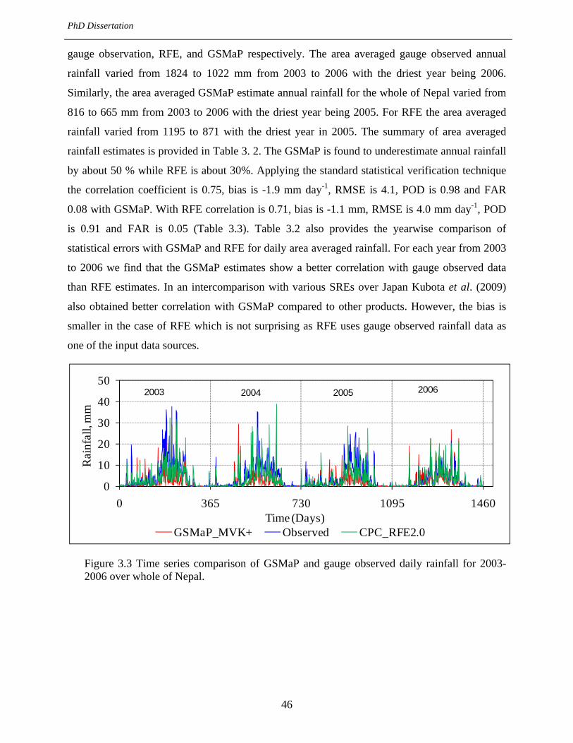
PhD Dissertation
46
gauge observation, RFE, and GSMaP respectively. The area averaged gauge observed annual
rainfall varied from 1824 to 1022 mm from 2003 to 2006 with the driest year being 2006.
Similarly, the area averaged GSMaP estimate annual rainfall for the whole of Nepal varied from
816 to 665 mm from 2003 to 2006 with the driest year being 2005. For RFE the area averaged
rainfall varied from 1195 to 871 with the driest year in 2005. The summary of area averaged
rainfall estimates is provided in Table 3. 2. The GSMaP is found to underestimate annual rainfall
by about 50 % while RFE is about 30%. Applying the standard statistical verification technique
the correlation coefficient is 0.75, bias is -1.9 mm day-1, RMSE is 4.1, POD is 0.98 and FAR
0.08 with GSMaP. With RFE correlation is 0.71, bias is -1.1 mm, RMSE is 4.0 mm day-1, POD
is 0.91 and FAR is 0.05 (Table 3.3). Table 3.2 also provides the yearwise comparison of
statistical errors with GSMaP and RFE for daily area averaged rainfall. For each year from 2003
to 2006 we find that the GSMaP estimates show a better correlation with gauge observed data
than RFE estimates. In an intercomparison with various SREs over Japan Kubota et al. (2009)
also obtained better correlation with GSMaP compared to other products. However, the bias is
smaller in the case of RFE which is not surprising as RFE uses gauge observed rainfall data as
one of the input data sources.
Figure 3.3 Time series comparison of GSMaP and gauge observed daily rainfall for 2003-2006 over whole of Nepal.
0
10
20
30
40
50
0 365 730 1095 1460
Rai
nfal
l, m
m
Time (Days)GSMaP_MVK+ Observed CPC_RFE2.0
2003 2004 2005 2006

PhD Dissertation
47
Table 3.2 Comparison of area averaged annual rainfall estimates over whole of Nepal using GSMaP and RFE
Year Annual Rainfall (mm) Percentage Error (%)
Observed GSMaP RFE GSMaP RFE
2003 1824.3 816.4 1195.3 -55 -33 2004 1570.8 703.4 1054.4 -55 -33 2005 1315.6 665.0 871.2 -49 -34 2006 1022.4 806.9 977.7 -21 -4 Average 1433.3 747.9 1024.7 -48 -29
Table 3.3 Time series comparison of daily area averaged rainfall from 2003 to 2006
Bias RMSE correl PE MBias POD FAR
2003: GSMaP -2.7 5.0 0.83 -54.7 0.45 1.00 0.08 RFE -1.7 4.6 0.79 -33.5 0.66 0.91 0.06
2004: GSMaP -2.4 4.5 0.73 -55.2 0.45 0.91 0.05 RFE -1.4 4.6 0.67 -32.9 0.67 0.89 0.03
2005: GSMaP -1.8 3.9 0.72 -49.2 0.51 1.00 0.12 RFE -1.2 3.6 0.72 -33.5 0.67 0.94 0.06
2006: GSMaP -0.6 2.4 0.81 -21.1 0.79 1.00 0.09 RFE -0.1 2.6 0.79 -4.4 0.96 0.89 0.05
Average: GSMaP -1.9 4.1 0.75 -47.6 0.52 0.98 0.08 RFE -1.1 4.0 0.71 -28.4 0.72 0.91 0.05
Spatial Distribution of Annual Precipitation
In addition to the area averaged annual rainfall variation understanding the spatial distribution of
rainfall is very important for various applications in water resources assessment as well as in
flood forecasting. In this section we seek to understand how closely the SREs conform to the
gauge observed rainfall and how good are they to represent the spatial variation. The analysis has
been conducted using the daily rainfall estimates of RFE, GSMaP and gauge observation for the
same period from 2003 to 2006.
In the gauge observed analysis precipitation is detected to be relatively heavy in central
Nepal near Pokhara exceeding 3000 mm/yr agreeing with Kansakar et al. (2004) and Ichiyanagi
et al. (2007). Kansakar et al. (2004) described zones of heavy precipitation also in the northeast
of the Kathmandu Valley which we can also see in the 2003 to 2006 gauge observed analysis.

PhD Dissertation
48
The highest annual precipitation amount is about 4500 mm in 2003 from the gauge observed
analysis which is quite close to the average amount referred in Chalise et al. (1996) despite the
short period of analysis from 2003 to 2006. The driest part of the country is the rain shadow area
of Mustang in the transhimalayan region with below 200 mm of rainfall similar to the Tibetan
plateau region.
The spatial distribution of average annual precipitation obtained from RFE and GSMaP are
also similar to that of the gauge observed and in general represents the spatial distribution of
rainfall well. However, there are distinct variations in the pattern in the mid mountain areas.
Figure 3.4 presents the comparison of spatial distribution of mean annual precipitation (SREs
using RFE and GSMaP and gauge observed rainfall) averaged from 2003 to 2006. Inspecting the
satellite-based rainfall analysis for 2003 we find that the highest annual precipitation amount is
about 2196 mm and 1798 mm from RFE and GSMaP respectively compared to 4500 mm with
gauge observed analysis. There is underestimation of the amount by both SREs. Further, it is
found that in the SREs the heavy precipitation tends to be more towards the southern belt rather
than in the mid mountain regions. This variation may be due to the orographic influence on
precipitation in the mid mountain areas which the SRE seem to not detect well. There are also
some local variations in pattern for example in the far eastern and western region of Nepal where
gauge observation shows higher precipitation while SREs seem to not capture this variation. The
observed trend is decrease in precipitation from east to west while this is not adequately reflected
in the SREs. The better quantitative estimate of RFE compared to GSMaP is quite likely because
the RFE estimate is gauge merged SREs and utilizes the WMO observed rainfall datasets while
the GSMaP is based on satellite observations only.

PhD Dissertation
49
( a )
( b )
( c )
Figure 3.4 Spatial distribution of average annual precipitation from 2003 to 2006, a) gauge observed, b) GSMaP and c) RFE

PhD Dissertation
50
Figure 3.5 presents the average annual rainfall bias map using GSMaP and RFE rainfall
estimates. As we have seen both the products are significantly underestimating the amount of
rainfall. However, it is interesting to observe the difference in the bias between the two products
GSMaP is found to have larger underestimation of rainfall in the central region compared to RFE
as seen in Figure 3.5. In the central north region in the trans-himalayas both products are found
to have positive bias though RFE has higher positive bias. In the central far east of Nepal
GSMaP and RFE have negative bias with GSMaP having higher negative bias.
(a) GSMaP
(b) RFE
Figure 3.5 Bias Map of average annual precipitation for 2003-2006, a) GSMaP and b) RFE

PhD Dissertation
51
Figure 3.6 presents the spatial distribution of average annual precipitation year wise from
2003 to 2006 for GSMaP, RFE and gauge observed rainfall. For every year SREs using RFE and
GSMaP underestimates the annual precipitation.
2003: GSMaP
2003: RFE
2003: Gauge Observed
2004: GSMaP
2004: RFE
2004: Gauge Observed
2005: GSMaP
2005: RFE
2005: Gauge Observed
2006: GSMaP
2006: RFE
2006: Gauge Observed
Figure 3.6 Spatial distribution of annual precipitation with GSMaP, RFE and gauge observed rainfall for 2003 to 2006

PhD Dissertation
52
2003: GSMaP Bias Map
2003: RFE Bias Map
2004: GSMaP Bias Map
2004: RFE Bias Map
2005: GSMaP Bias Map
2005: RFE Bias Map
2006: GSMaP Bias Map
2006: RFE Bias Map
Figure 3.7 Annual bias map for each year from 2003 to 2006 with GSMaP and RFE
Figure 3.7 presents the bias map of average annual precipitation showing yearly variation in
the bias. In general the positive and negative biases for both satellite-based products are similar
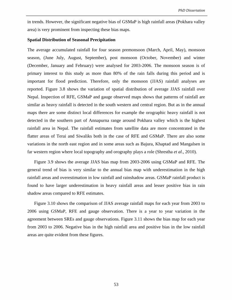
PhD Dissertation
53
in trends. However, the significant negative bias of GSMaP is high rainfall areas (Pokhara valley
area) is very prominent from inspecting these bias maps.
Spatial Distribution of Seasonal Precipitation
The average accumulated rainfall for four season premonsoon (March, April, May), monsoon
season, (June July, August, September), post monsoon (October, November) and winter
(December, January and February) were analysed for 2003-2006. The monsoon season is of
primary interest to this study as more than 80% of the rain falls during this period and is
important for flood prediction. Therefore, only the monsoon (JJAS) rainfall analyses are
reported. Figure 3.8 shows the variation of spatial distribution of average JJAS rainfall over
Nepal. Inspection of RFE, GSMaP and gauge observed maps shows that patterns of rainfall are
similar as heavy rainfall is detected in the south western and central region. But as in the annual
maps there are some distinct local differences for example the orographic heavy rainfall is not
detected in the southern part of Annapurna range around Pokhara valley which is the highest
rainfall area in Nepal. The rainfall estimates from satellite data are more concentrated in the
flatter areas of Terai and Siwaliks both in the case of RFE and GSMaP. There are also some
variations in the north east region and in some areas such as Bajura, Khaptad and Mangalsen in
far western region where local topography and orography plays a role (Shrestha et al., 2010).
Figure 3.9 shows the average JJAS bias map from 2003-2006 using GSMaP and RFE. The
general trend of bias is very similar to the annual bias map with underestimation in the high
rainfall areas and overestimation in low rainfall and rainshadow areas. GSMaP rainfall product is
found to have larger underestimation in heavy rainfall areas and lesser positive bias in rain
shadow areas compared to RFE estimates.
Figure 3.10 shows the comparison of JJAS average rainfall maps for each year from 2003 to
2006 using GSMaP, RFE and gauge observation. There is a year to year variation in the
agreement between SREs and gauge observations. Figure 3.11 shows the bias map for each year
from 2003 to 2006. Negative bias in the high rainfall area and positive bias in the low rainfall
areas are quite evident from these figures.

PhD Dissertation
54
(a) Gauge Observed
(b) GSMaP
(c) RFE
Figure 3.8 Spatial distribution of June, July, August and September (JJAS) average rainfall map for 2003-2006 a) gauge observed, b) GSMaP and c) CPC_RFE2.0.

PhD Dissertation
55
(a) Bias with GSMaP
(b) Bias with RFE
Figure 3.9 Bias Map of average JJAS precipitation for 2003-2006, a) GSMaP and b) RFE

PhD Dissertation
56
2003: GSMaP 2003: RFE
2003: Gauge Observed
2004: GSMaP
2004: RFE
2004: Gauge Observed
2005: GSMaP
2005: RFE 2005: Gauge Observed
2006: GSMaP
2006: RFE
2006: Gauge Observed
Figure 3.10 Spatial distribution of year wise average JJAS rainfall using GSMaP, CPC_RFE2.0 and gauge observation over Nepal for 2003 to 2006.

PhD Dissertation
57
2003: Bias GSMaP
2003: Bias RFE
2004: Bias GSMaP
2004: Bias: GSMaP
2005: Bias GSMaP
2005: Bias RFE
2006: Bias GSMaP
2006: Bias RFE
Figure 3.11 Bias Map of JJAS precipitation for 2003-2006, a) GSMaP and b) RFE

PhD Dissertation
58
Scatter plots of area averaged daily rainfall for the monsoon (JJAS) for 2003 to 2006 for
GSMaP and RFE estimates are shown in Figure 3.12. For the area averaged daily rainfall for the
period 2003 to 2006 the correlation coefficient is 0.79, bias is -5.0 mm day-1, and RMSE is 5.6
for GSMaP and 0.72, -2.9 mm day-1 and RMSE is 4.0 mm for RFE respectively (Table 3.4). The
bias is less in the RFE estimates than the GSMaP, however, the GSMaP has a higher correlation
coefficient.
(a)
(b)
Figure 3.12 Scatter plot of area averaged daily rainfall for monsoon (JJAS) of 2003-2006 from a) observed and GSMaP, (b) observed and RFE.
Table 3.4 Statistical error of daily area average rainfall from 2003-2006 for JJAS
Bias RMSE PE correl MBias POD FAR
RFE -2.9 4.0 -31.9 0.72 0.68 1.00 0.00 GSMaP -5.0 5.6 -54.1 0.79 0.46 1.00 0.00
Figure 3.13 shows the scatter plot of average accumulated rainfall for each 0.1o x 0.1o grid
cell (862 grid cells in total) for JJAS for 2003 to 2006 for GSMaP and RFE estimates. For the
average accumulated monsoon rainfall (JJAS) of each 0.1o x 0.1o grid cell the correlation
coefficient is 0.46, bias is -609.7 mm and RMSE is 736.5 with a percentage error of -54.2% for
GSMaP and 0.35, -352.0 mm, 569.8, -31.3% for RFE respectively. Table 3.5 shows that the bias
is less in the RFE estimates than the GSMaP, however, the GSMaP has a higher correlation
coefficient. The underestimation of rainfall is consistent with previous finding (Shrestha et al.,
2008; Dinku et al., 2008; Ebert et al., 2007a). In the case of Ethiopia, with a complex terrain
similar to the study area, Dinku et al. (2008) investigated the performance of various satellite
y = 1.2232x + 4.0513R² = 0.6194
0.0
5.0
10.0
15.0
20.0
25.0
30.0
0.0 5.0 10.0 15.0 20.0 25.0 30.0
Obs
erve
d R
ainf
all (
mm
)
GSMap_MVK+ estimated Rainfall (mm)
Total points = 122 days
y = 0.8947x + 3.6034R² = 0.5116
0.0
5.0
10.0
15.0
20.0
25.0
30.0
0.0 5.0 10.0 15.0 20.0 25.0 30.0O
bser
ved
Rai
nfal
l (m
m)
CPC_RFE2.0 estimated Rainfall (mm)
Total points = 122 days

PhD Dissertation
59
rainfall products and found that satellite-based estimates did well in detecting the occurrence of
rainfall, but were not good in estimating the amount of daily rainfall. Table 3.5 presents the
statistical error of accumulated rainfall for monsoon (JJAS) from 2003-2006 at each grid cell.
(a)
(b)
Figure 3.13 Scatter plot of accumulated average rainfall for JJAS of 2003-2006 from a) GSMaP and b) CPC_RFE2.0for each 0.1ox0.1o grid cell.
Table 3.5 Statistical error of accumulated rainfall for monsoon (JJAS) from 2003-2006 at each grid cell
Bias RMSE PE correl MBias POD FAR
RFE -352.0 569.8 -31.3 0.35 0.69 1.0 0.0 GSMaP -609.7 736.5 -54.2 0.46 0.46 1.0 0.0
The monthly, seasonal and annual total rainfall is computed from the daily analyzed values.
The year 2003 is selected over the whole observation period as 2003 is the wettest year and
SREs from GSMaP. Using the 0.1ox0.1o data set of individual grids the total annual rainfall in
2003 is 1824.3 mm from gauge and 816.4 mm from the GSMaP. There is a negative bias of
1007.9 mm year-1 (Table 3.6). During the monsoon (JJAS) there is an accumulated rainfall of
1501.8 mm from gauge and 605.3 mm from GSMaP with a highest negative bias of 896.5 mm
compared to other seasons. The correlation coefficient between the gauge observed and the
GSMaP annual rainfall estimates is 0.48 and for the monsoon is 0.47 (Shrestha et al., 2010).
0
500
1000
1500
2000
2500
3000
0 500 1000 1500 2000 2500 3000
Obs
erve
d R
ainf
all (
mm
)
GSMap_MVK+ estimated Rainfall (mm)
Total points = 862 grid cells
0
500
1000
1500
2000
2500
3000
0 500 1000 1500 2000 2500 3000
Obs
erve
d R
ainf
all (
mm
)
CPC_RFE2.0 estimated Rainfall (mm)
Total points = 862 grid cells
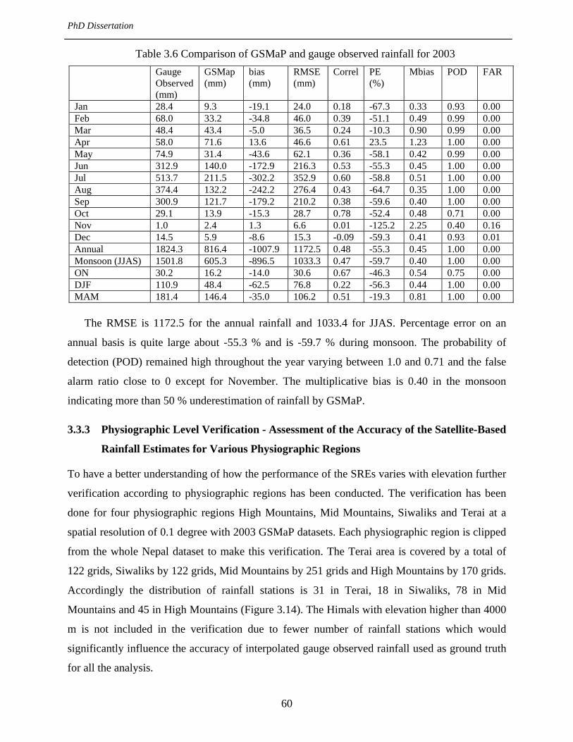
PhD Dissertation
60
Table 3.6 Comparison of GSMaP and gauge observed rainfall for 2003
The RMSE is 1172.5 for the annual rainfall and 1033.4 for JJAS. Percentage error on an
annual basis is quite large about -55.3 % and is -59.7 % during monsoon. The probability of
detection (POD) remained high throughout the year varying between 1.0 and 0.71 and the false
alarm ratio close to 0 except for November. The multiplicative bias is 0.40 in the monsoon
indicating more than 50 % underestimation of rainfall by GSMaP.
3.3.3 Physiographic Level Verification - Assessment of the Accuracy of the Satellite-Based
Rainfall Estimates for Various Physiographic Regions
To have a better understanding of how the performance of the SREs varies with elevation further
verification according to physiographic regions has been conducted. The verification has been
done for four physiographic regions High Mountains, Mid Mountains, Siwaliks and Terai at a
spatial resolution of 0.1 degree with 2003 GSMaP datasets. Each physiographic region is clipped
from the whole Nepal dataset to make this verification. The Terai area is covered by a total of
122 grids, Siwaliks by 122 grids, Mid Mountains by 251 grids and High Mountains by 170 grids.
Accordingly the distribution of rainfall stations is 31 in Terai, 18 in Siwaliks, 78 in Mid
Mountains and 45 in High Mountains (Figure 3.14). The Himals with elevation higher than 4000
m is not included in the verification due to fewer number of rainfall stations which would
significantly influence the accuracy of interpolated gauge observed rainfall used as ground truth
for all the analysis.
Gauge Observed (mm)
GSMap (mm)
bias (mm)
RMSE (mm)
Correl PE (%)
Mbias POD FAR
Jan 28.4 9.3 -19.1 24.0 0.18 -67.3 0.33 0.93 0.00 Feb 68.0 33.2 -34.8 46.0 0.39 -51.1 0.49 0.99 0.00 Mar 48.4 43.4 -5.0 36.5 0.24 -10.3 0.90 0.99 0.00 Apr 58.0 71.6 13.6 46.6 0.61 23.5 1.23 1.00 0.00 May 74.9 31.4 -43.6 62.1 0.36 -58.1 0.42 0.99 0.00 Jun 312.9 140.0 -172.9 216.3 0.53 -55.3 0.45 1.00 0.00 Jul 513.7 211.5 -302.2 352.9 0.60 -58.8 0.51 1.00 0.00 Aug 374.4 132.2 -242.2 276.4 0.43 -64.7 0.35 1.00 0.00 Sep 300.9 121.7 -179.2 210.2 0.38 -59.6 0.40 1.00 0.00 Oct 29.1 13.9 -15.3 28.7 0.78 -52.4 0.48 0.71 0.00 Nov 1.0 2.4 1.3 6.6 0.01 -125.2 2.25 0.40 0.16 Dec 14.5 5.9 -8.6 15.3 -0.09 -59.3 0.41 0.93 0.01 Annual 1824.3 816.4 -1007.9 1172.5 0.48 -55.3 0.45 1.00 0.00 Monsoon (JJAS) 1501.8 605.3 -896.5 1033.3 0.47 -59.7 0.40 1.00 0.00 ON 30.2 16.2 -14.0 30.6 0.67 -46.3 0.54 0.75 0.00 DJF 110.9 48.4 -62.5 76.8 0.22 -56.3 0.44 1.00 0.00 MAM 181.4 146.4 -35.0 106.2 0.51 -19.3 0.81 1.00 0.00

PhD Dissertation
61
Figure 3.14 Location of rainfall stations in various physiographic regions of Nepal
Table 3.7 presents the comparison of annual GSMaP and gauge observed rainfall in the four
physiographic regions of Nepal. In the Terai and Siwaliks area where the elevation is fairly low
less than 1500 m the correlation coefficient between the GSMaP and gauge observed rainfall is
high above 0.8. In the Mid Mountains and High Mountain areas where orography plays an
important role the correlation coefficient decreases to about 0.4 on average with increasing
RMSE. In the High Mountains the RMSE is 1470.1 and in the Mid Mountains 1070.4. Despite
the relatively denser network of rainfall stations the prediction in the Mid Mountain area is less
than in the Terai and Siwaliks. The percentage error an indicator of how close the predictions are
to observed values also is minimum in the Terai (-38.8%) and maximum in the High Mountains
(-67.4%). The correlation coefficient is highest in the Siwlaki (0.85) and Terai (0.84) regions
while it decreases to 0.83 in the mid mountain region and to 0.47 in the High mountains. The
multiplicative bias is higher in the Terai and Siwalik region and decreases rapidly to less than 0.4
in the High mountains indicating the performance of satellite based rainfall estimates to
deteriorate with higher altitude region where influences of orography is high. The accuracy of
prediction in the Terai and Siwalik is about 38% while with increase in elevation this accuracy

PhD Dissertation
62
decreases to 49% in the middle mountains and more than 67% in the high mountain regions
(Shrestha et al., 2010).
Table 3.7 Error statistics of area averaged annual GSMaP and gauge observed rainfall in various physiographic regions for 2003.
Table 3.8 Error statistics of monsoon (JJAS) GSMaP and gauge observed rainfall in physiographic regions for 2003.
For the monsoon (JJAS) similar results are obtained as shown in Table 3.8. The correlation
coefficient is high in the Siwaliks and Terai region on an average of about 0.8 while in the
Middle and High Mountain region the correlation coefficient sharply drops to about 0.4. The
RMSE is lowest in the Terai (697.2) and highest in the High Mountains (1277.9). This result
clearly illustrates that GSMaP performs well in the flatter terrain with better prediction (Shrestha
et al., 2010). While with increasing elevation the accuracy of predicting rainfall by GSMaP
algorithm is found to become lower. Worse performances of the SREs over mountainous regions
of Japan were indicated by previous works (Kubota et al., 2009; Shiraishi et al., 2009). This may
be due to the impact of orographic enhancement of rainfall despite denser network of stations in
the Mid Mountain region. The GSMaP uses a statistical database of precipitation vertical profiles
classified into 10 types (Aonashi et al., 2009), but currently it cannot reflect profiles of localized
precipitation systems. The profiles of heavy orographic rainfall are unique and largely different
from those in the database, which can lead to large errors (Kutota et al., 2009).
Table 3.9 shows the error statistics of daily area averaged GSMaP and gauge observed
rainfall during JJAS in various physiographic regions. Similar to the accumulated rainfall
comparison the correlation is high in the Terai and Siwalik regions and reduces significantly in
bias
RMSE
Correl
PE
Mbias
POD
FAR
Terai -743.4 784.6 0.80 -38.8 0.61 1.00 0.00 Siwaliks -697.6 764.7 0.88 -37.0 0.63 1.00 0.00
Mid Mountains -931.9 1070.4 0.37 -49.0 0.51 1.00 0.00 High Mountains -1313.1 1470.1 0.43 -67.4 0.33 1.00 0.00
bias
RMSE
Correl
PE
Mbias
POD
FAR
Terai -662.4 697.2 0.76 -41.4 0.59 1.00 0.00 Siwaliks -645.9 721.8 0.83 -40.9 0.59 1.00 0.00
Mid Mountains -832.5 943.3 0.40 -53.0 0.47 1.00 0.00 High Mountains -1151.1 1277.9 0.46 -72.5 0.27 1.00 0.00

PhD Dissertation
63
the High Mountains. The error in detection is also lowest in the Terai and Siwalki region and
increases to about 70% in the High Mountains. The daily bias in the Siwalik is half of that of the
High Mountain region.
Table 3.9 Error statistics of daily GSMaP and gauge observed rainfall during JJAS in various physiographic regions for 2003.
RMSE Correl PE Mbias POD FAR
Terai -2.0 5.5 0.84 -38.0 0.62 0.73 0.01 Siwaliks -1.8 5.1 0.85 -35.9 0.64 0.73 0.00 Mid Mountains -2.5 5.1 0.83 -48.3 0.52 0.70 0.01 High Mountains -3.6 6.8 0.47 -67.0 0.33 1.00 0.12
Figure 3.15 illustrates the scatter plot of accumulated rainfall for JJAS of 2003 from
observed and GSMaP for each grid cell. The poor performance of SREs in the high mountains is
quite evident. We see that the High mountain regions show greater underestimation of rainfall
compared to Siwalik and Terai regions. It is quite clear from this analysis that at higher elevation
where orographic influence is evident the performance of the SREs decreases. However, the
decrease in the performance cannot be solely attributed to orography only because other factors
such as wind, slope and aspect are also important. Figure 3.16 shows the scatter plots of area
averaged rainfall for the various physiographic regions of Nepal.

PhD Dissertation
64
Figure 3.15 Scatter plot of accumulated rainfall for JJAS of 2003 from observed and GSMaP for each 0.1ox0.1o grid cell.
0
500
1000
1500
2000
2500
3000
3500
4000
0 1000 2000 3000 4000
Obs
erve
d R
ainf
all (
mm
)
GSMap_MVK+ estimated Rainfall (mm)High Mountain Siwalik Terai Mid Mountains

PhD Dissertation
65
Terai
Siwalik
Middle Mountains High Mountains
Figure 3.16 Scatter plots of area averaged rainfall for various physiographic regions of Nepal
3.3.4 Basin Level Verification in the Bagmati and Narayani Basins
There are three major river basins in Nepal the Koshi, Narayani and the Karnali. Apart from
these river basins there are other river basins like Bagmati, East Rapti as shown in Figure 3.17.
For the current research, basin level verification has been done for two basins Bagmati and
Narayani. These two basins were selected to study the performance of SRE considering the flood
vulnerability of the basin as well as the catchment sizes and topographic extent. Narayani Basin
is a snow fed basin with more than 15 % of catchment area above 5000 m while the Bagmati
Basin is below 2700 m with a catchment area of 2800 km2. However, in both the basin flooding
y = 1.1466x + 1.3388R² = 0.7269
0
10
20
30
40
50
60
70
80
0 20 40 60 80
Obs
erve
d R
ainf
all (
mm
)
GSMap MVK+ Rainfall Estimate (mm)
y = 1.1776x + 1.4076R² = 0.6989
0
10
20
30
40
50
60
0 10 20 30 40 50 60
Obs
erve
d R
ainf
all (
mm
)
GSMap MVK+ Rainfall Estimate (mm)
y = 1.1997x + 1.9704R² = 0.6815
0
5
10
15
20
25
30
35
40
45
50
0 10 20 30 40 50
Obs
erve
d R
ainf
all (
mm
)
GSMap MVK+ Rainfall Estimate (mm)
y = 0.9824x + 3.5934R² = 0.2189
0
5
10
15
20
25
30
0 5 10 15 20 25 30
Obs
erve
d R
ainf
all (
mm
)
GSMap MVK+ Rainfall Estimate (mm)

PhD Dissertation
66
causes adverse impacts to people’s lives and livelihoods on a regular basis. It is anticipated that
the study of these two basins will enable a better understanding of the performance of SREs for
flood prediction purposes. The characteristics of the two basins are provided in Table 3.10.
Figure 3.17 Major river basins of Nepal
Table 3.10 Characteristics of Bagmati and Narayani Basins
Bagmati Narayani
Catchment Area [km2] 2800 (at Pandheradovan) 32000 (at Devghat) Altitudinal range [m] 70 – 2700 100 - >8000 Physiography Terai, Siwalik and Middle
mountains (alluvial plain to the mid mountains)
Terai, Siwaliks, Middle mountains, High Mountains and Himal (alluvial plain to the himal with tundra conditions)
Dominant land use Forest and agriculture Forest and agriculture Annual rainfall [mm] 1800 2000 Range of annual rainfall[mm] 1200 - 2000 200 - 6000
Bagmati Basin
The Bagmati Basin originates in the Mahabhararat range of the Middle Mountains of Nepal at
elevation of around 2700 m and drains southward into the state of Bihar in India to join the
Ganges River. It has a catchment area of about 3550 km2 upto the Nepal India border and has

PhD Dissertation
67
been classified into three physiographic regions. The upper part of the Bagmati Basin covers the
whole of Kathmandu Valley. The middle part of the catchment extends downstream of the
Chovar gorge to the Terai area at Pandhera Dovan near Karmaiya where the catchment area is
about 2800 km2. Further downstream beyond Pandhera Dovan gauging station the river then
flows through the third part of the catchment with the lowest elevation of the Bagmati River at
the Nepal India border at about 70 m above mean sea level (Figure 3.18). The catchment area of
the Bagmati Basin lying below 1000 m inside Nepal is about 2050 km2 and that lying between
1000 m and 3000 m is about 1500 km2. The location of the basin is shown in Figure 3.17. The
average elevation of the basin is about 1350 m. The total length of the river from its origin to
Nepal India border is 170 km. The average slope of the river is about 1% which flattens down to
0.03% in the Terai area. The catchment lies in eight districts of Nepal; Kathmandu, Lalitpur,
Bhaktapur, Sindhuli, Kavre, Makwanpur, Rautahat, and Sarlahi.
Figure 3.18 Location of rainfall station in the Bagmati Basin and its vicinity
and discharge gauging station at Pandhera Dovan
Assessment of the accuracy of the RFE estimates
The rainfall observed at the rain gauge stations was higher than the concurrent RFE. Figure 3.19
shows an example of a rainfall event on July 23, 2002 along with the details of the statistical
analysis. The probability of detection is 1 and the false alarm ratio is 0 showing that the RFE is
capturing the rainfall event quite well qualitatively in terms of occurrence. However, the
Pandhera Dovan

PhD Disse
estimated
shows th
to Augus
However
when th
illustratin
Figu
ertation
d rainfall is
he compariso
st 7, 2002.
r, the RFE a
e rain gaug
ng the rando
ure 3.19 Com
lower than
on of the gau
The RFE ca
almost comp
ges network
om errors in t
mparison of r
n the observ
uge observed
aptures the r
pletely miss t
k showed t
the RFE (Sh
rain gauge o
68
ved amount
d rainfall and
rainfall tren
to register a
he second
hrestha et al.
observed and2002
indicating a
d RFE for th
nds well but
any significa
highest rain
, 2008).
d RFE for the
a negative b
he 38 days pe
underestim
ant rainfall o
nfall amoun
e Bagmati B
bias. Figure
eriod from J
mates the am
on day 204, a
nt of the p
Basin on July
3.20
July 1
mount.
a day
period
y 23,

PhD Dissertation
69
Figure 3.20 Basin average rainfall of Bagmati Basin for 2002
The daily accuracy of RFE was determined comparing the daily basin average rainfall for
June, July, August and September (JJAS) from 2002 to 2006 (Figure 3.21). Table 3.11 provides
the yearwise statistics of the performance of RFE compared to the gauge observed data of daily
basin average rainfall. The correlation coefficient between the RFE and gauge observed daily
basin average rainfall for JJAS was found to vary from 0.49 to 0.68 for each year with an
average correlation of 0.60. The daily area averaged bias is -3.6 mm, RMSE is 13.1 mm and
percentage error is -30.7 for the period 2002 to 2006. Figure 3.21 illustrates the underestimation
of daily basin average rainfall from RFE compared to gauge observed rainfall for JJAS from
2002 to 2006. A histogram of daily basin averaged rainfall for 2003 is shown in Figure 3.22. The
RFE showed relatively good agreement on some days while on other days, the RFE completely
failed to register any significant rainfall when the rain gauge network showed high rainfall
amounts.
020406080
100120140160180200
182 187 192 197 202 207 212 217Days
Rai
nfal
l (m
m)
Gauge observed rain RFE

PhD Dissertation
70
Figure 3.21Time series comparison of gauge observed and RFE daily basin average rainfall for
monsoon (JJAS) from 2002 to 2006 in the Bagmati Basin
Table 3.11Statistics of performance of daily RFE compared to gauge observed data for JJAS from 2002 to 2006
Figure 3.22 Daily basin averaged gauge observed rainfall with RFE for JJAS of 2003 in the Bagmati Basin
020406080
100120140160
Rai
nfal
l (m
m)
RFE Observed
2002 2003 2004 2005 2006
0102030405060708090
100
152 162 172 182 192 202 212 222 232 242 252 262 272
Rai
nfal
l (m
m)
Time (Days)
RFE Gauge Observed
Year B ias (mm/day)
RMSE (mm/day)
r PE (%)
Mbias
2002 -5.4 14.9.9 0.68 -39.1 0 .61 2003 -4.2 13.5 0.58 -31.2 0.69 2004 -2.1 16.3 0.49 -18.8 0.81 2005 -4.3 10.3 0.64 -42.7 0.57 2006 -1.8 8.7 0.63 -19.3 0.81
Av erage (2003-2006) -3.6 13.1 0.60 -30.7 0.69

PhD Dissertation
71
Narayani Basin
The Narayani Basin lies in the Western Development Region of Nepal (Figure 3.17). The
Narayani river system has five major tributaries, the Kali Gandaki, Seti Gandaki, Marsyandi,
Budhi Gandaki, and Trisuli. The Trisuli and Budhi Gandaki originate in the Tibet Autonomous
Region of China, while the other three originate within Nepal. The Kali Gandaki is the main
river in this drainage system. After the confluence of its five tributaries, the Narayani flows
through Devghat and meets the Ganges in India. Geographically, it is located between longitudes
82.88o to 85.70o east and latitudes 27.36o to 29.33o north and passes through 19 districts of
Nepal. It has a total drainage area of 32,000 km2 at the Devghat hydrometric station.
The basin has high topographic variation with elevation ranging from 60 m in the south to
higher than 8000 m in the north where it passes through the high Himalayas, which contain the
Dhaulagiri (8167 m) and Annapurna (8091 m) peaks. The Narayani Basin contains all five
physiographic regions of Nepal: the Terai (the northward extension of Indo-Gangetic plain), the
Siwalik (Chure Hills), Middle Mountains, High Mountains, and Himal. The Terai covers an area
extending from an altitude of less than 500 m (9.2%), the Siwaliks from 501 to 1500 m (31.1%),
the Middle Mountains from 1501 to 3,000 m (18.2%), High Mountains from 3001 to 5000 m
(26.5%) and Himals above 5000 m (14.9%). Given the topographic variation the climate varies
from subtropical in the Terai to alpine conditions in the Himal. There is pronounced temporal
and spatial variation in precipitation in the basin; the mean annual precipitation varies from 200
mm to more than 5000 mm (Sharma, 1977; Chalise et al., 1996). The upper basin of the Kali
Gandaki lies in the Trans Himalayan region, which has arid conditions. The main rainy season is
the monsoon from June to September.
The Narayani Basin is one of major development hubs of Nepal contributing about 50 per
cent of the total hydropower production of the country (NEA, 2008). In 1993, a large flood
occurred in the Narayani Basin with record high rainfall of 540 mm in 24 hours and intensity
exceeding 70 mm/hr, during which more than 1050 people lost their lives. Bhusal and Bhattarai
(2002) noted that had there been a flood forecasting system in place the loss of lives would have
been minimized. Hence, SREs now available at a higher resolution provides an opportunity for
flood prediction.

PhD Dissertation
72
Assessment of the accuracy of the RFE estimates
Verification of the RFE rainfall estimates over the Narayani Basin was conducted by comparing
with the gauge observed rainfall data for selected high rainfall days from 2003 and 2004. The
Narayani Basin is covered by 234 grids of 0.1 degree resolution; 41 of the grids contain one or
more rainfall stations (Figure 3.23). Comparison of the gauge observed and estimated rainfall in
those grids with one or more stations shows that, on average, the observed rainfall was higher
than the concurrent rainfall estimates in all cases considered. Figure 3.23 shows an example of a
rainfall event on 9 July 2003, along with the statistics.
The RFE captures the rainfall spatial trends well, but underestimates the amount on average
by more than 50 per cent. The POD was 0.97 and the FAR was 0.05. The RMSE was 45.2 mm;
using the Wilmott method (Wilmott, 1982; Wilmott et al., 1985), 34.7 mm was unsystematic
RMSE (0.59), and 28.9 mm was systematic RMSE (0.41). The RFE estimated rainfall was lower
than the gauge observed rainfall amount with bias of 33.7 mm. The random and systematic errors
observed in the RFE estimates result from the uncertainty in estimates from the individual data
sources used to produce the RFE product (Xie et al., 2002). The satellite data used in the
production of the RFE are from microwave imagers and infrared imagery. The SSM/I and
AMSU-B are the primary passive microwave data included in the RFE estimates. These data
have a strong physical relationship to the hydrometeors that result in surface precipitation, but
each individual satellite provides a very sparse sampling of the time-space occurrence of
precipitation (Huffman et al., 2007). The random error observed in the rainfall estimates could
partly be associated with this limited sampling of satellite observations.

PhD Dissertation
73
Figure 3.23 Comparison of gauge observed and RFE for 9 July, 2003 in the Narayani Basin
The daily accuracy of RFE was determined comparing the daily basin average rainfall for
June, July, August and September (JJAS) from 2002 to 2006 (Figure 3.24). Table 3.12 provides
the yearwise statistics of the performance of RFE compared to the gauge observed data of daily
basin average rainfall. The correlation coefficient between the RFE and gauge observed daily
basin average rainfall for JJAS was found to vary from 0.40 to 0.69 for each year with an
average correlation of 0.50. The daily basin averaged bias is -4.9 mm, RMSE is 8.8 mm and
percentage error is -43.4 for the period 2002 to 2006. Figure 3.25 illustrates the underestimation
of daily basin average rainfall from RFE compared to gauge observed rainfall for JJAS from
2002 to 2006. A histogram of daily basin averaged rainfall for 2003 is shown in Figure 3.25. The
RFE showed relatively good agreement on some days while on other days, the RFE completely
Contingency Table
37 21 1
Probability of Detection (POD) 0.97False Alarm Ratio (FAR) 0.05Mean Absolute Error (MAE) 36.1Bias -33.7Root Mean Square Error (RMSE) 45.2Correlation Coefficient 0.60
-62.1
Est
imat
ed
Rai
nfal
l
Percentage Error
Observed Rainfall
Gauge observed rainfall (mm)
Low: 0 High: 129
CPC_RFE2.0 rainfall estimates (mm)
Low: 0 High: 74

PhD Dissertation
74
failed to register any significant rainfall when the rain gauge network showed high rainfall
amounts. This random nature of the SRE was also noted in the Bagmati Basin.
In both the basins there is a consistent underestimation of rainfall by RFE except for some
days where the satellite-based rainfall exceeds the gauge observed rainfall and shows false
detection. The bias is smaller in the Bagmati Basin compared to the Narayani. However, the
percentage error in the Narayani is larger than that observed in the Bagmati, suggesting that the
SREs perform better in the basins located in the Terai and Siwalik regions compared to basins
with substantial area in the Mid Mountain and High Mountain areas. The underestimation of
rainfall is consistent with previous studies (Dinku et al., 2008; Ebert et al., 2007; Harris et al.,
2007; Shrestha et al., 2008; Hughes, 2006). This underestimation of rainfall in the Narayani
Basin, may be further attributed to the orographic effects prevalent in the basin where rainfall
varies in small spatial scales between 200 mm to over 5000 mm which may not be adequately
represented in the current rain profile algorithms of the SRE. To accurately predict floods the
RFE thus needs to be adjusted.
Table 3.12 Statistics of performance of daily RFE compared to gauge observed data for JJAS from 2002 to 2006.
Year Bias (mm/day)
RMSE (mm/day)
r PE (%)
Mbias
2002 -6.7 12.0 0.41 -51.6 0.48 2003 -5.9 8.7 0.69 -44.2 0.56 2004 -5.7 8.9 0.40 -49.5 0.50 2005 -4.2 7.1 0.55 -46.2 0.54 2006 -2.1 6.7 0.50 -23.8 0.76
Average (2003-2006) -4.9 8.8 0.50 -43.4 0.57

PhD Dissertation
75
Figure 3.24 Time series comparison of gauge observed and RFE daily basin average rainfall for monsoon (JJAS) from 2002 to 2006 in the Narayani Basin
Figure 3.25 Daily basin averaged gauge observed rainfall with RFE for JJAS of 2003 in the Narayani Basin
3.4 Summary
Verification of SREs using two products, the RFE and GSMaP has been conducted at three
levels. The first set of verification was conducted at a country level. The GSMaP estimates were
found to underestimate the annual rainfall by 48 % and RFE by 30%. The GSMaP however
showed better correlation with the observed data as compared to RFE. The second level of
verification was conducted for various physiographic regions to assess the performance of RFE
0.0
10.0
20.0
30.0
40.0
50.0
60.0
Rai
nfal
l (m
m)
RFE Observed
2002 2003 2004 2005 2006
0
10
20
30
40
50
60
152 162 172 182 192 202 212 222 232 242 252 262 272
Rai
nfal
l (m
m)
Time (Days)
RFE Gauge Observed

PhD Dissertation
76
is various regions. Both SREs performed better in the flatter regions in the Terai and Siwalik
regions. The performance deteriorated with higher elevations with the minimum performance in
the High Mountain region. The middle mountain regions despite the dense network of stations
showed poorer performance of SREs. Finally, verification was also conducted at a basin level in
two basins Bagmati and Narayani which differ in catchment areas and general characteristics. On
a daily basis the Bagmati Basin has a lower bias than the Narayani. The percentage error is also
smaller in the Bagmati compared with the Narayani, suggesting that RFE performs better in
basins lying in the Siwaliks and the Terrai region compared to the Middle Mountains and High
Mountain areas. In all three levels of verification the SREs were found to be generally lower
than the gauge observed data indicating the need to adjust the rainfall estimates for further
application.
References
Aonashi, K., Awaka, J., Hirose, M., Kozu, T., Kubota, T., Liu, G., Shige, S., Kida, S., Seto, S.,
Takahashi, N., and Takayabu, Y. N.: GSMaP passive, microwave precipitation retrieval
algorithm: Algorithm description and validation. J. Meteor. Soc., Japan, Vol.87A, pp. 119-
136, 2009.
Basistha, A.; Arya, D. S.; Goel. N.K. (2007) Spatial Distribution of Rainfall in Indian Himalayas
– A Case Study of Uttarakhand Region, Water Resour Manage DOI 10.1007/s11269-007-
9228-2.
Chalise, S.R., Shrestha, M.L., Thapa, K.B., Shrestha, K.B., Bajracharya, B. (1996) Climatic and
hydrological Atlas of Nepal. Kathmandu: ICIMOD
Creutin, J.D., Obled, C. (1982) Objective analysis and mapping techniques for rainfall fields: an
objective comparison. Water Resour. Res. 18 2, pp. 251–256.
Diodato, N.; Ceccarelli, M. (2005) Interpolation processes using multivariate geostatistics for
mapping of climatological precipitation mean in the Sannio Mountains (southern Italy).
Earth Surf. Process. Landforms 30, pp. 259–268
Ebert, E.E. (2007a) Methods for verifying satellite-based precipitation estimates Measuring
Precipitation from Space, V. Levizzani et al. (eds) Eurainsat and the Future, pp. 345-356.

PhD Dissertation
77
Ebert, E.E.; Janowiak, J.E.; Kidd, C. (2007b) Comparison of near-real-time precipitation
estimates from satellite observations and numerical models. Bull. Amer. Meteorol. Soc. 88(1),
47–64.
Ebert, E.E.; McBride, J.L. (2000) Verification of precipitation in weather systems:
Determination of systematic errors. J. Hydrology, 239, 179-202.
Hughes, D.A. (2006) Comparison of satellite rainfall data with observation from gauging station
networks. J. Hydrol. 327, pp. 399-410.
Ichiyanagi, K.; Manabu, D.;Yoshitaka, Y.; Murajic, Y.; Vaidya, B.K. (2007) Precipitation in
Nepal between 1987 and 1996 International Journal of Climatology. 27, pp. 1753–1762
Isaaks, E. H., Srivastava, R.M. (1989) An Introduction to Applied Geostatistics. Oxford Univ.
Press, New York, Oxford. Kansakar, S.R.; Hannah, D.M.; Gerraed, J.; Rees, G. (2004) Spatial pattern in the precipitation
regime of Nepal. International Journal of Climatology 24, 1645–1659.
Kubota, T.; Ushio, T.; Shige, S.; Kachi, M.; Okamoto, K. (2009) Verification of high resolution
SRE around Japan using a gauge-calibrated ground-radar dataset. J. Meteorol. Soc., Japan
87A, pp. 203–222.
Shiraishi, Y., Fukami, K., Inomata, H. (2009) The proposal of correction method using the
movement of rainfall area on satellite-based rainfall information by analysis in the Yoshino
River basin. Annual Journal of Hydraulic Engineering, Vol.53, pp. 385-390.
Shrestha, M.S., Artan, G.A., Bajracharya, S.R. and Sharma, R.R. (2008) Applying satellite based
rainfall estimates for streamflow modelling in the Bagmati Basin, Nepal. J. Flood Risk
Management, Vol.1, pp. 89-99.
Shrestha, M.S., Takara, K., Kubota, T., Bajracharya, S. (2011) Verification of GSMaP rainfall
estimates over the Central Himalayas. Annual Journal of Hydraulic Engineering, JSCE, Vol.
55 (to be published).
Tabios, G.Q.; Salas, J.D. (1985) A comparative analysis of techniques for spatial interpolation of
precipitation. Water Resources Bulletin 21, pp. 365–380.
Ushio, T.; Sasashige, K.; Kubota, T.; Shige, S.; Okamota, K.; Aonashi, K.; Inoue, N.; Takahashi,
T.; Iguchi, T.; Kachi, M.; Oki, R.; Morimoto, T.; Kawasaki, Z.I. (2009) A Kalman Filter

PhD Dissertation
78
approach to the global satellite mapping of precipitation (GSMaP) from combined passive
microwave and infrared radiometric data, J. Meteorol. Soc. , Japan, Vol.87A, pp. 137-151.
Wilmott, C.J. (1982) Some comments on the evaluation of model performance. Bull. Amer.
Meteorol. Soc. 88, 1309–1313.
Xie, P.; Arkin, P.A. (1996) Analyses of global monthly precipitation using gauge observations,
satellite estimates and numerical model predictions. J. Clim., Vol.9, pp. 840-858, 1996.

PhD Dissertation
79
CHAPTER 4
4 RAINFALL-RUNOFF MODELLING USING SATELLITE-
BASED RAINFALL ESTIMATES
4.1 Introduction
There are a range of rainfall-runoff models for discharge prediction based on rainfall inputs
(Maidment, 1993). The rainfall-runoff process can depict a catchment response based on
meteorological inputs (rainfall, evapotranspiration) and catchment parameters including soil,
landuse and landcover. The rainfall-runoff models are used for a number of applications for
example flood forecasting, prediction of the effects of proposed changes of the catchment
including climate change and, in general for water resources management. Since the 1960s after
the development of the Stanford Watershed model which is based on water-balance accounting
there has been a wide number of rainfall-runoff models developed. Literature review indicates
that there are many rainfall-runoff models like the HEC-HMS, TOPMODEL, OHYMOS, NAM,
TANK, GeoSFM, and others that have been applied in for runoff prediction. We can find in
literature many comparisons of these models examining their performance. Moore and Bell
(2001) has provided a review of the rainfall-runoff models used for flood forecasting purposes
mainly in the United Kingdom. With the rapid technological advancement in computation
rainfall-runoff processes have been modelled using distributed hydrologic modelling techniques.
Precipitation is one of the most important inputs that feed into the rainfall-runoff models for
hydrological modelling. However, in many regions the number of ground measuring stations is
very limited and unevenly distributed making it difficult for flood prediction. In areas with
limited or no rain gauge network, like the Himalayan region, satellite-based rainfall estimation
could provide information on rainfall occurrence, amount, and distribution (Hong et al., 2007;
Shrestha et al., 2008). A few studies have looked into the application of satellite-based
rainfall estimates (SRE) in hydrological modelling. Artan et al. (2007a) investigated the
utility of SREs for flood forecasting purposes. Yilmaz et al. (2005) evaluated the utility of
SREs for hydrologic forecasting. Hughes (2006) evaluated SREs with gauge observed data at
a monthly time step for application in hydrological modelling. Hong et al. (2007) proposed

PhD Dissertation
80
the application of satellite rainfall data in near real time using TRMM in global monitoring
system for early warning of floods and landslides. Harris and Hossain (2008) investigated
the optimal configuration of conceptual hydrologic models for flood predictions based on
satellite rainfall data using a 970 km2 catchment in Kentucky in the United States.
Considerable caution is recommended in application of satellite rainfall data when the scale of
available satellite rainfall data is comparable to the overall size of the basin. Wilk et al. (2006)
developed a long-term rainfall dataset by combining gauge and satellite datasets for various
periods for the data sparse Okavango River Basin in Africa and applied it in a hydrological
model for runoff estimation to provide decision support in water management. Asante et al.
(2007a) demonstrated the usefulness of SRE in the detection of extreme flood events for
wide area flood monitoring to enhance the ability of water managers to provide early
warnings, but the accuracy of the estimates were not assessed. The usefulness of SRE to
hydrological modelling on a daily time scale has been further demonstrated in several basins
around the world including Bagmati and Narayani Basin in Nepal using the United States
Geological Survey (USGS) hydrological model, the Geospatial Stream Flow Model (GeoSFM)
(Artan et al., 2007a; Asante et al., 2007a; Shrestha et al., 2008; Shrestha et al., 2010). Results
using SRE have shown underestimation of flows (Artan et al., 2007a; Harris et al., 2007;
Shrestha et al., 2008). This chapter describes the GeoSpatial Streamflow model (GeoSFM) used
for the study and provides calibration and validation of the model and application of SRE as an
input for flood prediction.
4.2 The GeoSFM Model
4.2.1 Introduction
The GeoSFM is a semi distributed hydrologic model developed by USGS, Earth Resources
Observation and Science (EROS) Centre. The GeoSFM simulates the dynamics of runoff
processes by using remotely sensed and widely available global datasets. The GeoSFM model
assimilates spatially distributed data to simulate streamflow on a daily basis. The model is a
physically-based catchment scale hydrologic model (Artan et al., 2007a). The model runs in
ArcView environment with a Graphical User Interface (GUI) and a rainfall-runoff simulation
component. The general framework of the GeoSFM model is illustrated in Figure 4.1.

PhD Dissertation
81
The GeoSFM GUI component runs within the GIS for model input and data preparation and
visualization of model outputs. Topographic, land cover and soil information are the basic inputs
to derive and parameterize the hydrologic modeling units. On the basis of Digital Elevation
Model (DEM) hydrologic parameters such as slope, aspect, flow direction and accumulation are
derived. After the data parameterization and end of the hydrologic simulation run the GeoSFM
provides a module through which flow statistics outputs can be generated in a tabular form
which includes maximum, minimum, mean, standard deviation and percentile flows of each
catchment. Through the GUI these values can be viewed through a visual map. Flow status maps
of each catchment can be viewed in a color coded map.
Figure 4.1 General framework of the GeoSFM model
Hydrologic Simulation
Terrain AnalysisBasin Characteristics
Basin ResponseSoil water balance
Streamflow generation
Semi Distributed Hydrologic Model
Inputs
PrecipitationPET
Spatial Information DatabaseDEM, Soil, Landcover
Outputs
DischargeSoil Moisture
Hydrologic Simulation
Terrain AnalysisBasin Characteristics
Basin ResponseSoil water balance
Streamflow generation
Semi Distributed Hydrologic Model
Inputs
PrecipitationPET
Spatial Information DatabaseDEM, Soil, Landcover
Outputs
DischargeSoil Moisture

PhD Dissertation
82
4.2.2 Model Formulation
The GeoSFM rainfall-runoff component has three main modules: water balance, catchment
routing, and distributed channel routing (Artan et al., 2007a; Asante et al., 2007a). In the water
balance module, the sub-basins are the subject of a daily water balance calculation. This
calculation determines how much water enters the stream network from each sub-basin. In the
water balance module, the soil is conceptualized as composed of two zones: (a) an active soil
layer where most of the soil– vegetation–atmosphere interaction processes take place, and (b) the
groundwater zone. The active soil layer is divided into an upper thin soil layer where evaporation
and transpiration both occur and a lower soil layer where only transpiration takes place. The
catchment runoff mechanisms considered in the model are excess precipitation runoff, direct
runoff from impermeable areas of the basin, rapid subsurface flow (interflow), and base flow
contribution from groundwater.
The model has several excess runoff generation options; in the present study the Soil
Conservation Service Curve Numbers (CN) method is used to model the surface runoff
generation process. CN were estimated from a land use and land cover data layer and were
dynamically updated to reflect the state of the soil moisture. The runoff produced by the water
balance module is routed in two phases. First, the catchment runoff is routed at the sub-basin
level to its outlet, and then the flow is routed through the main river channel network. In the sub-
basins, the subsurface runoff is routed using a set of two conceptual linear reservoirs. According
to Artan et al. (2007a) in the GeoSFM model the surface runoff routing is carried out using a
diffusion wave equation modified for use in a GIS environment, the land cover and DEM data
are used to determine the rate at which runoff is transported from the point of generation to the
catchment outlet. When runoff generated within a given catchment arrives at the catchments
outlet, it enters the river network and travels downstream to the basin outlet. The GeoSFM model
supports two linear namely pure translation and the diffusion analog, and one non-linear method,
the Muskingum–Cunge for flow routing. The GeoSFM has been used in several basins around
the globe with good results (Artan et al., 2007b; Asante et al., 2007b). Figure 4.2 provides the
process map and system diagram for the GeoSFM Model

PhD Dissertation
83
Figure 4.2 Process Map and System Diagram for the GeoSpatial Streamflow Model (Source: Asante et al. 2001)
4.3 Data Inputs
4.3.1 Digital Elevation Model
The GeoSFM uses a digital elevation model (DEM) for the delineation of hydrologic modeling
units. The model supports the use of DEM of any resolution. In this study the DEM of 1-
kilometer resolution Hydro1k produced by the USGS EROS data centre is used which provides a
hydrologically corrected DEM of the HKH region.
4.3.2 Soil Data
The response of a river basin to a rainfall event depends heavily on the nature and condition of
underlying soils. In the GeoSFM model the static parameters and the dynamic parameters of soil
characteristics are required. In particular the model requires soil water holding capacity,
hydrologically active soil depth, texture, average saturated hydraulic conductivity and runoff
curve number (Artan et al., 2007a). The curve number determines the amount of incident
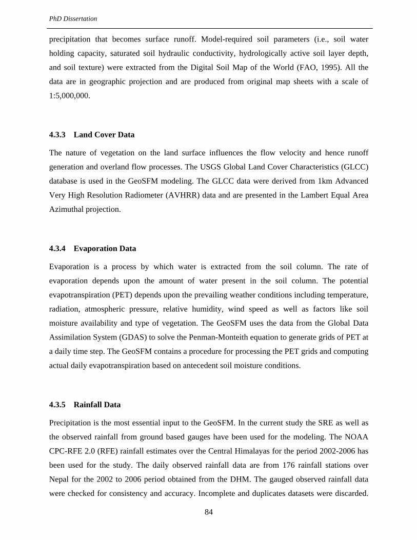
PhD Dissertation
84
precipitation that becomes surface runoff. Model-required soil parameters (i.e., soil water
holding capacity, saturated soil hydraulic conductivity, hydrologically active soil layer depth,
and soil texture) were extracted from the Digital Soil Map of the World (FAO, 1995). All the
data are in geographic projection and are produced from original map sheets with a scale of
1:5,000,000.
4.3.3 Land Cover Data
The nature of vegetation on the land surface influences the flow velocity and hence runoff
generation and overland flow processes. The USGS Global Land Cover Characteristics (GLCC)
database is used in the GeoSFM modeling. The GLCC data were derived from 1km Advanced
Very High Resolution Radiometer (AVHRR) data and are presented in the Lambert Equal Area
Azimuthal projection.
4.3.4 Evaporation Data
Evaporation is a process by which water is extracted from the soil column. The rate of
evaporation depends upon the amount of water present in the soil column. The potential
evapotranspiration (PET) depends upon the prevailing weather conditions including temperature,
radiation, atmospheric pressure, relative humidity, wind speed as well as factors like soil
moisture availability and type of vegetation. The GeoSFM uses the data from the Global Data
Assimilation System (GDAS) to solve the Penman-Monteith equation to generate grids of PET at
a daily time step. The GeoSFM contains a procedure for processing the PET grids and computing
actual daily evapotranspiration based on antecedent soil moisture conditions.
4.3.5 Rainfall Data
Precipitation is the most essential input to the GeoSFM. In the current study the SRE as well as
the observed rainfall from ground based gauges have been used for the modeling. The NOAA
CPC-RFE 2.0 (RFE) rainfall estimates over the Central Himalayas for the period 2002-2006 has
been used for the study. The daily observed rainfall data are from 176 rainfall stations over
Nepal for the 2002 to 2006 period obtained from the DHM. The gauged observed rainfall data
were checked for consistency and accuracy. Incomplete and duplicates datasets were discarded.
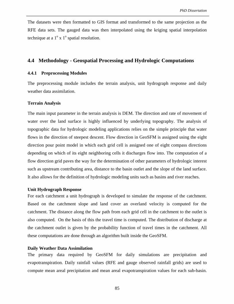
PhD Dissertation
85
The datasets were then formatted to GIS format and transformed to the same projection as the
RFE data sets. The gauged data was then interpolated using the kriging spatial interpolation
technique at a 1o x 1o spatial resolution.
4.4 Methodology - Geospatial Processing and Hydrologic Computations
4.4.1 Preprocessing Modules
The preprocessing module includes the terrain analysis, unit hydrograph response and daily
weather data assimilation.
Terrain Analysis
The main input parameter in the terrain analysis is DEM. The direction and rate of movement of
water over the land surface is highly influenced by underlying topography. The analysis of
topographic data for hydrologic modeling applications relies on the simple principle that water
flows in the direction of steepest descent. Flow direction in GeoSFM is assigned using the eight
direction pour point model in which each grid cell is assigned one of eight compass directions
depending on which of its eight neighboring cells it discharges flow into. The computation of a
flow direction grid paves the way for the determination of other parameters of hydrologic interest
such as upstream contributing area, distance to the basin outlet and the slope of the land surface.
It also allows for the definition of hydrologic modeling units such as basins and river reaches.
Unit Hydrograph Response For each catchment a unit hydrograph is developed to simulate the response of the catchment.
Based on the catchment slope and land cover an overland velocity is computed for the
catchment. The distance along the flow path from each grid cell in the catchment to the outlet is
also computed. On the basis of this the travel time is computed. The distribution of discharge at
the catchment outlet is given by the probability function of travel times in the catchment. All
these computations are done through an algorithm built inside the GeoSFM.
Daily Weather Data Assimilation The primary data required by GeoSFM for daily simulations are precipitation and
evapotranspiration. Daily rainfall values (RFE and gauge observed rainfall grids) are used to
compute mean areal precipitation and mean areal evapotranspiration values for each sub-basin.
PhD Dissertation
86
On the basis of antecedent soil moisture conditions and the data from the GDAS evaporation
time series are generated.
4.4.2 Hydrologic Simulation Modules
The hydrologic simulation modules include soil moisture accounting, channel flow routing and
computing spatial statistics.
Soil Moisture Accounting Soil moisture condition on a daily basis is computed for each catchment. The soil parameters of
each catchment are extracted from the DMSW produced by FAO and UNESCO. In the model
there are two soil moisture accounting routines: the single layer soil model and the two layer soil
model. Where there is limited data availability the single layer model is widely used which
however does not account for land cover within a catchment. In areas where finer resolution data
is available the two layer soil model is used which has a more complete representation of
subsurface processes by creating separate soil layers within which interflow and baseflow
processes occur.
Channel Flow Routing When runoff generated within a given catchment arrives at the catchment outlet, it enters the
river network and works its way downstream to the basin outlet. Within the GeoSFM model
there are three methods for routing, two linear methods namely pure translation and diffusion
analog, and one non-linear method, the Muskingum Cunge. For the current study the diffusion
analog routing method has been used given its simplicity and better generation of results
compared to other two routing methods.
Diffusion Analog Routing
The diffusion analog method is a linear transport routine. It is similar to the lag routing except
that it accounts for both flow advection (using a flow time or celerity) and attenuation (using a
flow dispersion coefficient). The diffusion analog equation is in fact the linear solution of the
Advection-dispersion equation (also known as the Navier-Stokes equation) for a plane
rectangular source (Maidment, 1993). Mathematically, the diffusion analog equation can be
expressed by using a series of equations as described below.
(1)

PhD Dissertation
87
(2)
where Q is discharge at location x along the channel, A is channel cross-sectional area, q is the
lateral inflow, and the friction slope, Sf can be parameterized using Mannings’s equation
| |. (3)
| | (4)
where C is the Chezy’s coefficient.
For a rectangular channel the continuity and momentum equation can be written as
(5)
where D is the Diffusion coefficient and is estimated as
(6)
where v is an advective velocity estimated as
(7)
where Kc is the conveyance given as
√ (8)

PhD Dissertation
88
And finally the Diffusion equation is given by
. . expD
(9)
where x is the location for forecast point downstream or the length of the river reach in m.
D is the dispersion coefficient in m2/s
V is the advection velocity or the flow celerity in m/s
x is the length of the river reach in m
to is the time of the input event in seconds
t is the present time in seconds
is the numerical constant Pi and has a value of 3.14159
Q(t) is the discharge at the downstream end of the river reach
I(to) is the inflow at the upstream end of the river reach.
4.4.3 Post Processing Modules
The post processing module in the GeoSFM includes calibration, sensitivity, flow statistics and
flow status maps.
Sensitivity Analysis Sensitivity analysis (SA) is an important step towards model calibration. Sensitivity analysis has
a dual purpose of testing which sensitive parameters should be used for calibration as well as
analyzing feasible parameter ranges. Sensitivity analysis allows us to see if there is a change in
model results when the parameter values are changed. The SA result can be used to test the
model structure, if parameters assumed to have a strong impact on model results do not show any
sensitivity, the model structure should be reassessed.
Model Calibration The purpose of calibration is to adjust the model parameters so that the model closely matches
the real system. Although many GeoSFM model parameters are derived from spatially

PhD Dissertation
89
distributed observed data, uncertainties in parameter adjustment to differences in scale,
uncertainty in deriving the parameter values from observed data, and uncertainties in the
structure of the model require that parameters be adjusted to overcome what we do not know,
and cannot measure about the watershed. These issues apply to all hydrologic models. Built
within the GeoSFM is a parameter calibration module which includes a sensitivity analysis
routine and a model calibration routine. The sensitivity analysis determines which parameters are
to be adjusted during the calibration process. There are twenty parameters in the model (eg. soil
water holding capacity, hydraulic conductivity, soil depth, curve number, river loss coefficients,
pan coefficient, etc) and the sensitivity analysis thus significantly reduces the time taken to
calibrate the model. The model calibration routine is an automatic calibration process using the
Multiobjective Shuffled Complex Evolution Metropolis (MOSCEM) Algorithm. It is an
automatic optimization process which finds the optimum parameters to minimize the difference
between the model simulated output and the observed output values. There are several objective
functions available within the model for example RMSE, NSCE among others to carry out the
optimization of the parameters. Manual calibration of the model can also be conducted by
adjusting the parameters identified during the sensitivity analysis by trial and error process.
Flow Statistics At the end of a simulation run, flow statistics provides a summary of the results. GeoSFM
includes a tool for computing a variety of flow statistics including the maximum, minimum,
mean, standard deviation, median, 25th, 33rd, 66th, and 75th percentile flows for each basin. The
results of the flow statistics computations are stored in the form of tables which are linked to the
basin data layer.
Flow Status Maps
Flow Percentile Map
Visual maps are considerably easier to interpret than tabular time series data particularly when
dealing with large river basins. GeoSFM contains a tool for displaying the results of simulations
for any given date in a visual map. The stream flow values on a user-selected date are presented
in the form of indices which present the values in the context of predefined criteria. The default
criterion for differentiating between low and normal flow is the 33rd percentile flow for the
analysis period, while the 66th percentile flow is the minimum threshold separating normal flow
and high flows. However, the user can define other criteria such as return period flow or

PhD Dissertation
90
predetermined drought and flood warning levels for the classification of flows. Each basin is
assigned a flow status index of 1, 2 or 3 to signify the respective low, normal and high flow
conditions. A color-coded map is then produced showing the flow status of each basin for the
select day.
Flow Hydrographs
GeoSFM contains a graphing tool for plotting hydrographs at the completion of a simulation run.
The tool can be activated from either a program menu or the tool menu bar. The user can then
visually select the basin for which a hydrograph is required by clicking on the basin in the visual
interface. The program automatically matches the spatial information with the time series and
produces a hydrograph. The flexibility of this tool is limited by ArcView’s rather limited
charting capabilities. The user is consequently encouraged to import the ASCII files resulting to
flow simulations into spreadsheet programs such as Microsoft’s Excel for more sophisticated
time series plotting capabilities.
4.5 Model Performance Indicators used for the Study
There is no single model performance indicator that determines the strengths and weakness of a
particular model. For determining the model performance it is desirable to adopt a variety of
different statistics and tests and decisions be made on the basis of these tests (Weeks and
Hebbert, 1980). A variety of tests, including those described by Aitken (1973), Nash and
Sutcliffe (1970) were utilized in this study to evaluate the performance of the GeoSFM model. In
the model performance indicators that are described below Qo and Qs are observed and simulated
discharge, and are the mean of the observed and simulated discharge. N is the number of
samples.
4.5.1 Correlation Coefficient
The standard correlation coefficient is one of the indicators used to describe the agreement
between the observed and simulated flows. It is defined as
∑ ∑ ∑
(10)

PhD Dissertation
91
4.5.2 Nash Sutcliff Coefficient of Efficiency (NSCE)
The Nash-Sutcliffe Coefficient of Efficiency (NSCE) (Nash and Sutcliffe, 1970) is commonly
used to evaluate the fit of the predicted hydrograph with observed. The perfect value is 1. It is
calculated as:
[ ][ ]
⎥⎥⎥⎥
⎦
⎤
⎢⎢⎢⎢
⎣
⎡
∑ −
∑ −−=
=
=N
ioo
N
ios
QQNSCE
1
12
2
1
(11)
4.5.3 Bias
The bias is the difference between the simulated and observed discharge and is defined as
∑ (12)
4.5.4 Root Mean Square Error (RMSE)
The RMSE provides greater emphasis on larger error and is defined as
∑ (13)
4.5.5 Peak Flow Error
The accuracy of flood prediction is evaluated using the peak flow error which is expressed in
percentage. The peak flow error is defined as
∑ 100 (14)
where Ep is the peak flow error in %, Qps is the peak simulated discharge, Qpo is the peak
observed discharge and n is the number of peaks above a defined threshold corresponding to the
discharge of the warning water level of the river.

PhD Disse
4.6 Ge
The loca
river syst
three clim
zone betw
(Jha, 200
part of th
areas inc
upper par
forest, w
predomin
accounts
ertation
eoSFM M
ation and gen
tem of the B
matic zones:
ween 1000
02; Dulal et
he watershed
clude Kathm
rt of the wat
with the great
nantly cultiv
for about 38
odel of the
neral charac
Bagmati is i
: the subtrop
and 2000 m
al., 2006).
d is mainly
mandu, Bhakt
tershed. The
ter part cove
vated. Forest
8%. The dom
Figur
e Bagmati
cteristics of
llustrated in
pical subhum
m and the co
The average
cultivated w
tapur and Pa
middle part
ered with fo
t accounts fo
minant soil ty
re 4.3 River
92
i Basin
the catchme
n Figure 4.3.
mid zone bel
ol temperate
e rainfall of
with limited
atan of the K
t of the wate
rest. The low
or 58% of th
ype is loamy
system of th
ent has been
. The Bagma
low 1000 m
e humid zon
the basin is
forest and a
Kathmandu V
ershed is a co
wer part of t
he total basi
y soil.
he Bagmati B
n provided i
ati basin can
m, the warm
ne between 2
s about 1800
a few other
Valley, whic
ombination o
the catchme
in area, whil
Basin
in chapter 3
n be divided
temperate h
2000 and 30
0 mm. The u
land uses. U
ch lies withi
of cultivation
ent in the Te
le cultivated
. The
d into
humid
000m
upper
Urban
in the
n and
erai is
d land

4.6.1 D
For the c
digital e
capacity,
texture) w
Land Co
Lambert
data and
rainfall d
including
Pandhera
hydrolog
Figure 4.
Figu
The Geo
Data Parame
current study
elevation mo
, saturated s
were extract
over Charact
Azimuthal E
streamflow
data covered
g 14 stations
a Dovan fro
gical and me
.4.
ure 4.4 Loca
SFM model
eterization a
y, the Bagm
odel Hydro
soil hydrauli
ted from the
teristics (GL
Equal Area p
gauge data
the period 2
s within the
om 2002 to
eteorologica
ation of rainf
was applied
and Analys
mati Basin bo
1k. Model-r
ic conductiv
Digital Soil
LCC) databas
projection is
were provid
2002 through
e Bagmati B
2004 was
al stations in
fall and disch
d for three di
93
is
oundary was
required so
vity, hydrolo
l Map of the
se derived f
s used in the
ded by DHM
h 2004 and w
Basin. The da
also availab
n the Bagm
harge gauginvicinity
ifferent case
s delineated
il paramete
ogically activ
e World (FA
from 1km A
GeoSFM m
M of the Gov
was provided
aily discharg
ble for the
ati Basin an
ng stations in
s:
P
and clipped
ers (i.e., soi
ve soil laye
AO, 1995). T
AVHRR data
modelling. Th
vernment of
d for 176 sta
ge data of B
study. The
nd its vicini
n the Bagma
Pandhera Dova
PhD Disser
d from this g
il water ho
r depth, and
The USGS G
a projected i
he rainfall st
Nepal. The
ations over N
Bagmati Bas
locations o
ity are show
ati Basin and
an
rtation
global
olding
d soil
Global
in the
tation
daily
Nepal
sin at
of the
wn in
d its

PhD Dissertation
94
1. Case 1: With the gauged observed rainfall over a peak flooding period. The run was for
38 days period, July 1 – August 7, 2002. The run was during monsoon caused peak flood
period.
2. Case 2: With the RFE data over the same 38 days period
3. Case 3: With the RFE for 2002 to 2004 period.
4.6.2 Results and Discussion
Simulated streamflow with gauge observed rainfall of July 2002
The simulated hydrograph over the 38-day period in 2002 (July 1 to August 7) using the gauge
observed rainfall compares well with the observed flows (Figure 4.5). The magnitude of the daily
simulated flow and timing matched well the observed flow magnitude and timing during the high
flow period (Figure 4.5). The high NSCE (0.91) and correlation (0.95) indicate a good fit
between observed and simulated flows. The scatter plot of the simulated and observed flows is
presented in Figure 4.6. Our findings of good correlation and performance of the model with
gauged observed rainfall data is consistent with the findings of previous studies (Hapuarachchi et
al., 2007; Kafle et al., 2006; Sharma et al., 2007; Artan et al., 2007b). The excellent match at the
peaks between simulated and observed flows indicates that the model can be used effectively for
flood forecasting.
Figure 4.5 Observed and simulated daily flows at Panheradovan, the daily flows were simulated using gauge observed rainfall data (July 1 – August 7, 2002)

PhD Dissertation
95
Figure 4.6 Scatter Plot of daily Observed and Simulated Discharge (July 1 – August 7, 2002)
Results of Model with the RFE Rainfall of July 2002
For the same period from July 1 to August 7, 2002 without readjusting the GeoSFM parameters
the model was driven with the RFE data. The comparison of observed and simulated flows is
presented in Figure 4.7. We find that with the RFE data the GeoSFM underestimates the peak
flow compared with observed gauge rainfall. We can also observe that there is a shift in the
timing and the sharpness of the peak. The NSCE of 0.15 and correlation of 0.50 were achieved.
The scatter plot of the simulated and observed flows is presented in Figure 4.8. Hapuarachchi et
al. (2007) explored the applicability of satellite-based precipitation data for near real-time flood
forecasting considering satellite based products from CMORPH, TRMM 3B42RT and GSMaP.
A grid based distributed hydrological model (BTOP) was used to generate river flow of Yoshino
basin in Japan. With gauged precipitation the NSCE was 0.84 while with CMORPH, 3B42RT
and GSMaP were 0.06, 0.52 and -0.06 respectively. The findings of the current study are
consistent with Hapuarachchi (2007) with the gauged precipitation performing well compared to
the RFE. Artan et al. (2007b) found poor agreement between the observed and RFE simulated
flows for the Se Done basin, a tributary of the Mekong River in Laos when the model was
calibrated with rain gauge measured rainfall data. Similarly when applied to the Nyando basin in
Kenya, tributary to Lake Victoria, the model with the RFE data considerably loses predictive
skills in contrasts to if gauged observed rainfall are used. The Se Done and Nyando are midsize
basins (6000 and 2600 km2) as the Bagmati Basin. The poor results for simulated flows with
R2 = 0.9104
0
1000
2000
3000
4000
5000
6000
0 1000 2000 3000 4000 5000 6000
Observed discharge (m3/sec)
Sim
ulat
ed D
isch
arge
(m3 /s
ec)

PhD Dissertation
96
RFE suggest that the RFE is not a suitable rainfall data for input to hydrologic models for basin
with the size of the Bagmati Basin.
Figure 4.7 Comparison of observed and simulated daily flows at Pandheradovan using gauge
observed rainfall and RFE data as an input rainfall (July 1 – August 7, 2002)
Figure 4.8 Scatter plot of observed and simulated discharge when the GeoSFM was driven
with RFE (July 1 – August 7, 2002)
Streamflow Simulation using RFE for 2002, 2003 and 2004
As poor agreement was found between the gauge observed and RFE simulated flows for
Bagmati Basin when the model was calibrated with rain gauge measured rainfall data further
analysis was done to recalibrate the GeoSFM with RFE. As three years of daily discharge
data was available the period 2002 to 2003 was taken as the calibration period and 2004 for
validation. Parameters were adjusted to provide the best simulated results using the RFE. The
calibration was considered to be complete when no further improvement or very little change
0
1000
2000
3000
4000
5000
6000
0 5 10 15 20 25 30 35 40Days
Dis
char
ge (m
3 /sec
)
Observed Simulated (gauge) Simulated (RFE)
R2 = 0.2543
0500
10001500200025003000350040004500
0 1000 2000 3000 4000 5000 6000
Observed discharge (m3/sec)
Sim
ulat
ed D
isch
arge
(m3 /s
ec)

PhD Dissertation
97
was observed in the predicted flows even when varying the parameters. This involved
successive changes in the parameter values identified as sensitive during the sensitivity
analysis until the best fit was obtained. Comparison of observed and simulated hydrographs
from the model is summarized in Figure 4.9. The year 2002 and 2003 the agreement between
the observed and simulated flows was marginal. The NSCE was 0.23 with a correlation of
0.59.
Figure 4.9 Observed and simulated streamflows using RFE from 2002 to 2004 (calibration)
Using the same parameters from the calibration period the GeoSFM was run for 2004 using
2004 RFE. The predicted peak flows in 2004 were extremely low compared to the observed
flows as presented in Figure 4.10. The performance of the validation period was not satisfactory.
When the model is driven with an RFE it under predicted considerably the flows. When the
model was calibrated with the RFE soil water holding capacity (SWHC) value becomes
significantly lower than the at prior estimated values at around 100 mm per 1 meter of soil.
Figure 4.11 shows a box plots of the SWHC that were estimated when the two rainfall data were
use. Where the SWHC estimated from the calibration of the gage data is reasonable of what
could be expected for the dominant soil types present in the basin (silty clay loam and clay loam
soil types).
The poor performance of the results could be due to a number of reasons. Firstly, the
calibration period i.e. 2002 to 2003 may not have been appropriate or long enough. Secondly, the
0
1000
2000
3000
4000
5000
6000
0 100 200 300 400 500 600 700
Days
Dis
char
ge (m
3 /sec
)
Observed Simulated (RFE)

PhD Dissertation
98
quality of data/RFE is questionable at best. Thirdly, the 2004 RFE must be significantly
underestimating rainfall resulting in an amplification of error into a large flow underestimation.
Figure 4.10 Observed and simulated flows for 2002-2005
In a study conducted by Hughes et al. (2006) the results of the validation period using the
satellite rainfall data were poorer compared to the calibration period in the Okavango river. The
current results also indicate similar findings.
Figure 4.11 Average soil water holding capacity of the 21 sub-basins modelling units when the GeoSFM (a) is calibrated with satellite-based rainfall fields, and (b) when the model is
calibrated with rain
In the past several studies have been done to assess the runoff of the Bagmati Basin using
various rainfall-runoff models and satellite data. Kafle (2007) used the HEC-HMS hydrologic
model with TRMM and rain gauge data to simulate flows of the Bagmati. Sharma et al. (2007)
has made comparison with TRMM 3B42RT data and rain gauge data and applied the results to
predict floods in the Bagmati Basin. He observed that the TRMM data has underestimated the
0
1000
2000
3000
4000
5000
6000
0 200 400 600 800 1000 1200
Days
Dis
char
ge (m
3 /sec
)
Observed Calibrated (RFE) Validated (RFE)
60
80
100
120
140
Gag
e.So
ilWH
C..m
m.
8
10
12
14
16
SBR
.Soi
lwhc
..mm
.

PhD Dissertation
99
monsoon rainfall peaks. The findings of these studies in the past are in agreement with the
current findings where with the rain gauge data the model predicted the peak discharge fairly
accurately while the satellite data underestimated the discharge significantly as was observed
from the one month simulation in 2002. This indicates that the accuracy of the RFE has to be
improved further to realistically predict the floods of the basin and become useable product for
an operational flood forecasting system for the Bagmati River.
4.7 GeoSFM Model of the Narayani Basin
The location and general physiographic description of the Narayani Basin has been presented in
the previous chapter. The location of the rainfall stations in and within the vicinity of the
Narayani Basin is shown in Figure 4.12.
Figure 4.12. Location of the rainfall stations within and in the vicinity of the Narayani Basin
4.7.1 Data Parameterization and Analysis
The Narayani Basin boundary was delineated and clipped from this global digital elevation
model Hydro1k. Similar to the Bagmati Basin the model-required soil parameters (i.e., soil water
Devghat Hydrological station

PhD Dissertation
100
holding capacity, saturated soil hydraulic conductivity, hydrologically active soil layer depth,
and soil texture) were extracted from the Digital Soil Map of the World (FAO, 1995). The USGS
Global Land Cover Characteristics (GLCC) database derived from 1km AVHRR data projected
in the Lambert Azimuthal Equal Area projection is used in the GeoSFM modelling. The rainfall
station data and streamflow gauge data were provided by DHM of the Government of Nepal. The
daily rainfall data covered the period 2002 through 2006 and was provided for 176 stations over
Nepal including 45 stations within the Narayani Basin. The daily discharge data of Narayani
River at Devghat from 2002 to 2006 was also made available by DHM for the study. The
locations of the hydrological and meteorological stations in the Narayani Basin and its vicinity
are shown in Figure 4.12.
This focus of this study is the four months of the monsoon June, July, August, and September
when floods occur in the basin. The gridded gauge observed rainfall data for the monsoons of
2003 and 2004 were used in the GeoSFM to predict floods. Daily observed river discharge data
from the 2003 monsoon were used for GeoSFM model calibration and data from 2004 for
validation. The reliability of the RFE rainfall estimates for flood prediction was evaluated using
the 2003 monsoon data.
4.7.2 Results and Discussion
Calibration and validation of the GeoSFM with gauge observed rainfall
The calibration of the GeoSFM for the Narayani Basin was performed using daily gauge
observed rainfall data from June to September 2003. A high NSCE (0.84) and a highly
significant correlation (0.94) indicate a relatively robust calibration with a good fit between
observed and simulated discharge. The RMSE was 754.3 with an average discharge error of -3 %
over a threshold of 7500 m3/sec. The threshold discharge of 7500 m3/sec corresponds to the
warning level of 6.8 m at the Devghat hydrological station. The average peak discharge error
was -7.6% for the three peaks. Overall, the magnitude and timing of the simulated peak
discharge matched well with the observed. Figure 4.13 presents the comparison and scatter plot
of the simulated and observed discharge. In the Bagmati Basin about ten times smaller than
the Narayani Basin a similar high NSCE of 0.91 and r of 0.95 were obtained (Shrestha et al.,
2008). The GeoSFM therefore predicts the flows accurately when gauge observed data are
applied and calibrated in small and large basins indicating reliable application to flood
forecasting with improved quality of rainfall estimates.
PhD Dissertation
101
Figure 4.13 Comparison and scatter plot of observed and simulated discharge at Devghat using 2003 monsoon gauge observed rainfall (June to September)
The validation of the GeoSFM was performed using rainfall data from June to September of
2004. An NSCE of 0.77, RMSE of 697.1 and a highly significant correlation coefficient of 0.94
were achieved. The peak flow error was about -3%. All flood peaks during this year was lower
than the threshold discharge corresponding to the warning level so no discharge error above the
threshold was computed. Figure 4.14 presents the comparison of simulated and observed
hydrographs and scatter plot indicating a fairly good fit.
Figure 4.14 Comparison and scatter plot of daily observed and simulated discharge at Devghat using 2004 monsoon gauge observed rainfall (June to September)
Flood Prediction using CPC_RFE2.0 (RFE) rainfall estimates
A simulation run of the GeoSFM model forced with the RFE for the period June to September
2003 was obtained. The model parameters obtained from the calibration of the GeoSFM with the
gauge observed rainfall data were not readjusted. The hydrograph simulated with the RFE
0
20
40
60
80
100
120
140
160
1800
2000
4000
6000
8000
10000
12000
14000
16000
152 162 172 182 192 202 212 222 232 242 252 262 272
Rai
nfal
l (m
m)
Dis
char
ge (m
3 /sec
)
Time (Days)Gauge Rain Observed Discharge Simulated Discharge (Gauge)
y = 0.8298x + 802.64R² = 0.8839
0
2000
4000
6000
8000
10000
12000
0 2000 4000 6000 8000 10000 12000
Obs
erve
d di
scha
rge (
m3 /s
ec)
Simulated discharge (m3/sec)
0
10
20
30
40
50
60
70
800
2000
4000
6000
8000
10000
12000
152 162 172 182 192 202 212 222 232 242 252 262 272
Rai
nfal
l (m
m)
Dis
char
ge (m
3 /sec
)
Time (Days)Gauge Rain Observed Discharge Simulated Discharge (Gauge)
y = 0.7624x + 1061.8R² = 0.8797
0
1000
2000
3000
4000
5000
6000
7000
8000
0 2000 4000 6000 8000
Obs
erve
d di
scha
rge (
m3 /s
ec)
Simulated discharge (m3/sec)

PhD Dissertation
102
considerably underestimated the peak flows when compared with the hydrograph simulated with
gauge observed rainfall (Figure 4.15). Also, the fact that RFE simulated streamflow missed some
of the peaks, points to the presence of random errors in the RFE data. A low NSCE of -1.17, a
high RMSE of 2805 and correlation coefficient of 0.69 were achieved indicating a significant
underestimation of flow but still with a relatively significant correlation. The average peak
discharge error using RFE was -53%. The average error above the threshold discharge
corresponding to the warning level was -61%. Figure 6 shows the scatter plot of the simulated
and observed flows (R2 = 0.47) with significant underestimation of flows. In the Bagmati Basin
(which is about ten times smaller than the Narayani), RFE simulated hydrographs showed an
underestimation of flows with a NSCE of 0.15 and a correlation of 0.50 (Shrestha et al., 2008).
The increased correlation obtained in the Narayani Basin simulation suggests better performance
of GeoSFM in larger basins. But, the reduced NSCE, increased RMSE and peak discharge error
compared to the Bagmati indicates deterioration in flood prediction using the RFE rainfall
estimates in the Narayani Basin where the terrain is complex with a large proportion of basin
area in the high mountains with greater influence of orography.
Figure 4.15 Comparison and scatter plot of daily observed and simulated discharge at Devghat using gauge observed rainfall and RFE data as input rainfall (June to September
2003)
Therefore, the poor skills of the GeoSFM hydrological model to predict the magnitude of the
floods when using the RFE, compared to when using gauge observed rainfall, suggest that the
increased uncertainty of flood prediction is a result of inaccurate satellite-based rainfall inputs
rather than the modelling of the hydrological processes, thus, making imperative the de-biasing
or improvement of the SRE prior to use in predicting floods.
0204060801001201401601802000
2000
4000
6000
8000
10000
12000
14000
16000
152 162 172 182 192 202 212 222 232 242 252 262 272
Rai
nfal
l ( m
m)
Dis
char
ge (m
3/se
c)
Time (Days)
Gauge Rain Observed Discharge Simulated Discharge (Gauge) Simulated Discharge (RFE)
y = 1.1474x + 2251.2R² = 0.4709
0
2000
4000
6000
8000
10000
12000
0 2000 4000 6000 8000 10000 12000
Obs
erve
d di
scha
rge (
m3 /s
ec)
Simulated discharge (m3/sec)

PhD Dissertation
103
Flood Prediction using CPC_RFE2.0 (RFE) rainfall estimates calibrated model
A simulation run of the GeoSFM model forced with the RFE rainfall estimates for the period
June to September 2003 was obtained. In this simulation the model was calibrated using the RFE
estimates instead of using the parameters obtained from the calibration of the GeoSFM with the
gauge observed rainfall data. By recalibrating the model with RFE a slight improvement in the
performance of the model is seen though the hydrograph simulated with the recalibration still
underestimates the peak flows when compared with the hydrograph simulated with gauge
observed rainfall (Figure 4.16). The NSCE increases from -1.17 to -0.36 and correlation
coefficient from 0.69 to 0.76 while the RMSE decreases from 2805 to 2174. The average error
above the threshold discharge corresponding to the warning level was decreases to -41% from -
61%. Figure 4.16 shows the scatter plot of the simulated and observed flows (R2 = 0.58) with
significant underestimation of flows. The improvement in the results indicates that the model has
to be recalibrated with the RFE rainfall estimates for discharge prediction with RFE. However,
even with improvement the RMSE and peak flow error are large with the recalibrated model
suggesting that the RFE has to be bias-corrected before further use in discharge prediction.
Figure 4.16 Hydrograph and scatter plot of daily observed and simulated discharge at Devghat with RFE calibrated model from June to September 2003
4.8 Summary
The GeoSFM, a semi-distributed physically based hydrological model developed by the USGS
was used to simulate the discharge using remotely sensed and widely available global datasets
for the Bagmati and Narayani Basins in Nepal. Bagmati has a catchment area of 2800 km2 at the
Padheradovan gauging station while the Narayani is about 32,000 km2 at Devgaht gauging
station. The interpolated gauge observed rainfall data and SRE from NOAA at 0.1 x 0.1 degree
0
2000
4000
6000
8000
10000
12000
152 162 172 182 192 202 212 222 232 242 252 262 272
Dis
char
ge (m
3 /sec
)
Time (Days)
Observed Discharge Simulated Discharge (RFE)
y = 0.785x + 2199.5R² = 0.5781
0
2000
4000
6000
8000
10000
12000
0 2000 4000 6000 8000 10000 12000
Obs
erve
d di
scha
rge (
m3 /s
ec)
Simulated discharge (m3/sec)

PhD Dissertation
104
spatial resolution on a daily basis were used to simulate the flows. The GeoSFM model was
calibrated using the gauge observed monsoon data from June to September 2003 for the
Narayani Basin and for from 1st July to 7th August 2002 for the Bagmati Basin. Satisfactory
validation of the model was obtained using the gauge observed monsoon data. The same
parameters obtained during the calibration were used for the validation of the model which
showed good agreement with the observed. Thus we can infer that GeoSFM predicts the flows
accurately when observed rain gauge data have been applied and calibrated indicating reliable
application to flood forecasting with improved quality of rainfall estimates.
Discharge was then simulated with RFE using the calibrated parameters from the 2002
and 2003 monsoon data for Bagmati and Narayani respectively, which showed
underestimation of flood prediction. The hydrograph simulated with the RFE considerably
underestimated the peak flow when compared with the hydrograph simulated with gauge
observed rainfall. The accuracy in RFE estimates was assessed by comparing the gauge
observed and estimated rainfall in those grids with one or more stations. The RFE captures the
rainfall spatial trends well, but underestimates the amount on average by more than 50 per cent.
As the magnitude of the rainfall is much lower in the RFE compared to the gauged observed
rainfall there is underestimation of simulated flows when the RFE dataset is used to force the
hydrologic model. The underestimation of simulated flows when using the RFE data is an
agreement with results from previous research on the matter. It is thus difficult to predict the
floods quantitatively using current satellite based data. We can only give an indication of
probability of occurrence. This suggests that remotely sensed rainfall estimates needed to be
adjusted prior to use for flood prediction.
References
Aitken, A.P. (1973) Assessing Systematic Errors in Rainfall-Runoff Models. J. Hydrol., Vol. 20.
121-136.
Artan, G.A.; Asante, K.O.; Smith, J.L.; Pervez, S.; Entenmann, D.; Verdin, J.P.; Rowland, J.
(2007b) Users manual for the Geospatial Stream Flow Model (GeoSFM). US Geological
Survey Open-File Report 2007-1440, p.194. Reston, Virginia.

PhD Dissertation
105
Artan, G.A.; Gadain, H.; Smith, J.L.; Asante, K.; Bandaragoda, C.J.; Verdin, J.P. (2007a)
Adequacy of satellite derived rainfall data for streamflow modelling. Nat. Hazards, 43, 167-
185.
Asante, K.O.; Artan, G.A.; Pervez, S.; Bandaragoda, C.; Verdin, J.P. (2007b) Technical manual
for the Geospatial Stream Flow Model (GeoSFM). US Geological Survey Open-File Report
2007–1441, p. 99. Reston, Virginia.
Asante, K.O.; Macauacua, R.D.; Artan, G.A.; Lietzow, R.W.; Verdin, J.W. (2007a) Developing a
flood monitoring system from remotely sensed data for the Limpopo Basin. IEEE Trans.
Geosci. Remote Sens. 45(6), 1709–1714.
Bhusal, J.N.; Bhattarai, K.P. (2002) Lessons from the extreme floods in south central Nepal in
1993. International Basin of Network Organization’s (INBO) General Assembly, Quebec
City.
Chalise, S.R., Shrestha, M.L., Thapa, K.B., Shrestha, K.B., Bajracharya, B. (1996) Climatic and
hydrological Atlas of Nepal. Kathmandu: ICIMOD
Drayton, R.S.; Wilde, B.M.; Harris, J.H.K. (1992) Geographical information system approach to
distributed modelling, in: Beven, K.J., Moore, I.D. (Eds.), Terrain analysis and distributed
modelling in hydrology, John Wiley and Sons, pp. 253-368, West Sussex.
Harris, A.; Hossain, F. 2008. Investigating the optimal configuration of conceptual hydrologic
models for satellite-rainfall-based flood prediction. IEEE Geosci. Remote Sensing, 5(3), 532-
536.
Harris, A.; Rahman, S.; Hossain, F.; Yarborough, L.; Bagtzoglou, A.C.; Easson, G. (2007)
Satellite-based flood modelling using TRMM-based rainfall products. Sensors, 7, 3416–
3427.
Hong, Y.; Adler, R.F.; Negri, A.; Huffman, G.J. (2007) Flood and landslide applications of near
real-time satellite rainfall estimation. Nat. Hazards, 43, 285–294.
Hughes, D.A. (2006) Comparison of satellite rainfall data with observations from gauging station
networks. J. Hydrol., 327, 399–410.
Maidment, D.R. (1993) Handbook of Hydrology. McGraw Hill, New York, San Francisco.

PhD Dissertation
106
Moore, R.J.; Bell, V.A. (2001) Comparison of rainfall-runoff models for flood forecasting. Part
1: Literature review of models. Bristol, UK, Environment Agency, 94pp. (R&D Technical
Report W241, CEH Project Number: C00260)
Nash, J.E.; Sutcliffe J.V. (1970) River flow forecasting through conceptual models: Part 1-A
discussion on Principles. J. Hydrol., 10, 282–290.
Nash, J.E.; Sutcliffe J.V. (1970) River flow forecasting through conceptual models: Part 1-A
discussion on Principles. J. Hydrol., 10, 282–290.
Sharma, C.K. (1977) River systems of Nepal. Sangeeta Sharma, p. 214. Kathmandu.
Shrestha, M.S., Takara, K., Kubota, T., Bajracharya, S. (2011) Verification of GSMaP rainfall
estimates over the Central Himalayas. Annual Journal of Hydraulic Engineering, JSCE, Vol.
55 (to be published).
Shrestha, M.S.; Artan, G.A.; Bajracharya, S.R.; Sharma, R.R. (2008) Applying satellite based
rainfall estimates for streamflow modelling in the Bagmati Basin, Nepal. J. Flood Risk
Management, 1, 89–99.
Shrestha, M.S.; Bajracharya, S.R.; Mool. P. (2008) Satellite rainfall estimation in the Hindu
Kush-Himalayan region. Kathmandu: ICIMOD
Weeks, W.D.; Hebbert, R.H.B. (1980) A comparison of Rainfall-Runoff Models. Nordic
Hydrology., 11. pp 7-24.
Wilk, J.; Kniveton, D.; Andersson, L.; Layberry, R.; Todd, M.S.; Hughes, D.; Ringrose, S.;
Vanderpost, C. (2006) Estimating rainfall and water balance over the Okavango River Basin
for hydrological applications. J. Hydrol., 331, 18–29.
Wilks, D.S. ( 2006) Statistical methods in the atmospheric sciences, 2nd ed. Elsevier Academic
Press, Burlington. MA. p. 627.
Wilmott, C.J. (1982) Some comments on the evaluation of model performance. Bull. Amer.
Meteorol. Soc., 88, 1309–1313.
Wilmott, C.J.; Ackleson, S.G.; Davis, R.E.; Feddema, J.J.; Klink, K.M.; Legates. D.R.;
O’Donnell, J.; Rowe, C.M. (1985) Statistics for the evaluation and comparison of models. J.
Geophys. Res., 90 (C5), 8995–9005.
Xie, P.; Arkin, P.A. (1996) Analyses of global monthly precipitation using gauge observations,
satellite estimates and numerical model predictions. J. Clim., 9, 840–858.

PhD Dissertation
107
Xie, P.; Yarosh, Y.; Love, T.; Janowiak, J.; Arkin, P.A. (2002) A real-time daily precipitation
analysis over South Asia. Preprints, 16th Conf. of Hydro., Orlando, FL, Amer. Meteorol.
Soc.
Yilmaz, K.K.; Hogue, T.S.; Hsu, K.; Sorooshian, S.; Gupta, H.V.; Wagner, T. (2005)
Intercomparison of rain gauge, radar, and satellite-based precipitation estimates with
emphasis on hydrologic forecasting. J. Hydrometeorol., 6, 497–517.

PhD Dissertation
108
CHAPTER 5
5 BIAS-ADJUSTMENT OF SATELLITE-BASED RAINFALL
ESTIMATES
5.1 Introduction
From the previous chapter we have seen the discharge prediction in two river basins of Nepal
using the satellite-based rainfall estimates (SRE). The SREs are found to detect the occurrence of
rainfall and have a significantly good correlation with the gauge observed rainfall but failing to
adequately capture rainfall amounts. There is significant underestimation of rainfall leading to
lower predicted discharge suggesting the need for bias correction of SREs before it can be put
into operational use (Shrestha et al., 2008). The need for bias-adjustment of the global SREs for
application into water resources management and flood prediction have also been felt by Hughes
(2006), Harris et al. (2007).
The NOAA CPCP_RFE2.0 (RFE) rainfall estimates used in the present study is a satellite-
gauge merged rainfall estimate (Xie et al., 1996) available on a semi real time basis. Apart from
the RFE currently there are no other global satellite-based rainfall products with bias-corrected
rainfall estimates on a near real time basis. As explained in chapter 2 the TRMM 3B42_V6 is a
research product the rainfall estimates of which are adjusted by gauge data but not in near real
time. The TMPA was upgraded in early 2009 to include a climatological calibration to the post-
real-time research TMPA product but was still on testing phase.
The RFE algorithm uses available rain gauge information from the WMO GTS network to
remove bias from each satellite estimate component; hence the number of gauges used in each
daily product is very much related to the accuracy of the final product. Currently, the WMO
network of GTS gauges is relatively sparse for many of the HKH countries, thus essentially
forcing the RFE algorithm to rely primarily on satellite estimates in these locations. For example,
from Nepal only a few stations contribute to the GTS while none contribute from Bhutan. In
mountainous areas, there is both a lack of gauge information and a tendency for satellite rainfall
sensors to perform poorly, thus complicating the situation. Availability of larger number of
gauge observation at a local level provides an opportunity to merge these estimates at a local
level for improving the SREs.

PhD Dissertation
109
The research problem we address in this chapter is how can SREs be adjusted for better flood
prediction? Two approaches have been proposed to adjust the SREs. The first approach is a ratio
based bias-adjustment using various temporal scales of adjustment; monthly, seasonal and 7-day
moving average. The second approach is local tuning of SREs by ingesting the local rain gauge
data into the RFE algorithm. These two approaches have been used in correcting the SREs and
applied in hydrological modelling of the Narayani Basin in Nepal for the monsoon of 2003,
yielding encouraging results at a daily time scale. This chapter describes the bias correction
methods available in the literature, provides the procedure for bias correction developed for this
study and evaluates the procedure for flood prediction.
5.2 Bias-Adjustment
As has been stressed earlier the availability of rainfall data for hydrological modeling is limited
because of the sparse density of rain gauge data in various regions of the world particularly in
developing countries. Satellite based rainfall estimates which provide continuous spatial
variation of precipitation is one of the inputs that can drive a hydrological model however; the
accuracy of the estimates so far needs to be improved. The methods available for bias correction
of SREs are very few in the literature hence the methods in correcting the Regional Climate
Models (RCM) were reviewed as the methods are thought to be relevant for RFE. Regional
Climate Models are an important source of climate input for hydrological models. The RCM data
are used in hydrological model to address the impact of climate change on the hydrological
response of river basins. Though the scale of application is different from the current research the
bias-adjustment of the RCM has been reviewed having precipitation as the common
meteorological parameter to examine the impacts on the hydrological regime. Similar to the
problem of SREs in application into hydrological modeling, the RCM data is also faced with
inherent source of uncertainty coming from RCM’s inability to simulate present-day climate
conditions accurately. There are a number of studies that have applied bias correction to rainfall
estimates derived from Global Climate Models (GCM) (Terink et al., 2010; Hay et al., 2002;
Leander and Buishand, 2007; Piani et al., 2010). This section describes the methods for
correcting rainfall using gauge observed data.

PhD Dissertation
110
5.2.1 Gamma Transform for Bias-Adjustment
Hay et al. (2002) examined the use of RCM outputs for hydrologic modeling. The runoff using
RCM outputs were found to have large bias compared to the observed hydrograph. Bias
corrections were made on a monthly basis using a gamma transform. The Gamma transform
preserves the precipitation distribution in the observed and model values. This method requires
both the time series datasets of observed and model to be fit into a gamma distribution and
compute the cumulative probability in the distribution. The basic assumption is that both the
simulated and observed values can be approximated by using the same probability function. The
probability distribution function (PDF) of the satellite-based product is adjusted to the PDF of
the observed values, minimizing bias. It is assumed that the non-exceedance probability of the
observed and simulated is the same. As the bias correction is a magnitude correction of the
precipitation value Hay et al. (2002) found that the corrected precipitation did not contain the
day to day variability which was present in the observed data set. Piani et al. (2010) applied the
gamma transform method also known as the statistical bias correction to the daily precipitation in
regional climate models over Europe and obtained improvement in the model results. The
Gamma distribution with two parameters that is commonly used for rainfall analysis is given by
equation 1.
exp , 0, 0, 0 (1)
where α and β are shape and scaling parameters and x is the precipitation field.
For the current study this method was not adopted as only five years of overlap data between
the RFE and gauge observation was available which is not adequate to fit a gamma distribution
for obtaining bias corrections.
5.2.2 Power Transform for Bias-Adjustment
Leander and Buishand (2007) used a power transformation, which converts CV as well as the
mean of the rainfall estimates. This method of bias correction has been applied by Tirren et al.
(2010) in bias correcting RCM in the Rhine Basin. This is a non-linear correction of daily
precipitation and is given by equation 2.
= a (2)
where P is the precipitation amount and a and b are coefficients.

PhD Dissertation
111
Parameters a and b were determined for every five day period of the year. As a first step
parameter b was determined keeping the coefficient of variation (cv) of the corrected
precipitation matching the cv of the observed precipitation.
(3)
(4)
The parameter a is determined such that the mean of the transformed daily values correspond to
the observed values.
Applying this technique to the Rhine River Terink et al. (2010) found that the bias-adjusted
precipitation improved however, the RMSE of the daily precipitation differences between RMC
output and observed precipitation was not smaller for the corrected precipitation values. This
method was not adopted given the limitation of the number of years of data overlap available for
such a correction to be meaningful.
5.2.3 Ratio Based Bias-Adjustment
Ines and Hansen (2006) applied a simple concept of bias-adjustment by applying a multiplicative
shift to correct the bias of the mean monthly GCM rainfall. The concept is similar to the one
proposed in this research where a correction factor for various time periods is derived by
comparing the daily SREs with the gauge observed values. Though this procedure is said to
adjust only rainfall intensity to reproduce the long-term mean observed monthly rainfall, it is
seen to be adequate for flood prediction for capturing the peak discharges. The section below
describes the three ratio based bias-adjustments derived for this research.
As the RFE are available for the South Asia domain from 2002 and the gauge observed
rainfall data till 2006 there is an overlap of five years between the two data sets. Ideally for
obtaining bias correction a longer data series is required preferably more than 10 years.
However, with the five years of data from 2002 to 2006; the seasonal and monthly bias-
adjustments were derived comparing the RFE and gridded gauge observed rainfall data at grids
with one or more gauges. The bias-adjustment was derived using a two step procedure. Firstly,
the daily datasets were accumulated to monthly totals to obtain the ratio of the gridded gauge
observed rainfall to the RFE estimates at each grid with one or more rainfall stations. Then the
monthly values of ratio were averaged over all grids with one or more station. Similarly for a

PhD Dissertation
112
seasonal value the accumulated period was for JJAS instead of each month. The bias-adjustment
“Z” is given by equation 5.
(5)
where n is the number of grids with one or more rain gauges, Oi is the gauge observed rainfall, Pi
is the satellite-based rainfall and m is the number of years.
The bias corrections were derived on a seasonal, monthly and a 7 day moving average basis.
The method of bias-adjustment is schematically shown in Figure 5.1.
Figure 5.1 Methodology for bias correction
5.2.4 Improved Gauge-Satellite Merged Rainfall Estimates for Bias-Adjustment
The RFE is a daily satellite-gauge merged product which uses 3 SREs merged with GTS rain
gauge data. The satellite data sources are of data; AMSU-B; SSM/I and GPI cloud-top IR
temperature precipitation estimates. The three satellite estimates are first combined linearly
using daily, predetermined weighting coefficients, then are merged with station data to determine
the final rainfall. Although the RFE algorithm incorporates the available GTS data, much of the
time, data are not reported from the stations in near real time for various reasons. The number of
⎥⎦
⎤⎢⎣
⎡∑∑===
n
i i
im
i PO
nmZ
11
11
Gauge Observed rainfall Satellite‐based rainfall estimates
Accumulated daily rainfall estimates – 7‐day moving average, monthly and seasonal accumulation
Average ratio of observed accumulation to satellite‐based rainfall estimates for all grids
Average bias‐adjustment ratio for “n” number of years of data available
Bias corrected satellite‐based rainfall estimates
Discharge Prediction with Hydrological Model
Rainfall Data
Ratio of observed and satellite based rainfall estimates at each grid for 7‐day moving average, monthly and seasonal

PhD Dissertation
113
GTS stations that report on a timely and regular basis is limited affecting the accuracy of the
rainfall estimates. Therefore, at a country level, it is possible to access data from more gauges
than that available from the GTS. To increase the accuracy of temporal and spatial variability of
precipitation data, local rain gauge data may be added to the NOAA RFE algorithm and obtain
improved satellite-gauge merged rainfall products. The increase in accuracy of the rainfall
estimates depends upon the number of local rain gauges that can be added.
The RFE data can be downloaded from the ftp server using the NOAA algorithm available in
FORTRAN which runs in a windows version (NOAA 2009). For use with the Windows RFE
version, GTS, GPI, SSMI and AMSUB input files are available via anonymous ftp on a daily
basis. For the current study the three satellite inputs available during 2003 to 2006 were used
with modification to the GTS master file. The GTS master file was edited to incorporate the
additional rain gauge stations in the study area. As data from all over the Himalayan region was
available the master station file was modified to reflect additional 419 stations which include the
176 rainfall stations available from Nepal. Incorporation of a larger number of rainfall stations
from the whole HKH region prevents discontinuity of rainfall estimates at national borders.
Because no GTS data were found to report for the monsoon of 2003, all the quality checked
available gauge observed rainfall data were added to obtain a new GTS file for ingestion into the
algorithm. To de-bias satellite-based rainfall using gauge observed rainfall data, the algorithm
described by Xie and Arkin (1996) was used. Using the merging algorithm developed by Xie and
Arkin (1996), the SREs from SSM/I, AMSU-B, and GPI, and the new GTS datasets were
merged to come up with new gauge-satellite merged estimates for the 2003 monsoon over the
Narayani Basin (NOAA, 2009).
5.3 Rainfall-Runoff Simulation Using Bias-Adjusted Satellite-Based Rainfall
Estimates
5.3.1 Satellite-Based Rainfall Estimates with Bias-Adjustment
Three ratio based bias-adjustment factors were derived and applied to the RFE rainfall estimates.
The first bias-adjustment of 1.80 was derived for a season using a ratio between the total
volumes of gauge observed and RFE from June through September (JJAS) for 2002 to 2006
period, at those grids with one or more rainfall stations, as explained in the earlier section. Daily

PhD Dissertation
114
rainfall amounts from RFE and gauge observed rainfall were accumulated from June to
September to yield seasonal totals for each year from 2002 to 2006.
The second bias-adjustment was derived for each month instead of a season by comparing
the cumulative hyetographs on a monthly basis. Daily rainfall of the RFE and gauge observed
rainfall estimates were accumulated to monthly rainfall and ratios derived based on the monthly
accumulation for each year and averaged over a five year period from 2002 to 2006. The bias-
adjustments for June, July, August, and September were calculated to be 1.99, 2.0, 1.58, and
1.82, respectively.
With the aim to further improve the rainfall estimates for flood prediction purposes, a
moving bias-adjustment averaged over the previous seven-day period for the whole monsoon
season were derived. The seven-day period was chosen based on inspection of tests to represent
rainfall event duration. To further improve the flood prediction a new gauge-satellite merged
product was developed using the gauge observed data not included in the GTS and the Xie and
Arkin (1996) algorithm. Figure 5.2 provides the scatter plot of daily basin averaged SRE with
and without adjustments for the monsoon period for 2003. Figure 5.2 illustrates the improvement
in rainfall estimates by applying bias-adjustments compared to the unadjusted RFE. In the figure
we can see the unadjusted RFE underestimating the rainfall values while the best adjustment is
seen to be with improved RFE obtained from merging RFE with local rain gauge data.
0
10
20
30
40
50
60
70
80
90
0 10 20 30 40 50 60 70 80 90
Gau
ge o
bser
ved
rain
fall (
mm
)
Satellite-based rainfall estimates (mm)
RFE season month 7day improvedRFE

PhD Dissertation
115
Figure 5.2 Scatter plot of daily area averaged gauge observed rainfall and SRE with and without bias-adjustment for monsoon of 2003.
5.3.2 Rainfall Simulation with Bias-Adjusted Satellite-Based Rainfall Estimates
The GeoSFM hydrologic model was used to simulate the flows with bias-adjustment. The
parameters of the semi-distributed hydrological model are determined for each sub-basin derived
by dividing the basin into several sub-basins using the basin threshold as was done earlier. The
sub-basins were delineated from the GTOPO Hydro1K DEM using the terrain analysis module
with ARCView interface as already described in the previous chapter. A total of 39 sub-basins
were delineated with an average basin area of about 900 km2.
The GeoSFM model was then run with the bias-adjusted rainfall estimates. With the seasonal
bias-adjustment of the RFE, the predicted flows using GeoSFM showed considerable
improvement in predicting the magnitude compared with the raw RFE simulations. There was an
increase in the NSCE (from -1.23 to 0.27) and in the correlation (from 0.69 to 0.80). The RMSE
decreased from 2750 to 1561, 49% of which was systematic and 51% unsystematic. The peak
flow error decreased dramatically from -53% to -11% showing improvement in peak flow
detection. For calculating the peak flow error a discharge threshold of 7500 m3/sec was used
corresponding to a warning level at the Devghat hydrometric station. Though the percentage of
systematic error in the RMSE reduced from 81% to 49% further improvement in the
performance seemed necessary. With this single bias-adjustment factor for the whole monsoon
season there still remained a variation in the improvement of the simulated flows between
months with amplification of false peaks (Fig.5.3). Hence finer scale bias-adjustments than a
seasonal was derived and applied to assess further improvement in flood prediction.
The monthly bias-adjustments ratios were applied to the RFE estimates to obtain a new set of
improved rainfall estimates for the monsoon of 2003. The improved rainfall estimates were then
applied to the gauge observed calibrated GeoSFM model to assess the impact of the adjustments
on flood prediction in the Narayani Basin. Figure 5.3 shows the improvement in flood prediction
with applying bias-adjusted rainfall estimates. After the application of this second bias-
adjustment method, the correlation and the NSCE of the predicted flows improved, compared to
single seasonal bias-adjustment (Table 5.1). The NSCE increased from 0.27 to 0.38 and the

PhD Dissertation
116
RMSE decreased from 1561 to 1471 indicating better performance with a monthly adjustment as
compared to a seasonal.
A 7-day moving average bias-adjustment was also applied to the GeoSFM to assess the
improvement in flood prediction. Using this bias-adjustment, no further improvement in the
flood predictability of the Narayani Basin was found. Though the bias appeared small with this
adjustment compared to other adjustments, the correlation decreased to 0.79 and RMSE
increased to 1654 with the systematic error component increasing from 45% to 52% indicating
deterioration in the model performance. Figure 5.3 and Table 5.1 present the statistics for the
comparison of simulated flows using the bias-adjusted RFE with observed streamflow for the
Narayani River.
Although, all three bias-adjustments showed improvement in flood predictability compared
to the raw RFE, the second adjustment (monthly) was found to be the best with an ‘index of
agreement’ (d) of 0.87 and the lowest RMSE. The streamflow predicted with the RFE adjusted
with the second bias-adjustment predicted the flood peak, flow volume, and hydrograph timing
more accurately. The NSCE improved from -1.23 to 0.38 and the correlation coefficient (r) from
0.75 to 0.81 using a monthly adjustment factor. The peak flow error above a threshold
corresponding to the warning level at Devghat hydrological station decreased from -53% with
RFE to -11% with a seasonal bias-adjustment and to -9% with monthly bias-adjustment
indicating an overall improvement in the model simulation. Table 5.1 provides the error statistics
with bias-adjusted rainfall estimates.
These results indicate that the SREs can be improved to better estimate the quantity of
rainfall and capture the peak flow occurrence with a ratio based bias-adjustment. However, the
improved rainfall estimates do not capture the day to day variability of gauge observed rainfall
which may be required for other water resources applications on a daily basis. Further work is
needed to identify the causes for systematic biases in the SRE and develop improved methods to
remove the biases, and improve the RFE simulations of daily variability of rainfall.

PhD Dissertation
117
Table 5.1 Error statistics of discharge with bias-adjusted CPC_RFE rainfall estimates
Figure 5.3 Daily observed and simulated flows using bias-adjusted CPC_RFE2.0 rainfall fields
Discharge simulation with ingestion of local rain gauge data
The new gauge-satellite merged rainfall estimates obtained from ingestion of local rain gauge
data into the RFE algorithm heron referred to as “improved RFE” were used to simulate
discharge at the Devghat hydrometric station. The GeoSFM model with parameters determined
using gauge observed data were used to simulate runoff using the “improved RFE” estimates.
With the “improved RFE” estimates the GeoSFM showed a marked improvement in flood
prediction (Figure 5.3). We find the flood predictions closer to the observed river discharge. The
r d
0.75 0.58 -53
RFE adjusted with a seasonal factor 0.80 0.87 -11
RFE adjustment with a monthly factor 0.81 0.87 -9
RFE adjustment with running 7 day average factor 0.79 0.85 -17
RFE (gauge-satellite merged) 0.53 0.90 -990 1316 0.57 0.43 0.89 -7
Peal Flow Error (%)
0.27 -345 1561 0.49
0.48
0.55
0.51
0.22 106 1654 0.52
0.38 -378 1471 0.45
RMSEu
RFE (unadjusted) -1.23 -2458 2750 0.81 0.19
Dataset NSCE Bias RMSE RMSEs
0
2000
4000
6000
8000
10000
12000
14000
16000
152 162 172 182 192 202 212 222 232 242 252 262 272
Dis
char
ge (m
3 /sec
)
Time (Days)
Monthly adjustment
Observed Simulated
0
2000
4000
6000
8000
10000
12000
14000
16000
152 162 172 182 192 202 212 222 232 242 252 262 272D
isch
arge
( m3 /s
ec)
Time (Days)
Seasonal adjustment
Observed Simulated
0
2000
4000
6000
8000
10000
12000
14000
16000
152 162 172 182 192 202 212 222 232 242 252 262 272
Dis
char
ge (
m3 /s
ec)
Time (Days)
7-Day moving average
Observed Simulated
0
2000
4000
6000
8000
10000
12000
14000
16000
152 162 172 182 192 202 212 222 232 242 252 262 272
Dis
char
ge (m
3 /sec
)
Time (Days)
Improved RFE
Observed Simulated
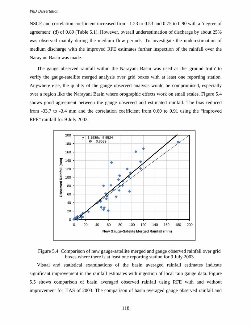
PhD Dissertation
118
NSCE and correlation coefficient increased from -1.23 to 0.53 and 0.75 to 0.90 with a ‘degree of
agreement’ (d) of 0.89 (Table 5.1). However, overall underestimation of discharge by about 25%
was observed mainly during the medium flow periods. To investigate the underestimation of
medium discharge with the improved RFE estimates further inspection of the rainfall over the
Narayani Basin was made.
The gauge observed rainfall within the Narayani Basin was used as the 'ground truth' to
verify the gauge-satellite merged analysis over grid boxes with at least one reporting station.
Anywhere else, the quality of the gauge observed analysis would be compromised, especially
over a region like the Narayani Basin where orographic effects work on small scales. Figure 5.4
shows good agreement between the gauge observed and estimated rainfall. The bias reduced
from -33.7 to -3.4 mm and the correlation coefficient from 0.60 to 0.91 using the “improved
RFE” rainfall for 9 July 2003.
Figure 5.4. Comparison of new gauge-satellite merged and gauge observed rainfall over grid boxes where there is at least one reporting station for 9 July 2003
Visual and statistical examinations of the basin averaged rainfall estimates indicate
significant improvement in the rainfall estimates with ingestion of local rain gauge data. Figure
5.5 shows comparison of basin averaged observed rainfall using RFE with and without
improvement for JJAS of 2003. The comparison of basin averaged gauge observed rainfall and
y = 1.1589x - 5.5524
R² = 0.8539
0
20
40
60
80
100
120
140
160
180
200
0 20 40 60 80 100 120 140 160 180 200
Obs
erve
d R
ainf
all (
mm
)
New Gauge-Satelite Merged Rainfall (mm)

PhD Dissertation
119
new gauge-satellite merged rainfall estimates for the four months of the 2003 monsoon shows
improvement in the overall estimation of rainfall but with a slight underestimation of medium
rainfall (Figure 5.5). The correlation coefficient increased from 0.02 to 0.92 and RMSE
decreased from 15.5 to 5.2 mm/day with the new gauge-satellite merged product compared with
unadjusted RFE rainfall estimates. Figure 5.6 shows the comparison of scatter plots of observed
and RFE rainfall estimates (without adjustment and with ingestion of local rain gauge) averaged
over the Narayani Basin.
There is however a negative percentage error of about 25% with underestimation of medium
rainfall in some days. The reason for this difference between the RFE and the gauge observed
rainfall may be attributed to the inherent systematic and random errors characteristic of SRE (Xie
et al., 2003; Hossain and Anagnostou, 2006). The underestimation of rainfall in some days may
be the reason for the difference in discharge simulation between observed and simulated using
the new gauge-satellite merged product where the overall underestimation of discharge was also
25%. Despite the difference in medium flows, with the new gauge-satellite merged product the
accuracy of prediction of daily peak flows is high. The average error above the threshold
discharge corresponding to the warning level is -7 % compared to -61% with unadjusted RFE.
0.0
10.0
20.0
30.0
40.0
50.0
60.0
70.0
152
160
168
176
184
192
200
208
216
224
232
240
248
256
264
272
Rai
nfal
l (m
m)
Time (Days)RFE Observed Rain
0.0
10.0
20.0
30.0
40.0
50.0
60.0
70.0
152
160
168
176
184
192
200
208
216
224
232
240
248
256
264
272
Rai
nfal
l (m
m)
Time (Days)
Improved RFE Observed Rain
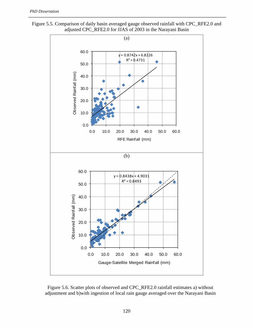
PhD Dissertation
120
Figure 5.5. Comparison of daily basin averaged gauge observed rainfall with CPC_RFE2.0 and adjusted CPC_RFE2.0 for JJAS of 2003 in the Narayani Basin
(a)
(b)
Figure 5.6. Scatter plots of observed and CPC_RFE2.0 rainfall estimates a) without adjustment and b)with ingestion of local rain gauge averaged over the Narayani Basin
y = 0.8742x + 6.8226R² = 0.4731
0.0
10.0
20.0
30.0
40.0
50.0
60.0
0.0 10.0 20.0 30.0 40.0 50.0 60.0
Obs
erve
d R
ainf
all (
mm
)
RFE Rainfall (mm)
y = 0.8438x + 4.9031R² = 0.8493
0.0
10.0
20.0
30.0
40.0
50.0
60.0
0.0 10.0 20.0 30.0 40.0 50.0 60.0
Obs
erve
d R
ainf
all (
mm
)
Gauge-Satellite Merged Rainfall (mm)

PhD Dissertation
121
To further test the improvement in performance with the improved RFE estimates the
GeoSFM model was calibrated using the improved RFE estimates instead of using the gauge
calibrated parameters. An improvement in the model performance was observed with the RMSE
decreasing from 1316 to 900, the normalized bias decreasing from -29% to -7% and a slight
increase in coefficient of correlation 0.90 to 0.92. Table 5.2 presents the statistical summary
comparing the simulated and gauge observed streamflow for JJAS of 2003 with the model
calibrated with gauge observed data and the improved RFE. Artan et al. (2008) and Hughes
(2006) had also indicated the need to recalibrate a hydrologic model when SRE are used as
rainfall inputs. From the current result it can be said that recalibration of the model is required
not only while running the model with SREs but also for new gauge-satellite merged rainfall
estimates. From this marked improvement in accuracy for flood prediction, we can infer that the
“improved RFE” are good for flood prediction in the Narayani Basin but has to be recalibrated
with the gauge-satellite merged rainfall estimates. The larger the number of ingested local
gauges, the better will be the flood prediction.
Table 5.2 Statistical summary of the comparison between simulated and observed streamflow for JJAS of 2003with RFE, gauge-satellite merged model calibrated with gauge observed data and gauge
satellite merged calibrated model.
RMSE
(m3/sec)
RMSE (%) Correlation
Coefficient
Normalized
Bias (%) Unsystematic Systematic
RFE 2750 19 81 0.73 -79
Gauge-satellite merged model
calibrated with gauge observed data 1316 43 57 0.90 -29
Gauge-satellite merged calibration
model 900 70 30 0.92 -7

PhD Dissertation
122
Figure 5.7 Observed and simulated hydrographs obtained when the model was calibrated with a) gauge observed rainfall and b) new gauge-satellite rainfall estimates.
5.4 Summary
In this chapter two approaches of bias-adjustment have been presented. The first set of bias-
adjustment is based on ratios derived from comparing the accumulated gauge observed rainfall
with RFE for the corresponding periods. Three bias-adjustments seasonal, monthly and a 7 day
0
2000
4000
6000
8000
10000
12000
14000
16000
152 162 172 182 192 202 212 222 232 242 252 262 272
Dis
char
ge (m
3 /sec
)
Time (Days)Observed Simulated
Gauge observed rainfall calibrated model
0
2000
4000
6000
8000
10000
12000
14000
16000
152 162 172 182 192 202 212 222 232 242 252 262 272
Dis
char
ge (m
3 /sec
)
Time (Days)Observed Simulated
Gauge satellite merged (Improved RFE) caibrated model
(a)
(b)

PhD Dissertation
123
moving average were derived. These bias-adjustments were applied to the RFE to obtain a new
set of improved RFE rainfall estimates. These improved RFE rainfall were applied to the
GeoSFM model which indicate improvement in flood prediction. The second approach is the
improvement in the rainfall estimates by ingesting additional local rain gauge data into the RFE
algorithm by expanding the GTS data input. When the model calibrated with the gauge
observation was run with the improved rainfall estimates considerable improvement in flood
prediction was achieved. However, there seemed to be some discrepancy in the medium flow
estimation. Therefore keeping in mind the inherent errors in the SREs the model was recalibrated
with improved RFE. The recalibrated model with new gauge-satellite merged rainfall estimates
showed further improvement in the simulation of flows. Overall, findings from this study
indicate that the accuracy SRE can be improved by applying a bias-adjustment. Prediction of
discharge using bias-adjusted rainfall estimates can improve the accuracy discharge prediction
with considerable increase in the predictive capability of flood prediction for which the
hydrological model needs to be recalibrated.
References
Artan, G.A., Gadain, H., Smith, J.L., Asante, K., Bandaragoda, C.J., Verdin, J.P. (2007a)
Adequacy of satellite derived rainfall data for streamflow modelling. Nat. Hazards, 43, 167-
185.
Hay, L.; Clark, M.; Wilby, R.; Gutowski, W.; Leavesley, G.; Pan, Z., Arritt, R.; and Takle, E.:
(2002) Use of regional climate model output for hydrologic simulations, J. Hydrometeorol.,
224:3, pp. 571–590.
Hossain, F. and Anagnostou, E.N.: (2006) Assessment of a multidimensional satellite rainfall
error model for ensemble generation of satellite rainfall data. IEEE Geoscience and Remote
Sensing Letters, Vol. 3, No. 3: pp. 419-423.
Hughes, D.A. (2006) Comparison of satellite rainfall data with observations from gauging station
networks. J. Hydrol., 327, 399–410.

PhD Dissertation
124
Ines, A.V.M. and Hansen J.W.: (2006) Bias correction of daily GCM rainfall for crop simulation
studies. Agricultural and Forest Meteorology. 138, pp. 44–53
National Oceanic and Atmospheric Administration (NOAA), 2009. The NOAA Climate
Prediction Center CPC RFE2 rainfall estimation software for the Hindu Kush and Mekong
regions of Asia.
Piani, C.; Haerter, J.O.; and Coppola, E.: (2010) Statistical bias correction for daily precipitation
in regional climate models over Europe. Theor Appl Climatol. 99: pp. 187-192.
Terink, W.; Hurkmans, W.L.; Torfs, P.J.J.F.; and Uijlenhoet, R.; (2010) Evaluation of a bias
correction method applied to downscaled precipitation and temperature reanalysis data for
the Rhine basin. Hydrol. Earth Syst. Sci. Discuss., 7, pp. 221–267
Terink, W.; Hurkmans, W.L.; Torfs, P.J.J.F.; and Uijlenhoet, R.; (2009) Evaluation of a bias
correction method applied to downscaled precipitation and temperature reanalysis data for
the Rhine basin. Hydrol. Earth Syst. Sci., 14, pp. 687–703.
Xie, P., Arkin, P.A., 1996. Analyses of global monthly precipitation using gauge observations,
satellite estimates and numerical model predictions. J. Clim. 9, 840–858.
Xie, P.; Yarosh, Y.; Love, T. ; Janowiak, J E.; and Arkin, PA. (2002) A Real-Time Daily
Precipitation Analysis Over South Asia Preprints, 16th Conference of Hydrology, Orlando,
FL, American Meteorological Society 12-17 January 2002.

PhD Dissertation
125
CHAPTER 6
6 CONCLUSIONS AND RECOMMENDATIONS
The verification of satellite based rainfall estimates, bias-adjustment and application of the
rainfall estimates into hydrological modeling for flood prediction are the main aspects of this
research. SRE is a new technology for Nepal and prior to this research there has been very little
application of SRE into hydrological modeling. This research is the first to conduct a detailed
verification of the SRE over Nepal to understand the strengths and weakness of the now more
easily available global satellite-based rainfall products. As there is no operational flood
forecasting and warning system in place in Nepal this study has provided an opportunity to
explore the application of remotely sensed data for streamflow estimation and flood forecasting.
Accurate rainfall estimations are essential for timely flood forecasting and warning. In many
regions operational flood forecasting has traditionally been relied upon by a dense network of
rain gauges or ground-based rainfall measuring radars that report in real time. In Nepal, like
many other developing countries, the hydrometeorological station networks are sparse and
rainfall data are available only after a significant delay. Due to the limited spatial coverage of
ground based gauges, unavailability of real-time rainfall data, and constraint in technical and
financial resources, operational flood forecasting is yet to be initiated. Thus, SRE is considered
as an appropriate approach for Nepal to predict and forecast rainfall-induced runoff that may
produce flooding. Two high resolution SREs were selected for verification in this research. The
NOAA CPC_RFE2.0 (RFE) mutli-satellite gauge merged rainfall estimates and the JAXA
GSMaP_MVK+ (GSMaP) global rainfall estimates both available at a 0.1 degree x 0.1degree
spatial resolution on a daily basis. The RFE uses merging technique which increases the
accuracy of the rainfall estimates by reducing significant bias and random error compared to
individual precipitation data sources thereby adding value to rain gauge interpolations GSMaP
includes a Kalman filtering technique. The RFE provides near real time rainfall estimates over
South Asia and the GSMaP has a near real time product with a 4 hr latency which makes it
attractive for flood forecasting in Nepal. In the research the RFE estimates from 2002 to 2006
and GSMaP from 2003 to 2006 have been used for verification. Gauge observed rainfall data
from 176 stations made available from the DHM of the Government of Nepal were used to

PhD Dissertation
126
conduct the validation over Nepal considering various levels of validation, whole country as a
homogeneous region, various physiographic regions and in river basins. The quality of the
estimates in terms of spatial distribution and amount was assessed by using the standard
statistical verification technique by comparing bias, RMSE, correlation coefficient,
multiplicative bias, percentage error, POD and FAR values for each set of validation data. As
Nepal has a complex topography with elevation ranging from 60 m to 8848m within a short
horizontal distance of less than 200 km the verification of SREs were made in various
physiographic regions to better understand the performance of the rainfall estimates in such
complex topography. As the final objective of this research is to assess the applicability of SREs
into hydrological modeling for flood prediction rainfall verifications were also conducted at a
basin level considering different basin sizes.
The USGS GeoSFM was used to simulate the rainfall-runoff processes in two river basins
Bagmati and Narayani using the gauge observed and RFE. The GeoSFM model was calibrated
and validated using the gauge observed data. RFE estimates were applied to simulate the
discharge. Comparison of the observed and simulated discharge using the gauge observed data
was very good indicating the suitability of GeoSFM into flood forecasting. However when the
model was run with RFE the performance of the model deteriorated sharply indicating the need
for correcting the rainfall estimates prior to further application.
As the SREs were found to underestimate bias-adjustment of the estimates were made. Two
approaches of bias-adjustment, ratio based bias-adjustment at various temporal accumulations
seasonal, monthly and 7-day moving average and gauge-satellite merged rainfall estimates were
developed and assessed. The application of bias-adjusted rainfall estimates into the GeoSFM
model showed marked improvement in flood predictability with all three ratio based bias-
adjustment. However, the monthly bias-adjustment seemed to perform slightly better than the
other two with better flood predictions showing a low peak flow error. As a second approach a
new set of rainfall estimates were produced by ingesting the locally available rain gauge data
into the RFE algorithm which when applied to the GeoSFM showed better flood predictions.
However, the current research has indicated the need to recalibrate the GeoSFM with the new
sets of rainfall estimates to come up with improved flood predictions.

PhD Dissertation
127
6.1 Satellite-Based Rainfall Estimate Validation
The country level validation results indicate the RFE and GSMaP provides reasonable
rainfall estimates over the Central Himalayas of Nepal but needs to be improved before it can be
implemented for operational flood forecasting. The physiographic level validation has shown
that performance of the SRE was better in flatter terrain compared to mountainous areas. Due to
orographic effects in the mountainous areas the performance of the RFE seems to deteriorate. In
the monsoon period there was underestimation of rainfall with a high negative bias. While in the
rain shadow areas there was overestimation of the rainfall indicating a positive bias. The major
findings and recommendations are given below.
Findings:
• The area average annual gauge observed rainfall over whole of Nepal is 1433 mm,
RFE is 1021 mm and GSMaP is 748 mm for 2003 to 2006 period with an annual bias
of 421 mm with RFE and 685 mm with GSMaP.
• On an annual basis there is 29% underestimation by rainfall by RFE and 48% by
GSMaP for the four years period from 2003 to 2006.
• There is a negative bias of 1.1 mm day-1 with RFE and 1.9 mm day-1 with GSMaP.
• Both the SREs have significant correlation. There is higher correlation with GSMaP
(0.75) than RFE (0.71).
• There is higher negative bias in averaged monsoon (JJAS) rainfall over whole of
Nepal with RFE and GSMaP. With RFE there is -2.9 mm day-1 and with GSMaP -5.0
mm day-1 with the correlation of 0.72 and 0.79 respectively.
• In high intensity rainfall areas example in Pokhara valley there is underestimation of
as much as 2000 mm while in rainshadow areas of Mustang there is over a positive
bias with overestimation. The positive bias with RFE is larger as compared to with
GSMaP.
• The performance of SREs is better in the flatter terrain and deteriorates with increase
in elevation.
• The limitation of RFE is that at present it cannot register more than a certain amount
of rainfall in 24 hours, which is not enough in the case of monsoon depression and

PhD Dissertation
128
monsoon trough in Nepal. RFE does not account for orographic aspects of rainfall.
GSMaP also does not have orographic corrections.
• Three ratio bias-adjustments seasonal, monthly and a 7-day moving average have
been derived and applied to develop corrected rainfall estimates. The correction ratios
obtained for the monsoon season is 1.82 and monthly for June, July, August and
September are 1.99, 2.0, 1.58, and 1.82.
6.2 Hydrological Modelling Using Satellite-Based Rainfall Estimates
The GeoSFM hydrological model using gauge observed rainfall data and globally available soil
and land cover datasets—the Digital Soil Map of the World by FAO and the USGS Global Land
Cover resulted in accurate discharge prediction in the Bagmati and Narayani Basins. The
GeoSFM predicted the flows accurately when observed rain gauge data have been applied and
calibrated indicating reliable application to flood forecasting with good quality of rainfall
estimates. However, when the RFE was used in the GeoSFM model as the rainfall input the
performance of the model deteriorated with significant underestimation of flows. Although the
satellite based rainfall products are capable of detecting a particular rainfall event within the
magnitude of the computed discharge is much lower in the RFE driven model compared to the
model with gauged observed rainfall. The NSCE was very low however the correlation was still
over 0.75 indicating the applicability of improvement with a bias-adjustment.
Bias-adjustments based on ratios comparing the accumulated gauge observed rainfall with
RFE for the corresponding periods were derived on a seasonal, monthly and a 7 day moving
average basis. These bias-adjustments were applied to the RFE to obtain a new set of improved
RFE rainfall estimates. These improved RFE rainfall were applied to the GeoSFM model which
indicate improvement in flood prediction. The second approach is the improvement in the
rainfall estimates by ingesting additional local rain gauge data into the RFE algorithm by
expanding the GTS data input. When the model calibrated with the gauge observation was run
with the improved rainfall estimates considerable improvement in flood prediction was achieved.
However, there seemed to be some discrepancy in the medium flow estimation. Therefore,
keeping in mind the inherent errors in the SREs the model was recalibrated with improved RFE.
The recalibrated model with new gauge-satellite merged rainfall estimates showed further
improvement in the simulation of flows.
The major findings are given below.

PhD Dissertation
129
• SREs highly under predicts peak discharge.
• The accuracy flood prediction can be improved by applying a bias-adjustment.
• The bias-adjustment derived on a monthly basis yielded better improvement in the flood
predictability compared to other adjustments.
• The application of improved RFE obtained by merging local rain gauge data with SREs
in the model yielded the best result of flood prediction for which the hydrological model
needs to be recalibrated.
6.3 Recommendations and Future Perspectives
This research reveals that the satellite estimates need to be improved over the Himalayas
particularly in areas of orographic influence. This improvement may be made by correction in
the algorithm by incorporating the orographic effects into the rainfall estimation. One way of
doing this may be by adjusting the GOES Precipitation Index (GPI) for the Geo-stationary input
data so as to incorporate a variable brightness temperature to rain rate conversion in the HKH
region. Passive microwave measurements depend strongly on the relations between the
hydrometeor size distribution, types and the rain intensity. Therefore, it is essential to obtain
information about the hydrometeor sizes for achieving reasonable accuracy of the precipitation
intensities.
The basic algorithms, for example in the RFE ignores the GTS data when it reports more
than 200 mm, should be modified and included in the heavy rainfall event. There are many
events in a year when rainfall exceed 200 mm per day in Nepal. Another example is the GSMaP
algorithm where a statistical database of precipitation vertical profiles classified into 10 types are
used, but currently does not reflect profiles of localized precipitation systems. The profiles of
heavy orographic rainfall in the Himalayas are unique and largely different from those in the
database, which could be considered to be improved for better rainfall estimation.
The current verification has been conducted using limited data. Further verification may be
conducted with additional data and products and using finer temporal and spatial scales for the
utility of SRE in flood forecasting. The bias-adjustment technique could be further explored as
additional data becomes available. Longer sets of concurrent data between the SRE and gauge

PhD Dissertation
130
observation may provide a better estimate of bias correction which could be applied for
improved flood forecasting.
Finally, bias-adjusted SREs appear to be an effective and viable means to achieve an estimate
of precipitation over Nepal. The GeoSFM model with the bias-adjustments derived from this
study will be evaluated in the coming monsoon season in near real time for the Narayani Basin
for flood prediction.
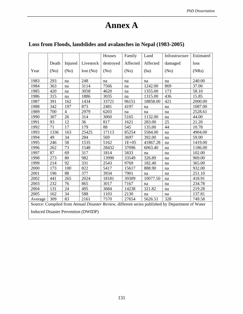
PhD Dissertation
131
Annex A
Loss from Floods, landslides and avalanches in Nepal (1983-2005)
Year
Death
(No)
Injured
(No)
Livestock
lost (No)
Houses
destroyed
(No)
Family
Affected
(No)
Land
Affected
(ha)
Infrastructure
damaged
(No)
Estimated
loss
(NRs)
1983 293 na 248 na na na na 240.001984 363 na 3114 7566 na 1242.00 869 37.001985 420 na 3058 4620 na 1355.00 173 58.101986 315 na 1886 3035 na 1315.00 436 15.851987 391 162 1434 33721 96151 18858.00 421 2000.001988 342 197 873 2481 4197 na na 1087.001989 700 4 2979 6203 na na na 2528.611990 307 26 314 3060 5165 1132.00 na 44.001991 93 12 36 817 1621 283.00 25 21.201992 71 17 179 88 545 135.00 44 10.781993 1336 163 25425 17113 85254 5584.00 na 4904.001994 49 34 284 569 3697 392.00 na 59.001995 246 58 1535 5162 1E+05 41867.28 na 1419.001996 262 73 1548 28432 37096 6063.40 na 1186.001997 87 69 317 1814 5833 na na 102.001998 273 80 982 13990 33549 326.89 na 969.001999 214 92 331 2543 9769 182.40 na 365.002000 173 100 822 5417 15617 888.90 na 932.002001 196 88 377 3934 7901 na na 251.102002 441 265 2024 18181 39309 10077.50 na 418.912003 232 76 865 3017 7167 na na 234.782004 131 24 495 3684 14238 321.82 na 219.282005 162 34 588 1103 2130 na na 137.81Average 309 83 2161 7570 27654 5626.51 328 749.58Source: Compiled from Annual Disaster Review, different series published by Department of Water
Induced Disaster Prevention (DWIDP)

PhD Dissertation
132
ANNEX 2
List of Rainfall Stations used for the research
S.No Longitude Latitude Station Name
1 80.58 29.30 Dadeldhura
2 80.60 28.68 Dhangadhi
3 82.17 29.28 Jumla
4 84.00 28.22 Pokhara Airport
5 83.43 27.52 Bhairhawa Airpo
6 84.98 27.17 Simara Airport
7 85.37 27.70 Kathmandu Airpo
8 86.50 27.32 Okhal Dhunga
9 87.67 27.35 Taplejung
10 87.35 26.98 Chandpur
11 87.27 26.48 Biratnagar Airp
12 80.50 29.65 Kakerpakha
13 80.42 29.55 Baitadi
14 80.35 28.68 Belauri
15 80.47 29.53 Satbanj
16 80.87 29.62 Pipalkot
17 81.32 29.38 Bajura
18 81.13 29.00 Katai
19 81.45 28.95 Asara
20 80.92 28.75 Sandepani
21 81.12 28.97 Bangga
22 81.20 29.38 Khaptad
23 80.82 28.57 Sitapur
24 80.68 29.12 Kola Gaon
25 81.28 29.15 Mangalsen
26 81.77 29.32 Thirpu
27 82.32 29.28 Guthi
28 81.60 29.13 Sheri Ghat
29 82.15 29.55 Gam Shree
30 81.90 29.20 Magma

PhD Dissertation
133
31 81.63 29.23 Bijayapur
32 81.33 28.78 Jamu
33 82.20 28.70 Jajarkot
34 82.12 28.02 Kusum
35 81.35 28.17 Gulariya
36 81.58 28.78 Bale
37 81.10 28.43 Rajapur
38 81.72 28.27 Naubasta
39 81.70 28.35 Shyano Shree
40 81.90 28.05 Baijapur
41 81.35 28.43 Bargadaha
42 82.28 28.98 Maina Gaon
43 82.63 28.60 Rukumkot
44 82.63 28.30 Libang
45 82.87 28.10 Bijuwar Tar
46 82.12 28.22 Nayabasti
47 82.50 28.05 Ghorahi
48 82.53 27.70 Koilabas
49 82.28 28.30 Luwamjula
50 83.65 28.48 Tatopani
51 83.88 28.82 Ranipauwa
52 83.88 29.05 Ghami
53 83.97 29.18 Mustang
54 83.75 28.18 Karki Neta
55 83.10 28.40 Bobang
56 83.22 28.60 Gurja
57 83.73 28.40 Ghorapani
58 83.65 28.03 Tribeni
59 83.40 28.38 Darbang
60 83.57 28.15 Rangkhami
61 83.78 28.97 Samar
62 83.68 28.90 Samoa
63 83.60 28.47 Bega
64 83.48 28.38 Kuhun

PhD Dissertation
134
65 83.38 28.57 Baghara
66 83.62 28.13 Sirkon
67 83.43 27.95 Ridi Bazar
68 84.05 27.68 Beluwa
69 83.67 27.53 Parasi
70 83.87 27.58 Dhumkibas
71 83.05 27.77 Pattharkot
72 83.27 28.17 Musikot
73 82.80 27.68 Bhagwanpur
74 83.80 27.87 Garakot
75 83.28 27.47 Lumini
76 84.90 28.37 Jagat
77 84.62 28.67 Larke Samdo
78 84.35 28.13 Kunchha
79 84.42 27.93 Bandipur
80 83.82 28.27 Bhadaure
81 84.28 27.97 Damauli
82 83.97 28.27 Lamachaur
83 84.02 28.67 Manang
84 83.80 28.38 Ghandruk
85 84.62 28.20 Gharedhunga
86 84.10 28.37 Siklesh
87 83.77 27.98 Walling
88 84.13 27.87 Rumjakot
89 83.75 28.27 Sallyan
90 83.78 28.27 Pamdur
91 84.53 27.58 Jhawani
92 85.13 27.55 Chisapani
93 85.00 27.28 Amlekhganj
94 85.17 27.18 Nijgadh
95 85.38 27.02 Ramoli
96 85.15 27.62 Markhu
97 84.87 27.00 Birganj
98 85.17 27.42 Makwanpur
99 84.82 27.55 Beluwa

PhD Dissertation
135
100 85.00 27.03 Kalaiya
101 85.02 26.92 Kolbhi
102 85.13 26.95 Chuntaha
103 84.98 27.43 Rajaiya
104 85.38 28.28 Timure
105 84.82 28.05 Aru Ghat
106 84.93 27.87 Dhading
107 85.87 27.87 Gumthang
108 85.62 27.80 Nawalpur
109 85.72 27.78 Chautara
110 85.20 27.68 Thankot
111 85.60 27.95 Sarmathang
112 85.57 27.87 Dubachaur
113 85.57 27.78 Baunepati
114 85.65 27.70 Mandan
115 85.72 27.63 Dolal Ghat
116 85.63 27.92 Dhap
117 85.90 27.78 Barabhise
118 85.75 27.57 Pachuwar Ghat
119 85.48 27.75 Sankhu
120 85.52 27.58 Khopasi (Panauti)
121 85.42 27.67 Bhaktapur
122 85.32 28.17 Thamchit
123 85.55 28.00 Tarkhe Ghyang
124 85.42 27.70 Changu Narayan
125 85.33 27.60 Chapa Gaon
126 85.72 27.70 Sanga chowk
127 85.78 27.70 Thokarpa
128 85.42 27.77 Sundarijal
129 85.28 27.58 Lele
130 85.25 27.68 Naikap
131 85.42 27.75 Sundarijal
132 85.63 27.90 Dhap
133 85.25 27.75 Nararjun

PhD Dissertation
136
134 86.10 27.68 Nagdanda
135 86.05 27.67 Charikot
136 86.05 27.52 Melung
137 86.17 27.18 Bahun Tilpung
138 85.67 27.08 Pattharkot (east)
139 85.92 27.03 Tulsi
140 86.17 26.92 Chisapani Bazar
141 85.82 27.45 Nepalithok
142 85.50 27.33 Hariharpur Ghad
143 85.78 26.88 Gausala
144 85.57 26.87 Malangwa
145 86.08 27.47 Manthali
146 86.72 27.70 Chaurikhark
147 86.57 27.43 Pakarnas
148 86.75 27.35 Aisealukhark
149 86.42 27.48 Mane Bhanjyang
150 86.43 27.13 Kurule Ghat
151 86.83 27.03 Khotang Bazar
152 86.22 26.65 Siraha
153 86.58 27.50 Salleri
154 86.80 27.22 Diktel
155 86.38 27.55 Sirwa
156 86.90 26.60 Barmajhiya
157 87.28 27.55 Num
158 87.28 27.13 Leguwa Ghat
159 87.23 27.03 Munga
160 87.33 26.93 Mul Ghat
161 87.15 26.93 Tribeni
162 87.38 26.62 Haraincha
163 87.17 26.82 Chatara
164 87.42 27.77 Chepuwa
165 87.22 27.28 Tumlingtar
166 87.17 26.97 Machuwaghat
167 87.15 27.37 Dingla
168 87.78 27.55 Lungthung

PhD Dissertation
137
169 87.78 27.48 Taplethok
170 87.93 27.20 Memeng Jagat
171 87.70 26.67 Damak
172 87.98 26.63 Anarmani Birta
173 88.03 26.88 Himali Gaon
174 88.05 26.57 Chandra Gadhi
175 87.97 26.68 Sanishare
176 87.60 27.35 Dovam