Embed Size (px)
Citation preview
Transportation 13: 163-181 (1986) 163 © Martinus Nijhoff Publishers, Dordrecht - Printed in the Netherlands
Biases in response over time in a seven-day travel diary
THOMAS E GOLOB & HENK MEURS Bureau Goudappel Coffeng BV, Parkweg 4, Deventer, the Netherlands
Abstract. Data from multi-day travel or activity diaries might be biased if recording inaccuracies
and tendencies for respondents to skip certain types of trips or activities increases (or decreases)
from day-to-day over the diary period. One objective of the research reported here is to test for
such temporal biases in a seven-day travel diary. A second objective is to calculate correction fac-
tors which can be applied to the data in the case that biases are found. The analyses were conduct-
ed using regression and analysis-of-variance techniques. The variables investigated included total
trips per day, total travel time per day, and trips per day by various modes (such as walking, car
driver and car passenger). Results showed that most biases per capita statistics are due to increases
over t ime in the percentage of respondents reporting no travel at all for an entire day. However,
even after accounting for this bias by measuring statistics in terms of "per mobile person", there
remains a decrease over time of about 3.5 percent per day in the reporting of walking trips. This
appears to be the main factor in the overall bias of about one percent per day in total trips per
mobile person per day. No significant differences were found among population segments in terms
of the levels of their biases.
Objectives and Scope
Travel diaries, in which respondents record salient facts about the trips they make over a fixed period of time, provide the fundamental data for most studies of travel behaviour. Usually, the time period for such diaries is one or two days. It is quite possible that this emphasis on only one or two days of travel and related activities has severely restricted the subject matter and the methodologies of travel-behaviour studies. Indeed, several authors have point- ed out the limitations imposed by diaries of one or two days (e.g., Scheuch, 1972; Goodwin, 1979).
Extending the recording periods for travel and activity diaries, perhaps to seven days or more, permits the study of day-to-day variations in travel be- haviour. Focus can be placed more effectively on activity patterns which typi- cally occur in cycles of multi-day duration (e.g., weekly). Also, time and money expenditure patterns (so-called budgets) can be more effectively analysed, be- cause one or two days is in general too short a time for observing overall expen- ditures. Examples of studies addressing these topics using extended-period data are provided by Bentley et al. (1977), van der Hoorn (1979), Lyn & Ruchon (1979), Hanson & Hanson (1979), Jones et al. (1980), Hanson (1980), Clarke et al. (1981), and Koppelman & Pas (1984).
However, it is possible that diary data of extended durations contain more
164
biases than short-duration data. This would be true if recording inaccuracies and tendancies to skip certain types of trips or activities increased with time. Such biases, usually attributed to respondent fatigue or diminished motiva- tion, have been proposed by Szalai (1972) and Br6g & Meyburg (1980, 1982), among others. Empirically, temporal biases were found in fourteen-day data by Lyn & Ruchon (1979) and in seven-day data by Clarke et al. (1981), but Han- son & Huff (1981) found no such bias in thirty-five day data. The general lack of empirical evidence and the conflicting results from the few studies which have addressed the issue has led to a reluctance among data collectors to use diary periods beyond two days (e.g., Br6g, 1982).
The objectives of the present study are to test for temporal biases in seven- day diaries and to calculate correction factors which can be applied to data in the case that biases are found. Temporal is a key word in defining the limita- tions of this study: The study is not concerned with the accuracy of the diary instrument as applied on each respondents first day of the diary period. The biases investigated concern diary sequence days two through seven relative to the first day's reporting.
The data
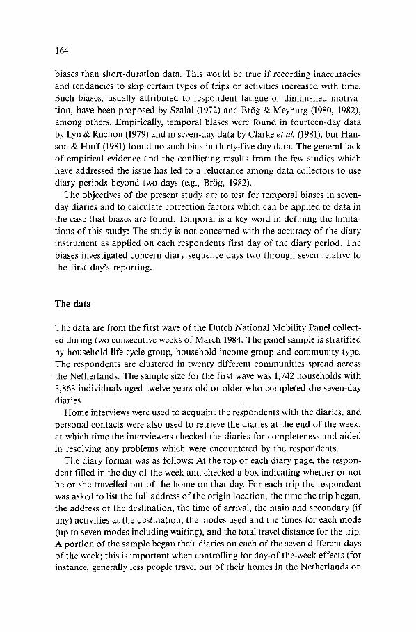
The data are from the first wave of the Dutch National Mobility Panel collect- ed during two consecutive weeks of March 1984. The panel sample is stratified by household life cycle group, household income group and community type. The respondents are clustered in twenty different communities spread across the Netherlands. The sample size for the first wave was 1,742 households with 3,863 individuals aged twelve years old or older who completed the seven-day diaries.
Home interviews were used to acquaint the respondents with the diaries, and personal contacts were also used to retrieve the diaries at the end of the week, at which time the interviewers checked the diaries for completeness and aided in resolving any problems which were encountered by the respondents.
The diary format was as follows: At the top of each diary page, the respon- dent filled in the day of the week and checked a box indicating whether or not he or she travelled out of the home on that day. For each trip the respondent was asked to list the full address of the origin location, the time the trip began, the address of the destination, the time of arrival, the main and secondary (if any) activities at the destination, the modes used and the times for each mode (up to seven modes including waiting), and the total travel distance for the trip. A portion of the sample began their diaries on each of the seven different days of the week; this is important when controlling for day-of-the-week effects (for instance, generally less people travel out of their homes in the Netherlands on
165
Sundays, while Fridays and Thursdays tend to exhibit the most travel). Ac- counting for day-of-the-week effects is complicated by the fact that the sub- samples of respondents beginning their diaries of the different days were not of equal size. Of the 3,863 respondents, only 53 (1.3%) began on Monday, 890 (23.0%) on Tuesday, 727 (18.8%) on Wednesday, 801 (20.7%) on Thursday, 728 (18.8% on Friday), 401 (10.4%) on Saturday, and 263 (6.8%) on Sunday. Thus, looking only at the raw data aggregated for the entire sample, a reduction in trip making would be apparent for the sixth sequence day due only to the fact that a large proportion of the sample had Sunday as a sixth day (these were
the subsample beginning on Tuesday).
Overall mobility levels
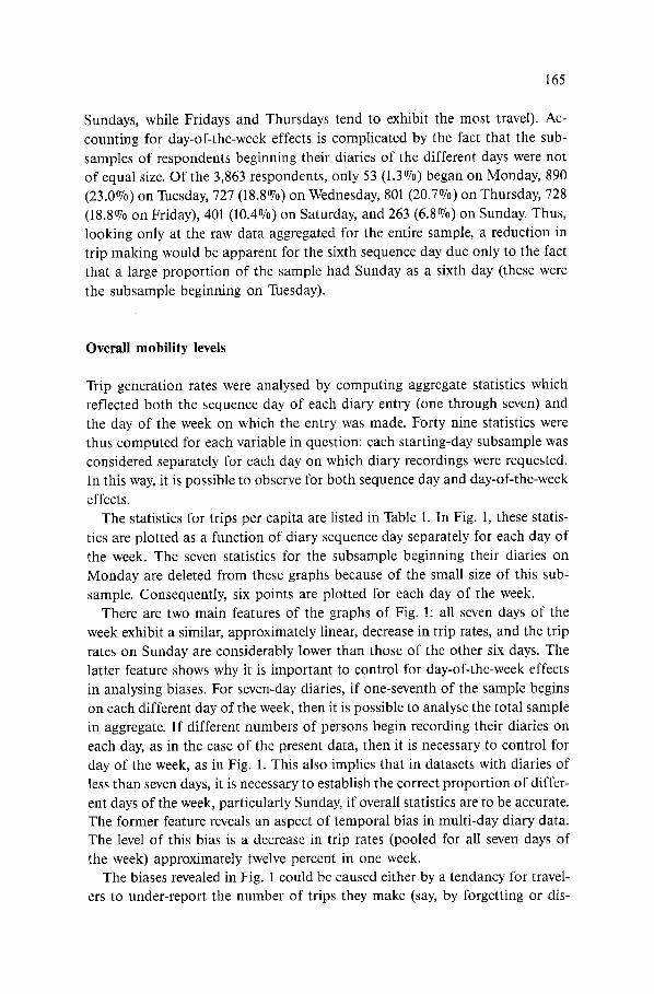
Trip generation rates were analysed by computing aggregate statistics which reflected both the sequence day of each diary entry (one through seven) and the day of the week on which the entry was made. Forty nine statistics were thus computed for each variable in question: each starting-day subsample was considered separately for each day on which diary recordings were requested. In this way, it is possible to observe for both sequence day and day-of-the-week
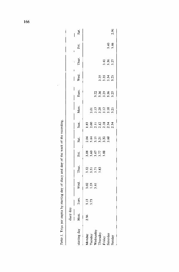
effects. The statistics for trips per capita are listed in Table 1. In Fig. 1, these statis-
tics are plotted as a function of diary sequence day separately for each day of the week. The seven statistics for the subsample beginning their diaries on Monday are deleted from these graphs because of the small size of this sub- sample. Consequently, six points are plotted for each day of the week.
There are two main features of the graphs of Fig. !: all seven days of the week exhibit a similar, approximately linear, decrease in trip rates, and the trip rates on Sunday are considerably lower than those of the other six days. The latter feature shows why it is important to control for day-of-the-week effects in analysing biases. For seven-day diaries, if one-seventh of the sample begins on each different day of the week, then it is possible to analyse the total sample in aggregate. If different numbers of persons begin recording their diaries on each day, as in the case of the present data, then it is necessary to control for day of the week, as in Fig. 1. This also implies that in datasets with diaries of less than seven days, it is necessary to establish the correct proportion of differ- ent days of the week, particularly Sunday, if overall statistics are to be accurate. The former feature reveals an aspect of temporal bias in multi-day diary data. The level of this bias is a decrease in trip rates (pooled for all seven days of the week) approximately twelve percent in one week.
The biases revealed in Fig. 1 could be caused either by a tendancy for travel- ers to under-report the number of trips they make (say, by forgetting or dis-
Ta
ble
1.
Tri
ps p
er c
apit
a by
sta
rtin
g da
y o
f di
ary
and
day
of t
he w
eek
of t
he r
ecor
ding
.
diar
y da
y
star
ting
day
M
ort.
T
ues.
W
ed.
Th
ur.
F
ri.
Sat
. S
un.
Mo
n.
Tue
s.
Wed
. T
hu
r.
Fri
. S
at.
Mo
nd
ay
2.96
3.
13
3_02
3.
32
3.08
2.
04
1.83
Tue
sday
3.
73
3.53
3.
51
3.60
3.
14
2.00
3.
01
Wed
nesd
ay
3.61
3.
71
3.67
3.
15
2.11
3.
13
3.22
T
hurs
day
3.83
3.
77
3.21
2.
12
3.28
3.
36
3.35
Fri
day
' 3.
88
3.32
2.
18
3.12
3.
29
3.35
3.
41
Sat
urda
y 3.
60
2.34
3.
18
3.56
3.
34
3.36
3.
40
Sun
day
2.34
3.
21
3.25
3.
23
3.27
3.
46
2.91
167
Trips per capita
4 . 0
3.~
3.4
2 . !
2.4
1 . 5
1 . 0
0 . 5
o.°~..'T ......... • °, • .o o ~
• "'L. ~ , . I ~
~ O "" ' " . . • ~ . " : ' ' " " •
~Ii" -+i+,. . ~ , .~ "~+r,,. ,,.,.@,+ e
• -4---*- -ii- monday
..... tuesday
- - - - - wednesday
............. thursday
. . . . . friday
@ + ~ + + saturday
sunday
Day in diary sequence
Fig. 1. Trips per capita by day in diary sequence parameterised by day of the week (small sample starting on Monday is excluded).
regarding certain short trips) or by an increase in the number of persons who report no trips at all on a given day.
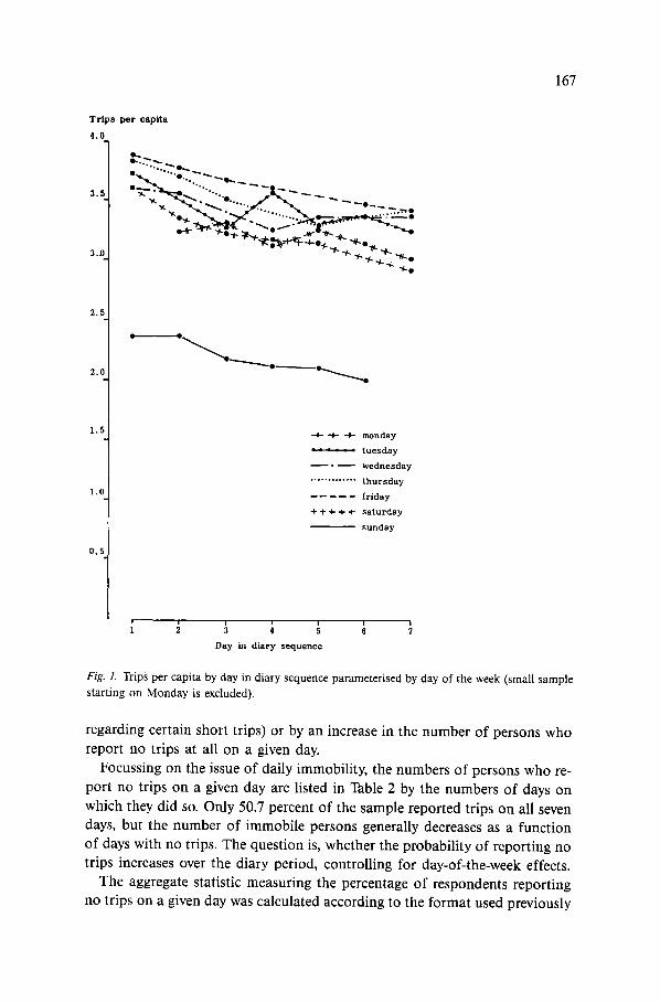
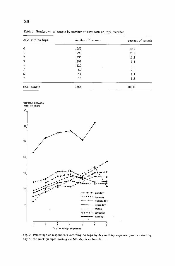
Focussing on the issue of daily immobility, the numbers of persons who re- port no trips on a given day are listed in Table 2 by the numbers of days on
which they did so. Only 50.7 percent of the sample reported trips on all seven days, but the number of immobile persons generally decreases as a function of days with no trips• The question is, whether the probability of reporting no trips increases over the diary period, controlling for day-of-the-week effects•
The aggregate statistic measuring the percentage of respondents reporting no trips on a given day was calculated according to the format used previously
168
Table 2. Breakdown of sample by number of days with no trips recorded.
days with no trips number of persons percent of sample
0 1959 50.7
1 990 25.6
2 393 10.2
3 209 5,4
,4 120 3.1
5 82 2.1
6 51 1.3
7 59 1.5
total sample 3863 100.0
percent persons
with no t r i p s
35
30.
25
A¢ o - X
. '"3¢'. . _ O - b ~ + -~-O,~. "" " ' M ' ~ O
l f i ~,( ~ j . . " A ~ . .O -4--~F- ~
x o + + ' ~ ° ~ _ ~ . " % ~ ~ o - ' ' . - +.~ ~ ~ . ~ ..... " - ~ 8 ~ ~ ~- - .-..-.
o,.~-~ .~ ~.~.,,-,~. ° ~ , ~ .~ "~.__.-~-.: i x " .....' 1 "-0--- .~ o..-----'~.
~ . ,~,,:.','-- -- _ r ~ / % 1o a ~.7....-Z-e.. • • ~ ~
o t " - ,.5o / • ~ ~...~. -4- -N- -41- monday
tuesday
0"" ~ • - wednesday
5 ............. thursday
..... f r iday
-{- -4- d- + + saturday
- - sunday
D a y i n d i a r y sequence
Fig. 2. Percentage of respondents recording no trips by day in diary sequence parameterised by
day of the week (sample starting on Monday is excluded),
Tab
le 3
. P
erce
ntag
e of
res
pond
ents
rec
ordi
ng n
o tr
ips
by s
tart
ing
day
of d
iary
and
day
-of-
the-
wee
k of
rec
ordi
ng.
diar
y da
y
star
ting
day
M
on.
Tue
s.
Wed
. T
hur.
F
ri.
Sat
. S
un.
Mo
n.
Tue
s.
Wed
. T
hu
r.
Fri
. S
at.
Mo
nd
ay
9.4
9.4
13.2
7.
5 17
.0
32.1
34
.0
Tue
sday
9.
1 11
.2
11.1
11
.3
14.7
31
.5
16.0
Wed
nesd
ay
10.0
10
.5
11.6
16
.1
26.1
15
.4
12.2
T
hu
rsd
ay
6.6
9.4
15.9
29
.1
13.5
12
.0
13.0
F
rida
y 8.
0 13
.2
28.3
15
.1
12.1
12
.6
11.5
S
atur
day
12.5
26
.7
14.5
13
.0
13.7
17
.7
14.2
S
unda
y 22
.1
12.2
12
.2
14.8
15
.6
14.8
19
.4
Ta
ble
4.
Tri
ps p
er m
obil
e pe
rso n
(pe
rson
mak
ing
tri
ps o
n t
he
day
in q
ues
tio
n)
by s
tart
ing
day
an
d d
ay-o
f-th
e-w
eek
of
reco
rdin
g.
diar
y da
y
star
ting
day
M
on.
Tue
s.
Wed
. T
hu
r.
Fri
. S
at.
Sun
. M
on
. T
ues
. W
ed.
Th
ur.
F
ri.
Sat
.
Mo
nd
ay
3.27
3.
46
3.48
3.
59
3.70
3.
00
2.77
Tu
esd
ay
4.11
3.
97
3.95
4.
06
3.68
2.
92
3.59
W
edn
esd
ay
4.01
4.
14
4.14
3.
75
2.85
3.
70
3.67
Th
urs
day
4.
10
4.16
3.
82
2.99
3.
79
3.81
3.
85
Fri
day
4.21
3.
83
3.03
3.
67
3.75
3.
84
3.85
S
atur
day
4.11
3.
20
3.83
4.
09
3.88
4.
08
3.96
Su
nd
ay
3.00
3.
65
3.70
3.
79
3.87
4.
06
3.61
171
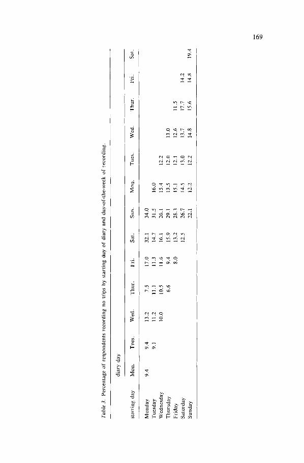
for trips per capita by day. These statistics are listed in Table 3 and are graphed by sequence day by day of the week in Fig. 2. These graphs exhibit the same features as those of Fig. 1, with a positive rather than negative slope expressing the temporal bias effect. However, the bias is relatively stronger for percent im- mobile than for trips per capita: the increase in percent persons reporting no trips (pooled for all days) is about twenty-nine percent over the one-week peri- od (as opposed to twelve percent for trips per capita).
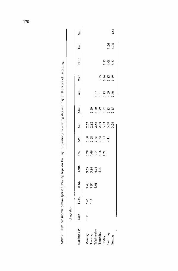
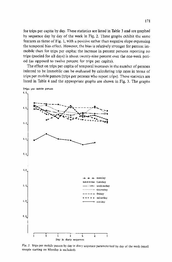
The effect on trips per capita of temporal increases in the number of persons inferred to be immobile can be evaluated by calculating trip rates in terms of trips per mobile person (trips per persons who report trips). These statistics are listed in Table 4 and the appropriate graphs are shown in Fig. 3. The graphs
Trips per mobile person
4.
4.C
3.C
2.
1.q
0.!
7..7- ~ . ~ - - - . ~
~ , + ~ ~ : : ~ - ~ : ~ s - ~ , - . - - = . , • X ' ~ , ~ : ~ . , - ~:~ '~. " - - -~
~ ~ m o n d a y
A _ _ z : ~ t u e s d a y
- - - ~ wednesday
............. thursday
. . . . . f r i d a y
~ + ÷ * s a t u r d a y
s u n d a y
i i m ~ l i n 1 2 3 5 6 7
Day in diary sequenee
Fig. 3. Trips per mobile person by day in diary sequence parameterised by day of the week (small sample starting on Monday is excluded).
172
exhibit a similar form to those of Fig. 1, but the level of bias is less: approxi- mately six percent over the period of seven days.
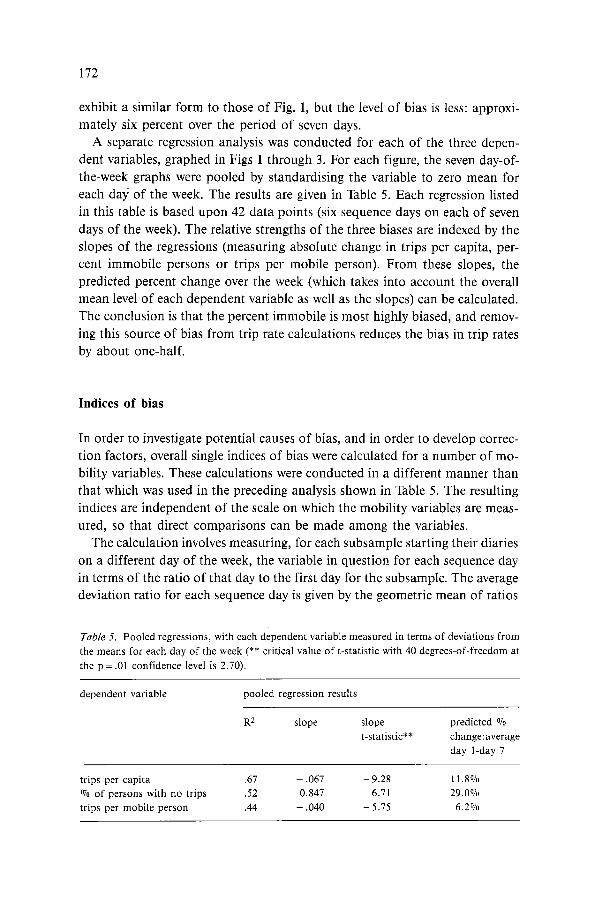
A separate regression analysis was conducted for each of the three depen- dent variables, graphed in Figs 1 through 3. For each figure, the seven day-of- the-week graphs were pooled by standardising the variable to zero mean for each da3/of the week. The results are given in Table 5. Each regression listed in this table is based upon 42 data points (six sequence days on each of seven days of the week). The relative strengths of the three biases are indexed by the slopes of the regressions (measuring absolute change in trips per capita, per- cent immobile persons or trips per mobile person). From these slopes, the predicted percent change over the week (which takes into account the overall mean level of each dependent variable as well as the slopes) can be calculated. The conclusion is that the percent immobile is most highly biased, and remov-
ing this source of bias from trip rate calculations reduces the bias in trip rates by about one-half.
Indices of bias
In order to investigate potential causes of bias, and in order to develop correc- tion factors, overall single indices of bias were calculated for a number of mo- bility variables. These calculations were conducted in a different manner than that which was used in the preceding analysis shown in Table 5. The resulting indices are independent of the scale on which the mobility variables are meas-
ured, so that direct comparisons can be made among the variables. The calculation involves measuring, for each subsample starting their diaries
on a different day of the week, the variable in question for each sequence day in terms of the ratio of that day to the first day for the subsample. The average deviation ratio for each sequence day is given by the geometric mean of ratios
Table 5. Pooled regressions, with each dependent variable measured in terms of deviations from
the means for each day of the week (** critical value of t-statistic with 40 degrees-of-freedom at
the p - . 0 1 confidence level is 2.70).
dependent variable pooled regression results
R 2 slope slope predicted % t-statistic** change:average
day 1-day 7
trips per capita .67 - . 0 6 7 - 9 . 2 8 11.8% % of persons with no trips .52 0.847 6.71 29.0% trips per mobile person .44 - . 0 4 0 - 5 . 7 5 6.2%
173
deviation r~tio
1.• index: slope: - .025/day
0.9 .964 • ~ - - - ~ , - . . _ ~ .925 .923 ~ o
0.8 .855 .877
0.7
0.6
O.
0.4.
0.3
0.2
day in diary sequence
0.
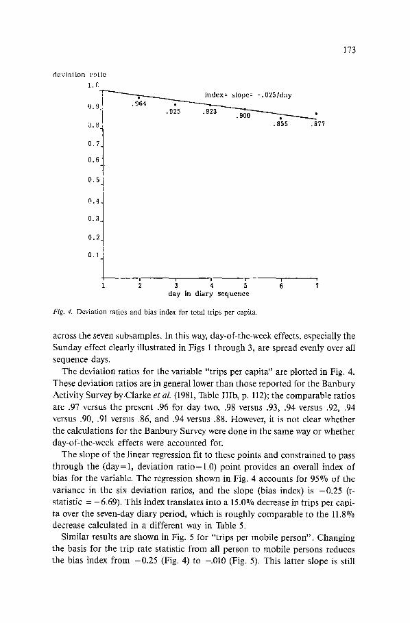
Fig. 4. Deviation ratios and bias index for total trips per capita.
across the seven subsamples. In this way, day-of-the-week effects, especially the Sunday effect clearly illustrated in Figs 1 through 3, are spread evenly over all sequence days.
The deviation ratios for the variable "trips per capita" are plotted in Fig. 4. These deviation ratios are in general lower than those reported for the Banbury Activity Survey by.Clarke et al. (1981, Table IIIb, p. 112); the comparable ratios are .97 versus the present .96 for day two, .98 versus .93, .94 versus .92, .94 versus .90, .91 versus .86, and .94 versus .88. However, it is not clear whether the calculations for the Banbury Survey were done in the same way or whether day-of-the-week effects were accounted for.
The slope of the linear regression fit to these points and constrained to pass through the (day= 1, deviation ratio= 1.0) point provides an overall index of bias for the variable. The regression shown in Fig. 4 accounts for 95% of the variance in the six deviation ratios, and the slope (bias index) is -0 .25 (t- statistic = -6.69). This index translates into a 15.0% decrease in trips per capi- ta over the seven-day diary period, which is roughly comparable to the 11.8% decrease calculated in a different way in Table 5.
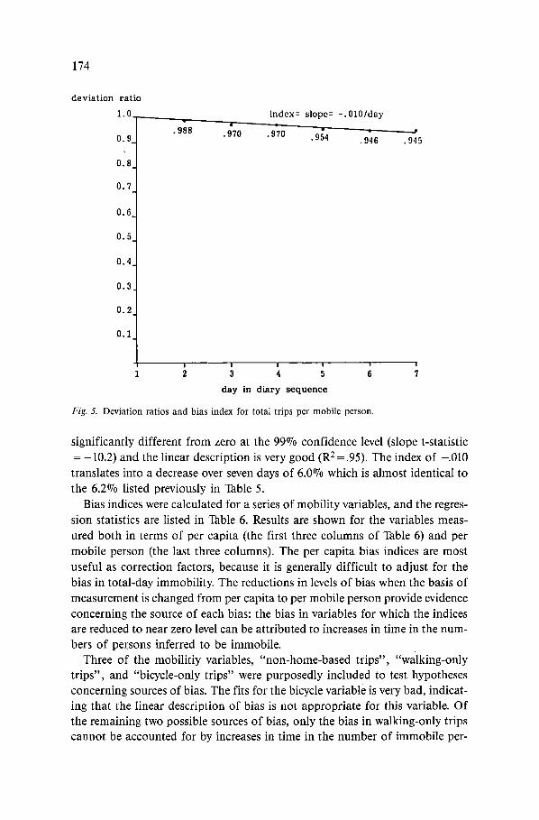
Similar results are shown in Fig. 5 for "trips per mobile person". Changing the basis for the trip rate statistic from all person to mobile persons reduces the bias index from -0.25 (Fig. 4) to -.010 (Fig. 5). This latter slope is still
174
d e v i a t i o n r a t i o
1 . 0 _ _
• 988 .970 0.9
0.8
0.7
0.6
0.5
0.4
0.3
0.2
0"1 t I I I ! !
1 2 3 4 5 6
day in diary sequence
Fig. 5. Deviation ratios and bias index for total trips per mobile pcrson.
index= slope= -•OlO/day
• 970 •9 ;4 .946 ,945
significantly different from zero at the 99% confidence level (slope t-statistic = -10.2) and the linear description is very good (R 2= .95). The index of -.010
translates into a decrease over seven days of 6.0% which is almost identical to the 6.2% listed previously in Table 5.
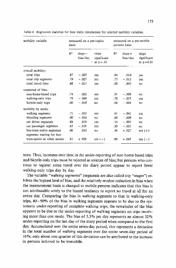
Bias indices were calculated for a series of mobility variables, and the regres- sion statistics are listed in Table 6. Results are shown for the variables meas- ured both in terms of per capita (the first three columns of Table 6) and per mobile person (the last three columns). The per capi ta bias indices are most
useful as correction factors, because it is generally difficult to adjust for the bias in total-day immobility. The reductions in levels of bias when the basis of
measurement is changed from per capita to per mobile person provide evidence concerning the source of each bias: the bias in variables for which the indices are reduced to near zero level can be attributed to increases in time in the num- bers of persons inferred to be immobile.
Three of the mobilitiy variables, "non-home-based trips", "walking-only trips", and "bicycle-only trips" were purposedly included to test hypotheses concerning sources of bias. The fits for the bicycle variable is very bad, indicat- ing that the linear description of bias is not appropriate for this variable. Of the remaining two possible sources of bias, only the bias in walking-only trips cannot be accounted for by increases in time in the number of immobile per-
175
Table 6. Regression statistics for bias index calculations for selected mobility variables,
mobility variable measured on a per-capita measured on a per-mobile basis persons basis
R 2 s lope = s lope R 2 s lope = s lope
b i a s / d a y s ignif icant b i a s / d a y s ignif icant
- at p = . 0 1 at p = 0 . 0 1
overall mobility: total trips .87 -.025 yes .94 -.010 yes total trip segments .79 -.027 yes .75 -.012 yes total travel time .68 -.013 yes .00 + .003 no
suspected of bias: non-home-based trips .74 -.022 yes .31 -.008 no walking-only trips .78 -.048 yes .70 -.035 yes bicycle-only trips .00 -,019 no .00 -.004 no
mobility by mode: walking segments .71 -.053 yes .61 -.041 yes bicycling segments .00 -.024 no .00 -.009 no car driver segments .88 -.019 yes .14 -.005 no car passenger segments .85 - .018 yes .30 - .003 no bus-tram-metro segments .06 - .010 no .36 + .027 yes ( + ) segments waiting for bus- tram-metro or other modes .81 + .028 yes (+) .90 + .045 yes (+)
sons. Thus, increases over time in the under-repor t ing of non-home-based trips
and bicycle-only trips must be rejected as sources of bias; but persons who con-
t inue to register some travel over the diary period appear to report fewer
walking-only trips day by day.
The variable "walking segments" (segments are also called trip "stages") ex-
hibits the highest level of bias, and the relatively modest reduct ion in bias when
the measurement basis is changed to mobile persons indicates that this bias is
not a t t r ibutable solely to the biased tendancy to report no travel at all for an
entire day. Compar ing the bias in walking segments to that in walking-only
trips, 8 0 - 9 0 % of the bias in walking segments appears to be due to the sys-
tematic under- repor t ing of complete walking trips; the remainder of the bias
appears to be due to the under-repor t ing of walking segments on trips involv-
ing more t han one mode. The bias of 5.3% per day represents an almost 32%
under- repor t ing on the last day of the diary period when compared to the first
day. Accumula ted over the entire seven-day period, this represents a deviat ion
in the total n u m b e r of walking segments over the entire seven-day period of
16%; only about one-quar ter of this deviat ion can be at t r ibuted to the increase
in persons inferred to be immobile.
176
The two overall mobility variables "total trips" and "total trip segments" both exhibit bias levels which cannot be accounted for by increases in the num- ber of immobile persons. The biases for trips and trip segments are approxi- mately equal, which indicates that entire trips, rather than trip components, are subject to bias. However, the biases in trip segments by car driver and car passenger modes can largely be explained by the numbers of immobile persons. Thus, it appears that people, who continue to report each day's travel, tend to overlook short, non-vehicular trips with increasing incidence during the diary period. The emphasis on short trips is shown by the negligable bias in total travel time per mobile person.
Different results are found for "bus-tram-metro trip segments" and "waiting segments". Both of these variables exhibit posi t ive biases when measured on a per-mobile-person basis. In addition, waiting segments are positively biased on a per-capita basis as well. There appears to be a positive learning effect for these variables: reporting is improved day by day for persons reporting any travel at all.
Differences in biases over population segments
Many of the important questions in travel behaviour research involve compari- sons over population segments. The temporal biases identified in Table 6 would only affect the answers to such questions if population segments differed in terms of the levels of bias in their responses. In the final stage of the present analysis, tests were conducted in order to detect any such differ- ences in bias levels. Segmentation differences were investigated using the meth- od of multivariate analysis of variance with repeated-measurements designs (or, repeated-measurements MANOVA). These analyses were at a disaggregate level, with the sample size for each test being the total number of 3,863 respon- dents (minus the 59 respondents who were immobile on all seven days and the small subsample of 34 respondents beginning their diaries on Monday). The methodology of repeated-measurements MANOVA is described in detail in Winer (1971, Chapter 6) and Bock (1975, Chapter 7).
A separate MANOVA was conducted for each of the mobility variables list- ed in Table 6 and for each of eight population segmentations described in Ta-
ble 7. In each MANOVA, the dependent variables were the measurements of the
mobility variable in question on each of the diary sequence days; the between- subjects independent factors were the starting day of the Week and the segmen- tation variable; and the within-subjects factors were the sequence days.
The MANOVA designs accounted first for the main effect of starting day of the week (a six-category variable), the main effect of the segmentation varia-
177
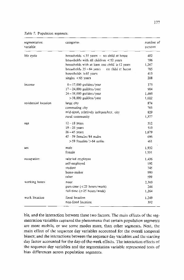
Table 7. Population segments.
segmentation categories number of variable persons
life cycle households < 35 years - no child at home 402 households with all children < 12 years 786 households with at least one child >_ 12 years 1,267 households 35- 64 years - no child at home 785 households >-65 years 415 singles <65 years 208
income O- 17,000 guilders/year 375 17 - 24,000 guilders/year 904 24 - 38,000 guilders/year 1,460
> 38,000 guilders/year 1,022
residential location large city 874 commuting city 783 mid-sized, relatively independent, city 829 rural community 1,377
age 12- 18 years 512 19- 25 years 510 26 - 45 years 1,679 45 - 59 females/64 males 696
> 59 females/> 64 males 461
sex male 1,932 female 1,931
occupation salaried employee 1,436 self-employed 102 student 745 home-maker 980 other 599
working hours none 2,303 part-time (< 25 hours/week) 244 full-time (>_25 hours/week) 1,264
work location fixed location 1,249 non-fixed location 302
ble, a n d the i n t e r a c t i o n b e t w e e n these two factors . T h e m a i n effects o f the seg-
m e n t a t i o n var iab les c a p t u r e d the p h e n o m e n a tha t ce r t a in p o p u l a t i o n s egmen t s
are m o r e mobi le , o r use s o m e m o d e s more , t h a n o t h e r segments . Next , the
m a i n e f fec t o f the s e q u e n c e day var iab les a c c o u n t e d for the overal l t e m p o r a l
biases; and the i n t e r ac t ions b e t w e e n the s e q u e n c e day var iab les a n d the s ta r t ing
day fac to r a c c o u n t e d for t he day -o f - the -week effects . T h e i n t e r ac t i on effects o f
t he s e q u e n c e day var iab les a n d the s e g m e n t a t i o n va r i ab le r ep resen ted tests o f
bias d i f fe rences across p o p u l a t i o n segments .
178
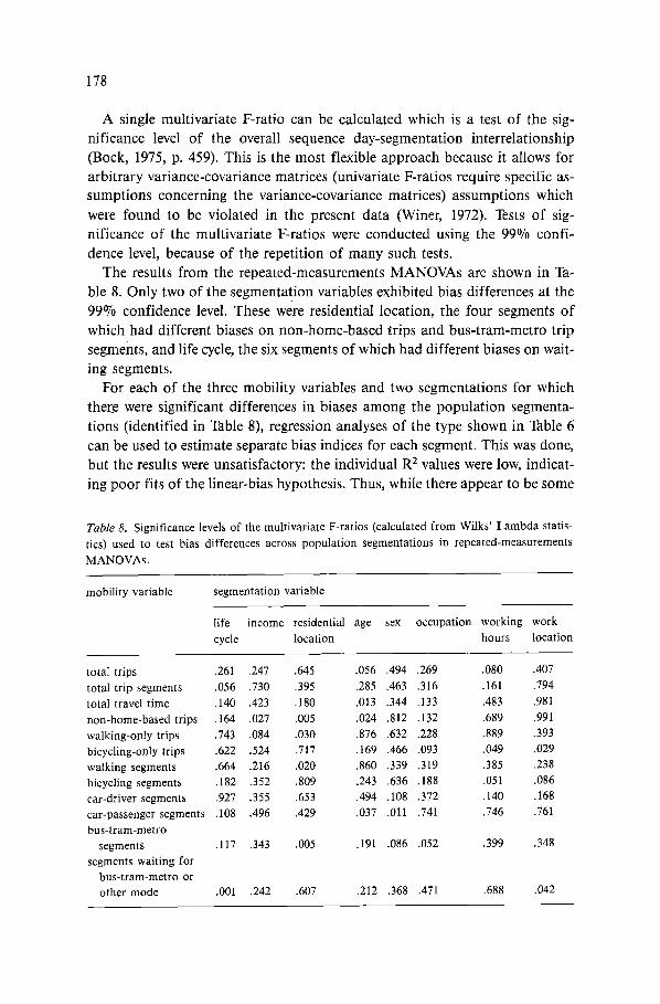
A single multivariate F-ratio can be calculated which is a test of the sig- nificance level of the overall sequence day-segmentation interrelationship (Bock, 1975, p. 459). This is the most flexible approach because it allows for arbitrary variance-covariance matrices (univariate F-ratios require specific as- sumptions concerning the variance-covariance matrices) assumptions which
were found to be violated in the present data (Winer, 1972). Tests of sig- nificance of the multivariate F-ratios were conducted using the 99% confi- dence level, because of the repetition of many such tests.
The results from the repeated-measurements MANOVAs are shown in Ta- ble 8. Only two of the segmentation variables exhibited bias differences at the 99% confidence level. These were residential location, the four segments of which had different biases on non-home-based trips and bus-tram-metro trip segments, and life cycle, the six segments of which had different biases on wait- ing segments.
For each of the three mobility variables and two segmentations for which there were significant differences in biases among the population segmenta- tions (identified in Table 8), regression analyses of the type shown in Table 6 can be used to estimate separate bias indices for each segment. This was done, but the results were unsatisfactory: the individual R 2 values were low, indicat-
ing poor fits of the linear-bias hypothesis. Thus, while there appear to be some
Table 8. Significance levels of the multivariate F-ratios (calculated from Wilks' Lambda statis-
tics) used to test bias differences across population segmentations in repeated-measurements
MANOVAs.
mobility variable segmentation variable
life income residential age sex occupation working work
cycle location hours location
total trips .261 .247 .645
total trip segments .056 .730 .395
total travel time .140 .423 .180
non-home-based trips .164 .027 .005
walking-only trips .743 .084 .030
bicycling-only trips .622 .524 .717 walking segments .664 .216 .020
bicycling segments .182 .352 .809 car-driver segments .927 .355 .653
car-passenger segments .108 .496 .429
bus- t ram-metro segments .117 .343 .005
segments waiting for bus- t ram-metro or other mode .001 .242 .607
.056 .494 .269 .080 .407
,285 .463 .316 .161 .794
.013 .344 .133 .483 ,981
.024 .812 .132 ~689 .991
.876 .632 .228 .889 .393
.169 .466 .093 .049 .029
.860 .339 .319 .385 .238
.243 .636 .188 .051 .086
.494 .108 .372 .140 .168
.037 .011 .741 .746 .761
.191 .086 .052 ,399 .348
.212 .368 .471 .688 .042
179
differences among the segments, these differences are not readily explained in the same manner as for the total population. It is possible that a larger sample
is needed to pursue these analyses.
Conclusions
It is concluded that there are indeed temporal biases in multi-day travel diaries. The diary instrument of the 1984 Dutch National Mobility Panel is judged to be representative of modern diary instruments; experiences from other surveys were drawn upon in developing an instrument which respondents would find easy to use and interesting. Yet these diary data were found to be clearly biased. Moreover, the levels of these biases are sufficient as to be important even in
diaries of only two or three days. The principal cause of these temporal biases is the increasing tendancy over
time for respondents to report no travel at all on a given day. In the present dataset, there was an approximately 4.8% per day increase in the number of respondents inferred to be immobile for an entire day. This trend substantially explains the temporal biases in many mobility variables which are measured on a per capita (or per household) basis: total daily travel time, the number of non-home-based trips, and car-driver and car-passenger trip segments (seg- ments are also called trip stages, or, in the case of vehicular modes, rides).
Efforts must be made in future travel surveys to discourage respondents from deleting entire days from their diaries. Possibly interviewers could check on this item in surveys which include pick-up of the diaries at respondents' homes, or telephone contacts could be used in survey using postal returns. It might also be possible that diaries specifically designed to increase the repor- ing of short trips and obtain more detailed descriptions of activities result in greater biases in non-reporting of entire days because of increased respondent fatigue. That is, a more complete diary might lead to more days of inferred im-
mobility. However, certain temporal biases cannot be explained by increases over time
in the number of respondents inferred to be immobile. Most importantly, there is a day-to-day increase in the under-reporting of short walking trips. The rate of decrease in walking-only trips per mobile person was 3.5% per day in the present dataset. This appears to be the main source of the bias in total trips per day per mobile person, a statistic which decreases at the rate of about 1.0% per day over the diary period.
The remaining biases are more complex. Walking segments are increasingly under-reported even after accounting for the bias in walking-only trips. And there are opposite effects in the reporting of trip segments by tram-bus-metro and waiting: bus-tram-metro segments per mobile person increases at a rate of
180
2.7% per day, and waiting segments per mobile person increases at a rate of
4.5% per day. There is apparently a learning effect involved in the reporting of the waiting time and transfers involved in use of bus-tram-metro services. These counter-acting effects involving walking and bus-tram-metro result in an
overall bias in total trip segments per mobile person which is only slightly greater than the bias in total trips per mobile person.
There was a failure to identify differences in levels of bias across population
segments. This result has both a positive and negative interpretation for travel behaviour modelling: Positively, it can be expected that temporal biases will not significantly affect behavioural comparisons among population segments. Negatively, it will be more difficult to trace the sources of the biases when such
biases cannot be linked to respondent socio-demographic characteristics. And
the accuracy of correction factors cannot readily be improved by disaggregat- ing such factors by segment.
It is recommended that correction factors be applied tO multi-day diary data
in order to adjust data from later days to the level of data from the first day. One such set of correction factors is represented by the six mode-specific "seg- ments per capita" bias indices listed in the last six rows of Table 6, plus the
index for "total trip segments per capita" for modes for which insufficient data was available for separate calculations. These indices, ranging from -.053 (a decrease of 5.3°7o per day) for walking segments to +.028 (an increase of 2.8%
per day) for waiting segments, can be applied to all diary data categorised by mode and diary sequence day. The concept of a "main mode", defined either
by travel time or travel distance, can be used to weight data concerning trip purposes, times of day, etc.
These corrections can be accomplished analogously to the way in which weights for persons and households are applied on the basis of sociodemo-
graphic characteristics (a process usually called "expansion of the sample"). Most statistical-analysis computer packages have automatic procedures for ap- plying such weights in statistical computations. Tests of the effects of the cor- rection factors on the results of various travel behaviour analyses can be ascer-
taind by repeating the analyses with and without the application of the weights. This remains a subject for further research.
References
Bock, R.D., 1975. Multivariate Statistical Methods in Behavioral Research. New York: McGraw-Hill.
Br6g, W. & E. Ampt, 1982. State of the Art in the Collection of Travel Behavior Data. In Special Report 201: Travel Analysis Methods for the 1980s. Washington, D.C.: National Research Council.
Br6g, W. & A. H. Meyburg, 1980. The Non-Response Problem in Travel Surveys: An Empirical Investigation. Transportation Research Record No. 775, pp. 34-38.
181
Br6g, W. & A. H. Meyburg, 1981. Consideration of Non-Response Effects in Large-Scale Mobil- ity Surveys. Transportation Research Record No. 807, pp. 39-46.
Clarke, M., M. Dix & P. Jones, 1981. Error and Uncertainty in Travel Surveys. Transportation, 10: pp. 105-126.
Goodwin, P.B., 1979. The Usefulness of Travel Budgets. Transportation Research, 15A: pp. 71- 80.
Hanson, S. & J. O. Huff, 1981. Assessing Day-to-Day Variability in Complex Travel Patterns. Transportation Research Record No. 891: pp. 18-2&
Van der Hoorn, T., 1979. Travel Behaviour and the Total Activity Pattern. Tranportation, 8: pp. 309-328.
Jones, P. M., M. Dix, M. C. Clarke & I. G. Heggie, 1980. Understanding. Travel Behaviour. Transport Studies Unit, University of Oxford. Project Report llglPR.
Koppelman, F. S. & E. I. Pas, 1984. Estimation of Disaggregate Regression Models of Person Trip Generation with Multiday Data. In J. Volmuller and R. Hamerslag, eds., Proceedings of the Ninth International Symposium on Transportation and Traffic Theory, pp. 513-532. Utrecht: VNU Science Press.
Lyn, A. & J. Ruchon, 1979. Exposure to the Risk of an Accident: A Description of the Data Collection and Processing Procedures, Analysis of their Effectiveness. Canadian Facts, Toronto.
Scheuch, E. K., 1972. The Time-Budget Interview. In A. Szalai, ed., The Use of Time. The Hague: Mouton Press.
Szalai, A., 1972. Design Specifications for the Surveys. In A. Szalai, ed., The Use of Time. The Hague: Mouton Press.
Wirier, B. J., 1971. Statistical Principles in Experimental Design, 2d ed. New York: McGraw-Hill.