Embed Size (px)
DESCRIPTION
Bicriteria Robustness versus Cost Optimisation in the Generation of Aircrew Pairings. David M Ryan and Matthias Ehrgott Department of Engineering Science University of Auckland {d.ryan,m.ehrgott}@auckland.ac.nz. The University of Auckland. - PowerPoint PPT Presentation
Citation preview
TheUniversity
of Auckland
IMA WorkshopUniversity of Auckland
New ZealandOperations Research GroupDepartment of Engineering Science
TheUniversity
of Auckland
Bicriteria Robustness versus Cost Optimisation
in the Generation of Aircrew Pairings David M Ryan and Matthias Ehrgott
Department of Engineering ScienceUniversity of Auckland
{d.ryan,m.ehrgott}@auckland.ac.nz
Part 1: The Tour of Duty (ToD) problem of aircrew scheduling Model, properties, computation, resultsMinimum cost maximum potential disaster
Part 2: Non-robustness – the consequences of minimum costA non-robustness measureThe min cost / max robustness ToD problem
Operations Research GroupDepartment of Engineering Science
2
The University of AucklandNew ZealandIMA Workshop
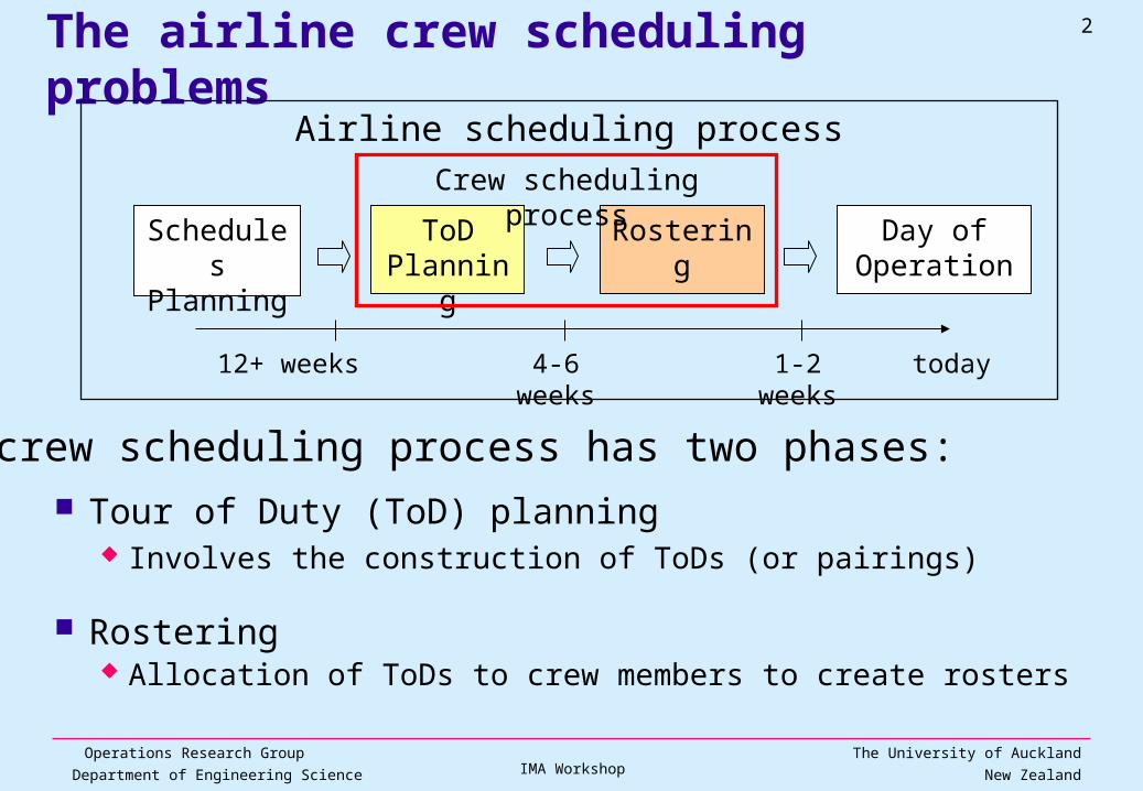
The airline crew scheduling problems
Tour of Duty (ToD) planning Involves the construction of ToDs (or pairings)
Rostering Allocation of ToDs to crew members to create rosters
Airline scheduling process
Schedules Planning
ToDPlanning
Rostering Day of Operation
today12+ weeks 4-6 weeks 1-2 weeks
Crew scheduling process
The crew scheduling process has two phases:
Operations Research GroupDepartment of Engineering Science
3
The University of AucklandNew ZealandIMA Workshop
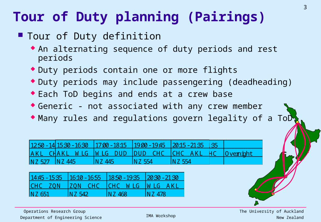
Tour of Duty planning (Pairings) Tour of Duty definition
An alternating sequence of duty periods and rest periods Duty periods contain one or more flights Duty periods may include passengering (deadheading) Each ToD begins and ends at a crew base Generic - not associated with any crew member Many rules and regulations govern legality of a ToD
12:50 - 14:10 14:45 - 15:35 16:10 - 16:55 18:25 - 19:45 20:15 - 21:35AKL CHC CHC ZQN ZQN CHC CHC AKL AKL CHC OvernightNZ 527 NZ 651 NZ 542 NZ 548 NZ 559
14:45 - 15:35 16:10 - 16:55 18:50 - 19:35 20:30 - 21:30CHC ZQN ZQN CHC CHC WLG WLG AKLNZ 651 NZ 542 NZ 468 NZ 478
15:30 - 16:30 17:00 - 18:15 19:00 - 19:45 20:15 - 21:35AKL WLG WLG DUD DUD CHC CHC AKLNZ 445 NZ 445 NZ 554 NZ 554
Operations Research GroupDepartment of Engineering Science
4
The University of AucklandNew ZealandIMA Workshop
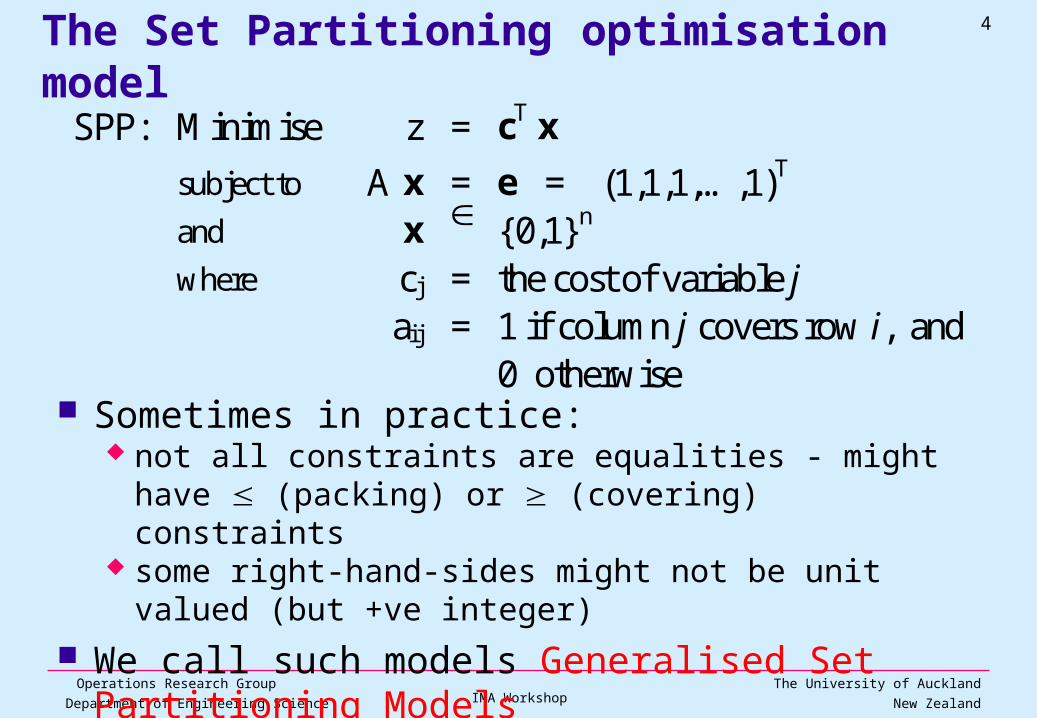
The Set Partitioning optimisation model
SPP: Minimise z = cT x
subject to A x = e = (1,1,1,…,1)T and x {0,1}n where cj = the cost of variable j aij = 1 if column j covers row i, and 0 otherwise
Sometimes in practice: not all constraints are equalities - might have (packing) or
(covering) constraints some right-hand-sides might not be unit valued (but +ve integer)
We call such models Generalised Set Partitioning Models Special forms of GSPP for ToD planning (and Rostering)
Operations Research GroupDepartment of Engineering Science
5
The University of AucklandNew ZealandIMA Workshop
1
2
53
4
6
7
A
B
A
B
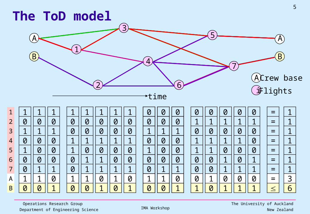
The ToD model
011001001
010011001
011101001
101101001
101001001
100011010
101100010
101001010
101101010
010011010
========
631111111
011000101
101000101
010010101
B
A
7
6
5
4
3
2
1
010010100
011000100
101000100
i Flights
A Crew base
time
Operations Research GroupDepartment of Engineering Science
6
The University of AucklandNew ZealandIMA Workshop
The Tour of Duty SPP model Rows (constraints) correspond to flights
Over one day or one week or some specified time period Also have base constraints
limit number of ToDs or total ToD hours at a base
Columns (variables) represent feasible ToDs Each column must satisfy many rules (constraints) which are
implicitly represented
Up to 2000 constraints (m), many millions (or billions!!) of variables (n)
The objective is to minimise the total dollar cost Costs include allowances, hotel and meal costs, ground transport
costs, passengering costs, paid duty hours The cost of each legal ToD can be calculated
Operations Research GroupDepartment of Engineering Science
7
The University of AucklandNew ZealandIMA Workshop
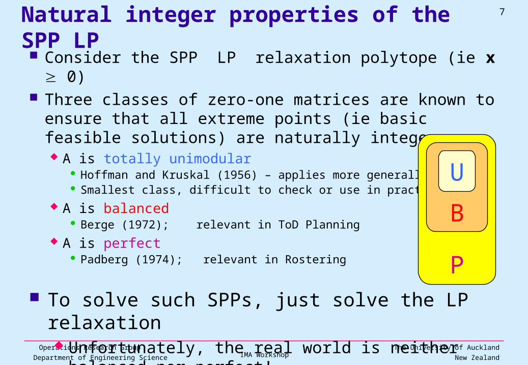
Natural integer properties of the SPP LP Consider the SPP LP relaxation polytope (ie x 0) Three classes of zero-one matrices are known to ensure that all
extreme points (ie basic feasible solutions) are naturally integer A is totally unimodular
Hoffman and Kruskal (1956) – applies more generally Smallest class, difficult to check or use in practice
A is balanced Berge (1972); relevant in ToD Planning
A is perfect Padberg (1974); relevant in Rostering P
B
U
To solve such SPPs, just solve the LP relaxation Unfortunately, the real world is neither balanced nor perfect!
Operations Research GroupDepartment of Engineering Science
8
The University of AucklandNew ZealandIMA Workshop
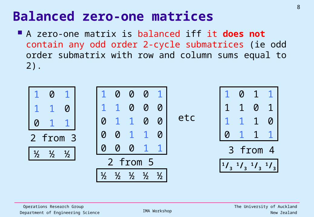
Balanced zero-one matrices A zero-one matrix is balanced iff it does not contain any
odd order 2-cycle submatrices (ie odd order submatrix with row and column sums equal to 2).
110
011
101
2 from 3
½½½11000
01100
00110
00011
10001
2 from 5
etc
½½½½½
1110
0111
1011
1101
3 from 41/3
1/31/3
1/3
Operations Research GroupDepartment of Engineering Science
9
The University of AucklandNew ZealandIMA Workshop
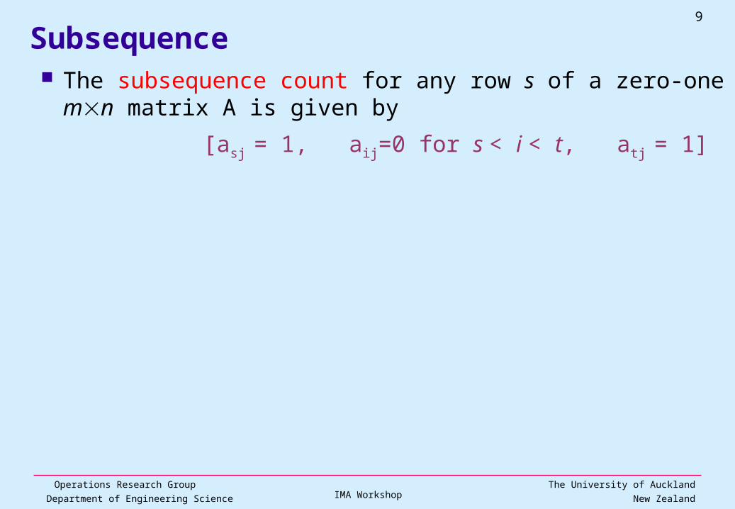
Subsequence The subsequence count for any row s of a zero-one mn
matrix A is given by
[asj = 1, aij=0 for s < i < t, atj = 1]
Operations Research GroupDepartment of Engineering Science
10
The University of AucklandNew ZealandIMA Workshop
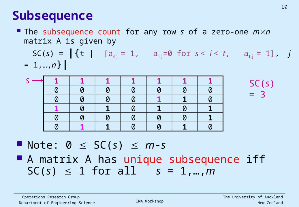
Subsequence The subsequence count for any row s of a zero-one mn matrix
A is given by
SC(s) = |{t | [asj = 1, aij=0 for s < i < t, atj = 1], j = 1,…,n}|
Note: 0 SC(s) m-s A matrix A has unique subsequence iff SC(s) 1 for all
s = 1,…,m
101001
000001
010101000010101011000000011111s SC(s) = 3
Operations Research GroupDepartment of Engineering Science
11
The University of AucklandNew ZealandIMA Workshop
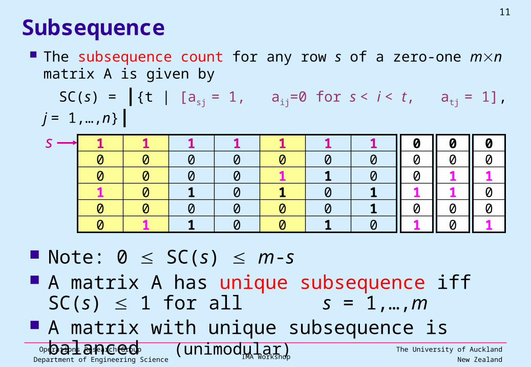
Subsequence The subsequence count for any row s of a zero-one mn
matrix A is given by
SC(s) = |{t | [asj = 1, aij=0 for s < i < t, atj = 1], j = 1,…,n}|
Note: 0 SC(s) m-s A matrix A has unique subsequence iff SC(s) 1 for all
s = 1,…,m A matrix with unique subsequence is balanced (unimodular)
101001
000001
010101000010101011000000011111s
101000
100100
001100
Operations Research GroupDepartment of Engineering Science
12
The University of AucklandNew ZealandIMA Workshop
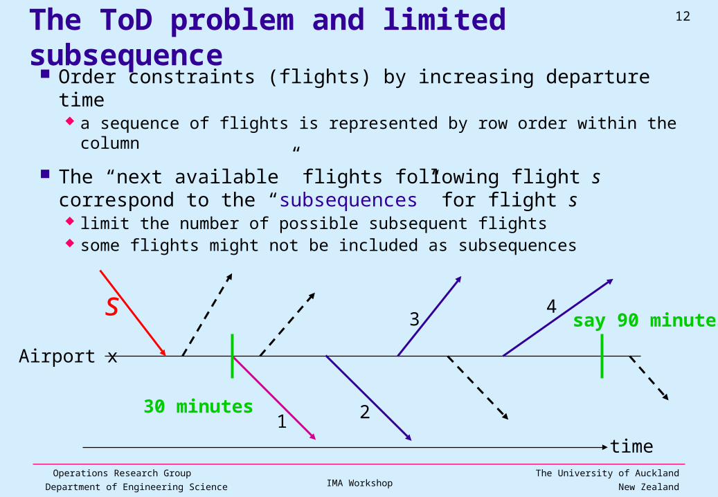
The ToD problem and limited subsequence Order constraints (flights) by increasing departure time
a sequence of flights is represented by row order within the column
The “next available” flights following flight s correspond to the “subsequences” for flight s limit the number of possible subsequent flights some flights might not be included as subsequences
s
2
34
1time
Airport x
30 minutes
say 90 minutes
Operations Research GroupDepartment of Engineering Science
13
The University of AucklandNew ZealandIMA Workshop
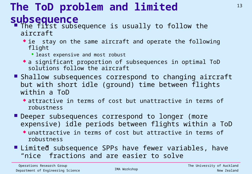
The ToD problem and limited subsequence The first subsequence is usually to follow the aircraft
ie stay on the same aircraft and operate the following flight least expensive and most robust
a significant proportion of subsequences in optimal ToD solutions follow the aircraft
Shallow subsequences correspond to changing aircraft but with short idle (ground) time between flights within a ToD attractive in terms of cost but unattractive in terms of robustness
Deeper subsequences correspond to longer (more expensive) idle periods between flights within a ToD unattractive in terms of cost but attractive in terms of robustness
Limited subsequence SPPs have fewer variables, have “nice” fractions and are easier to solve
Operations Research GroupDepartment of Engineering Science
14
The University of AucklandNew ZealandIMA Workshop
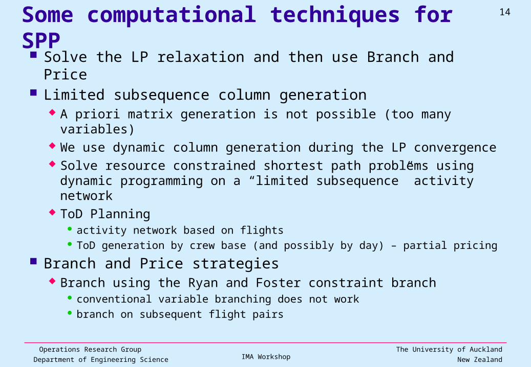
Some computational techniques for SPP Solve the LP relaxation and then use Branch and Price Limited subsequence column generation
A priori matrix generation is not possible (too many variables) We use dynamic column generation during the LP convergence Solve resource constrained shortest path problems using dynamic
programming on a “limited subsequence” activity network ToD Planning
activity network based on flights ToD generation by crew base (and possibly by day) – partial pricing
Branch and Price strategies Branch using the Ryan and Foster constraint branch
conventional variable branching does not work branch on subsequent flight pairs
Operations Research GroupDepartment of Engineering Science
15
The University of AucklandNew ZealandIMA Workshop
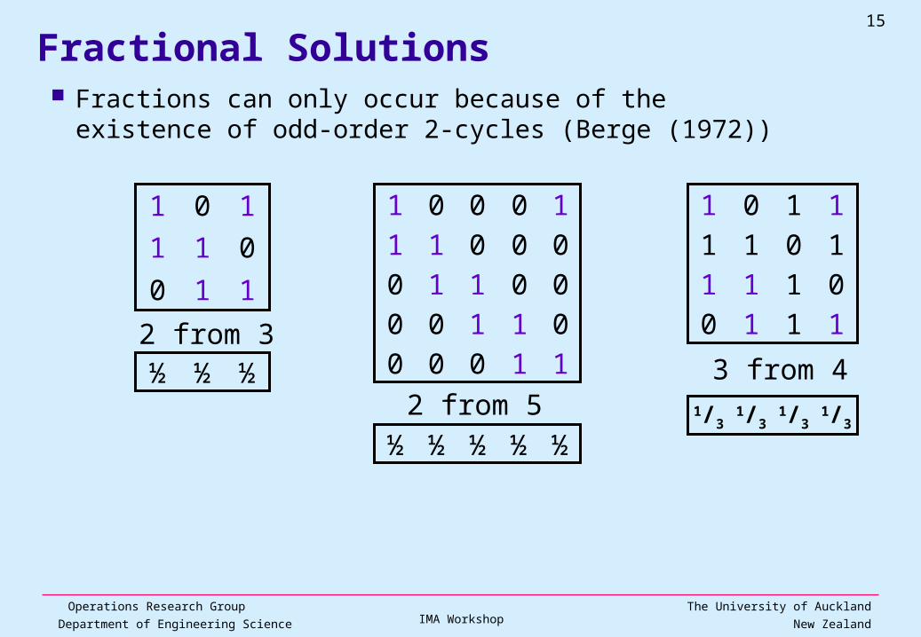
Fractions can only occur because of the existence of odd-order 2-cycles (Berge (1972))
Fractional Solutions
110
011
101
2 from 3½½½ 11000
01100
00110
00011
10001
2 from 5
½½½½½
1110
0111
1011
1101
3 from 41/3
1/31/3
1/3
Operations Research GroupDepartment of Engineering Science
16
The University of AucklandNew ZealandIMA Workshop
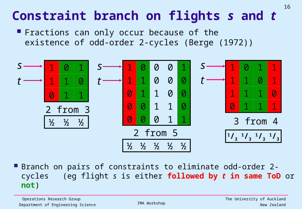
Fractions can only occur because of the existence of odd-order 2-cycles (Berge (1972))
Constraint branch on flights s and t
Branch on pairs of constraints to eliminate odd-order 2-cycles (eg flight s is either followed by t in same ToD or not)
s
t110
011
101
2 from 3½½½
ts
11000
01100
00110
00011
10001
2 from 5
½½½½½
1110
0111
1011
1101
3 from 41/3
1/31/3
1/3
st
Operations Research GroupDepartment of Engineering Science
17
The University of AucklandNew ZealandIMA Workshop
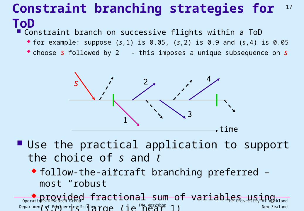
Constraint branching strategies for ToD Constraint branch on successive flights within a ToD
for example: suppose (s,1) is 0.05, (s,2) is 0.9 and (s,4) is 0.05 choose s followed by 2 - this imposes a unique subsequence on s
Use the practical application to support the choice of s and t follow-the-aircraft branching preferred – most “robust” provided fractional sum of variables using (s,t) is large (ie near 1) avoid (s,t) pairs involving aircraft change and short ground time
s 2
3
4
1time
Operations Research GroupDepartment of Engineering Science
18
The University of AucklandNew ZealandIMA Workshop
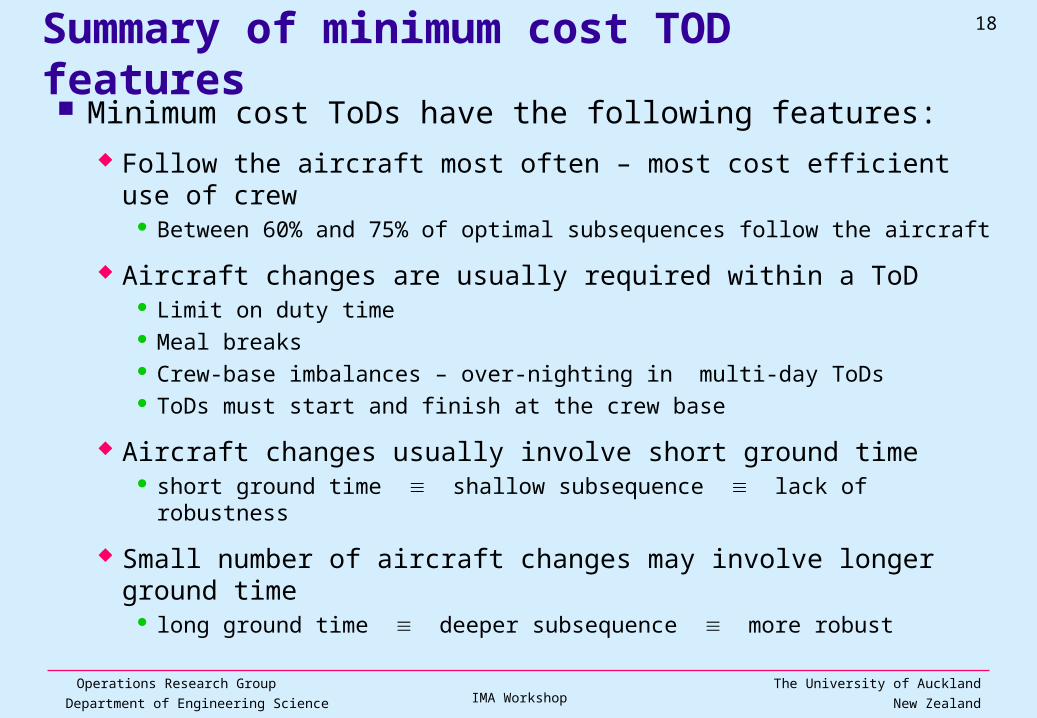
Summary of minimum cost TOD features Minimum cost ToDs have the following features:
Follow the aircraft most often – most cost efficient use of crew Between 60% and 75% of optimal subsequences follow the aircraft
Aircraft changes are usually required within a ToD Limit on duty time Meal breaks Crew-base imbalances – over-nighting in multi-day ToDs ToDs must start and finish at the crew base
Aircraft changes usually involve short ground time short ground time shallow subsequence lack of robustness
Small number of aircraft changes may involve longer ground time long ground time deeper subsequence more robust
Operations Research GroupDepartment of Engineering Science
19
The University of AucklandNew ZealandIMA Workshop
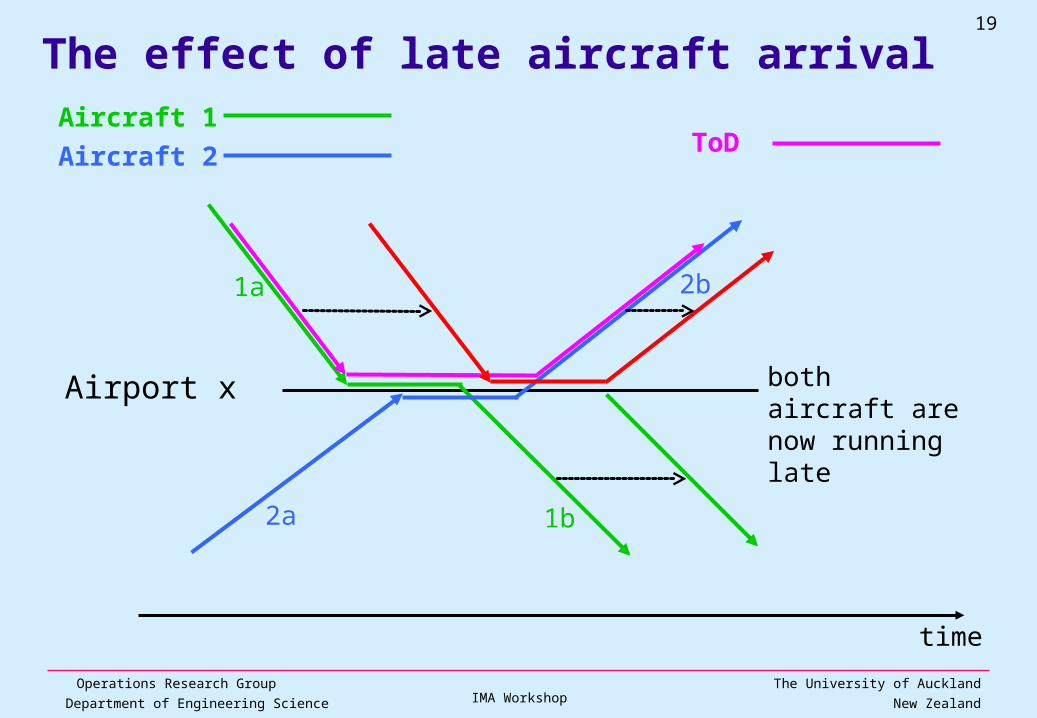
The effect of late aircraft arrival
Airport x
time
1b
1a
Aircraft 1
2b
2a
Aircraft 2 ToD
both aircraft are now running late
Operations Research GroupDepartment of Engineering Science
20
The University of AucklandNew ZealandIMA Workshop
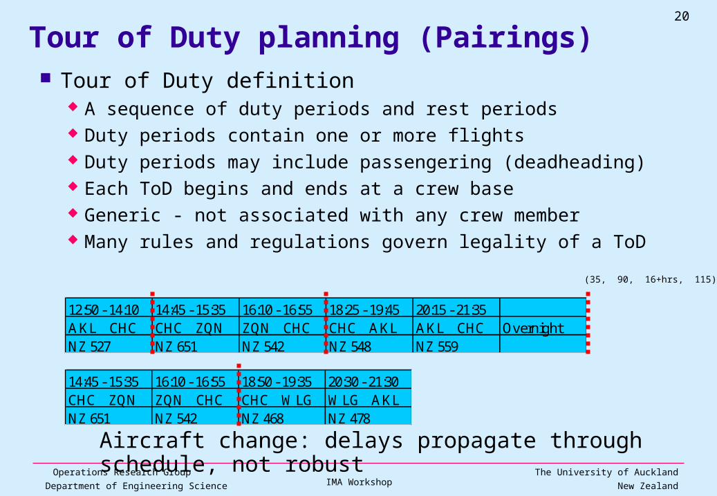
Tour of Duty planning (Pairings) Tour of Duty definition
A sequence of duty periods and rest periods Duty periods contain one or more flights Duty periods may include passengering (deadheading) Each ToD begins and ends at a crew base Generic - not associated with any crew member Many rules and regulations govern legality of a ToD
12:50 - 14:10 14:45 - 15:35 16:10 - 16:55 18:25 - 19:45 20:15 - 21:35AKL CHC CHC ZQN ZQN CHC CHC AKL AKL CHC OvernightNZ 527 NZ 651 NZ 542 NZ 548 NZ 559
14:45 - 15:35 16:10 - 16:55 18:50 - 19:35 20:30 - 21:30CHC ZQN ZQN CHC CHC WLG WLG AKLNZ 651 NZ 542 NZ 468 NZ 478
Aircraft change: delays propagate through schedule, not robust
(35, 90, 16+hrs, 115)
Operations Research GroupDepartment of Engineering Science
21
The University of AucklandNew ZealandIMA Workshop
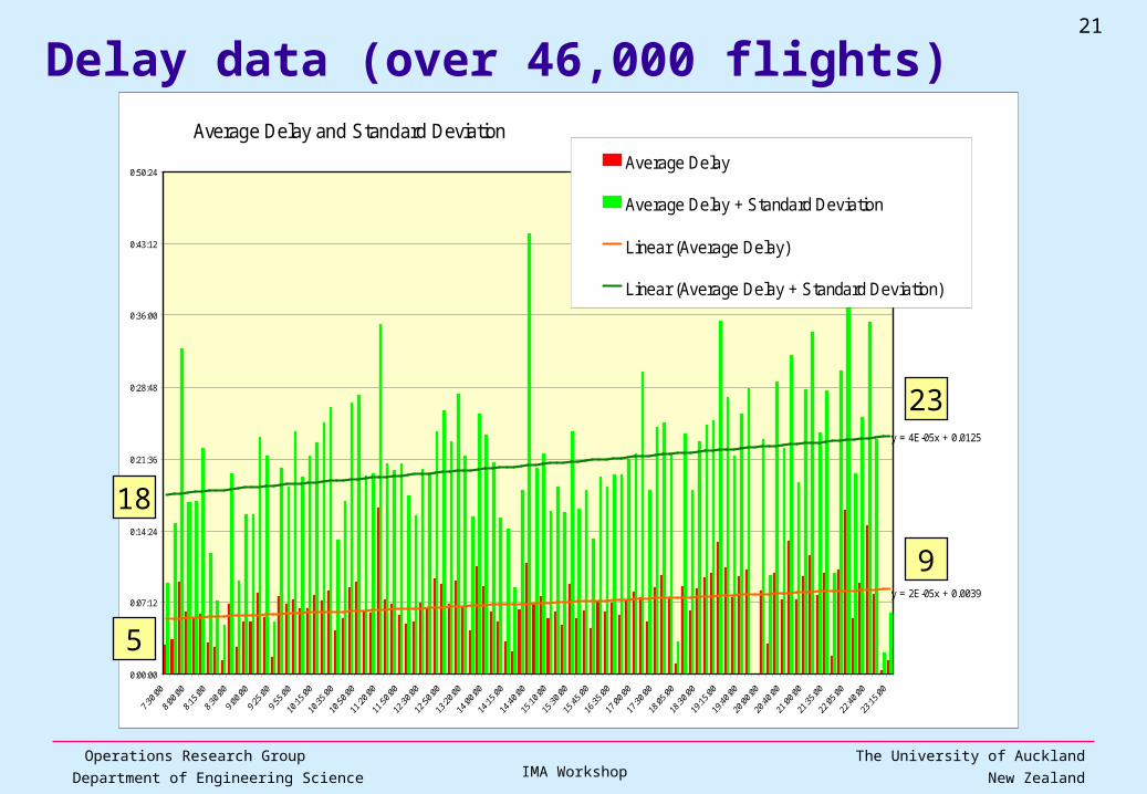
Delay data (over 46,000 flights) Average Delay and Standard Deviation
y = 2E-05x + 0.0039
y = 4E-05x + 0.0125
0:00:00
0:07:12
0:14:24
0:21:36
0:28:48
0:36:00
0:43:12
0:50:24Average Delay
Average Delay + Standard Deviation
Linear (Average Delay)
Linear (Average Delay + Standard Deviation)
5
9
23
18
Operations Research GroupDepartment of Engineering Science
22
The University of AucklandNew ZealandIMA Workshop
How can we introduce robustness into ToD build? Yen and Birge - A Stochastic Programming Approach to the
Airline Crew Scheduling Problem Formulate the ToD problem as a two-stage stochastic binary
optimisation problem with recourse: the first stage is based on the GSPP formulation
The recourse problem measures cost of delays evaluation requires solution of one LP for each scenario determines a so-called “switching cost” associated with aircraft change “switching cost” is used to remove expensive aircraft changes in next GSPP
The results show: small decrease in number of aircraft changes longer ground time when changing aircraft within a ToD
A rather computationally expensive means of treating the problem requires repeated solution of the deterministic GSPP
Operations Research GroupDepartment of Engineering Science
23
The University of AucklandNew ZealandIMA Workshop
How can we introduce robustness into ToD build? Schaefer, Johnson, Kleywegt and Nemhauser –
Airline Crew Scheduling under Uncertainty Use an “operational cost” instead of a “planned cost” for each ToD Monte Carlo simulation to estimate “operational cost” The simulation (using SimAir) focuses on one ToD at a time and
ignores the interactive effects between ToDs Schaefer et al suggest that this approach can be shown to account for
approximately 90% of the total disruption costs
This approach is not compatible with column generation since the “operational cost” is only available after simulation
Penalizes ToDs with expensive “operational cost” The observed effect of this approach is to produce ToDs with
lower operational cost than those produced with planned cost
Operations Research GroupDepartment of Engineering Science
24
The University of AucklandNew ZealandIMA Workshop
How can we introduce robustness into ToD build? Our approach is to develop a measure of “non-robustness”
for each ToD based on the effect of potential delays within the ToD If the ToD stays with the aircraft there will be no penalty If the ToD changes aircraft, the penalty will reflect the potential
disruption effect of the possible delay at the aircraft change Ignore the interactive effects between ToDs
Then treat the non-robustness measure as a second objective The “non-robustness” objective measure should be additive across
the ToD So it is compatible with column generation solution procedures
Operations Research GroupDepartment of Engineering Science
25
The University of AucklandNew ZealandIMA Workshop
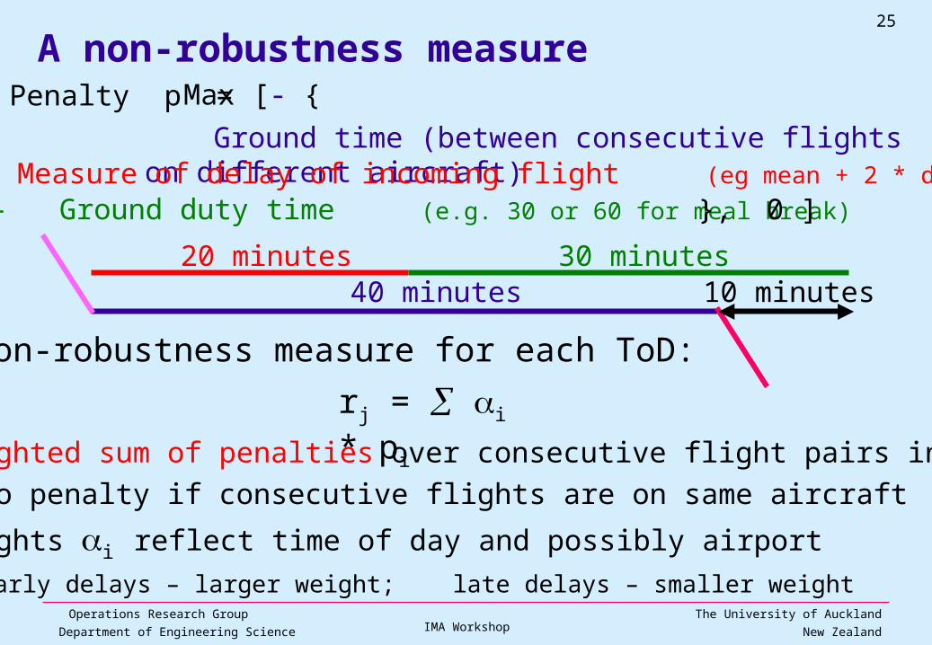
A non-robustness measure
Non-robustness measure for each ToD:
rj = i * pi
weighted sum of penalties over consecutive flight pairs in a ToD zero penalty if consecutive flights are on same aircraft
weights i reflect time of day and possibly airportearly delays – larger weight; late delays – smaller weight
Ground time (between consecutive flights on different aircraft)
40 minutes
- Measure of delay of incoming flight (eg mean + 2 * deviations)
20 minutes
- Ground duty time (e.g. 30 or 60 for meal break)
30 minutes
Penalty p = Max [- {
}, 0 ]
10 minutes
Operations Research GroupDepartment of Engineering Science
26
The University of AucklandNew ZealandIMA Workshop
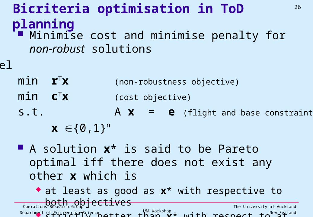
Bicriteria optimisation in ToD planning Minimise cost and minimise penalty for non-robust
solutions The model
min rTx (non-robustness objective)
min cTx (cost objective)
s.t. A x = e (flight and base constraints)
x {0,1}n
A solution x* is said to be Pareto optimal iff there does not exist any other x which is
at least as good as x* with respective to both objectives strictly better than x* with respect to at least one objective
Operations Research GroupDepartment of Engineering Science
27
The University of AucklandNew ZealandIMA Workshop
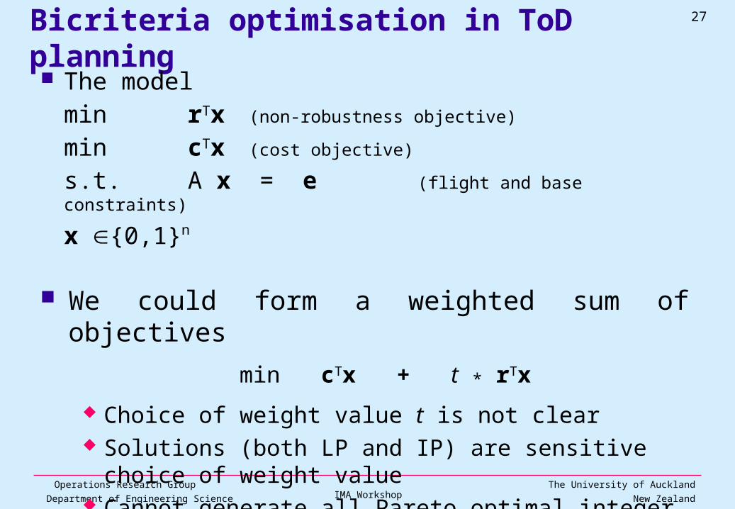
Bicriteria optimisation in ToD planning The model
min rTx (non-robustness objective)
min cTx (cost objective)
s.t. A x = e (flight and base constraints)
x {0,1}n
We could form a weighted sum of objectives
min cTx + t * rTx
Choice of weight value t is not clear Solutions (both LP and IP) are sensitive choice of weight value Cannot generate all Pareto optimal integer solutions
Operations Research GroupDepartment of Engineering Science
28
The University of AucklandNew ZealandIMA Workshop
300
350
400
450
500
550
600
650
400 410 420 430 440 450
Cost
No
n-r
ob
ust
nes
s .
LP Relaxation
IP Solution
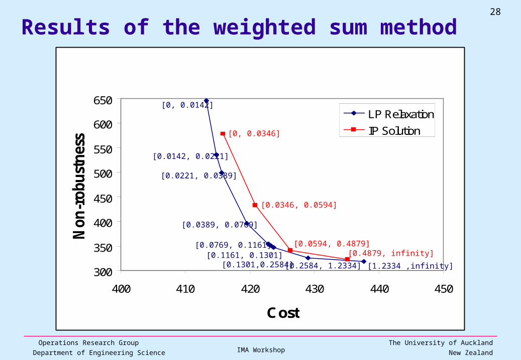
[0.0346, 0.0594]
[0, 0.0346]
[0.0594, 0.4879][0.4879, infinity]
[0, 0.0142]
[0.0142, 0.0221]
[0.0221, 0.0389]
[0.0389, 0.0769]
[0.0769, 0.1161][0.1161, 0.1301]
[0.1301,0.2584] [0.2584, 1.2334] [1.2334 ,infinity]
Results of the weighted sum method
Operations Research GroupDepartment of Engineering Science
29
The University of AucklandNew ZealandIMA Workshop
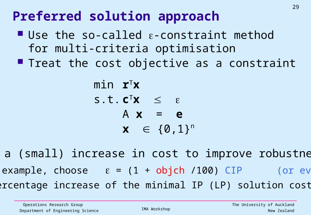
Preferred solution approach Use the so-called -constraint method for multi-criteria
optimisation Treat the cost objective as a constraint
Allow a (small) increase in cost to improve robustness for example, choose = (1 + objch /100) CIP (or even CLP) a percentage increase of the minimal IP (LP) solution cost
min rTxs.t. cTx
A x = ex {0,1}n
Operations Research GroupDepartment of Engineering Science
30
The University of AucklandNew ZealandIMA Workshop
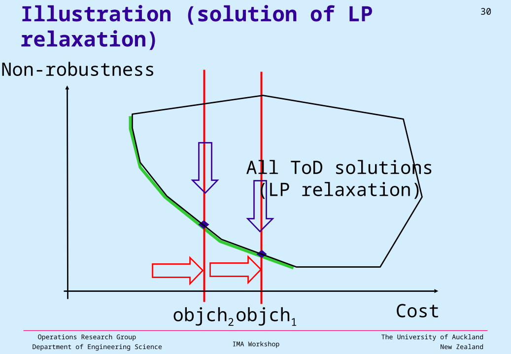
Illustration (solution of LP relaxation)
Cost
Non-robustness
All ToD solutions(LP relaxation)
objch1objch2
Operations Research GroupDepartment of Engineering Science
31
The University of AucklandNew ZealandIMA Workshop
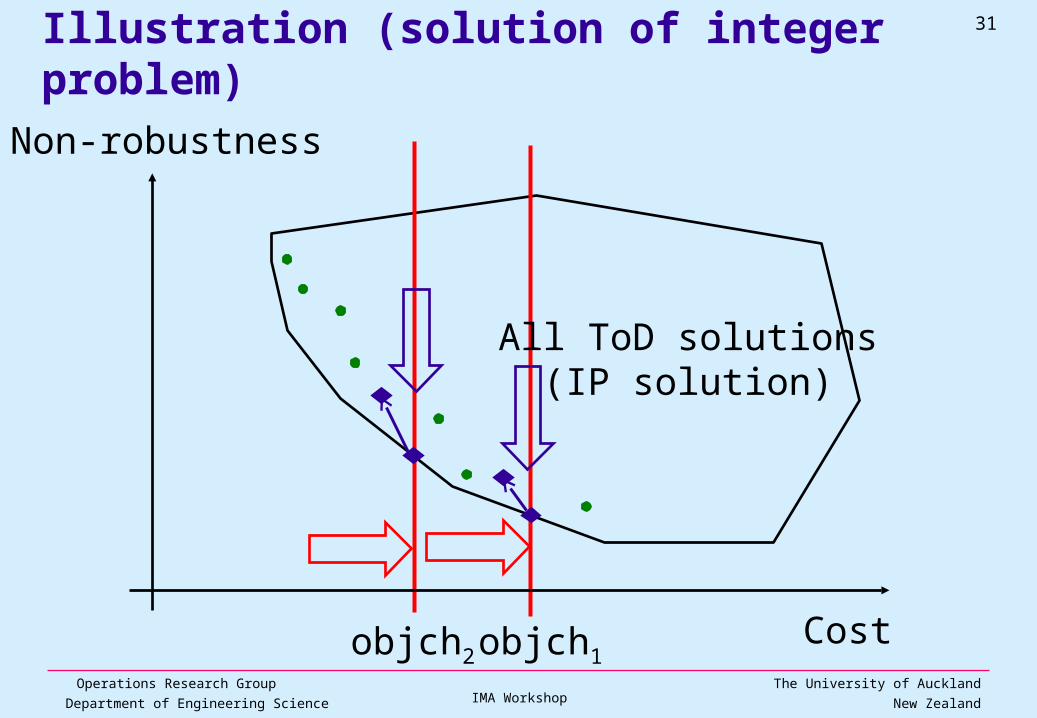
Illustration (solution of integer problem)
Cost
Non-robustness
All ToD solutions(IP solution)
objch1objch2
Operations Research GroupDepartment of Engineering Science
32
The University of AucklandNew ZealandIMA Workshop
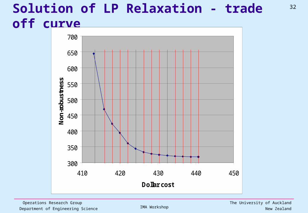
Solution of LP Relaxation - trade off curve
300
350
400
450
500
550
600
650
700
410 420 430 440 450
Dollar cost
Non
-rob
ustn
ess
Operations Research GroupDepartment of Engineering Science
33
The University of AucklandNew ZealandIMA Workshop
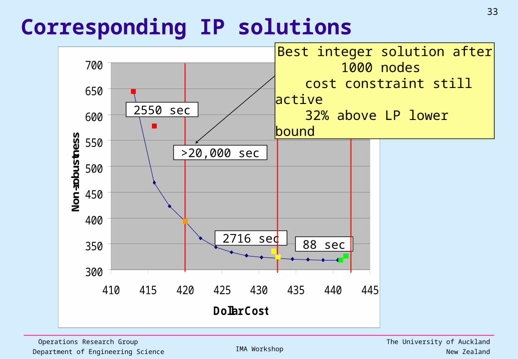
Corresponding IP solutions
300
350
400
450
500
550
600
650
700
410 415 420 425 430 435 440 445
Dollar Cost
Non
-rob
ustn
ess
2716 sec 88 sec
>20,000 sec
Best integer solution after 1000 nodes cost constraint still active32% above LP lower bound
2550 sec
Operations Research GroupDepartment of Engineering Science
34
The University of AucklandNew ZealandIMA Workshop
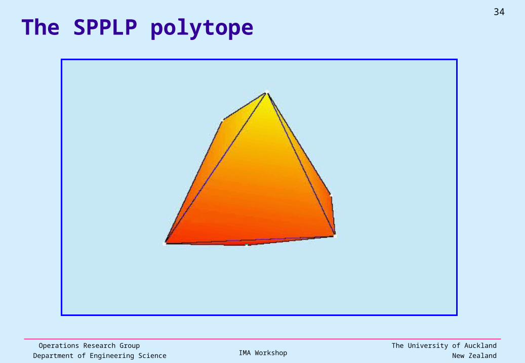
The SPPLP polytope
Operations Research GroupDepartment of Engineering Science
35
The University of AucklandNew ZealandIMA Workshop
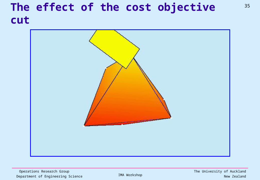
The effect of the cost objective cut
Operations Research GroupDepartment of Engineering Science
36
The University of AucklandNew ZealandIMA Workshop
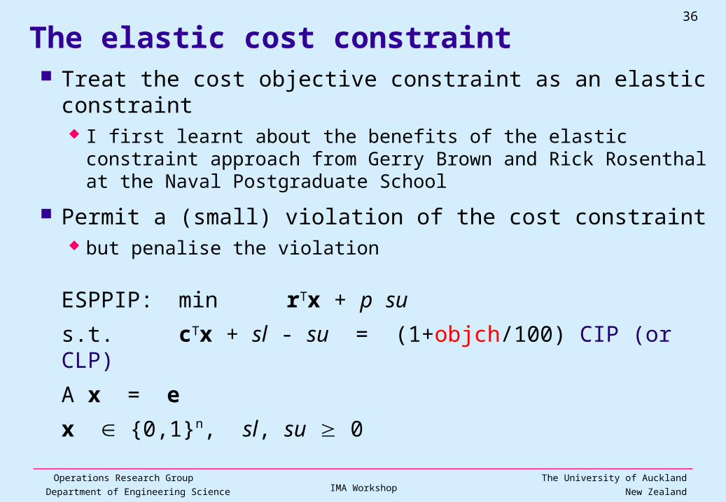
The elastic cost constraint Treat the cost objective constraint as an elastic constraint
I first learnt about the benefits of the elastic constraint approach from Gerry Brown and Rick Rosenthal at the Naval Postgraduate School
Permit a (small) violation of the cost constraint but penalise the violation
ESPPIP: min rTx + p su
s.t. cTx + sl - su = (1+objch/100) CIP (or CLP)
A x = e
x {0,1}n, sl, su 0
Operations Research GroupDepartment of Engineering Science
37
The University of AucklandNew ZealandIMA Workshop
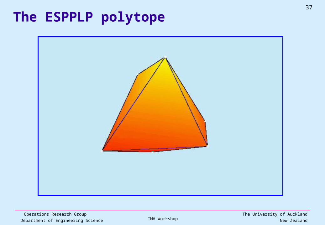
The ESPPLP polytope
Operations Research GroupDepartment of Engineering Science
38
The University of AucklandNew ZealandIMA Workshop
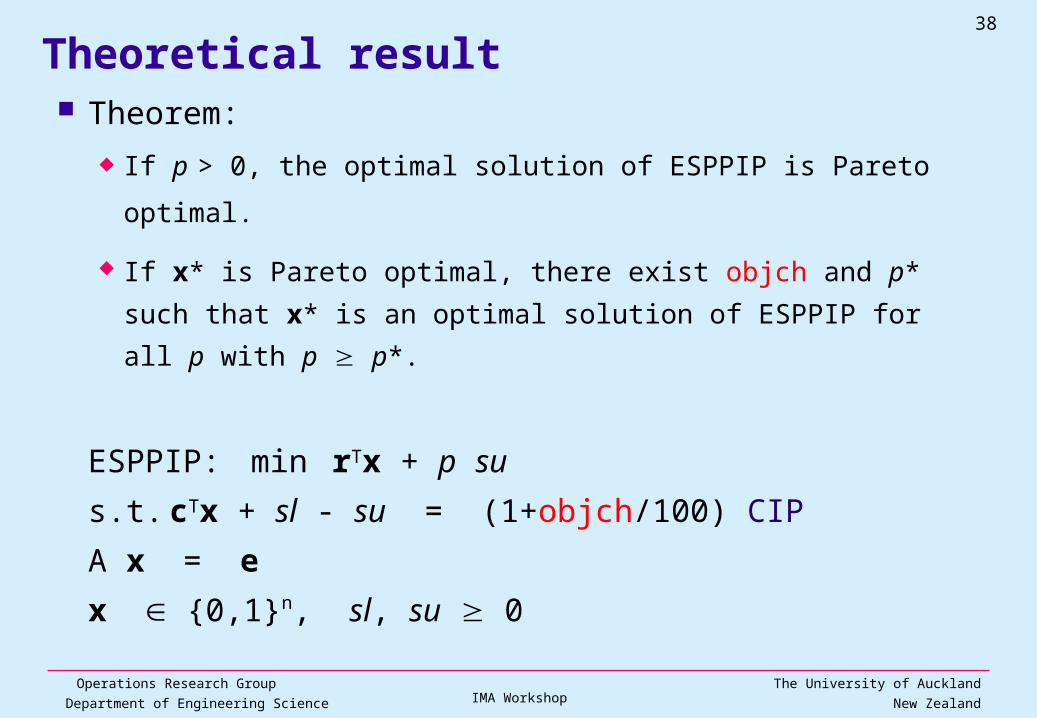
Theoretical result Theorem:
If p > 0, the optimal solution of ESPPIP is Pareto optimal.
If x* is Pareto optimal, there exist objch and p* such that x* is
an optimal solution of ESPPIP for all p with p p*.
ESPPIP: min rTx + p su
s.t. cTx + sl - su = (1+objch/100) CIP
A x = e
x {0,1}n, sl, su 0
Operations Research GroupDepartment of Engineering Science
39
The University of AucklandNew ZealandIMA Workshop
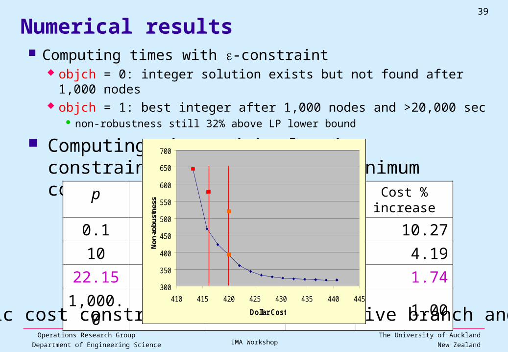
Computing times with elastic constraint (objch=1%) when minimum cost is 416.0
Numerical results Computing times with -constraint
objch = 0: integer solution exists but not found after 1,000 nodes objch = 1: best integer after 1,000 nodes and >20,000 sec
non-robustness still 32% above LP lower bound
p B&B nodes IP time Violation Cost % increase
0.1 62 2534.9 38.56 10.27
10 98 4338.6 13.28 4.19
22.15 52 1330.7 3.11 1.74
1,000.0 859 29525.8 0.00 1.00
Elastic cost constraint restores effective branch and bound
300
350
400
450
500
550
600
650
700
410 415 420 425 430 435 440 445
Dollar Cost
Non
-rob
ustn
ess
Operations Research GroupDepartment of Engineering Science
42
The University of AucklandNew ZealandIMA Workshop
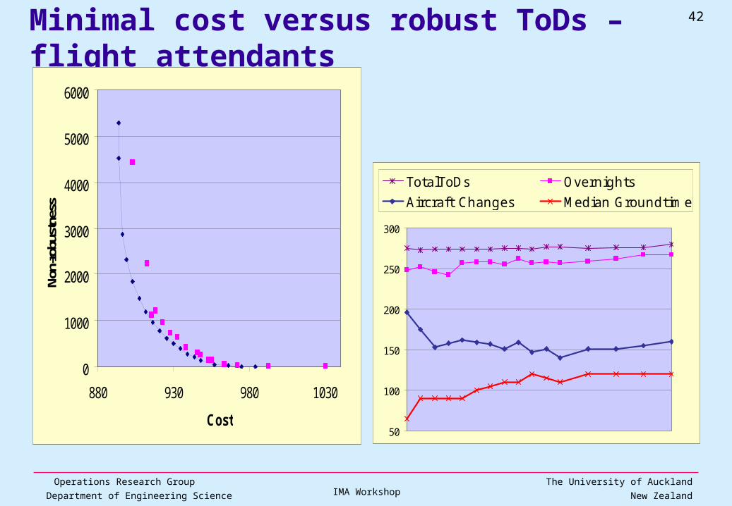
Minimal cost versus robust ToDs – flight attendants
0
1000
2000
3000
4000
5000
6000
880 930 980 1030
Cost
Non-
robu
stne
ss
50
100
150
200
250
300
TotalToDs Overnights
Aircraft Changes Median Groundtime
Operations Research GroupDepartment of Engineering Science
43
The University of AucklandNew ZealandIMA Workshop
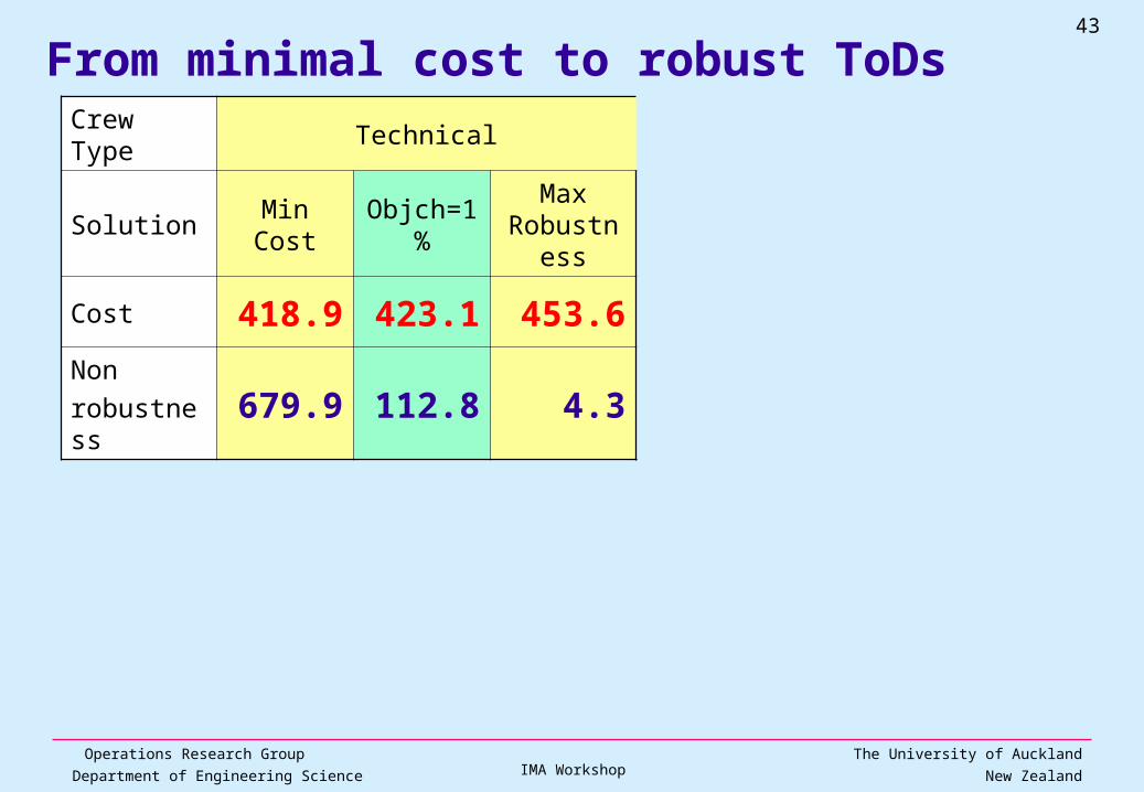
From minimal cost to robust ToDs
Crew Type Technical
Solution Min Cost Objch=1%Max
Robustness
Cost 418.9 423.1 453.6
Non
robustness679.9 112.8 4.3
Operations Research GroupDepartment of Engineering Science
44
The University of AucklandNew ZealandIMA Workshop
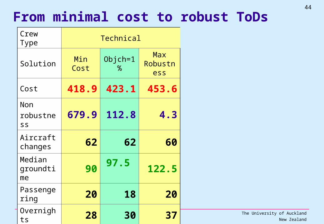
From minimal cost to robust ToDs
Crew Type Technical
Solution Min Cost Objch=1%Max
Robustness
Cost 418.9 423.1 453.6
Non
robustness679.9 112.8 4.3
Aircraft changes 62 62 60
Median groundtime 90 97.5 122.5
Passengering 20 18 20
Overnights 28 30 37
Operations Research GroupDepartment of Engineering Science
45
The University of AucklandNew ZealandIMA Workshop
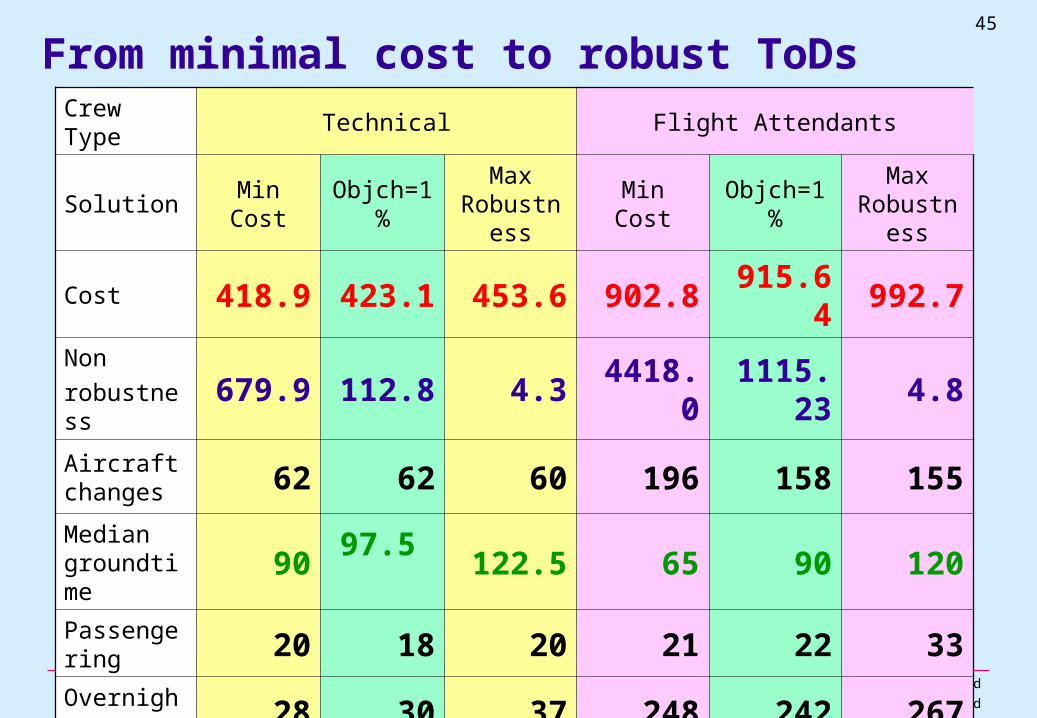
From minimal cost to robust ToDs
Crew Type Technical Flight Attendants
Solution Min Cost Objch=1%Max
RobustnessMin Cost Objch=1%
Max Robustness
Cost 418.9 423.1 453.6 902.8 915.64 992.7
Non
robustness679.9 112.8 4.3 4418.0 1115.23 4.8
Aircraft changes 62 62 60 196 158 155
Median groundtime 90 97.5 122.5 65 90 120
Passengering 20 18 20 21 22 33
Overnights 28 30 37 248 242 267
Operations Research GroupDepartment of Engineering Science
46
The University of AucklandNew ZealandIMA Workshop
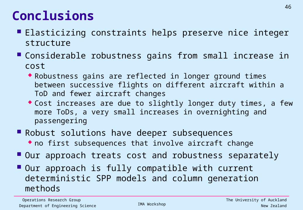
Conclusions Elasticizing constraints helps preserve nice integer structure Considerable robustness gains from small increase in cost
Robustness gains are reflected in longer ground times between successive flights on different aircraft within a ToD and fewer aircraft changes
Cost increases are due to slightly longer duty times, a few more ToDs, a very small increases in overnighting and passengering
Robust solutions have deeper subsequences no first subsequences that involve aircraft change
Our approach treats cost and robustness separately Our approach is fully compatible with current deterministic
SPP models and column generation methods
Operations Research GroupDepartment of Engineering Science
47
The University of AucklandNew ZealandIMA Workshop
Future work System should be easy to use:
Permitted cost increase (objch) is specified by management Dynamically modify the elastic penalty during the optimisation
to control cost violation keep elastic penalty cost as small as possible
Need to determine weights in rj = i * pi
Equal unit weights used so far
Compare results of all three approaches Use the SimAir package currently being developed by Georgia
Tech and the National University of Singapore