ISSN 1055-1425

August 2009

This work was performed as part of the California PATH Program of the University of California, in cooperation with the State of California Business, Transportation, and Housing Agency, Department of Transportation, and the United States Department of Transportation, Federal Highway Administration.

The contents of this report reflect the views of the authors who are responsible for the facts and the accuracy of the data presented herein. The contents do not necessarily reflect the official views or policies of the State of California. This report does not constitute a standard, specification, or regulation.

Final Report for Task Order 6203

CALIFORNIA PATH PROGRAMINSTITUTE OF TRANSPORTATION STUDIESUNIVERSITY OF CALIFORNIA, BERKELEY

Bicycle Detection and Operational Concept at Signalized Intersections

UCB-ITS-PRR-2009-37California PATH Research Report

Steven E. Shladover, ZuWhan Kim, Meng Cao, Ashkan Sharafsaleh, Jingquan Li, Kai Leung

CALIFORNIA PARTNERS FOR ADVANCED TRANSIT AND HIGHWAYS

Bicycle Detection and Operational Concept at Signalized Intersections

PATH Research Report on Task Order 6203

Steven E. Shladover, ZuWhan Kim, Meng Cao, Ashkan Sharafsaleh, Jingquan Li and Kai Leung

i

ii

Abstract In support of efforts to improve traffic signal timing to accommodate the needs of bicyclists, video observations have been made of the timing of bicyclists’ intersection crossing maneuvers. The processed data have yielded cumulative distributions of the crossing speeds of bicyclists who did not have to stop at the intersection and the start-up times and final crossing speeds of the bicyclists who had to cross from a standing start. A unique feature of these data is the timing information relative to the traffic signal, which will be essential for determining signal phase durations. Based on the detailed quantitative characterizations of bicyclist speeds and start-up times at signalized intersections, sample signal timing criteria have been defined to accommodate the 50%ile, 80%ile and 90%ile of bicyclists. The results indicate the soundness of the basic approach, but with a recommendation to account for all the relevant explanatory variables, including the bicycling population, roadway grade, mainline traffic speed and volume and the visibility of the mainline traffic by the bicyclists waiting to cross, in addition to the intersection width, in order to produce fully consistent results. A traffic microsimulation of a high-volume suburban arterial corridor has been used to show that moderate increases in the minimum green time for cross streets should have a negligible impact on delays and queuing along the mainline arterial. Experiments were conducted to determine the ability of commercially available traffic detection systems to detect a minimum-size bicycle with a minimum-size rider. These tests included Type D inductive loops of two sizes (3 feet square and 6 feet square), Sensys Networks magnetometers, and a Traficon video image processing system. Key Words: Bicycling, traffic detection, traffic signal timing

iii

iv

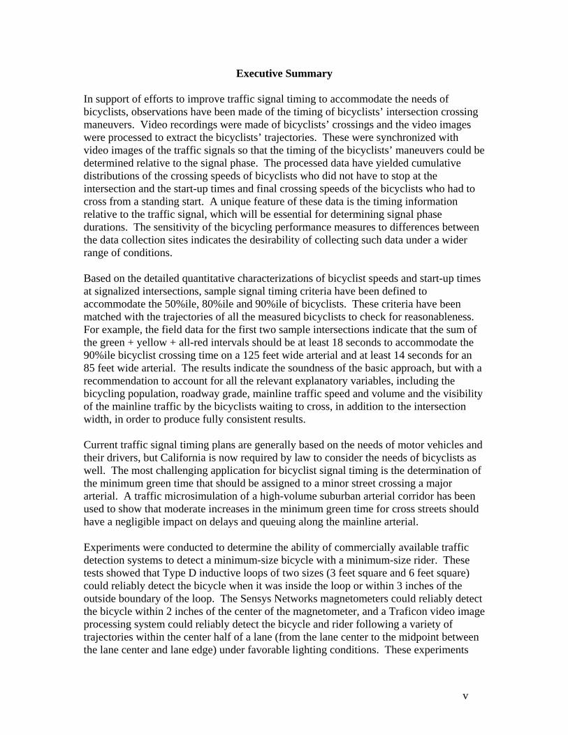
Executive Summary In support of efforts to improve traffic signal timing to accommodate the needs of bicyclists, observations have been made of the timing of bicyclists’ intersection crossing maneuvers. Video recordings were made of bicyclists’ crossings and the video images were processed to extract the bicyclists’ trajectories. These were synchronized with video images of the traffic signals so that the timing of the bicyclists’ maneuvers could be determined relative to the signal phase. The processed data have yielded cumulative distributions of the crossing speeds of bicyclists who did not have to stop at the intersection and the start-up times and final crossing speeds of the bicyclists who had to cross from a standing start. A unique feature of these data is the timing information relative to the traffic signal, which will be essential for determining signal phase durations. The sensitivity of the bicycling performance measures to differences between the data collection sites indicates the desirability of collecting such data under a wider range of conditions. Based on the detailed quantitative characterizations of bicyclist speeds and start-up times at signalized intersections, sample signal timing criteria have been defined to accommodate the 50%ile, 80%ile and 90%ile of bicyclists. These criteria have been matched with the trajectories of all the measured bicyclists to check for reasonableness. For example, the field data for the first two sample intersections indicate that the sum of the green + yellow + all-red intervals should be at least 18 seconds to accommodate the 90%ile bicyclist crossing time on a 125 feet wide arterial and at least 14 seconds for an 85 feet wide arterial. The results indicate the soundness of the basic approach, but with a recommendation to account for all the relevant explanatory variables, including the bicycling population, roadway grade, mainline traffic speed and volume and the visibility of the mainline traffic by the bicyclists waiting to cross, in addition to the intersection width, in order to produce fully consistent results. Current traffic signal timing plans are generally based on the needs of motor vehicles and their drivers, but California is now required by law to consider the needs of bicyclists as well. The most challenging application for bicyclist signal timing is the determination of the minimum green time that should be assigned to a minor street crossing a major arterial. A traffic microsimulation of a high-volume suburban arterial corridor has been used to show that moderate increases in the minimum green time for cross streets should have a negligible impact on delays and queuing along the mainline arterial. Experiments were conducted to determine the ability of commercially available traffic detection systems to detect a minimum-size bicycle with a minimum-size rider. These tests showed that Type D inductive loops of two sizes (3 feet square and 6 feet square) could reliably detect the bicycle when it was inside the loop or within 3 inches of the outside boundary of the loop. The Sensys Networks magnetometers could reliably detect the bicycle within 2 inches of the center of the magnetometer, and a Traficon video image processing system could reliably detect the bicycle and rider following a variety of trajectories within the center half of a lane (from the lane center to the midpoint between the lane center and lane edge) under favorable lighting conditions. These experiments

v

vi

did not address adverse weather or visibility conditions, so they do not indicate viability of the video system under all possible conditions. The magnetic detector results show the ability of the Type D loops to provide good coverage of a lane (6 foot loop for full width traffic lane or 3 foot loop for narrow bicycle lane), while the Sensys Networks magnetometers would have to be placed within 4 inches of each other throughout the area in which bicycles must be detected. The results from this project should be useful to traffic engineers in several ways: - providing initial guidance regarding the minimum amount of time that should be

allocated for bicyclists who need to cross major arterials at signalized intersections; - providing reassurance that increasing minimum green intervals for minor arterials

crossing major arterials should not have a significant adverse effect on mainline traffic;

- showing that Type D loop detectors should be able to detect a child bicyclist riding a small bicycle with minimum metallic content (if the detectors are properly calibrated).

vii

viii

Table of Contents

Abstract ______________________________________________________________ iii

Executive Summary ____________________________________________________ v

1 Introduction _______________________________________________________ 1

2 Literature Review __________________________________________________ 3

3 Field Data Collection on Bicyclist Crossing Behavior _____________________ 7

4 Analysis of Bicyclist Crossing Field Data ______________________________ 15

5 Simulation of Impacts on Traffic _____________________________________ 24

6 Conclusions and Recommendations on Signal Timing ___________________ 27

7 Testing of Bicyclist Detection Capabilities of Existing Traffic Detection Systems

__________________________________________________________________33

8 Conclusions ______________________________________________________ 37

9 References _______________________________________________________ 39

ix

x

List of Figures

Figure 1 Video Data Collection Sites at Telegraph Ave. and Russell St. in Berkeley (left) and at El Camino Real and Park Blvd. in Palo Alto (right) ......................................................................... 8

Figure 2 Data Collection Installation at Park Blvd. and El Camino in Palo Alto ........................................... 9 Figure 3 Data Collection Installation at Russell St. and Telegraph in Berkeley ........................................... 10 Figure 4 An example image (left); corner feature tracks (middle); and background subtraction blobs

(right) .......................................................................................................................................... 11 Figure 5 Two-level grouping can be used for varying sizes of objects: cluster-level (left) and object level

(right) .......................................................................................................................................... 12 Figure 6 Discrimination of bicycles from passenger vehicles by applying an SVM classifier on texture

information. ................................................................................................................................ 12 Figure 7 Video Playback Tool Showing Image Processing Software Tracking Bicyclists Across

Intersection (El Camino Real at Park) ........................................................................................ 13 Figure 8 Example of Extraction of Needed Values for Standing Start from Bicyclist Trajectory Plot ....... 14 Figure 9 Cumulative Distributions and Histograms of Speed of Rolling Start Bicycles (mph) .................. 16 Figure 10 Cumulative Distributions and Histograms of Offset Times for Standing Start Bicyclist Crossings

.................................................................................................................................................... 17 Figure 11 Cumulative Distributions and Histograms of Final Crossing Speed for Standing Start Bicyclist

Crossings (mph) .......................................................................................................................... 18 Figure 12 – Cross-Plot of Standing Start Offset Times and Final Speeds at Park Blvd. .............................. 18 Figure 13 Distributions of Total Time for Bicyclists to Cross El Camino Real from a Standing Start ....... 20 Figure 14 Cumulative Distributions of Offset Times for Standing Start Bicyclist Crossings, Showing Effect

of Queuing at Park Blvd. ............................................................................................................ 20 Figure 15 Distribution of Duration of Green Phase (s) When Bicyclists Were Crossing El Camino Real at

Park Blvd. ................................................................................................................................... 21 Figure 16 Distribution of Duration of Green Phase (s) When Bicyclists Were Crossing Telegraph at

Russell St. ................................................................................................................................... 22 Figure 17 Completion Times of Bicyclist Crossings from Standing Start, Relative to Yellow Onset, at El

Camino Real and Park Blvd. ...................................................................................................... 23 Figure 18 VISSIM Simulation Network of El Camino Real Corridor in Palo Alto and Mountain View, CA

.................................................................................................................................................... 25 Figure 19 Application of Signaling Criteria Based on 50, 80 and 90%ile Bicyclist Crossings to All

Crossings from a Standing Start at Park Blvd. in Palo Alto ....................................................... 30 Figure 20 Application of Signaling Criteria Based on 50, 80 and 90%ile Non—Queued Bicyclist

Capabilities to All Crossings from a Standing Start at Park Blvd. in Palo Alto ......................... 30 Figure 21 Application of Signaling Criteria Based on 50, 80 and 90%ile Bicyclist Capabilities to All

Eastbound Crossings from a Standing Start at Russell Street in Berkeley ................................. 31 Figure 22 Application of Signaling Criteria Based on 50, 80 and 90%ile Bicyclist Capabilities to All

Westbound Crossings from a Standing Start at Russell Street in Berkeley ................................ 31 Figure 23 Dependence of Signal Duration Criteria Based on 50, 80 and 90%ile Bicyclist Capabilities on

Street Crossing Width ................................................................................................................. 32 Figure 24 Test Bicycle Aligned with Edge of 3-Foot Type D Loop (left) and 6-Foot Type D Loop (right) 33 Figure 25 Test Bicycle Approaching Sensys Networks Sensor (left), with Wireless Link to Sensys Access

Point on Pole (right) ................................................................................................................... 34 Figure 26 Nominal-Size Bicyclist (4 feet tall, 90 pounds) Riding the Test Bicycle Just Inside the Lane

Boundary for Testing Video Detection System, Using Traficon Camera Mounted on Mast Arm (right in right photo) ................................................................................................................... 35

Figure 27 Schematic View of Traficon Video Detection Zones .................................................................. 35 List of Tables Table 1 Comparison of Intersections Where Data Were Collected………………………………………. 10

Table 2 Video Detection Test Conditions…………………………………………………………………….36

xi

xii

1 Introduction This project was originated with the intention of evaluating alternative technologies for detecting bicyclists waiting at intersections, to identify the most promising available alternatives and enhancing them if necessary. A literature review of the existing technologies was prepared and some candidates were prepared for testing. A new video image processing approach was also developed and tested on video images of bicyclists at a public intersection in Berkeley and at a test intersection at the University of California’s Richmond Field Station. However, the direction of the project changed with the passage of California Assembly Bill 1581 (AB 1581). In October 2007 AB1581 amended the California Vehicle Code, stating that “Bicyclists and motorcyclists are legitimate users of roadways in California” and requiring traffic-actuated signals to “be installed and maintained so as to detect lawful bicycle or motorcycle traffic on the roadway.” AB 1581 also calls on the California Department of Transportation (Caltrans) to establish “uniform standards, specifications and guidelines for the detection of bicycles and motorcycles by traffic-actuated signals and related signal timing” (italics added). This stimulated the need for Caltrans to determine how to specify the minimum green signal intervals throughout the state to give bicyclists sufficient time to cross wide arterials from a standing start. Of course, any increase in the green time allocated to minor cross streets has to be taken away from the time available for mainline traffic on the arterial, so a trade-off must be made between the needs of the mainline drivers and the needs of the crossing bicyclists. The current default duration of the minimum green interval is 4 seconds in California, but there are precedents for increasing this to longer times at wide intersections with heavy bicyclist traffic, especially where those bicyclists include school children. If bicyclists could be detected reliably at intersection approaches and clearly distinguished from motor vehicles it would be possible to modify the signal timing so that the bicyclists would receive longer green times than the motor vehicles. In this way, the longer green intervals would only be triggered when bicyclists are present, minimizing the negative effects on mainline green time. Unfortunately, although bicycle classification is possible with state of the art image processing technology, it is not yet sufficiently reliable or mature for practical deployment in the field, so bicyclists and motor vehicles will be receiving the same green signal time for the foreseeable future. This increases the urgency of determining the minimum length of green that is really needed by the bicyclists, since this green interval will have to apply all the time, with or without bicyclists being present. The alternative available for bicyclists to actuate a green signal to cross a busy arterial is pushing the pedestrian call button (where one is available). This provides a significantly longer green crossing time than the minimum that bicyclists should need, since it has to be set based on pedestrian walking speed, thereby incurring a significant efficiency penalty on the mainline traffic.

1

1.1 New Information Needed In order to make intelligent decisions about the length of green intervals to accommodate bicyclists, several kinds of information are needed:

- time needed for bicyclists to start up from a stop after their signal turns green - speed of bicyclists crossing a wide arterial, once they have reached their cruising

speed - dependence of bicyclist crossing times on street width - dependence of crossing time on road geometry details (grade, arterial crown) - dependence of crossing time performance on bicyclist demographics (especially

age) - effects of shortened green time on mainline traffic conditions, with both

coordinated and independent signals. Unfortunately, very little such information is available in the literature, which means that it was necessary to create much of that information for this project. 1.2 Relevant Prior Literature It is not easy to collect quantitative microscopic data about bicycling, and only limited resources have been available to support efforts to collect such data. This has tended to limit the breadth and depth of the information available in the literature. The most directly relevant prior work is the 1995 review paper by Wachtel et. al., which summarized a variety of preceding studies to point toward signal timing recommendations [1]. The data cited directly in the paper are relatively limited and are described only in terms of mean crossing times and speeds. In the absence of more detailed data it is difficult to know how to apply the findings more widely. The second relevant work is the 2005 TRB paper by Rubins and Handy [2], which summarizes an extensive set of bicyclist crossing observations in Davis, CA. These data, which represent total crossing times at intersections of varying widths, show significant scatter, making it challenging to use them as the basis for specific signal timing recommendations. Regressions showed the mean value of crossing time as a function of crossing width, and the authors derived estimates of fixed start-up time and crossing speed from these ensemble statistics. They focused on 2%ile and 15%ile statistics for formulating their recommendations, but the full distributions of crossing times were not reported, which makes it impossible to apply other percentile criteria based on their data. 1.3 Need for New Data Collection The decision about increasing minimum green intervals to accommodate bicyclists could potentially have significant impacts on arterial traffic throughout California. Therefore,

2

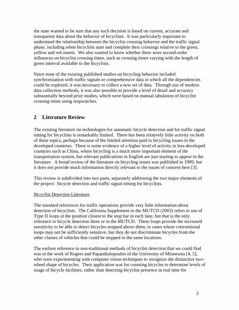
the state wanted to be sure that any such decision is based on current, accurate and transparent data about the behavior of bicyclists. It was particularly important to understand the relationship between the bicyclist crossing behavior and the traffic signal phase, including when bicyclists start and complete their crossings relative to the green, yellow and red onsets. We also wanted to know whether there were second-order influences on bicyclist crossing times, such as crossing times varying with the length of green interval available to the bicyclists. Since none of the existing published studies on bicycling behavior included synchronization with traffic signals or comprehensive data in which all the dependencies could be explored, it was necessary to collect a new set of data. Through use of modern data collection methods, it was also possible to provide a level of detail and accuracy substantially beyond prior studies, which were based on manual tabulation of bicyclist crossing times using stopwatches.

2 Literature Review The existing literature on technologies for automatic bicycle detection and for traffic signal timing for bicyclists is remarkably limited. There has been relatively little activity on both of these topics, perhaps because of the limited attention paid to bicycling issues in the developed countries. There is some evidence of a higher level of activity in less-developed countries such as China, where bicycling is a much more important element of the transportation system, but relevant publications in English are just starting to appear in the literature. A broad review of the literature on bicycling issues was published in 1999, but it does not provide much information directly relevant to the issues of concern here [3]. This review is subdivided into two parts, separately addressing the two major elements of the project: bicycle detection and traffic signal timing for bicyclists. Bicyclist Detection Literature The standard references for traffic operations provide very little information about detection of bicyclists. The California Supplement to the MUTCD (2003) refers to use of Type D loops at the position closest to the stop bar in each lane, but that is the only reference to bicycle detection there or in the MUTCD. These loops provide the increased sensitivity to be able to detect bicycles stopped above them, in cases where conventional loops may not be sufficiently sensitive, but they do not discriminate bicycles from the other classes of vehicles that could be stopped in the same locations. The earliest reference to non-traditional methods of bicyclist detection that we could find was in the work of Rogers and Papanikolopoulos of the University of Minnesota [4, 5], who were experimenting with computer vision techniques to recognize the distinctive two-wheel shape of bicycles. Their application was for counting bicycles to determine levels of usage of bicycle facilities, rather than detecting bicyclist presence in real time for

3

triggering a bicycle signal. Their laboratory prototype worked at up to 8 video frames per second with up to two bicycles per image, and an accuracy level of about 70%. The next study of bicyclist detection was led in 2001 by Prof. David Noyce, then at the University of Massachusetts (now at the University of Wisconsin) [6-8]. The Noyce work began with a broad review of the candidate detection technologies [6], including traditional inductive loops and pneumatic tube detectors, but also considering microwave, ultrasonic, acoustic, piezoelectric, magnetic, passive and active infrared and video image processing. The preferred technologies chosen for further study were video image processing and active infrared, because their imaging capabilities held the potential to discriminate bicycles from other vehicle classes. Experiments were conducted with the AutoSense II Active Infrared Imaging Sensor (no longer available, but superseded by the OSI AutoSense 600 Series) because it already had a motorcycle classification capability, which could be the starting point for bicyclist classification. The results showed that 97% of the bicyclists were detected, but only 77% were classified correctly (as motorcycles). With further enhancements to the classification algorithms, the authors were subsequently able to increase the percentage of correct classifications to 92% (with the remaining problems involving cases with four or more objects moving beneath the sensor simultaneously) [8]. A review of bicycle and pedestrian detection technologies was conducted for the Minnesota DOT by SRF Consulting in 2003 [9]. This work focused on testing the chosen detectors on a bicycle trail, rather than a public road shared with vehicle traffic, for one day in daylight. The detectors included an Autoscope Solo video image processing system, MS Sedco SmartWalk 1400 radar, ASIM DT 272 passive infrared and ultrasonic detector and a Diamond TTC infrared traffic counter. The distinctions between which of these were designed for real-time use and which were for collecting offline historical usage data was not made clear in the report. The first two detectors were mounted overhead, while the last two were pointed horizontally, mounted at heights of 4 ft. and 3 ft. respectively. The results of the limited testing indicated 100% detection of bicyclists by the Autoscope and ASIM, and 96% detection by the other two, but there was no attempt at classifying bicyclists relative to other vehicle categories since this was beyond the capabilities of these detectors. A parallel evaluation of a wide range of traffic detectors was done by the University of Utah at about the same time [10]. This review made only brief mention of bicycle detectors, grouped with pedestrian detectors, and included a table listing the detectors that were tested by SRF in [9] and the results of those tests. Kimley-Horn Associates performed a field test evaluation of bicyclist detection for Caltrans District 4 in 2004, producing a detailed report on the results [11]. Their work focused on applications where the bicyclists had to be detected in left turn pockets and in the traffic lanes of minor side streets, where they were waiting to cross a major arterial (El Camino Real on the San Francisco Peninsula), representing a more challenging environment than most of the previous projects. They used both Type-D inductive loops and video image processing systems to detect bicyclists, but did not try to discriminate them from other vehicles. Four video image processing systems (from Peek, Traficon,

4

Econolite and Iteris) were tested, all using the same Cohu monochrome camera, and the vendors of all four systems were invited to adjust their systems on-site for best performance. The Iteris video system was found to be most effective in these tests, but the conditions were generally benign (clear weather) and the vendors were all encouraged to tune up their systems for optimal effectiveness, which would typically not be the case for a routine field deployment. The detections were very close to 100% for test periods when the automatic detections were compared with manual examination of video recordings. There were a few false detections caused by pedestrians and a few missed detections of bicyclists in the detection zone. Much useful knowledge was documented about the practical details involved in the implementation and operation of the system under a wide range of real-world conditions. The Toole Design Group and the University of North Carolina did a comprehensive national review of pedestrian and bicycle transportation data in 2005, which includes some information about approaches to bicyclist detection for purposes of counting the volume of bicycle traffic [12]. Most of these automatic detection and counting systems provided only the user counts, and could not distinguish pedestrians from bicyclists. Only the active infrared and video technologies could distinguish user types (bicyclists from pedestrians), but this required off-line interpretation of data by people. Consequently, these would not be usable for real-time applications such as issuing calls for signal phase changes. Traffic Signal Timing for Bicyclists The literature on traffic signal timing for bicyclists is even more limited than that on bicyclist detection. The most widely cited reference on this topic is a 1995 ITE paper by Wachtel, Forester and Pelz [1], which synthesizes findings from a variety of prior research, including the extensive work by Taylor [11]. The key challenges in this work involve obtaining accurate and representative measurements of the intersection-crossing behavior of bicyclists (perception/reaction times, speeds and accelerations) and determining how to accommodate the wide diversity in that behavior. This is a particular concern where the bicycling population includes many elementary school children or senior citizens, who will need considerably more time to cross an intersection than high school or college students. This points to the likely need for population-specific calibrations of signal timing, not just calibrations based on physical dimensions of the intersection. Bicyclists who enter the intersection moving at full speed during the green or yellow phases must be considered when determining the length of the yellow and red clearance intervals. Bicyclists who are already stopped at the intersection and start up on a new green phase must be considered in determining the length of the minimum green interval. Taylor measured mean speeds of about 23 km/h (14 mph) in Austin, TX, while Wachtel reported mean speeds at six intersections in Palo Alto, CA ranging from 9 mph to 16.5 mph, with the variations depending on the relative percentages of elementary, high school and college students among the bicyclists crossing at each intersection. After associating the faster bicyclists with higher braking capabilities (0.25 g) and the slower bicyclists with

5

lesser braking capabilities (0.125 g), Wachtel concluded that the yellow intervals defined for motorists would also be adequate for bicyclists, so no special adjustments would be recommended. The all-red interval was more troublesome, because Wachtel estimated that it would be necessary to calculate this based on the 98%ile crossing times of bicyclists in order to satisfy safety concerns. He used speeds of 6 mph for children, 8 mph for casual adult cyclists and 12 mph for fast cyclists, leading to a clearance time of 11.6 s for the middle speed bicyclists crossing a 130 ft wide arterial (more than three times longer than the clearance time for a car traveling at 25 to 30 mph). Since all-red clearance intervals longer than 2 s are generally discouraged, it would clearly not be practical to implement such a long all-red interval, which could have multiple adverse impacts on traffic flow and safety. Wachtel noted that the sum of the length of the green interval, plus the yellow and all-red intervals, needs to be sufficient to enable a stopped bicyclist to accelerate from a stop and clear the intersection before the crossing traffic receives its green signal. The key bicycling performance measures needed to determine this are thus the acceleration rate and maximum speed achieved by the bicycling population. Wachtel reported acceleration ranges from 0.046 to 0.11 g, depending on bicyclist level of effort [1], while Taylor reported a mean acceleration over a distance of 150 feet as 0.043 g and over 60 feet as 0.12 g [13]. They recognized that the signal interval lengths need to be governed by the slower bicyclists, not the faster ones. Wachtel recommended focusing attention on the difference between the intersection crossing time from a standing start and the crossing time when rolling at constant cruise speed, which is the sum of the perception-reaction time and v/2a, where v and a are the bicyclist cruise speed and acceleration respectively. For the Palo Alto intersections where he collected data, this sum was in the range of 4 to 6 seconds, so to be conservative he assumed a value of 6 seconds. If the yellow interval lasts a minimum of 3 seconds, this implies that even a green interval as short as 3 seconds could be sufficient (provided that the all-red interval is long enough for bicyclists to clear the intersection on an old green). Because of the previously-observed limitations on the all-red interval duration, it may be necessary to increase the minimum green interval accordingly to compensate for the impracticality of extending the all-red interval to the full duration that would be needed for a slow bicyclist to cross a wide arterial. A few more recent references have built on the earlier work of Wachtel and Taylor. The City of Toronto developed its own requirements for green time and clearance intervals for bicyclists, building on review of the prior literature [14]. They chose to assume bicyclist speeds of 4.7 m/s (10.5 mph) for determining the minimum green and all red durations, and 7.4 m/s (16.5 mph) for determining the yellow duration. For their amber duration calculations, they assumed deceleration of 0.24 g and perception/reaction time of 1.0 s, while for determining the minimum green duration they assumed acceleration of 0.05 g and perception/reaction time of 2.6 s (bicyclist assumed less attentive while stopped awaiting a green signal than while approaching the intersection at full speed). They also recommended that in general the all-red interval should be extended by no more than one second beyond the motor vehicle requirement in order to accommodate bicyclists.

6

The most recent measurements of bicyclist behavior were reported from Davis, CA [2]. Digital video cameras were used to record bicycle movements at ten intersections, with a total of over 2000 bicyclist crossings in eleven hours of data. These data showed a range of speeds from 2.9 ft/s to 33 ft/s, with a mean value of 13.5 ft/s (9.2 mph) and median of 12.5 ft/s (8.5 mph). The authors suggested focusing on the 2%ile and 15%ile speeds in order to produce conservative recommendations for signal timing. For standing starts (to calculate minimum green times), these speeds were 5.33 and 8.25 ft/s (3.63 and 5.63 mph) respectively, while for constant rolling crossings of intersections (to calculate clearance intervals) they were 6.4 and 10.63 ft/s (4.36 and 7.25 mph) respectively. Their data showed that the average standing start could be described by a 3.1 second delay and a speed of 17.8 ft/s (12.1 mph), while the average rolling approach was described by a 2.1 second delay and a speed of 23.8 ft/s (16.2 mph), but the scatter in the data points was quite large.

3 Field Data Collection on Bicyclist Crossing Behavior 3.1 Data Collection System The quantification of bicyclist crossing behavior relied on digital video recording and offline video image processing of the bicyclist movements. This approach evolved from original work earlier in this project on use of video image processing as a means of detecting bicyclists and discriminating them from motor vehicles. A video camera was mounted on top of a mast at a height of 6 – 7 m, atop a trailer which was parked near the subject intersection. The location of the trailer was chosen to provide a clear view of the bicyclist crossing path, with the camera height selected to be high enough that passing vehicles could not occlude the view of the bicyclists. A second video camera was mounted at a height of 2 - 3 m, with a view of the traffic signal head governing the bicyclist crossing movement. An embedded computer (PC/104) equipped with an MPEG hardware compression board was used to convert the analog video signals into pairs of MPEG video clips. The video clips were synchronized to have less than 33 ms (one scan) error. 3.2 Selection of Host Sites The initial criteria for selection of host sites for the data collection were:

- high volume of bicyclist traffic - diversity of bicyclist population across sites - moderate to wide intersection width - available location for mounting video camera in an adjoining building or on the

parked trailer. - access to traffic signal controller for recording real-time signal phase information.

7

Access to the traffic signal controller was originally the primary criterion for choosing sites because of the importance of synchronizing the signal phase with the bicyclist crossing observations. This led to an initial focus on El Camino Real (SR-82) in Palo Alto, CA, where PATH has access to the Caltrans signal controller data for use on several other projects. Unfortunately, the first attempt to synchronize the signal data with the video data failed because of unexplained drop-outs and latencies in the signal data stream, so this method had to be abandoned in favor of using the second video camera, with video image processing to detect the signal phase changes. Much effort was expended trying to arrange with building owners for permission to mount our video cameras on the roofs or balconies or in the windows of their buildings overlooking the target bicyclist crossings. These efforts were largely unsuccessful, leading to the backup alternative of the camera mounted on the mast atop the trailer, which was originally developed for a different project. This outdoor arrangement provided more flexibility in choosing specific camera locations and angles, but it incurred the burdens of providing power for the equipment on the trailer, obtaining permits from the host cities, and keeping research staff on site with the trailer and its accompanying van for the entire duration of the data collection to ensure security of the equipment. It was also important to ensure that the parked trailer would not be so visually intrusive that it might cause bicyclists to slow down to take a closer look.

Figure 1 Video Data Collection Sites at Telegraph Ave. and Russell St. in Berkeley (left) and at El Camino Real and Park Blvd. in Palo Alto (right)

The two intersections that were finally selected for the data collection reported here were El Camino Real and Park Blvd. in Palo Alto, CA, which was recommended by the City of

8

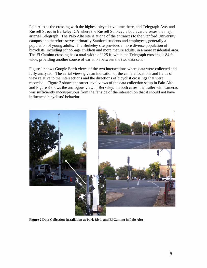
Palo Alto as the crossing with the highest bicyclist volume there, and Telegraph Ave. and Russell Street in Berkeley, CA where the Russell St. bicycle boulevard crosses the major arterial Telegraph. The Palo Alto site is at one of the entrances to the Stanford University campus and therefore serves primarily Stanford students and employees, generally a population of young adults. The Berkeley site provides a more diverse population of bicyclists, including school-age children and more mature adults, in a more residential area. The El Camino crossing has a total width of 125 ft, while the Telegraph crossing is 84 ft. wide, providing another source of variation between the two data sets. Figure 1 shows Google Earth views of the two intersections where data were collected and fully analyzed. The aerial views give an indication of the camera locations and fields of view relative to the intersections and the directions of bicyclist crossings that were recorded. Figure 2 shows the street-level views of the data collection setup in Palo Alto and Figure 3 shows the analogous view in Berkeley. In both cases, the trailer with cameras was sufficiently inconspicuous from the far side of the intersection that it should not have influenced bicyclists’ behavior.

Figure 2 Data Collection Installation at Park Blvd. and El Camino in Palo Alto

9

Figure 3 Data Collection Installation at Russell St. and Telegraph in Berkeley

There were many differences between the two intersections, contributing to differences in the observed statistics of bicyclist crossing behavior. These contrasts are summarized in Table 1.

Table 1 Comparison of Intersections Where Data Were Collected

10

3.3 Data Processing Algorithm After the video data are recorded in the field, they are analyzed in the laboratory to extract the information of interest. We have developed an image processing system that automatically detects moving objects in the video and generates their trajectories. Our tracking system combines the background subtraction algorithm and the feature tracking and grouping algorithm to robustly detect and track moving objects. In the background subtraction algorithm, a static background hypothesis is extracted from a sequence of images and a moving object is detected by pixel-by-pixel subtracting the current image frame from the background hypothesis. It shows good performance in good illumination conditions, and is therefore used by most previous work and commercial systems. However, it suffers problems with occlusions, presence of shadows, sudden illumination changes, and slow moving or stopped traffic. The feature tracking and grouping algorithm detects and tracks many small image patches (corner features) and groups them based on their position and motion. While it is more robust to occlusion, illumination, and shadow problems, it has difficulty in grouping objects moving at a similar speed. We developed a novel algorithm by combining the two algorithms to generate reliable object trajectories. It first generates corner trajectories and object blobs by applying standard feature tracking and background subtraction algorithms. Then, both the corner trajectories and object blobs are refined by cross-checking -- corner trajectories should be in a blob and a blob should contain at least one corner trajectory. This cross-checking procedure significantly increases the robustness and we can get reliable features, as shown in Figure 4.

Figure 4 An example image (left); corner feature tracks (middle); and background subtraction blobs (right)

The next step is to group these corner features into objects. The corner features are grouped into clusters and/or objects based on the proximity, motion history and background subtraction blob membership history. Probablistic reasoning was used and the parameters were determined by a semi-supervised learning algorithm. Two-level grouping can be used when object sizes vary as illustrated in Figure 5. In our data analysis, a single-level grouping with a fixed object (bicycle) size was used.

11

Figure 5 Two-level grouping can be used for varying sizes of objects: cluster-level (left) and object level (right)

It is also possible to discriminate the bicycles or pedestrians from motor vehicles. Since motor vehicles have distinct horizontal lines and uniform regions, we applied a Support Vector Machine (SVM) classifier on these texture information for the classification. A preliminary classification result is shown in Figure 6. We tested on a video clip with a challenging illumination condition (shadows of wind-blown trees). Among ten bicycles and four passenger cars in the video clip, only one bicycle was misclassified (shown in the middle frame of Figure 6).

More details of the algorithm are described in [15].

Figure 6 Discrimination of bicycles from passenger vehicles by applying an SVM classifier on texture information.

3. 4 Data Processing Procedure We applied a user interactive image processing tool based on the previously introduced tracking algorithm. The fully automated system can also deliver robust trajectories. However, our video clip covers a wide road and the image resolution was very poor on the far side. In addition, many bicyclists crossed the road using pedestrian crossings and it is very difficult to discriminate bicyclists from pedestrians. Therefore, it is more practical to use an interactive tool to ensure error-free detection. An operator manually confirmed, repositioned or manually marked the initial position of each bicyclist. The tracking was then done automatically but any visible tracking errors were fixed manually using the interactive tool. A screen shot of the interactive tool, with the image processing system's symbols identifying the bicyclists with a thick ellipse, is shown in Figure 7. More details

12

on the interactive system and the trajectory generation procedure are described in [15]. Note the superimposed image of the traffic signal from the second video camera, visible in the upper left corner of each image. An image processing tool was used to extract the signal phase from the image patch, and the result was shown to the user to ensure that the phase detection is correct.

Figure 7 Video Playback Tool Showing Image Processing Software Tracking Bicyclists Across Intersection (El Camino Real at Park)

The error of the start of the crossing time relative to the beginning of the green signal phase is less than 100 ms. The trajectories may contain some errors from the conversion from image to world coordinates (calibration errors) and/or tracking errors due to poor image resolution. Such an error can be up to 1 m within the intersection box and even larger behind the stop bar on the far side of the intersection, where the image resolution is poor. Therefore, determining the crossing starting time from the trajectory alone may result in errors, but this is not a major concern because we are primarily interested in the timing relative to the green signal onset. The output of the video image processing software, as applied using the playback tool, is a plot of the location of the bicyclist crossing the intersection versus time. The traffic signal phase information is used to establish the reference time. The start of the green phase is defined as time zero for each crossing trajectory, and the times of the yellow and red onsets are marked by vertical yellow and red lines on the plots. An example of the plot that is generated for each bicyclist crossing is shown in Figure 8.

13

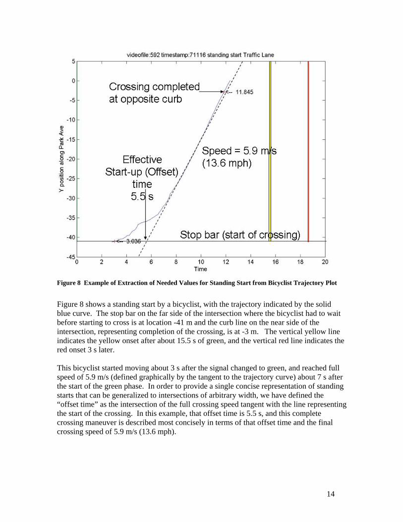
Figure 8 Example of Extraction of Needed Values for Standing Start from Bicyclist Trajectory Plot

Figure 8 shows a standing start by a bicyclist, with the trajectory indicated by the solid blue curve. The stop bar on the far side of the intersection where the bicyclist had to wait before starting to cross is at location -41 m and the curb line on the near side of the intersection, representing completion of the crossing, is at -3 m. The vertical yellow line indicates the yellow onset after about 15.5 s of green, and the vertical red line indicates the red onset 3 s later. This bicyclist started moving about 3 s after the signal changed to green, and reached full speed of 5.9 m/s (defined graphically by the tangent to the trajectory curve) about 7 s after the start of the green phase. In order to provide a single concise representation of standing starts that can be generalized to intersections of arbitrary width, we have defined the “offset time” as the intersection of the full crossing speed tangent with the line representing the start of the crossing. In this example, that offset time is 5.5 s, and this complete crossing maneuver is described most concisely in terms of that offset time and the final crossing speed of 5.9 m/s (13.6 mph).

14

4 Analysis of Bicyclist Crossing Field Data The data collection system was used throughout the daylight hours for two days in Palo Alto and three days in Berkeley. In Palo Alto, 310 bicyclist crossings were observed, but only 255 of these produced usable data, with complete enough trajectories for analysis. Of the usable crossings, 180 were from standing starts and 75 were from rolling starts, the latter indicating that the signal was already green when the bicyclist arrived at the stop bar to begin the crossing. In Berkeley, 439 usable crossings were recorded in both directions of travel, with 279 standing starts and 160 rolling starts. The Berkeley site had more unusable crossings because of difficult lighting conditions in the late afternoon and a wider range of complicated bicyclist maneuvers that were not readily classifiable. The standing start and rolling start cases were analyzed separately because of their different implications for signal timing. The standing starts are important for determining the length of the minimum green interval, and are therefore the primary focus of the analysis. The rolling starts could be considered as inputs to decisions about the length of the yellow and all-red intervals, but Caltrans believes that those must be determined based on other considerations. The key attribute of the rolling start crossings is the crossing speed, the distribution of which is shown in Figure 9. The superimposed lines on the cumulative distribution plot show the 10%, 20% and 50%ile values, indicating potential criteria for consideration in signal timing. It was interesting to note that the values of these key percentile values were approximately 4 mph faster for the Palo Alto bicyclists (primarily young adult commuters) than for the more diverse Berkeley bicyclists. The Berkeley data may have been biased somewhat to the low side because more of the bicyclists crossed this intersection at a significant angle to the direction of traffic on Russell Street, while the analysis results show the component of their speed in the direction of traffic. There was a further contrast between the speeds of the eastbound and westbound bicyclists at the Berkeley intersection based on the grade on Russell Street. Westbound bicyclists approached the intersection on a -3.4% grade while eastbound bicyclists approached on a +2.5% grade, leading to a difference of 2 mph in their median speeds, 4.5 mph in their 80%ile speeds and 5.5 mph in their 90%ile speeds.

15

Figure 9 Cumulative Distributions and Histograms of Speed of Rolling Start Bicycles (mph)

The statistics of the standing start bicyclist crossings are most important for selecting the length of the green interval. The distributions of the offset times and of final steady speed of crossing for both intersections are shown in Figures 10 and 11 respectively. A scatter plot of these samples (Figure 12) for the Palo Alto bicyclists was generated to visualize potential correlations between these parameters. Fortunately, and somewhat surprisingly, there was virtually no correlation between them so that they can be treated as independent variables, simplifying the development of recommendations for signal timing. Figure 10 shows a strong concentration of offset times in the range of 4 to 8 seconds for the Palo Alto bicyclists, which is considerably longer than the start-up times reported by Wachtel, et.al. in the same city, while the Berkeley bicyclists were concentrated in the range of 2 to 5 seconds. The median value was about 6.5 s, and the 80th and 90th %iles were about 8.3 and 9.3 s respectively in Palo Alto, while the corresponding values were about 3 seconds less in Berkeley. These values are this large for three reasons: (a) they are counted from the green onset, accounting for the time the bicyclists need to recognize that the signal has changed; (b) at times of heavy bicycle traffic, the bicyclists are queued behind the stop bar and the bicyclists further back in the queue cannot start until the preceding bicyclists have moved out of their way, accounting for some of the larger sampled values; and (c) they represent the intersection of the constant speed tangent curve with the starting location from Figure 8, rather than the actual start-up time. This final point is an important distinction, which is needed when the results from one intersection have to be applied to an intersection with a significantly different width. The offset time is the component of the crossing time that is independent of intersection width.

16

Time (s)

Figure 10 Cumulative Distributions and Histograms of Offset Times for Standing Start Bicyclist Crossings

The faster offset times in Berkeley were initially somewhat surprising, particularly considering that their rolling start crossing speeds were significantly slower. Examination of the video data indicated that the Berkeley bicyclists were much more likely to start crossing before they had a green signal (which none of the Palo Alto bicyclists did). In the end, it appears that the Palo Alto bicyclists had to be considerably more cautious about starting their intersection crossing because they were crossing a wider street with heavier and much faster traffic and they had poorer visibility of that crossing traffic from their starting position. In addition, the Berkeley bicyclists had such a short minimum green interval (4 s) that they may have been tempted to start crossing early in order to be confident of completing their crossing safely. The offset times in Berkeley were significantly different for the two directions of travel, with the westbound bicyclists having significantly lower mean and variance in their offset times. Closer inspection of the Berkeley intersection revealed that eastbound bicyclists had clearer visibility of the approaching cross traffic on the near side of Telegraph Ave. (southbound) most of the time because of a bus stop at the corner, encouraging them to start crossing when no cars were visible on Telegraph during its yellow phase, but that visibility could be blocked when a bus was stopped there, leading to some longer offset times as well.

17

Figure 11 Cumulative Distributions and Histograms of Final Crossing Speed for Standing Start Bicyclist Crossings (mph)

Figure 12 – Cross-Plot of Standing Start Offset Times and Final Speeds at Park Blvd.

18

Figure 11 shows that the final crossing speeds of the Palo Alto bicyclists were clustered in the range of 10 to 18 mph, with only a few outliers at significantly higher speeds, while the Berkeley bicyclists were mainly clustered from 7 to 11 mph. The median speed in Palo Alto was 13.3 mph, with 10 and 20%ile values of about 10.5 and 11.5 mph respectively, which were about 4 mph faster than the corresponding values observed in Berkeley, an indication of the different demographic composition of the bicycling population at these two intersections. The final crossing speeds in Palo Alto may also have been increased by the pronounced crown of the El Camino road surface, putting the second half of their crossings on a negative grade. In Reference [1] the 10%ile bicyclist speeds were described as 8 mph for casual adults and 6 mph for children. The speeds reported here are direct measurement of the actual final cruising speed rather than an average speed that includes some of the start-up transient. The final crossing speeds for the standing start bicyclists in Berkeley were very similar for the two directions of travel, since the intersection is flat even though the approach blocks have significant grades. As a cross-check on the independence of the offset time and final crossing speed measurements, we have also plotted the distributions of the total time that the bicyclists took to cross the 125 foot width of El Camino Real at Park Blvd from a standing start. These are shown in Figure 13, indicating a median crossing time in excess of 13 s, with the 80 and 90%iles at about 15 and 16.5 seconds respectively. These are all larger than the sum of the current minimum green plus yellow plus all-red intervals at this intersection (7 + 3 + 1 = 11 s). That minimum setting is only meeting the needs of the fastest 20% of the bicyclists. Using the values of offset time and final crossing speed, and accounting for the conversion factor between ft/s and mph (0.68) the crossing time can be estimated as: Crossing Time = Offset time + (Width in ft./Crossing speed in mph) * 0.68 Using the measured median values of offset time and crossing speed, the crossing time estimate is: Crossing time = 6.5 + (125/13.3)*0.68 = 12.9 s (compared to 13.3 s measured in data). Similarly, focusing on the 20% slowest bicyclists, we use the 80%ile of offset time and 20%ile of crossing speed to estimate crossing time as: Crossing time = 8.3 + (125/11.5)*0.68 = 15.7 s (compared to 15 s measured in data). Finally, for the 10% slowest bicyclists, we use the 90%ile of offset time and 10% of crossing speed to estimate crossing time as: Crossing time = 9.3 + (125/10.5)*0.68 = 17.4 s (compared to 16.5 s measured in data).

19

Time, s

Figure 13 Distributions of Total Time for Bicyclists to Cross El Camino Real from a Standing Start

Figure 14 Cumulative Distributions of Offset Times for Standing Start Bicyclist Crossings, Showing Effect of Queuing at Park Blvd.

20

The bicycle traffic at the El Camino Real site was heavily concentrated in the evening commute peak period. This meant that on many of the signal cycles multiple bicyclists were queued in the narrow bicycle lane waiting for the signal to change. Indeed, of the 180 standing start bicyclist crossings there, 64 were queued behind others. Use of these data in the selection of the minimum signal timing would introduce a bias because these bicyclists would remain over the detector loop after the first bicyclist had already started moving, leading to extensions of the green signal in practice. In order to determine the sensitivity of the results to these queued bicyclists, Figure 10 was replotted with separate distributions with and without the queued bicyclists, as shown in Figure 14. The comparison of the two cumulative distributions at Park Blvd. indicates that eliminating the queued bicyclists from consideration leads to a reduction of about 0.9 s in the 90%ile value and 0.8 s in the 80%ile value of start-up offset time.

Figure 15 Distribution of Duration of Green Phase (s) When Bicyclists Were Crossing El Camino Real at Park Blvd.

The video data include direct observations of the traffic signal cycles at the intersection at the times that bicyclists were crossing. Figure 15 shows the distribution of the duration of the green phase for Park Blvd., with each sample representing one bicyclist crossing. This signal is traffic actuated, rather than operating on a fixed cycle, and the green duration ranged from 10 to 37 s. Clearly most of the bicycle traffic is occurring when there is also significant vehicular traffic triggering the detectors to extend the green phase beyond its minimum duration. The colors on the histogram indicate the signal phase when the bicyclist completed the crossing. Obviously, the shorter duration green cycles caused a

21

significant proportion of the bicyclists to complete their crossing in yellow and red. This plot indicates the desirability of at least 13 s of green to enable most bicyclists to complete their crossing in the green at this intersection. The analogous distribution for Russell Street is shown in Figure 16. Here, an even larger majority of the bicycle traffic was crossing when the green phase was more than adequate to meet their needs, and only a few of the bicyclists had to complete their crossing in the red when the green phase was only 7 s long. It is also useful to understand how far into the signal phases the bicyclists are completing their crossings, which is illustrated in Figure 17 for Park Blvd. In this plot, time zero is the yellow onset and samples with positive times indicate crossings completed prior to the yellow onset. There is a 3 s yellow interval at this intersection, and the samples from -3 to 0 indicated a crossing completed in the yellow, while the samples for larger negative values indicate crossings completed in the red phase, as much as 4 s after the red onset (3 seconds after El Camino traffic has received a green signal).

Figure 16 Distribution of Duration of Green Phase (s) When Bicyclists Were Crossing Telegraph at Russell St.

22

Figure 17 Completion Times of Bicyclist Crossings from Standing Start, Relative to Yellow Onset, at El Camino Real and Park Blvd.

4.1 Summary Of Bicyclist Crossing Data The video observation data reported here represent an unprecedentedly rich description of bicyclist intersection crossing behavior, particularly with respect to traffic signal phase. Key findings from these observations were:

- Even within a relatively homogeneous population of bicyclists, there was a wide range of speeds and start-up offset times.

- The bicyclist speeds and offset times were not correlated with each other, so their statistics could be analyzed independently

- Start-up times were significantly longer than reported in previous studies [1,2], but we believe that our data are more accurate representations of reality because they are based on the individual bicyclist trajectories rather than being derived indirectly from ensemble statistics with large variability. A start-up time of at least 8 seconds was needed to represent the 90%ile of bicyclists crossing a high-speed, high-density arterial with limited visibility, while about 6 seconds was needed to represent a comparable percentile of bicyclists crossing a medium-density arterial with moderate-speed traffic and better visibility.

- About 90% of the primarily young adult commuter bicyclists in Palo Alto reached a steady cruising speed of at least 10.5 mph during their crossing, while the

23

comparable statistic for the more diverse bicyclists in Berkeley was 7 mph. This steady cruising speed is the parameter that has to be used to extrapolate the observation data to other intersections with different street widths.

- Grades on the roadways approaching the intersection significantly influence the speed of bicyclists making rolling approaches, particularly in the upper speed percentiles. An average grade around 3% led to a difference of 2 mph in the median speed and 5.5 mph in the 90%ile speed of the bicyclists approaching from opposite directions. Higher crowns on the surface of the street being crossed may also increase the offset time and the final crossing speed.

- The contrasts between the Palo Alto and Berkeley data indicate the sensitivity of bicyclist crossing time statistics to differences in the bicycling population and the physical and operational characteristics of the intersection being crossed. Considerations such as the speed and density of the crossing traffic, the crown of the road surface and the ability of the bicyclists to see the cross traffic from their starting position can have a significant influence on the time needed to traverse an intersection.

5 Simulation of Impacts on Traffic The field observations of bicyclist crossings provided evidence in support of green phases significantly longer than the California state minimum of 4 seconds for minor cross streets crossing major arterials. However, such changes do not come for free, and run the risk of impeding mainline flow along the arterial. Before conducting an experiment to determine how bad such impediments may be, it is useful to apply a traffic simulation to screen alternatives and try to make sure that severe effects are avoided. We were fortunate that the El Camino Real corridor in Palo Alto, where we did one of the data collection experiments, and its continuation through Mountain View, CA was already represented in a VISSIM microsimulation developed for an earlier project. This simulation had to be updated with the current traffic signal timing information, a laborious process, to ensure that it would have some predictive validity for the corridor. There are 25 signalized intersections along the 10 km of arterial, which has six lanes of through traffic plus one or two dedicated left turn lanes and some right turn lanes at the intersections. Although the signals are traffic actuated, they are coordinated to facilitate traffic along the corridor. The coordination is important because even a relatively small change at one or a few intersections could disrupt the coordination pattern. The VISSIM graphical representation of the network is shown in Figure 18, with the California Avenue intersection, the focal point for part of the evaluation, circled. Although the standard minimum green interval in California is 4 s, the City of Palo Alto negotiated with Caltrans to obtain 7 s minimum green (and 1 s all-red intervals) at most of the intersections within its City limits to better accommodate bicyclists. They also negotiated 11 s minimum greens at two intersections that have a high volume of middle school students crossing to go to and from school.

24

The VISSIM simulation was used to predict the impacts on network delay and queue lengths along El Camino for several scenarios representing changes to better accommodate bicyclists:

(1) Baseline case – current traffic signal timing (2) Increase minimum green at California Ave. intersection from 7 s to 9 s (3) Increase minimum green at California Ave. intersection from 7 s to 11 s (4) Increase all cross-street minimum green times by 2 s from baseline (5) Increase all cross-street minimum green times by 4 s from baseline (6) Add 20 pedestrian cycles/hour at California Ave. crossing, while retaining the

current signal timing (representing the actual frequency of pedestrian cycles observed there during heavy bicycle traffic)

California Avenue

Figure 18 VISSIM Simulation Network of El Camino Real Corridor in Palo Alto and Mountain View, CA

Each scenario was simulated four times, with four different random number seeds. After a warm-up time to stabilize the network, statistics were collected for one hour of simulated traffic, and the results of the four simulations were averaged. The same seeds were repeated for all six scenarios to minimize variability across scenarios and ensure that the differences in the simulation outputs would be attributable to the differences across the scenarios.

25

5.1 Traffic Delay Results The VISSIM simulation was only able to provide traffic delay statistics for the entire corridor, rather than for local sub-sets of the corridor. Scenarios 2 and 3, with the increased minimum green time only at California Ave., produced increases in network delay of about 0.5 s (0.6% of travel time). Scenarios 4 and 5, with the same length increases along the entire corridor, changed the network delay by only +/- 0.17%, which is barely measurable. It is noteworthy that the impacts were larger when the change was made at only one intersection rather than all intersections, showing the importance of the coordination along El Camino. When such a change is made in practice on a corridor with coordinated signals, it should be done consistently along the corridor rather than only at isolated intersections. Of course, the magnitude of the change, even in the worst case, was still very small. This should not be surprising because the minimum-length green cycle is rarely encountered during heavy traffic periods, when there are normally enough vehicles entering from the side streets to extend the green beyond its minimum duration. Scenario 6, the only one to include the pedestrian crossing cycles, had by far the largest impact, producing a network delay increase of 1.1 s (1.23%). This is significant because this scenario does not represent a future hypothetical situation, but rather represents the rate of activation of pedestrian cycles that we already observed in the field at the California Ave. intersection. In the future, it would be interesting to observe the pedestrian cycles throughout the corridor and include them at all the intersections in the simulation so that it would provide a more realistic representation of the corridor. 5.2 Intersection Queuing Results Local impacts of the scenarios at an individual intersection such as California Ave. can be observed through the queuing statistics. The queues of interest are on the mainline, El Camino Real, since that is where the traffic engineers would be most concerned about a potential adverse impact of extending the minimum green time for the cross streets. For the baseline case, only the southbound direction on El Camino had a significant queue at California Ave., and its mean length was only 47 ft. The two scenarios with increased minimum green intervals only for California produced increases in the mean queue length on southbound El Camino by 2.2% and 4.4% (for the 2 s and 4 s green extensions respectively). The scenarios that increased the minimum green for all the cross streets led to increases in the queue length at California of 3.5% and 9.2% (for the 2 s and 4 s green extensions respectively). Even the worst of these cases, 9.2%, represents an increase of only one quarter of a car length. Scenario 6, with the more realistic representation of current pedestrian signal cycles, produced a queue length increase on southbound El Camino of 50% (1.5 car lengths) for through traffic and 22% for left turns. Clearly, the pedestrian cycles have a significantly worse effect on mainline traffic delays than the 4 s increases of minimum green for cross

26

streets. This indicates that increases of this magnitude in the minimum green should not be expected to have noticeable adverse effects on mainline traffic.

6 Conclusions and Recommendations on Signal Timing The selection of signal timing for bicyclists should be based on consideration of the trade-offs between the advantages to bicyclists of having more green time to cross wide arterials and the disadvantages to drivers along those arterials of the reduced green time they receive. This study has considered both dimensions, through field data collection to quantify bicyclists’ behavior and microscopic traffic simulation to estimate the impacts on mainline arterial traffic. The traffic simulations showed that increases of up to 4 s in the minimum green time for cross streets should have negligible impacts on travel times and queue lengths. Closer inspection of the simulation results and field observations indicates that this should not be surprising, because during the heavy traffic periods when traffic delays and queuing are of most concern, there is already enough vehicular traffic entering from the side streets to extend their green intervals well beyond the minimum length. In other words, the only times that the green intervals for the side streets are actually operating at their minimum duration are during periods of light traffic, when there should not be much concern about traffic impacts on the mainline. This provides the encouragement to set minimum green intervals based on bicyclists’ needs, with confidence that this will not adversely impact traffic in any significant way. A policy decision needs to be made about what percentage of the bicycling population to accommodate with the setting of the green interval. Traffic engineers are accustomed to working with 85%ile statistics, and in our analyses we have displayed results for both 80%ile and 90%ile assumptions so that the sensitivity can be seen and people can make their own decisions about how to apply the results. Our data were collected at two intersections with different street widths and different bicycling populations, but these can not be claimed to represent all relevant bicycling conditions. It would be very desirable to eventually collect data under more diverse conditions, but this is at least a start. Our analysis has separated the start-up time and cruising speed of the bicyclists who cross intersections from a standing start so that the results can be applied to intersections of varying widths by using the ratio of width to cruising speed. The standing start cases are important because they require significantly more time than rolling starts, and the sum of the (green + yellow + all-red) phases should accommodate their needs. We have not addressed the setting of the yellow and all-red intervals in this work because there are diverse philosophies about how to specify them, and we are not equipped to take sides in that controversy. The observation data collected in Berkeley and Palo Alto produced somewhat different estimates of starting offset times and final crossing speeds for bicyclists, based on the different composition of the bicycling population and the different physical and operational

27

characteristics of the intersections. These differences are important to keep in mind, despite the fact that the two cities are very similar in many ways, both being university cities in the same metropolitan area. The key differences between the two intersections were:

- The Palo Alto bicyclists were predominantly young adults commuting home from the Stanford University campus after work, while the Berkeley bicyclists were more diverse in age and time of day (and were riding in a residential area). This helps explain the significantly faster bicycling speeds of the Palo Alto bicyclists.

- The Palo Alto intersection was in a flat area, but the Berkeley intersection was on a grade, with a -3.4% grade on the approach block for westbound cyclists and a +2.5% grade on the approach block for eastbound cyclists. The grade produced a significant difference in the cruising speeds of the bicyclists who crossed the intersection without stopping in the opposing directions.

- El Camino Real in Palo Alto has six through lanes plus left turn pockets and a posted speed limit at the Park Blvd intersection of 40 mph, and the prevailing traffic speed is somewhat higher than that. Telegraph Avenue in Berkeley has four through lanes and a speed limit of 25 mph. In addition, the geometry of the Berkeley intersection gives bicyclists waiting at the stop bar better visibility of the traffic approaching on the near side of the cross street. These factors contributed to significantly longer offset times in Palo Alto than in Berkeley.

- El Camino Real has a pronounced crown to its road surface (unlike Telegraph Ave.), which is likely to account for some of the increased offset time to reach cruise speed and some of the higher final crossing speed as well.

- The minimum green time on Park Blvd. is 7 s, while the minimum green time on Russell St. is only 4 s, which may be encouraging the Berkeley bicyclists to start their crossings earlier in order to be able to complete them safely.

In Palo Alto the 80%ile and 90%ile offset times were 8.3 and 9.3 s respectively (7.5 s and 8.4 s for the bicyclists who were first in queue), while the comparable values in Berkeley were 5.4 and 6.3 s. In Palo Alto, the 20%ile and 10%ile final crossing speeds were 11.5 and 10.5 mph respectively, while the comparable values in Berkeley were 8 and 7 mph. Using the values of offset time and final crossing speed, the crossing time can be calculated as: Crossing Time = Offset time + (Width in ft./Crossing speed in mph) * 0.68 where the factor 0.68 accounts for the conversion between ft/s and mph. Generalizing from the field observation data to intersections of width W feet, and applying this equation to the specific percentiles derived from the field observations, 80% of the bicyclists can cross from a standing start within a total time T80, and 90% can cross within the time T90: T80 = 8.3 + 0.059 W (Palo Alto, all young adult commuters crossing a fast, wide arterial) (Eq. 1)

28

T80 = 7.5 + 0.059 W (Palo Alto, non-queued young adult commuters crossing a fast, wide arterial) (Eq. 2) T90 = 9.3 + 0.065 W (Palo Alto, all young adult commuters crossing a fast, wide arterial) (Eq. 3) T90 = 8.4 + 0.065 W (Palo Alto, non-queued young adult commuters crossing a fast, wide arterial) (Eq. 4) T80 = 5.3 + 0.085 W (Berkeley, diverse bicyclists crossing an urban arterial) (Eq. 5) T90 = 6.2 + 0.097 W (Berkeley, diverse bicyclists crossing an urban arterial) (Eq. 6) The minimum green intervals to accommodate 80% or 90% of the bicyclists would therefore be set at: G80 = T80 – (Y + AR) (Eq. 7) G90 = T90 – (Y + AR) (Eq. 8) where Y is the length of the yellow interval and AR the length of the all-red interval (all times in seconds). The criteria based on Equations 1 and 3 are shown superimposed on plots of the trajectories of all of the bicyclist crossings from standing starts at Park and El Camino in Palo Alto in Figure 19 and the criteria based on Equations 2 and 4 are superimposed on the same trajectories in Figure 20. This makes clear how well the bicyclists are being accommodated. The outlying plots to the right of the figure were for bicyclists who were queued behind other bicyclists waiting to cross. If the detection system can detect their presence, it can extend the green interval beyond the minimum, so that they can indeed be accommodated. The criteria based on Equations 5 and 6 are shown superimposed on plots of the trajectories of all of the bicyclist crossings from standing starts at Russell Street and Telegraph Avenue in Berkeley in Figures 21 and 22, for the opposite directions of travel. For the eastbound crossings shown in Figure 21, the starting point varied within the pedestrian crosswalk on the west side of the intersection, while the end point was the curb line on the east side, so the starting point for application of the signaling criterion was taken as the dashed line representing the midpoint of the crosswalk. Figure 21 shows a variety of instances of bicyclists beginning their crossing (from a stop) even before their signal turned green (t = 0), but in general the percentile criteria appear to provide a reasonable representation of the fraction of bicyclist crossings that would have been accommodated within these signal timing criteria. For the westbound crossings at Russell Street in Figure 22, the starting point varied within the pedestrian crosswalk on the east side of the intersection (represented again by the dashed line), while the end point was the curb line on the west wide. Again, we see a number of bicyclists starting to cross from a standing start well before they had a green signal. Here, the percentile criteria derived from all the data at this intersection appear to be overly conservative, since nearly all the bicyclists completed their crossings within the 80%ile criterion and none of them needed the 90%ile values. Recall that the westbound direction is generally the downhill direction, so even though the intersection itself is flat these crossings appear to take somewhat less time than the eastbound crossings in Figure

29

21. This contrast in findings for the same intersection indicates the difficulty of setting definitive signal timing for bicyclist crossings.

Figure 19 Application of Signaling Criteria Based on 50, 80 and 90%ile Bicyclist Crossings to All Crossings from a Standing Start at Park Blvd. in Palo Alto

Figure 20 Application of Signaling Criteria Based on 50, 80 and 90%ile Non-Queued Bicyclist Capabilities to All Crossings from a Standing Start at Park Blvd. in Palo Alto

30

Figure 21 Application of Signaling Criteria Based on 50, 80 and 90%ile Bicyclist Capabilities to All Eastbound Crossings from a Standing Start at Russell Street in Berkeley

Figure 22 Application of Signaling Criteria Based on 50, 80 and 90%ile Bicyclist Capabilities to All Westbound Crossings from a Standing Start at Russell Street in Berkeley

31

6.1 Generalization For Arbitrary Street Widths The relationship between crossing time and intersection width for the diverse conditions represented by both sampled intersections (Equations 2, 4, 5, 6) is depicted graphically in Figure 23, showing the duration in seconds of the combined green + yellow + all-red interval that would be needed for intersections of varying widths. This figure shows the diversity of the possible signal intervals that could be chosen based on the Telegraph data in Berkeley or the El Camino data in Palo Alto, relying on 50, 80 or 90 %ile bicyclist crossing behavior (using only the first-in-queue bicyclists in Palo Alto). The locations of the diamonds superimposed on the plots indicate which intersection was used to generate the lines of the same color. The slopes of the plots based on the Berkeley data are larger because of the slower final speeds observed there (indicative of the bicycling population at that intersection not being dominated by young adult commuters). On the other hand, the intercepts of the plots based on the Palo Alto data are higher because of the larger offset times that bicyclists adopted there to contend with the safety implications of crossing a wide, high-speed arterial with dense traffic and limited visibility from the stop bar of the bicycle lane.

Figure 23 Dependence of Signal Duration Criteria Based on 50, 80 and 90%ile Bicyclist Capabilities on Street Crossing Width

32

7 Testing of Bicyclist Detection Capabilities of Existing Traffic Detection Systems

Several commercially available traffic detection systems were tested to determine their ability to detect bicyclists using the reference bicycle defined by the AB1581 Subcommittee, with an aluminum frame and 16-inch aluminum wheels. These tests were conducted at PATH’s intelligent intersection at the University of California’s Richmond Field Station. The first set of tests was conducted on the detectors that rely on electromagnetic field perturbations associated with the metal in the bicycles. For these detectors, the bicycle was manually moved into the test position by an experimenter, without use of a rider, since the detection is not sensitive to the size of the rider. The detectors were: (1) 6-foot square Type D configuration inductive loop, with five turns of loop wire (2) 3-foot square Type D configuration inductive loop, with five turns of loop wire (3) Sensys Networks Stopbar sensor, combining a magnetometer with a wireless transceiver, buried beneath the pavement surface, which communicates with an access point connected to the signal controller cabinet.

Figure 24 Test Bicycle Aligned with Edge of 3-Foot Type D Loop (left) and 6-Foot Type D Loop (right)

The Type D loops were connected in series with three Type A loops, as they would typically be connected in a field installation, and were connected to a Detector Systems 222B detector card in the signal controller cabinet. The sensitivity of the loop detectors was adjusted based on the need to avoid false calls from a transit bus in the adjacent lane. At the maximum sensitivity level 7, no false calls were registered when the bus was centered in the adjacent lane. However, in order to ensure no false calls when the bus tires were at the lane boundary marking, it was necessary to reduce the sensitivity to level 6. Both Type D loops were tested with the bicycle rolling along the centerline of the loop, along the edge of the loop, and then rolling three inches and six inches outside the edge of the loop, with 30 trials at each distance. The bicycle was detected on all 30 trials for all of

33

these cases except when it was 6 inches outside the edge of the loop, in which case it was only detected for 15 of the 30 trials for each loop. This means that the effective detection range for the Type D loops is the width of the loop plus 6 inches (3 inches on each side).

Figure 25 Test Bicycle Approaching Sensys Networks Sensor (left), with Wireless Link to Sensys Access Point on Pole (right)

The Sensys Networks sensor detections were registered by the illumination of the LED indicator on the Sensys CC card at the controller cabinet. Since these sensors are small (7.4 x 7.4 cm), the testing locations are measured relative to the center of the sensor. The first set of tests was run at the maximum sensitivity (Level 0) to verify that the system was working. In this case, successful detections were observed for all 40 bicycle passes directly over the sensor, and 37 out of 40 (92.5%) passes were detected when the bicycle passed 12 inches from the center of the sensor. However, at this sensitivity false calls were generated by the transit bus, so the sensitivity had to be reduced to Level 5 to avoid false calls when the bus was centered in the adjacent lane (a less stringent criterion than that applied for setting the sensitivity of the Type D loops). At this reduced sensitivity level, the sensor detected the bicyclist on all 60 passes directly over the center of the sensor. When the bicycle rolled two inches and four inches from the center of the sensor, the detections declined to 52/60 = 87% and 42/60 = 70% respectively. If the 87% detection is considered acceptable, this would indicate the need for the Sensys nodes to be located no more than four inches apart across the path that bicyclists are expected to use when stopping at an intersection. Experiments were also conducted using a commercially available video image processing system for traffic detection, the Traficon VIP3D.1. This system was installed and set up at PATH’s Richmond Field Station intersection by Traficon, with “virtual loop” detection regions chosen by them to provide effective bicyclist detection. Since this system is sensitive to the bicyclist riding the bicycle, these tests used a young child weighing approximately 60 pounds (somewhat lighter than the 90 pounds recommended by the

34

AB1581 Subcommittee) as the bicyclist. When the bicyclist had some difficulty riding the reference bicycle with 16 inch rims, she reverted to her slightly larger personal bicycle for about 80% of the test runs. In this case, the slightly larger than nominal bicycle was compensated by the slightly smaller than nominal bicyclist. The Traficon camera and the bicyclist who served as the test rider are shown in Fig. 26, and the detection zones selected by Traficon are shown in Fig. 27. Multiple zones were defined because the detection process was based on identifying a moving object (the bicyclist) making the transition from one zone to another. The parallel zones in the middle of the detection region were defined so that a bicyclist riding at an angle to the roadway centerline or zig-zagging across the lane center could still be detected.

Figure 26 Nominal-Size Bicyclist (4 feet tall, 90 pounds) Riding the Test Bicycle Just Inside the Lane Boundary for Testing Video Detection System, Using Traficon Camera Mounted on Mast Arm (right in right photo)

Direction of travel

Lane width

(12 ft.) Figure 27 Schematic View of Traficon Video Detection Zones

35

The testing was done in late afternoon light, with the sunlight filtered through cloudy skies, so that there were not strong contrasts between sun and shade (favorable lighting conditions for video detection systems). The test cases and detection results are summarized in Table 2.

Table 2 Video Detection Test Conditions

Test Condition Successes 1. Bicyclist riding straight through detection zone, without stopping, slow a. in the center of the lane 2/2 b. mid-way between the center and left edge of the lane 2/2 c. mid-way between the center and right edge of the lane 2/2 d. just inside the left lane boundary 0/2 e. just inside the right lane boundary 1/2 2. Bicyclist riding straight through detection zone, without stopping, fast a. in the center of the lane 2/2 b. mid-way between the center and left edge of the lane 2/2 c. mid-way between the center and right edge of the lane 2/2 d. just inside the left lane boundary 0/2 e. just inside the right lane boundary 1/2 3. Bicyclist approaching straight through detection zone slowly, then stopping at stop line

a. in the center of the lane 2/2 b. mid-way between the center and left edge of the lane 2/2 c. mid-way between the center and right edge of the lane 2/2 d. just inside the left lane boundary 0/2 e. just inside the right lane boundary 2/2 4. Bicyclist approaching straight through detection zone fast, then stopping at stop line

a. in the center of the lane 2/2 b. mid-way between the center and left edge of the lane 2/2 c. mid-way between the center and right edge of the lane 2/2 d. just inside the left lane boundary 1/2 e. just inside the right lane boundary 1/2 5. Bicyclist approaching through detection zone following an irregular path, with zig-zagging back and forth

a. proceeding through without stopping 4/4 b. stopping at the stop line 4/4

36

These limited initial test results show that this example video detection system was capable of detecting the small bicycle and rider in a wide variety of approach scenarios, albeit only for one lighting condition. The failures to detect the bicyclist at the lane boundaries are not considered to be a problem because the CTCDC is concerned with serving a 6 foot square bicycle detection zone in the center of the lane. In this context, the fully successful detections at the mid-way points between the lane center and lane edges show the ability of the system to meet the CTCDC’s requirements. The successful video detection results depended on the experience of the system operator with the system. In this case, staff from Traficon were present during the test to ensure proper system set-up and adjustment to serve all the test cases. The initial attempts to detect the bicyclist cutting across the lane at 45 degrees to the lane center were not successful, but the operator was able to adjust a parameter of the video detection system so that it was possible to detect the bicyclist cutting across the lane at angles up to 90 degrees.

8 Conclusions This study has provided indications about how to accommodate the needs of bicyclists for adequate green time to enable them to cross wide arterials at signalized intersections. A detailed traffic simulation of a heavily traveled suburban arterial corridor with coordinated, actuated signals has shown that traffic delays on the mainline arterial are largely insensitive to moderate increases in the minimum green time for the crossing streets. This is true because during busy periods there is already enough traffic entering from the crossing streets to cause their green phases to be held for substantially longer than the minimum time. The minimum green phase only comes into effect in general when traffic is very light, so the delays to the mainline traffic are inconsequential. The simulation results mean that the green duration for bicyclists can be determined empirically, based on observations of the times that bicyclists actually take to cross large intersections. A detailed quantitative study of bicyclist crossings at two signalized intersections provided complete distributions of the key measures of bicyclist crossing behavior. Based on these distributions, sample signal timing criteria were defined based on the 50%ile, 80%ile and 90%ile bicycling behavior observed at each intersection. The decision about which percentile should serve as the basis for defining signal timing is a policy decision beyond the scope of this study, but the study results provide the data upon which such a decision can be based. By defining the bicyclist crossing behavior in terms of the final crossing speed and the offset time for start-up, it is possible to generalize the results for intersections of various widths. The offset time is largely invariant with intersection width, while the final crossing speed provides the basis for scaling the total crossing time for different intersection widths. Equations have been provided to estimate total crossing time needs (duration of green + yellow + all-red phases) as a function of intersection width based on data collected at two different intersections. These intersections were sufficiently different that the values of the parameters of the equations are different, meaning that width is not

37

the only characteristic that needs to be considered. The other influences on crossing time are:

- characteristics of the bicycling population and neighborhood (age and trip purposes, residential or commercial/institutional area)

- grade of approach - crown of pavement surface on mainline roadway - speed and density of mainline traffic - visibility of approaching mainline traffic to bicyclists waiting to cross.

Additional work is needed to extend the results reported here to a wider range of conditions so that the influence of each of the above explanatory factors can be determined clearly. That additional work should produce the information needed to develop clear guidelines for timing signals for bicyclists. The video image processing method that was used to quantify bicyclist trajectories should be generally applicable, and provides a relatively efficient method for collecting accurate data under a wide range of conditions, but it still requires considerable skilled labor to use the analysis tools and to produce the statistical descriptions for each intersection. There are practical challenges to collecting the data at the wide variety of intersections needed to support the development of completely general recommendations: finding an appropriate location for the video camera to obtain the needed field of view, gaining the necessary permissions for collecting the video data, and then spending the analyst time to process the data (which is between 100% and 200% of the direct observation time, depending on the density of bicyclist traffic). Some limited testing was performed on commercially available traffic detector systems to determine their ability to detect a minimum-size bicycle with a minimum-size rider. Type-D inductive loops of two sizes (3 feet square and 6 feet square) were able to detect the test bicycle at all locations within the loop and up to 3 inches outside the loop boundary, but detection dropped to 50% when the bicycle was 6 inches outside the loop boundary. Sensys Networks magnetometers were consistently able to detect the test bicycle when it was directly above the sensor, and detected it 87% of the time when it was within two inches of the center of the sensor, indicating how close the bicycle needs to be to the sensor. A Traficon video detection system was able to consistently detect the bicyclist near the lane center and midway between the lane center and lane edge, reasonably covering the region in which bicyclists should be detected.

38

9 References 1. Wachtel, A., J. Forester and D. Pelz, “Signal Clearance Timing for Bicyclists”, ITE Journal, March 1995, pp. 38 – 45. 2. Rubins, D.I. and S. Handy, “Times of Bicycle Crossings: Case Study of Davis, California”, Transportation Research Record 1939, Washington DC, 2005, pp. 22-27. 3. Taylor, D. and W. J. Davis, “Review of Basic Research in Bicycle Traffic Science, Traffic Operations and Facility Design”, Transportation Research Record 1674, Washington DC, 1999, pp. 102-110. 4. Rogers, S. and N.P. Papanikolopoulos, “A Robust Video-Based Bicycle Counting System”, ITS America Annual Meeting, Washington DC, April 1999. 5. Rogers, S. and N.P. Papanikolopoulos, “Counting Bicycles Using Computer Vision”, Proceedings of IEEE Intelligent Transportation Systems Conference, Dearborn, MI, Oct. 2000, pp. 33- 38. 6. Noyce, D.A. and R. Dharmaraju, “An Evaluation of Technologies for Automated Detection and Classification of Pedestrians and Bicyclists”, University of Massachusetts Transportation Center Report UMTC-02-01, May 2002. 7. Dharmaraju, R., D.A. Noyce and J.D. Lehman, “An Evaluation of Technologies for Automated Detection and Classification of Pedestrians and Bicycles”, ITE 2001 Annual Meeting and Exhibit (CD-ROM). 8. Noyce, D.A., A. Gajendran, and R. Dharmaraju, “Development of a Bicycle and Pedestrian Detection and Classification Algorithm for Active-Infrared Overhead Vehicle Imaging Sensors”, Transportation Research Board 2006 Annual Meeting, Washington DC, Paper No. 06-2094. 9. SRF Consulting Group, “Bicycle and Pedestrian Detection: Final Report”, Prepared for FHWA and Minnesota DOT, February 2003. 10. Martin, P.T., Y. Feng and A. Wang, “Detector Technology Evaluation”, University of Utah Traffic Lab, November 2003. 11. Kimley-Horn Associates, “Caltrans Bicycle Video Detection Demonstration Project: Final Report”, September 2004. 12. Schneider, R.J., R.S. Patten and J.L. Toole, “Case Study Analysis of Pedestrian and Bicycle Data Collection in U.S. Communities”, Transportation Research Record 1939, Washington DC, 2005, pp. 77-90.

39

40

13. Taylor, D. B., “Analysis of Traffic Signal Clearance Interval Requirements for Bicycle-Automobile Mixed Traffic,” Transportation Research Record 1405, Washington DC, 1993, pp. 13-20. 14. Bicycle Signal Timing Task Force, “Traffic Signal Green Time and Clearance Interval Requirements for Bicycle-Motor Vehicle Mixed Traffic”, City of Toronto, July 2000. 15. Kim, Z., “"Realtime Object Tracking based on Dynamic Feature Grouping with Background Subtraction", Proc. IEEE Conf. Computer Vision and Pattern Recognition, 2008.