Embed Size (px)
Citation preview

DOCTORA L T H E S I S
Department of Civil, Environmental and Natural Resources EngineeringDivision of Operation, Maintenance and Acoustics
Big Data Analytics for Fault Detection and its
Application in Maintenance
Liangwei Zhang
ISSN 1402-1544ISBN 978-91-7583-769-7 (print)ISBN 978-91-7583-770-3 (pdf)
Luleå University of Technology 2016
Liangwei Z
hang Big D
ata Analytics for Fault D
etection and its Application in M
aintenance
Operation and Maintenance Engineering

Big Data Analytics for Fault Detection and its
Application in Maintenance
Liangwei Zhang
Operation and Maintenance Engineering
Luleå University of Technology

Printed by Luleå University of Technology, Graphic Production 2016
ISSN 1402-1544 ISBN 978-91-7583-769-7 (print)ISBN 978-91-7583-770-3 (pdf)
Luleå 2016
www.ltu.se

III
PREFACE
The research presented in this thesis has been carried out in the subject area of Operation and
Maintenance Engineering at Luleå University of Technology (LTU), Sweden. I have received invaluable
support from many people, all of whom have contributed to this thesis in a variety of ways.
First of all, I would like to express my sincere thanks to my main supervisor Prof. Ramin Karim for
giving me the opportunity to conduct this research and for his guidance. I am very grateful to my
supervisor Assoc. Prof. Jing Lin for her family-like care in my life and for her luminous guidance in my
research. I also wish to thank my supervisors Prof. Uday Kumar and Asst. Prof. Phillip Tretten for their
insightful suggestions and comments during my research. I would also like to thank Magnus Holmbom
at Vattenfall for always answering my questions, for providing relevant data and information, discussing
technical details and sharing his experience. I am grateful to the faculty and all my fellow graduate
students in the Division of Operation, Maintenance and Acoustics for their support and helpful
discussions.
Finally, I wish to express my sincere gratitude to my parents and parents-in-law for their love, support
and understanding. My deepest thanks go to my wife and my son for their love, patience and
encouragement.
Liangwei Zhang
Luleå, Sweden
December 2016

IV
V
ABSTRACT
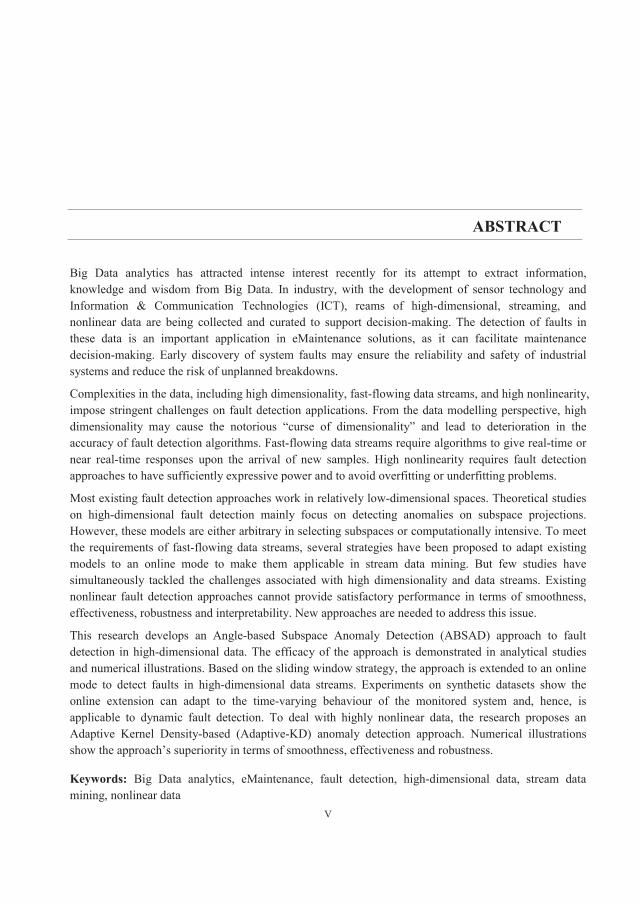
Big Data analytics has attracted intense interest recently for its attempt to extract information, knowledge and wisdom from Big Data. In industry, with the development of sensor technology and Information & Communication Technologies (ICT), reams of high-dimensional, streaming, and nonlinear data are being collected and curated to support decision-making. The detection of faults in these data is an important application in eMaintenance solutions, as it can facilitate maintenance decision-making. Early discovery of system faults may ensure the reliability and safety of industrial systems and reduce the risk of unplanned breakdowns.
Complexities in the data, including high dimensionality, fast-flowing data streams, and high nonlinearity, impose stringent challenges on fault detection applications. From the data modelling perspective, high dimensionality may cause the notorious “curse of dimensionality” and lead to deterioration in the accuracy of fault detection algorithms. Fast-flowing data streams require algorithms to give real-time or near real-time responses upon the arrival of new samples. High nonlinearity requires fault detection approaches to have sufficiently expressive power and to avoid overfitting or underfitting problems.
Most existing fault detection approaches work in relatively low-dimensional spaces. Theoretical studies on high-dimensional fault detection mainly focus on detecting anomalies on subspace projections. However, these models are either arbitrary in selecting subspaces or computationally intensive. To meet the requirements of fast-flowing data streams, several strategies have been proposed to adapt existing models to an online mode to make them applicable in stream data mining. But few studies have simultaneously tackled the challenges associated with high dimensionality and data streams. Existing nonlinear fault detection approaches cannot provide satisfactory performance in terms of smoothness, effectiveness, robustness and interpretability. New approaches are needed to address this issue.
This research develops an Angle-based Subspace Anomaly Detection (ABSAD) approach to fault detection in high-dimensional data. The efficacy of the approach is demonstrated in analytical studies and numerical illustrations. Based on the sliding window strategy, the approach is extended to an online mode to detect faults in high-dimensional data streams. Experiments on synthetic datasets show the online extension can adapt to the time-varying behaviour of the monitored system and, hence, is applicable to dynamic fault detection. To deal with highly nonlinear data, the research proposes an Adaptive Kernel Density-based (Adaptive-KD) anomaly detection approach. Numerical illustrations show the approach’s superiority in terms of smoothness, effectiveness and robustness.
Keywords: Big Data analytics, eMaintenance, fault detection, high-dimensional data, stream data mining, nonlinear data

VI

VII
LIST OF APPENDED PAPERS
Paper I Zhang, L., Lin, J. and Karim, R., 2015. An Angle-based Subspace Anomaly Detection Approach to
High-dimensional Data: With an Application to Industrial Fault Detection. Reliability Engineering &
System Safety, 142, pp.482-497.
Paper II
Zhang, L., Lin, J. and Karim, R., 2016. Sliding Window-based Fault Detection from High-dimensional Data Streams. IEEE Transactions on Systems, Man, and Cybernetics: System, Published online.
Paper III
Zhang, L., Lin, J. and Karim, R., 2016. Adaptive Kernel Density-based Anomaly Detection for Nonlinear Systems. Submitted to a journal.

VIII

IX
ACRONYMS
ABOD Angle-Based Outlier Detection ABSAD Angle-Based Subspace Anomaly Detection Adaptive-KD Adaptive Kernel Density ANN Artificial Neural Network AUC Area Under Curve CBM Condition-Based Maintenance CM Corrective Maintenance CMS Condition Monitoring System DFS Distributed File System D/I/K/I Data, Information, Knowledge, and Intelligence DISD Data-Intensive Scientific Discovery DSMS Data Stream Management System EAM Enterprise Asset Management ELM Extreme Learning Machine ERP Enterprise Resource Planning EWPCA Exponentially Weighted Principal Component Analysis FCM Fuzzy C-Means FD Fault Detection FDD Fault Detection and Diagnosis FPR False Positive Rate GMM Gaussian Mixture Model HALT Highly Accelerated Life Testing ICA Independent Component Analysis ICT Information & Communication Technologies KDE Kernel Density Estimate KICA Kernel Independent Component Analysis KPCA Kernel Principal Component Analysis LCC Life Cycle Cost LDA Linear Discriminant Analysis

X
LOF Local Outlier Factor LOS Local Outlier Score MIS Management Information System MPP Massively Parallel Processing MSPC Multivariate Statistical Process Control MTBD Mean Time Between Degradation MTBF Mean Time Between Failure NOSQL Not Only SQL NLP Natural Language Processing OEM Original Equipment Manufacturer OLAP Online Analytical Processing OLTP Online Transactional Processing OSA-CBM Open System Architecture for Condition-Based Maintenance PCA Principal Component Analysis PM Preventive Maintenance RAM Random Access Memory RDBMS Relational Database Management System ROC Receiver Operating Characteristic RPCA Recursive Principal Component Analysis RQ Research Question RUL Remaining Useful Life SCADA Supervisory Control And Data Acquisition SIS Safety Instrumented System SNN Shared Nearest Neighbours SOD Subspace Outlier Detection SOM Self-Organizing Map SPE Squared Prediction Error SQL Structured Query Language SVDD Support Vector Data Description SVM Support Vector Machine SWPCA Sliding Window Principal Component Analysis TBM Time-Based Maintenance TPR True Positive Rate XML Extensible Markup Language

XI
CONTENTS
CHAPTER 1. INTRODUCTION ............................................................................................................. 1
1.1 Background .................................................................................................................................. 1
1.1.1 Evolvement of maintenance strategy ........................................................................................ 2
1.1.2 Condition-based maintenance ................................................................................................... 4
1.2 Problem statement ........................................................................................................................ 7
1.3 Purpose and objectives ................................................................................................................. 8
1.4 Research questions ....................................................................................................................... 9
1.5 Linkage of research questions and appended papers ................................................................... 9
1.6 Scope and limitations ................................................................................................................... 9
1.7 Authorship of appended papers .................................................................................................. 10
1.8 Outline of thesis ......................................................................................................................... 10
CHAPTER 2. THEORETICAL FRAMEWORK .................................................................................. 13
2.1 Fault detection in eMaintenance ................................................................................................ 13
2.2 Big Data and Big Data analytics ................................................................................................ 14
2.3 “Curse of dimensionality” .......................................................................................................... 19
2.4 Stream data mining ..................................................................................................................... 20
2.5 Modelling with nonlinear data ................................................................................................... 21
2.6 Fault detection modelling ........................................................................................................... 23
2.6.1 Taxonomy of fault detection techniques ................................................................................ 23
2.6.2 Fault detection in high-dimensional data ................................................................................ 28
2.6.3 Fault detection in data streams ............................................................................................... 29
2.6.4 Fault detection in nonlinear data ............................................................................................ 30
2.7 Summary of framework ............................................................................................................. 32
CHAPTER 3. RESEARCH METHODOLOGY .................................................................................... 35
XII
3.1 Research design .......................................................................................................................... 35
3.2 Data generation and collection ................................................................................................... 37
3.2.1 Synthetic data generation ........................................................................................................ 37
3.2.2 Sensor data collection ............................................................................................................. 39
3.3 Data analysis .............................................................................................................................. 40
CHAPTER 4. RESULTS AND DISCUSSION ..................................................................................... 43
4.1 Results and discussion related to RQ 1 ...................................................................................... 43
4.1.1 Validation using synthetic datasets ......................................................................................... 43
4.1.2 Verification using a real-world dataset ................................................................................... 45
4.2 Results and discussion related to RQ 2 ...................................................................................... 46
4.2.1 Parameter tuning and analysis ................................................................................................ 47
4.2.2 Accuracy comparison and analysis ......................................................................................... 49
4.3 Results and discussion related to RQ 3 ...................................................................................... 51
4.3.1 Smoothness test using the “aggregation” dataset ................................................................... 52
4.3.2 Effectiveness test using a highly nonlinear dataset: a two-dimensional toroidal helix .......... 54
4.3.3 Robustness test using the “flame” dataset .............................................................................. 55
4.3.4 Verification using a real-world dataset ................................................................................... 57
4.3.5 Time complexity analysis ....................................................................................................... 59
CHAPTER 5. CONCLUSIONS, CONTRIBUTIONS AND FUTURE RESEARCH ........................... 61
5.1 Conclusions ................................................................................................................................ 61
5.2 Research contributions ............................................................................................................... 62
5.3 Future research ........................................................................................................................... 62
REFERENCES ......................................................................................................................................... 65

1
CHAPTER 1. INTRODUCTION This chapter describes the research area; it gives the problem statement, purpose and objectives, and research questions of the thesis, and explains its scope, limitations, and structure.
1.1 Background The widespread use of Information and Communication Technologies (ICT) has led to the advent of Big Data. In industry, unprecedented rates and scales of data are being generated from a wide array of sources, including sensor-intensive Condition Monitoring Systems (CMS), Enterprise Asset Management (EAM) systems, and Supervisory Control and Data Acquisition (SCADA) systems. They represent a rapidly expanding resource for operation and maintenance research, especially as researchers and practitioners are realizing the potential of exploiting hidden value from these data.
Figure 1.1: Integration of eMaintenance, e-Manufacturing and e-Business systems (Koc & Lee
2003; Kajko-Mattsson et al. 2011)
According to a recent McKinsey Institute report, the manufacturing industry is one of the five major domains where Big Data analytics can have transformative potential (Manyika et al. 2011). As a sub-concept of e-Manufacturing (Koc & Lee 2003), eMaintenance is also reaping benefits from Big Data analytics (Figure 1.1 illustrates the integration of eMaintenance, e-Manufacturing and e-Business systems). One of the major purposes of eMaintenance is to support maintenance decision-making.
eMaintenanceReal-time
dataCondition-based
MonitoringPredictive
TechnologiesInformation
Pipeline
VMIOutsourcing
CollaborativePlanningTechnology
Infrastructure
Real-time Information
Asset Management
e-Manufacturing
e-BusinessSCMTechnology
Infrastructure
CRM
e-Procurement
Trading Exchanges
Dynamic Decision Making
Background
2
Through the “e” of eMaintenance, the pertinent data, information, knowledge and intelligence (D/I/K/I) become available and usable at the right place and at the right time to make the right maintenance decisions all along the asset life cycle (Levrat et al. 2008). This is in line with the purpose of Big Data analytics, which is to extract information, knowledge, and wisdom from Big Data.
Although applying Big Data analytics to maintenance decision-making seems promising, the collected data tend to be high-dimensional, fast-flowing, unstructured, heterogeneous and complex (as will be detailed in Chapter 2) (Zhang & Karim 2014), thus posing significant challenges to existing data processing and analysis techniques. New forms of methods and technologies are required to analyse and process these data. This need has motivated the development of Big Data analytics in this thesis. To cite (Jagadish et al. 2014): “While the potential benefits of Big Data are real and significant, and some initial successes have already been achieved, there remain many technical challenges that must be addressed to fully realize this potential.”
1.1.1 Evolvement of maintenance strategy
The growing data deluge has fostered “the fourth paradigm” in scientific research, namely Data-Intensive Scientific Discovery (DISD) (Bell et al. 2009; Chen & Zhang 2014). The shift from empirical science (i.e., describing natural phenomena with empirical evidence), theoretical science (i.e., modelling of reality based on first principles), computational science (i.e., simulating complex phenomena using computers) to DISD has been witnessed in various scientific disciplines. In maintenance research, a similar transition can be seen in maintenance strategies, as shown in Figure 1.2.
Simply stated, maintenance research has evolved with the gradual replacement of Corrective Maintenance (CM) with Preventive Maintenance (PM) (Ahmad & Kamaruddin 2012). The oldest CM practices follow a “fail and fix” philosophy. This reactive strategy may result in unscheduled shutdowns and lead to significant economic loss or severe risks in safety and environmental aspects. The fear of shutdowns and their consequences motivated companies to perform maintenance and repair before asset failure, i.e., to adopt a PM strategy. PM suggests maintenance actions either based on a predetermined schedule (e.g., calendar time or the usage time of equipment) or the health condition of the equipment. The former is called Predetermined Maintenance, or Time-Based Maintenance (TBM), and the latter is Condition-Based Maintenance (CBM) (Ahmad & Kamaruddin 2012). In the early stages of PM development, maintenance activities were typically performed at fixed time intervals. The PM intervals were based on the knowledge of experienced technicians and engineers; the two major limitations of the approach were inefficiency and subjectivity. Another way of determining PM intervals is by following the Original Equipment Manufacturer (OEM) recommendations. OEM recommendations are based on laboratory experiments and reliability theory, such as Highly Accelerated Life Testing (HALT). With the arrival of advanced computing techniques, computational simulations of complex systems have also been used to recommend PM intervals (Percy & Kobbacy 2000).

INTRODUCTION
3
Figure 1.2: Maintenance strategies (CEN 2010)
Although unexpected failures can be greatly reduced with a predetermined maintenance strategy, there are two major problems. First, it tends to maintain equipment excessively, causing high maintenance costs (Peng et al. 2010). It seems paradoxical, but excessive maintenance may not necessarily improve the dependability of equipment; instead, it could even lead to more failures. Studies have shown that 50 to 70 percent of all equipment fails prematurely after maintenance is carried out (Karim et al. 2009). Second, it assumes the failure behaviour or characteristic is predictable. In other words, it presumes that equipment deteriorates deterministically following a well-defined sequence. Unfortunately, the assumption is not reflected in reality where failure behaviour is normally a function of equipment aging, environmental effects, process drifting, complex interactions between components and systems, and many other factors (Kothamasu et al. 2009). Several independent studies across industries have also indicated that 80 to 85 percent of equipment failures are caused by the effects of random events (Amari et al. 2006).
In general, CM strategy is prone to “insufficient maintenance”, while predetermined maintenance tends towards “excessive maintenance”. To solve the problem, a CBM strategy, or predictive maintenance, was proposed. CBM predicts future failures based on the health condition of equipment and initiates when maintenance tasks are needed. The primary difference between predetermined maintenance and CBM is that the maintenance activities of the latter are determined adaptively based on condition data. To capture the dynamically changing condition of equipment, vast amounts of data need to be measured and collected via condition monitoring, in-situ inspection or testing. Then, various data analysis techniques (e.g., machine learning, data mining, etc.) can be applied to assess the health condition of the equipment, thereby facilitating maintenance decision-making.
The evolution of maintenance strategy represents a considerable shift from reactivity to proactivity. It mirrors the above mentioned transition towards the DISD paradigm in scientific research. It was enabled by theoretical advances in maintenance management and developments in e-technologies. The concept
Maintenance
Preventive Maintenance Corrective Maintenance
Condition Based Maintenance
Deferred ImmediateScheduledScheduled, on request or continuous
Predetermined Maintenance
Background
4
eMaintenance uses e-technologies to support a shift from “fail and fix” maintenance practices to “prevent and predict” ones (Iung & Marquez 2006). In other words, it represents a transformation from the current Mean Time Between Failure (MTBF) practices to Mean Time Between Degradation (MTBD) practices (Iung & Marquez 2006).
1.1.2 Condition-based maintenance
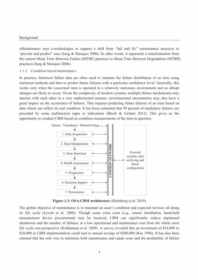
In practice, historical failure data are often used to estimate the failure distribution of an item using statistical methods and then to predict future failures with a particular confidence level. Generally, this works only when the concerned item is operated in a relatively stationary environment and no abrupt changes are likely to occur. Given the complexity of modern systems, multiple failure mechanisms may interact with each other in a very sophisticated manner; environmental uncertainties may also have a great impact on the occurrence of failures. This requires predicting future failures of an item based on data which can reflect its real condition. It has been estimated that 99 percent of machinery failures are preceded by some malfunction signs or indications (Bloch & Geitner 2012). This gives us the opportunity to conduct CBM based on condition measurements of the item in question.
Figure 1.3: OSA-CBM architecture (Holmberg et al. 2010)
The global objective of maintenance is to maintain an asset’s condition and expected services all along its life cycle (Levrat et al. 2008). Though some extra costs (e.g., sensor installation, hand-held measurement device procurement) may be incurred, CBM can significantly reduce unplanned shutdowns and the number of failures, at a low operational and maintenance cost from the whole asset life cycle cost perspective (Kothamasu et al. 2009). A survey revealed that an investment of $10,000 to $20,000 in CBM implementation could lead to annual savings of $500,000 (Rao 1996). It has also been claimed that the only way to minimize both maintenance and repair costs and the probability of failure
1. Data Acquisition
2. Data Manipulation
3. State Detection
4. Health Assessment
5. Prognostics
6. Decision Support
7. Presentation
Sensor / Transducer / Manual Entry
External systems, data archiving and
block configuration
CO
MM
ON
NE
TW
OR
K
INTRODUCTION
5
occurrence is to perform online system health monitoring and ongoing predictions of future failures (Kothamasu et al. 2009).
Formally, CBM is a type of preventive maintenance which includes a combination of condition monitoring and/or inspection and/or testing, analysis and the ensuing maintenance actions (CEN 2010). Condition monitoring, inspection, and testing are the main component of a CBM implementation. They can be conducted continuously, periodically or on request, depending on the criticality of the monitored item. The subsequent analysis assesses the health condition and predicts the Remaining Useful Life (RUL) of the item; this constitutes the core of a CBM scheme. The final step – determining maintenance actions – involves a maintenance decision-making process which considers maintenance resources, operational contexts, and inputs from other systems.
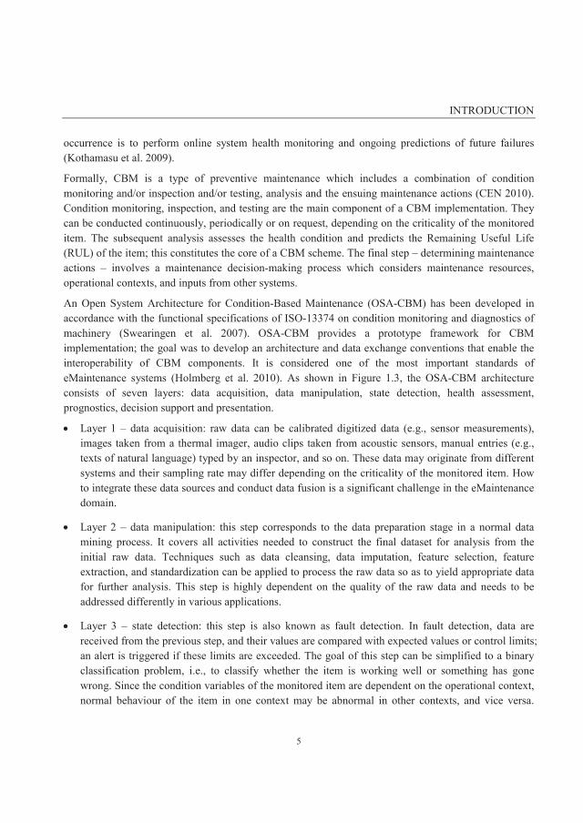
An Open System Architecture for Condition-Based Maintenance (OSA-CBM) has been developed in accordance with the functional specifications of ISO-13374 on condition monitoring and diagnostics of machinery (Swearingen et al. 2007). OSA-CBM provides a prototype framework for CBM implementation; the goal was to develop an architecture and data exchange conventions that enable the interoperability of CBM components. It is considered one of the most important standards of eMaintenance systems (Holmberg et al. 2010). As shown in Figure 1.3, the OSA-CBM architecture consists of seven layers: data acquisition, data manipulation, state detection, health assessment, prognostics, decision support and presentation.
Layer 1 – data acquisition: raw data can be calibrated digitized data (e.g., sensor measurements), images taken from a thermal imager, audio clips taken from acoustic sensors, manual entries (e.g., texts of natural language) typed by an inspector, and so on. These data may originate from different systems and their sampling rate may differ depending on the criticality of the monitored item. How to integrate these data sources and conduct data fusion is a significant challenge in the eMaintenance domain.
Layer 2 – data manipulation: this step corresponds to the data preparation stage in a normal data mining process. It covers all activities needed to construct the final dataset for analysis from the initial raw data. Techniques such as data cleansing, data imputation, feature selection, feature extraction, and standardization can be applied to process the raw data so as to yield appropriate data for further analysis. This step is highly dependent on the quality of the raw data and needs to be addressed differently in various applications.
Layer 3 – state detection: this step is also known as fault detection. In fault detection, data are received from the previous step, and their values are compared with expected values or control limits; an alert is triggered if these limits are exceeded. The goal of this step can be simplified to a binary classification problem, i.e., to classify whether the item is working well or something has gone wrong. Since the condition variables of the monitored item are dependent on the operational context, normal behaviour of the item in one context may be abnormal in other contexts, and vice versa.

Background
6
Therefore, fault detection procedures should be aware of changes in operational context and be adaptive to new operational environments.
Layer 4 – health assessment: this step focuses on determining if the health of a monitored item is degraded. If the health is degraded, a diagnosis on the faulty condition with an associated confidence level is needed. Concretely, health assessment consists of actions taken for fault recognition, fault localization, and identification of causes. The diagnosis procedure should be able to identify “what went wrong” (kind, situation and extent of the fault) as a further investigation of the fact that “something went wrong” derived at the previous step. A health assessment should also consider trends in health history, operational context and maintenance history.
Layer 5 – prognostics: this step projects the states of the monitored item into the future using a combination of prognostic models and future operational usage models. In other words, it estimates the RUL of the item taking into account the future operational utilization plan and other factors that could possibly affect the RUL. A confidence level of the assessment should also be given to represent the uncertainty in the RUL estimates.
Layer 6 – decision support: this step generates recommended actions based on the predictions of the future states of the item, current and future mission profiles, high-level unit objectives and resource constraints. The recommended actions may be operational or maintenance related. The former are typically straightforward, such as notification of alerts and the subsequent operating procedures. In the case of the latter, maintenance advisories need to be detailed enough to schedule maintenance activities in advance, such as the amount of required maintenance personnel, spare parts, tools and external services.
Layer 7 – presentation: this step provides an interactive human machine interface that facilitates analysis by qualified personnel. All the pertinent data, information and results obtained in previous steps should be connected through the network and visually presented in this layer. In some cases, analysts may need the ability to drill down from these results to get deeper insights.
The OSA-CBM architecture provides a holistic view of CBM. Each layer requires unique treatment, and different techniques have been developed specifically for each layer. Normally, the tasks defined in these layers should be sequentially and completely carried out to automatically schedule condition-based maintenance tasks. But in some cases, because of a lack of knowledge in some specific layers, the continuity of this sequentially linked chain is not guaranteed. For example, if there are no appropriate prognostic models, the prognosis task cannot be automatically performed. Under such circumstances, expert knowledge and experience can always be employed to complete the succeeding procedures. The preceding procedures can still be informative and provide a strong factual basis for human judgments (Vaidya & Rausand 2011). In this example, the procedures from layer 1 to layer 4 form the fault detection and diagnosis (FDD) application. Tasks from layer 1 to layer 3 comprise the fault detection (FD) application, the main research area in this thesis.
INTRODUCTION
7
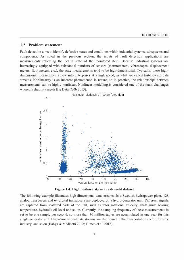
1.2 Problem statement Fault detection aims to identify defective states and conditions within industrial systems, subsystems and components. As noted in the previous section, the inputs of fault detection applications are measurements reflecting the health state of the monitored item. Because industrial systems are increasingly equipped with substantial numbers of sensors (thermometers, vibroscopes, displacement meters, flow meters, etc.), the state measurements tend to be high-dimensional. Typically, these high-dimensional measurements flow into enterprises at a high speed, in what are called fast-flowing data streams. Nonlinearity is an inherent phenomenon in nature, so in practice, the relationships between measurements can be highly nonlinear. Nonlinear modelling is considered one of the main challenges wherein reliability meets Big Data (Göb 2013).
Figure 1.4: High nonlinearity in a real-world dataset
The following example illustrates high-dimensional data streams. In a Swedish hydropower plant, 128 analog transducers and 64 digital transducers are deployed on a hydro-generator unit. Different signals are captured from scattered parts of the unit, such as rotor rotational velocity, shaft guide bearing temperature, hydraulic oil level and so on. Currently, the sampling frequency of these measurements is set to be one sample per second, so more than 30 million tuples are accumulated in one year for this single generator unit. High-dimensional data streams are also found in the transportation sector, forestry industry, and so on (Bahga & Madisetti 2012; Fumeo et al. 2015).
Purpose and objectives
8
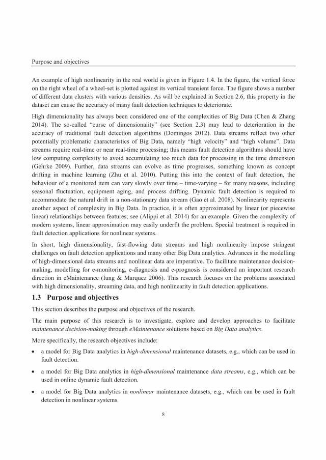
An example of high nonlinearity in the real world is given in Figure 1.4. In the figure, the vertical force on the right wheel of a wheel-set is plotted against its vertical transient force. The figure shows a number of different data clusters with various densities. As will be explained in Section 2.6, this property in the dataset can cause the accuracy of many fault detection techniques to deteriorate.
High dimensionality has always been considered one of the complexities of Big Data (Chen & Zhang 2014). The so-called “curse of dimensionality” (see Section 2.3) may lead to deterioration in the accuracy of traditional fault detection algorithms (Domingos 2012). Data streams reflect two other potentially problematic characteristics of Big Data, namely “high velocity” and “high volume”. Data streams require real-time or near real-time processing; this means fault detection algorithms should have low computing complexity to avoid accumulating too much data for processing in the time dimension (Gehrke 2009). Further, data streams can evolve as time progresses, something known as concept drifting in machine learning (Zhu et al. 2010). Putting this into the context of fault detection, the behaviour of a monitored item can vary slowly over time – time-varying – for many reasons, including seasonal fluctuation, equipment aging, and process drifting. Dynamic fault detection is required to accommodate the natural drift in a non-stationary data stream (Gao et al. 2008). Nonlinearity represents another aspect of complexity in Big Data. In practice, it is often approximated by linear (or piecewise linear) relationships between features; see (Alippi et al. 2014) for an example. Given the complexity of modern systems, linear approximation may easily underfit the problem. Special treatment is required in fault detection applications for nonlinear systems.
In short, high dimensionality, fast-flowing data streams and high nonlinearity impose stringent challenges on fault detection applications and many other Big Data analytics. Advances in the modelling of high-dimensional data streams and nonlinear data are imperative. To facilitate maintenance decision-making, modelling for e-monitoring, e-diagnosis and e-prognosis is considered an important research direction in eMaintenance (Iung & Marquez 2006). This research focuses on the problems associated with high dimensionality, streaming data, and high nonlinearity in fault detection applications.
1.3 Purpose and objectives This section describes the purpose and objectives of the research.
The main purpose of this research is to investigate, explore and develop approaches to facilitate maintenance decision-making through eMaintenance solutions based on Big Data analytics.
More specifically, the research objectives include:
a model for Big Data analytics in high-dimensional maintenance datasets, e.g., which can be used in fault detection.
a model for Big Data analytics in high-dimensional maintenance data streams, e.g., which can be used in online dynamic fault detection.
a model for Big Data analytics in nonlinear maintenance datasets, e.g., which can be used in fault detection in nonlinear systems.
INTRODUCTION
9
1.4 Research questions To achieve the stated purpose and objectives, the following research questions have been formulated:
RQ 1: How can patterns be extracted from maintenance Big Data with high dimensionality characteristics?
RQ 2: How should high-dimensional data streams be dealt with in the analysis of maintenance Big Data?
RQ 3: How should nonlinearity be dealt with in the analysis of maintenance Big Data?
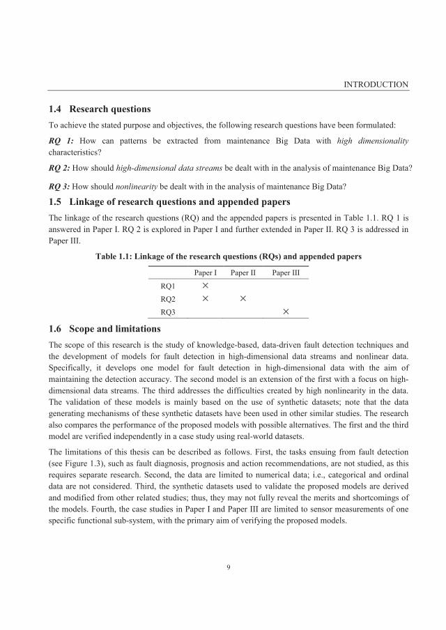
1.5 Linkage of research questions and appended papers The linkage of the research questions (RQ) and the appended papers is presented in Table 1.1. RQ 1 is answered in Paper I. RQ 2 is explored in Paper I and further extended in Paper II. RQ 3 is addressed in Paper III.
Table 1.1: Linkage of the research questions (RQs) and appended papers
Paper I Paper II Paper III
RQ1
RQ2
RQ3
1.6 Scope and limitations The scope of this research is the study of knowledge-based, data-driven fault detection techniques and the development of models for fault detection in high-dimensional data streams and nonlinear data. Specifically, it develops one model for fault detection in high-dimensional data with the aim of maintaining the detection accuracy. The second model is an extension of the first with a focus on high-dimensional data streams. The third addresses the difficulties created by high nonlinearity in the data. The validation of these models is mainly based on the use of synthetic datasets; note that the data generating mechanisms of these synthetic datasets have been used in other similar studies. The research also compares the performance of the proposed models with possible alternatives. The first and the third model are verified independently in a case study using real-world datasets.
The limitations of this thesis can be described as follows. First, the tasks ensuing from fault detection (see Figure 1.3), such as fault diagnosis, prognosis and action recommendations, are not studied, as this requires separate research. Second, the data are limited to numerical data; i.e., categorical and ordinal data are not considered. Third, the synthetic datasets used to validate the proposed models are derived and modified from other related studies; thus, they may not fully reveal the merits and shortcomings of the models. Fourth, the case studies in Paper I and Paper III are limited to sensor measurements of one specific functional sub-system, with the primary aim of verifying the proposed models.

Authorship of appended papers
10
1.7 Authorship of appended papers The contribution of each author to the appended papers with respect to the following activities is shown in Table 1.2:
1. Formulating the fundamental ideas of the problem;
2. Performing the study;
3. Drafting the paper;
4. Revising important intellectual contents;
5. Giving final approval for submission.
Table 1.2: Contribution of the authors to the appended papers (I-III)
Paper I Paper II Paper III Liangwei Zhang 1-5 1-5 1-5 Jing Lin 1,4,5 1,4,5 1,4,5 Ramin Karim 1,4,5 1,4,5 1,4,5
1.8 Outline of thesis The thesis consists of five chapters and three appended papers:
Chapter 1 – Introduction: the chapter gives the area of research, the problem definition, the purpose and objectives of the thesis, the research questions, the linkage between the research questions and the appended papers, the scope and limitations of the research, and the authorship of appended papers.
Chapter 2 – Theoretical framework: the chapter provides the theoretical framework for the research. Most of the chapter focuses on existing fault detection techniques and challenges posed by high-dimensional data, fast-flowing and non-stationary data streams, and high nonlinearity in the data.
Chapter 3 – Research methodology: the chapter systematically describes how the research was conducted.
Chapter 4 – Results and discussion: the chapter presents the results and a discussion of the research corresponding to each of the research questions.
Chapter 5 – Conclusions, contributions and future research: this chapter concludes the work, synthesizes the contribution of the thesis and suggests future research.
Paper I proposes an Angle-based Subspace Anomaly Detection (ABSAD) approach to fault detection in high-dimensional data. The aim is to maintain detection accuracy in high-dimensional circumstances. To comprehensively compare the proposed model with several other alternatives, artificial datasets with various high-dimensional settings are constructed. Results show the superior accuracy of the model. A

INTRODUCTION
11
further experiment using a real-world dataset demonstrates the applicability of the proposed model in fault detection tasks.
Paper II extends the model proposed in Paper I to an online mode with the aim of detecting faults from non-stationary, high-dimensional data streams. It also proposes a two-stage fault detection scheme based on the sliding window strategy. The efficacy of the online ABSAD model is demonstrated by means of synthetic datasets and comparisons with possible alternatives. The results of the experiments show the proposed model can be adaptive to the time-varying behaviour of a monitored item.
Paper III proposes an Adaptive Kernel Density-based (Adaptive-KD) anomaly detection approach to fault detection in nonlinear data. The purpose is to define a smooth yet effective measure of outlierness that can be used to detect anomalies in nonlinear systems. The model is extended to an online mode to deal with stationary data streams. For validation, the model is compared to several alternatives using both synthetic and real-world datasets; the model displays superior efficacy in terms of smoothness, effectiveness and robustness.

12
13
CHAPTER 2. THEORETICAL FRAMEWORK This chapter presents the theoretical framework of this research. The goal is to review the theoretical basis of the thesis and provide a context for the appended papers. The literature sources cited herein include conference proceedings, journals, international standards, and other indexed publications.
2.1 Fault detection in eMaintenance Maintenance refers to a combination of all technical, administrative and managerial actions during the life cycle of an item intended to retain it in, or restore it to, a state in which it can perform the required function (CEN 2010). eMaintenance is defined as a multidisciplinary domain based on the use of maintenance and information and communication technologies to ensure maintenance services are aligned with the needs and business objectives of both customers and suppliers during the whole product life cycle (Kajko-Mattsson et al. 2011). It has also been considered a maintenance management concept whereby assets are monitored and managed over the Internet (Iung & Marquez 2006). In addition, it can be seen as a philosophy to support the transition from corrective maintenance practices to preventive maintenance strategies, i.e., from reactivity to proactivity; the key to realizing this transition is to implement e-monitoring to monitor system health, i.e., CBM.
In CBM, the health of equipment is monitored based on its operating conditions, and maintenance activities are recommended based on predictions of future failures. A properly implemented CBM program can significantly reduce maintenance costs by reducing the number of unnecessary scheduled PM actions (Jardine et al. 2006). It is also important for better equipment health management, lower asset life cycle cost, the avoidance of catastrophic failure, and so on (Rosmaini & Kamaruddin 2012).
According to the standard ISO-13374 and the OSA-CBM architecture (see Subsection 1.1.2), fault detection is an indispensable element of a CBM system. It can provide informative knowledge for the ensuing procedures, including fault diagnosis, prognosis and action recommendations.
Fault detection intends to identify defective states and conditions within industrial systems, subsystems and components. Early discovery of system faults may ensure the reliability and safety of industrial systems and reduce the risk of unplanned breakdowns (Dai & Gao 2013; Zhong et al. 2014). Fault detection is a vital component of an Integrated Systems Health Management system; it is also considered one of the most promising applications wherein reliability meets Big Data (Meeker & Hong 2014). In
Big Data and Big Data analytics
14
practice, fault detection can be separated from the OSA-CBM architecture and serve as a stand-alone application to support maintenance decision-making and eMaintenance. At the same time, eMaintenance as a framework may provide other related data, information and knowledge to a fault detection system. For example, as mentioned earlier, a fault detection system should be aware of the operational context of the monitored system and be adaptive to any changes in the context. In this scenario, an integrated eMaintenance platform can facilitate the information exchange between different systems. In short, fault detection is one way to approach eMaintenance, as its integrated architecture and platform support fault detection.
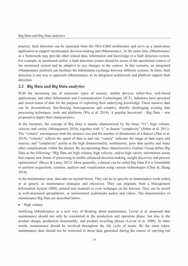
2.2 Big Data and Big Data analytics With the increasing use of numerous types of sensors, mobile devices, tether-free, web-based applications, and other Information and Communication Technologies (ICT), industries have procured and stored reams of data for the purpose of exploiting their underlying knowledge. These massive data can be decentralized, fast-flowing, heterogeneous and complex, thereby challenging existing data processing techniques, tools and platforms (Wu et al. 2014). A popular buzzword – Big Data – was proposed to depict their characteristics.
In the literature, the concept of Big Data is mainly characterized by the three “Vs”, high volume, velocity and variety (Montgomery 2014), together with “c” to denote “complexity” (Sribar et al. 2011). The “volume” encompasses both the instance size and the number of dimensions of a dataset (Zhai et al. 2014), “velocity” reflects the speed of data in and out, “variety” indicates the range of data types and sources, and “complexity” points to the high dimensionality, nonlinearity, poor data quality and many other complications within the dataset. By incorporating these characteristics, Gartner Group define Big Data as the following: “Big Data are high volume, high velocity, and/or high variety information assets that require new forms of processing to enable enhanced decision-making, insight discovery and process optimization” (Beyer & Laney 2012). More generally, a dataset can be called Big Data if it is formidable to perform acquisition, curation, analysis and visualization using current technologies (Chen & Zhang 2014).
In the maintenance area, data take on myriad forms. They can be as specific as maintenance work orders, or as generic as maintenance strategies and objectives. They can originate from a Management Information System (MIS), printed user manuals or even webpages on the Internet. They can be stored in well-structured spreadsheets, or unstructured multimedia audios and videos. The characteristics of maintenance Big Data are described below.
High volume
Justifying eMaintenance as a new way of thinking about maintenance, Levrat et al. proposed that maintenance should not only be considered in the production and operation phase, but also in the product design, production disassembly, and product recycling phases (Levrat et al. 2008). In other words, maintenance should be involved throughout the life cycle of assets. By the same token, maintenance data should not be restricted to those data generated during the course of carrying out
THEORETICAL FRAMEWORK
15
maintenance tasks. All the relevant data produced before and after maintenance tasks should be included in the range of maintenance data, as long as they contribute to maintenance work (Zhang & Karim 2014).
In accordance with the phases of the asset life cycle (PAS n.d.), maintenance data can be decomposed as follows. First, in the phase “creation, acquisition or enhancement of assets”, data, as for instance, the technical specifications provided by asset suppliers, can have a great impact on the formulation of maintenance strategies. For example, the recommended preventive maintenance interval should be considered a significant input to determine the frequency of implementing predetermined maintenance tasks. Other maintenance data produced in this phase include asset drawings, technical specification documentation, the number of attached spare parts, purchase contracts and warranty terms, etc. Second, in the phase “utilization of assets”, the asset utilization schedule may affect the implementation of maintenance work, and vice versa. For example, some maintenance tasks are implemented by opportunities presented when a partial or full stoppage of a process area occurs. Maintenance data produced in this phase include production scheduling, hazard and precaution identifications, environmental conditions, operating load and parameters, etc. Third, in the phase “maintenance of assets”, the great majority of maintenance data is generated. These data can be leveraged to support maintenance work. In this phase, maintenance data encompass condition-monitoring data, feedback from routine inspections, failure data, maintenance resources, work orders, overhaul and refurbishment plans, and so forth. Lastly, in the phase “decommissioning and/or disposal of assets”, maintenance is associated with financial accounting in terms of asset depreciation or scrapping. Therefore, maintenance data in this phase primarily consist of depreciation expenses and recycling information. Depreciation expenses should be taken into account in calculating the Life Cycle Cost (LCC) of an asset, while information on recycling a retiring asset needs to be recorded in case of any future investigations.
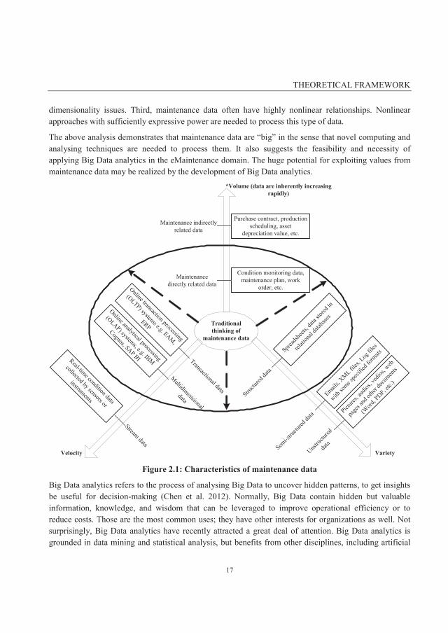
To facilitate maintenance decision-making by using eMaintenance, the range of maintenance data should be expanded to a broader scope, as shown in the volume dimension in Figure 2.1. Of course, the size of maintenance data has increased substantially in the last decade. With the aim of supporting different functionalities of operation and maintenance, various information systems are now deployed in industries. Among these systems, common ones include Enterprise Asset Management (EAM) system, Enterprise Resource Planning (ERP) system, Condition monitoring System (CMS), Supervisory Control and Data Acquisition (SCADA) system and Safety Instrumented System (SIS). These systems generate troves of maintenance data which need to be processed using Big Data technologies. To sum up, then, in the context of eMaintenance, high volume is a characteristic of maintenance Big Data.
High velocity
In current maintenance practices, Online Transactional Processing (OLTP) and Online Analytical Processing (OLAP) are the two major types of systems dealing with maintenance data (see the velocity dimension in Figure 2.1) (Göb 2013). The former ensures basic functionalities and performance of maintenance related systems (such as EAM) under concurrency, while the latter allows complicated analytical and ad hoc queries by introducing data redundancy in data cubes.
Big Data and Big Data analytics
16
For the purpose of condition-based maintenance, sensors and various measurement instruments are deployed on equipment, leading to the generation of high-speed maintenance data streams. Equipment anomalies indicated by those data streams should be addressed promptly; decisive actions are required to avoid unplanned breakdowns and economic losses. The OLTP and OLAP systems are designed for a specific purpose, however, and cannot process these fast-moving data streams efficiently.
Prompt analysis of data streams will facilitate maintenance decision-making by ensuring a faster response time. Organizations can seize opportunities in a dynamic and changing market, while avoiding operational and economic losses. Big Data analytics are needed in this context.
High variety
Maintenance data can be derived from wireless sensor networks, running log documents, surveillance image files, audio and video clips, complicated simulation and GPS-enabled spatiotemporal data, and much more. These types of maintenance data are becoming increasingly diverse, i.e., structured, semi-structured or unstructured (see the variety dimension in Figure 2.1).
Structured maintenance data are mostly stored in relational databases (such as Oracle, DB2, SQL Server, etc.). Most of the maintenance data curated in the aforementioned information systems are structured. From the perspective of data size, unstructured data are becoming dominant in the whole information available within an organization (Warren & Davies 2007). Examples of unstructured maintenance data include: technical documentation of equipment, images taken by infrared thermal imagers, frequency spectrums collected by vibration detection equipment, movement videos captured by high-speed digital cameras, etc. Semi-structured data fall between the above two data types. They are primarily text-based and conform to specified rules. Within semi-structured data, tags or other forms of markers are used to identify certain elements. Maintenance data belonging to this type comprise emails, XML files, and log files with specified formats.
In general, structured data can be easily accessed and manipulated by Structured Query Language (SQL). Conversely, unstructured and semi-structured data are relatively difficult to curate, categorize and analyse using traditional computing solutions (Chen & Zhang 2014). More Big Data technologies are needed to facilitate excavating patterns from these data and, hence, to support maintenance decision-making.
High complexity
Maintenance data are complex. They can take many different forms and may vary across industries. Examples of their complexity include the following. First, maintenance data quality can be poor; the data can be inaccurate (e.g., sensor data with environmental noise), uncertain (e.g., predictions of the remaining useful life of a critical component) and biased (e.g., intervals of time-based maintenance). The data quality problem is generally tackled by data quality assurance/control procedures and data cleaning techniques. Second, maintenance data can be high-dimensional. Advanced feature selection techniques, dimension reduction techniques and algorithms need to be developed to address the high
THEORETICAL FRAMEWORK
17
dimensionality issues. Third, maintenance data often have highly nonlinear relationships. Nonlinear approaches with sufficiently expressive power are needed to process this type of data.
The above analysis demonstrates that maintenance data are “big” in the sense that novel computing and analysing techniques are needed to process them. It also suggests the feasibility and necessity of applying Big Data analytics in the eMaintenance domain. The huge potential for exploiting values from maintenance data may be realized by the development of Big Data analytics.
Figure 2.1: Characteristics of maintenance data
Big Data analytics refers to the process of analysing Big Data to uncover hidden patterns, to get insights be useful for decision-making (Chen et al. 2012). Normally, Big Data contain hidden but valuable information, knowledge, and wisdom that can be leveraged to improve operational efficiency or to reduce costs. Those are the most common uses; they have other interests for organizations as well. Not surprisingly, Big Data analytics have recently attracted a great deal of attention. Big Data analytics is grounded in data mining and statistical analysis, but benefits from other disciplines, including artificial
*Volume (data are inherently increasing rapidly)
VarietyVelocity
Traditional thinking of
maintenance data
Transactional data
Online transaction processing
(OLTP) systems e.g. EAM,
ERP
Multidimensional
data
Online analytical processing
(OLAP) systems, e.g. IBM
Cognos, SAP BI
Structu
red da
ta
Spread
sheets
, data
stored
in
relati
onal
datab
ases
Semi-s
tructu
red da
ta
Emails, X
ML files,
Log fil
es
with so
me spe
cified
form
ats
Unstruc
tured
data
Picture
s, aud
ios, v
edios
, web
page
s and
othe
r doc
umen
ts
(Word
, PDF, e
tc.)
Stream data
Real-time condition data
collected by sensors or
instruments
Maintenance directly related data
Condition monitoring data, maintenance plan, work
order, etc.
Maintenance indirectly related data
Purchase contract, production scheduling, asset
depreciation value, etc.
Big Data and Big Data analytics
18
intelligence, signal processing, optimization methods and visualization approaches (Chen & Zhang 2014).
Each characteristic of Big Data (high volume, velocity, variety, and complexity) poses a unique challenge to Big Data analytics; the technologies designed to handle them are discussed below.
To handle the huge volume of Big Data, Distributed File Systems (DFS) have been developed to meet storage requirements, Massively Parallel Processing (MPP) systems have been devised to meet the demand of fast computing, and so forth (Chen & Zhang 2014). Notably, these technologies are targeted at overcoming the difficulties resulting from tremendous instance size. The other aspect of Big Data volume, high dimensionality, has received much less attention. A recent study highlighted this under-explored topic, “big dimensionality”, and appealed for more research efforts (Zhai et al. 2014).
High velocity refers to the high rate of data generation, also known as the data stream. Data streams must be processed in a real-time or near real-time manner. In other words, the ongoing data processing must have very low latency of response. To this end, a variety of stream processing tools have been developed, including Storm, Yahoo S4, SQLstream, Apache Kafka and SAP Hana (Chen & Zhang 2014). Among these stream-processing tools, several adopt the in-memory processing technology where the arriving data are loaded in Random Access Memory (RAM) instead of on disk drives. The use of in-memory processing technology is not limited to stream data mining. It has also been applied to other applications where fast responses are desired, such as the Apache Spark project (Apache n.d.). In addition to the development of stream processing tools, a large number of data mining techniques have been extended to an online mode for the purpose of stream data mining.
High variety alludes to the multitudinous formats of Big Data, i.e., structured, semi-structured and unstructured data. Structured data are consistently preserved in a well-defined schema and conform to some common standards, such as data stored in Relational Database Management Systems (RDBMS). Unstructured data refer to data without a predefined schema, such as noisy text, images, videos, audios. Semi-structured data are a cross between the other two types and have a relatively loose structure. The main challenge of this characteristic comes from the semi-structured and unstructured data. Extensible Markup Language (XML) has been designed to represent and process semi-structured data. NoSQL, i.e., not only SQL, databases have been developed to augment the flexibility of schema design and horizontal scalability (Chen & Zhang 2014). Data with less structure can be efficiently stored and accessed from NoSQL databases. Natural Language Processing (NLP) has been extensively studied during the past decade; several techniques, including normalization, stemming and lemmatization, feature extraction, etc., are now available for processing textual data. Image, audio and video processing have also been developed. Recently, a general method of learning from these unstructured data – deep learning – has attracted considerable attention (Zou et al. 2012).
High complexity includes high dimensionality, high nonlinearity, poor data quality, and many other properties of Big Data (Sribar et al. 2011). It can lead to significant security problems, suggesting the need for data security protection, intellectual property protection, personal privacy protection, and so
THEORETICAL FRAMEWORK
19
on. Taking high dimensionality as an example, several manifold learning techniques have been proposed to conduct dimensionality reduction, such as Locally Linear Embedding, ISOMAP (Tenenbaum et al. 2000; Roweis & Saul 2000). The complexity of Big Data is highly dependent on concrete applications. Each complexity presents a distinct challenge to Big Data analytics and needs to be addressed differently.
The hype surrounding Big Data and Big Data analytics has arguably stemmed from the web and e-commerce communities (Chen et al. 2012). But it is positively impacting other disciplines and benefits are reaped when Big Data technologies are adopted in those fields. In industry, mining from high-speed data streams and sensor data has recently been identified as one of the emerging research areas in Big Data analytics (Chen et al. 2012). The work in this thesis can be ascribed to this branch of research.
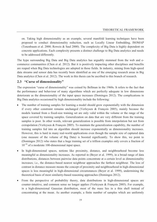
2.3 “Curse of dimensionality” The expression “curse of dimensionality” was coined by Bellman in the 1960s. It refers to the fact that the performance and behaviour of many algorithms which are perfectly adequate in low dimensions deteriorate as the dimensionality of the input space increases (Domingos 2012). The complications in Big Data analytics occasioned by high dimensionality include the following:
The number of training samples for learning a model should grow exponentially with the dimension if every other constraint remains unchanged (Verleysen & François 2005), mainly because the models learned from a fixed-size training set are only valid within the volume or the range of the space covered by training samples. Generalization on data that are very different from the training samples is poor. In other words, relevant generalization is possible from interpolation but not from extrapolation (Verleysen & François 2005). To maintain the generalization capability, the number of training samples fed into an algorithm should increase exponentially as dimensionality increases. However, this is hard in many real-world applications even though the sample size of captured data (one measure of the volume of Big Data) is boosted significantly. To show this, we point to (Domingos 2012) who states that a huge training set of a trillion examples only covers a fraction of 10-18 of a moderate 100-dimensional input space.
In high-dimensional spaces, notions like proximity, distance, and neighbourhood become less meaningful as dimensionality increases. As reported in (Beyer et al. 1999), in a broad range of data distributions, distances between pairwise data points concentrate at a certain level as dimensionality increases; i.e., the distance-based nearest neighbour approaches the farthest neighbour. The loss of contrast in distance measure means the concept of proximity and neighbourhood in high-dimensional spaces is less meaningful in high-dimensional circumstances (Beyer et al. 1999), undermining the theoretical basis of most similarity-based reasoning approaches (Domingos 2012).
From the perspective of probability theory, data distributions in high-dimensional spaces are counter-intuitive, and common sense no longer applies (Verleysen & François 2005). For example, in a high-dimensional Gaussian distribution, most of the mass lies in a thin shell instead of concentrating at the mean. As another example, a finite number of samples which are uniformly

Stream data mining
20
distributed in a high-dimensional hypercube tend to be closer to the surface of the hypercube than to their nearest neighbours. This phenomenon jeopardizes Big Data analytics in which algorithms are normally designed based on intuitions and examples in low-dimensional spaces (Verleysen & François 2005).
High dimensionality has been recognized as the distinguishing feature of modern field reliability data, i.e., periodically generated large vectors of dynamic covariate values (Meeker & Hong 2014). Because of the “curse of dimensionality”, it is also regarded as a primary complexity of multivariate analysis and covariate-response analysis in reliability applications (Göb 2013). Although numerous studies have sought to overcome the “curse of dimensionality” in different applications, high dimensionality is still acknowledged as one of the biggest challenges in Big Data analytics (Chen & Zhang 2014).
2.4 Stream data mining Data streams are becoming ubiquitous in the real world. The term refers to data continuously generated at a high rate. Normally, data streams are also temporally ordered, fast changing, and potentially infinite (Krawczyk et al. 2015; Olken & Gruenwald 2008). The properties of data streams reflect the characteristics of Big Data in the aspects of both high volume and high velocity. These fast, infinite and non-stationary data streams pose more challenges to Big Data analytics, as summarized by the following:
Stream data mining applications demand the implemented algorithm gives real-time or near real-time responses. For example, when assessing the health status of a system, the monitoring program must have low-latency in responding to the fast-flowing data streams. Therefore, “on-the-fly” analysis with low computational complexity is desired (Krawczyk et al. 2015).
Given the potentially infinite property of data streams, it is impractical or even impossible to scan a data stream multiple times considering the finite memory resources. Under these circumstances, one-pass algorithms that conduct one scan of the data stream are imperative (Olken & Gruenwald 2008). However, it is generally hard to achieve satisfactory accuracy while training the model with a constant amount of memory.
A data stream can evolve as time progresses. Concept drifting refers to changes in data generating mechanisms over time (Gao et al. 2008). For example, in the context of system health monitoring, the behaviour of systems can vary slowly over time – time-varying – for many reasons, such as seasonal fluctuation, equipment aging, process drifting, and so forth. The monitoring program must be able to adapt to the time-varying behaviour of the monitored system (Gao et al. 2008). A typical way to address concept drifting is by giving greater weight to information from the recent past than from the distant past.
Current research efforts on data stream processing focus on two aspects: systems and algorithms (Gehrke 2009). For the former, several data stream management systems (DSMS) have been developed to cater to the specific needs of data stream processing (see Section 2.2). For the latter, many algorithms have been extended from existing ones for the purposes of stream data mining. For example, the training of a logistic regression classifier can be transformed from a batch mode to an online mode using
THEORETICAL FRAMEWORK
21
stochastic gradient descent. This optimization technique takes a subset of samples from the training set and optimizes the loss function iteratively. More discussion of this appears in Subsection 2.6.3.
Notably, real-world data streams tend to be high-dimensional, e.g., sensor networks, cyber surveillance, and so on (Aggarwal et al. 2005). In academia, the challenges posed by high dimensional data streams are often addressed separately with respect to solving the problems of high dimensionality or performing stream data mining. On the one hand, several dimensionality reduction techniques have been employed in high-dimensional classification problems (Agovic et al. 2009). On the other hand, granularity-based techniques (such as sampling) have been devised to cope with the requirements of high-speed data streams (Gao et al. 2008). However, few studies simultaneously tackle the challenges associated with high dimensionality and data streams.
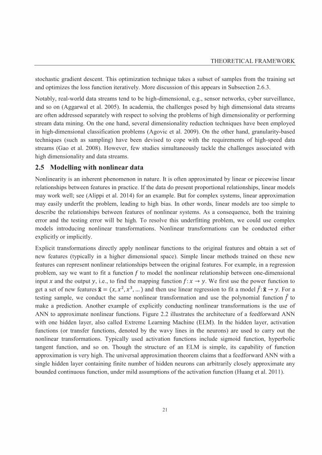
2.5 Modelling with nonlinear data Nonlinearity is an inherent phenomenon in nature. It is often approximated by linear or piecewise linear relationships between features in practice. If the data do present proportional relationships, linear models may work well; see (Alippi et al. 2014) for an example. But for complex systems, linear approximation may easily underfit the problem, leading to high bias. In other words, linear models are too simple to describe the relationships between features of nonlinear systems. As a consequence, both the training error and the testing error will be high. To resolve this underfitting problem, we could use complex models introducing nonlinear transformations. Nonlinear transformations can be conducted either explicitly or implicitly.
Explicit transformations directly apply nonlinear functions to the original features and obtain a set of new features (typically in a higher dimensional space). Simple linear methods trained on these new features can represent nonlinear relationships between the original features. For example, in a regression problem, say we want to fit a function to model the nonlinear relationship between one-dimensional input and the output , i.e., to find the mapping function : . We first use the power function to get a set of new features xx = ( , , , … ) and then use linear regression to fit a model : xx . For a testing sample, we conduct the same nonlinear transformation and use the polynomial function to make a prediction. Another example of explicitly conducting nonlinear transformations is the use of ANN to approximate nonlinear functions. Figure 2.2 illustrates the architecture of a feedforward ANN with one hidden layer, also called Extreme Learning Machine (ELM). In the hidden layer, activation functions (or transfer functions, denoted by the wavy lines in the neurons) are used to carry out the nonlinear transformations. Typically used activation functions include sigmoid function, hyperbolic tangent function, and so on. Though the structure of an ELM is simple, its capability of function approximation is very high. The universal approximation theorem claims that a feedforward ANN with a single hidden layer containing finite number of hidden neurons can arbitrarily closely approximate any bounded continuous function, under mild assumptions of the activation function (Huang et al. 2011).

Modelling with nonlinear data
22
Figure 2.2: Architecture of a feedforward ANN with a single hidden layer
Implicit transformations are typically used when inner-products between samples, i.e., , , appear in the problem formulation of linear methods. Under such circumstances, we can replace the inner product by a kernel function : , R, which maps the inner product between samples to a real domain. A valid kernel needs to satisfy Mercer’s condition which requires the function to be symmetric and the produced kernel matrix (or Gram matrix) to be positive semi-definite (Campbell 2002). Frequently used kernel functions include polynomial kernel, Gaussian kernel, sigmoid kernel, and many others. Both the inner product and the kernel function evaluation can be considered similarity measures between samples. Substituting the inner product with the kernel function enables the nonlinear transformation of the data points to an alternative high-dimensional (possibly infinite) feature space, i.e., , ( ), . Here, the functional form of the mapping ( ) does not need to be known because it is implicitly defined by the choice of the kernel function. This implicit transformation is often called “the kernel trick”, and it can greatly boost the ability of linear methods to deal with nonlinear data. Examples of approaches applying the kernel trick include Linear Discriminant Analysis (LDA), Support Vector Machine (SVM), Gaussian process, Principal Component Analysis (PCA), and many others.
Both the explicit and implicit transformations introduced above provide powerful mechanisms to model nonlinear data, but if the selected hyper-parameters are inappropriate, overfitting or underfitting problems could result. Intuitively, the overfitting problem implies the model is too complex to describe the relationships between features in nonlinear systems. The learned model can even explain the noise in the data. For instance, in the polynomial regression example, if the polynomial degree is large enough, the mapping function can fit perfectly to all the data in the training set, leading to zero empirical error. But the testing error could be remarkably high (high variance), indicating a poor generalization of the model. This problem is also common in those kernel methods which implicitly conduct nonlinear transformations.
x1 x2 xi xd
…... …... 1
1…... …...
Input layer
Hidden layer
Output layer
1y
…...2y ˆmy
THEORETICAL FRAMEWORK
23
Two commonly used techniques to address the overfitting problem are regularization or the addition of more representative data to the training set. Regularization penalizes the complexity and improves the generalization capability of a model; examples include ridge regression, auto encoders, dropout nets (Srivastava et al. 2014). Adding more representative data to the training set can alleviate the overfitting problem, but it could be expensive in some cases. Adding more representative data is often the primary choice in practice to improve the performance of a model, but in cases of underfitting, adding more data will not help. The ultimate goal for a learning model is to improve its generalization capability. How to select a model with a better tradeoff between overfitting and underfitting is an art in most real-world applications. Notably, some approaches naturally have the ability to deal with nonlinear data, such as density-based approaches. Later sections describe these in detail, with a focus on anomaly detection.
2.6 Fault detection modelling From the perspective of data modelling, fault detection can be considered anomaly detection or outlier detection. Anomaly detection aims to detect observations which deviate so much from others that they are suspected of being generated by different mechanisms (Hawkins 1980). It has been extensively applied in many fields, including cyber intrusion detection, financial fraud detection and so forth (Albaghdadi et al. 2006; Li et al. 2008). Hereinafter, we consider fault detection, anomaly detection, and outlier detection as interchangeable terms, unless otherwise stated.
2.6.1 Taxonomy of fault detection techniques
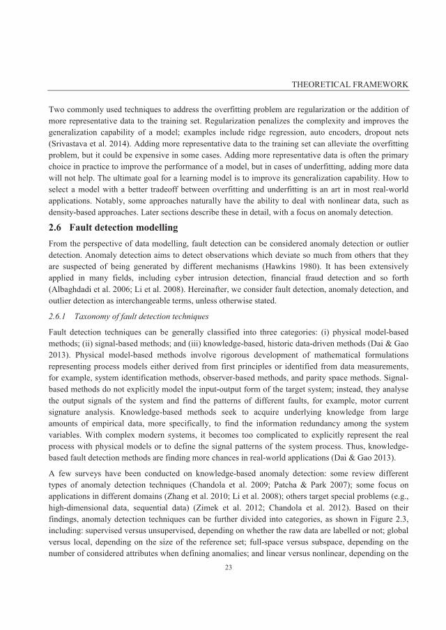
Fault detection techniques can be generally classified into three categories: (i) physical model-based methods; (ii) signal-based methods; and (iii) knowledge-based, historic data-driven methods (Dai & Gao 2013). Physical model-based methods involve rigorous development of mathematical formulations representing process models either derived from first principles or identified from data measurements, for example, system identification methods, observer-based methods, and parity space methods. Signal-based methods do not explicitly model the input-output form of the target system; instead, they analyse the output signals of the system and find the patterns of different faults, for example, motor current signature analysis. Knowledge-based methods seek to acquire underlying knowledge from large amounts of empirical data, more specifically, to find the information redundancy among the system variables. With complex modern systems, it becomes too complicated to explicitly represent the real process with physical models or to define the signal patterns of the system process. Thus, knowledge-based fault detection methods are finding more chances in real-world applications (Dai & Gao 2013).
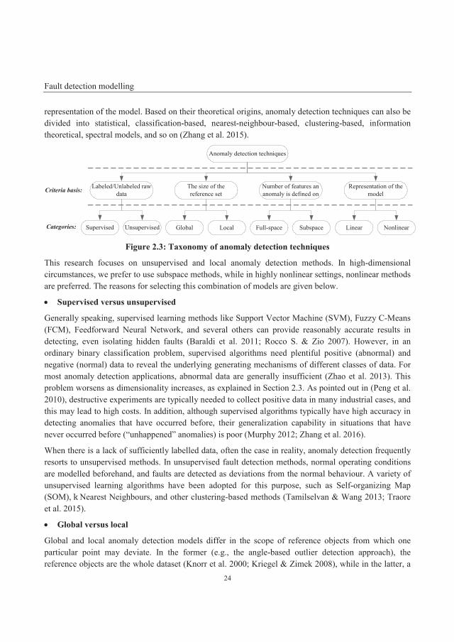
A few surveys have been conducted on knowledge-based anomaly detection: some review different types of anomaly detection techniques (Chandola et al. 2009; Patcha & Park 2007); some focus on applications in different domains (Zhang et al. 2010; Li et al. 2008); others target special problems (e.g., high-dimensional data, sequential data) (Zimek et al. 2012; Chandola et al. 2012). Based on their findings, anomaly detection techniques can be further divided into categories, as shown in Figure 2.3, including: supervised versus unsupervised, depending on whether the raw data are labelled or not; global versus local, depending on the size of the reference set; full-space versus subspace, depending on the number of considered attributes when defining anomalies; and linear versus nonlinear, depending on the
Fault detection modelling
24
representation of the model. Based on their theoretical origins, anomaly detection techniques can also be divided into statistical, classification-based, nearest-neighbour-based, clustering-based, information theoretical, spectral models, and so on (Zhang et al. 2015).
Figure 2.3: Taxonomy of anomaly detection techniques
This research focuses on unsupervised and local anomaly detection methods. In high-dimensional circumstances, we prefer to use subspace methods, while in highly nonlinear settings, nonlinear methods are preferred. The reasons for selecting this combination of models are given below.
Supervised versus unsupervised
Generally speaking, supervised learning methods like Support Vector Machine (SVM), Fuzzy C-Means (FCM), Feedforward Neural Network, and several others can provide reasonably accurate results in detecting, even isolating hidden faults (Baraldi et al. 2011; Rocco S. & Zio 2007). However, in an ordinary binary classification problem, supervised algorithms need plentiful positive (abnormal) and negative (normal) data to reveal the underlying generating mechanisms of different classes of data. For most anomaly detection applications, abnormal data are generally insufficient (Zhao et al. 2013). This problem worsens as dimensionality increases, as explained in Section 2.3. As pointed out in (Peng et al. 2010), destructive experiments are typically needed to collect positive data in many industrial cases, and this may lead to high costs. In addition, although supervised algorithms typically have high accuracy in detecting anomalies that have occurred before, their generalization capability in situations that have never occurred before (“unhappened” anomalies) is poor (Murphy 2012; Zhang et al. 2016).
When there is a lack of sufficiently labelled data, often the case in reality, anomaly detection frequently resorts to unsupervised methods. In unsupervised fault detection methods, normal operating conditions are modelled beforehand, and faults are detected as deviations from the normal behaviour. A variety of unsupervised learning algorithms have been adopted for this purpose, such as Self-organizing Map (SOM), k Nearest Neighbours, and other clustering-based methods (Tamilselvan & Wang 2013; Traore et al. 2015).
Global versus local
Global and local anomaly detection models differ in the scope of reference objects from which one particular point may deviate. In the former (e.g., the angle-based outlier detection approach), the reference objects are the whole dataset (Knorr et al. 2000; Kriegel & Zimek 2008), while in the latter, a
Criteria basis:
Categories:
Anomaly detection techniques
Number of features an anomaly is defined on
Supervised Unsupervised
The size of the reference set
Global Local Full-space Subspace
Labeled/Unlabeled raw data
Representation of the model
Linear Nonlinear

THEORETICAL FRAMEWORK
25
subset of all the data instances (e.g., nearest neighbours in the Local Outlier Factor approach) is taken into account (Breunig et al. 2000). To recognize their differences and highlight the importance of deriving a local outlier measure, we take the example shown in Figure 2.4 and apply the Kernel Density Estimate (KDE) for anomaly detection approach to the dataset. The approach assumes that low probability density implies the occurrence of a sample does not conform to an underlying data generating mechanism, hence indicating a possible anomaly. Specifically, KDE estimates the density of each point using a kernel function and sets a threshold on this univariate density to single out anomalies.
Figure 2.4: Parzen window estimator for anomaly detection; as a global measure of outlierness; it may fail to detect the outlying point in the data
In Figure 2.4, point (the red asterisk) is an anomaly adjacent to the dense cluster C1 (the blue points) and far away from the scattered cluster C2 (the black points). Suppose norm is chosen as the distance measure, and the uniform kernel with width d is adopted in the kernel density estimate. Non-strictly speaking, the density of point , ( ), can be intuitively interpreted as the number of points falling in the d -ball (the dashed circle). Given the magnitude of d in Figure 2.4, ( ) may be higher than the density of many points in cluster C2. A threshold set for the density estimate that is large enough to capture point may also lead to a high Type I error, i.e., false alarm rate, because the density estimate here is a global measure of outlierness. Thus, it lacks the power to discriminate the outlying point from those points in a less dense cluster, C2.
A formal definition of a local outlier measure is given in (Breunig et al. 2000); the paper also discusses the problems of evaluating the outlierness of a point from a global view. Based on the LOF approach and many of its variants, a recent study has pointed out that the importance of defining the outlierness measure in a local sense is that a local outlierness measure is relatively more invariant to the fluctuations in the density estimate and, hence, is more comparable over a dataset with varying densities (Schubert et al. 2014). Many real-world datasets have a complex structure, and data are generated by various

Fault detection modelling
26
mechanisms. Under such circumstances, local outlier detection techniques are usually preferred over global ones in terms of accuracy (Kriegel & Zimek 2008).
Full-space versus subspace
Figure 2.5: Irrelevant attributes x and y conceal the deviation in relevant dimension z
In high-dimensional spaces, the degree of deviation in some attributes may be obscured or covered by other irrelevant attributes (Domingos 2012; Zimek et al. 2012; Houle et al. 2010). To explain this, we offer the following example. In Figure 2.5 (a), randomly generated samples are plotted in a three-dimensional coordinate system. An outlier is placed in the dataset and marked as a red cross. The outlier behaves normally in axes and , as indicated in Figure 2.5 (b), but deviates significantly from other points in the axis, as shown in Figure 2.5 (c). From the perspective of distance, the fact that the outlier lies close to the cluster centre in the and dimensions compensates for the deviation of the outlier from the centre of the dimension. From the perspective of probability, the high likelihood of the occurrence of the outlier in the and dimensions counteracts the low probability of an abnormal occurrence in the axis to some extent. Consequently, neither distance-based approaches nor statistical models can effectively detect the severity of abnormality in the relevant subspace, namely the dimension in this example. This effect of sunken abnormality becomes more severe as the number of irrelevant dimensions increases. As identified in (Zimek et al. 2012; Houle et al. 2010), when the ratio of relevant and irrelevant attributes is high, traditional outlier detection techniques can still work even in a very high-dimensional setting. However, a low ratio of relevant and irrelevant attributes may greatly impede the separability of different data-generating mechanisms, leading to deterioration in the accuracy of traditional anomaly detection techniques implemented in full-dimensional spaces. In light of this consideration, researchers have started to probe the use of subspace anomaly detection techniques (see Subsection 2.6.2).
Linear versus nonlinear
The power of linear methods to represent complex relationships between features is limited. When there are strong linear correlations among different features, linear methods may work well. At the expense of
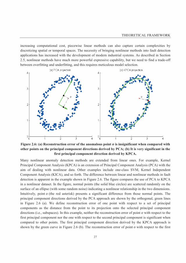
THEORETICAL FRAMEWORK
27
increasing computational cost, piecewise linear methods can also capture certain complexities by discretizing spatial or temporal spaces. The necessity of bringing nonlinear methods into fault detection applications has increased with the development of modern industrial systems. As described in Section 2.5, nonlinear methods have much more powerful expressive capability, but we need to find a trade-off between overfitting and underfitting, and this requires meticulous model selection.
Figure 2.6: (a) Reconstruction error of the anomalous point is insignificant when compared with other points on the principal component directions derived by PCA; (b) It is very significant in the
first principal component direction derived by KPCA.
Many nonlinear anomaly detection methods are extended from linear ones. For example, Kernel Principal Component Analysis (KPCA) is an extension of Principal Component Analysis (PCA) with the aim of dealing with nonlinear data. Other examples include one-class SVM, Kernel Independent Component Analysis (KICA), and so forth. The difference between linear and nonlinear methods in fault detection is apparent in the example shown in Figure 2.6. The figure compares the use of PCA to KPCA in a nonlinear dataset. In the figure, normal points (the solid blue circles) are scattered randomly on the surface of an ellipse (with some random noise) indicating a nonlinear relationship in the two dimensions. Intuitively, point (the red asterisk) presents a significant difference from those normal points. The principal component directions derived by the PCA approach are shown by the orthogonal, green lines in Figure 2.6 (a). We define reconstruction error of one point with respect to a set of principal components as the distance from the point to its projection onto the selected principal component directions (i.e., subspaces). In this example, neither the reconstruction error of point with respect to the first principal component nor the one with respect to the second principal component is significant when compared to other points. The first principal component direction derived by the KPCA approach is shown by the green curve in Figure 2.6 (b). The reconstruction error of point with respect to the first
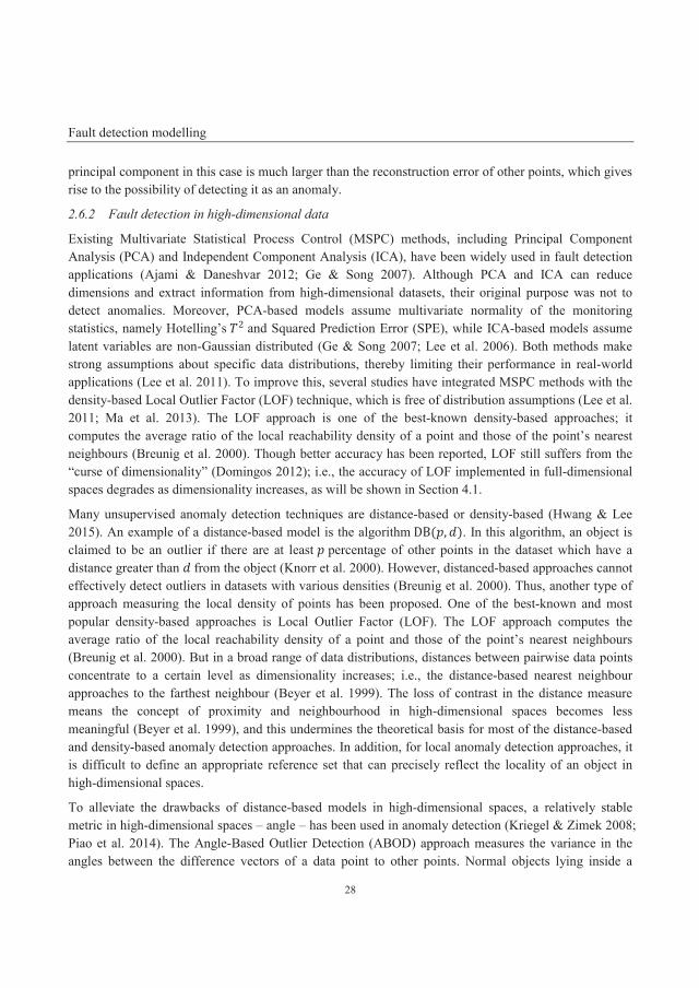
Fault detection modelling
28
principal component in this case is much larger than the reconstruction error of other points, which gives rise to the possibility of detecting it as an anomaly.
2.6.2 Fault detection in high-dimensional data
Existing Multivariate Statistical Process Control (MSPC) methods, including Principal Component Analysis (PCA) and Independent Component Analysis (ICA), have been widely used in fault detection applications (Ajami & Daneshvar 2012; Ge & Song 2007). Although PCA and ICA can reduce dimensions and extract information from high-dimensional datasets, their original purpose was not to detect anomalies. Moreover, PCA-based models assume multivariate normality of the monitoring statistics, namely Hotelling’s 2 and Squared Prediction Error (SPE), while ICA-based models assume latent variables are non-Gaussian distributed (Ge & Song 2007; Lee et al. 2006). Both methods make strong assumptions about specific data distributions, thereby limiting their performance in real-world applications (Lee et al. 2011). To improve this, several studies have integrated MSPC methods with the density-based Local Outlier Factor (LOF) technique, which is free of distribution assumptions (Lee et al. 2011; Ma et al. 2013). The LOF approach is one of the best-known density-based approaches; it computes the average ratio of the local reachability density of a point and those of the point’s nearest neighbours (Breunig et al. 2000). Though better accuracy has been reported, LOF still suffers from the “curse of dimensionality” (Domingos 2012); i.e., the accuracy of LOF implemented in full-dimensional spaces degrades as dimensionality increases, as will be shown in Section 4.1.
Many unsupervised anomaly detection techniques are distance-based or density-based (Hwang & Lee 2015). An example of a distance-based model is the algorithm DB( , ). In this algorithm, an object is claimed to be an outlier if there are at least percentage of other points in the dataset which have a distance greater than from the object (Knorr et al. 2000). However, distanced-based approaches cannot effectively detect outliers in datasets with various densities (Breunig et al. 2000). Thus, another type of approach measuring the local density of points has been proposed. One of the best-known and most popular density-based approaches is Local Outlier Factor (LOF). The LOF approach computes the average ratio of the local reachability density of a point and those of the point’s nearest neighbours (Breunig et al. 2000). But in a broad range of data distributions, distances between pairwise data points concentrate to a certain level as dimensionality increases; i.e., the distance-based nearest neighbour approaches to the farthest neighbour (Beyer et al. 1999). The loss of contrast in the distance measure means the concept of proximity and neighbourhood in high-dimensional spaces becomes less meaningful (Beyer et al. 1999), and this undermines the theoretical basis for most of the distance-based and density-based anomaly detection approaches. In addition, for local anomaly detection approaches, it is difficult to define an appropriate reference set that can precisely reflect the locality of an object in high-dimensional spaces.
To alleviate the drawbacks of distance-based models in high-dimensional spaces, a relatively stable metric in high-dimensional spaces – angle – has been used in anomaly detection (Kriegel & Zimek 2008; Piao et al. 2014). The Angle-Based Outlier Detection (ABOD) approach measures the variance in the angles between the difference vectors of a data point to other points. Normal objects lying inside a
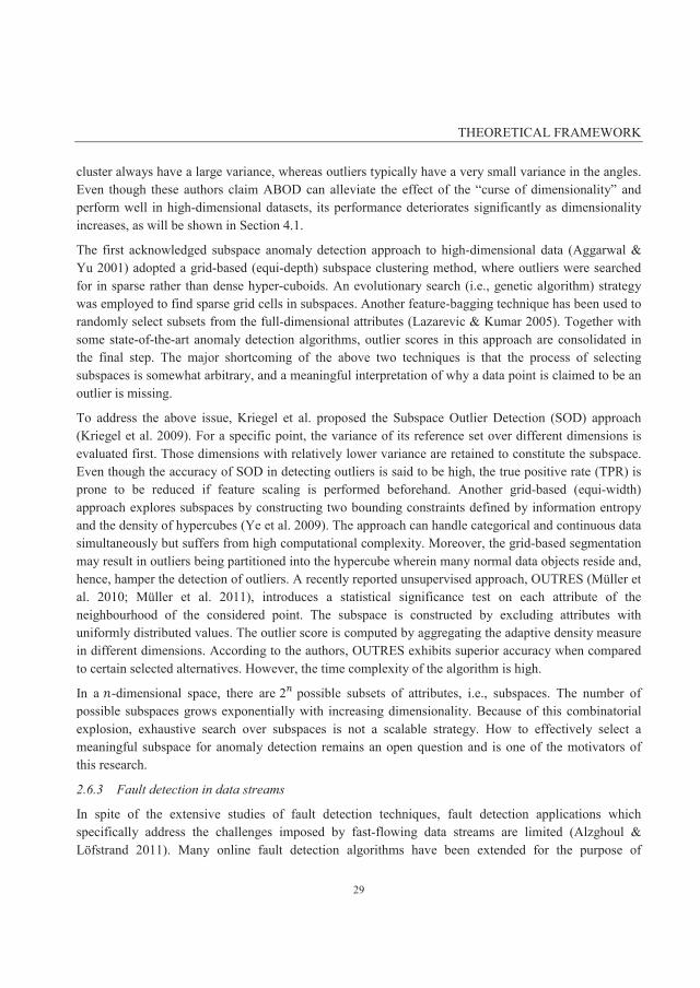
THEORETICAL FRAMEWORK
29
cluster always have a large variance, whereas outliers typically have a very small variance in the angles. Even though these authors claim ABOD can alleviate the effect of the “curse of dimensionality” and perform well in high-dimensional datasets, its performance deteriorates significantly as dimensionality increases, as will be shown in Section 4.1.
The first acknowledged subspace anomaly detection approach to high-dimensional data (Aggarwal & Yu 2001) adopted a grid-based (equi-depth) subspace clustering method, where outliers were searched for in sparse rather than dense hyper-cuboids. An evolutionary search (i.e., genetic algorithm) strategy was employed to find sparse grid cells in subspaces. Another feature-bagging technique has been used to randomly select subsets from the full-dimensional attributes (Lazarevic & Kumar 2005). Together with some state-of-the-art anomaly detection algorithms, outlier scores in this approach are consolidated in the final step. The major shortcoming of the above two techniques is that the process of selecting subspaces is somewhat arbitrary, and a meaningful interpretation of why a data point is claimed to be an outlier is missing.
To address the above issue, Kriegel et al. proposed the Subspace Outlier Detection (SOD) approach (Kriegel et al. 2009). For a specific point, the variance of its reference set over different dimensions is evaluated first. Those dimensions with relatively lower variance are retained to constitute the subspace. Even though the accuracy of SOD in detecting outliers is said to be high, the true positive rate (TPR) is prone to be reduced if feature scaling is performed beforehand. Another grid-based (equi-width) approach explores subspaces by constructing two bounding constraints defined by information entropy and the density of hypercubes (Ye et al. 2009). The approach can handle categorical and continuous data simultaneously but suffers from high computational complexity. Moreover, the grid-based segmentation may result in outliers being partitioned into the hypercube wherein many normal data objects reside and, hence, hamper the detection of outliers. A recently reported unsupervised approach, OUTRES (Müller et al. 2010; Müller et al. 2011), introduces a statistical significance test on each attribute of the neighbourhood of the considered point. The subspace is constructed by excluding attributes with uniformly distributed values. The outlier score is computed by aggregating the adaptive density measure in different dimensions. According to the authors, OUTRES exhibits superior accuracy when compared to certain selected alternatives. However, the time complexity of the algorithm is high.
In a -dimensional space, there are 2 possible subsets of attributes, i.e., subspaces. The number of possible subspaces grows exponentially with increasing dimensionality. Because of this combinatorial explosion, exhaustive search over subspaces is not a scalable strategy. How to effectively select a meaningful subspace for anomaly detection remains an open question and is one of the motivators of this research.
2.6.3 Fault detection in data streams
In spite of the extensive studies of fault detection techniques, fault detection applications which specifically address the challenges imposed by fast-flowing data streams are limited (Alzghoul & Löfstrand 2011). Many online fault detection algorithms have been extended for the purpose of
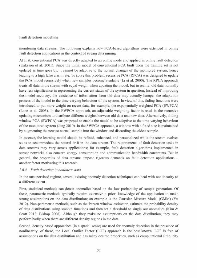
Fault detection modelling
30
monitoring data streams. The following explains how PCA-based algorithms were extended in online fault detection applications in the context of stream data mining.
At first, conventional PCA was directly adapted to an online mode and applied in online fault detection (Eriksson et al. 2001). Since the initial model of conventional PCA built upon the training set is not updated as time goes by, it cannot be adaptive to the normal changes of the monitored system, hence leading to a high false alarm rate. To solve this problem, recursive PCA (RPCA) was designed to update the PCA model recursively when new samples become available (Li et al. 2000). The RPCA approach treats all data in the stream with equal weight when updating the model, but in reality, old data normally have less significance in representing the current status of the system in question. Instead of improving the model accuracy, the existence of information from old data may actually hamper the adaptation process of the model to the time-varying behaviour of the system. In view of this, fading functions were introduced to put more weight on recent data, for example, the exponentially weighted PCA (EWPCA) (Lane et al. 2003). In the EWPCA approach, an adjustable weighting factor is used in the recursive updating mechanism to distribute different weights between old data and new data. Alternatively, sliding window PCA (SWPCA) was proposed to enable the model to be adaptive to the time-varying behaviour of the monitored system (Jeng 2010). In the SWPCA approach, a window with a fixed size is maintained by augmenting the newest normal sample into the window and discarding the oldest sample.
In essence, the learning model should be refined, enhanced, and personalized while the stream evolves so as to accommodate the natural drift in the data stream. The requirements of fault detection tasks in data streams may vary across applications; for example, fault detection algorithms implemented in sensor networks also concern energy consumption and communication bandwidth constraints. But in general, the properties of data streams impose rigorous demands on fault detection applications – another factor motivating this research.
2.6.4 Fault detection in nonlinear data
In the unsupervised regime, several existing anomaly detection techniques can deal with nonlinearity to a different extent.
First, statistical methods can detect anomalies based on the low probability of sample generation. Of these, parametric methods typically require extensive a priori knowledge of the application to make strong assumptions on the data distribution; an example is the Gaussian Mixture Model (GMM) (Yu 2012). Non-parametric methods, such as the Parzen window estimator, estimate the probability density of data distributions using smooth functions and then set a threshold to single out anomalies (Kim & Scott 2012; Bishop 2006). Although they make no assumptions on the data distribution, they may perform badly when there are different density regions in the data.
Second, density-based approaches (in a spatial sense) are used for anomaly detection in the presence of nonlinearity; of these, the Local Outlier Factor (LOF) approach is the best known. LOF is free of assumptions on the data distribution and has many desired properties, such as computational simplicity
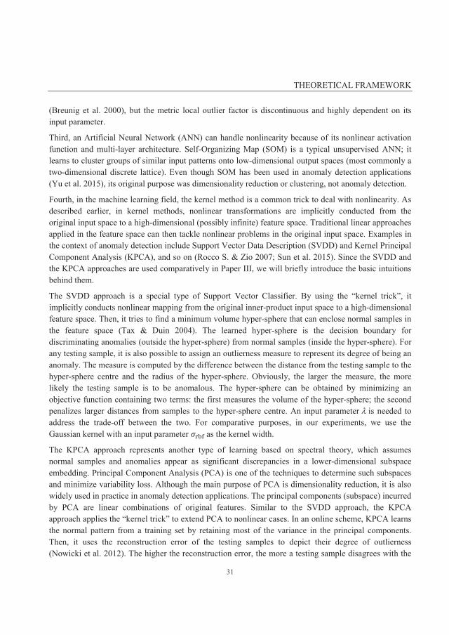
THEORETICAL FRAMEWORK
31
(Breunig et al. 2000), but the metric local outlier factor is discontinuous and highly dependent on its input parameter.
Third, an Artificial Neural Network (ANN) can handle nonlinearity because of its nonlinear activation function and multi-layer architecture. Self-Organizing Map (SOM) is a typical unsupervised ANN; it learns to cluster groups of similar input patterns onto low-dimensional output spaces (most commonly a two-dimensional discrete lattice). Even though SOM has been used in anomaly detection applications (Yu et al. 2015), its original purpose was dimensionality reduction or clustering, not anomaly detection.
Fourth, in the machine learning field, the kernel method is a common trick to deal with nonlinearity. As described earlier, in kernel methods, nonlinear transformations are implicitly conducted from the original input space to a high-dimensional (possibly infinite) feature space. Traditional linear approaches applied in the feature space can then tackle nonlinear problems in the original input space. Examples in the context of anomaly detection include Support Vector Data Description (SVDD) and Kernel Principal Component Analysis (KPCA), and so on (Rocco S. & Zio 2007; Sun et al. 2015). Since the SVDD and the KPCA approaches are used comparatively in Paper III, we will briefly introduce the basic intuitions behind them.
The SVDD approach is a special type of Support Vector Classifier. By using the “kernel trick”, it implicitly conducts nonlinear mapping from the original inner-product input space to a high-dimensional feature space. Then, it tries to find a minimum volume hyper-sphere that can enclose normal samples in the feature space (Tax & Duin 2004). The learned hyper-sphere is the decision boundary for discriminating anomalies (outside the hyper-sphere) from normal samples (inside the hyper-sphere). For any testing sample, it is also possible to assign an outlierness measure to represent its degree of being an anomaly. The measure is computed by the difference between the distance from the testing sample to the hyper-sphere centre and the radius of the hyper-sphere. Obviously, the larger the measure, the more likely the testing sample is to be anomalous. The hyper-sphere can be obtained by minimizing an objective function containing two terms: the first measures the volume of the hyper-sphere; the second penalizes larger distances from samples to the hyper-sphere centre. An input parameter is needed to address the trade-off between the two. For comparative purposes, in our experiments, we use the Gaussian kernel with an input parameter as the kernel width.
The KPCA approach represents another type of learning based on spectral theory, which assumes normal samples and anomalies appear as significant discrepancies in a lower-dimensional subspace embedding. Principal Component Analysis (PCA) is one of the techniques to determine such subspaces and minimize variability loss. Although the main purpose of PCA is dimensionality reduction, it is also widely used in practice in anomaly detection applications. The principal components (subspace) incurred by PCA are linear combinations of original features. Similar to the SVDD approach, the KPCA approach applies the “kernel trick” to extend PCA to nonlinear cases. In an online scheme, KPCA learns the normal pattern from a training set by retaining most of the variance in the principal components. Then, it uses the reconstruction error of the testing samples to depict their degree of outlierness (Nowicki et al. 2012). The higher the reconstruction error, the more a testing sample disagrees with the
Summary of framework
32
learned pattern and the more likely it is to be an anomaly. Again, in the experiments, we use the Gaussian kernel with width parameter . Further, we let denote the proportion of variance retained in subspace.
The main problem with the kernel methods is a lack of interpretability and the difficulty of tuning input parameters in an unsupervised fashion. Since the nonlinear transformations are conducted implicitly, the function mapping the samples from the original space to the new feature space is totally intractable, leading to a lack of interpretability. Moreover, it is difficult to tune hyper-parameters in these methods. An inappropriate setting of input parameters may easily lead to underfitting or overfitting, and unfortunately, there are no general rules on how to tune these parameters in an unsupervised setting.
To the best of our knowledge, none of the above introduced anomaly detection approaches has all the desired properties, i.e., smoothness, effectiveness, robustness, and interpretability, in their measure of local outlierness. This leads to the final motivation of the research: the need to find a better approach to detecting anomalies for nonlinear systems.
2.7 Summary of framework Big Data with immense value are often buried but can be excavated to support decision-making. Big Data can be characterized by the three “Vs”, volume, velocity and variety, and by “c”, complexity. eMaintenance data have these characteristics, thus motivating the development and adoption of Big Data analytics.
Fault detection is one of the means to approach eMaintenance with the aim of transforming maintenance practices from reactive to proactive. From a data modelling point of view, high dimensionality, fast-flowing data streams, and nonlinearity are major challenges in fault detection applications. High dimensionality may cause the notorious “curse of dimensionality” and lead to deterioration in the accuracy of fault detection algorithms. Fast-flowing data streams require fault detection algorithms with low computing complexity and able to give real-time or near real-time responses upon the arrival of new samples. Nonlinearity requires fault detection models to have sufficiently expressive power and to avoid underfitting or overfitting problems. All these challenges need to be addressed cautiously in Big Data analytics.
Most of the existing fault detection techniques work on relatively low-dimensional spaces. Even though some can perform dimension reduction, such as PCA and ICA, they were not designed for the purpose of fault detection. Furthermore, both PCA and ICA have strong assumptions on the distribution of the measurements, thereby limiting their performance in real-world applications. Theoretical studies on high-dimensional fault detection mainly focus on detecting abnormalities on subspace projections of the original space, but these methods are either arbitrary in selecting subspaces or computationally intensive. An efficient way of selecting meaningful subspaces needs to be developed.
In response to the requirements of fast-flowing data streams, advances have been made in the development of data stream processing tools and in data modelling. With respect to the latter, several strategies have been proposed to adapt existing models to an online mode so they can be applicable in

THEORETICAL FRAMEWORK
33
stream data mining, e.g., the sliding window strategy. The key to these methods is that the learning model should be refined, enhanced, and personalized while the stream evolves so as to accommodate the natural drift in the data stream. High-dimensional data streams are becoming ubiquitous in industrial systems, but few fault detection-related studies have simultaneously tackled the challenges associated with high dimensionality and data streams. Big Data analytics need to be further developed to cope with these challenges.
Existing nonlinear fault detection approaches cannot provide satisfactory performance in terms of smoothness, effectiveness, robustness and interpretability. The Parzen window estimate approach provides a global measure of outlierness which may fail to detect anomalies from datasets with various densities. The accuracy of the LOF approach is highly dependent on its input parameters, and its measure of outlierness is discontinuous. The kernel methods lack interpretability, and no general rules can be applied to the model selection procedure, which may lead to underfitting or overfitting problems. New approaches are needed to address all these problems.

34
35
CHAPTER 3. RESEARCH METHODOLOGY This chapter presents some theories of research methodology and explains the choices made for this research.
3.1 Research design Research is an original contribution to the existing stock of knowledge, thus allowing its advancement (Kothari 2011). Technically, it has been defined as a “systematic method consisting of enunciating the problem, formulating a hypothesis, collecting the facts or data, analysing the facts and reaching certain conclusions either in the form of solutions towards the concerned problem or in certain generalizations for some theoretical formulation” (Kothari 2011). Research approaches can be broadly divided into quantitative, qualitative, and mixed methods. Quantitative research is based on the measurement of quantity or amount; qualitative research is based on non-numerical data; mixed methods fall somewhere between the other two. A detailed explanation of these approaches appears in (Creswell 2013). Further, depending on the research purpose, research can be subdivided into exploratory research, descriptive research and explanatory research.
Exploratory research is the initial study to explore a phenomenon or to achieve new insights into it. It attempts to gain familiarity with the phenomenon and lay the groundwork for future studies. Exploratory research often adopts qualitative approaches; it might involve a literature study, focus group interviews or other methods. The exploration of new phenomena through these methods may deepen the researchers’ understanding, indicate new research directions, or facilitate the selection of methods to be used in a subsequent study.
Descriptive research seeks to accurately portray the characteristics of a phenomenon. It can take a qualitative, quantitative or a mixed approach. It often involves gathering data describing events; it then organizes, tabulates, depicts and describes the collected data. Observational methods, surveys and case studies are frequently used in descriptive research. Descriptive research can produce useful insights and lead to the formation of a hypothesis.
Explanatory research, also known as causal research, aims to test the hypothesis of a cause and effect relationship between variables to explain the nature of a certain phenomenon. Normally, quantitative approaches are applied in explanatory research. Statistical techniques, especially hypothesis testing, provide a way to disclose the causal relationships within a phenomenon. Explanatory research may
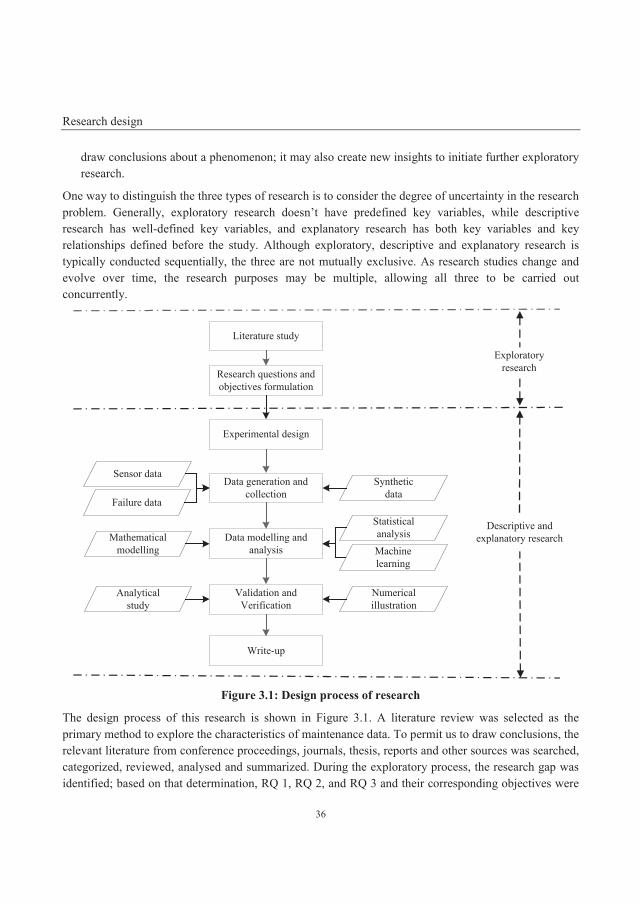
Research design
36
draw conclusions about a phenomenon; it may also create new insights to initiate further exploratory research.
One way to distinguish the three types of research is to consider the degree of uncertainty in the research problem. Generally, exploratory research doesn’t have predefined key variables, while descriptive research has well-defined key variables, and explanatory research has both key variables and key relationships defined before the study. Although exploratory, descriptive and explanatory research is typically conducted sequentially, the three are not mutually exclusive. As research studies change and evolve over time, the research purposes may be multiple, allowing all three to be carried out concurrently.
Figure 3.1: Design process of research
The design process of this research is shown in Figure 3.1. A literature review was selected as the primary method to explore the characteristics of maintenance data. To permit us to draw conclusions, the relevant literature from conference proceedings, journals, thesis, reports and other sources was searched, categorized, reviewed, analysed and summarized. During the exploratory process, the research gap was identified; based on that determination, RQ 1, RQ 2, and RQ 3 and their corresponding objectives were
Literature study
Research questions and objectives formulation
Experimental design
Data generation and collection
Data modelling and analysis
Validation and Verification
Write-up
Exploratory research
Descriptive and explanatory research
Synthetic data
Mathematical modelling
Statistical analysisMachine learning
Sensor data
Failure data
Analytical study
Numerical illustration
RESEARCH METHODOLOGY
37
formulated. Since the major difference between RQ 1, RQ 2, and RQ 3 is the nature of the input data, each basically follows the same research process. In the following, we explain the lower part of Figure 3.1 by mapping it to the process of answering RQ 1.
After framing RQ 1 and its objectives, we created an experimental design to define independent variables and dependent variables and to determine how to manipulate independent variables. In our case, the independent variables are fault-relevant variables (e.g., the first five dimensions in Figure 3.2) and the dependent variable is essentially the severity of potential faults (e.g., the local outlierness of faulty samples). Note the dependent variable is not measurable; instead, it is given as an output from the model. When the fault-relevant variables are manipulated, the local outlierness of the faulty samples changes accordingly, thus allowing their detection. This manipulation was done using synthetic data (see Subsection 3.2.1). The data modelling and analysis constitute the major contribution of the research. The modelling combines several techniques from different disciplines, including machine learning, statistical analysis and mathematical modelling, to compute the local outlierness of a sample and determine whether the sample is faulty or not. Analytical analysis was conducted to prove the theoretical merits of the proposed approach (e.g., the boundedness of the measure of the local outlier score), and numerical illustrations were applied to validate it. In a final step, the work was written up in the form of conference papers, journal papers and the present thesis.
We used both descriptive and explanatory research to answer the research question. In keeping with the definition of descriptive research, defining and calculating the local outlierness of a sample can be considered descriptive of the health state of the monitored system. Meanwhile, our preliminary explanations of potential faults through the use of feature ordering in the retained subspaces are explanatory. This latter research can be extended to probe the cause of faults (fault diagnosis) and to predict future failures (prognosis).
3.2 Data generation and collection 3.2.1 Synthetic data generation
In all three papers, synthetic data were generated and used for validation purposes. Generating synthetic data is a common practice in many research fields. Synthetic data are a feasible alternative to real-world data in a variety of situations when real-world data are difficult to obtain for reasons of time, cost, privacy or other concerns. These data are normally employed as a substitute for real-world data; they can provide a controllable testing environment that meets specific conditions. They are especially useful for the purposes of validation, simulation or preliminary proof of a concept.
Occasionally, although real-world data are available, specific needs or certain conditions for conducting a particular study may not be satisfied by real-world data. Under such circumstances, synthetic data can be used because their data generating mechanisms are controllable. For example, in Paper I, synthetic datasets are used because real-world data cannot fulfil the requirements to conduct a comprehensive study. The specific reasons for using synthetic datasets in Paper I are the following: first, to compare the suggested algorithm with alternatives and examine their performance under various dimensionality
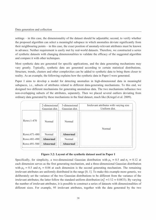
Data generation and collection
38
settings – in this case, the dimensionality of the dataset should be adjustable; second, to verify whether the proposed algorithm can select a meaningful subspace in which anomalies deviate significantly from their neighbouring points – in this case, the exact position of anomaly-relevant attributes must be known in advance. Neither requirement is easily met by real-world datasets. Therefore, we constructed a series of synthetic datasets with changing dimensionalities to validate the efficacy of the suggested algorithm and compare it with other techniques.
Most synthetic data are generated for specific applications, and the data generating mechanisms may vary greatly. Typically, synthetic data are generated according to certain statistical distributions. Structure, trends, clusters and other complexities can be added to synthetic data to bring them closer to reality. As an example, the following explains how the synthetic data in Paper I were generated.
Paper I aims to develop a model for detecting anomalies in high-dimensional data in meaningful subspaces, i.e., subsets of attributes related to different data-generating mechanisms. To this end, we designed two different mechanisms for generating anomalous data. The two mechanisms influence two non-overlapping subsets of the attributes, separately. Then we placed several outliers deviating from ordinary data generated by these mechanisms in the final dataset, much like (Kriegel et al. 2009).
Figure 3.2: Layout of the synthetic dataset used in Paper I
Specifically, for simplicity, a two-dimensional Gaussian distribution with = 0.5 and = 0.12 at each dimension serves as the first generating mechanism, and a three-dimensional Gaussian distribution with = 0.5 and = 0.04 at each dimension is the second generating mechanism. The remaining irrelevant attributes are uniformly distributed in the range [0, 1]. To make this example more generic, we deliberately set the variance of the two Gaussian distributions to be different from the variance of the irrelevant attributes; the latter follow the standard uniform distribution ( =1/12 0.0833). By varying the number of irrelevant attributes, it is possible to construct a series of datasets with dimensionalities of different sizes. For example, 95 irrelevant attributes, together with the data generated by the two
Rows:1-470
NormalRows:471-480
Rows:481-490
Rows:491-500
2-dimensionalGaussian dist.
3-dimensionalGaussian dist.
Irrelevant attributes with varying sizeUniform dist.
Normal Normal
Abnormal
Abnormal
AbnormalAbnormal
Normal
Normal
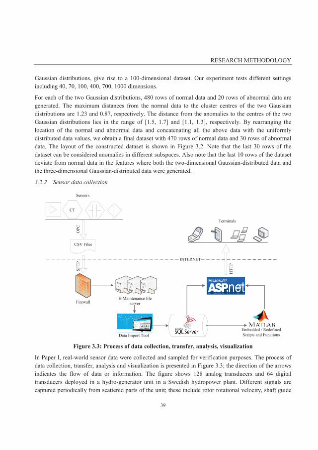
RESEARCH METHODOLOGY
39
Gaussian distributions, give rise to a 100-dimensional dataset. Our experiment tests different settings including 40, 70, 100, 400, 700, 1000 dimensions.
For each of the two Gaussian distributions, 480 rows of normal data and 20 rows of abnormal data are generated. The maximum distances from the normal data to the cluster centres of the two Gaussian distributions are 1.23 and 0.87, respectively. The distance from the anomalies to the centres of the two Gaussian distributions lies in the range of [1.5, 1.7] and [1.1, 1.3], respectively. By rearranging the location of the normal and abnormal data and concatenating all the above data with the uniformly distributed data values, we obtain a final dataset with 470 rows of normal data and 30 rows of abnormal data. The layout of the constructed dataset is shown in Figure 3.2. Note that the last 30 rows of the dataset can be considered anomalies in different subspaces. Also note that the last 10 rows of the dataset deviate from normal data in the features where both the two-dimensional Gaussian-distributed data and the three-dimensional Gaussian-distributed data were generated.
3.2.2 Sensor data collection
OPC
Sensors
CT
CSV Files
FirewallE-Maintenance file
server
SFTP
Data Import ToolEmbedded / Redefined Scripts and Functions
Terminals
INTERNET
HTT
P
Figure 3.3: Process of data collection, transfer, analysis, visualization
In Paper I, real-world sensor data were collected and sampled for verification purposes. The process of data collection, transfer, analysis and visualization is presented in Figure 3.3; the direction of the arrows indicates the flow of data or information. The figure shows 128 analog transducers and 64 digital transducers deployed in a hydro-generator unit in a Swedish hydropower plant. Different signals are captured periodically from scattered parts of the unit; these include rotor rotational velocity, shaft guide
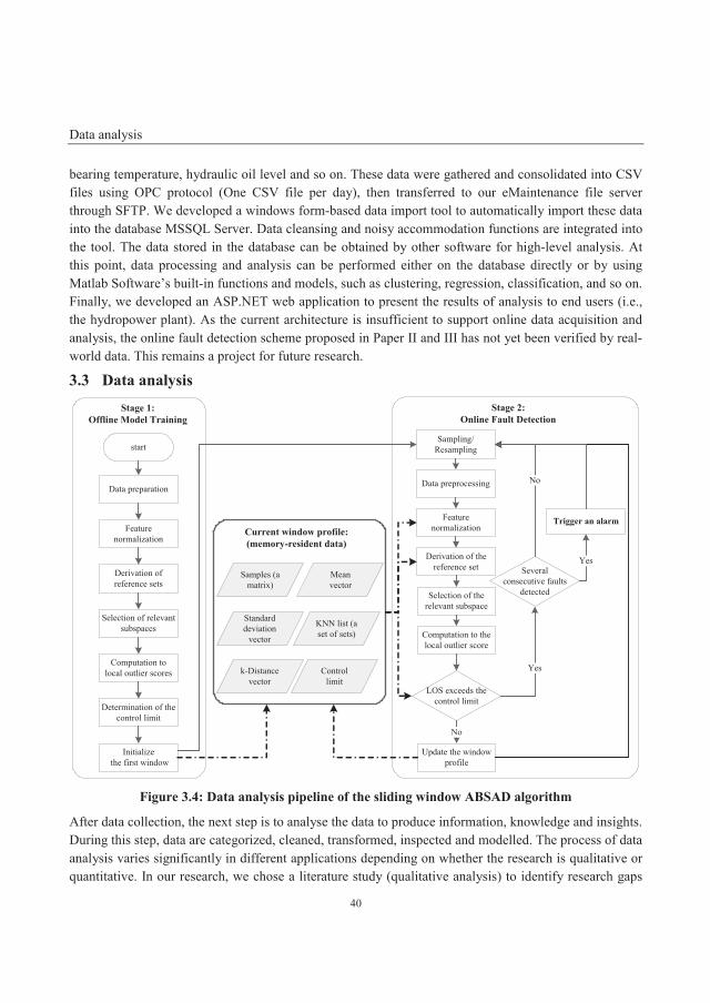
Data analysis
40
bearing temperature, hydraulic oil level and so on. These data were gathered and consolidated into CSV files using OPC protocol (One CSV file per day), then transferred to our eMaintenance file server through SFTP. We developed a windows form-based data import tool to automatically import these data into the database MSSQL Server. Data cleansing and noisy accommodation functions are integrated into the tool. The data stored in the database can be obtained by other software for high-level analysis. At this point, data processing and analysis can be performed either on the database directly or by using Matlab Software’s built-in functions and models, such as clustering, regression, classification, and so on. Finally, we developed an ASP.NET web application to present the results of analysis to end users (i.e., the hydropower plant). As the current architecture is insufficient to support online data acquisition and analysis, the online fault detection scheme proposed in Paper II and III has not yet been verified by real-world data. This remains a project for future research.
3.3 Data analysis
Figure 3.4: Data analysis pipeline of the sliding window ABSAD algorithm
After data collection, the next step is to analyse the data to produce information, knowledge and insights. During this step, data are categorized, cleaned, transformed, inspected and modelled. The process of data analysis varies significantly in different applications depending on whether the research is qualitative or quantitative. In our research, we chose a literature study (qualitative analysis) to identify research gaps
Stage 1:Offline Model Training
Stage 2:Online Fault Detection
Data preparation
Feature normalization
Derivation of reference sets
Selection of relevant subspaces
Computation to local outlier scores
Determination of the control limit
start
Data preprocessing
Feature normalization
Derivation of the reference set
Selection of the relevant subspace
Computation to the local outlier score
Current window profile:(memory-resident data)
LOS exceeds the control limit
Samples (a matrix)
Several consecutive faults
detected
Yes
Trigger an alarm
Yes
No
Mean vector
Standard deviation
vector
k-Distance vector
Control limit
No
Update the window profile
Sampling/Resampling
KNN list (a set of sets)
Initialize the first window
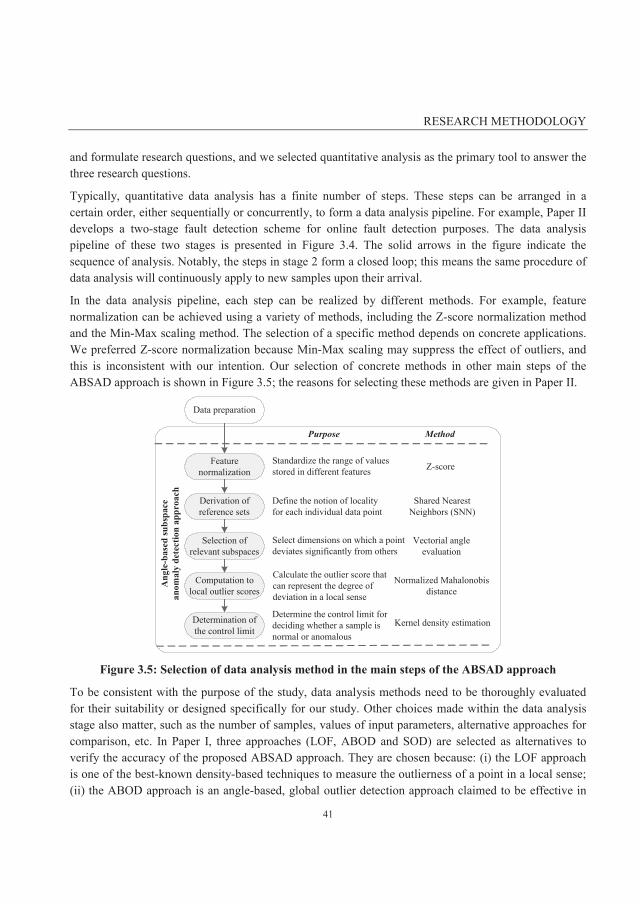
RESEARCH METHODOLOGY
41
and formulate research questions, and we selected quantitative analysis as the primary tool to answer the three research questions.
Typically, quantitative data analysis has a finite number of steps. These steps can be arranged in a certain order, either sequentially or concurrently, to form a data analysis pipeline. For example, Paper II develops a two-stage fault detection scheme for online fault detection purposes. The data analysis pipeline of these two stages is presented in Figure 3.4. The solid arrows in the figure indicate the sequence of analysis. Notably, the steps in stage 2 form a closed loop; this means the same procedure of data analysis will continuously apply to new samples upon their arrival.
In the data analysis pipeline, each step can be realized by different methods. For example, feature normalization can be achieved using a variety of methods, including the Z-score normalization method and the Min-Max scaling method. The selection of a specific method depends on concrete applications. We preferred Z-score normalization because Min-Max scaling may suppress the effect of outliers, and this is inconsistent with our intention. Our selection of concrete methods in other main steps of the ABSAD approach is shown in Figure 3.5; the reasons for selecting these methods are given in Paper II.
Figure 3.5: Selection of data analysis method in the main steps of the ABSAD approach
To be consistent with the purpose of the study, data analysis methods need to be thoroughly evaluated for their suitability or designed specifically for our study. Other choices made within the data analysis stage also matter, such as the number of samples, values of input parameters, alternative approaches for comparison, etc. In Paper I, three approaches (LOF, ABOD and SOD) are selected as alternatives to verify the accuracy of the proposed ABSAD approach. They are chosen because: (i) the LOF approach is one of the best-known density-based techniques to measure the outlierness of a point in a local sense; (ii) the ABOD approach is an angle-based, global outlier detection approach claimed to be effective in
Ang
le-b
ased
subs
pace
an
omal
y de
tect
ion
appr
oach
Define the notion of locality for each individual data point
Standardize the range of values stored in different features
Select dimensions on which a point deviates significantly from others
Calculate the outlier score that can represent the degree of deviation in a local sense
Purpose Method
Z-score
Shared Nearest Neighbors (SNN)
Vectorial angle evaluation
Normalized Mahalonobis distance
Data preparation
Determination of the control limit
Feature normalization
Derivation of reference sets
Selection of relevant subspaces
Computation to local outlier scores
Determine the control limit for deciding whether a sample is normal or anomalous
Kernel density estimation

Data analysis
42
high-dimensional spaces; (iii) the SOD approach is very similar to ours but it selects subspaces based on the variance of the reference points on different dimensions.
43
CHAPTER 4. RESULTS AND DISCUSSION This chapter gives the results and discussion corresponding to each research question.
4.1 Results and discussion related to RQ 1 The first research question was stated as: How can patterns be extracted from maintenance Big Data with high dimensionality characteristics?
To answer this question, we developed an Angle-based Subspace Anomaly Detection approach. The aim was to detect anomalies in high-dimensional datasets while maintaining the detection accuracy. The approach selects relevant subspaces from full-dimensional space based on the angle between all pairs of two lines for one specific anomaly candidate: the first line is connected by the concerned point and the centre of its surrounding points; the second line is one of the axis-parallel lines. The angle is calculated by the metric “pairwise cosine” ( ). The is the average absolute value of cosine between the projections of the two lines on all possible two-dimensional spaces. Each of these two-dimensional spaces is spanned by the axis dimension in question and one of the remaining dimensions of the feature space. The dimensions with a relatively large value are selected to constitute the targeted subspace. To compute the local outlierness of the anomaly candidate in its subspace projection, a normalized Mahalanobis distance measure is used. The proposed approach was evaluated using both synthetic data and a real-world dataset, and the results are reported separately below.
4.1.1 Validation using synthetic datasets
To validate the ABSAD algorithm, we constructed synthetic datasets with various dimensionality settings. We compared the proposed algorithm with several other prominent anomaly detection techniques, including LOF, ABOD, and SOD. We used the well-established Receiver Operating Characteristic (ROC) curve as the accuracy indicator to compare the algorithms in different datasets. The ROC curve is a graphical tool that can display the accuracy of a binary classifier. It plots the True Positive Rate (TPR) against the False Positive Rate (FPR) at various threshold settings; hence, it is threshold independent. The larger the area under the curve (AUC), the better accuracy a classifier can achieve.
The experiments indicate that the suggested ABSAD algorithm outperforms the other three in various high-dimensional settings. The comparison of the accuracy of the four algorithms in three different
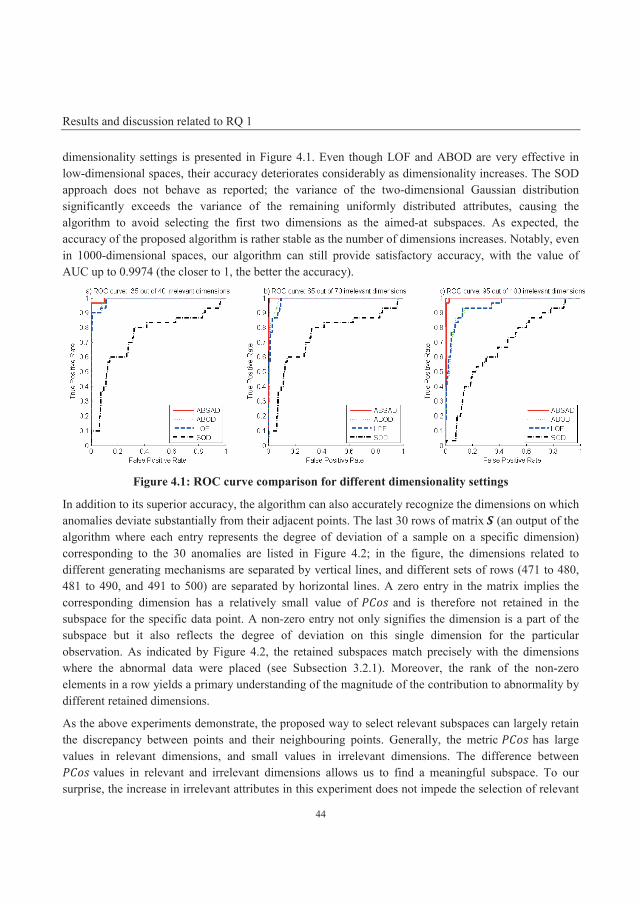
Results and discussion related to RQ 1
44
dimensionality settings is presented in Figure 4.1. Even though LOF and ABOD are very effective in low-dimensional spaces, their accuracy deteriorates considerably as dimensionality increases. The SOD approach does not behave as reported; the variance of the two-dimensional Gaussian distribution significantly exceeds the variance of the remaining uniformly distributed attributes, causing the algorithm to avoid selecting the first two dimensions as the aimed-at subspaces. As expected, the accuracy of the proposed algorithm is rather stable as the number of dimensions increases. Notably, even in 1000-dimensional spaces, our algorithm can still provide satisfactory accuracy, with the value of AUC up to 0.9974 (the closer to 1, the better the accuracy).
Figure 4.1: ROC curve comparison for different dimensionality settings
In addition to its superior accuracy, the algorithm can also accurately recognize the dimensions on which anomalies deviate substantially from their adjacent points. The last 30 rows of matrix (an output of the algorithm where each entry represents the degree of deviation of a sample on a specific dimension) corresponding to the 30 anomalies are listed in Figure 4.2; in the figure, the dimensions related to different generating mechanisms are separated by vertical lines, and different sets of rows (471 to 480, 481 to 490, and 491 to 500) are separated by horizontal lines. A zero entry in the matrix implies the corresponding dimension has a relatively small value of and is therefore not retained in the subspace for the specific data point. A non-zero entry not only signifies the dimension is a part of the subspace but it also reflects the degree of deviation on this single dimension for the particular observation. As indicated by Figure 4.2, the retained subspaces match precisely with the dimensions where the abnormal data were placed (see Subsection 3.2.1). Moreover, the rank of the non-zero elements in a row yields a primary understanding of the magnitude of the contribution to abnormality by different retained dimensions.
As the above experiments demonstrate, the proposed way to select relevant subspaces can largely retain the discrepancy between points and their neighbouring points. Generally, the metric has large values in relevant dimensions, and small values in irrelevant dimensions. The difference between values in relevant and irrelevant dimensions allows us to find a meaningful subspace. To our surprise, the increase in irrelevant attributes in this experiment does not impede the selection of relevant
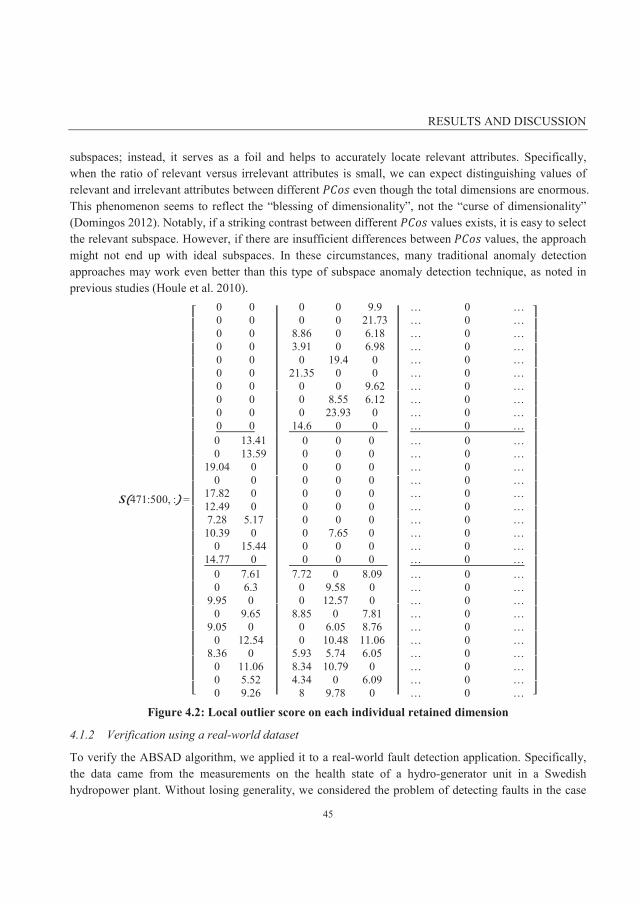
RESULTS AND DISCUSSION
45
subspaces; instead, it serves as a foil and helps to accurately locate relevant attributes. Specifically, when the ratio of relevant versus irrelevant attributes is small, we can expect distinguishing values of relevant and irrelevant attributes between different even though the total dimensions are enormous. This phenomenon seems to reflect the “blessing of dimensionality”, not the “curse of dimensionality” (Domingos 2012). Notably, if a striking contrast between different values exists, it is easy to select the relevant subspace. However, if there are insufficient differences between values, the approach might not end up with ideal subspaces. In these circumstances, many traditional anomaly detection approaches may work even better than this type of subspace anomaly detection technique, as noted in previous studies (Houle et al. 2010).
S((471:500, :) =
0 00 00 00 00 00 00 00 00 00 00 13.410 13.59
19.04 00 0
17.82 012.49 07.28 5.1710.39 0
0 15.4414.77 0
0 7.610 6.3
9.95 00 9.65
9.05 00 12.54
8.36 00 11.060 5.520 9.26
0 0 9.90 0 21.73
8.86 0 6.183.91 0 6.98
0 19.4 021.35 0 0
0 0 9.620 8.55 6.120 23.93 0
14.6 0 00 0 00 0 00 0 00 0 00 0 00 0 00 0 00 7.65 00 0 00 0 0
7.72 0 8.090 9.58 00 12.57 0
8.85 0 7.810 6.05 8.760 10.48 11.06
5.93 5.74 6.058.34 10.79 04.34 0 6.09
8 9.78 0
… 0 …… 0 …… 0 …… 0 …… 0 …… 0 …… 0 …… 0 …… 0 …… 0 …… 0 …… 0 …… 0 …… 0 …… 0 …… 0 …… 0 …… 0 …… 0 …… 0 …… 0 …… 0 …… 0 …… 0 …… 0 …… 0 …… 0 …… 0 …… 0 …… 0 …
Figure 4.2: Local outlier score on each individual retained dimension
4.1.2 Verification using a real-world dataset
To verify the ABSAD algorithm, we applied it to a real-world fault detection application. Specifically, the data came from the measurements on the health state of a hydro-generator unit in a Swedish hydropower plant. Without losing generality, we considered the problem of detecting faults in the case
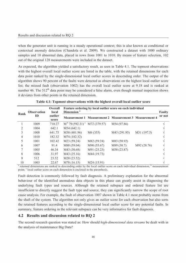
Results and discussion related to RQ 2
46
when the generator unit is running in a steady operational context; this is also known as conditional or contextual anomaly detection (Chandola et al. 2009). We constructed a dataset with 1000 ordinary samples and 10 abnormal data, placed in rows from 1001 to 1010. By means of feature selection, 102 out of the original 128 measurements were included in the dataset.
As expected, the algorithm yielded a satisfactory result, as seen in Table 4.1. The topmost observations with the highest overall local outlier score are listed in the table, with the retained dimensions for each data point ranked by the single-dimensional local outlier scores in descending order. The output of the algorithm shows 90 percent of the faults were detected as observations on the highest local outlier score list; the missed fault (observation 1002) has the overall local outlier score at 9.18 and is ranked at number 46. The 512th data point may be considered a false alarm, even though manual inspection shows it deviates from other points in the retained dimension.
Table 4.1: Topmost observations with the highest overall local outlier score
Rank Observation ID
Overall local
outlier score
Feature ordering by local outlier score on each individual Dimension a Faulty
or not Measurement 1 Measurement 2 Measurement 3 Measurement 4
1 1009 710.27 M b 79 (592.31) c M72 (379.57) M54 (97.86) 2 1004 642.1 M54 (642.1) 3 1008 641.75 M30 (401.96) M6 (355) M43 (291.95) M31 (197.5) 4 1010 182.32 M74 (182.32) 5 1001 102.42 M23 (59.24) M82 (59.24) M83 (58.92) 6 1007 91.4 M88 (59.04) M90 (55.67) M89 (30.7) M92 (28.76) 7 1005 46.34 M43 (30.68) M91 (25.23) M58 (23.87) 8 1006 31.97 M43 (25.16) M44 (19.73) 9 512 23.52 M20 (23.52) × 10 1003 22.67 M78 (16.15) M24 (15.91)
a retained dimensions are ranked in descending order by the local outlier score on each individual dimension; b measurement point; c local outlier score on each dimension is enclosed in the parenthesis.
Fault detection is commonly followed by fault diagnosis. A preliminary explanation for the abnormal behaviour of the identified anomalous data objects in this phase can greatly assist in diagnosing the underlying fault types and sources. Although the retained subspace and ordered feature list are insufficient to directly suggest the fault type and source, they can significantly narrow the scope of root cause analysis. For example, the fault of observation 1007 shown in Table 4.1 most probably stems from the shaft of the system. The algorithm not only gives an outlier score for each observation but also sorts the retained features according to the single-dimensional local outlier score for any potential faults. In summary, feature ordering in the relevant subspace can be very informative for fault diagnosis.
4.2 Results and discussion related to RQ 2 The second research question was stated as: How should high-dimensional data streams be dealt with in the analysis of maintenance Big Data?
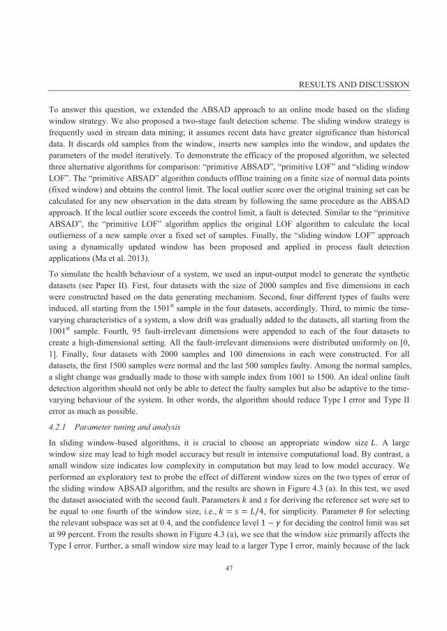
RESULTS AND DISCUSSION
47
To answer this question, we extended the ABSAD approach to an online mode based on the sliding window strategy. We also proposed a two-stage fault detection scheme. The sliding window strategy is frequently used in stream data mining; it assumes recent data have greater significance than historical data. It discards old samples from the window, inserts new samples into the window, and updates the parameters of the model iteratively. To demonstrate the efficacy of the proposed algorithm, we selected three alternative algorithms for comparison: “primitive ABSAD”, “primitive LOF” and “sliding window LOF”. The “primitive ABSAD” algorithm conducts offline training on a finite size of normal data points (fixed window) and obtains the control limit. The local outlier score over the original training set can be calculated for any new observation in the data stream by following the same procedure as the ABSAD approach. If the local outlier score exceeds the control limit, a fault is detected. Similar to the “primitive ABSAD”, the “primitive LOF” algorithm applies the original LOF algorithm to calculate the local outlierness of a new sample over a fixed set of samples. Finally, the “sliding window LOF” approach using a dynamically updated window has been proposed and applied in process fault detection applications (Ma et al. 2013).
To simulate the health behaviour of a system, we used an input-output model to generate the synthetic datasets (see Paper II). First, four datasets with the size of 2000 samples and five dimensions in each were constructed based on the data generating mechanism. Second, four different types of faults were induced, all starting from the 1501st sample in the four datasets, accordingly. Third, to mimic the time-varying characteristics of a system, a slow drift was gradually added to the datasets, all starting from the 1001st sample. Fourth, 95 fault-irrelevant dimensions were appended to each of the four datasets to create a high-dimensional setting. All the fault-irrelevant dimensions were distributed uniformly on [0, 1]. Finally, four datasets with 2000 samples and 100 dimensions in each were constructed. For all datasets, the first 1500 samples were normal and the last 500 samples faulty. Among the normal samples, a slight change was gradually made to those with sample index from 1001 to 1500. An ideal online fault detection algorithm should not only be able to detect the faulty samples but also be adaptive to the time-varying behaviour of the system. In other words, the algorithm should reduce Type I error and Type II error as much as possible.
4.2.1 Parameter tuning and analysis
In sliding window-based algorithms, it is crucial to choose an appropriate window size . A large window size may lead to high model accuracy but result in intensive computational load. By contrast, a small window size indicates low complexity in computation but may lead to low model accuracy. We performed an exploratory test to probe the effect of different window sizes on the two types of error of the sliding window ABSAD algorithm, and the results are shown in Figure 4.3 (a). In this test, we used the dataset associated with the second fault. Parameters and for deriving the reference set were set to be equal to one fourth of the window size, i.e., = = /4, for simplicity. Parameter for selecting the relevant subspace was set at 0.4, and the confidence level 1 for deciding the control limit was set at 99 percent. From the results shown in Figure 4.3 (a), we see that the window size primarily affects the Type I error. Further, a small window size may lead to a larger Type I error, mainly because of the lack

Results and discussion related to RQ 2
48
of representative neighbouring points in the window to support the normality of a normal sample. Meanwhile, the Type I error tends to increase slightly as the window size goes above 900; this may be caused by the inadequacy of the model to adapt to the time-varying characteristics of the system. Thus, an ideal range of the window size for this case may be from 600 to 900.
Figure 4.3: The effect of different parameters on the two types of error
Similarly, parameters and matter to the model accuracy and the computational burden. First, parameter specifies the number of nearest neighbours to compute Shared Nearest Neighbours (SNN) similarity. As with other algorithms related to the SNN method, should be set large enough so as to capture sufficient points from the same generating mechanism. As reported in (Houle et al. 2010), if is chosen roughly in the range of cluster size, a satisfactory performance in terms of defining the notion of locality can be achieved. Second, parameter defines the size of the reference sets. For the same reason, it should be chosen large enough but not greater than . (Houle et al. 2010) show that the performance of the SNN method does not degrade until the size of the reference points approaches the full dataset size. To investigate the effect of these two parameters on the two types of errors, we conducted a similar test on the dataset containing the second fault; the results are shown in Figure 4.3 (b). Again in this test, for simplicity, parameters and were set to be equal. Other parameters were set as follows: = 750, = 0.4 and 1 = 99%. As shown in Figure 4.3 (b), parameters and primarily affect the Type II error. A small value of and may lead to a high Type II error, mainly because of insufficient neighbouring points in the window to discriminate a faulty sample from normal ones. In accordance
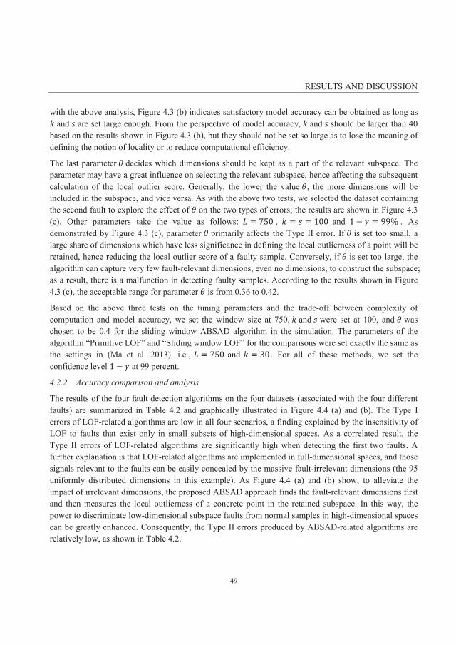
RESULTS AND DISCUSSION
49
with the above analysis, Figure 4.3 (b) indicates satisfactory model accuracy can be obtained as long as and are set large enough. From the perspective of model accuracy, and should be larger than 40 based on the results shown in Figure 4.3 (b), but they should not be set so large as to lose the meaning of defining the notion of locality or to reduce computational efficiency.
The last parameter decides which dimensions should be kept as a part of the relevant subspace. The parameter may have a great influence on selecting the relevant subspace, hence affecting the subsequent calculation of the local outlier score. Generally, the lower the value , the more dimensions will be included in the subspace, and vice versa. As with the above two tests, we selected the dataset containing the second fault to explore the effect of on the two types of errors; the results are shown in Figure 4.3 (c). Other parameters take the value as follows: = 750 , = = 100 and 1 = 99% . As demonstrated by Figure 4.3 (c), parameter primarily affects the Type II error. If is set too small, a large share of dimensions which have less significance in defining the local outlierness of a point will be retained, hence reducing the local outlier score of a faulty sample. Conversely, if is set too large, the algorithm can capture very few fault-relevant dimensions, even no dimensions, to construct the subspace; as a result, there is a malfunction in detecting faulty samples. According to the results shown in Figure 4.3 (c), the acceptable range for parameter is from 0.36 to 0.42.
Based on the above three tests on the tuning parameters and the trade-off between complexity of computation and model accuracy, we set the window size at 750, and were set at 100, and was chosen to be 0.4 for the sliding window ABSAD algorithm in the simulation. The parameters of the algorithm “Primitive LOF” and “Sliding window LOF” for the comparisons were set exactly the same as the settings in (Ma et al. 2013), i.e., = 750 and = 30 . For all of these methods, we set the confidence level 1 at 99 percent.
4.2.2 Accuracy comparison and analysis
The results of the four fault detection algorithms on the four datasets (associated with the four different faults) are summarized in Table 4.2 and graphically illustrated in Figure 4.4 (a) and (b). The Type I errors of LOF-related algorithms are low in all four scenarios, a finding explained by the insensitivity of LOF to faults that exist only in small subsets of high-dimensional spaces. As a correlated result, the Type II errors of LOF-related algorithms are significantly high when detecting the first two faults. A further explanation is that LOF-related algorithms are implemented in full-dimensional spaces, and those signals relevant to the faults can be easily concealed by the massive fault-irrelevant dimensions (the 95 uniformly distributed dimensions in this example). As Figure 4.4 (a) and (b) show, to alleviate the impact of irrelevant dimensions, the proposed ABSAD approach finds the fault-relevant dimensions first and then measures the local outlierness of a concrete point in the retained subspace. In this way, the power to discriminate low-dimensional subspace faults from normal samples in high-dimensional spaces can be greatly enhanced. Consequently, the Type II errors produced by ABSAD-related algorithms are relatively low, as shown in Table 4.2.

Results and discussion related to RQ 2
50
Table 4.2: Fault detection results of the numerical example
Dataset and error type Primitive LOF Sliding window LOF Primitive ABSAD Sliding window ABSAD Fault 1 Type I error 1.73a 1.73 8.4 0.67 Type II error 32.2 91.8 0.2 4.4 Fault 2 Type I error 2.4 3.73 8.4 0.8 Type II error 38.8 51 0 0 Fault 3 Type I error 2.8 2.27 8.13 1.2 Type II error 0 36.4 0 0 Fault 4 Type I error 2.13 1.87 8.8 0.67 Type II error 4.8 6.8 3.8 4.2 a Units of the decimal numbers in this table are in percentage (%)
The results in Table 4.2 also indicate that the primitive ABSAD has a higher level of Type I errors than does the sliding window ABSAD. By looking into the partially enlarged detail of Figure 4.4 (c), we can precisely locate the position of false alarms, i.e., where the blue line (local outlier score) exceeds the black dashed line (control limit). The reason for these false alarms is that the primitive ABSAD always holds the same window after the offline model training stage. The parameters of the model are invariant and thus cannot be adaptive to the time-varying behaviour of the system. Instead of keeping a constantly unchanged window, the sliding window ABSAD absorbs new samples, discards old samples regularly, and changes the window profile dynamically. As demonstrated by the partially enlarged detail in Figure 4.4 (d), the sliding window ABSAD algorithm adapts to the time-varying behaviour of the system very well with very few false alarms generated in the samples where the slow drift has been added.
Figure 4.4: Fault detection result of primitive LOF, sliding window LOF, primitive ABSAD and
sliding window ABSAD on scenario 2 of the numerical example
In the dataset containing the fourth fault, the degree of deviation of the fault from normal behaviour of the system is remarkably higher than that for the other three faults. Therefore, LOF-related algorithms can still produce desirable accuracy in terms of low Type I and Type II errors, as shown by Table 4.2 and Figure 4.5. It is worth noting that, according to Figure 4.5, there is a huge difference between the
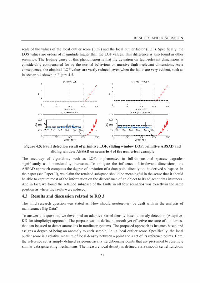
RESULTS AND DISCUSSION
51
scale of the values of the local outlier score (LOS) and the local outlier factor (LOF). Specifically, the LOS values are orders of magnitude higher than the LOF values. This difference is also found in other scenarios. The leading cause of this phenomenon is that the deviation on fault-relevant dimensions is considerably compensated for by the normal behaviour on massive fault-irrelevant dimensions. As a consequence, the obtained LOF values are vastly reduced, even when the faults are very evident, such as in scenario 4 shown in Figure 4.5.
Figure 4.5: Fault detection result of primitive LOF, sliding window LOF, primitive ABSAD and
sliding window ABSAD on scenario 4 of the numerical example
The accuracy of algorithms, such as LOF, implemented in full-dimensional spaces, degrades significantly as dimensionality increases. To mitigate the influence of irrelevant dimensions, the ABSAD approach computes the degree of deviation of a data point directly on the derived subspace. In the paper (see Paper II), we claim the retained subspace should be meaningful in the sense that it should be able to capture most of the information on the discordance of an object to its adjacent data instances. And in fact, we found the retained subspace of the faults in all four scenarios was exactly in the same position as where the faults were induced.
4.3 Results and discussion related to RQ 3 The third research question was stated as: How should nonlinearity be dealt with in the analysis of maintenance Big Data?
To answer this question, we developed an adaptive kernel density-based anomaly detection (Adaptive-KD for simplicity) approach. The purpose was to define a smooth yet effective measure of outlierness that can be used to detect anomalies in nonlinear systems. The proposed approach is instance-based and assigns a degree of being an anomaly to each sample, i.e., a local outlier score. Specifically, the local outlier score is a relative measure of local density between a point and a set of its reference points. Here, the reference set is simply defined as geometrically neighbouring points that are presumed to resemble similar data generating mechanisms. The measure local density is defined via a smooth kernel function.
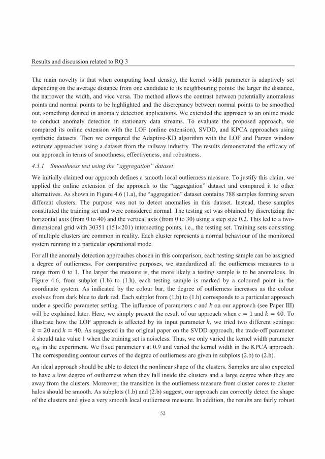
Results and discussion related to RQ 3
52
The main novelty is that when computing local density, the kernel width parameter is adaptively set depending on the average distance from one candidate to its neighbouring points: the larger the distance, the narrower the width, and vice versa. The method allows the contrast between potentially anomalous points and normal points to be highlighted and the discrepancy between normal points to be smoothed out, something desired in anomaly detection applications. We extended the approach to an online mode to conduct anomaly detection in stationary data streams. To evaluate the proposed approach, we compared its online extension with the LOF (online extension), SVDD, and KPCA approaches using synthetic datasets. Then we compared the Adaptive-KD algorithm with the LOF and Parzen window estimate approaches using a dataset from the railway industry. The results demonstrated the efficacy of our approach in terms of smoothness, effectiveness, and robustness.
4.3.1 Smoothness test using the “aggregation” dataset
We initially claimed our approach defines a smooth local outlierness measure. To justify this claim, we applied the online extension of the approach to the “aggregation” dataset and compared it to other alternatives. As shown in Figure 4.6 (1.a), the “aggregation” dataset contains 788 samples forming seven different clusters. The purpose was not to detect anomalies in this dataset. Instead, these samples constituted the training set and were considered normal. The testing set was obtained by discretizing the horizontal axis (from 0 to 40) and the vertical axis (from 0 to 30) using a step size 0.2. This led to a two-dimensional grid with 30351 (151 201) intersecting points, i.e., the testing set. Training sets consisting of multiple clusters are common in reality. Each cluster represents a normal behaviour of the monitored system running in a particular operational mode.
For all the anomaly detection approaches chosen in this comparison, each testing sample can be assigned a degree of outlierness. For comparative purposes, we standardized all the outlierness measures to a range from 0 to 1. The larger the measure is, the more likely a testing sample is to be anomalous. In Figure 4.6, from subplot (1.b) to (1.h), each testing sample is marked by a coloured point in the coordinate system. As indicated by the colour bar, the degree of outlierness increases as the colour evolves from dark blue to dark red. Each subplot from (1.b) to (1.h) corresponds to a particular approach under a specific parameter setting. The influence of parameters and on our approach (see Paper III) will be explained later. Here, we simply present the result of our approach when = 1 and = 40. To illustrate how the LOF approach is affected by its input parameter , we tried two different settings: = 20 and = 40. As suggested in the original paper on the SVDD approach, the trade-off parameter
should take value 1 when the training set is noiseless. Thus, we only varied the kernel width parameter rbf in the experiment. We fixed parameter at 0.9 and varied the kernel width in the KPCA approach. The corresponding contour curves of the degree of outlierness are given in subplots (2.b) to (2.h).
An ideal approach should be able to detect the nonlinear shape of the clusters. Samples are also expected to have a low degree of outlierness when they fall inside the clusters and a large degree when they are away from the clusters. Moreover, the transition in the outlierness measure from cluster cores to cluster halos should be smooth. As subplots (1.b) and (2.b) suggest, our approach can correctly detect the shape of the clusters and give a very smooth local outlierness measure. In addition, the results are fairly robust
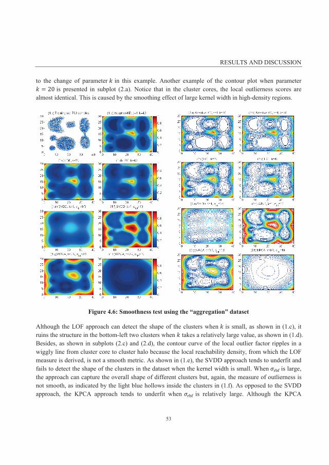
RESULTS AND DISCUSSION
53
to the change of parameter in this example. Another example of the contour plot when parameter = 20 is presented in subplot (2.a). Notice that in the cluster cores, the local outlierness scores are almost identical. This is caused by the smoothing effect of large kernel width in high-density regions.
Figure 4.6: Smoothness test using the “aggregation” dataset
Although the LOF approach can detect the shape of the clusters when is small, as shown in (1.c), it ruins the structure in the bottom-left two clusters when takes a relatively large value, as shown in (1.d). Besides, as shown in subplots (2.c) and (2.d), the contour curve of the local outlier factor ripples in a wiggly line from cluster core to cluster halo because the local reachability density, from which the LOF measure is derived, is not a smooth metric. As shown in (1.e), the SVDD approach tends to underfit and fails to detect the shape of the clusters in the dataset when the kernel width is small. When rbf is large, the approach can capture the overall shape of different clusters but, again, the measure of outlierness is not smooth, as indicated by the light blue hollows inside the clusters in (1.f). As opposed to the SVDD approach, the KPCA approach tends to underfit when rbf is relatively large. Although the KPCA
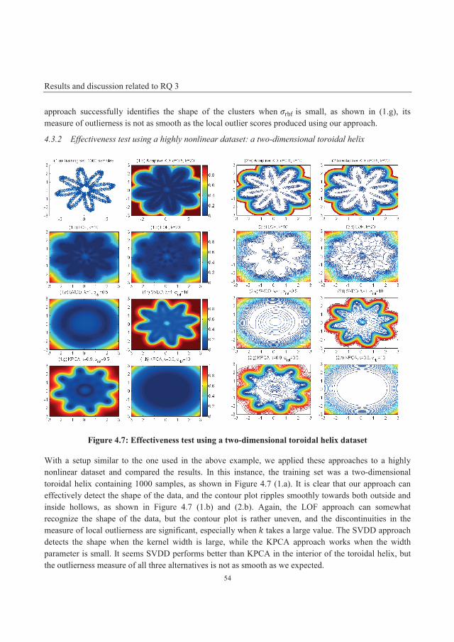
Results and discussion related to RQ 3
54
approach successfully identifies the shape of the clusters when rbf is small, as shown in (1.g), its measure of outlierness is not as smooth as the local outlier scores produced using our approach.
4.3.2 Effectiveness test using a highly nonlinear dataset: a two-dimensional toroidal helix
Figure 4.7: Effectiveness test using a two-dimensional toroidal helix dataset
With a setup similar to the one used in the above example, we applied these approaches to a highly nonlinear dataset and compared the results. In this instance, the training set was a two-dimensional toroidal helix containing 1000 samples, as shown in Figure 4.7 (1.a). It is clear that our approach can effectively detect the shape of the data, and the contour plot ripples smoothly towards both outside and inside hollows, as shown in Figure 4.7 (1.b) and (2.b). Again, the LOF approach can somewhat recognize the shape of the data, but the contour plot is rather uneven, and the discontinuities in the measure of local outlierness are significant, especially when takes a large value. The SVDD approach detects the shape when the kernel width is large, while the KPCA approach works when the width parameter is small. It seems SVDD performs better than KPCA in the interior of the toroidal helix, but the outlierness measure of all three alternatives is not as smooth as we expected.

RESULTS AND DISCUSSION
55
As we varied parameter while fixing in our approach, the results could appear to be over-smoothing or under-smoothing because the kernel width defined in our approach is also affected by parameter . In general, a small will lead to a small kernel width, thereby decreasing the overall smoothing effect. The phenomenon can be compensated for by choosing a larger . In Figure 4.7 (2.a), we present another comparable result; in this example, = 0.8 and = 10 . The effect of over-smoothing and under-smoothing is elaborated in detail in the next subsection.
In the above two examples, our purpose was to compare our approach with selected alternatives. Even though a global measure of outlierness derived from a well-tuned kernel density estimator can achieve comparable smoothness in these examples, it may fail in a dataset where clusters have significant differences in their densities, as we argued in Subsection 2.6.1.
4.3.3 Robustness test using the “flame” dataset
In the following, we describe our use of the “flame” dataset to determine how the existence of anomalies in the training set affects the various approaches. We also discuss the robustness of our approach to the perturbation of input parameters. The “flame” dataset is shown in Figure 4.8 (1.a); the top-left-most two points are considered anomalies. The remaining sub-graphs in Figure 4.8 agree with our assessment of the smoothness and effectiveness of the approaches in the previous two examples. They also demonstrate that all approaches are affected by the two anomalies, albeit to a different extent. The Adaptive-KD approach naturally has the ability to assign a local outlier score to any sample in the training set. Thus, the data refinement step in the offline training stage should be able to capture and discard these two anomalies and retrain a model on the refined set. The LOF approach can recognize the two anomalies using the same routine. However, it is non-trivial for the SVDD and KPCA approaches to mitigate the effect exerted by anomalies in the training set.
The impacts on our approach of perturbing the input parameters are shown in Figure 4.9. First, we varied parameter while fixing ; the results are shown in (1.a) and (1.b), and the corresponding contour plots are given in (2.a) and (2.b). As expected, parameter directly controls the overall smoothing effect. A small may cause the fine details in the data to be enhanced, leading to overfitting, whereas a large one may lead to over-smoothing and underfitting. Note that when a large is chosen, the influence of anomalies in the training set can be somewhat counteracted because the local information at the two anomalies is smoothed out. Second, we varied parameter while fixing ; the results are shown in (1.c) and (1.d), and the corresponding contour plots are given in (2.c) and (2.d). Unsurprisingly, since parameter has an indirect influence on the scale of kernel width, it can affect the smoothing effect in a manner similar to . The main difference is that also decides the number of reference sets and consequently affects the local outlierness measure. This explains why the contour plot shown in (2.c) has a very wiggly interior when takes a small value.
Results and discussion related to RQ 3
56
Figure 4.8: Robustness test on the existence of anomalies in the training set
As with other unsupervised learning approaches, the Adaptive-KD approach relies on the similarity (or dissimilarity) measure between points. Specifically, the measure computes how similar one point’s local density is to the densities of its nearest neighbours. In an extreme case, when takes the value of the size of the training set, the measure recovers to a global measure of outlierness, and the rank in the outlierness measure is simply the rank in the metric local density in reverse order. If takes a very small value, however, the local densities of the very few reference points may dominate the calculation of the point’s local outlier score, thereby leading to discontinuities in the outlierness measure, as shown in Figure 4.9 (2.c). According to our experiments in the above three examples, the results are fairly robust to changes in parameter as long as it does not fall into too large or too small a range. Thus, we recommend setting to a reasonably small value in order to capture the notion of locality and then adjusting accordingly. Although the purpose of anomaly detection differs from that of density estimation, some heuristic methods (such as minimizing the frequentist risk) in density estimation applications can be employed to make a preliminary selection of parameter .
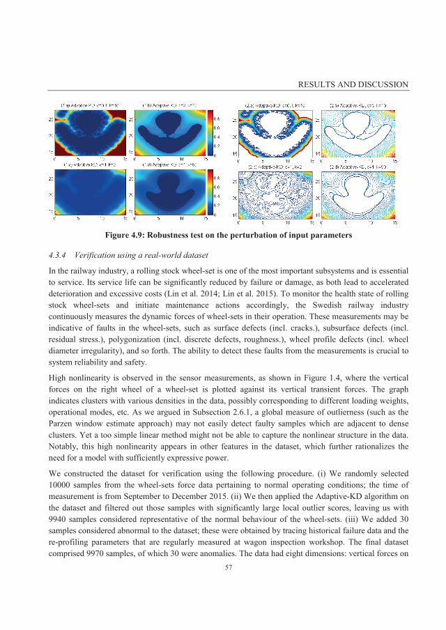
RESULTS AND DISCUSSION
57
Figure 4.9: Robustness test on the perturbation of input parameters
4.3.4 Verification using a real-world dataset
In the railway industry, a rolling stock wheel-set is one of the most important subsystems and is essential to service. Its service life can be significantly reduced by failure or damage, as both lead to accelerated deterioration and excessive costs (Lin et al. 2014; Lin et al. 2015). To monitor the health state of rolling stock wheel-sets and initiate maintenance actions accordingly, the Swedish railway industry continuously measures the dynamic forces of wheel-sets in their operation. These measurements may be indicative of faults in the wheel-sets, such as surface defects (incl. cracks.), subsurface defects (incl. residual stress.), polygonization (incl. discrete defects, roughness.), wheel profile defects (incl. wheel diameter irregularity), and so forth. The ability to detect these faults from the measurements is crucial to system reliability and safety.
High nonlinearity is observed in the sensor measurements, as shown in Figure 1.4, where the vertical forces on the right wheel of a wheel-set is plotted against its vertical transient forces. The graph indicates clusters with various densities in the data, possibly corresponding to different loading weights, operational modes, etc. As we argued in Subsection 2.6.1, a global measure of outlierness (such as the Parzen window estimate approach) may not easily detect faulty samples which are adjacent to dense clusters. Yet a too simple linear method might not be able to capture the nonlinear structure in the data. Notably, this high nonlinearity appears in other features in the dataset, which further rationalizes the need for a model with sufficiently expressive power.
We constructed the dataset for verification using the following procedure. (i) We randomly selected 10000 samples from the wheel-sets force data pertaining to normal operating conditions; the time of measurement is from September to December 2015. (ii) We then applied the Adaptive-KD algorithm on the dataset and filtered out those samples with significantly large local outlier scores, leaving us with 9940 samples considered representative of the normal behaviour of the wheel-sets. (iii) We added 30 samples considered abnormal to the dataset; these were obtained by tracing historical failure data and the re-profiling parameters that are regularly measured at wagon inspection workshop. The final dataset comprised 9970 samples, of which 30 were anomalies. The data had eight dimensions: vertical forces on
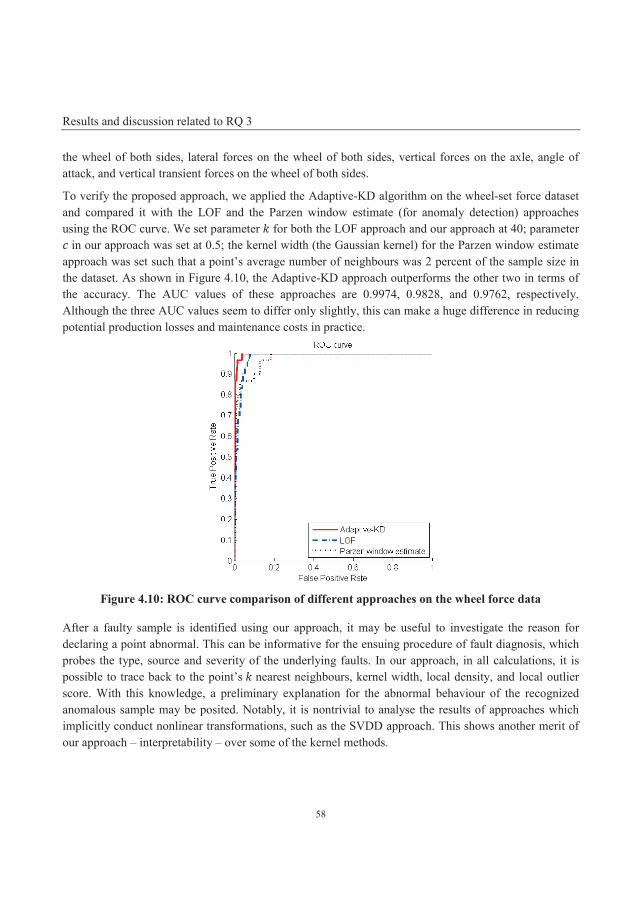
Results and discussion related to RQ 3
58
the wheel of both sides, lateral forces on the wheel of both sides, vertical forces on the axle, angle of attack, and vertical transient forces on the wheel of both sides.
To verify the proposed approach, we applied the Adaptive-KD algorithm on the wheel-set force dataset and compared it with the LOF and the Parzen window estimate (for anomaly detection) approaches using the ROC curve. We set parameter for both the LOF approach and our approach at 40; parameter in our approach was set at 0.5; the kernel width (the Gaussian kernel) for the Parzen window estimate
approach was set such that a point’s average number of neighbours was 2 percent of the sample size in the dataset. As shown in Figure 4.10, the Adaptive-KD approach outperforms the other two in terms of the accuracy. The AUC values of these approaches are 0.9974, 0.9828, and 0.9762, respectively. Although the three AUC values seem to differ only slightly, this can make a huge difference in reducing potential production losses and maintenance costs in practice.
Figure 4.10: ROC curve comparison of different approaches on the wheel force data
After a faulty sample is identified using our approach, it may be useful to investigate the reason for declaring a point abnormal. This can be informative for the ensuing procedure of fault diagnosis, which probes the type, source and severity of the underlying faults. In our approach, in all calculations, it is possible to trace back to the point’s nearest neighbours, kernel width, local density, and local outlier score. With this knowledge, a preliminary explanation for the abnormal behaviour of the recognized anomalous sample may be posited. Notably, it is nontrivial to analyse the results of approaches which implicitly conduct nonlinear transformations, such as the SVDD approach. This shows another merit of our approach – interpretability – over some of the kernel methods.
RESULTS AND DISCUSSION
59
4.3.5 Time complexity analysis
In this section we discuss the time complexity of the Adaptive-KD algorithm and its online extension. The most computationally intensive steps in the algorithm are the derivation of nearest neighbours and the computation of local density, both of which take the time complexity of ( max ( , )), where , , and denote the number of samples, dimensions and nearest neighbours, respectively. Thus, the overall time complexity for the primitive Adaptive-KD algorithm and the offline model training phase (assuming there are data points in the training set) of its extension are ( max ( , )). It is possible to reduce the computational cost by applying the following considerations to the above two steps.
Choosing locality dependent kernel width is better than choosing a uniformly constant kernel width, but this increases the computational complexity of performing local density evaluation, as it requires finding
nearest neighbours before figuring out the kernel width of points. A typical way to reduce the time complexity of finding nearest neighbours is to employ an indexing structure, such as - tree or R tree. The time complexity can be reduced to ( log ( ) max ( , )) at the expense of additional memory space. Another improvement, random projection, can alleviate the high computational cost of finding nearest neighbours when the dimensionality is high. This is supported by the Johnson-Lindenstrauss theorem claiming that a set of points in a high-dimensional Euclidean space can be embedded into a (log ( / )) dimensional Euclidean space such that any pairwise distance changes only by a factor of (1 ± ) (Dasgupta & Gupta 2003).
The complication of local density computation lies in the Gaussian kernel evaluation, mainly because the Gaussian kernel has an unbounded support. In other words, the Gaussian kernel function needs to be evaluated for each point with respect to all remaining points. While the shape of the kernel function may be important in theoretical research, from a practical perspective, it matters far less than the width parameter. Thus, other kernel functions with compact support, such as the Epanechnikov or the Tri-cube kernel, can be adopted. However, they require introducing additional parameters to determine the size of their support. Typically, only those points with a distance less than a given threshold to the point of interest will be evaluated using the chosen kernel function.
The online testing phase of the algorithm’s extension continuously processes new samples upon their arrival. The time complexity of this phase is much more important in the sense that it decides whether the algorithm can give real-time or near real-time responses to a fast-flowing data stream. It is necessary to maintain those model parameters yielded from the training phase to avoid repetitive computations at testing time. This is where the concept of trading space for time applies. As in the offline model training phase, the most computationally demanding steps in the online testing phase are the derivation of nearest neighbours and the computation of local density, both of which have a time complexity of (max ( , )). With the same considerations as previously discussed, the computational cost can be vastly reduced.

60
61
CHAPTER 5. CONCLUSIONS, CONTRIBUTIONS AND FUTURE RESEARCH
This chapter concludes the research, summarizes the contributions and suggests future research.
5.1 Conclusions Based on the results of this research, the following answers have been found for, the three research questions (RQs) given in Chapter 1.
RQ 1: How can patterns be extracted from maintenance Big Data with high dimensionality characteristics?
The proposed ABSAD approach can select meaningful subspaces from the original high-dimensional space. In other words, it can retain dimensions which present a large discrepancy between points and their neighbouring points.
The analytical study proves the metric “pairwise cosine” is a bounded metric when it is used to measure vectorial angles in high-dimensional spaces, and it becomes asymptotically stable as dimensionality increases.
The experiments on synthetic datasets with various dimensionality settings indicate the suggested algorithm can detect anomalies effectively and has superior accuracy when compared to the specified alternatives in high-dimensional spaces.
The experiment on the industrial dataset shows the applicability of the algorithm in real-world fault detection applications; in addition, its feature ordering in relevant subspaces is informative to the ensuing analysis and diagnosis of abnormality.
RQ 2: How should high-dimensional data streams be dealt with in the analysis of maintenance Big Data?
The experiments on synthetic datasets indicate the ABSAD approach has the ability to discriminate low-dimensional subspace faults from normal samples in high-dimensional spaces. Moreover, it outperforms the Local Outlier Factor (LOF) approach in the context of high-dimensional fault detection.
CONCLUSIONS, CONTRIBUTIONS AND FUTURE RESEARCH
62
The experiments on synthetic datasets further demonstrate that the sliding window ABSAD algorithm can be adaptive to the time-varying behaviour of the monitored system and produce better accuracy than the primitive ABSAD algorithm even when the monitored system has time-varying characteristics.
By applying the concept of trading space for time, the sliding window ABSAD algorithm can isochronously perform online fault detection.
RQ 3: How should nonlinearity be dealt with in the analysis of maintenance Big Data?
The Adaptive-KD approach is able to recognize nonlinear structures in the data.
The experiments on synthetic datasets demonstrate that the proposed local outlier score is a smooth measure. Further, local outlier scores of points in cluster cores are nearly identical, and those in cluster halos are significantly larger. This indicates the locality dependent kernel width can enhance the power to discriminate in anomaly detection tasks.
Analytical study shows that the online extension of the proposed approach is more robust to the existence of anomalies in the training set with the data refinement step. It is also more robust to changes in parameter than is the LOF approach.
The interpretability of the approach is much greater than other kernel methods which implicitly conduct nonlinear transformations from the input space to a feature space.
The experiment on the industrial dataset shows the applicability of the algorithm in real-world applications.
5.2 Research contributions The main contributions of this research can be summarized as follows:
A novel Angle-based Subspace Anomaly Detection (ABSAD) approach to high-dimensional data has been developed. The approach can be applied in industrial fault detection in high-dimensional circumstances.
The ABSAD approach has been extended to an online mode based on the sliding window strategy. The extension can be applied to online fault detection in a dynamic environment.
A novel Adaptive Kernel Density-based (Adaptive-KD) anomaly detection approach to nonlinear data has been developed. The approach has been extended to an online mode with the purpose of detecting faults from stationary, nonlinear data streams. The approach has been found superior in terms of smoothness, effectiveness, robustness, and interpretability.
5.3 Future research The following are considered interesting topic for future research.
Given the output of the ABSAD approach in fault detection applications, methods like case-based reasoning may be adopted to conduct fault diagnosis.

CONCLUSIONS, CONTRIBUTIONS AND FUTURE RESEARCH
63
The Adaptive-KD approach can be extended to detect faults in non-stationary data streams in a temporal context, using, for example, the sliding window strategy.
The approaches proposed in this research can be applied to other real-world applications to verify their merits and discover and solve any shortcomings.

64

65
REFERENCES
Aggarwal, C.C. et al., 2005. On high dimensional projected clustering of data streams. Data Mining and Knowledge Discovery, 10(3), pp.251–273.
Aggarwal, C.C. & Yu, P.S., 2001. Outlier detection for high dimensional data. ACM SIGMOD Record, 30(2), pp.37–46.
Agovic, A. et al., 2009. Anomaly detection using manifold embedding and its applications in transportation corridors. Intelligent Data Analysis, 13(3), pp.435–455.
Ahmad, R. & Kamaruddin, S., 2012. A review of condition-based maintenance decision-making. European journal of industrial engineering, 6(5), pp.519–541.
Ajami, A. & Daneshvar, M., 2012. Data driven approach for fault detection and diagnosis of turbine in thermal power plant using Independent Component Analysis (ICA). International Journal of Electrical Power & Energy Systems, 43(1), pp.728–735.
Albaghdadi, M., Briley, B. & Evens, M., 2006. Event storm detection and identification in communication systems. Reliability Engineering & System Safety, 91(5), pp.602–613.
Alippi, C., Roveri, M. & Trovò, F., 2014. A self-building and cluster-based cognitive fault diagnosis system for sensor networks. IEEE Transactions on Neural Networks and Learning Systems, 25(6), pp.1021–1032.
Alzghoul, A. & Löfstrand, M., 2011. Increasing availability of industrial systems through data stream mining. Computers & Industrial Engineering, 60(2), pp.195–205.
Amari, S.V., McLaughlin, L. & Pham, H., 2006. Cost-effective condition-based maintenance using markov decision processes. Annual Reliability and Maintainability Symposium, 2006 (RAMS ’06)., pp.464–469.
Apache, Spark. Available at: https://spark.apache.org/ [Accessed October 7, 2016].
Bahga, A. & Madisetti, V.K., 2012. Analyzing massive machine maintenance data in a computing cloud. IEEE Transactions on Parallel and Distributed Systems, 23(10), pp.1831–1843.
Baraldi, P., Razavi-Far, R. & Zio, E., 2011. Classifier-ensemble incremental-learning procedure for nuclear transient identification at different operational conditions. Reliability Engineering & System

REFERENCES
66
Safety, 96(4), pp.480–488.
Bell, C.G., Hey, T. & Szalay, A.S., 2009. COMPUTER SCIENCE: Beyond the Data Deluge. Science, 323(5919), pp.1297–1298.
Beyer, K. et al., 1999. When is “nearest neighbor” meaningful? In Database Theory—ICDT’99. Springer Berlin Heidelberg, pp. 217–235.
Beyer, M.A. & Laney, D., 2012. The Importance of “Big Data”: A Definition. Stamford, CT: Gartner.
Bishop, C.M., 2006. Pattern Recognition and Machine Learning 1st ed., Springer-Verlag New York.
Bloch, H.P. & Geitner, F.K., 2012. Machinery Failure Analysis and Troubleshooting: Practical Machinery Management for Process Plants 4th ed., Oxford, UK: Butterworth-Heinemann.
Breunig, M.M. et al., 2000. -Based Local Outliers. ACM Sigmod Record., 29(2), pp.93–104.
Campbell, C., 2002. Kernel methods: a survey of current techniques. Neurocomputing, 42, pp.63–84.
CEN, C.E.D.., 2010. EN 13306: Maintenance - maintenance terminology, Brussels.
Chandola, V., Banerjee, A. & Kumar, V., 2009. Anomaly detection: A survey. ACM Computing Surveys (CSUR), 41(3), pp.1–72.
Chandola, V., Banerjee, A. & Kumar, V., 2012. Anomaly Detection for Discrete Sequences: A Survey. IEEE Transactions on Knowledge and Data Engineering, 24(5), pp.823–839.
Chen, C.L.P. & Zhang, C.Y., 2014. Data-intensive applications, challenges, techniques and technologies: A survey on Big Data. Information Sciences, 275, pp.314–347.
Chen, H., Chiang, R.H.L. & Storey, V.C., 2012. Business Intelligence and Analytics: From Big Data To Big Impact. Mis Quarterly, 36(4), pp.1165–1188.
Creswell, J.W., 2013. Research design: Qualitative, quantitative, and mixed methods approaches, Sage publications.
Dai, X. & Gao, Z., 2013. From model, signal to knowledge: a data-driven perspective of fault detection and diagnosis. IEEE Transactions on Industrial Informatics, 9(4), pp.2226–2238.
Dasgupta, S. & Gupta, A., 2003. An Elementary Proof of a Theorem of Johnson and Lindenstrauss. Random Structures and Algorithms, 22(1), pp.60–65.
Domingos, P., 2012. A few useful things to know about machine learning. Communications of the ACM, 55(10), pp.78–87.
Eriksson, L. et al., 2001. Multivariate process monitoring of a newsprint mill. Application to modelling and predicting COD load resulting from de-inking of recycled paper. Journal of Chemometrics, 15(4), pp.337–352.
Fumeo, E., Oneto, L. & Anguita, D., 2015. Condition Based Maintenance in Railway Transportation
REFERENCES
67
Systems Based on Big Data Streaming Analysis. Procedia Computer Science, 53, pp.437–446.
Gao, J. et al., 2008. Classifying data streams with skewed class distributions and concept drifts. IEEE Internet Computing, 12(6), pp.37–49.
Ge, Z. & Song, Z., 2007. Process monitoring based on independent component analysis-principal component analysis (ICA-PCA) and similarity factors. Industrial & Engineering Chemistry Research, 46(7), pp.2054–2063.
Gehrke, J., 2009. Technical perspective Data stream Processing— When You only Get one Look. Communications of the ACM, 52(10), pp.96–96.
Göb, R., 2013. Discussion of “Reliability Meets Big Data: Opportunities and Challenges.” Quality Engineering, 26(1), pp.121–126.
Hawkins, D.M., 1980. Identification of outliers, London: Chapman and Hall.
Holmberg, K. et al., 2010. Information and Communication Technologies Within E-maintenance. In E-maintenance. Springer Science & Business Media, pp. 39–60.
Houle, M.E. et al., 2010. Can shared-neighbor distances defeat the curse of dimensionality? In Scientific and Statistical Database Management. Springer Berlin Heidelberg, pp. 482–500.
Huang, G.-B., Wang, D.H. & Lan, Y., 2011. Extreme learning machines: A survey. International Journal of Machine Learning and Cybernetics, 2(2), pp.107–122.
Hwang, W.-Y. & Lee, J.-S., 2015. Shifting artificial data to detect system failures. International Transactions in Operational Research, 22(2), pp.363–378.
Iung, B. & Marquez, A.C., 2006. Special issue on e-maintenance. Computers in Industry, 57(6), pp.473–475.
Jagadish, H. V. et al., 2014. Big Data and Its Technical Challenges. Communications of the ACM, 57(7), pp.86–94.
Jardine, A.K.S., Lin, D. & Banjevic, D., 2006. A review on machinery diagnostics and prognostics implementing condition-based maintenance. Mechanical Systems and Signal Processing, 20(7), pp.1483–1510.
Jeng, J.-C., 2010. Adaptive process monitoring using efficient recursive PCA and moving window PCA algorithms. Journal of the Taiwan Institute of Chemical Engineers, 41(4), pp.475–481.
Kajko-Mattsson, M., Karim, R. & Mirjamdotter, A., 2011. Essential Components of e-Maintenance. International Journal of Performability Engineering, 7(6), pp.555–571.
Karim, R., Candell, O. & Söderholm, P., 2009. E-maintenance and information logistics: aspects of content format. Journal of Quality in Maintenance Engineering, 15(3), pp.308–324.
Kim, J. & Scott, C.D., 2012. Robust Kernel Density Estimation. Journal of Machine Learning Research, 13(Sep), pp.2529–2565.

REFERENCES
68
Knorr, E.M., Ng, R.T. & Tucakov, V., 2000. Distance-based outliers: algorithms and applications. The VLDB Journal The International Journal on Very Large Data Bases, 8(3–4), pp.237–253.
Koc, M. & Lee, J., 2003. E-manufacturing-fundamentals, requirements and expected impacts. International Journal of Advanced Manufacturing Systems, 6(1), pp.29–46.
Kothamasu, R., Huang, S.H. & VerDuin, W.H., 2009. System health monitoring and prognostics—a review of current paradigms and practices. In Handbook of Maintenance Management and Engineering. Springer London, pp. 337–362.
Kothari, C.R., 2011. Research methodology: methods and techniques, New Age International.
Krawczyk, B., Wozniak, M. & Stefanowski, J., 2015. Data stream classification and big data analytics. Neurocomputing, 150(May 2013), pp.238–239.
Kriegel, H.-P. et al., 2009. Outlier detection in axis-parallel subspaces of high dimensional data. In Advances in Knowledge Discovery and Data Mining. Springer Berlin Heidelberg, pp. 831–838.
Kriegel, H.-P. & Zimek, A., 2008. Angle-based outlier detection in high-dimensional data. Proceeding of the 14th ACM SIGKDD international conference on Knowledge discovery and data mining, pp.444–452.
Lane, S. et al., 2003. Application of exponentially weighted principal component analysis for the monitoring of a polymer film manufacturing process. Transactions of the Institute of Measurement and Control, 25(1), pp.17–35.
Lazarevic, A. & Kumar, V., 2005. Feature bagging for outlier detection. In Proceeding of the eleventh ACM SIGKDD international conference on Knowledge discovery in data mining. New York, USA: ACM Press, pp. 157–166.
Lee, J., Kang, B. & Kang, S.-H., 2011. Integrating independent component analysis and local outlier factor for plant-wide process monitoring. Journal of Process Control, 21(7), pp.1011–1021.
Lee, J.-M., Qin, S.J. & Lee, I.-B., 2006. Fault detection and diagnosis based on modified independent component analysis. AIChE Journal, 52(10), pp.3501–3514.
Levrat, E., Iung, B. & Marquez, A.C., 2008. E-maintenance: review and conceptual framework. Production Planning & Control, 19(4), pp.408–429.
Li, J. et al., 2008. A survey on statistical methods for health care fraud detection. Health Care Management Science, 11(3), pp.275–287.
Li, W. et al., 2000. Recursive PCA for adaptive process monitoring. Journal of Process Control, 10(5), pp.471–486.
Lin, J., Asplunda, M. & Parida, A., 2014. Reliability analysis for degradation of locomotive wheels using parametric bayesian approach. Quality and Reliability Engineering International, 30(5), pp.657–667.
REFERENCES
69
Lin, J., Pulido, J. & Asplund, M., 2015. Reliability analysis for preventive maintenance based on classical and Bayesian semi-parametric degradation approaches using locomotive wheel-sets as a case study. Reliability Engineering and System Safety, 134, pp.143–156.
Ma, Y. et al., 2013. Dynamic process monitoring using adaptive local outlier factor. Chemometrics and Intelligent Laboratory Systems, 127, pp.89–101.
Manyika, J. et al., 2011. Big data: The next frontier for innovation, competition, and productivity. McKinsey Global Institute, (June), p.156.
Meeker, W.Q. & Hong, Y., 2014. Reliability meets big data: Opportunities and challenges. Quality Engineering, 26(1), pp.102–116.
Montgomery, D.C., 2014. Big Data and the Quality Profession. Quality and Reliability Engineering International, 30(4), pp.447–447.
Murphy, K.P., 2012. Machine learning: a probabilistic perspective 1st ed., MIT Press.
Müller, E., Schiffer, M. & Seidl, T., 2010. Adaptive outlierness for subspace outlier ranking. In Proceedings of the 19th ACM international conference on Information and knowledge management. New York, USA: ACM Press, pp. 1629–1632.
Müller, E., Schiffer, M. & Seidl, T., 2011. Statistical selection of relevant subspace projections for outlier ranking. In Data Engineering (ICDE), 2011 IEEE 27th International Conference on. IEEE, pp. 434–445.
Nowicki, A., Grochowski, M. & Duzinkiewicz, K., 2012. Data-driven models for fault detection using kernel PCA: A water distribution system case study. International Journal of Applied Mathematics and Computer Science, 22(4), pp.939–949.
Olken, F. & Gruenwald, L., 2008. Data Stream Management: Aggregation, Classification, Modeling, and Operator Placement. IEEE Internet Computing, 6, pp.9–12.
PAS, 55-1:2008, Asset Management Part 1: Specification for the optimized management of physical assets. BSI, UK.
Patcha, A. & Park, J.-M., 2007. An overview of anomaly detection techniques: Existing solutions and latest technological trends. Computer Networks, 51(12), pp.3448–3470.
Peng, Y., Dong, M. & Zuo, M.J., 2010. Current status of machine prognostics in condition-based maintenance: A review. International Journal of Advanced Manufacturing Technology, 50(1–4), pp.297–313.
Percy, D.F. & Kobbacy, K.A.H., 2000. Determining economical maintenance intervals. International Journal of Production Economics, 67(1), pp.87–94.
Piao, C. et al., 2014. Research on Outlier Detection Algorithm for Evaluation of Battery System Safety. Advances in Mechanical Engineering, 2014, pp.1–8.

REFERENCES
70
Rao, B.K.N., 1996. The need for condition monitoring and maintenance management in industries. In Handbook of condition monitoring. Amsterdam: Elsevier, pp. 1–36.
Rocco S., C.M. & Zio, E., 2007. A support vector machine integrated system for the classification of operation anomalies in nuclear components and systems. Reliability Engineering & System Safety, 92(5), pp.593–600.
Rosmaini, A. & Kamaruddin, S., 2012. An overview of time-based and condition-based maintenance in industrial application. Computers and Industrial Engineering, 63(1), pp.135–149.
Roweis, S.T. & Saul, L.K., 2000. Nonlinear Dimensionality Reduction by Locally Linear Embedding. Science, 290(5500), pp.2323–2326.
Schubert, E., Zimek, A. & Kriegel, H.-P., 2014. Local outlier detection reconsidered: A generalized view on locality with applications to spatial, video, and network outlier detection. Data Mining and Knowledge Discovery, 28(1), pp.190–237.
Sribar, V. et al., 2011. Big Data is only the beginning of extreme information management. Gartner, Stamford, CT.
Journal of Machine Learning Research (JMLR), 15, pp.1929–1958.
Sun, C. et al., 2015. A non-probabilistic metric derived from condition information for operational reliability assessment of aero-engines. IEEE Transactions on Reliability, 64(1), pp.167–181.
Swearingen, K. et al., 2007. An Open System Architecture for Condition Based Maintenance Overview. 2007 IEEE Aerospace Conference, pp.1–8.
Tamilselvan, P. & Wang, P., 2013. Failure diagnosis using deep belief learning based health state classification. Reliability Engineering & System Safety, 115, pp.124–135.
Tax, D.M.J. & Duin, R.P.W., 2004. Support Vector Data Description. Machine Learning, 54(1), pp.45–66.
Tenenbaum, J.B., Silva, V. De & Langford, J.C., 2000. A Global Geometric Framework for Nonlinear Dimensionality Reduction. Science, 290(5500), pp.2319–2323.
Traore, M., Chammas, A. & Duviella, E., 2015. Supervision and prognosis architecture based on dynamical classification method for the predictive maintenance of dynamical evolving systems. Reliability Engineering & System Safety, 136, pp.120–131.
Vaidya, P. & Rausand, M., 2011. Remaining useful life, technical health, and life extension. Proceedings of the Institution of Mechanical Engineers, Part O: Journal of Risk and Reliability, 225(2), pp.219–231.
Warren, P.W. & Davies, N.J., 2007. Managing the risks from information — through semantic information management. BT Technology Journal, 25(1), pp.178–191.
REFERENCES
71
Verleysen, M. & François, D., 2005. The Curse of Dimensionality in Data Mining and Time Series Prediction. In Computational Intelligence and Bioinspired Systems. Springer Berlin Heidelberg, pp. 758–770.
Wu, X. et al., 2014. Data mining with big data. Knowledge and Data Engineering, IEEE Transactions on, 26(1).
Ye, M., Li, X. & Orlowska, M.E., 2009. Projected outlier detection in high-dimensional mixed-attributes data set. Expert Systems with Applications, 36(3), pp.7104–7113.
Yu, H., Khan, F. & Garaniya, V., 2015. Risk-based fault detection using Self-Organizing Map. Reliability Engineering & System Safety, 139, pp.82–96.
Yu, J., 2012. A nonlinear kernel Gaussian mixture model based inferential monitoring approach for fault detection and diagnosis of chemical processes. Chemical Engineering Science, 68(1), pp.506–519.
Zhai, Y., Ong, Y.-S. & Tsang, I.W., 2014. The Emerging “Big Dimensionality.” Computational Intelligence Magazine, IEEE, 9(3), pp.14–26.
Proceedings of the 3rd international workshop and congress on eMaintenance. universitet, pp. 159–170.
Zhang, L., Lin, J. & Karim, R., 2015. An angle-based subspace anomaly detection approach to high-dimensional data: With an application to industrial fault detection. Reliability Engineering & System Safety, 142, pp.482–497.
Zhang, L., Lin, J. & Karim, R., 2016. Sliding Window-Based Fault Detection from High-Dimensional Data Streams. IEEE Transactions on Systems, Man, and Cybernetics: Systems, (doi: 10.1109/TSMC.2016.2585566). Available at: http://ieeexplore.ieee.org/document/7509594/.
Zhang, Y., Meratnia, N. & Havinga, P., 2010. Outlier Detection Techniques for Wireless Sensor Networks: A Survey. IEEE Communications Surveys & Tutorials, 12(2), pp.159–170.
Zhao, Y., Wang, S. & Xiao, F., 2013. Pattern recognition-based chillers fault detection method using Support Vector Data Description (SVDD). Applied Energy, 112, pp.1041–1048.
Zhong, S., Langseth, H. & Nielsen, T.D., 2014. A classification-based approach to monitoring the safety of dynamic systems. Reliability Engineering & System Safety, 121, pp.61–71.
Zhu, X. et al., 2010. Active learning from stream data using optimal weight classifier ensemble. IEEE Transactions on Systems, Man, and Cybernetics, Part B: Cybernetics, 40(6), pp.1607–1621.
Zimek, A., Schubert, E. & Kriegel, H.-P., 2012. A survey on unsupervised outlier detection in high-dimensional numerical data. Statistical Analysis and Data Mining, 5(5), pp.363–387.
Zou, W.Y. et al., 2012. Deep Learning of Invariant Features via Simulated Fixations in Video. Advances in Neural Information Processing Systems, pp.3212–3220.

72
PAPER I
An Angle-based Subspace Anomaly Detection Approach to
High-dimensional Data: With an Application to Industrial
Fault Detection
Zhang, L., Lin, J. and Karim, R., 2015. An Angle-based Subspace Anomaly Detection Approach to
High-dimensional Data: With an Application to Industrial Fault Detection. Reliability Engineering &
System Safety, 142, pp.482-497.
http://dx.doi.org/10.1016/j.ress.2015.05.025

An angle-based subspace anomaly detection approachto high-dimensional data: With an applicationto industrial fault detection
Liangwei Zhang n, Jing Lin, Ramin KarimDivision of Operation and Maintenance Engineering, Luleå University of Technology, 97187 Luleå, Sweden
a r t i c l e i n f o
Article history:Received 11 February 2015Received in revised form17 April 2015Accepted 30 May 2015Available online 11 June 2015
Keywords:Big data analyticsAnomaly detectionHigh-dimensional dataFault detection
a b s t r a c t
The accuracy of traditional anomaly detection techniques implemented on full-dimensional spacesdegrades significantly as dimensionality increases, thereby hampering many real-world applications.This work proposes an approach to selecting meaningful feature subspace and conducting anomalydetection in the corresponding subspace projection. The aim is to maintain the detection accuracy inhigh-dimensional circumstances. The suggested approach assesses the angle between all pairs of twolines for one specific anomaly candidate: the first line is connected by the relevant data point and thecenter of its adjacent points; the other line is one of the axis-parallel lines. Those dimensions which havea relatively small angle with the first line are then chosen to constitute the axis-parallel subspace for thecandidate. Next, a normalized Mahalanobis distance is introduced to measure the local outlier-ness of anobject in the subspace projection. To comprehensively compare the proposed algorithm with severalexisting anomaly detection techniques, we constructed artificial datasets with various high-dimensionalsettings and found the algorithm displayed superior accuracy. A further experiment on an industrialdataset demonstrated the applicability of the proposed algorithm in fault detection tasks and high-lighted another of its merits, namely, to provide preliminary interpretation of abnormality throughfeature ordering in relevant subspaces.
& 2015 Elsevier Ltd. All rights reserved.
1. Introduction
Increasing attention is being devoted to Big Data Analytics and itsattempt to extract information, knowledge and wisdom from BigData. In the literature, the concept of Big Data is mainly characterizedby the three “Vs” (Volume, Velocity and Variety) [1] together with “c”to denote “complexity” [2]. High dimensionality, one measure of thevolume of data (the other measure being instance size) [3], presentsa challenge to Big Data Analytics in industry. For example, highdimensionality has been recognized as the distinguishing feature ofmodern field reliability data (incl. System Operating/Environmental
data, or SOE data), i.e. periodically generated large vectors of dynamiccovariate values [4]. Due to the “curse of dimensionality”, it has alsobeen regarded as the primary complexity of multivariate analysis andcovariate-response analysis in reliability applications [5,6].
Anomaly detection, also called outlier detection, aims to detectobservations which deviate so much from others that they aresuspected of being generated by different mechanisms [7]. Effi-cient detection of such outliers can help, in a timely way, to rectifyfaulty behavior of a system and, consequently, to avoid losses. Inview of this, anomaly detection techniques have been applied tovarious fields, including industrial fault detection, network intru-sion detection and so forth [8–10]. High dimensionality compli-cates anomaly detection tasks because the degree of dataabnormality in relevant dimensions can be obscured or evenmasked by irrelevant dimensions [5,11,12]. For instance, in anindustrial case (see Section 4.2), when detecting the fault “cavita-tion” in a hydro-turbine, many irrelevant dimensions (e.g.“hydraulic oil level” and “output power”) can easily conceal signalsrelevant to this anomaly (e.g. “substructure vibration”) andimpede the discovery of the fault. Moreover, outliers are verysimilar to normal objects in high-dimensional spaces from theperspective of both probability and distance [5]. The use of
Contents lists available at ScienceDirect
journal homepage: www.elsevier.com/locate/ress
Reliability Engineering and System Safety
http://dx.doi.org/10.1016/j.ress.2015.05.0250951-8320/& 2015 Elsevier Ltd. All rights reserved.
Abbreviations: ABOD, Angle-Based Outlier Detection; ABSAD, Angle-Based Sub-space Anomaly Detection; ANN, Artificial Neuron Network; AUC, Area Under Curve;CMMS, Computerized Maintenance Management System; FCM, Fuzzy C-Means;FPR, False Positive Rate; ICA, Independent Component Analysis; LOF, Local OutlierFactor; MSPC, Multivariate Statistical Process Control; PCA, Principal ComponentAnalysis; ROC, Receiver Operating Characteristic; SNN, Shared Nearest Neighbors;SOD, Subspace Outlier Detection; SOE, System Operating/Environmental (data);SPE, Squared Prediction Error; SVM, Support Vector Machine; TPR, True PositiveRate
n Corresponding author.E-mail address: [email protected] (L. Zhang).
Reliability Engineering and System Safety 142 (2015) 482–497

traditional techniques to conduct anomaly detection in full-dimensional spaces is problematic, as anomalies normally appearin a small subset of all the dimensions.
Industrial fault detection aims to identify defective states of aprocess in complex industrial systems, subsystems and components.Early discovery of system faults may ensure the reliability and safetyof industrial systems and reduce the risk of unplanned breakdown[13,14]. Fault detection is a vital component of an Integrated SystemsHealth Management system; it has been considered as one of themost promising applications wherein reliability meets Big Data [4].From the data processing point of view, methods of fault detectioncan be classified into three categories: (i) model-based, online, data-driven methods; (ii) signal-based methods; and (iii) knowledge-based, history data-driven methods [13]. Given the complexity ofmodern systems, it is too complicated to explicitly represent the realprocess with models or to define the signal patterns of the systemprocess. Thus, knowledge-based fault detection methods, whichintend to acquire underlying knowledge from large amounts ofempirical data, are more desirable than other methods [13]. Existingknowledge-based fault detection methods can be further divided intosupervised and unsupervised ones, depending on whether the rawdata have been labeled or not, i.e. indicating whether the states of thesystem process in historical data are normal or faulty. Generally,supervised learning methods like Support Vector Machine (SVM),Fuzzy C-Means (FCM), Artificial Neural Network (ANN), and severalothers can provide reasonably accurate results in detecting or evenisolating the hidden faults [9,15]. However, when there is a lack ofsufficient labeled data, often the case in reality, fault detection mustresort to unsupervised methods. In unsupervised fault detectionmethods, normal operating conditions are modeled beforehand, andfaults are detected as deviations from the normal behavior. A variety
of unsupervised learning algorithms have been adopted for thispurpose, such as Deep Belief Network, k Nearest Neighbors, and otherclustering-based methods [16,17], but few have tackled the challengesof high-dimensional datasets.
Other types of Multivariate Statistical Process Control (MSPC)methods, including Principle Component Analysis (PCA) andIndependent Component Analysis (ICA), have also been widelyused in fault detection [18,19]. But PCA-based models assumemultivariate normality of the in-control data, while ICA-basedmodels assume latent variables are non-Gaussian distributed[20,21]. Both MSPC methods make strong assumptions aboutthe specific data distributions, thereby limiting their performancein real-world applications [22]. Moreover, although PCA and ICAcan reduce dimensions and extract information from high-dimensional datasets, their original purpose was not to detectanomalies. Further research has confirmed PCA-based models arenot sensitive to faults occurring on the component level [23]. Toimprove this, several studies have integrated MSPC methods withassumption-free techniques, such as the density-based Local Out-lier Factor (LOF) approach [22,24]. Though better accuracy hasbeen reported, LOF still suffers from the “curse of dimensionality”,i.e. the accuracy of LOF implemented on full-dimensionalspaces degrades as dimensionality increases, as will be shown inSection 4.1.
Although in many industrial applications for fault detection,detecting anomalies from high-dimensional data remains rela-tively under-explored, several theoretical studies (see Section 2 fora review) have started to probe this issue, including, for example,subspace anomaly detection by random projection or heuristicsearches over subspaces. These methods, however, are eitherarbitrary in selecting subspaces or computationally intensive.
Nomenclature
X design matrixm number of data points (rows) in Xn number of dimensions (columns) in XN the set of feature space 1;…;nf gLOS vector of local outlier scoresS matrix consists of the retained subspaces and local
outlier score on each retained dimensioni the ith data point (row) in Xj the jth element of a vector, or the jth dimension
(column) of a matrix, or the retained subspacev vector representation of a pointp a data point (outlier candidate)RP a set of reference points of a pointq data point represents the geometric center of all the
points in RPðpÞl line connected by two points (e.g. p and q)NNk k nearest neighbor list of a pointSimSNN similarity value of two points derived by the
SNN methodSNNs s nearest neighbor list of a point derived by the
SNN method
PCos l!
; μ!n jð Þ� �
average absolute value of cosine between
line l and the jth axis in all possible combinations ofthe two-dimensional spaces j; j�ð Þ, where j� AN\ j
� �d number of retained dimensions of a pointG threshold for singling out large PCos values
The symbol ▢ denotes a placeholder.
Greek symbols
α acute angle between line l and x axisβ acute angle between line l and y axisγ angle between a projected line and one of the axes in
the retained subspaceσ a row vector, containing the column-wise standard
deviation of the design matrixε a significantly small positive quantityμ an axis-parallel unit vectorθ an input parameter for selecting relevant subspacesΣ covariance matrix of a set of points
Accents
□ mean vector of a matrix□! vector representation of a line
Superscripts
□n a normalized matrix (e.g. Xn)□T transpose of a vector or a matrix□�1 inverse of a matrix□# a non-zero scalar quantity obtained by zero-value
replacement (e.g. l#j ¼ 10�5; if lj ¼ 0)□� one of the remainder dimensions of the original
feature space excluding a specific dimension (e.g.j� AN\ j
� �)
□0 projection of point, set of points or line on theretained subspace (e.g. RPðpÞ0)
L. Zhang et al. / Reliability Engineering and System Safety 142 (2015) 482–497 483
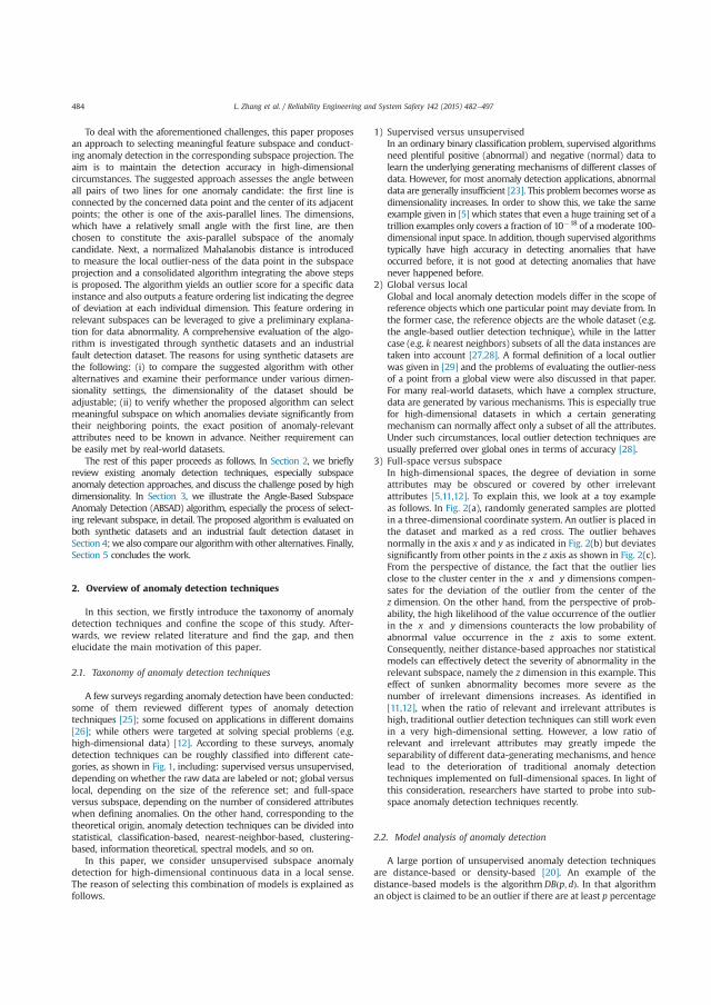
To deal with the aforementioned challenges, this paper proposesan approach to selecting meaningful feature subspace and conduct-ing anomaly detection in the corresponding subspace projection. Theaim is to maintain the detection accuracy in high-dimensionalcircumstances. The suggested approach assesses the angle betweenall pairs of two lines for one anomaly candidate: the first line isconnected by the concerned data point and the center of its adjacentpoints; the other is one of the axis-parallel lines. The dimensions,which have a relatively small angle with the first line, are thenchosen to constitute the axis-parallel subspace of the anomalycandidate. Next, a normalized Mahalanobis distance is introducedto measure the local outlier-ness of the data point in the subspaceprojection and a consolidated algorithm integrating the above stepsis proposed. The algorithm yields an outlier score for a specific datainstance and also outputs a feature ordering list indicating the degreeof deviation at each individual dimension. This feature ordering inrelevant subspaces can be leveraged to give a preliminary explana-tion for data abnormality. A comprehensive evaluation of the algo-rithm is investigated through synthetic datasets and an industrialfault detection dataset. The reasons for using synthetic datasets arethe following: (i) to compare the suggested algorithm with otheralternatives and examine their performance under various dimen-sionality settings, the dimensionality of the dataset should beadjustable; (ii) to verify whether the proposed algorithm can selectmeaningful subspace on which anomalies deviate significantly fromtheir neighboring points, the exact position of anomaly-relevantattributes need to be known in advance. Neither requirement canbe easily met by real-world datasets.
The rest of this paper proceeds as follows. In Section 2, we brieflyreview existing anomaly detection techniques, especially subspaceanomaly detection approaches, and discuss the challenge posed by highdimensionality. In Section 3, we illustrate the Angle-Based SubspaceAnomaly Detection (ABSAD) algorithm, especially the process of select-ing relevant subspace, in detail. The proposed algorithm is evaluated onboth synthetic datasets and an industrial fault detection dataset inSection 4; we also compare our algorithmwith other alternatives. Finally,Section 5 concludes the work.
2. Overview of anomaly detection techniques
In this section, we firstly introduce the taxonomy of anomalydetection techniques and confine the scope of this study. After-wards, we review related literature and find the gap, and thenelucidate the main motivation of this paper.
2.1. Taxonomy of anomaly detection techniques
A few surveys regarding anomaly detection have been conducted:some of them reviewed different types of anomaly detectiontechniques [25]; some focused on applications in different domains[26]; while others were targeted at solving special problems (e.g.high-dimensional data) [12]. According to these surveys, anomalydetection techniques can be roughly classified into different cate-gories, as shown in Fig. 1, including: supervised versus unsupervised,depending on whether the raw data are labeled or not; global versuslocal, depending on the size of the reference set; and full-spaceversus subspace, depending on the number of considered attributeswhen defining anomalies. On the other hand, corresponding to thetheoretical origin, anomaly detection techniques can be divided intostatistical, classification-based, nearest-neighbor-based, clustering-based, information theoretical, spectral models, and so on.
In this paper, we consider unsupervised subspace anomalydetection for high-dimensional continuous data in a local sense.The reason of selecting this combination of models is explained asfollows.
1) Supervised versus unsupervisedIn an ordinary binary classification problem, supervised algorithmsneed plentiful positive (abnormal) and negative (normal) data tolearn the underlying generating mechanisms of different classes ofdata. However, for most anomaly detection applications, abnormaldata are generally insufficient [23]. This problem becomes worse asdimensionality increases. In order to show this, we take the sameexample given in [5] which states that even a huge training set of atrillion examples only covers a fraction of 10�18 of a moderate 100-dimensional input space. In addition, though supervised algorithmstypically have high accuracy in detecting anomalies that haveoccurred before, it is not good at detecting anomalies that havenever happened before.
2) Global versus localGlobal and local anomaly detection models differ in the scope ofreference objects which one particular point may deviate from. Inthe former case, the reference objects are the whole dataset (e.g.the angle-based outlier detection technique), while in the lattercase (e.g. k nearest neighbors) subsets of all the data instances aretaken into account [27,28]. A formal definition of a local outlierwas given in [29] and the problems of evaluating the outlier-nessof a point from a global view were also discussed in that paper.For many real-world datasets, which have a complex structure,data are generated by various mechanisms. This is especially truefor high-dimensional datasets in which a certain generatingmechanism can normally affect only a subset of all the attributes.Under such circumstances, local outlier detection techniques areusually preferred over global ones in terms of accuracy [28].
3) Full-space versus subspaceIn high-dimensional spaces, the degree of deviation in someattributes may be obscured or covered by other irrelevantattributes [5,11,12]. To explain this, we look at a toy exampleas follows. In Fig. 2(a), randomly generated samples are plottedin a three-dimensional coordinate system. An outlier is placed inthe dataset and marked as a red cross. The outlier behavesnormally in the axis x and y as indicated in Fig. 2(b) but deviatessignificantly from other points in the z axis as shown in Fig. 2(c).From the perspective of distance, the fact that the outlier liesclose to the cluster center in the x and y dimensions compen-sates for the deviation of the outlier from the center of thez dimension. On the other hand, from the perspective of prob-ability, the high likelihood of the value occurrence of the outlierin the x and y dimensions counteracts the low probability ofabnormal value occurrence in the z axis to some extent.Consequently, neither distance-based approaches nor statisticalmodels can effectively detect the severity of abnormality in therelevant subspace, namely the z dimension in this example. Thiseffect of sunken abnormality becomes more severe as thenumber of irrelevant dimensions increases. As identified in[11,12], when the ratio of relevant and irrelevant attributes ishigh, traditional outlier detection techniques can still work evenin a very high-dimensional setting. However, a low ratio ofrelevant and irrelevant attributes may greatly impede theseparability of different data-generating mechanisms, and hencelead to the deterioration of traditional anomaly detectiontechniques implemented on full-dimensional spaces. In light ofthis consideration, researchers have started to probe into sub-space anomaly detection techniques recently.
2.2. Model analysis of anomaly detection
A large portion of unsupervised anomaly detection techniquesare distance-based or density-based [20]. An example of thedistance-based models is the algorithm DBðp; dÞ. In that algorithman object is claimed to be an outlier if there are at least p percentage
L. Zhang et al. / Reliability Engineering and System Safety 142 (2015) 482–497484
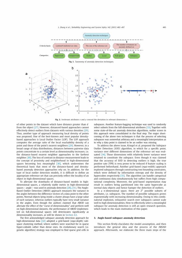
of other points in the dataset which have distance greater than dfrom the object [27]. However, distanced-based approaches cannoteffectively detect outliers from datasets with various densities [29].Thus, another type of approach measuring local density of pointswas proposed. One of the best-known and most popular density-based approaches is Local Outlier Factor (LOF). The LOF approachcomputes the average ratio of the local reachability density of apoint and those of the point's nearest neighbors [29]. However, in abroad range of data distributions, distances between pairwise datapoints concentrate to a certain level as dimensionality increases, i.e.the distance-based nearest neighbor approaches to the farthestneighbor [30]. The loss of contrast in distance measurement leads tothe concept of proximity and neighborhood in high-dimensionalspaces becoming less meaningful [30], which undermines thetheoretical basis that most of the distance-based and density-based anomaly detection approaches rely on. In addition, for thetype of local outlier detection models, it is difficult to define anappropriate reference set that can precisely reflect the locality of anobject in high-dimensional spaces.
To alleviate the drawbacks of distance-based models in high-dimensional spaces, a relatively stable metric in high-dimensionalspaces – angle –was used in anomaly detection [28], [31]. The Angle-Based Outlier Detection (ABOD) approach measures the variance inthe angles between the difference vectors of a data point to the otherpoints. Normal objects lying inside a cluster always have a large valueof such variance, whereas outliers typically have very small variancein the angles. Even though the authors claimed that ABOD canalleviate the effect of the “curse of dimensionality” and perform wellon high-dimensional datasets, the performance of ABOD implemen-ted on full-dimensional spaces still deteriorates significantly asdimensionality increases, as will be shown in Section 4.1.
The first acknowledged subspace anomaly detection approach forhigh-dimensional data [32] adopted a grid-based (equi-depth) sub-space clustering method, where outliers were searched for in sparsehyper-cuboids rather than dense ones. An evolutionary search (i.e.genetic algorithm) strategy was employed to find sparse grid cells in
subspaces. Another feature-bagging technique was used to randomlyselect subsets from the full-dimensional attributes [33]. Together withsome state-of-the-art anomaly detection algorithms, outlier scores inthis approach were consolidated in the final step. The major short-coming of the above two techniques is that the process of selectingsubspaces was somewhat arbitrary and a meaningful interpretation asto why a data point is claimed to be an outlier was missing.
To address the above issue, Kriegel et al. proposed the SubspaceOutlier Detection (SOD) algorithm, in which for a specific point,variance over different dimensions of the reference set was eval-uated [34]. Those dimensions with relatively lower variance wereretained to constitute the subspace. Even though it was claimedthat the accuracy of SOD in detecting outliers is high, the truepositive rate (TPR) is very prone to be reduced if feature scaling isperformed beforehand. Another grid-based (equi-width) approachexplored subspaces through constructing two bounding constraints,which were defined by information entropy and the density ofhypercubes respectively [35]. The algorithm can handle categoricaland continuous data simultaneously but suffers from high compu-tational complexity. Moreover, the grid-based segmentation mayresult in outliers being partitioned into the same hypercube asnormal data objects and hence hamper the detection of outliers.
In a n-dimensional space, there are 2n possible subsets ofattributes, i.e. subspaces. The number of possible subspaces growsexponentially with increasing dimensionality. Owing to this combi-natorial explosion, exhaustive search over subspaces cannot scalewell to high dimensionalities. How to effectively select a meaningfulsubspace for anomaly detection is still an open research question,which leads to the main motivation of this paper.
3. Angle-based subspace anomaly detection
This section firstly elucidates the model assumption, and thenintroduces the general idea and the process of the ABSADapproach. Afterwards, we elaborate the three main steps of the
Criteria basis:
Categories:
Anomaly detection techniques
The number of features an anomaly defined on
Supervised Unsupervised
The size of the reference set
Global Local Full-space Subspace
Labeled/Unlabeled raw data
Fig. 1. Taxonomy of anomaly detection techniques.
Fig. 2. Irrelevant attributes x and y conceal the deviation in relevant dimension z.
L. Zhang et al. / Reliability Engineering and System Safety 142 (2015) 482–497 485
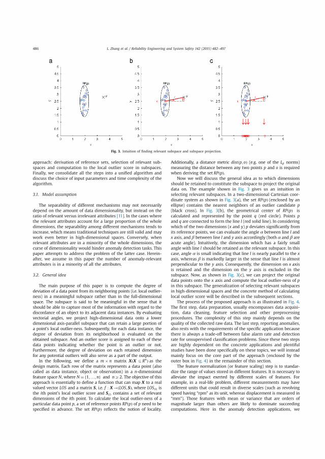
approach: derivation of reference sets, selection of relevant sub-spaces and computation to the local outlier score in subspaces.Finally, we consolidate all the steps into a unified algorithm anddiscuss the choice of input parameters and time complexity of thealgorithm.
3.1. Model assumption
The separability of different mechanisms may not necessarilydepend on the amount of data dimensionality, but instead on theratio of relevant versus irrelevant attributes [11]. In the cases wherethe relevant attributes account for a large proportion of the wholedimensions, the separability among different mechanisms tends toincrease, which means traditional techniques are still valid and maywork even better in high-dimensional spaces. Conversely, whenrelevant attributes are in a minority of the whole dimensions, thecurse of dimensionality would hinder anomaly detection tasks. Thispaper attempts to address the problem of the latter case. Herein-after, we assume in this paper the number of anomaly-relevantattributes is in a minority of all the attributes.
3.2. General idea
The main purpose of this paper is to compute the degree ofdeviation of a data point from its neighboring points (i.e. local outlier-ness) in a meaningful subspace rather than in the full-dimensionalspace. The subspace is said to be meaningful in the sense that itshould be able to capture most of the information with regard to thediscordance of an object to its adjacent data instances. By evaluatingvectorial angles, we project high-dimensional data onto a lowerdimensional axis-parallel subspace that can retain a large portion ofa point's local outlier-ness. Subsequently, for each data instance, thedegree of deviation from its neighborhood is evaluated on theobtained subspace. And an outlier score is assigned to each of thesedata points indicating whether the point is an outlier or not.Furthermore, the degree of deviation on each retained dimensionfor any potential outliers will also serve as a part of the output.
In the following, we define a m� n matrix XðX DRnÞ as thedesign matrix. Each row of the matrix represents a data point (alsocalled as data instance, object or observation) in a n-dimensionalfeature space N, where N¼ 1;…;nf g and nZ2. The objective of thisapproach is essentially to define a function that can map X to a realvalued vector LOS and a matrix S, i.e. f : X-ðLOS; SÞ, where LOSðiÞ isthe ith point's local outlier score and SðiÞ contains a set of relevantdimensions of the ith point. To calculate the local outlier-ness of aparticular data point p, a set of reference points RPðpÞ of p need to bespecified in advance. The set RPðpÞ reflects the notion of locality.
Additionally, a distance metric distðp; oÞ (e.g. one of the Lp norms)measuring the distance between any two points p and o is requiredwhen deriving the set RPðpÞ.
Now we will discuss the general idea as to which dimensionsshould be retained to constitute the subspace to project the originaldata on. The example shown in Fig. 3 gives us an intuition inselecting relevant subspaces. In a two-dimensional Cartesian coor-dinate system as shown in Fig. 3(a), the set RP pð Þ (enclosed by anellipse) contains the nearest neighbors of an outlier candidate p(black cross). In Fig. 3(b), the geometrical center of RP pð Þ iscalculated and represented by the point q (red circle). Points pand q are connected to form the line l (red solid line). In consideringwhich of the two dimensions (x and y) p deviates significantly fromits reference points, we can evaluate the angle α between line l andx axis, and β between line l and y axis accordingly (both α and β areacute angle). Intuitively, the dimension which has a fairly smallangle with line l should be retained as the relevant subspace. In thiscase, angle α is small indicating that line l is nearly parallel to the xaxis, whereas β is markedly larger in the sense that line l is almostperpendicular to the y axis. Consequently, the dimension on x axisis retained and the dimension on the y axis is excluded in thesubspace. Now, as shown in Fig. 3(c), we can project the originaldata points onto the x axis and compute the local outlier-ness of pin this subspace. The generalization of selecting relevant subspacesin high-dimensional spaces and the concrete method of calculatinglocal outlier score will be described in the subsequent sections.
The process of the proposed approach is as illustrated in Fig. 4.The first step, data preparation, usually encompasses data acquisi-tion, data cleaning, feature selection and other preprocessingprocedures. The complexity of this step mainly depends on thequality of the collected raw data. The last step, reporting anomalies,also rests with the requirements of the specific application becausethere is always a trade-off between false alarm rate and detectionrate for unsupervised classification problems. Since these two stepsare highly dependent on the concrete applications and plentifulstudies have been done specifically on these topics, we will insteadmainly focus on the core part of the approach (enclosed by theouter box in Fig. 4) in the remainder of this section.
The feature normalization (or feature scaling) step is to standar-dize the range of values stored in different features. It is necessary toalleviate the impact exerted by different scales of features. Forexample, in a real-life problem, different measurements may havedifferent units that could result in diverse scales (such as revolvingspeed having “rpm” as its unit, whereas displacement is measured in“mm”). Those features with mean or variance that are orders ofmagnitude larger than others are likely to dominate succeedingcomputations. Here in the anomaly detection applications, we
Fig. 3. Intuition of finding relevant subspace and subspace projection.
L. Zhang et al. / Reliability Engineering and System Safety 142 (2015) 482–497486
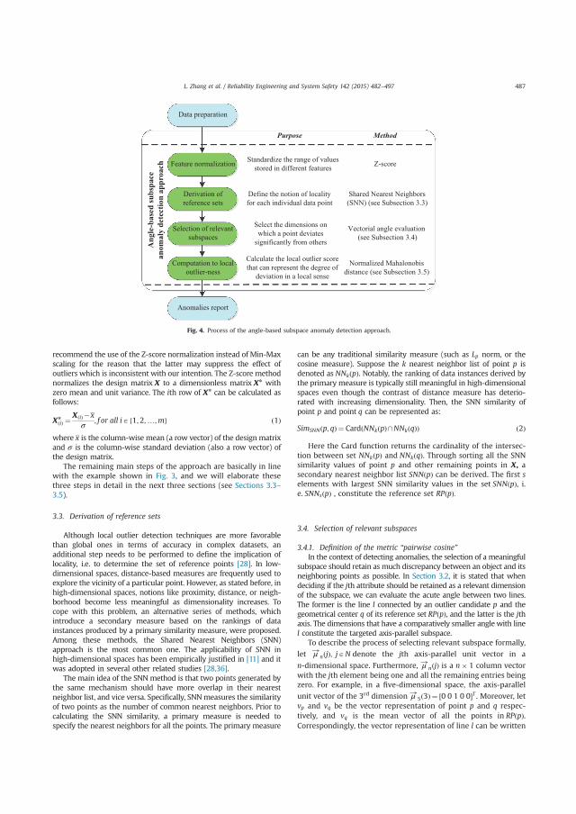
recommend the use of the Z-score normalization instead of Min-Maxscaling for the reason that the latter may suppress the effect ofoutliers which is inconsistent with our intention. The Z-score methodnormalizes the design matrix X to a dimensionless matrix Xn withzero mean and unit variance. The ith row of Xn can be calculated asfollows:
Xn
ðiÞ ¼X ið Þ �xσ
; f or all iA 1;2;…;mf g ð1Þ
where x is the column-wise mean (a row vector) of the design matrixand σ is the column-wise standard deviation (also a row vector) ofthe design matrix.
The remaining main steps of the approach are basically in linewith the example shown in Fig. 3, and we will elaborate thesethree steps in detail in the next three sections (see Sections 3.3–3.5).
3.3. Derivation of reference sets
Although local outlier detection techniques are more favorablethan global ones in terms of accuracy in complex datasets, anadditional step needs to be performed to define the implication oflocality, i.e. to determine the set of reference points [28]. In low-dimensional spaces, distance-based measures are frequently used toexplore the vicinity of a particular point. However, as stated before, inhigh-dimensional spaces, notions like proximity, distance, or neigh-borhood become less meaningful as dimensionality increases. Tocope with this problem, an alternative series of methods, whichintroduce a secondary measure based on the rankings of datainstances produced by a primary similarity measure, were proposed.Among these methods, the Shared Nearest Neighbors (SNN)approach is the most common one. The applicability of SNN inhigh-dimensional spaces has been empirically justified in [11] and itwas adopted in several other related studies [28,36].
The main idea of the SNN method is that two points generated bythe same mechanism should have more overlap in their nearestneighbor list, and vice versa. Specifically, SNNmeasures the similarityof two points as the number of common nearest neighbors. Prior tocalculating the SNN similarity, a primary measure is needed tospecify the nearest neighbors for all the points. The primary measure
can be any traditional similarity measure (such as Lp norm, or thecosine measure). Suppose the k nearest neighbor list of point p isdenoted as NNk pð Þ. Notably, the ranking of data instances derived bythe primary measure is typically still meaningful in high-dimensionalspaces even though the contrast of distance measure has deterio-rated with increasing dimensionality. Then, the SNN similarity ofpoint p and point q can be represented as:
SimSNN p; qð Þ ¼ CardðNNkðpÞ\NNkðqÞÞ ð2Þ
Here the Card function returns the cardinality of the intersec-tion between set NNkðpÞ and NNkðqÞ. Through sorting all the SNNsimilarity values of point p and other remaining points in X, asecondary nearest neighbor list SNNðpÞ can be derived. The first selements with largest SNN similarity values in the set SNNðpÞ, i.e. SNNsðpÞ , constitute the reference set RP pð Þ:
3.4. Selection of relevant subspaces
3.4.1. Definition of the metric “pairwise cosine”In the context of detecting anomalies, the selection of a meaningful
subspace should retain as much discrepancy between an object and itsneighboring points as possible. In Section 3.2, it is stated that whendeciding if the jth attribute should be retained as a relevant dimensionof the subspace, we can evaluate the acute angle between two lines.The former is the line l connected by an outlier candidate p and thegeometrical center q of its reference set RPðpÞ, and the latter is the jthaxis. The dimensions that have a comparatively smaller angle with linel constitute the targeted axis-parallel subspace.
To describe the process of selecting relevant subspace formally,
let μ!n jð Þ; jAN denote the jth axis-parallel unit vector in a
n-dimensional space. Furthermore, μ!nðjÞ is a n� 1 column vectorwith the jth element being one and all the remaining entries beingzero. For example, in a five-dimensional space, the axis-parallel
unit vector of the 3rd dimension μ!5ð3Þ ¼ ½0 0 1 0 0�T . Moreover, letvp and vq be the vector representation of point p and q respec-tively, and vq is the mean vector of all the points in RPðpÞ.Correspondingly, the vector representation of line l can be written
Angle-basedsubspace
anomalydetectionapproach
Define the notion of locality for each individual data point
Standardize the range of values stored in different features
Select the dimensions on which a point deviates
significantly from others
Calculate the local outlier score that can represent the degree of
deviation in a local sense
Purpose Method
Z-score
Shared Nearest Neighbors (SNN) (see Subsection 3.3)
Vectorial angle evaluation(see Subsection 3.4)
Normalized Mahalonobis distance (see Subsection 3.5)
Data preparation
Anomalies report
Feature normalization
Derivation of reference sets
Selection of relevant subspaces
Computation to local outlier-ness
Fig. 4. Process of the angle-based subspace anomaly detection approach.
L. Zhang et al. / Reliability Engineering and System Safety 142 (2015) 482–497 487
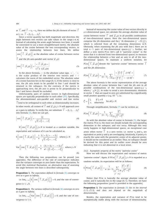
as l!
, and l!¼ vp�vq. Here we define the jth element of vector l
!
as lj, i.e. l!¼ ½l1; l2;…; ln�T .
Since a vector quantity has both magnitude and direction, theangle between two vectors can take values in the range –π;π½ �.Instead of calculating the acute angle between two lines, it wouldbe convenient to use a more straightforward metric, the absolutevalue of the cosine between the two corresponding vectors, toassess the relationship between two lines. We define
cos l!
; μ!nðjÞ� �����
���� as the absolute value of cosine between vector
l!
and the jth axis-parallel unit vector μ!nðjÞ:
cos l!
; μ!n jð Þ� �����
����¼ o l!
; μ!n jð Þ4��� ���∥ l!
∥U∥ μ!n jð Þ∥ð3Þ
In the above formula, Uj j is the absolute value sign, o U ; U4is the scalar product of the interior two vectors and J U Jcalculates the norm of the embedded vector. The absolute valueof a cosine function lies in the range [0, 1]. If the metric is close toone, the jth axis tends to be parallel to line l and should beretained in the subspace. On the contrary, if the metric isapproaching zero, the jth axis is prone to be perpendicular toline l and hence should be excluded.
Unfortunately, pairs of random vectors in high-dimensionalspaces are typically perpendicular to each other [37]. Specifically,the aforementioned axis-parallel unit vectors and line vector
l!
tend to be orthogonal to each other as dimensionality increases.
In other words, all cosines of l!
and μ!n jð Þ; jAN will approach zero
as n goes to infinity. To verify this, we substitute l! ¼ ½l1; l2;…; ln�T
into formula (3), then we can get,
cos l!
; μ!n jð Þ� �����
����¼ lj�� ��ffiffiffiffiffiffiffiffiffiffiffiffiffiffiffiffiffiffiffiffiffiffiffiffiffiffiffiffiffiffi
l21þ l22þ…þ l2n
q ð4Þ
If cos l!
; μ!nðjÞ� �����
����; jAN is treated as a random variable, the
expectation and variance of it can be calculated as,
E cos l!
; μ!n jð Þ� �����
�����
¼ 1nUl1�� ��þ l2
�� ��þ…þ ln�� ��ffiffiffiffiffiffiffiffiffiffiffiffiffiffiffiffiffiffiffiffiffiffiffiffiffiffiffiffiffiffi
l21þ l22þ…þ l2n
q ; where jAN ð5Þ
Var cos l!
; μ!n jð Þ� �����
�����
¼ 1n� l1�� ��þ l2
�� ��þ…þ ln�� �� �2
n2 U l21þ l22þ…þ l2n� ; where jAN
ð6Þ
Then the following two propositions can be proved (seeappendix). The difference of the rate of convergence indicatesthat the variance converges to zero faster than the expectation. Toavoid this statistical fluctuation, an alternative way of assessingthe angle between two lines is described subsequently.
Proposition 1. The expectation defined in formula (5) converges tozero as n goes to infinity,
i.e. limn-1 E cos l!
; μ!n jð Þ� �����
����� � �
¼ 0, and the rate of conver-
gence is 1=ffiffiffin
p.
Proposition 2. The variance defined in formula (6) converges to zeroas n goes to infinity,
i.e. limn-1 Var cos l!
; μ!n jð Þ� �����
����� � �
¼ 0, and the rate of con-
vergence is 1=n.
Instead of measuring the cosine value of two vectors directly ina n-dimensional space, we calculate the average absolute value of
cosine between vector l!
and μ!n jð Þ in all possible combinationsof two-dimensional spaces. Here the two-dimensional spacescomprise the jth dimension and the j� th dimension (j� AN\ j
� �),
which is selected from all the remaining dimensions in N.Obviously, when examining the jth axis with line l, there are intotal n�1 pairs of two-dimensional spaces j; j�ð Þ. Further, wedefine a new metric PCos (let's call it “pairwise cosine” in thesense that it is derived from two-dimensional spaces) to measurethe relationship between a line and an axis in all of the two-dimensional spaces. To maintain a uniform notation, let
PCos l!
; μ!n jð Þ� �
denote the “pairwise cosine” between vector l!
and the jth dimension:
PCos l!
; μ!n jð Þ� �
¼ 1n�1ð Þ
Xj� AN\ jf g
o l#j l#j�h iT
; 1 0½ �T 4����
����J l#j l#j�h iT
J U J 1 0½ �T Jð7Þ
The above formula is the vector representation of the averageabsolute value of cosine between line l and the jth axis in allpossible combinations of the two-dimensional spaces j; j�ð Þ,where j� AN\ j
� �. In order to avoid a zero denominator, elements
in vector l!
that are equal to zero are substituted by a significantlysmall positive quantity ε (e.g. 10�5), i.e.
l#j ¼lj; if lja0ε; otherwise
(for all jAN
Through simplification, formula (7) can be written as:
PCos l!
; μ!n jð Þ� �
¼ 1n�1ð Þ
Xj� AN\ jf g
l#j��� ���ffiffiffiffiffiffiffiffiffiffiffiffiffiffiffiffiffil#2j þ l#2j�
q ð8Þ
As with the absolute value of cosine in formula (3), the largerthe metric PCos is, the more we should include the correspondingdimension in the subspace, and vice versa. Although this veryrarely happens in high-dimensional spaces, an exceptional case
arises when vector l!
is a zero vector, i.e. vector vp and vq areequivalent or point p and q are overlapping. Intuitively, if point p isexactly the same with the geometric center of its adjacent points,it should not be considered as an outlier. Thus, no subspace shouldbe derived for this point and its outlier score should be zeroindicating that it is not abnormal in a local sense.
3.4.2. Asymptotic property of the metric “pairwise cosine”Now we will discuss the expectation and variance of metric
“pairwise cosine”. Again, if PCos l!
; μ!n jð Þ� �
; jAN is regarded as a
random variable, its expectation will be as follows:
E PCos l!
; μ!n jð Þ� ��
¼ 1nUðn�1Þ
Xj; j� AN
j� a j
l#j��� ���þ l#j�
��� ���ffiffiffiffiffiffiffiffiffiffiffiffiffiffiffiffiffil#2j þ l#2j�
q ð9Þ
Notice that PCos is basically the average absolute value ofcosine, and it naturally lies in the range [0, 1]. Therefore, we havethe following proposition (proof is provided in the appendix).
Proposition 3. The expectation in formula (9) lies in the intervalð1=2;
ffiffiffi2
p=2� and does not depend on the magnitude of
dimensionality.
Besides, the expectation and variance of PCos tend to beasymptotically stable along with the increase of dimensionality.
L. Zhang et al. / Reliability Engineering and System Safety 142 (2015) 482–497488
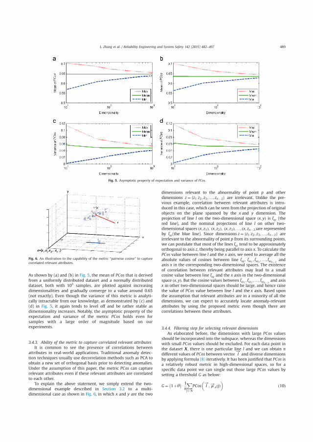
As shown by (a) and (b) in Fig. 5, the mean of PCos that is derivedfrom a uniformly distributed dataset and a normally distributeddataset, both with 105 samples, are plotted against increasingdimensionalities and gradually converge to a value around 0.65(not exactly). Even though the variance of this metric is analyti-cally intractable from our knowledge, as demonstrated by (c) and(d) in Fig. 5, it again tends to level off and be rather stable asdimensionality increases. Notably, the asymptotic property of theexpectation and variance of the metric PCos holds even forsamples with a large order of magnitude based on ourexperiments.
3.4.3. Ability of the metric to capture correlated relevant attributesIt is common to see the presence of correlations between
attributes in real-world applications. Traditional anomaly detec-tion techniques usually use decorrelation methods such as PCA toobtain a new set of orthogonal basis prior to detecting anomalies.Under the assumption of this paper, the metric PCos can capturerelevant attributes even if these relevant attributes are correlatedto each other.
To explain the above statement, we simply extend the two-dimensional example described in Section 3.2 to a multi-dimensional case as shown in Fig. 6, in which x and y are the two
dimensions relevant to the abnormality of point p and otherdimensions z¼ z1 z2; z3;…; zn�2f g are irrelevant. Unlike the pre-vious example, correlation between relevant attributes is intro-duced in this case, which can be seen from the projection of originalobjects on the plane spanned by the x and y dimension. Theprojection of line l on the two-dimensional space ðx; yÞ is l0xy (thered line), and the nominal projections of line l on other two-dimensional spaces x; z1ð Þ; x; z2ð Þ; x; z3ð Þ;…; ðx; zn�2Þare representedby l0xz(the blue line). Since dimensions z¼ z1 z2; z3;…; zn�2f g areirrelevant to the abnormality of point p from its surrounding points,we can postulate that most of the lines l0xz tend to be approximatelyorthogonal to axis z, thereby being parallel to axis x. To calculate thePCos value between line l and the x axis, we need to average all theabsolute values of cosines between line l0xy; l
0xz1 ; l
0xz2 ;…; l0xzn� 2
andaxis x in the corresponding two-dimensional spaces. The existenceof correlation between relevant attributes may lead to a smallcosine value between line l0xy and the x axis in the two-dimensionalspace ðx; yÞ. But the cosine values between l0xz1 ; l
0xz2 ;…; l0xzn� 2
and axisx in other two-dimensional spaces should be large, and hence raisethe value of PCos value between line l and the x axis. Based uponthe assumption that relevant attributes are in a minority of all thedimensions, we can expect to accurately locate anomaly-relevantattributes by using the proposed metric even though there arecorrelations between these attributes.
3.4.4. Filtering step for selecting relevant dimensionsAs elaborated before, the dimensions with large PCos values
should be incorporated into the subspace, whereas the dimensionswith small PCos values should be excluded. For each data point inthe dataset X, there is one particular line l and we can obtain ndifferent values of PCos between vector l
!and diverse dimensions
by applying formula (8) iteratively. It has been justified that PCos isa relatively robust metric in high-dimensional spaces, so for aspecific data point we can single out those large PCos values bysetting a threshold G as below:
G¼ 1þθ �
U1n
XjAN
PCos l!
; μ!n jð Þ� �
ð10Þ
Fig. 5. Asymptotic property of expectation and variance of PCos.
Fig. 6. An illustration to the capability of the metric “pairwise cosine” to capturecorrelated relevant attributes.
L. Zhang et al. / Reliability Engineering and System Safety 142 (2015) 482–497 489

Here, θ is an input parameter lying in ½0; 1Þ, and the right part ofthe multiplier in formula (10) is the average PCos over all thedimensions. Those dimensions with a PCos value greater than G areretained to constitute the relevant subspace for a specific data point.Further, we can save the obtained subspace index into S, which is am� n matrix. Concretely, the ith row of the matrix SðiÞ stores therelevant subspace of the corresponding ith data point, and the jthcolumn defines whether the jth attribute should be retained. Wesuppose SðiÞ jð Þ locates to the cell of the ith row and the jth column. Ifwe are considering the ith data point, and the jth attribute is singledout to be retained, then SðiÞ jð Þ ¼ 1, otherwise SðiÞ jð Þ ¼ 0.
3.5. Computation to local outlier-ness in subspaces
After going through the process of selecting relevant subspace foreach data point, we might find that some of the points do not haveany relevant attributes retained as a part of the subspace. In otherwords, when the ith point conforms to this situation, SðiÞ jð Þ equals tozero for all jAN. This circumstance shows that the ith point does notsignificantly deviate from its neighbors in any subsets of all thedimensions. To explain this, we can imagine that if a point doesdeviate from its neighbors in a subset of all the attributes, thereshould be some extreme values in the “pairwise cosine” that wouldbe captured by the filtering step. Thus, for those points with nosubspace to project on, we simply set the outlier score to zero.
In the following, we describe how to measure the local outlier-less of a data point in its subspace. Normally, some state-of-the-arttechniques (e.g. distance-based, density-based, statistical models)which can effectively and efficiently detect anomalies in low-dimensional spaces are employed to calculate the overall outlier-ness at this stage. For example, in the SOD algorithm [34], Euclideandistance is utilized to calculate the local outlier-ness of a point in thesubspace projection. Generally, these methods are also applicable inour algorithm and can performwell if the outlier score is normalizedin a good manner. However, a single outlier score can neither revealthe degree of deviation in each individual dimension for an outliernor provide a rank to the degree of deviation in these dimensions.Hereinafter, we compute the local outlier-ness of an outlier candidatein two steps: measure the overall local outlier score; calculate itsdegree of deviation on each individual dimension of the obtainedsubspace. By doing so, not only a comprehensive outlier score can bederived but also a preliminary interpretation as to why a point isclassified as an outlier can be provided.
3.5.1. Overall local outlier scoreDue to the possible existence of correlation between the retained
dimensions, we introduce a normalized Mahalanobis distance tomeasure the overall local outlier score in the subspace for a specificdata point. Firstly, let Xn0
ið Þ be the vector representation (a row vector)of the ith normalized point's projection on the retained subspace,and RPðiÞ0 denotes the set of the projected reference points of theoriginal reference points RPðiÞ on the retained subspace. Secondly,the mean vector of the reference point's projection is denoted asRPðiÞ0 (also a row vector), and the inverse of the covariance matrix ofthe projected reference points RPðiÞ0 is Σ�1
RPðiÞ0 . Further, let dðiÞ denotethe number of retained dimensions for the ith data point. Then thelocal outlier score for the ith point LOS ið Þ is defined as follows:
LOS ið Þ ¼ 1dðiÞU
ffiffiffiffiffiffiffiffiffiffiffiffiffiffiffiffiffiffiffiffiffiffiffiffiffiffiffiffiffiffiffiffiffiffiffiffiffiffiffiffiffiffiffiffiffiffiffiffiffiffiffiffiffiffiffiffiffiffiffiffiffiffiffiffiffiffiffiffiðXn0
ið Þ �RPðiÞ0 ÞΣ�1RPðiÞ0 ðXn0
ið Þ �RPðiÞ0 ÞTq
ð11Þ
In formula (11), the right side of the multiplier is essentially theMahalanobis distance from the normalized point i to its referencepoints in the subspace projection. Essentially, the local outlier scorefor the ith point LOS ið Þ is the Mahalanobis distance in the retainedsubspace normalized by the number of retained dimensions.
Notably, for the covariance matrix of the projected referencepoints ΣRPðiÞ0 to be invertible, the covariance matrix should be non-singular. The non-singularity of the covariance matrix relies on thefollowing three prerequisites: (i) in the data preparation step, featureselection has eliminated redundant attributes and the retaineddimensions in the subspace are not highly correlated; (ii) weassumed that the anomaly-relevant attributes are in a minority ofall the dimensions in Section 3.1 and the process of selecting relevantsubspaces described in Section 3.4.4 should filter out large amount ofanomaly-irrelevant attributes, and hence the number of retaineddimensions is small; (iii) the choice of the number of reference pointss (as will be discussed in Section 3.6.2) should be set large enough.The above three conditions can basically suffice for the non-singularity of the covariance matrix.
3.5.2. Degree of deviation on each individual dimensionNow we will discuss the calculation to the degree of deviation
on each individual dimension of the obtained subspace. Intuitively,the overall local outlier score LOSðiÞ can be viewed as the length ofthe line connected by the ith normalized point and its referencepoints in the subspace projection, i.e. the length of the line
Xn0ið Þ �RPðiÞ0 . For the ith point, the degree of deviation on the
retained jth dimension LOSði; jÞ can be measured by the length ofprojection from the above line onto the jth dimension in the
subspace. To adhere to a consistent notation, let μ!d ið Þ jð Þ denote thejth axis-parallel unit vector in the ith point's retained subspace
and γij be the angle between the line Xn0ið Þ �RPðiÞ0 and the jth axis of
the subspace. Then LOS i; jð Þ can be calculated as below:
LOS i; jð Þ ¼ cos ðγijÞ��� ���ULOS ið Þ ¼
Xn 0ið Þ �RP ið Þ0 ; μ!d ið Þ jð Þ
D E��� ���JXn0
ið Þ �RP ið Þ0 J U J μ!d ið Þ jð ÞJULOSðiÞ
ð12ÞThe expanded form of cos ðγijÞ
��� ��� in formula (12) is similar toformula (3) and the metric LOSði; jÞ is essentially to measure thelength of the projection from one vector to another vector in thesubspace. Due to the triangle inequality, the obtained local outlierscore on each individual dimension is not comparable with theoverall local outlier score. Furthermore, the single-dimensional localoutlier score cannot be compared across different points. But for aparticular data point, the difference of these single-dimensional localoutlier scores of one point can reflect the magnitude of influence tothe overall local outlier-ness contributed by different dimensions.
At this stage, we are able to discern anomaly-relevant attri-butes from matrix S for a particular point. In the case of severaldimensions being retained, a rank to these dimensions accordingto the single-dimensional local outlier score might facilitatefurther investigation as to the cause of abnormality. Therefore,an update policy applied to matrix S can be implemented aftercalculating all the local outlier scores. The update policy isdescribed as follows:
SðiÞ jð Þ ¼LOSði; jÞ; if SðiÞ jð Þ ¼ 1
0; otherwise
(ð13Þ
Now from matrix S, through ranking those non-zero elementsin a row, one can provide a preliminary explanation as to why adata point is declared to be an anomaly.
3.6. Model integration and discussion
In the preceding sections, we described the main steps of theABSAD algorithm, especially the procedure for finding relevantsubspace by analyzing vectorial angles in high-dimensional spaces.In the following, we streamline the above steps and consolidate
L. Zhang et al. / Reliability Engineering and System Safety 142 (2015) 482–497490
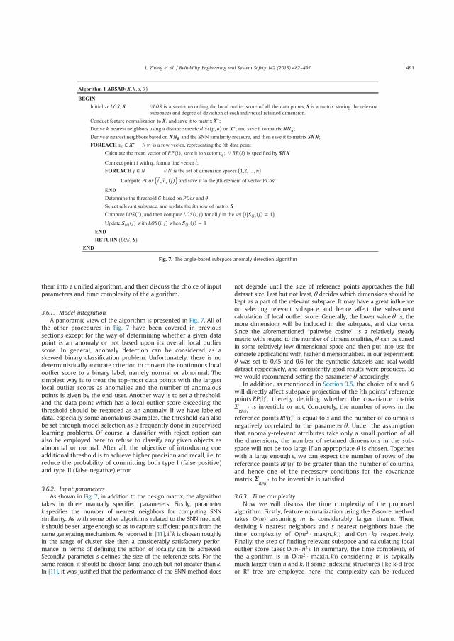
them into a unified algorithm, and then discuss the choice of inputparameters and time complexity of the algorithm.
3.6.1. Model integrationA panoramic view of the algorithm is presented in Fig. 7. All of
the other procedures in Fig. 7 have been covered in previoussections except for the way of determining whether a given datapoint is an anomaly or not based upon its overall local outlierscore. In general, anomaly detection can be considered as askewed binary classification problem. Unfortunately, there is nodeterministically accurate criterion to convert the continuous localoutlier score to a binary label, namely normal or abnormal. Thesimplest way is to treat the top-most data points with the largestlocal outlier scores as anomalies and the number of anomalouspoints is given by the end-user. Another way is to set a threshold,and the data point which has a local outlier score exceeding thethreshold should be regarded as an anomaly. If we have labeleddata, especially some anomalous examples, the threshold can alsobe set through model selection as is frequently done in supervisedlearning problems. Of course, a classifier with reject option canalso be employed here to refuse to classify any given objects asabnormal or normal. After all, the objective of introducing oneadditional threshold is to achieve higher precision and recall, i.e. toreduce the probability of committing both type I (false positive)and type II (false negative) error.
3.6.2. Input parametersAs shown in Fig. 7, in addition to the design matrix, the algorithm
takes in three manually specified parameters. Firstly, parameterk specifies the number of nearest neighbors for computing SNNsimilarity. As with some other algorithms related to the SNN method,k should be set large enough so as to capture sufficient points from thesame generating mechanism. As reported in [11], if k is chosen roughlyin the range of cluster size then a considerably satisfactory perfor-mance in terms of defining the notion of locality can be achieved.Secondly, parameter s defines the size of the reference sets. For thesame reason, it should be chosen large enough but not greater than k.In [11], it was justified that the performance of the SNN method does
not degrade until the size of reference points approaches the fulldataset size. Last but not least, θ decides which dimensions should bekept as a part of the relevant subspace. It may have a great influenceon selecting relevant subspace and hence affect the subsequentcalculation of local outlier score. Generally, the lower value θ is, themore dimensions will be included in the subspace, and vice versa.Since the aforementioned “pairwise cosine” is a relatively steadymetric with regard to the number of dimensionalities, θ can be tunedin some relatively low-dimensional space and then put into use forconcrete applications with higher dimensionalities. In our experiment,θ was set to 0.45 and 0.6 for the synthetic datasets and real-worlddataset respectively, and consistently good results were produced. Sowe would recommend setting the parameter θ accordingly.
In addition, as mentioned in Section 3.5, the choice of s and θwill directly affect subspace projection of the ith points’ referencepoints RPðiÞ0, thereby deciding whether the covariance matrixΣ
RPðiÞ'is invertible or not. Concretely, the number of rows in the
reference points RPðiÞ0 is equal to s and the number of columns isnegatively correlated to the parameter θ. Under the assumptionthat anomaly-relevant attributes take only a small portion of allthe dimensions, the number of retained dimensions in the sub-space will not be too large if an appropriate θ is chosen. Togetherwith a large enough s, we can expect the number of rows of thereference points RPðiÞ0 to be greater than the number of columns,and hence one of the necessary conditions for the covariancematrix Σ
RPðiÞ'to be invertible is satisfied.
3.6.3. Time complexityNow we will discuss the time complexity of the proposed
algorithm. Firstly, feature normalization using the Z-score methodtakes OðmÞ assuming m is considerably larger than n. Then,deriving k nearest neighbors and s nearest neighbors have thetime complexity of Oðm2 U maxðn; kÞÞ and OðmUkÞ respectively.Finally, the step of finding relevant subspace and calculating localoutlier score takes OðmUn2Þ. In summary, the time complexity ofthe algorithm is in Oðm2 U maxðn; kÞÞ considering m is typicallymuch larger than n and k. If some indexing structures like k-d treeor R* tree are employed here, the complexity can be reduced
Fig. 7. The angle-based subspace anomaly detection algorithm
L. Zhang et al. / Reliability Engineering and System Safety 142 (2015) 482–497 491
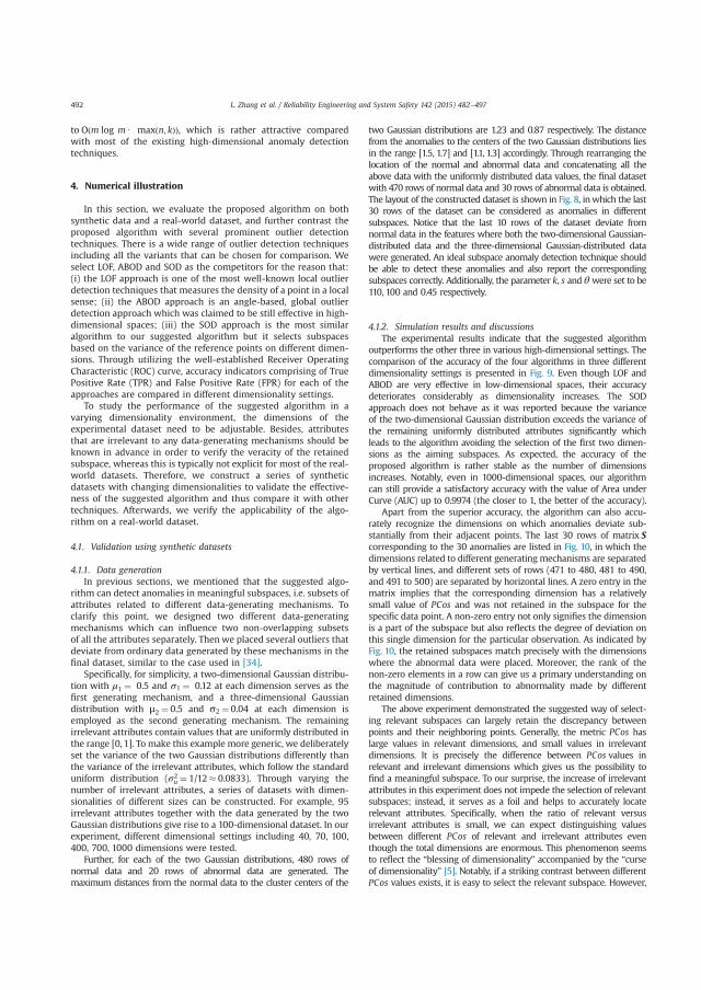
to Oðm log mU maxðn; kÞÞ, which is rather attractive comparedwith most of the existing high-dimensional anomaly detectiontechniques.
4. Numerical illustration
In this section, we evaluate the proposed algorithm on bothsynthetic data and a real-world dataset, and further contrast theproposed algorithm with several prominent outlier detectiontechniques. There is a wide range of outlier detection techniquesincluding all the variants that can be chosen for comparison. Weselect LOF, ABOD and SOD as the competitors for the reason that:(i) the LOF approach is one of the most well-known local outlierdetection techniques that measures the density of a point in a localsense; (ii) the ABOD approach is an angle-based, global outlierdetection approach which was claimed to be still effective in high-dimensional spaces; (iii) the SOD approach is the most similaralgorithm to our suggested algorithm but it selects subspacesbased on the variance of the reference points on different dimen-sions. Through utilizing the well-established Receiver OperatingCharacteristic (ROC) curve, accuracy indicators comprising of TruePositive Rate (TPR) and False Positive Rate (FPR) for each of theapproaches are compared in different dimensionality settings.
To study the performance of the suggested algorithm in avarying dimensionality environment, the dimensions of theexperimental dataset need to be adjustable. Besides, attributesthat are irrelevant to any data-generating mechanisms should beknown in advance in order to verify the veracity of the retainedsubspace, whereas this is typically not explicit for most of the real-world datasets. Therefore, we construct a series of syntheticdatasets with changing dimensionalities to validate the effective-ness of the suggested algorithm and thus compare it with othertechniques. Afterwards, we verify the applicability of the algo-rithm on a real-world dataset.
4.1. Validation using synthetic datasets
4.1.1. Data generationIn previous sections, we mentioned that the suggested algo-
rithm can detect anomalies in meaningful subspaces, i.e. subsets ofattributes related to different data-generating mechanisms. Toclarify this point, we designed two different data-generatingmechanisms which can influence two non-overlapping subsetsof all the attributes separately. Thenwe placed several outliers thatdeviate from ordinary data generated by these mechanisms in thefinal dataset, similar to the case used in [34].
Specifically, for simplicity, a two-dimensional Gaussian distribu-tion with μ1 ¼ 0.5 and σ1 ¼ 0.12 at each dimension serves as thefirst generating mechanism, and a three-dimensional Gaussiandistribution with μ2 ¼ 0.5 and σ2 ¼ 0.04 at each dimension isemployed as the second generating mechanism. The remainingirrelevant attributes contain values that are uniformly distributed inthe range [0, 1]. To make this example more generic, we deliberatelyset the variance of the two Gaussian distributions differently thanthe variance of the irrelevant attributes, which follow the standarduniform distribution (σ2
u ¼ 1/12� 0.0833). Through varying thenumber of irrelevant attributes, a series of datasets with dimen-sionalities of different sizes can be constructed. For example, 95irrelevant attributes together with the data generated by the twoGaussian distributions give rise to a 100-dimensional dataset. In ourexperiment, different dimensional settings including 40, 70, 100,400, 700, 1000 dimensions were tested.
Further, for each of the two Gaussian distributions, 480 rows ofnormal data and 20 rows of abnormal data are generated. Themaximum distances from the normal data to the cluster centers of the
two Gaussian distributions are 1.23 and 0.87 respectively. The distancefrom the anomalies to the centers of the two Gaussian distributions liesin the range [1.5, 1.7] and [1.1, 1.3] accordingly. Through rearranging thelocation of the normal and abnormal data and concatenating all theabove data with the uniformly distributed data values, the final datasetwith 470 rows of normal data and 30 rows of abnormal data is obtained.The layout of the constructed dataset is shown in Fig. 8, inwhich the last30 rows of the dataset can be considered as anomalies in differentsubspaces. Notice that the last 10 rows of the dataset deviate fromnormal data in the features where both the two-dimensional Gaussian-distributed data and the three-dimensional Gaussian-distributed datawere generated. An ideal subspace anomaly detection technique shouldbe able to detect these anomalies and also report the correspondingsubspaces correctly. Additionally, the parameter k, s and θ were set to be110, 100 and 0.45 respectively.
4.1.2. Simulation results and discussionsThe experimental results indicate that the suggested algorithm
outperforms the other three in various high-dimensional settings. Thecomparison of the accuracy of the four algorithms in three differentdimensionality settings is presented in Fig. 9. Even though LOF andABOD are very effective in low-dimensional spaces, their accuracydeteriorates considerably as dimensionality increases. The SODapproach does not behave as it was reported because the varianceof the two-dimensional Gaussian distribution exceeds the variance ofthe remaining uniformly distributed attributes significantly whichleads to the algorithm avoiding the selection of the first two dimen-sions as the aiming subspaces. As expected, the accuracy of theproposed algorithm is rather stable as the number of dimensionsincreases. Notably, even in 1000-dimensional spaces, our algorithmcan still provide a satisfactory accuracy with the value of Area underCurve (AUC) up to 0.9974 (the closer to 1, the better of the accuracy).
Apart from the superior accuracy, the algorithm can also accu-rately recognize the dimensions on which anomalies deviate sub-stantially from their adjacent points. The last 30 rows of matrix Scorresponding to the 30 anomalies are listed in Fig. 10, in which thedimensions related to different generating mechanisms are separatedby vertical lines, and different sets of rows (471 to 480, 481 to 490,and 491 to 500) are separated by horizontal lines. A zero entry in thematrix implies that the corresponding dimension has a relativelysmall value of PCos and was not retained in the subspace for thespecific data point. A non-zero entry not only signifies the dimensionis a part of the subspace but also reflects the degree of deviation onthis single dimension for the particular observation. As indicated byFig. 10, the retained subspaces match precisely with the dimensionswhere the abnormal data were placed. Moreover, the rank of thenon-zero elements in a row can give us a primary understanding onthe magnitude of contribution to abnormality made by differentretained dimensions.
The above experiment demonstrated the suggested way of select-ing relevant subspaces can largely retain the discrepancy betweenpoints and their neighboring points. Generally, the metric PCos haslarge values in relevant dimensions, and small values in irrelevantdimensions. It is precisely the difference between PCos values inrelevant and irrelevant dimensions which gives us the possibility tofind a meaningful subspace. To our surprise, the increase of irrelevantattributes in this experiment does not impede the selection of relevantsubspaces; instead, it serves as a foil and helps to accurately locaterelevant attributes. Specifically, when the ratio of relevant versusirrelevant attributes is small, we can expect distinguishing valuesbetween different PCos of relevant and irrelevant attributes eventhough the total dimensions are enormous. This phenomenon seemsto reflect the “blessing of dimensionality” accompanied by the “curseof dimensionality” [5]. Notably, if a striking contrast between differentPCos values exists, it is easy to select the relevant subspace. However,
L. Zhang et al. / Reliability Engineering and System Safety 142 (2015) 482–497492
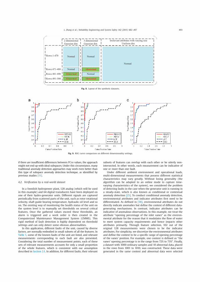
if there are insufficient differences between PCos values, the approachmight not end upwith ideal subspaces. Under this circumstance, manytraditional anomaly detection approaches may work even better thanthis type of subspace anomaly detection technique, as identified byprevious studies [11].
4.2. Verification by a real-world dataset
In a Swedish hydropower plant, 128 analog (which will be usedin this example) and 64 digital transducers have been deployed onone of their hydro-generator units. Different signals are capturedperiodically from scattered parts of the unit, such as rotor rotationalvelocity, shaft guide bearing temperature, hydraulic oil level and soon. The existing way of monitoring the health status of the unit onthe system level is to manually set thresholds on several criticalfeatures. Once the gathered values exceed these thresholds, analarm is triggered and a work order is then created in theComputerized Maintenance Management System (CMMS). Thisrigid method of fault detection is highly dependent on thresholdsettings and can only detect some obvious abnormalities.
In this application, different faults of the unit, caused by diversefactors, are normally embodied in small subsets of all the features. InTable 1, some of the known faults of the unit are listed, and relevantmeasurements corresponding to each fault are also presented.Considering the total number of measurement points, each of thesesets of relevant measurements accounts for only a small proportionof the whole features, which is consistent with our assumptiondescribed in Section 3.1. In addition, for different faults, their relevant
subsets of features can overlap with each other or be utterly non-intersected. In other words, each measurement can be indicative ofone or more than one fault.
Under different ambient environment and operational loads,multi-dimensional measurements that possess different statisticalcharacteristics may vary greatly. Without losing generality (thealgorithm can be adapted to an online mode to capture time-varying characteristics of the system), we considered the problemof detecting faults in the case when the generator unit is running ina steady-state, which is also known as conditional or contextualanomaly detection [25]. To conduct conditional anomaly detection,environmental attributes and indicator attributes first need to bedifferentiated. As defined in [38], environmental attributes do notdirectly indicate anomalies but define the context of different data-generating mechanisms. In contrast, indicator attributes can beindicative of anomalous observations. In this example, we treat theattribute “opening percentage of the inlet vanes” as the environ-mental attribute for the reason that it modulates the flow of waterto meet system capacity requirements and hence impacts otherattributes primarily. Through feature selection, 102 out of theoriginal 128 measurements were chosen to be the indicatorattributes. For simplicity, we discretize the environmental attributesand define the context to be a specific range of opening percentageof the vanes’ position. For example, one context is defined as “thevanes’ opening percentage is in the range from 72% to 73%”. Finally,a dataset with 1000 ordinary samples and 10 abnormal data, placedin the rows from 1001 to 1010, was constructed. These data weregenerated in the same context and abnormal data were selected
Rows:1-470
NormalRows:471-480
Rows:481-490
Rows:491-500
2-dimensionalGaussian dist.
3-dimensionalGaussian dist.
Irrelevant attributes with varying sizeUniform dist.
Normal Normal
Abnormal
Abnormal
AbnormalAbnormal
Normal
Normal
Fig. 8. Layout of the synthetic datasets.
Fig. 9. ROC curve comparison on different dimensionality settings.
L. Zhang et al. / Reliability Engineering and System Safety 142 (2015) 482–497 493

based on historical failure data which were not successfullydetected by the current method.
As expected, the algorithm yielded a satisfactory result whichcan be seen from Table 2. The topmost observations with thehighest overall local outlier score are listed in Table 2, in whichretained dimensions for each data point are also ranked by thesingle-dimensional local outlier scores in a descending order. The
output of the algorithm shows that 90% of the faults were detectedas the observations among the highest local outlier score list, andthe missed fault (observation 1002) has the overall local outlierscore 9.18 and was ranked at number 46. The 512th data point maybe considered as a false alarm even though it indeed deviates fromother points in the retained dimension by looking into the data.
Fig. 10. Local outlier score on each individual retained dimension.
Table 1Relevant attributes corresponding to some of the faults of the generator unit
Relevant measurements
Functional location Fault description Point Measurement description Unit
Shaft- coupling Loosened shaft coupling Ma43 Vibration of the turbine guide bearing (X side) mm/s– – M44 Vibration of the turbine guide bearing (Y side) mm/sShaft- guide bearing Too large bearing clearance M88 Vibration of the lower guide bearing (X side) μm– – M89 Vibration of the lower guide bearing (Y side) μmShaft- guide bearing Faulty guide bearing components M26 Temperature of the upper guide bearing (position 1) 1C– – M27 Temperature of the upper guide bearing (position 2) 1CGenerator- rotor Out-of-round rotor M35 Vibration of the lower guide bearing (X side) mm/s– – M36 Vibration of the lower guide bearing (Y side) mm/s– – M40 Vibration of the upper guide bearing (X side) mm/s– – M41 Vibration of the upper guide bearing (Y side) mm/sGenerator- magnetizer Thyristor discharger malfunction M9 Alternator voltage kVGenerator- cooling system- control Fault in the generator for cooling water control M83 Opening percentage of the fine water control valve %– – M84 Opening percentage of the stator control valve %Turbine- hydraulic pressure system Safety valve opens at a wrong pressure M50 Level of the control oil cm
– M51 Level of the pressure accumulator 1 cm– – M58 Pressure of the regulating oil barTurbine- hydraulic pressure system Improper oil level in the piston accumulator M51 Level of the pressure accumulator 1 cm– – M52 Level of the pressure accumulator 2 cm– – M53 Level of the pressure accumulator 3 cmTurbine- hydraulic pressure system Regular pump does not deliver the required capacity M58 Pressure of the regulating oil bar
a M represents measurement points.
L. Zhang et al. / Reliability Engineering and System Safety 142 (2015) 482–497494
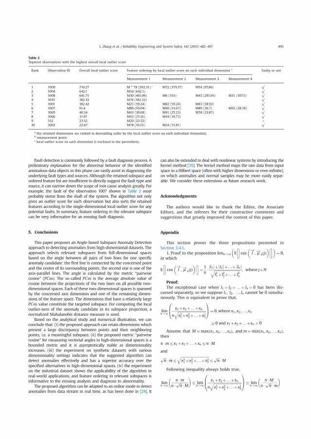
Fault detection is commonly followed by a fault diagnosis process. Apreliminary explanation for the abnormal behavior of the identifiedanomalous data objects in this phase can vastly assist in diagnosing theunderlying fault types and sources. Although the retained subspace andordered feature list are insufficient to directly suggest the fault type andsource, it can narrow down the scope of root cause analysis greatly. Forexample, the fault of the observation 1007 shown in Table 2 mostprobably stems from the shaft of the system. The algorithm not onlygives an outlier score for each observation but also sorts the retainedfeatures according to the single-dimensional local outlier score for anypotential faults. In summary, feature ordering in the relevant subspacecan be very informative for an ensuing fault diagnosis.
5. Conclusions
This paper proposes an Angle-based Subspace Anomaly Detectionapproach to detecting anomalies from high-dimensional datasets. Theapproach selects relevant subspaces from full-dimensional spacesbased on the angle between all pairs of two lines for one specificanomaly candidate: the first line is connected by the concerned pointand the center of its surrounding points; the second one is one of theaxis-parallel lines. The angle is calculated by the metric “pairwisecosine” (PCosÞ. The so-called PCos is the average absolute value ofcosine between the projections of the two lines on all possible two-dimensional spaces. Each of these two-dimensional spaces is spannedby the concerned axis dimension and one of the remaining dimen-sions of the feature space. The dimensions that have a relatively largePCos value constitute the targeted subspace. For computing the localoutlier-ness of the anomaly candidate in its subspace projection, anormalized Mahalanobis distance measure is used.
Based on the analytical study and numerical illustration, we canconclude that: (i) the proposed approach can retain dimensions whichpresent a large discrepancy between points and their neighboringpoints, i.e. a meaningful subspace. (ii) the proposed metric “pairwisecosine” for measuring vectorial angles in high-dimensional spaces is abounded metric and it is asymptotically stable as dimensionalityincreases. (iii) the experiment on synthetic datasets with variousdimensionality settings indicates that the suggested algorithm candetect anomalies effectively and has a superior accuracy over thespecified alternatives in high-dimensional spaces. (iv) the experimenton the industrial dataset shows the applicability of the algorithm inreal-world applications, and feature ordering in relevant subspaces isinformative to the ensuing analysis and diagnosis to abnormality.
The proposed algorithm can be adapted to an onlinemode to detectanomalies from data stream in real time, as has been done in [24]. It
can also be extended to deal with nonlinear systems by introducing thekernel method [39]. The kernel method maps the raw data from inputspace to a Hilbert space (oftenwith higher dimensions or even infinite),on which anomalies and normal samples may be more easily separ-able. We consider these extensions as future research work.
Acknowledgments
The authors would like to thank the Editor, the AssociateEditors, and the referees for their constructive comments andsuggestions that greatly improved the content of this paper.
Appendix
This section proves the three propositions presented inSection 3.4.1.
1. Proof to the proposition limn-1 E cos l!
; μ!n jð Þ� �����
����� � �
¼ 0,in which
E cos l!
; μ!n jð Þ� �����
�����
¼ 1nUl1�� ��þ l2
�� ��þ…þ ln�� ��ffiffiffiffiffiffiffiffiffiffiffiffiffiffiffiffiffiffiffiffiffiffiffiffiffiffiffiffiffiffi
l21þ l22þ…þ l2n
q ; where jAN
Proof:The exceptional case when l1 ¼ l2 ¼…¼ ln ¼ 0 has been dis-
cussed separately, so we suppose l1; l2; …; ln cannot be 0 simulta-neously. This is equivalent to prove that,
limn-1
x1þx2þ…þxn
nffiffiffiffiffiffiffiffiffiffiffiffiffiffiffiffiffiffiffiffiffiffiffiffiffiffiffiffiffiffiffiffiffix21þx22þ…þx2n
q0B@
1CA¼ 0;where x1; x2;…; xn
Z0 and x1þx2þ…þxn40
Assume that M¼max x1; x2;…; xnf g, andm¼min x1; x2;…; xnf g,then
nUmrx1þx2þ…þxnrnUM
and
ffiffiffin
pUmr
ffiffiffiffiffiffiffiffiffiffiffiffiffiffiffiffiffiffiffiffiffiffiffiffiffiffiffiffiffiffiffiffiffix21þx22þ…þx2n
qr
ffiffiffin
pUM
Following inequality always holds true,
limn-1
nUmnU
ffiffiffin
pUM
� �r lim
n-1x1þx2þ…þxn
nffiffiffiffiffiffiffiffiffiffiffiffiffiffiffiffiffiffiffiffiffiffiffiffiffiffiffiffiffiffiffiffiffix21þx22þ…þx2n
q0B@
1CAr lim
n-1nUM
nUffiffiffin
pUm
� �
Table 2Topmost observations with the highest overall local outlier score
Rank Observation ID Overall local outlier score Feature ordering by local outlier score on each individual dimension a Faulty or not
Measurement 1 Measurement 2 Measurement 3 Measurement 4
1 1009 710.27 M b 79 (592.31) c M72 (379.57) M54 (97.86) √2 1004 642.1 M54 (642.1) √3 1008 641.75 M30 (401.96) M6 (355) M43 (291.95) M31 (197.5) √4 1010 182.32 M74 (182.32) √5 1001 102.42 M23 (59.24) M82 (59.24) M83 (58.92) √6 1007 91.4 M88 (59.04) M90 (55.67) M89 (30.7) M92 (28.76) √7 1005 46.34 M43 (30.68) M91 (25.23) M58 (23.87) √8 1006 31.97 M43 (25.16) M44 (19.73) √9 512 23.52 M20 (23.52) �10 1003 22.67 M78 (16.15) M24 (15.91) √
a the retained dimensions are ranked in descending order by the local outlier score on each individual dimension;b measurement point;c local outlier score on each dimension is enclosed in the parenthesis.
L. Zhang et al. / Reliability Engineering and System Safety 142 (2015) 482–497 495
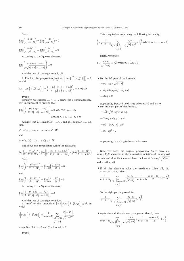
Since,
limn-1
nUmnU
ffiffiffin
pUM
� �¼ lim
n-1mffiffiffin
pUM
� �¼ 0
limn-1
nUMnU
ffiffiffin
pUm
� �¼ lim
n-1Mffiffiffin
pUm
� �¼ 0
According to the Squeeze theorem,
limn-1
x1þx2þ…þxn
nffiffiffiffiffiffiffiffiffiffiffiffiffiffiffiffiffiffiffiffiffiffiffiffiffiffiffiffiffiffiffiffiffix21þx22þ…þx2n
q0B@
1CA¼ 0
And the rate of convergence is 1=ffiffiffin
p.
2. Proof to the proposition limn-1
Var cos l!
; μ!n jð Þ� �����
����� � �
¼ 0,in which
Var cos l!
; μ!n jð Þ� �����
�����
¼ 1n� l1�� ��þ l2
�� ��þ…þ ln�� �� �2
n2 U l21þ l22þ…þ l2n� ; where jAN
Proof:Similarly, we suppose l1; l2; …; ln cannot be 0 simultaneously.
This is equivalent to proving that,
limn-1
1n� x1þx2þ…þxnð Þ2n2 x21þx22þ…þx2n �
" #¼ 0;where x1; x2;…; xn
Z0 and x1þx2þ…þxn40
Assume that M¼max x1; x2;…; xnf g, and m¼min x1; x2;…; xnf g,then
n2 Um2r x1þx2þ…þxnð Þ2rn2 UM2
and,
nUm2r x21þx22þ…þx2n �
rnUM2
The above two inequalities suffice the following,
limn-1
1n� n2 UM2
n2 UnUm2
!r lim
n-11n� x1þx2þ…þxnð Þ2n2 x21þx22þ…þx2n �
" #r lim
n-11n� n2 Um2
n2 UnUM2
� �
Since,
limn-1
1n� n2 UM2
n2 UnUm2
!¼ lim
n-11n
1�M2
m2
!¼ 0
and,
limn-1
1n� n2 Um2
n2 UnUM2
� �¼ lim
n-11n
1�m2
M2
� �¼ 0
According to the Squeeze theorem,
limn-1
1n� x1þx2þ…þxnð Þ2n2 x21þx22þ…þx2n �
" #¼ 0
And the rate of convergence is 1=n.3. Proof to the proposition 1
2oE PCos l!
; μ!n jð Þ� ��
rffiffi2
p2 , in
which
E PCos l!
; μ!n jð Þ� ��
¼ 1nUðn�1Þ
Xj; j� AN
j� a j
l#j��� ���þ l#j�
��� ���ffiffiffiffiffiffiffiffiffiffiffiffiffiffiffiffiffil#2j þ l#2j�
q ;
where N¼ 1;2;…;nf g; and l#j 40 for all jAN
Proof:
This is equivalent to proving the following inequality,
12o 1
nU n�1ð ÞX
i; jA 1;2;…nf gia j
xiþxjffiffiffiffiffiffiffiffiffiffiffiffiffiffix2i þx2j
q rffiffiffi2
p
2;where x1; x2;…; xn40
Firstly, we prove
1o xiþxjffiffiffiffiffiffiffiffiffiffiffiffiffiffix2i þx2j
q rffiffiffi2
p;where xi40; xj40
� For the left part of the formula,
( ðxiþxjÞ4ffiffiffiffiffiffiffiffiffiffiffiffiffiffix2i þx2j
q
( ðx2i þ2xixjþx2j Þ4x2i þx2j
( 2xixj40
Apparently, 2xixj40 holds true when xi40 and xj40� For the right part of the formula,
(ffiffiffi2
pUffiffiffiffiffiffiffiffiffiffiffiffiffiffix2i þx2j
qZ ðxiþxjÞ
( 2Uðx2i þx2j ÞZ ðxiþxjÞ2
( ðx2i �2xixjþx2j ÞZ0
( ðxi�xjÞ2Z0
Apparently, ðxi�xjÞ2Z0 always holds true.
Now, we prove the original proposition. Since there arenUðn�1Þ=2 elements in the summation notation of the original
formula and all of the elements have the form of ðxiþxjÞ=ffiffiffiffiffiffiffiffiffiffiffiffiffiffix2i þx2j
qand xi40; xj40.
� if all the elements take the maximum valueffiffiffi2
p, i.e.
x1 ¼ x2 ¼…¼ xn , then
1nU n�1ð Þ
Xi; jA 1;2;…nf g
ia j
xiþxjffiffiffiffiffiffiffiffiffiffiffiffiffiffix2i þx2j
q ¼ 1nU n�1ð ÞU
nU n�1ð Þ2
Uffiffiffi2
p¼
ffiffiffi2
p
2
So the right part is proved, i.e.
1nU n�1ð Þ
Xi; jA 1;2;…nf g
ia j
xiþxjffiffiffiffiffiffiffiffiffiffiffiffiffiffix2i þx2j
q rffiffiffi2
p
2
� Again since all the elements are greater than 1, then
1nU n�1ð Þ
Xi; jA 1;2;…nf g
ia j
xiþxjffiffiffiffiffiffiffiffiffiffiffiffiffiffix2i þx2j
q 41
nU n�1ð ÞUnU n�1ð Þ
2U1¼ 1
2
L. Zhang et al. / Reliability Engineering and System Safety 142 (2015) 482–497496

So the left part is proved, i.e.
1nU n�1ð Þ
Xi; jA 1;2;…nf g
ia j
xiþxjffiffiffiffiffiffiffiffiffiffiffiffiffiffix2i þx2j
q 412
Thus, the original proposition is right.
References
[1] Montgomery DC. Big data and the quality profession. Qual Reliab Eng Int2014;30(4):447.
[2] Sribar VT, Feinberg D, Gall N, Lapkin A, Beyer MA., Big Data is only thebeginning of extreme information management. Gartner, Stamford, CT; 2011.
[3] Zhai Y, Ong Y-S, Tsang IW. The emerging big dimensionality. Comput IntellMag IEEE 2014;9(3):14–26.
[4] Meeker WQ, Hong Y. Reliability meets big data: opportunities and challenges.Qual Eng 2014;26(1):102–16.
[5] Domingos P. A few useful things to know about machine learning. CommunACM 2012;55(10):78–87.
[6] Göb R. Discussion of reliability meets big data: opportunities and challenges.Qual Eng 2013;26(1):121–6.
[7] Hawkins DM. Identification of outliers. 1980.[8] Guo B, Wang BX, Xie M. A study of process monitoring based on inverse
Gaussian distribution. Comput Ind Eng 2014;76:49–59.[9] Baraldi P, Roozbeh R-F, Zio E. Classifier-ensemble incremental-learning pro-
cedure for nuclear transient identification at different operational conditions.Reliab Eng Syst Saf 2011;96(4):480–8.
[10] Albaghdadi M, Briley B, Evens M. Event storm detection and identification incommunication systems. Reliab Eng Syst Saf 2006;91(5):602–13.
[11] Houle ME, Kriegel H-P, Kröger P, Schubert E, Zimek A. Can shared-neighbordistances defeat the curse of dimensionality? Scientific and Statistical Data-base Management. Berlin Heidelberg: Springer; 2010. p. 482–500.
[12] Zimek A, Schubert E, Kriegel H-P. A survey on unsupervised outlier detectionin high-dimensional numerical data,. Stat Anal Data Min 2012;5(5):363–87.
[13] Dai X, Gao Z. From model, signal to knowledge: a data-driven perspective offault detection and diagnosis. IEEE Trans Ind Inf 2013;9(4):2226–38.
[14] Zhong S, Langseth H, Nielsen TD. A classification-based approach to monitor-ing the safety of dynamic systems,. Reliab Eng Syst Saf 2014;121:61–71.
[15] Rocco S. CM, Zio E. A support vector machine integrated system for theclassification of operation anomalies in nuclear components and systems.Reliab Eng Syst Saf 2007;92(5):593–600.
[16] Tamilselvan P, Wang P. Failure diagnosis using deep belief learning basedhealth state classification. Reliab Eng Syst Saf 2013;115:124–35.
[17] Traore M, Chammas A, Duviella E. Supervision and prognosis architecturebased on dynamical classification method for the predictive maintenance ofdynamical evolving systems. Reliab Eng Syst Saf 2015;136:120–31.
[18] Li F, Church G, Janakiram M, Gholston H, Runger G. Fault detection for batchmonitoring and discrete wavelet transforms,. Qual Reliab Eng Int 2011;27(8):999–1008.
[19] Huang S-P, Chiu C-C. Process monitoring with ICA-based signal extractiontechnique and CART approach. Qual Reliab Eng Int 2009;25(5):631–43.
[20] Hwang W-Y, Lee J-S. Shifting artificial data to detect system failures. Int TransOper Res 2015;22(2):363–78.
[21] Lee J-M, Qin SJ, Lee I-B. Fault detection and diagnosis based on modifiedindependent component analysis. AIChE J 2006;52(10):3501–14.
[22] Lee J, Kang B, Kang S-H. Integrating independent component analysis andlocal outlier factor for plant-wide process monitoring. J Process Control2011;21(7):1011–21.
[23] Zhao Y, Wang S, Xiao F. Pattern recognition-based chillers fault detectionmethod using support vector data description (SVDD). Appl Energy2013;112:1041–8.
[24] Ma Y, Shi H, Ma H, Wang M. Dynamic process monitoring using adaptive localoutlier factor. Chemom Intell Lab Syst 2013;127:89–101.
[25] Chandola V, Banerjee A, Kumar V. Anomaly detection: a survey. ACM ComputSurv 2009;41(3):1–72.
[26] Li J, Huang K-Y, Jin J, Shi J. A survey on statistical methods for health care frauddetection. Health Care Manag Sci 2008;11(3):275–87.
[27] Knorr EM, Ng RT, Tucakov V. Distance-based outliers: algorithms andapplications,. VLDB J Int J Very Large Data Bases 2000;8(3–4):237–53.
[28] Kriegel H-P, Zimek A. Angle-based outlier detection in high-dimensional data.In: Proceedings of the 14th ACM SIGKDD international conference on Knowl-edge discovery and data mining; 2008. p. 444–52.
[29] Breunig MM, Kriegel H, Ng RT, Sander J. LOF : identifying density-based localoutliers. ACM Sigmod Rec 2000;29(2):93–104.
[30] Beyer K, Goldstein J, Ramakrishnan R, Shaft U. When is ‘nearest neighbor’meaningful? Database Theory—ICDT'99. Berlin Heidelberg: Springer; 1999. p.217–235.
[31] Piao C, Huang Z, Su L, Lu S. Research on outlier detection algorithm forevaluation of battery system safety. Adv Mech Eng 2014;2014:1–8.
[32] Aggarwal CC, Yu PS. Outlier detection for high dimensional data. ACM SIGMODRec 2001;30(2):37–46.
[33] Lazarevic A, Kumar V. Feature bagging for outlier detection. In: Proceeding ofthe eleventh ACM SIGKDD international conference on knowledge discoveryin data mining; 2005. p. 157–66.
[34] Kriegel H, Kröger P, Schubert E, Zimek A. Outlier detection in axis-parallelsubspaces of high dimensional data. Advances in Knowledge Discovery andData Mining. Berlin Heidelberg: Springer; 2009. p. 831–8.
[35] Ye M, Li X, Orlowska ME. Projected outlier detection in high-dimensionalmixed-attributes data set. Expert Syst Appl 2009;36(3):7104–13.
[36] Ayad H, Kamel M. Finding natural clusters using multi-clusterer combinerbased on shared nearest neighbors. Multiple classifier systems. Berlin Heidel-berg: Springer; 2003. p. 166–75.
[37] Cai T, Fan J, Jiang T. Distributions of angles in random packing on spheres. JMach Learn Res 2013;14(1):1837–64.
[38] Song X, Wu M, Jermaine C, Ranka S. Conditional anomaly detection. IEEE TransKnowl Data Eng 2007;19(5):631–45.
[39] Zhang Y, Qin SJ. Improved nonlinear fault detection technique and statisticalanalysis. AIChE J 2008;54(12):3207–20.
L. Zhang et al. / Reliability Engineering and System Safety 142 (2015) 482–497 497
PAPER II
Sliding Window-based Fault Detection from High-
dimensional Data Streams
Zhang, L., Lin, J. and Karim, R., 2016. Sliding Window-based Fault Detection from High-dimensional Data Streams. IEEE Transactions on Systems, Man, and Cybernetics: System, Published online.
http://dx.doi.org/10.1109/TSMC.2016.2585566

This article has been accepted for inclusion in a future issue of this journal. Content is final as presented, with the exception of pagination.
IEEE TRANSACTIONS ON SYSTEMS, MAN, AND CYBERNETICS: SYSTEMS 1
Sliding Window-Based Fault Detection FromHigh-Dimensional Data Streams
Liangwei Zhang, Jing Lin, Member, IEEE, and Ramin Karim
Abstract—High-dimensional data streams are becomingincreasingly ubiquitous in industrial systems. Efficient detec-tion of system faults from these data can ensure the reliabilityand safety of the system. The difficulties brought about by highdimensionality and data streams are mainly the “curse of dimen-sionality” and concept drifting, and one current challenge isto simultaneously address them. To this purpose, this paperpresents an approach to fault detection from nonstationary high-dimensional data streams. An angle-based subspace anomalydetection approach is proposed to detect low-dimensional sub-space faults from high-dimensional datasets. Specifically, it selectsfault-relevant subspaces by evaluating vectorial angles and com-putes the local outlier-ness of an object in its subspace projection.Based on the sliding window strategy, the approach is furtherextended to an online mode that can continuously monitor sys-tem states. To validate the proposed algorithm, we comparedit with the local outlier factor-based approaches on artificialdatasets and found the algorithm displayed superior accuracy.The results of the experiment demonstrated the efficacy of theproposed algorithm. They also indicated that the algorithm hasthe ability to discriminate low-dimensional subspace faults fromnormal samples in high-dimensional spaces and can be adap-tive to the time-varying behavior of the monitored system. Theonline subspace learning algorithm for fault detection would bethe main contribution of this paper.
Index Terms—Big data analytics, fault detection, high-dimensional data, stream data mining.
NOMENCLATURE
Acronyms
ABSAD Angle-based subspace anomaly detection.AUC Area under curve.EWPCA Exponentially weighted principal compo-
nent analysis.FNR False negative rate.FPR False positive rate.ICA Independent component analysis.KDE Kernel density estimation.LOF Local outlier factor.LOS Local outlier score.MSPC Multivariate statistical process control.
Manuscript received May 16, 2015; revised September 2, 2015 andNovember 2, 2015; accepted June 19, 2016. This paper was recommended byAssociate Editor G. Biswas. (Corresponding author: Liangwei Zhang.)The authors are with the Division of Operation and Maintenance
Engineering, Luleå University of Technology, Luleå SE-97187, Sweden(e-mail: [email protected]).Color versions of one or more of the figures in this paper are available
online at http://ieeexplore.ieee.org.Digital Object Identifier 10.1109/TSMC.2016.2585566
PCA Principal component analysis.ROC Receiver operating characteristic.RPCA Recursive PCA.SNN Shared nearest neighbors.SOD Subspace outlier detection.SPE Squared prediction error.SWPCA Sliding window PCA.TPR True positive rate.X Design matrix.m Number of data points (rows) in X.n Number of dimensions (columns) in X.N Index set of feature space {1, . . . , n}.LOS Vector of LOSs.i ith data point (row) in X, or the ith
window.j jth element of a vector, or the jth dimen-
sion (column) of a matrix.v Vector representation of a point.p Data point (outlier candidate).RP Set of reference points of a point.q Data point represents the geometric center
of all the points in RP(p).l Line connected through two points (e.g., p
and q).dist(·, ·) Metric for measuring the distance between
two points.kNN(i) k nearest neighbor list of the ith point.SimSNN Similarity value of two points derived by
the SNN method.SNNs s nearest neighbor list of a point derived
by the SNN method.PCos(�l, �μn( j)) Average absolute value of cosine between
line l and the jth axis in all possible com-binations of the 2-D spaces ( j, j−), wherej− ∈ N\{ j}.
d Number of retained dimensions of a point.G Threshold for singling out large PCos
values.K(·) Kernel function.h Smoothing parameter in the KDE.W(i) All the samples preserved in the ith win-
dow profile.kNN-list(i) Set of sets, containing the k nearest neigh-
bors of every sample in the ith window.k-Dist(i) Vector, recording the k-distance of each
sample in the ith window.CL(i) Scalar, the control limit of the ith
window.
2168-2216 c© 2016 IEEE. Personal use is permitted, but republication/redistribution requires IEEE permission.See http://www.ieee.org/publications_standards/publications/rights/index.html for more information.
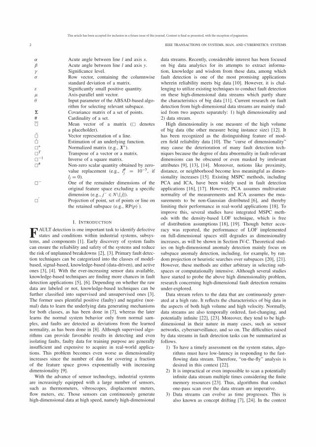
This article has been accepted for inclusion in a future issue of this journal. Content is final as presented, with the exception of pagination.
2 IEEE TRANSACTIONS ON SYSTEMS, MAN, AND CYBERNETICS: SYSTEMS
α Acute angle between line l and axis x.β Acute angle between line l and axis y.γ Significance level.σ Row vector, containing the columnwise
standard deviation of a matrix.ε Significantly small positive quantity.μ Axis-parallel unit vector.θ Input parameter of the ABSAD-based algo-
rithm for selecting relevant subspace.� Covariance matrix of a set of points.# Cardinality of a set.� Mean vector of a matrix (� denotes
a placeholder).�� Vector representation of a line.� Estimation of an underlying function.�
∗ Normalized matrix (e.g., X∗).�T Transpose of a vector or a matrix.
�−1 Inverse of a square matrix.
�# Non-zero scalar quantity obtained by zero-
value replacement (e.g., l#j = 10−5, iflj = 0).
�− One of the remainder dimensions of the
original feature space excluding a specificdimension (e.g., j− ∈ N\{ j}).
�′
Projection of point, set of points or line onthe retained subspace (e.g., RP(p)
′).
I. INTRODUCTION
FAULT detection is one important task to identify defectivestates and conditions within industrial systems, subsys-
tems, and components [1]. Early discovery of system faultscan ensure the reliability and safety of the systems and reducethe risk of unplanned breakdowns [2], [3]. Primary fault detec-tion techniques can be categorized into the classes of model-based, signal-based, knowledge-based (data-driven), and activeones [3], [4]. With the ever-increasing sensor data available,knowledge-based techniques are finding more chances in faultdetection applications [5], [6]. Depending on whether the rawdata are labeled or not, knowledge-based techniques can befurther classified into supervised and unsupervised ones [3].The former uses plentiful positive (faulty) and negative (nor-mal) data to learn the underlying data generating mechanismsfor both classes, as has been done in [7], whereas the laterlearns the normal system behavior only from normal sam-ples, and faults are detected as deviations from the learnednormality, as has been done in [8]. Although supervised algo-rithms can provide favorable results in detecting and evenisolating faults, faulty data for training purpose are generallyinsufficient and expensive to acquire in real-world applica-tions. This problem becomes even worse as dimensionalityincreases since the number of data for covering a fractionof the feature space grows exponentially with increasingdimensionality [9].With the advance of sensor technology, industrial systems
are increasingly equipped with a large number of sensors,such as thermometers, vibroscopes, displacement meters,flow meters, etc. Those sensors can continuously generatehigh-dimensional data at high speed, namely high-dimensional
data streams. Recently, considerable interest has been focusedon big data analytics for its attempts to extract informa-tion, knowledge and wisdom from these data, among whichfault detection is one of the most promising applicationswherein reliability meets big data [10]. However, it is chal-lenging to utilize existing techniques to conduct fault detectionon these high-dimensional data streams which partly sharethe characteristics of big data [11]. Current research on faultdetection from high-dimensional data streams are mainly stud-ied from two aspects separately: 1) high dimensionality and2) data stream.High dimensionality is one measure of the high volume
of big data (the other measure being instance size) [12]. Ithas been recognized as the distinguishing feature of mod-ern field reliability data [10]. The “curse of dimensionality”may cause the deterioration of many fault detection tech-niques because the degree of data abnormality in fault-relevantdimensions can be obscured or even masked by irrelevantattributes [9], [13], [14]. Moreover, notions like proximity,distance, or neighborhood become less meaningful as dimen-sionality increases [15]. Existing MSPC methods, includingPCA and ICA, have been widely used in fault detectionapplications [16], [17]. However, PCA assumes multivariatenormality of the measurements and ICA assumes the mea-surements to be non-Gaussian distributed [6], and therebylimiting their performance in real-world applications [18]. Toimprove this, several studies have integrated MSPC meth-ods with the density-based LOF technique, which is freeof distribution assumptions [18], [19]. Though better accu-racy was reported, the performance of LOF implementedon full-dimensional spaces still degrades as dimensionalityincreases, as will be shown in Section IV-C. Theoretical stud-ies on high-dimensional anomaly detection mainly focus onsubspace anomaly detection, including, for example, by ran-dom projection or heuristic searches over subspaces [20], [21].However, these methods are either arbitrary in selecting sub-spaces or computationally intensive. Although several studieshave started to probe the above high dimensionality problem,research concerning high-dimensional fault detection remainsunder-explored.Data stream refers to the data that are continuously gener-
ated at a high rate. It reflects the characteristics of big data inthe aspects of both high volume and high velocity. Normally,data streams are also temporally ordered, fast-changing, andpotentially infinite [22], [23]. Moreover, they tend to be high-dimensional in their nature in many cases, such as sensornetworks, cybersurveillance, and so on. The difficulties raisedby data streams in fault detection tasks can be summarized asfollows.1) To have a timely assessment on the system status, algo-
rithms must have low-latency in responding to the fast-flowing data stream. Therefore, “on-the-fly” analysis isdesired in this context [22].
2) It is impractical or even impossible to scan a potentiallyinfinite data stream multiple times considering the finitememory resources [23]. Thus, algorithms that conductone-pass scan over the data stream are imperative.
3) Data streams can evolve as time progresses. This isalso known as concept drifting [7], [24]. In the context
This article has been accepted for inclusion in a future issue of this journal. Content is final as presented, with the exception of pagination.
ZHANG et al.: SLIDING WINDOW-BASED FAULT DETECTION FROM HIGH-DIMENSIONAL DATA STREAMS 3
of fault detection, the behavior of systems can varyover time—time-varying—due to many reasons, suchas seasonal fluctuation, equipment aging, process drift-ing, and so forth. Fault detection algorithms need to beadaptive to this time-varying behavior of the monitoredsystem [25]. A large portion of online fault detectionalgorithms were extended from existing ones for thepurpose of monitoring data streams, such as the RPCA,EWPCA, and SWPCA [26]–[28]. The key to these algo-rithms is that the learning model should be refined,enhanced, and personalized while the stream evolves soas to accommodate the natural drift in the data stream.In spite of the extensive studies of fault detectiontechniques, fault detection applications which specifi-cally address the challenges imposed by data streamproperties are also limited [29].
Today, the capability of fault detection techniques in simul-taneously addressing the challenges associated with highdimensionality and data streams remains limited. To solve theabove problems, this paper proposes an unsupervised approachto fault detection from high-dimensional data streams withtime-varying characteristics.1) First, in considering the high-dimensional challenges in
fault detection tasks, an ABSAD approach is proposed.The ABSAD approach selects fault-relevant subspacesby evaluating vectorial angles and computes the localoutlier-ness of an object in its subspace projection bya normalized Mahalanobis distance measure.
2) Second, aiming to detect faults from data stream withtime-varying characteristics, the ABSAD approach isextended to an online mode based on the sliding windowstrategy. According to the requirements of the ABSADapproach, several necessities (mean vector, KNN list,etc.) are identified and incorporated into the windowprofile of the sliding window ABSAD algorithm.
The updating mechanisms to these necessities are inves-tigated and thoroughly described. To validate the proposedalgorithm, we compared it with the LOF-based approacheson artificial datasets and found the algorithm displayedsuperior accuracy. The results of the experiment demon-strated the efficacy of the proposed algorithm. They alsoindicated that the algorithm is able to discriminate low-dimensional subspace faults from normal samples in high-dimensional spaces and can be adaptive to the time-varyingbehavior of the monitored system. This paper contributes toa new online subspace learning algorithm for detecting faultsfrom nonstationary systems. To the best of our knowledge,no online fault detection algorithms utilizing angle evalu-ation to select fault-relevant subspaces have been reportedto date.The rest of this paper proceeds as follows. In Section II,
we propose an ABSAD approach with the aim of handlinghigh dimensionality challenges in anomaly detection tasks. Toaddress the challenges associated with data stream mining,Section III extends the ABSAD approach to an online modebased on the sliding window strategy. Section IV evaluatesthe proposed algorithm on synthetic datasets and comparesit with other alternatives. Finally, the study is concluded inSection V.
II. ANGLE-BASED SUBSPACE ANOMALY
DETECTION APPROACH
To mitigate the impact exerted by anomaly-irrelevantattributes, the degree of deviation of a data point from itsneighboring points (i.e., local outlier-ness) should be com-puted in a meaningful subspace instead of the full-dimensionalspace. The subspace is said to be meaningful in the sensethat it should capture most information with regard to the dis-cordance of an object to its adjacent ones. To this end, wepropose an ABSAD approach to exploring and selecting low-dimensional, axis-parallel subspaces that can retain a largeportion of points’ local outlier-ness. For each data instance,the degree of deviation from its neighborhood is evaluated onthe obtained subspace. A local outlier score is then computedfor these points indicating whether it is abnormal or not. Moretheoretical discussions to this approach can be referred to [30].In the following, we describe the ABSAD approach. We
first elucidate the model assumption, and then introduce thestructure of the ABSAD approach. Subsequently, we elaboratethe main steps of the approach respectively and integrate theminto a single algorithm.
A. Model Assumption
The separability of different data generation mechanismsmay not necessarily depend on the amount of data dimen-sionality, but instead on the ratio of relevant versus irrelevantattributes [13]. In cases where the relevant attributes accountfor a large proportion of the whole dimensions, the separa-bility among different mechanisms tends to increase, whichmeans traditional techniques are still valid and may workeven better in high-dimensional spaces. Conversely, when rel-evant attributes are in a minority of the whole dimensions,the curse of dimensionality would hamper anomaly detec-tion tasks. This paper attempts to address the problem of thelatter case. Hereinafter, we assume the number of anomaly-relevant attributes is in a minority of all the attributes in thefeature space.
B. Computational Procedure
The computational procedure of the ABSAD approach ispresented in Fig. 1. The first step, data preparation, usuallycomprises data acquisition, data cleaning, feature selection,and other preprocessing processes. The complexity of this stepmainly depends on the quality of the collected raw data. Sincethis step is highly dependent on various applications and plen-tiful studies have been conducted specifically on these topics,the remainder of this section will instead focus on the corepart of the approach (enclosed by the outer box in Fig. 1).In the following, we define X (X ⊆ Rm×n) as the
design matrix. Each row of the matrix represents a data point(also known as data instance, object or observation) in an-dimensional feature space N, where N = {1, . . . , n} andn ≥ 2. The objective of this approach is to define a functionwhich maps X to a real-valued vector LOS, i.e., f : X →LOS,where LOS(i) is the ith point’s local outlier score. To evaluatethe local outlier-ness of a particular data point p, a set of refer-ence points RP(p) of p needs to be specified beforehand. Theset RP(p) reflects the notion of locality. Additionally, a dis-tance metric dist(p, o) (e.g., one of the Lp norms) measuring

This article has been accepted for inclusion in a future issue of this journal. Content is final as presented, with the exception of pagination.
4 IEEE TRANSACTIONS ON SYSTEMS, MAN, AND CYBERNETICS: SYSTEMS
Fig. 1. Computational procedure of the ABSAD approach.
the distance between any two points p and o is required whenderiving the set RP(p).
C. Feature Normalization
The feature normalization step is to standardize the rangeof values in different features. It is imperative to conduct thisstep because those features with mean or variance that areorders of magnitude larger than others are likely to dominatesucceeding computations. In anomaly detection applications,we recommend the use of the Z-score normalization insteadof the min–max scaling considering the latter may suppressthe effect of abnormality which might deviate from our inten-tion. The Z-score method normalizes the design matrix X toa dimensionless matrix X∗ with zero mean and unit variance.The ith row of X∗ can be calculated as follows:
x∗i = xi − x
σ, for all i ∈ {1, 2, . . . ,m} (1)
where x is the columnwise mean vector of the design matrixand σ is the columnwise standard deviation vector.
D. Derivation of Reference Sets
The implication of locality needs to be defined in localoutlier detection approaches, i.e., to determine the set ofreference points. In low-dimensional spaces, distance-basedmeasures are frequently used to explore the vicinity of a point.However, as stated before, notions like proximity, distance,or neighborhood become less meaningful in high-dimensionalspaces. To cope with this problem, an alternative series ofmethods, which introduce a secondary measure based onthe rankings of data instances produced by a primary sim-ilarity measure, were proposed. Among these methods, theSNN approach is the most common one. The applicability ofSNN in high-dimensional spaces has been empirically justifiedin [13] and it was adopted in several other related researchprojects [21], [31].The main idea of the SNN method is that two points gener-
ated by the same mechanism should have more overlap in theirnearest neighbor list, and vice versa. Specifically, SNN mea-sures the similarity of two points as the number of common
nearest neighbors which are derived from a primary measure.Prior to calculating the SNN similarity, a primary measure isneeded to specify the nearest neighbors for all the points. Theprimary measure can be of any traditional similarity measure(such as Lp norm or the cosine measure). Notably, the rankingof data instances derived by the primary measure is typi-cally still meaningful in high-dimensional spaces even thoughthe contrast of distance measure has deteriorated. Supposethe k nearest neighbor set of point p is denoted as kNN(p).Then, the SNN similarity between points p and q can berepresented as
SimSNN(p, q) = #{kNN(p) ∩ kNN(q)}. (2)
Here the sign # returns the cardinality of the intersectionbetween sets kNN(p) and kNN(q). Notably, the above equa-tion only computes the similarity between pairwise points.To derive a secondary nearest neighbor list SNN(p), weneed to sort all the SNN similarity values of point p withrespect to other remaining points in X in descending order.The first s elements with largest SNN similarity values in theset SNN(p), i.e., SNNs(p), constitute the reference set RP(p).
E. Selection of Relevant Subspaces
The general idea as to which dimensions should be retainedto constitute the anomaly-relevant subspaces is elaborated asbelow. The example shown in Fig. 2 gives us an intuitionon selecting relevant subspaces. In a 2-D case as shown inFig. 2(a), the set RP(p) (enclosed by an ellipse) contains thenearest neighbors of an outlier candidate p (black cross). InFig. 2(b), the geometrical center of RP(p) is calculated andrepresented by the point q (red circle). Points p and q areconnected to form the line l (red solid line). In consideringwhich of the 2-D (x and y) p deviates significantly from itsreference points, we can evaluate the angle α between linel and the x-axis, and β between line l and the y-axis (bothα and β are acute angle). Intuitively, the dimension whichhas a fairly small angle with line l should be retained inthe relevant subspace. In this case, angle α is small indicat-ing that line l is nearly parallel to the x-axis, whereas β ismarkedly larger implying that line l is almost perpendicularto the y-axis. Consequently, the dimension on the x-axis isretained and the dimension on the y-axis is excluded. Now,as shown in Fig. 2(c), we can project the original data pointsonto the x-axis and compute the local outlier-ness of p in thissubspace.Before generalizing the selection of relevant subspaces in
high-dimensional spaces, let us define some more notations.Formally, let �μn( j), j ∈ N denote the jth axis-parallel unitvector in a n-dimensional space. Concretely, �μn( j) is a n× 1vector with the jth element one and others zero. Further, letvp and vq be the vector representation of point p and q,respectively, and vq is the mean of all the points in RP(p).Correspondingly, the vector representation of line l can bewritten as �l, and �l = vp − vq. Here we define the jth elementof vector �l as lj, i.e., �l = [l1, l2, . . . , ln]T .An alternative way to measure the angle between two lines
is by the absolute value of the cosine between the two cor-responding vectors. Let |cos(�l, �μn( j))| denote the absolute
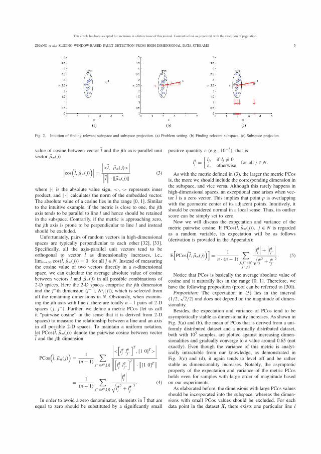
This article has been accepted for inclusion in a future issue of this journal. Content is final as presented, with the exception of pagination.
ZHANG et al.: SLIDING WINDOW-BASED FAULT DETECTION FROM HIGH-DIMENSIONAL DATA STREAMS 5
Fig. 2. Intuition of finding relevant subspace and subspace projection. (a) Problem setting. (b) Finding relevant subspace. (c) Subspace projecion.
value of cosine between vector �l and the jth axis-parallel unitvector �μn( j)
∣∣∣cos(�l, �μn( j))∣∣∣ =
∣∣∣<�l, �μn( j)>∣∣∣∥∥∥�l∥∥∥ · ‖ �μn( j)‖
(3)
where |·| is the absolute value sign, <·, ·> represents innerproduct, and ‖·‖ calculates the norm of the embedded vector.The absolute value of a cosine lies in the range [0, 1]. Similarto the intuitive example, if the metric is close to one, the jthaxis tends to be parallel to line l and hence should be retainedin the subspace. Contrarily, if the metric is approaching zero,the jth axis is prone to be perpendicular to line l and insteadshould be excluded.Unfortunately, pairs of random vectors in high-dimensional
spaces are typically perpendicular to each other [32], [33].Specifically, all the axis-parallel unit vectors tend to beorthogonal to vector �l as dimensionality increases, i.e.,limn→∞ cos(�l, �μn( j)) = 0 for all j ∈ N. Instead of measuringthe cosine value of two vectors directly in a n-dimensionalspace, we can calculate the average absolute value of cosinebetween vectors �l and �μn( j) in all possible combinations of2-D spaces. Here the 2-D spaces comprise the jth dimensionand the j−th dimension (j− ∈ N\{ j}), which is selected fromall the remaining dimensions in N. Obviously, when examin-ing the jth axis with line l, there are totally n−1 pairs of 2-Dspaces ( j, j−). Further, we define a metric PCos (let us callit “pairwise cosine” in the sense that it is derived from 2-Dspaces) to measure the relationship between a line and an axisin all possible 2-D spaces. To maintain a uniform notation,let PCos(�l, �μn( j)) denote the pairwise cosine between vector�l and the jth dimension
PCos(�l, �μn( j)
)= 1
(n − 1)
∑j−∈N\{ j}
∣∣∣∣<[l#j l
#j−
]T, [1 0]T>
∣∣∣∣∥∥∥∥[l#j l
#j−
]T∥∥∥∥ · ∥∥[1 0]T∥∥= 1
(n − 1)
∑j−∈N\{ j}
∣∣∣l#j ∣∣∣√l#j2 + l#j−
2. (4)
In order to avoid a zero denominator, elements in �l that areequal to zero should be substituted by a significantly small
positive quantity ε (e.g., 10−5), that is
l#j ={lj, if lj = 0ε, otherwise
for all j ∈ N.
As with the metric defined in (3), the larger the metric PCosis, the more we should include the corresponding dimension inthe subspace, and vice versa. Although this rarely happens inhigh-dimensional spaces, an exceptional case arises when vec-tor �l is a zero vector. This implies that point p is overlappingwith the geometric center of its adjacent points. Intuitively, itshould be considered normal in a local sense. Thus, its outlierscore can be simply set to zero.Now we will discuss the expectation and variance of the
metric pairwise cosine. If PCos(�l, �μn( j)), j ∈ N is regardedas a random variable, its expectation will be as follows(derivation is provided in the Appendix):
E[PCos
(�l, �μn( j))]
= 1
n · (n − 1)
∑j, j−∈Nj− =j
∣∣∣l#j ∣∣∣ +∣∣∣l#j−
∣∣∣√l#j2 + l#j−
2. (5)
Notice that PCos is basically the average absolute value ofcosine and it naturally lies in the range [0, 1]. Therefore, wehave the following proposition (proof can be referred to [30]).Proposition: The expectation in (5) lies in the interval
(1/2,√2/2] and does not depend on the magnitude of dimen-
sionality.Besides, the expectation and variance of PCos tend to be
asymptotically stable as dimensionality increases. As shown inFig. 3(a) and (b), the mean of PCos that is derived from a uni-formly distributed dataset and a normally distributed dataset,both with 105 samples, are plotted against increasing dimen-sionalities and gradually converge to a value around 0.65 (notexactly). Even though the variance of this metric is analyt-ically intractable from our knowledge, as demonstrated inFig. 3(c) and (d), it again tends to level off and be ratherstable as dimensionality increases. Notably, the asymptoticproperty of the expectation and variance of the metric PCosholds even for samples with large order of magnitude basedon our experiments.As elaborated before, the dimensions with large PCos values
should be incorporated into the subspace, whereas the dimen-sions with small PCos values should be excluded. For eachdata point in the dataset X, there exists one particular line l
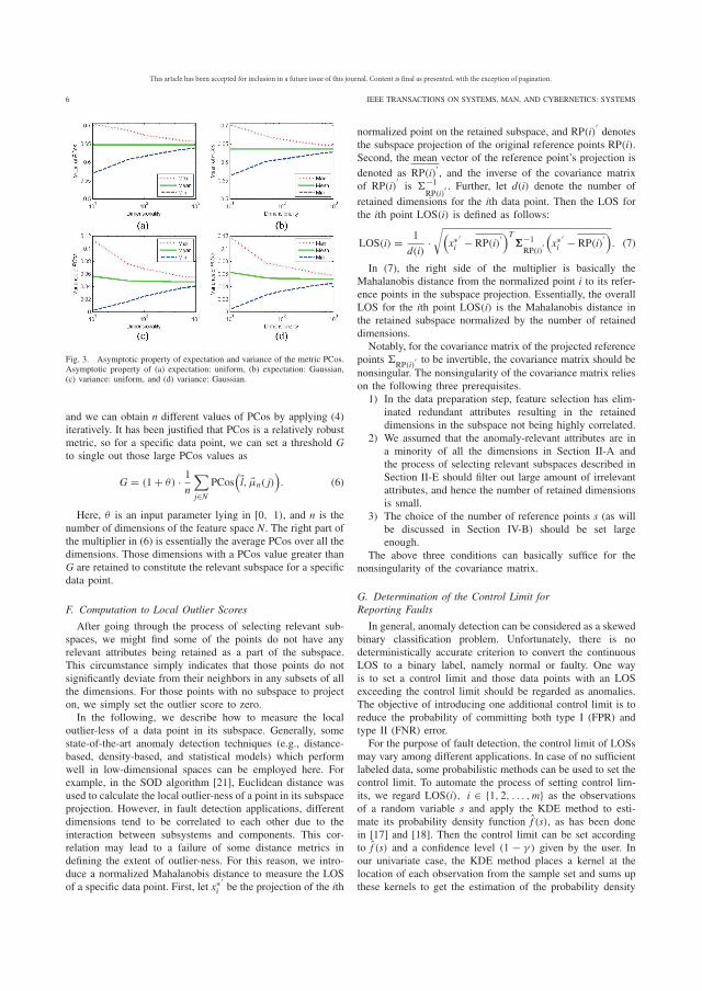
This article has been accepted for inclusion in a future issue of this journal. Content is final as presented, with the exception of pagination.
6 IEEE TRANSACTIONS ON SYSTEMS, MAN, AND CYBERNETICS: SYSTEMS
Fig. 3. Asymptotic property of expectation and variance of the metric PCos.Asymptotic property of (a) expectation: uniform, (b) expectation: Gaussian,(c) variance: uniform, and (d) variance: Gaussian.
and we can obtain n different values of PCos by applying (4)iteratively. It has been justified that PCos is a relatively robustmetric, so for a specific data point, we can set a threshold Gto single out those large PCos values as
G = (1+ θ) · 1n
∑j∈N
PCos(�l, �μn( j)
). (6)
Here, θ is an input parameter lying in [0, 1), and n is thenumber of dimensions of the feature space N. The right part ofthe multiplier in (6) is essentially the average PCos over all thedimensions. Those dimensions with a PCos value greater thanG are retained to constitute the relevant subspace for a specificdata point.
F. Computation to Local Outlier Scores
After going through the process of selecting relevant sub-spaces, we might find some of the points do not have anyrelevant attributes being retained as a part of the subspace.This circumstance simply indicates that those points do notsignificantly deviate from their neighbors in any subsets of allthe dimensions. For those points with no subspace to projecton, we simply set the outlier score to zero.In the following, we describe how to measure the local
outlier-less of a data point in its subspace. Generally, somestate-of-the-art anomaly detection techniques (e.g., distance-based, density-based, and statistical models) which performwell in low-dimensional spaces can be employed here. Forexample, in the SOD algorithm [21], Euclidean distance wasused to calculate the local outlier-ness of a point in its subspaceprojection. However, in fault detection applications, differentdimensions tend to be correlated to each other due to theinteraction between subsystems and components. This cor-relation may lead to a failure of some distance metrics indefining the extent of outlier-ness. For this reason, we intro-duce a normalized Mahalanobis distance to measure the LOSof a specific data point. First, let x∗i
′be the projection of the ith
normalized point on the retained subspace, and RP(i)′denotes
the subspace projection of the original reference points RP(i).Second, the mean vector of the reference point’s projection isdenoted as RP(i)
′, and the inverse of the covariance matrix
of RP(i)′is �−1
RP(i)′ . Further, let d(i) denote the number of
retained dimensions for the ith data point. Then the LOS forthe ith point LOS(i) is defined as follows:
LOS(i) = 1
d(i)·√(
x∗i′ − RP(i)
′)T�−1RP(i)
′(x∗i
′ − RP(i)′)
. (7)
In (7), the right side of the multiplier is basically theMahalanobis distance from the normalized point i to its refer-ence points in the subspace projection. Essentially, the overallLOS for the ith point LOS(i) is the Mahalanobis distance inthe retained subspace normalized by the number of retaineddimensions.Notably, for the covariance matrix of the projected reference
points �RP(i)′ to be invertible, the covariance matrix should be
nonsingular. The nonsingularity of the covariance matrix relieson the following three prerequisites.1) In the data preparation step, feature selection has elim-
inated redundant attributes resulting in the retaineddimensions in the subspace not being highly correlated.
2) We assumed that the anomaly-relevant attributes are ina minority of all the dimensions in Section II-A andthe process of selecting relevant subspaces described inSection II-E should filter out large amount of irrelevantattributes, and hence the number of retained dimensionsis small.
3) The choice of the number of reference points s (as willbe discussed in Section IV-B) should be set largeenough.
The above three conditions can basically suffice for thenonsingularity of the covariance matrix.
G. Determination of the Control Limit forReporting Faults
In general, anomaly detection can be considered as a skewedbinary classification problem. Unfortunately, there is nodeterministically accurate criterion to convert the continuousLOS to a binary label, namely normal or faulty. One wayis to set a control limit and those data points with an LOSexceeding the control limit should be regarded as anomalies.The objective of introducing one additional control limit is toreduce the probability of committing both type I (FPR) andtype II (FNR) error.For the purpose of fault detection, the control limit of LOSs
may vary among different applications. In case of no sufficientlabeled data, some probabilistic methods can be used to set thecontrol limit. To automate the process of setting control lim-its, we regard LOS(i), i ∈ {1, 2, . . . ,m} as the observationsof a random variable s and apply the KDE method to esti-mate its probability density function f (s), as has been donein [17] and [18]. Then the control limit can be set accordingto f (s) and a confidence level (1 − γ ) given by the user. Inour univariate case, the KDE method places a kernel at thelocation of each observation from the sample set and sums upthese kernels to get the estimation of the probability density
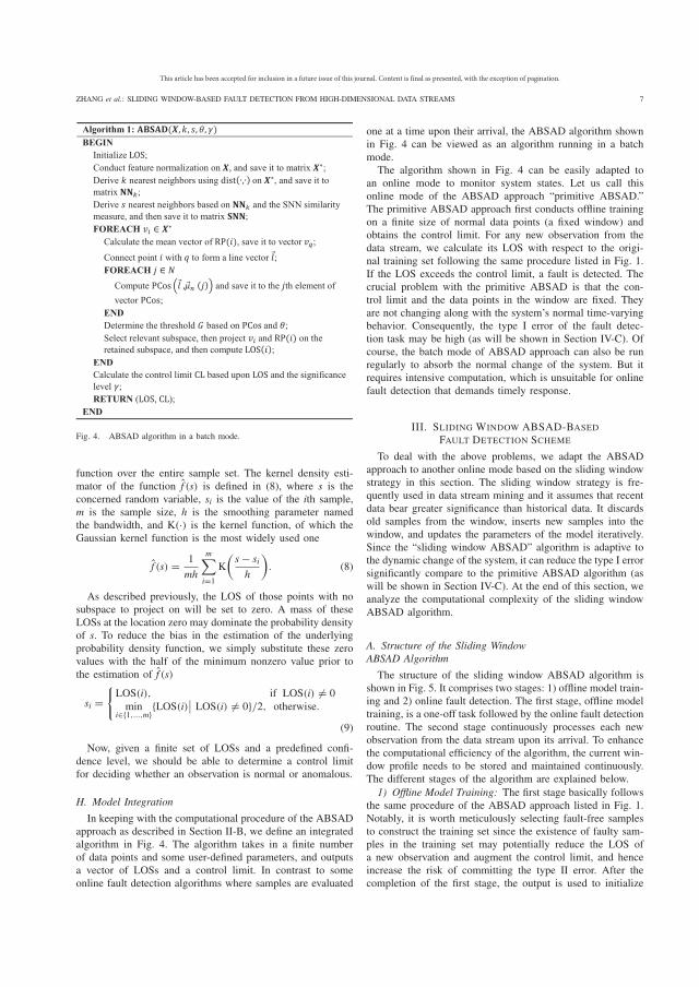
This article has been accepted for inclusion in a future issue of this journal. Content is final as presented, with the exception of pagination.
ZHANG et al.: SLIDING WINDOW-BASED FAULT DETECTION FROM HIGH-DIMENSIONAL DATA STREAMS 7
Fig. 4. ABSAD algorithm in a batch mode.
function over the entire sample set. The kernel density esti-mator of the function f (s) is defined in (8), where s is theconcerned random variable, si is the value of the ith sample,m is the sample size, h is the smoothing parameter namedthe bandwidth, and K(·) is the kernel function, of which theGaussian kernel function is the most widely used one
f (s) = 1
mh
m∑i=1
K
(s − sih
). (8)
As described previously, the LOS of those points with nosubspace to project on will be set to zero. A mass of theseLOSs at the location zero may dominate the probability densityof s. To reduce the bias in the estimation of the underlyingprobability density function, we simply substitute these zerovalues with the half of the minimum nonzero value prior tothe estimation of f (s)
si ={LOS(i), if LOS(i) = 0min
i∈{1,...,m}{LOS(i)∣∣ LOS(i) = 0}/2, otherwise.
(9)
Now, given a finite set of LOSs and a predefined confi-dence level, we should be able to determine a control limitfor deciding whether an observation is normal or anomalous.
H. Model Integration
In keeping with the computational procedure of the ABSADapproach as described in Section II-B, we define an integratedalgorithm in Fig. 4. The algorithm takes in a finite numberof data points and some user-defined parameters, and outputsa vector of LOSs and a control limit. In contrast to someonline fault detection algorithms where samples are evaluated
one at a time upon their arrival, the ABSAD algorithm shownin Fig. 4 can be viewed as an algorithm running in a batchmode.The algorithm shown in Fig. 4 can be easily adapted to
an online mode to monitor system states. Let us call thisonline mode of the ABSAD approach “primitive ABSAD.”The primitive ABSAD approach first conducts offline trainingon a finite size of normal data points (a fixed window) andobtains the control limit. For any new observation from thedata stream, we calculate its LOS with respect to the origi-nal training set following the same procedure listed in Fig. 1.If the LOS exceeds the control limit, a fault is detected. Thecrucial problem with the primitive ABSAD is that the con-trol limit and the data points in the window are fixed. Theyare not changing along with the system’s normal time-varyingbehavior. Consequently, the type I error of the fault detec-tion task may be high (as will be shown in Section IV-C). Ofcourse, the batch mode of ABSAD approach can also be runregularly to absorb the normal change of the system. But itrequires intensive computation, which is unsuitable for onlinefault detection that demands timely response.
III. SLIDING WINDOW ABSAD-BASEDFAULT DETECTION SCHEME
To deal with the above problems, we adapt the ABSADapproach to another online mode based on the sliding windowstrategy in this section. The sliding window strategy is fre-quently used in data stream mining and it assumes that recentdata bear greater significance than historical data. It discardsold samples from the window, inserts new samples into thewindow, and updates the parameters of the model iteratively.Since the “sliding window ABSAD” algorithm is adaptive tothe dynamic change of the system, it can reduce the type I errorsignificantly compare to the primitive ABSAD algorithm (aswill be shown in Section IV-C). At the end of this section, weanalyze the computational complexity of the sliding windowABSAD algorithm.
A. Structure of the Sliding WindowABSAD Algorithm
The structure of the sliding window ABSAD algorithm isshown in Fig. 5. It comprises two stages: 1) offline model train-ing and 2) online fault detection. The first stage, offline modeltraining, is a one-off task followed by the online fault detectionroutine. The second stage continuously processes each newobservation from the data stream upon its arrival. To enhancethe computational efficiency of the algorithm, the current win-dow profile needs to be stored and maintained continuously.The different stages of the algorithm are explained below.1) Offline Model Training: The first stage basically follows
the same procedure of the ABSAD approach listed in Fig. 1.Notably, it is worth meticulously selecting fault-free samplesto construct the training set since the existence of faulty sam-ples in the training set may potentially reduce the LOS ofa new observation and augment the control limit, and henceincrease the risk of committing the type II error. After thecompletion of the first stage, the output is used to initialize

This article has been accepted for inclusion in a future issue of this journal. Content is final as presented, with the exception of pagination.
8 IEEE TRANSACTIONS ON SYSTEMS, MAN, AND CYBERNETICS: SYSTEMS
Fig. 5. Structure of the sliding window ABSAD algorithm.
the profile of the first window. Then, the algorithm is preparedfor the succeeding online fault detection routine.2) Online Fault Detection: The second stage continuously
processes the data stream and monitors the states of thesystem. In accordance with the flow chart of the onlinefault detection stage shown in Fig. 5, the concrete steps areexplained as follows. First, the first two steps, sampling anddata preprocessing, collect the raw data and transform it intoa required form that is appropriate for mining. Specifically,the sampling step acquires real-time measurements in a rawformat. Then the data preprocessing step transforms the rawdata into a suitable format which is in line with the outputformat of the data preparation step in the first stage. Second,the subsequent four steps calculate the local outlier-ness ofa new sample. They again align with the steps listed in Fig. 1.The difference is that there is only one observation goingthrough these steps at a time in order to be processed. Inaddition, the information stored in the current window profileshould be utilized in these two steps: 1) feature normaliza-tion and 2) derivation of the reference set, as indicated bythe dashed arrow in Fig. 5. Concretely, according to (1), thefeature normalization step standardizes the new sample basedon the mean vector and the standard deviation vector storedin the current window profile. In addition, the reference set ofthe new sample originates from the most recent normal sam-ples maintained in the current window profile. Calculating theSNNs of a coming online sample with respect to all the sam-ples in the current window profile yields its reference points.According to (2), the KNN list in the window profile canalso speed up the derivation of the reference set of the newsample. After going through the same process described inSections II-E and II-F, the LOS of the new sample can becalculated. Lastly, we may regard the remaining parts of thesecond stage as the post-processing steps. On the one hand, ifthe obtained LOS exceeds the control limit in the current win-dow profile, a possible fault is then detected and the processstarts over from the resampling step. Meanwhile, if severalconsecutive faults are detected, an alarm should be triggered.
Fig. 6. Transition of the window profile.
In this case, the window profile should not be updated. On theother hand, if the LOS is less or equal than the control limit,the current window profile should be updated to incorporatethe normal change of the system and then the process goesback to the resampling step.In the above algorithm, the first stage learns the normal
behavior of the monitored system and stores the key infor-mation into the first window. The second stage continuouslydetects whether a new sample is normal or faulty based onthe information preserved in the current window profile. Ifa new sample is judged to be normal, the information con-tained in this sample will be absorbed into the new window.Correspondingly, the information of the oldest sample will bediscarded. By doing so, the latest normal behavior of the sys-tem can always be incorporated into the current window andserves as the basis for dynamic fault detection. Among allthe steps in the sliding window ABSAD algorithm, updatingthe window profile is the most critical and complex one. Theupdating mechanism will be elaborated in the next section.
B. Update to the Current Window Profile
Through updating the current window profile regularly, thesliding window strategy enables the online fault detection toadapt to the time-varying behavior of the system. Based onthe requirements of the ABSAD approach, six items are iden-tified to be preserved and maintained in the window profile,i.e., samples, mean vector, standard deviation vector, KNN list,k-distance vector, and the control limit, as shown in Fig. 6.The following contents will mainly discuss how to updatethese items.Before looking at the details, let us make some more nota-
tions. We define W(i) as all the samples in the ith windowwith a window size L. As shown in Fig. 6, W(i) is a L byn matrix, in which each row represents one sample (e.g., xiis the first sample in the ith window) and n is the numberof dimensions in the feature space. Notably, the window pro-file is updated only under the condition that a new sampleis judged to be normal. Therefore, the samples preserved ina window may not be consecutive in the time scale even thoughthe samples in a window are sequentially indexed. Further, letx(i), σ (i), kNN-list(i), k-Dist(i), and CL(i) be the columnwisemean vector, columnwise standard deviation vector, KNN list(a set of sets, containing the k nearest neighbors of every sam-ple in the ith window), k-distance vector, and the control limitof the ith window correspondingly. The initialization to thefirst window after the offline model training stage is ratherstraightforward. Now we elaborate the updating mechanismto the six items of the window profile from the ith window tothe (i+ 1)th window as below.
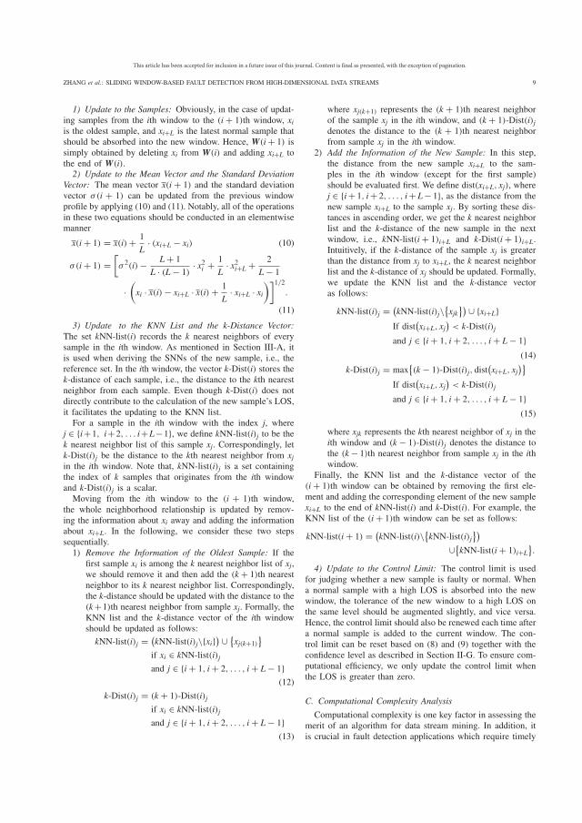
This article has been accepted for inclusion in a future issue of this journal. Content is final as presented, with the exception of pagination.
ZHANG et al.: SLIDING WINDOW-BASED FAULT DETECTION FROM HIGH-DIMENSIONAL DATA STREAMS 9
1) Update to the Samples: Obviously, in the case of updat-ing samples from the ith window to the (i + 1)th window, xiis the oldest sample, and xi+L is the latest normal sample thatshould be absorbed into the new window. Hence, W(i+ 1) issimply obtained by deleting xi from W(i) and adding xi+L tothe end of W(i).2) Update to the Mean Vector and the Standard Deviation
Vector: The mean vector x(i + 1) and the standard deviationvector σ(i + 1) can be updated from the previous windowprofile by applying (10) and (11). Notably, all of the operationsin these two equations should be conducted in an elementwisemanner
x(i + 1) = x(i) + 1
L· (xi+L − xi) (10)
σ(i + 1) =[σ 2(i) − L + 1
L · (L − 1)· x2i + 1
L· x2i+L + 2
L − 1
·(xi · x(i) − xi+L · x(i) + 1
L· xi+L · xi
)]1/2.
(11)
3) Update to the KNN List and the k-Distance Vector:The set kNN-list(i) records the k nearest neighbors of everysample in the ith window. As mentioned in Section III-A, itis used when deriving the SNNs of the new sample, i.e., thereference set. In the ith window, the vector k-Dist(i) stores thek-distance of each sample, i.e., the distance to the kth nearestneighbor from each sample. Even though k-Dist(i) does notdirectly contribute to the calculation of the new sample’s LOS,it facilitates the updating to the KNN list.For a sample in the ith window with the index j, where
j ∈ {i+1, i+2, . . . i+L−1}, we define kNN-list(i)j to be thek nearest neighbor list of this sample xj. Correspondingly, letk-Dist(i)j be the distance to the kth nearest neighbor from xjin the ith window. Note that, kNN-list(i)j is a set containingthe index of k samples that originates from the ith windowand k-Dist(i)j is a scalar.Moving from the ith window to the (i + 1)th window,
the whole neighborhood relationship is updated by remov-ing the information about xi away and adding the informationabout xi+L. In the following, we consider these two stepssequentially.1) Remove the Information of the Oldest Sample: If the
first sample xi is among the k nearest neighbor list of xj,we should remove it and then add the (k+ 1)th nearestneighbor to its k nearest neighbor list. Correspondingly,the k-distance should be updated with the distance to the(k+1)th nearest neighbor from sample xj. Formally, theKNN list and the k-distance vector of the ith windowshould be updated as follows:
kNN-list(i)j = (kNN-list(i)j\{xi}
) ∪ {xj(k+1)
}if xi ∈ kNN-list(i)jand j ∈ {i+ 1, i + 2, . . . , i + L − 1}
(12)
k-Dist(i)j = (k + 1)-Dist(i)jif xi ∈ kNN-list(i)jand j ∈ {i+ 1, i + 2, . . . , i + L − 1}
(13)
where xj(k+1) represents the (k + 1)th nearest neighborof the sample xj in the ith window, and (k + 1)-Dist(i)jdenotes the distance to the (k + 1)th nearest neighborfrom sample xj in the ith window.
2) Add the Information of the New Sample: In this step,the distance from the new sample xi+L to the sam-ples in the ith window (except for the first sample)should be evaluated first. We define dist(xi+L, xj), wherej ∈ {i+ 1, i+ 2, . . . , i+ L− 1}, as the distance from thenew sample xi+L to the sample xj. By sorting these dis-tances in ascending order, we get the k nearest neighborlist and the k-distance of the new sample in the nextwindow, i.e., kNN-list(i+ 1)i+L and k-Dist(i + 1)i+L.Intuitively, if the k-distance of the sample xj is greaterthan the distance from xj to xi+L, the k nearest neighborlist and the k-distance of xj should be updated. Formally,we update the KNN list and the k-distance vectoras follows:
kNN-list(i)j = (kNN-list(i)j\
{xjk
}) ∪ {xi+L}If dist
(xi+L, xj
)< k-Dist(i)j
and j ∈ {i+ 1, i + 2, . . . , i + L − 1}(14)
k-Dist(i)j = max{(k − 1)-Dist(i)j, dist
(xi+L, xj
)}If dist
(xi+L, xj
)< k-Dist(i)j
and j ∈ {i+ 1, i + 2, . . . , i + L − 1}(15)
where xjk represents the kth nearest neighbor of xj in theith window and (k − 1)-Dist(i)j denotes the distance tothe (k− 1)th nearest neighbor from sample xj in the ithwindow.
Finally, the KNN list and the k-distance vector of the(i+ 1)th window can be obtained by removing the first ele-ment and adding the corresponding element of the new samplexi+L to the end of kNN-list(i) and k-Dist(i). For example, theKNN list of the (i+ 1)th window can be set as follows:
kNN-list(i + 1) = (kNN-list(i)\{kNN-list(i)j})
∪{kNN-list(i+ 1)i+L
}.
4) Update to the Control Limit: The control limit is usedfor judging whether a new sample is faulty or normal. Whena normal sample with a high LOS is absorbed into the newwindow, the tolerance of the new window to a high LOS onthe same level should be augmented slightly, and vice versa.Hence, the control limit should also be renewed each time aftera normal sample is added to the current window. The con-trol limit can be reset based on (8) and (9) together with theconfidence level as described in Section II-G. To ensure com-putational efficiency, we only update the control limit whenthe LOS is greater than zero.
C. Computational Complexity Analysis
Computational complexity is one key factor in assessing themerit of an algorithm for data stream mining. In addition, itis crucial in fault detection applications which require timely
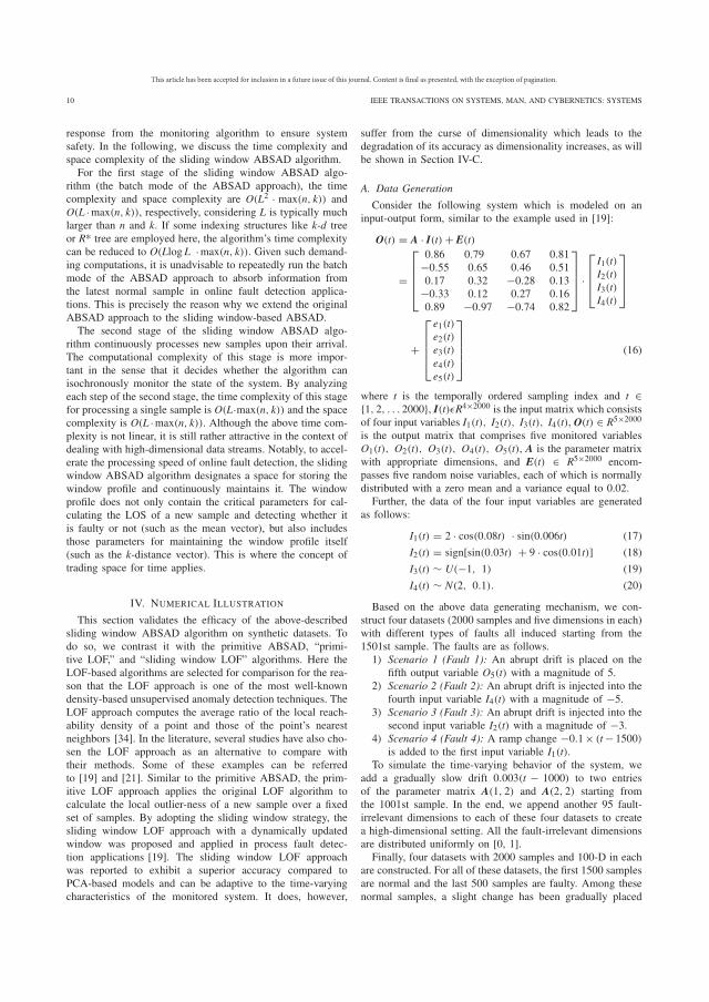
This article has been accepted for inclusion in a future issue of this journal. Content is final as presented, with the exception of pagination.
10 IEEE TRANSACTIONS ON SYSTEMS, MAN, AND CYBERNETICS: SYSTEMS
response from the monitoring algorithm to ensure systemsafety. In the following, we discuss the time complexity andspace complexity of the sliding window ABSAD algorithm.For the first stage of the sliding window ABSAD algo-
rithm (the batch mode of the ABSAD approach), the timecomplexity and space complexity are O(L2 · max(n, k)) andO(L ·max(n, k)), respectively, considering L is typically muchlarger than n and k. If some indexing structures like k-d treeor R* tree are employed here, the algorithm’s time complexitycan be reduced to O(Llog L ·max(n, k)). Given such demand-ing computations, it is unadvisable to repeatedly run the batchmode of the ABSAD approach to absorb information fromthe latest normal sample in online fault detection applica-tions. This is precisely the reason why we extend the originalABSAD approach to the sliding window-based ABSAD.The second stage of the sliding window ABSAD algo-
rithm continuously processes new samples upon their arrival.The computational complexity of this stage is more impor-tant in the sense that it decides whether the algorithm canisochronously monitor the state of the system. By analyzingeach step of the second stage, the time complexity of this stagefor processing a single sample is O(L·max(n, k)) and the spacecomplexity is O(L ·max(n, k)). Although the above time com-plexity is not linear, it is still rather attractive in the context ofdealing with high-dimensional data streams. Notably, to accel-erate the processing speed of online fault detection, the slidingwindow ABSAD algorithm designates a space for storing thewindow profile and continuously maintains it. The windowprofile does not only contain the critical parameters for cal-culating the LOS of a new sample and detecting whether itis faulty or not (such as the mean vector), but also includesthose parameters for maintaining the window profile itself(such as the k-distance vector). This is where the concept oftrading space for time applies.
IV. NUMERICAL ILLUSTRATION
This section validates the efficacy of the above-describedsliding window ABSAD algorithm on synthetic datasets. Todo so, we contrast it with the primitive ABSAD, “primi-tive LOF,” and “sliding window LOF” algorithms. Here theLOF-based algorithms are selected for comparison for the rea-son that the LOF approach is one of the most well-knowndensity-based unsupervised anomaly detection techniques. TheLOF approach computes the average ratio of the local reach-ability density of a point and those of the point’s nearestneighbors [34]. In the literature, several studies have also cho-sen the LOF approach as an alternative to compare withtheir methods. Some of these examples can be referredto [19] and [21]. Similar to the primitive ABSAD, the prim-itive LOF approach applies the original LOF algorithm tocalculate the local outlier-ness of a new sample over a fixedset of samples. By adopting the sliding window strategy, thesliding window LOF approach with a dynamically updatedwindow was proposed and applied in process fault detec-tion applications [19]. The sliding window LOF approachwas reported to exhibit a superior accuracy compared toPCA-based models and can be adaptive to the time-varyingcharacteristics of the monitored system. It does, however,
suffer from the curse of dimensionality which leads to thedegradation of its accuracy as dimensionality increases, as willbe shown in Section IV-C.
A. Data Generation
Consider the following system which is modeled on aninput-output form, similar to the example used in [19]:
O(t) = A · I(t) + E(t)
=
⎡⎢⎢⎢⎣
0.86 0.79 0.67 0.81−0.55 0.65 0.46 0.510.17 0.32 −0.28 0.13
−0.33 0.12 0.27 0.160.89 −0.97 −0.74 0.82
⎤⎥⎥⎥⎦ ·
⎡⎢⎢⎣I1(t)I2(t)I3(t)I4(t)
⎤⎥⎥⎦
+
⎡⎢⎢⎢⎣e1(t)e2(t)e3(t)e4(t)e5(t)
⎤⎥⎥⎥⎦ (16)
where t is the temporally ordered sampling index and t ∈{1, 2, . . . 2000}, I(t)εR4×2000 is the input matrix which consistsof four input variables I1(t), I2(t), I3(t), I4(t), O(t) ∈ R5×2000is the output matrix that comprises five monitored variablesO1(t), O2(t), O3(t), O4(t), O5(t), A is the parameter matrixwith appropriate dimensions, and E(t) ∈ R5×2000 encom-passes five random noise variables, each of which is normallydistributed with a zero mean and a variance equal to 0.02.Further, the data of the four input variables are generated
as follows:
I1(t) = 2 · cos(0.08t) · sin(0.006t) (17)
I2(t) = sign[sin(0.03t) + 9 · cos(0.01t)] (18)
I3(t) ∼ U(−1, 1) (19)
I4(t) ∼ N(2, 0.1). (20)
Based on the above data generating mechanism, we con-struct four datasets (2000 samples and five dimensions in each)with different types of faults all induced starting from the1501st sample. The faults are as follows.1) Scenario 1 (Fault 1): An abrupt drift is placed on the
fifth output variable O5(t) with a magnitude of 5.2) Scenario 2 (Fault 2): An abrupt drift is injected into the
fourth input variable I4(t) with a magnitude of −5.3) Scenario 3 (Fault 3): An abrupt drift is injected into the
second input variable I2(t) with a magnitude of −3.4) Scenario 4 (Fault 4): A ramp change −0.1× (t− 1500)
is added to the first input variable I1(t).To simulate the time-varying behavior of the system, we
add a gradually slow drift 0.003(t − 1000) to two entriesof the parameter matrix A(1, 2) and A(2, 2) starting fromthe 1001st sample. In the end, we append another 95 fault-irrelevant dimensions to each of these four datasets to createa high-dimensional setting. All the fault-irrelevant dimensionsare distributed uniformly on [0, 1].Finally, four datasets with 2000 samples and 100-D in each
are constructed. For all of these datasets, the first 1500 samplesare normal and the last 500 samples are faulty. Among thesenormal samples, a slight change has been gradually placed
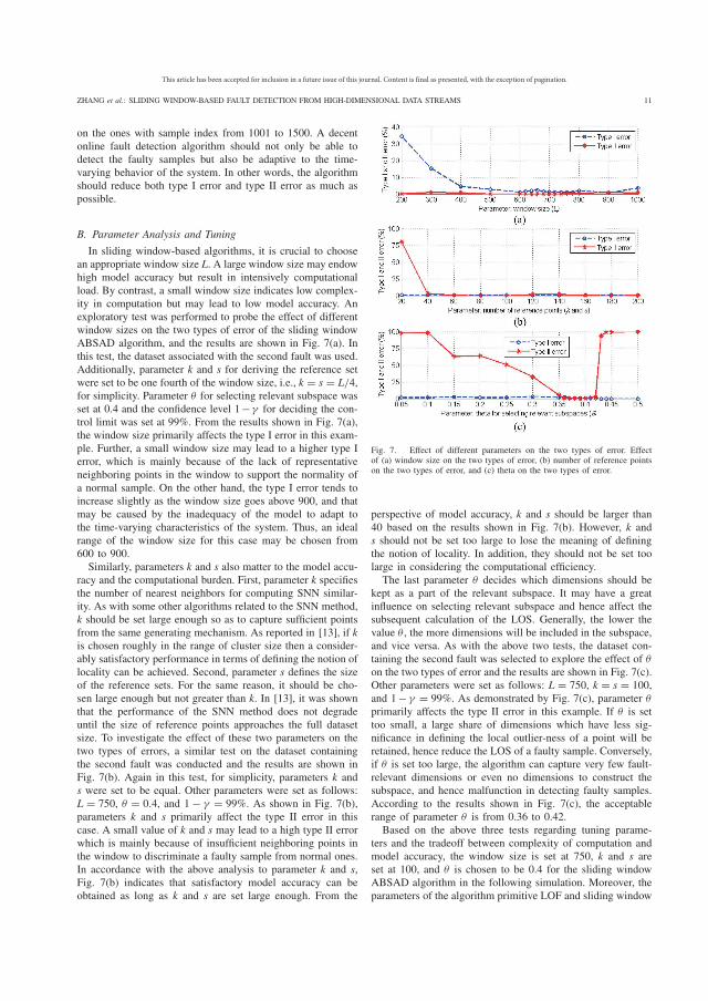
This article has been accepted for inclusion in a future issue of this journal. Content is final as presented, with the exception of pagination.
ZHANG et al.: SLIDING WINDOW-BASED FAULT DETECTION FROM HIGH-DIMENSIONAL DATA STREAMS 11
on the ones with sample index from 1001 to 1500. A decentonline fault detection algorithm should not only be able todetect the faulty samples but also be adaptive to the time-varying behavior of the system. In other words, the algorithmshould reduce both type I error and type II error as much aspossible.
B. Parameter Analysis and Tuning
In sliding window-based algorithms, it is crucial to choosean appropriate window size L. A large window size may endowhigh model accuracy but result in intensively computationalload. By contrast, a small window size indicates low complex-ity in computation but may lead to low model accuracy. Anexploratory test was performed to probe the effect of differentwindow sizes on the two types of error of the sliding windowABSAD algorithm, and the results are shown in Fig. 7(a). Inthis test, the dataset associated with the second fault was used.Additionally, parameter k and s for deriving the reference setwere set to be one fourth of the window size, i.e., k = s = L/4,for simplicity. Parameter θ for selecting relevant subspace wasset at 0.4 and the confidence level 1−γ for deciding the con-trol limit was set at 99%. From the results shown in Fig. 7(a),the window size primarily affects the type I error in this exam-ple. Further, a small window size may lead to a higher type Ierror, which is mainly because of the lack of representativeneighboring points in the window to support the normality ofa normal sample. On the other hand, the type I error tends toincrease slightly as the window size goes above 900, and thatmay be caused by the inadequacy of the model to adapt tothe time-varying characteristics of the system. Thus, an idealrange of the window size for this case may be chosen from600 to 900.Similarly, parameters k and s also matter to the model accu-
racy and the computational burden. First, parameter k specifiesthe number of nearest neighbors for computing SNN similar-ity. As with some other algorithms related to the SNN method,k should be set large enough so as to capture sufficient pointsfrom the same generating mechanism. As reported in [13], if kis chosen roughly in the range of cluster size then a consider-ably satisfactory performance in terms of defining the notion oflocality can be achieved. Second, parameter s defines the sizeof the reference sets. For the same reason, it should be cho-sen large enough but not greater than k. In [13], it was shownthat the performance of the SNN method does not degradeuntil the size of reference points approaches the full datasetsize. To investigate the effect of these two parameters on thetwo types of errors, a similar test on the dataset containingthe second fault was conducted and the results are shown inFig. 7(b). Again in this test, for simplicity, parameters k ands were set to be equal. Other parameters were set as follows:L = 750, θ = 0.4, and 1− γ = 99%. As shown in Fig. 7(b),parameters k and s primarily affect the type II error in thiscase. A small value of k and s may lead to a high type II errorwhich is mainly because of insufficient neighboring points inthe window to discriminate a faulty sample from normal ones.In accordance with the above analysis to parameter k and s,Fig. 7(b) indicates that satisfactory model accuracy can beobtained as long as k and s are set large enough. From the
Fig. 7. Effect of different parameters on the two types of error. Effectof (a) window size on the two types of error, (b) number of reference pointson the two types of error, and (c) theta on the two types of error.
perspective of model accuracy, k and s should be larger than40 based on the results shown in Fig. 7(b). However, k ands should not be set too large to lose the meaning of definingthe notion of locality. In addition, they should not be set toolarge in considering the computational efficiency.The last parameter θ decides which dimensions should be
kept as a part of the relevant subspace. It may have a greatinfluence on selecting relevant subspace and hence affect thesubsequent calculation of the LOS. Generally, the lower thevalue θ , the more dimensions will be included in the subspace,and vice versa. As with the above two tests, the dataset con-taining the second fault was selected to explore the effect of θ
on the two types of error and the results are shown in Fig. 7(c).Other parameters were set as follows: L = 750, k = s = 100,and 1− γ = 99%. As demonstrated by Fig. 7(c), parameter θ
primarily affects the type II error in this example. If θ is settoo small, a large share of dimensions which have less sig-nificance in defining the local outlier-ness of a point will beretained, hence reduce the LOS of a faulty sample. Conversely,if θ is set too large, the algorithm can capture very few fault-relevant dimensions or even no dimensions to construct thesubspace, and hence malfunction in detecting faulty samples.According to the results shown in Fig. 7(c), the acceptablerange of parameter θ is from 0.36 to 0.42.Based on the above three tests regarding tuning parame-
ters and the tradeoff between complexity of computation andmodel accuracy, the window size is set at 750, k and s areset at 100, and θ is chosen to be 0.4 for the sliding windowABSAD algorithm in the following simulation. Moreover, theparameters of the algorithm primitive LOF and sliding window
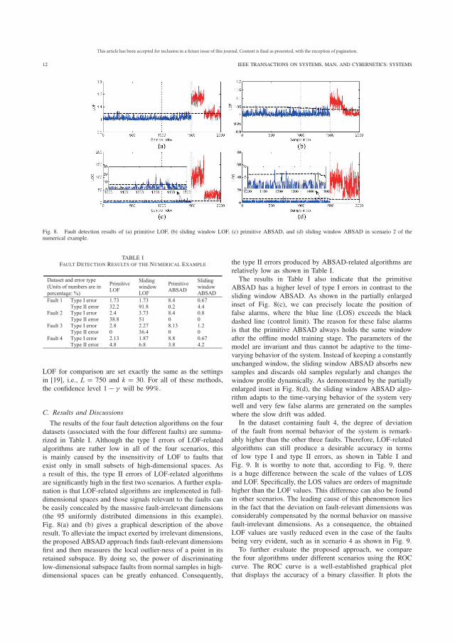
This article has been accepted for inclusion in a future issue of this journal. Content is final as presented, with the exception of pagination.
12 IEEE TRANSACTIONS ON SYSTEMS, MAN, AND CYBERNETICS: SYSTEMS
Fig. 8. Fault detection results of (a) primitive LOF, (b) sliding window LOF, (c) primitive ABSAD, and (d) sliding window ABSAD in scenario 2 of thenumerical example.
TABLE IFAULT DETECTION RESULTS OF THE NUMERICAL EXAMPLE
LOF for comparison are set exactly the same as the settingsin [19], i.e., L = 750 and k = 30. For all of these methods,the confidence level 1− γ will be 99%.
C. Results and Discussions
The results of the four fault detection algorithms on the fourdatasets (associated with the four different faults) are summa-rized in Table I. Although the type I errors of LOF-relatedalgorithms are rather low in all of the four scenarios, thisis mainly caused by the insensitivity of LOF to faults thatexist only in small subsets of high-dimensional spaces. Asa result of this, the type II errors of LOF-related algorithmsare significantly high in the first two scenarios. A further expla-nation is that LOF-related algorithms are implemented in full-dimensional spaces and those signals relevant to the faults canbe easily concealed by the massive fault-irrelevant dimensions(the 95 uniformly distributed dimensions in this example).Fig. 8(a) and (b) gives a graphical description of the aboveresult. To alleviate the impact exerted by irrelevant dimensions,the proposed ABSAD approach finds fault-relevant dimensionsfirst and then measures the local outlier-ness of a point in itsretained subspace. By doing so, the power of discriminatinglow-dimensional subspace faults from normal samples in high-dimensional spaces can be greatly enhanced. Consequently,
the type II errors produced by ABSAD-related algorithms arerelatively low as shown in Table I.The results in Table I also indicate that the primitive
ABSAD has a higher level of type I errors in contrast to thesliding window ABSAD. As shown in the partially enlargedinset of Fig. 8(c), we can precisely locate the position offalse alarms, where the blue line (LOS) exceeds the blackdashed line (control limit). The reason for these false alarmsis that the primitive ABSAD always holds the same windowafter the offline model training stage. The parameters of themodel are invariant and thus cannot be adaptive to the time-varying behavior of the system. Instead of keeping a constantlyunchanged window, the sliding window ABSAD absorbs newsamples and discards old samples regularly and changes thewindow profile dynamically. As demonstrated by the partiallyenlarged inset in Fig. 8(d), the sliding window ABSAD algo-rithm adapts to the time-varying behavior of the system verywell and very few false alarms are generated on the sampleswhere the slow drift was added.In the dataset containing fault 4, the degree of deviation
of the fault from normal behavior of the system is remark-ably higher than the other three faults. Therefore, LOF-relatedalgorithms can still produce a desirable accuracy in termsof low type I and type II errors, as shown in Table I andFig. 9. It is worthy to note that, according to Fig. 9, thereis a huge difference between the scale of the values of LOSand LOF. Specifically, the LOS values are orders of magnitudehigher than the LOF values. This difference can also be foundin other scenarios. The leading cause of this phenomenon liesin the fact that the deviation on fault-relevant dimensions wasconsiderably compensated by the normal behavior on massivefault-irrelevant dimensions. As a consequence, the obtainedLOF values are vastly reduced even in the case of the faultsbeing very evident, such as in scenario 4 as shown in Fig. 9.To further evaluate the proposed approach, we compare
the four algorithms under different scenarios using the ROCcurve. The ROC curve is a well-established graphical plotthat displays the accuracy of a binary classifier. It plots the

This article has been accepted for inclusion in a future issue of this journal. Content is final as presented, with the exception of pagination.
ZHANG et al.: SLIDING WINDOW-BASED FAULT DETECTION FROM HIGH-DIMENSIONAL DATA STREAMS 13
Fig. 9. Fault detection results of (a) primitive LOF, (b) sliding window LOF, (c) primitive ABSAD, and (d) sliding window ABSAD in scenario 4 of thenumerical example.
Fig. 10. ROC curve of the four algorithms under different faulty scenarios.(a) Scenario 1. (b) Scenario 2. (c) Scenario 3. (d) Scenario 4.
TPR against the FPR at various threshold settings, i.e., thresh-old independent. The larger the AUC, the better accuracya binary classifier can achieve. As expected, the results shownin Fig. 10 again demonstrate the superior accuracy of ABSAD-related algorithms over LOF-related algorithms. Notably, it isdifficult to tell the difference between the ROC curve of thesliding window ABSAD and the primitive ABSAD in theseplots. We would consider this as another evidence to show thenecessity of introducing the updating mechanism to the controllimit as suggested in the sliding window ABSAD algorithm.The presence of measurement noises or disturbances may
lead to either false alarms or missed detections. As dis-cussed in [4], a reasonable fault detection algorithm shouldbe sensitive to faults, as well as robust against measure-ment noises or disturbances. The proposed ABSAD approach
defines a threshold using (6) to single out those dimensionsin which faulty signals may exist. On the other hand, it fil-ters those dimensions that are less likely to be faulty, andthereby dimension-wisely attenuating the effect of measure-ment noises and of the disturbances. Moreover, the controllimit defined in the sliding window ABSAD algorithm servesas a way to sample-wisely attenuate disturbance and noisesignals. By adaptively updating the control limit, the onlinealgorithm provides a better noise and disturbance attenuationability over nonstationary systems.The accuracy of those algorithms implemented on full-
dimensional spaces, such as LOF, degrades significantly asdimensionality increases. To mitigate the influence exertedby irrelevant dimensions, the ABSAD approach computes thedegree of deviation of a data point on its derived subspaceprojection. As we claimed in Section II, the retained subspaceshould be meaningful in the sense that it should be able tocapture most of the information with regard to the discordanceof an object to its adjacent data instances. By examining theretained subspace of the faults in all the four scenarios, wefound that the dimensions in the subspace are exactly the sameposition where the faults were induced on.Execution speed is another significant performance indicator
of an algorithm, especially to those online algorithms dealingwith high-speed data streams. Although the sliding win-dow ABSAD algorithm is more computationally demandingthan the LOF-based algorithms as shown by our experi-ments, it is still attractive in the context of high-dimensionaldata streams based on our computational complexity analy-sis in Section III-C. As mentioned earlier, trading space fortime is one strategy for our online algorithm to speed up thecomputation and the other one is the use of some indexingstructures. Notably, the computation of the ABSAD approachwithin each step does not need to be sequentially executed. Forexample, when deriving the reference set of a new sample, thedistance from this sample to other samples in the current win-dow profile can be calculated concurrently. This gives us the
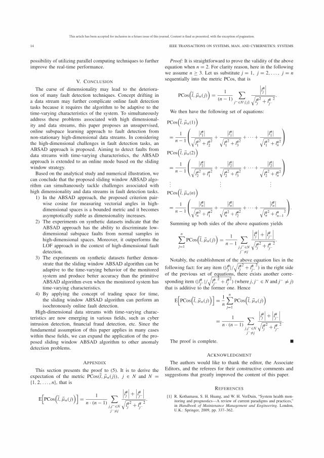
This article has been accepted for inclusion in a future issue of this journal. Content is final as presented, with the exception of pagination.
14 IEEE TRANSACTIONS ON SYSTEMS, MAN, AND CYBERNETICS: SYSTEMS
possibility of utilizing parallel computing techniques to furtherimprove the real-time performance.
V. CONCLUSION
The curse of dimensionality may lead to the deteriora-tion of many fault detection techniques. Concept drifting ina data stream may further complicate online fault detectiontasks because it requires the algorithm to be adaptive to thetime-varying characteristics of the system. To simultaneouslyaddress these problems associated with high dimensional-ity and data streams, this paper proposes an unsupervised,online subspace learning approach to fault detection fromnon-stationary high-dimensional data streams. In consideringthe high-dimensional challenges in fault detection tasks, anABSAD approach is proposed. Aiming to detect faults fromdata streams with time-varying characteristics, the ABSADapproach is extended to an online mode based on the slidingwindow strategy.Based on the analytical study and numerical illustration, we
can conclude that the proposed sliding window ABSAD algo-rithm can simultaneously tackle challenges associated withhigh dimensionality and data streams in fault detection tasks.1) In the ABSAD approach, the proposed criterion pair-
wise cosine for measuring vectorial angles in high-dimensional spaces is a bounded metric and it becomesasymptotically stable as dimensionality increases.
2) The experiments on synthetic datasets indicate that theABSAD approach has the ability to discriminate low-dimensional subspace faults from normal samples inhigh-dimensional spaces. Moreover, it outperforms theLOF approach in the context of high-dimensional faultdetection.
3) The experiments on synthetic datasets further demon-strate that the sliding window ABSAD algorithm can beadaptive to the time-varying behavior of the monitoredsystem and produce better accuracy than the primitiveABSAD algorithm even when the monitored system hastime-varying characteristics.
4) By applying the concept of trading space for time,the sliding window ABSAD algorithm can perform anisochronously online fault detection.
High-dimensional data streams with time-varying charac-teristics are now emerging in various fields, such as cyberintrusion detection, financial fraud detection, etc. Since thefundamental assumption of this paper applies in many caseswithin these fields, we can expand the application of the pro-posed sliding window ABSAD algorithm to other anomalydetection problems.
APPENDIX
This section presents the proof to (5). It is to derive theexpectation of the metric PCos(�l, �μn( j)), j ∈ N and N ={1, 2, . . . , n}, that is
E[PCos
(�l, �μn( j))]
= 1
n · (n− 1)
∑j,j−∈Nj− =j
∣∣∣l#j ∣∣∣ +∣∣∣l#j−
∣∣∣√l#j2 + l#j−
2.
Proof: It is straightforward to prove the validity of the aboveequation when n = 2. For clarity reason, here in the followingwe assume n ≥ 3. Let us substitute j = 1, j = 2, . . . , j = nsequentially into the metric PCos, that is
PCos(�l, �μn( j)
)= 1
(n − 1)
∑j−∈N\{ j}
∣∣∣l#j ∣∣∣√l#j2 + l#j−
2.
We then have the following set of equations:
PCos(�l, �μn(1)
)
= 1
n− 1
⎛⎝ ∣∣l#1∣∣√
l#12 + l#2
2+
∣∣l#1∣∣√l#12 + l#3
2+ · · · +
∣∣l#1∣∣√l#12 + l#n
2
⎞⎠
PCos(�l, �μn(2)
)
= 1
n− 1
⎛⎝ ∣∣l#2∣∣√
l#22 + l#1
2+
∣∣l#2∣∣√l#22 + l#3
2+ · · · +
∣∣l#2∣∣√l#22 + l#n
2
⎞⎠
......
...
PCos(�l, �μn(n)
)
= 1
n− 1
⎛⎝ ∣∣l#n∣∣√
l#n2 + l#1
2+
∣∣l#n∣∣√l#n2 + l#2
2+ · · · +
∣∣l#n∣∣√l#n2 + l#n−1
2
⎞⎠.
Summing up both sides of the above equations yields
n∑j=1
PCos(�l, �μn( j)
)= 1
n− 1
∑j,j−∈Nj− =j
∣∣∣l#j ∣∣∣ +∣∣∣l#j−
∣∣∣√l#j2 + l#j−
2.
Notably, the establishment of the above equation lies in the
following fact: for any item (|l#j |/√l#j2 + l#j−
2) in the right side
of the previous set of equations, there exists another corre-
sponding item (|l#j−|/√l#j−
2 + l#j2) (where j, j− ∈ N and j− = j)
that is additive to the former one. Hence
E[PCos
(�l, �μn( j))]
= 1
n
n∑j=1
PCos(�l, �μn( j)
)
= 1
n · (n− 1)
∑j,j−∈Nj− =j
∣∣∣l#j ∣∣∣ +∣∣∣l#j−
∣∣∣√l#j2 + l#j−
2.
The proof is complete.
ACKNOWLEDGMENT
The authors would like to thank the editor, the AssociateEditors, and the referees for their constructive comments andsuggestions that greatly improved the content of this paper.
REFERENCES
[1] R. Kothamasu, S. H. Huang, and W. H. VerDuin, “System health mon-itoring and prognostics—A review of current paradigms and practices,”in Handbook of Maintenance Management and Engineering. London,U.K.: Springer, 2009, pp. 337–362.
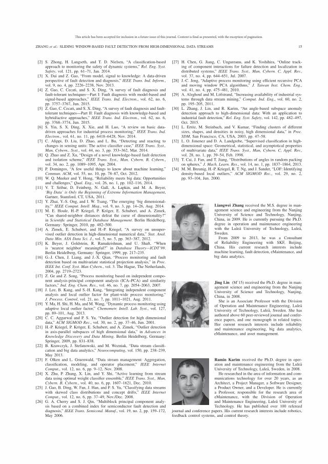
This article has been accepted for inclusion in a future issue of this journal. Content is final as presented, with the exception of pagination.
ZHANG et al.: SLIDING WINDOW-BASED FAULT DETECTION FROM HIGH-DIMENSIONAL DATA STREAMS 15
[2] S. Zhong, H. Langseth, and T. D. Nielsen, “A classification-basedapproach to monitoring the safety of dynamic systems,” Rel. Eng. Syst.Safety, vol. 121, pp. 61–71, Jan. 2014.
[3] X. Dai and Z. Gao, “From model, signal to knowledge: A data-drivenperspective of fault detection and diagnosis,” IEEE Trans. Ind. Inform.,vol. 9, no. 4, pp. 2226–2238, Nov. 2013.
[4] Z. Gao, C. Cecati, and S. X. Ding, “A survey of fault diagnosis andfault-tolerant techniques—Part I: Fault diagnosis with model-based andsignal-based approaches,” IEEE Trans. Ind. Electron., vol. 62, no. 6,pp. 3757–3767, Jun. 2015.
[5] Z. Gao, C. Cecati, and S. X. Ding, “A survey of fault diagnosis and fault-tolerant techniques—Part II: Fault diagnosis with knowledge-based andhybrid/active approaches,” IEEE Trans. Ind. Electron., vol. 62, no. 6,pp. 3768–3774, Jun. 2015.
[6] S. Yin, S. X. Ding, X. Xie, and H. Luo, “A review on basic data-driven approaches for industrial process monitoring,” IEEE Trans. Ind.Electron., vol. 61, no. 11, pp. 6418–6428, Nov. 2014.
[7] C. Alippi, D. Liu, D. Zhao, and L. Bu, “Detecting and reacting tochanges in sensing units: The active classifier case,” IEEE Trans. Syst.,Man, Cybern., Syst., vol. 44, no. 3, pp. 353–362, Mar. 2014.
[8] Q. Zhao and Z. Xu, “Design of a novel knowledge-based fault detectionand isolation scheme,” IEEE Trans. Syst., Man, Cybern. B, Cybern.,vol. 34, no. 2, pp. 1089–1095, Apr. 2004.
[9] P. Domingos, “A few useful things to know about machine learning,”Commun. ACM, vol. 55, no. 10, pp. 78–87, Oct. 2012.
[10] W. Q. Meeker and Y. Hong, “Reliability meets big data: Opportunitiesand challenges,” Qual. Eng., vol. 26, no. 1, pp. 102–116, 2014.
[11] V. T. Sribar, D. Feinberg, N. Gall, A. Lapkin, and M. A. Beyer,‘Big Data’ is Only the Beginning of Extreme Information Management,Gartner, Stamford, CT, USA, 2011.
[12] Y. Zhai, Y.-S. Ong, and I. W. Tsang, “The emerging ‘big dimensional-ity,”’ IEEE Comput. Intell. Mag., vol. 9, no. 3, pp. 14–26, Aug. 2014.
[13] M. E. Houle, H.-P. Kriegel, P. Kröger, E. Schubert, and A. Zimek,“Can shared-neighbor distances defeat the curse of dimensionality?”in Scientific and Statistical Database Management. Berlin Heidelberg,Germany: Springer, 2010, pp. 482–500.
[14] A. Zimek, E. Schubert, and H.-P. Kriegel, “A survey on unsuper-vised outlier detection in high-dimensional numerical data,” Stat. Anal.Data Min. ASA Data Sci. J., vol. 5, no. 5, pp. 363–387, 2012.
[15] K. Beyer, J. Goldstein, R. Ramakrishnan, and U. Shaft, “Whenis ‘nearest neighbor’ meaningful?” in Database Theory—ICDT’99.Berlin Heidelberg, Germany: Springer, 1999, pp. 217–235.
[16] G.-J. Chen, J. Liang, and J.-X. Qian, “Process monitoring and faultdetection based on multivariate statistical projection analysis,” in Proc.IEEE Int. Conf. Syst. Man Cybern., vol. 3. The Hague, The Netherlands,2004, pp. 2719–2723.
[17] Z. Ge and Z. Song, “Process monitoring based on independent compo-nent analysis-principal component analysis (ICA–PCA) and similarityfactors,” Ind. Eng. Chem. Res., vol. 46, no. 7, pp. 2054–2063, 2007.
[18] J. Lee, B. Kang, and S.-H. Kang, “Integrating independent componentanalysis and local outlier factor for plant-wide process monitoring,”J. Process. Control, vol. 21, no. 7, pp. 1011–1021, Aug. 2011.
[19] Y. Ma, H. Shi, H. Ma, and M. Wang, “Dynamic process monitoring usingadaptive local outlier factor,” Chemometr. Intell. Lab. Syst., vol. 127,pp. 89–101, Aug. 2013.
[20] C. C. Aggarwal and P. S. Yu, “Outlier detection for high dimensionaldata,” ACM SIGMOD Rec., vol. 30, no. 2, pp. 37–46, Jun. 2001.
[21] H.-P. Kriegel, P. Kröger, E. Schubert, and A. Zimek, “Outlier detectionin axis-parallel subspaces of high dimensional data,” in Advances inKnowledge Discovery and Data Mining. Berlin Heidelberg, Germany:Springer, 2009, pp. 831–838.
[22] B. Krawczyk, J. Stefanowski, and M. Wozniak, “Data stream classifi-cation and big data analytics,” Neurocomputing, vol. 150, pp. 238–239,May 2013.
[23] F. Olken and L. Gruenwald, “Data stream management: Aggregation,classification, modeling, and operator placement,” IEEE InternetComput., vol. 12, no. 6, pp. 9–12, Nov. 2008.
[24] X. Zhu, P. Zhang, X. Lin, and Y. Shi, “Active learning from streamdata using optimal weight classifier ensemble,” IEEE Trans. Syst., Man,Cybern. B, Cybern., vol. 40, no. 6, pp. 1607–1621, Dec. 2010.
[25] J. Gao, B. Ding, W. Fan, J. Han, and P. S. Yu, “Classifying data streamswith skewed class distributions and concept drifts,” IEEE InternetComput., vol. 12, no. 6, pp. 37–49, Nov./Dec. 2008.
[26] G. A. Cherry and S. J. Qin, “Multiblock principal component analy-sis based on a combined index for semiconductor fault detection anddiagnosis,” IEEE Trans. Semicond. Manuf., vol. 19, no. 2, pp. 159–172,May 2006.
[27] H. Chen, G. Jiang, C. Ungureanu, and K. Yoshihira, “Online track-ing of component interactions for failure detection and localization indistributed systems,” IEEE Trans. Syst., Man, Cybern. C, Appl. Rev.,vol. 37, no. 4, pp. 644–651, Jul. 2007.
[28] J.-C. Jeng, “Adaptive process monitoring using efficient recursive PCAand moving window PCA algorithms,” J. Taiwan Inst. Chem. Eng.,vol. 41, no. 4, pp. 475–481, 2010.
[29] A. Alzghoul and M. Löfstrand, “Increasing availability of industrial sys-tems through data stream mining,” Comput. Ind. Eng., vol. 60, no. 2,pp. 195–205, 2011.
[30] L. Zhang, J. Lin, and R. Karim, “An angle-based subspace anomalydetection approach to high-dimensional data: With an application toindustrial fault detection,” Rel. Eng. Syst. Safety, vol. 142, pp. 482–497,Oct. 2015.
[31] L. Ertöz, M. Steinbach, and V. Kumar, “Finding clusters of differentsizes, shapes, and densities in noisy, high dimensional data,” in Proc.SDM, San Francisco, CA, USA, 2003, pp. 47–58.
[32] L. O. Jimenez and D. A. Landgrebe, “Supervised classification in high-dimensional space: Geometrical, statistical, and asymptotical propertiesof multivariate data,” IEEE Trans. Syst., Man, Cybern. C, Appl. Rev.,vol. 28, no. 1, pp. 39–54, Feb. 1998.
[33] T. Cai, J. Fan, and T. Jiang, “Distributions of angles in random packingon spheres,” J. Mach. Learn. Res., vol. 14, no. 1, pp. 1837–1864, 2013.
[34] M. M. Breunig, H.-P. Kriegel, R. T. Ng, and J. Sander, “LOF: Identifyingdensity-based local outliers,” ACM SIGMOD Rec., vol. 29, no. 2,pp. 93–104, Jun. 2000.
Liangwei Zhang received the M.S. degree in man-agement science and engineering from the NanjingUniversity of Science and Technology, Nanjing,China, in 2009. He is currently pursuing the Ph.D.degree in operation and maintenance engineeringwith the Luleå University of Technology, Luleå,Sweden.From 2009 to 2013, he was a Consultant
of Reliability Engineering with SKF, Beijing,China. His current research interests includemachine learning, fault detection, eMaintenance, andbig data analytics.
Jing Lin (M’15) received the Ph.D. degree in man-agement science and engineering from the NanjingUniversity of Science and Technology, Nanjing,China, in 2008.She is an Associate Professor with the Division
of Operation and Maintenance Engineering, LuleåUniversity of Technology, Luleå, Sweden. She hasauthored above 60 peer-reviewed journal and confer-ence papers, and one monograph in related topics.Her current research interests include reliabilityand maintenance engineering, big data analytics,eMaintenance, and asset management.
Ramin Karim received the Ph.D. degree in oper-ation and maintenance engineering from the LuleåUniversity of Technology, Luleå, Sweden, in 2008.He researched in the area of information and com-
munications technology for over 20 years, as anArchitect, a Project Manager, a Software Designer,a Product Owner, and a Developer. He is currentlya Professor, responsible for the research area ofeMaintenance, with the Division of Operationand Maintenance Engineering, Luleå University ofTechnology. He has published over 100 refereed
journal and conference papers. His current research interests include robotics,feedback control systems, and control theory.


PAPER III
Adaptive Kernel Density-based Anomaly Detection for
Nonlinear Systems
Zhang, L., Lin, J. and Karim, R., 2016. Adaptive Kernel Density-based Anomaly Detection for Nonlinear Systems. Submitted to a journal.

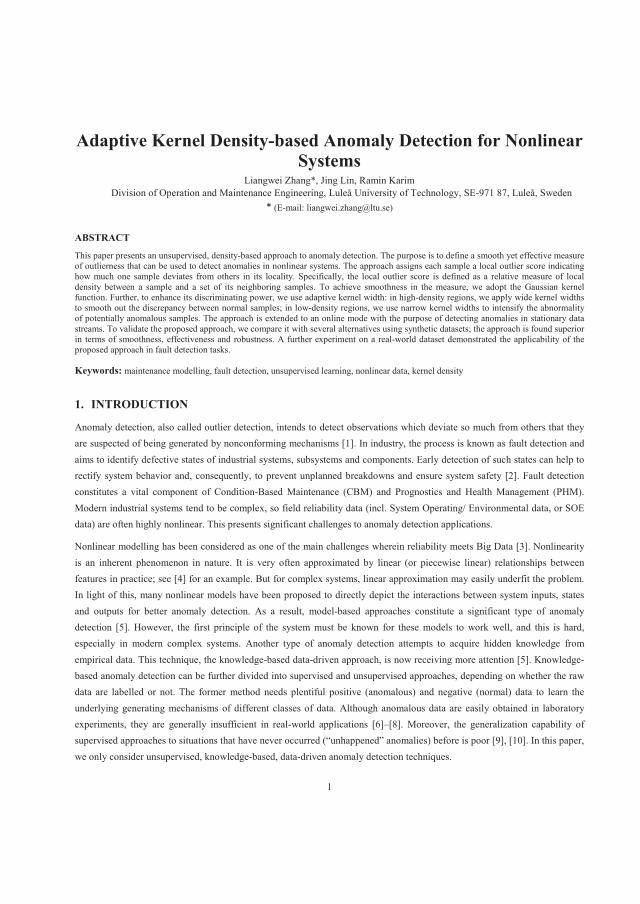
1
Adaptive Kernel Density-based Anomaly Detection for Nonlinear Systems
Liangwei Zhang*, Jing Lin, Ramin Karim Division of Operation and Maintenance Engineering, Luleå University of Technology, SE-971 87, Luleå, Sweden
* (E-mail: [email protected])
ABSTRACT
This paper presents an unsupervised, density-based approach to anomaly detection. The purpose is to define a smooth yet effective measure of outlierness that can be used to detect anomalies in nonlinear systems. The approach assigns each sample a local outlier score indicating how much one sample deviates from others in its locality. Specifically, the local outlier score is defined as a relative measure of local density between a sample and a set of its neighboring samples. To achieve smoothness in the measure, we adopt the Gaussian kernel function. Further, to enhance its discriminating power, we use adaptive kernel width: in high-density regions, we apply wide kernel widths to smooth out the discrepancy between normal samples; in low-density regions, we use narrow kernel widths to intensify the abnormality of potentially anomalous samples. The approach is extended to an online mode with the purpose of detecting anomalies in stationary data streams. To validate the proposed approach, we compare it with several alternatives using synthetic datasets; the approach is found superior in terms of smoothness, effectiveness and robustness. A further experiment on a real-world dataset demonstrated the applicability of the proposed approach in fault detection tasks.
Keywords: maintenance modelling, fault detection, unsupervised learning, nonlinear data, kernel density
1. INTRODUCTION
Anomaly detection, also called outlier detection, intends to detect observations which deviate so much from others that they are suspected of being generated by nonconforming mechanisms [1]. In industry, the process is known as fault detection and aims to identify defective states of industrial systems, subsystems and components. Early detection of such states can help to rectify system behavior and, consequently, to prevent unplanned breakdowns and ensure system safety [2]. Fault detection constitutes a vital component of Condition-Based Maintenance (CBM) and Prognostics and Health Management (PHM). Modern industrial systems tend to be complex, so field reliability data (incl. System Operating/ Environmental data, or SOE data) are often highly nonlinear. This presents significant challenges to anomaly detection applications.
Nonlinear modelling has been considered as one of the main challenges wherein reliability meets Big Data [3]. Nonlinearity is an inherent phenomenon in nature. It is very often approximated by linear (or piecewise linear) relationships between features in practice; see [4] for an example. But for complex systems, linear approximation may easily underfit the problem. In light of this, many nonlinear models have been proposed to directly depict the interactions between system inputs, states and outputs for better anomaly detection. As a result, model-based approaches constitute a significant type of anomaly detection [5]. However, the first principle of the system must be known for these models to work well, and this is hard, especially in modern complex systems. Another type of anomaly detection attempts to acquire hidden knowledge from empirical data. This technique, the knowledge-based data-driven approach, is now receiving more attention [5]. Knowledge-based anomaly detection can be further divided into supervised and unsupervised approaches, depending on whether the raw data are labelled or not. The former method needs plentiful positive (anomalous) and negative (normal) data to learn the underlying generating mechanisms of different classes of data. Although anomalous data are easily obtained in laboratory experiments, they are generally insufficient in real-world applications [6]–[8]. Moreover, the generalization capability of supervised approaches to situations that have never occurred (“unhappened” anomalies) before is poor [9], [10]. In this paper, we only consider unsupervised, knowledge-based, data-driven anomaly detection techniques.

2
In the unsupervised regime, many existing anomaly detection techniques can deal with nonlinearity to a different extent. First, statistical methods detect anomalies based on the low probability of sample generation. Parametric ones typically require extensive a priori knowledge on the application to make strong assumptions on the data distribution; an example is the Gaussian Mixture Model (GMM) [11]. Non-parametric methods, such as the Parzen window estimator, estimate the probability density of data distribution using some smooth functions and then set a threshold to single out anomalies [12], [13]. Although they make no assumptions on the data distribution, they may perform badly when different density regions exist in the data. Second, density-based approaches (in a spatial sense) are another type of nonlinear technique in anomaly detection; of these, the Local Outlier Factor (LOF) approach is the best known. LOF is free of assumptions on the data distributions and has many desired properties, such as computational simplicity [14]. However, the metric local outlier factor is discontinuous and highly dependent on its input parameter. Third, an Artificial Neural Network (ANN) can handle nonlinearity because of its nonlinear activation function and multi-layer architecture. Self-Organizing Map (SOM) is a typical unsupervised ANN; it learns to cluster groups of similar input patterns onto low-dimensional output spaces (most commonly a two-dimensional discrete lattice). Even though SOM has been used in anomaly detection applications [15], its original purpose was dimensionality reduction or clustering, not anomaly detection. Last but not least, in the machine learning field, the kernel method is a common trick to deal with nonlinearity. In the kernel method, nonlinear transformations are conducted from the original input space to a high-dimensional (possibly infinite) feature space. Traditional linear approaches applied in the feature space can then tackle nonlinear problems in the original input space. Examples in the context of anomaly detection include Support Vector Data Description (SVDD) and Kernel Principal Component Analysis (KPCA), and so on [16], [17]. The main problem with this type of learning is the lack of interpretability and the difficulty of tuning input parameters in an unsupervised fashion. An inappropriate setting of input parameters may easily lead to underfitting or overfitting.
In this paper, we propose an adaptive kernel density-based anomaly detection (Adaptive-KD for simplicity) approach with the purpose of detecting anomalies in nonlinear systems. The approach is instance-based and assigns a degree of being an anomaly to each sample, i.e., a local outlier score. Specifically, the local outlier score is a relative measure of local density between a point and a set of its reference points. Here, the reference set is simply defined as geometrically neighboring points that are presumed to resemble similar data generating mechanisms. The measure local density is defined via a smooth kernel function. The main novelty is that when computing local density, the kernel width parameter is adaptively set depending on the average distance from one candidate to its neighboring points: the larger the distance, the narrower the width, and vice versa. The method allows the contrast between potentially anomalous and normal points to be highlighted and the discrepancy between normal points to be smoothed out, something desired in anomaly detection applications. We extend the approach to an online mode to conduct anomaly detection from stationary data streams. To evaluate the proposed approach, we compare it with several alternatives using both synthetic and real-world datasets. The results demonstrate the efficacy of our approach in terms of smoothness, effectiveness, and robustness.
The rest of the paper proceeds as follows. In Section 2, we introduce two density-based anomaly detection approaches that are closely related to this research. The discussion of the strengths and weaknesses of these two approaches leads to our explanation of the original motivation for this study. We present the Adaptive-KD approach in Section 3; in this section, we focus on the computation of local density using adaptive kernel width. The approach is then consolidated to an integrated algorithm and extended to an online mode to detect anomalies in a stationary data stream. In Section 4, we compare the smoothness, effectiveness, and robustness of our approach with several alternatives, including LOF, SVDD and KPCA, using
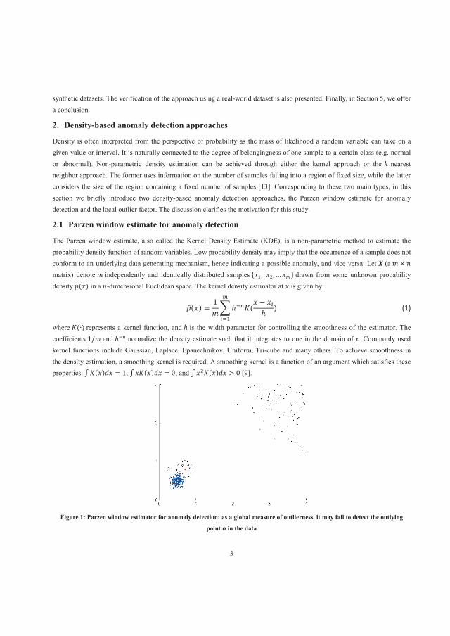
3
synthetic datasets. The verification of the approach using a real-world dataset is also presented. Finally, in Section 5, we offer a conclusion.
2. Density-based anomaly detection approaches
Density is often interpreted from the perspective of probability as the mass of likelihood a random variable can take on a given value or interval. It is naturally connected to the degree of belongingness of one sample to a certain class (e.g. normal or abnormal). Non-parametric density estimation can be achieved through either the kernel approach or the nearest neighbor approach. The former uses information on the number of samples falling into a region of fixed size, while the latter considers the size of the region containing a fixed number of samples [13]. Corresponding to these two main types, in this section we briefly introduce two density-based anomaly detection approaches, the Parzen window estimate for anomaly detection and the local outlier factor. The discussion clarifies the motivation for this study.
2.1 Parzen window estimate for anomaly detection
The Parzen window estimate, also called the Kernel Density Estimate (KDE), is a non-parametric method to estimate the probability density function of random variables. Low probability density may imply that the occurrence of a sample does not conform to an underlying data generating mechanism, hence indicating a possible anomaly, and vice versa. Let (a × matrix) denote independently and identically distributed samples { , , … } drawn from some unknown probability density ( ) in a -dimensional Euclidean space. The kernel density estimator at is given by: ( ) = 1 ( ) (1)
where ( ) represents a kernel function, and is the width parameter for controlling the smoothness of the estimator. The coefficients 1/ and normalize the density estimate such that it integrates to one in the domain of . Commonly used kernel functions include Gaussian, Laplace, Epanechnikov, Uniform, Tri-cube and many others. To achieve smoothness in the density estimation, a smoothing kernel is required. A smoothing kernel is a function of an argument which satisfies these properties: ( ) = 1, ( ) = 0, and ( ) > 0 [9].
Figure 1: Parzen window estimator for anomaly detection; as a global measure of outlierness, it may fail to detect the outlying
point in the data
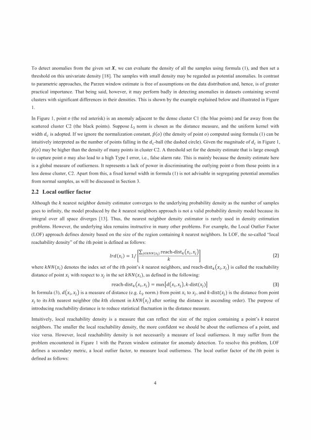
4
To detect anomalies from the given set , we can evaluate the density of all the samples using formula (1), and then set a threshold on this univariate density [18]. The samples with small density may be regarded as potential anomalies. In contrast to parametric approaches, the Parzen window estimate is free of assumptions on the data distribution and, hence, is of greater practical importance. That being said, however, it may perform badly in detecting anomalies in datasets containing several clusters with significant differences in their densities. This is shown by the example explained below and illustrated in Figure 1.
In Figure 1, point (the red asterisk) is an anomaly adjacent to the dense cluster C1 (the blue points) and far away from the scattered cluster C2 (the black points). Suppose norm is chosen as the distance measure, and the uniform kernel with width is adopted. If we ignore the normalization constant, ( ) (the density of point ) computed using formula (1) can be intuitively interpreted as the number of points falling in the -ball (the dashed circle). Given the magnitude of in Figure 1, ( ) may be higher than the density of many points in cluster C2. A threshold set for the density estimate that is large enough to capture point may also lead to a high Type I error, i.e., false alarm rate. This is mainly because the density estimate here is a global measure of outlierness. It represents a lack of power in discriminating the outlying point from those points in a less dense cluster, C2. Apart from this, a fixed kernel width in formula (1) is not advisable in segregating potential anomalies from normal samples, as will be discussed in Section 3.
2.2 Local outlier factor
Although the nearest neighbor density estimator converges to the underlying probability density as the number of samples goes to infinity, the model produced by the nearest neighbors approach is not a valid probability density model because its integral over all space diverges [13]. Thus, the nearest neighbor density estimator is rarely used in density estimation problems. However, the underlying idea remains instructive in many other problems. For example, the Local Outlier Factor (LOF) approach defines density based on the size of the region containing nearest neighbors. In LOF, the so-called “local reachability density” of the th point is defined as follows:
( ) = 1/ reach-dist ,( ) (2)
where ( ) denotes the index set of the th point’s nearest neighbors, and reach-dist , is called the reachability distance of point with respect to in the set ( ), as defined in the following:
reach-dist , = max , , -dist( ) (3) In formula (3), , is a measure of distance (e.g. norm.) from point to , and -dist( ) is the distance from point
to its th nearest neighbor (the th element in after sorting the distance in ascending order). The purpose of introducing reachability distance is to reduce statistical fluctuation in the distance measure.
Intuitively, local reachability density is a measure that can reflect the size of the region containing a point’s nearest neighbors. The smaller the local reachability density, the more confident we should be about the outlierness of a point, and vice versa. However, local reachability density is not necessarily a measure of local outlierness. It may suffer from the problem encountered in Figure 1 with the Parzen window estimator for anomaly detection. To resolve this problem, LOF defines a secondary metric, a local outlier factor, to measure local outlierness. The local outlier factor of the th point is defined as follows:

5
( ) = 1 ( )( )( ) (4)
This is a relative measure computing the quotient between the average local reachability densities of a point’s nearest neighbors and the point’s own local reachability density. Typically, points with a local outlier factor around (or less than) one should be considered normal, as their densities are roughly the same as (or larger than) the average density of their neighbouring points. A point with a local outlier factor remarkably larger than one is more likely to be an anomaly.
The key to defining a local outlierness measure (e.g., a local outlier score) is to compare the primary metric (e.g., local reachability density) of a point with those of its reference points (e.g., nearest neighbors). Based on the LOF approach and many of its variants, a recent study has pointed out that the importance of defining the outlierness measure in a local sense is that a local outlierness measure is relatively more invariant to the fluctuations in the density estimate and, hence, is more comparable over a dataset with varying densities [19].
Despite its extensive applications in the real world, the LOF approach has two drawbacks: First, the primary metric (local reachability density) is not smooth, and this may cause discontinuities in the measure of the local outlier factor, as will be shown in Section 4. Second, its accuracy is very sensitive to the input parameter, namely, the number of nearest neighbors. A bad selection of this parameter can easily conceal the structure in the data and lead to a failure to detect potential anomalies; see Figure 6 (1.d) for an example.
With the aim of fostering the strengths of and circumventing the weaknesses in the above two approaches, this study combines them to get a smooth local outlierness measure that can detect anomalies from nonlinear data. The LOF approach provides a basic scheme for defining local outlierness, while the idea of using kernel functions in the Parzen window estimate approach is helpful in deriving a smooth density estimate. To enhance the discriminating power of the local outlierness measure, we explore the use of flexible kernel widths, as has been done in some “adaptive” kernel density estimation approaches.
3. Adaptive kernel density-based anomaly detection approach
Anomaly detection aims to identify observations which deviate so much from others that they are suspected of being generated by nonconforming mechanisms. A desirable anomaly detection approach should not only produce a binary output (abnormal or normal) but also assign a degree of being an anomaly to each observation. Based upon the two approaches introduced above, this section suggests using an adaptive kernel density-based approach to measure this degree of deviation. We start with the general idea of the approach; we then introduce the computation into local density and local outlier scores. We consolidate the parts in an integrated algorithm and extend it to an online mode. Finally, we discuss the time complexity.
3.1 General idea of the approach
The main purpose of the Adaptive-KD approach is to compute the degree of deviation of data points in a local sense. The significance of measuring the outlierness of a point locally has been highlighted in Section 2. To maintain a uniform notation, we follow the definition in Section 2 and let be a given dataset containing data points in R . The Adaptive-KD approach attempts to define a function mapping from to a real valued vector in R ; i.e., : , where ( ) represents the -th point’s local outlier score.
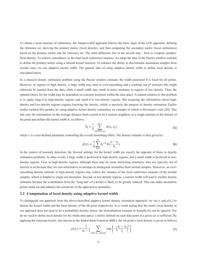
6
To obtain a local measure of outlierness, the Adaptive-KD approach follows the basic steps of the LOF approach: defining the reference set, deriving the primary metric (local density), and then computing the secondary metric (local outlierness) based on the primary metric and the reference set. The main difference lies in the second step – how to compute samples’ local density. To achieve smoothness in the final local outlierness measure, we adopt the idea of the Parzen window estimate to define the primary metric using a smooth kernel function. To enhance the ability to discriminate anomalous samples from normal ones, we use adaptive kernel width. The general idea of using adaptive kernel width to define local density is elucidated below.
In a classical density estimation problem using the Parzen window estimate, the width parameter is fixed for all points. However, in regions of high density, a large width may lead to over-smoothing and a washing out of structure that might otherwise be learned from the data, while a small width may result in noisy estimates in regions of low density. Thus, the optimal choice for the width may be dependent on concrete locations within the data space. A natural solution to this problem is to apply large in high-density regions and small in low-density regions. But acquiring the information about high-density and low-density regions requires knowing the density, which is precisely the purpose of density estimation. Earlier studies tackled this paradox by using adaptive kernel density estimation, an example of which is Silverman’s rule [20]. This rule uses the information on the average distance from a point to its nearest neighbors as a rough estimate to the density of the point and defines the kernel width as follows:
= ( , )( ) (5)
where is a user-defined parameter controlling the overall smoothing effect. The density estimate is then given by:
( ) = 1 ( ) (6)
In the context of anomaly detection, the favored settings for the kernel width are exactly the opposite of those in density estimation problems. In other words, a large width is preferred in high-density regions, and a small width is preferred in low-density regions. First, in high-density regions, although there may be some interesting structures, they are typically not of interest to us because they are non-informative in attempts to distinguish anomalies from normal samples. Moreover, an over-smoothing density estimate in high-density regions may reduce the variance of the local outlierness measure of the normal samples, which is helpful to single out anomalies. Second, in low-density regions, a narrow width will lead to smaller density estimates because the contribution from the “long tail” of a kernel is likely to be greatly reduced. This can make anomalous points stand out and enhance the sensitivity of the approach to anomalies.
3.2 Computation of local density using adaptive kernel width
To distinguish our approach from the above-described adaptive kernel density estimation approach, we use and ( ) to denote the kernel width and the local density of the th point respectively. It is worth noting that the metric local density in our approach does not need to be a probability density; hence, the normalization constant in formula (6) can be ignored. Nor do we need to define local density for the whole data space; a metric defined on each data point in a given set is sufficient. By applying the Gaussian kernel, also known as the Radial Basis Function (RBF), the th point’s local density is given as follows:
( ) = 1 1 exp{ , ,…, }\{ } (7)

7
The right-hand side of formula (7) excludes the contribution from the th point itself (i.e., exp{ ( ) } = 1) in the summation. The purpose is to highlight the relative difference in density between different points (e.g., the quantity 0.1 0.3 is much less than the quantity 1.1/1.3). In addition, the subscript of the kernel width in formula (7) is different from the one in formula (6). It is only associated with the point of our concern, leading to a simple explanation of one point’s local density as the following: the average contribution from the remaining points in the Gaussian kernel with a locality dependent width. A more intuitive interpretation is illustrated by a one-dimensional example containing five points { , , , , } in Figure 2 (a). The point ’s local density is the average height of the blue, solid, vertical lines underneath the Gaussian kernel evaluation. From Figure 2 (a), it is also evident that local density reflects the extent to which one point is supported by others. The more neighboring points close to the point of concern, the larger its local density, and vice versa.
As argued above, the width should be locality dependent. A large is preferred in high-density regions and a small one in low-density regions. This is intuitively demonstrated in Figure 2 (b) where the kernel evaluations of three different points are plotted. The leftmost bell curve (in red) corresponding to the outlying point has the narrowest shape. The middle bell curve (in black) associated with has the widest shape because the point is near the center. The rightmost bell curve (in green) is associated with and has an intermediate width. As expected, this locality dependent width will lead to two results: points that are far away from others will be more isolated, and the discrepancy between normal points will be blurred.
Figure 2: Illustration of (a) definition of local density, and (b) locality dependent width
Now, we discuss how to adaptively set the width parameter in formula (7). Given the role of kernel width, we restrict it to be strictly positive. For the th point, we let ( ) denote the average distance to its nearest neighbors; i.e., ( ) =(1 ) ( , ){ } . Further, we let -max and -min , respectively, be the largest and the smallest quantity in the set { ( )| = 1,2, … , }. Similar to Silverman’s rule, we can first use ( ) as a rough estimate of points’ density and then construct a negative correlation between the width and ( ). Given these requirements, we define the th point’s width as follows: = [ -max + -min + ( )] (8)
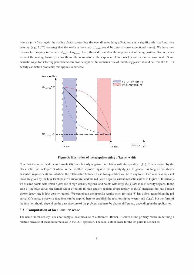
8
where ( > 0) is again the scaling factor controlling the overall smoothing effect, and is a significantly small positive quantity (e.g., 10 ) ensuring that the width is non-zero ( -min could be zero in some exceptional cases). We have two reasons for bringing in the term -max + -min. First, the width satisfies the requirement of being positive. Second, even without the scaling factor , the width and the numerator in the exponent of formula (7) will be on the same scale. Some heuristic ways for selecting parameter can now be applied. Silverman’s rule of thumb suggests should be from 0.5 to 1 in density estimation problems; this applies in our case.
Figure 3: Illustration of the adaptive setting of kernel width
Note that the kernel width in formula (8) has a linearly negative correlation with the quantity ( ). This is shown by the black solid line in Figure 3 where kernel width is plotted against the quantity ( ). In general, as long as the above-described requirements are satisfied, the relationship between these two quantities can be of any form. Two other examples of these are given by the blue (with positive curvature) and the red (with negative curvature) solid curves in Figure 3. Informally, we assume points with small ( ) are in high-density regions, and points with large ( ) are in low-density regions. In the case of the blue curve, the kernel width of points in high-density regions drops rapidly as ( ) increases but has a much slower decay rate in low-density regions. We can obtain the opposite results when formula (8) has a form resembling the red curve. Of course, piecewise functions can be applied here to establish the relationship between and ( ), but the form of the function should depend on the data structure of the problem and may be chosen differently depending on the application.
3.3 Computation of local outlier score
The name “local density” does not imply a local measure of outlierness. Rather, it serves as the primary metric in defining a relative measure of local outlierness, as in the LOF approach. The local outlier score for the th point is defined as:
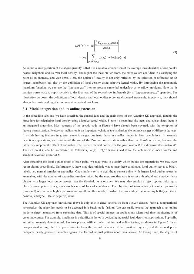
9
( ) = log 1 ( )( )( ) = log ( )( ) log[ ( )]
(9)
An intuitive interpretation of the above quantity is that it is a relative comparison of the average local densities of one point’s nearest neighbors and its own local density. The higher the local outlier score, the more we are confident in classifying the point as an anomaly, and vice versa. Here, the notion of locality is not only reflected by the selection of reference set ( nearest neighbors), but also by the definition of local density using adaptive kernel width. By introducing the monotonic logarithm function, we can use the “log-sum-exp” trick to prevent numerical underflow or overflow problems. Note that it requires some work to apply the trick to the first term of the second row in formula (9), a “log-sum-sum-exp” operation. For illustrative purposes, the definitions of local density and local outlier score are discussed separately; in practice, they should always be considered together to prevent numerical problems.
3.4 Model integration and its online extension
In the preceding sections, we have described the general idea and the main steps of the Adaptive-KD approach, notably the procedure for calculating local density using adaptive kernel width. Figure 4 streamlines the steps and consolidates them in an integrated algorithm. Most contents of the pseudo code in Figure 4 have already been covered, with the exception of feature normalization. Feature normalization is an important technique to standardize the numeric ranges of different features. It avoids having features in greater numeric ranges dominate those in smaller ranges in later calculations. In anomaly detection applications, we recommend the use of the Z-score normalization rather than the Min-Max scaling because the latter may suppress the effect of anomalies. The Z-score method normalizes the given matrix to a dimensionless matrix . The -th point can be normalized as follows: = ( ) , where and are the column-wise mean vector and standard deviation vector of .
After obtaining the local outlier score of each point, we may want to classify which points are anomalous; we may even report alarms accordingly. Unfortunately, there is no deterministic way to map these continuous local outlier scores to binary labels, i.e., normal samples or anomalies. One simple way is to treat the top-most points with largest local outlier scores as anomalies, with the number of anomalies pre-determined by the user. Another way is to set a threshold and consider those objects with larger local outlier scores than the threshold as anomalies. We may also employ a reject option, refusing to classify some points to a given class because of lack of confidence. The objective of introducing yet another parameter (threshold) is to achieve higher precision and recall, in other words, to reduce the probability of committing both type I (false positive) and type II (false negative) error.
The Adaptive-KD approach introduced above is only able to detect anomalies from a given dataset. From a computational perspective, the algorithm needs to be executed in a batch-mode fashion. We can easily extend the approach to an online mode to detect anomalies from streaming data. This is of special interest in applications where real-time monitoring is of great importance. For example, timeliness is a significant factor in designing industrial fault detection applications. Typically, an online anomaly detection task has two phases: offline model training and online testing, as shown in Figure 5. In an unsupervised setting, the first phase tries to learn the normal behavior of the monitored system, and the second phase compares newly generated samples against the learned normal pattern upon their arrival. At testing time, the degree of

10
deviation of a sample from the normal pattern is used as evidence to discriminate anomalies from normal samples. This type of scheme is also known as one-class anomaly detection in machine learning, as it requires the training set to be restricted to negative samples (i.e., normal samples). Assuming the training set and testing set are already preprocessed, we explain the online extension of the Adaptive-KD approach in the following.
Algorithm 1 -- ( , , )
BEGIN Initialize ; Conduct feature normalization on , and save it to matrix ; Compute pairwise distance ( , ) for all , {1,2, … , }, ; FOREACH Derive the reference set: nearest neighbors ( ) by sorting the above distances; Calculate the average distance to its nearest neighbors ( ); END Obtain -min and -max from all the quantities ( ) where {1,2, … , }; FOREACH
Compute the kernel width of the th point using formula (8); Compute the local density of the th point ( ) using formula (7);
END FOREACH
Compute the local outlier score ( ) using formula (9); END RETURN ;
END
Figure 4: Adaptive kernel density based anomaly detection (Adaptive-KD) algorithm
The offline model training phase, as shown in Figure 5, basically follows the procedure of the Adaptive-KD algorithm in Figure 4. Since this phase intends to learn the pattern of system normal behavior, it is worthwhile to meticulously select anomalous-free samples to construct the training set. The existence of anomalies may reduce the local outlier score of samples at testing time and could possibly lead to missed detections. To solve this, we add a data refinement procedure to exclude those samples with remarkably high local outlier scores from the training set and then retrain the model. Although the condition as to when data refinement is needed is somewhat subjective, it gives us a way to select representative training sets. This is often not possible in one-class anomaly detection approaches, such as the SVDD approach.
The normal pattern learned in the first phase is yielded as model parameters which are used in the second phase. Since the Adaptive-KD approach is an instance-based approach, the model parameters consist of all samples in the training set (possibly refined in the first phase) and their local densities. Other intermediate parameters that can be reused in the testing phase should also be included. For example, parameters and are required to rescale online samples, and -min and -max are necessary for computing kernel width of samples at testing time. Notably, our model’s parameters are fixed once trained. The fundamental assumption of this online extension is that the normal behavior of the system does not evolve as time goes on (no concept drift in the data stream). In other words, the monitored system is presumed to be stationary, or the change in the system normal behavior is negligible in the monitoring period. We can also retrain the model regularly to absorb normal changes in the system.
The online testing phase takes in real-time samples and computes their local outlier scores sequentially. A single testing sample goes through a routine similar to that of the first phase. Model parameters learned in the first phase provide necessary
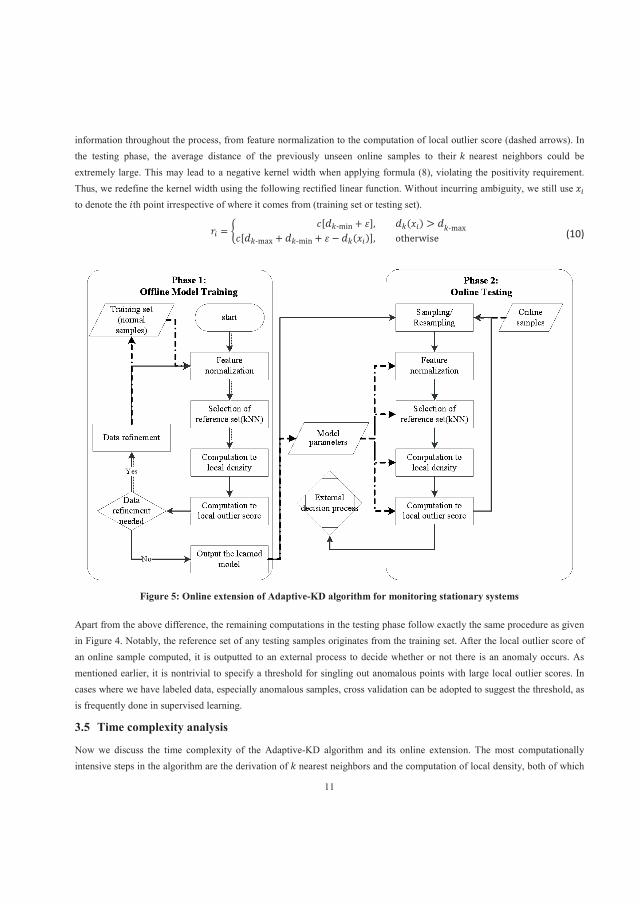
11
information throughout the process, from feature normalization to the computation of local outlier score (dashed arrows). In the testing phase, the average distance of the previously unseen online samples to their nearest neighbors could be extremely large. This may lead to a negative kernel width when applying formula (8), violating the positivity requirement. Thus, we redefine the kernel width using the following rectified linear function. Without incurring ambiguity, we still use to denote the th point irrespective of where it comes from (training set or testing set). = [ -min + ], ( ) > -max[ -max + -min + ( )], otherwise (10)
Figure 5: Online extension of Adaptive-KD algorithm for monitoring stationary systems
Apart from the above difference, the remaining computations in the testing phase follow exactly the same procedure as given in Figure 4. Notably, the reference set of any testing samples originates from the training set. After the local outlier score of an online sample computed, it is outputted to an external process to decide whether or not there is an anomaly occurs. As mentioned earlier, it is nontrivial to specify a threshold for singling out anomalous points with large local outlier scores. In cases where we have labeled data, especially anomalous samples, cross validation can be adopted to suggest the threshold, as is frequently done in supervised learning.
3.5 Time complexity analysis
Now we discuss the time complexity of the Adaptive-KD algorithm and its online extension. The most computationally intensive steps in the algorithm are the derivation of nearest neighbors and the computation of local density, both of which

12
take the time complexity of ( max ( , )). Thus, the overall time complexity for the primitive Adaptive-KD algorithm and the offline model training phase (assuming there are data points in the training set) of its extension are (max ( , )). It is possible to reduce the computational cost by applying the following considerations to the above two steps.
Locality dependent kernel width is better than choosing a uniformly constant kernel width. However, this increases the computational complexity of performing local density evaluation, as it requires finding nearest neighbors before figuring out the kernel width of points. A typical way to reduce the time complexity of finding nearest neighbors is to employ an indexing structure, such as - tree or R tree. The time complexity can be reduced to ( log ( ) max ( , )) at the expense of additional memory space. Another improvement, random projection, can alleviate the high computational cost of finding nearest neighbors when the dimensionality is high. This is supported by the Johnson-Lindenstrauss theorem claiming that a set of points in a high-dimensional Euclidean space can be embedded into a (log ( / )) dimensional Euclidean space such that any pairwise distance changes only by a factor of (1 ± ) [21].
The complication of local density computation lies in the Gaussian kernel evaluation, mainly because the Gaussian kernel has an unbounded support. In other words, the Gaussian kernel function needs to be evaluated for each point with respect to all remaining points. While the shape of the kernel function may important in theoretical research, from a practical perspective, it matters far less than the width parameter. Thus, other kernel functions with compact support, such as the Epanechnikov or the Tri-cube kernel, can be adopted. However, they require introducing additional parameters to determine the size of their support. Typically, only those points with a distance less than a given threshold to the point of interest will be evaluated using the chosen kernel function.
The online testing phase of the algorithm’s extension continuously processes new samples upon their arrival. The time complexity of this phase is much more important in the sense that it decides whether the algorithm can give real-time or near real-time responses to a fast-flowing data stream. It is necessary to maintain those model parameters yielded from the training phase to avoid repetitive computations at testing time. This is where the concept of trading space for time applies. As in the offline model training phase, the most computationally demanding steps in the online testing phase are the derivation of nearest neighbors and the computation of local density, both of which have a time complexity of ( max ( , )). With the same considerations as discussed before, the computational cost can be vastly reduced.
4. Numerical illustration
This section evaluates the proposed approach using synthetic datasets and a real-world dataset. Concretely, we contrast the online extension of our approach with the LOF online extension, SVDD and KPCA using synthetic datasets. Then we compare the Adaptive-KD algorithm with LOF and Parzen window estimate approach using a dataset from the railway industry. Before diving into the numerical examples, we briefly introduce some uncovered approaches which are chosen here for comparison.
Building on the idea introduced in Subsection 3.4, the LOF approach can be extended to an online mode, the application of which is explained by [22]. The SVDD approach applies the “kernel trick” to implicitly conduct nonlinear mapping from the original input space to a high-dimensional feature space. It tries to find a minimum volume hyper-sphere that can enclose normal samples in the feature space [23]. For any testing sample, the outlierness measure is the difference between the distance from the testing sample to the hyper-sphere center and the radius of the hyper-sphere. The larger the measure, the more likely the sample is to be anomalous. The hyper-sphere can be obtained by minimizing an objective function containing

13
two terms: the first measures the volume of the hyper-sphere; the second penalizes larger distances from samples to the hyper-sphere center. An input parameter is needed to address the trade-off between the two. In the following experiments, we use the Gaussian kernel with an input parameter as the kernel width.
The KPCA approach is based on the spectral theory, which assumes normal samples and anomalies appear as significant discrepancies in a lower-dimensional subspace embedding. Similar to the SVDD approach, KPCA applies the “kernel trick” to extend Principle Component Analysis (PCA) to nonlinear cases. It learns the normal pattern from a training set by retaining most of the variance in the principal components. Then, the reconstruction error of the testing samples is used to depict their degree of outlierness [24]. The higher the reconstruction error, the more a testing sample disagrees with the learned pattern and the more likely it is to be an anomaly. In the following experiments, we use the Gaussian kernel with width parameter . Further, we let denote the proportion of variance retained in subspace.
4.1 Smoothness test on the “aggregation” dataset
In previous sections, we claimed our approach defines a smooth local outlierness measure. To justify this claim, we apply the online extension of the approach to the “aggregation” dataset and compare it with other alternatives. As shown in Figure 6 (1.a), the “aggregation” dataset contains 788 samples forming seven different clusters. The purpose is not to detect anomalies in this dataset. Instead, these samples constitute the training set, and they are considered normal. The testing set is obtained by discretizing the horizontal axis (from 0 to 40) and the vertical axis (from 0 to 30) using a step size 0.2. This leads to a two-dimensional grid with 30351 (151 201) intersecting points, i.e., the testing set. Training sets consisting of multiple clusters are common in reality. Each cluster represents a normal behavior of the monitored system running in a particular operational mode.
For all the anomaly detection approaches introduced so far, each testing sample can be assigned a degree of outlierness. For comparative purposes, all the outlierness measures are standardized to a range from 0 to 1. The larger the measure is, the more likely a testing sample is to be anomalous. In Figure 6, from subplot (1.b) to (1.h), each testing sample is marked using a colored point in the coordinate system. As indicated by the color bar, the degree of outlierness increases as the color evolves from dark blue to dark red. Each subplot from (1.b) to (1.h) corresponds to a particular approach under a specific parameter setting. The influence of parameters and to our approach will be explained later. Here, we simply present the result of our approach when = 1 and = 40. To illustrate how the LOF approach is affected by parameter , we try two different settings: = 20 and = 40. As suggested in the original paper on the SVDD approach, the trade-off parameter should take value 1 when the training set is noiseless. Thus, we only vary the width parameter in the experiment. We fix parameter at 0.9 and vary the kernel width in the KPCA approach. The corresponding contour curves of the degree of outlierness are given in subplots (2.b) to (2.h).
An ideal approach should be able to detect the nonlinear shape of the clusters. Samples are also expected to have a low degree of outlierness when they fall inside the clusters, and a large degree when they are away from the clusters. Moreover, the transition in the outlierness measure from cluster cores to cluster halos should be smooth. As subplots (1.b) and (2.b) suggest, our approach can correctly detect the shape of the clusters and give a very smooth local outlierness measure. In addition, the results are fairly robust to the change of parameter in this example. Another example of the contour plot when parameter = 20 is presented in subplot (2.a). Notice that in the cluster cores, the local outlierness scores are almost identical. This is caused by the smoothing effect of large kernel width in high-density regions.
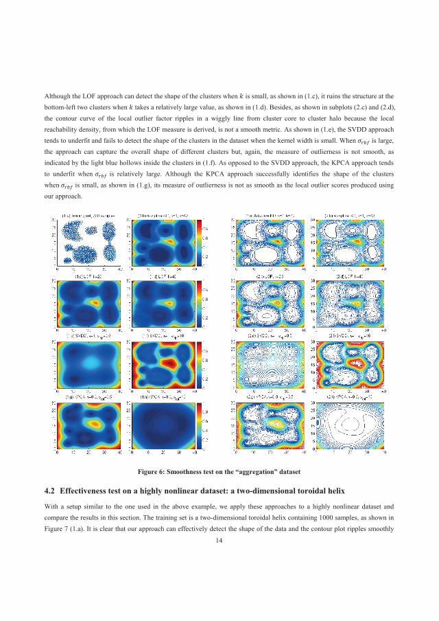
14
Although the LOF approach can detect the shape of the clusters when is small, as shown in (1.c), it ruins the structure at the bottom-left two clusters when takes a relatively large value, as shown in (1.d). Besides, as shown in subplots (2.c) and (2.d), the contour curve of the local outlier factor ripples in a wiggly line from cluster core to cluster halo because the local reachability density, from which the LOF measure is derived, is not a smooth metric. As shown in (1.e), the SVDD approach tends to underfit and fails to detect the shape of the clusters in the dataset when the kernel width is small. When is large, the approach can capture the overall shape of different clusters but, again, the measure of outlierness is not smooth, as indicated by the light blue hollows inside the clusters in (1.f). As opposed to the SVDD approach, the KPCA approach tends to underfit when is relatively large. Although the KPCA approach successfully identifies the shape of the clusters when is small, as shown in (1.g), its measure of outlierness is not as smooth as the local outlier scores produced using our approach.
Figure 6: Smoothness test on the “aggregation” dataset
4.2 Effectiveness test on a highly nonlinear dataset: a two-dimensional toroidal helix
With a setup similar to the one used in the above example, we apply these approaches to a highly nonlinear dataset and compare the results in this section. The training set is a two-dimensional toroidal helix containing 1000 samples, as shown in Figure 7 (1.a). It is clear that our approach can effectively detect the shape of the data and the contour plot ripples smoothly

15
towards both outside and inside hollows, as shown in Figure 7 (1.b) and (2.b). Again, the LOF approach can somewhat recognize the shape of the data. But the contour plot is rather uneven, and the discontinuities in the measure of local outlierness is significant, especially when takes a large value. The SVDD approach detects the shape when the kernel width is large, while the KPCA approach works when the width parameter is small. It seems SVDD performs better than KPCA in the interior of the toroidal helix. However, the outlierness measure of all three alternatives is not as smooth as we expected.
As we vary parameter while fixing in our approach, the results could appear to be over-smoothing or under-smoothing. This is mainly because the kernel width defined in formula (8) is also affected by parameter . In general, a small will lead to a small ( ) and , thereby decreasing the overall smoothing effect. The phenomenon can be compensated for by choosing a larger . In Figure 7 (2.a), we present another comparable result; in this example, = 0.8 and = 10. The effect of over-smoothing and under-smoothing is elaborated in detail in the next subsection.
Figure 7: Effectiveness test on a two-dimensional toroidal helix dataset
In the above two examples, the purpose is to compare our approach with the selected alternatives. Even though a global measure of outlierness derived from a well-tuned kernel density estimator can achieve comparable smoothness in these examples, it may fail in a dataset where clusters have significant differences in their densities, as we argued in Subsection 2.1.

16
4.3 Robustness test on the “flame” dataset
In the following, we use the “flame” dataset to show how the existence of anomalies in the training set affects these approaches. We also discuss the robustness of our approach to the perturbation of input parameters. The “flame” dataset is shown in Figure 8 (1.a); the top-left-most two points are considered anomalies. The remaining sub-graphs in Figure 8 agree with our assessment of the smoothness and effectiveness of these approaches in the previous two examples. They also demonstrate that all approaches are affected by the two anomalies, albeit to a different extent. As described earlier, the Adaptive-KD approach naturally has the ability to assign a local outlier score to any sample in the training set. Thus, the data refinement step in the offline training stage should be able to capture and discard these two anomalies and then retrain a model on the refined set. The LOF approach can recognize the two anomalies with the same routine. However, it is non-trivial for the SVDD and KPCA approach to mitigate the effect exerted by anomalies in the training set.
Figure 8: Robustness test on the existence of anomalies in the training set
The impacts of perturbing input parameters on our approach are presented in Figure 9. First, we vary parameter while fixing ; the results are shown in (1.a) and (1.b), the corresponding contour plots of which are given in (2.a) and (2.b). As expected, parameter directly controls the overall smoothing effect. A small may cause the fine details in the data to be
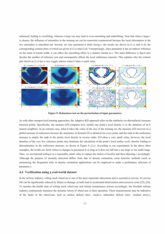
17
enhanced, leading to overfitting, whereas a large one may lead to over-smoothing and underfitting. Note that when a large is chosen, the influence of anomalies in the training set can be somewhat counteracted because the local information at the two anomalies is smoothed out. Second, we vary parameter while fixing ; the results are shown in (1.c) and (1.d), the corresponding contour plots of which are given in (2.c) and (2.d). Unsurprisingly, since parameter has an indirect influence on the scale of kernel width, it can affect the smoothing effect in a manner similar to . The main difference is that also decides the number of reference sets and consequently affects the local outlierness measure. This explains why the contour plot shown in (2.c) has a very wiggly interior when takes a small value.
Figure 9: Robustness test on the perturbation of input parameters
As with other unsupervised learning approaches, the Adaptive-KD approach relies on the similarity (or dissimilarity) measure between points. Specifically, the measure computes how similar one point’s local density is to the densities of its nearest neighbors. In an extreme case, when takes the value of the size of the training set, the measure recovers to a global measure of outlierness because the nominator in formula (9) is identical for every point, and the rank in the outlierness measure is simply the rank in the metric local density in reverse order. If takes a very small value, however, the local densities of the very few reference points may dominate the calculation of the point’s local outlier score, thereby leading to discontinuities in the outlierness measure, as shown in Figure 9 (2.c). According to our experiments in the above three examples, the results are fairly robust to changes in parameter as long as it does not fall into a too large or too small range. Thus, we recommend setting to a reasonably small value to capture the notion of locality and then adjusting accordingly. Although the purpose of anomaly detection differs from that of density estimation, some heuristic methods (such as minimizing the frequentist risk) in density estimation applications can be employed to make a preliminary selection of parameter .
4.4 Verification using a real-world dataset
In the railway industry, rolling stock wheel-set is one of the most important subsystems and is essential to service. Its service life can be significantly reduced by failure or damage, as both lead to accelerated deterioration and excessive costs [25], [26]. To monitor the health state of rolling stock wheel-sets and initiate maintenance actions accordingly, the Swedish railway industry continuously measures the dynamic forces of wheel-sets in their operation. These measurements may be indicative of the faults in the wheel-sets, such as surface defects (incl., cracks.), subsurface defects (incl., residual stress.),
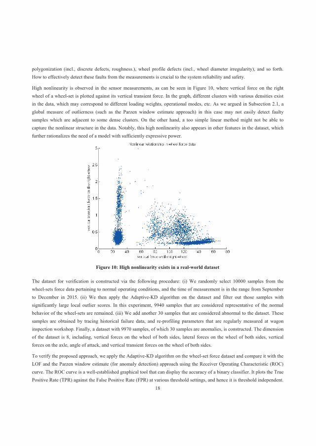
18
polygonization (incl., discrete defects, roughness.), wheel profile defects (incl., wheel diameter irregularity), and so forth. How to effectively detect these faults from the measurements is crucial to the system reliability and safety.
High nonlinearity is observed in the sensor measurements, as can be seen in Figure 10, where vertical force on the right wheel of a wheel-set is plotted against its vertical transient force. In the graph, different clusters with various densities exist in the data, which may correspond to different loading weights, operational modes, etc. As we argued in Subsection 2.1, a global measure of outlierness (such as the Parzen window estimate approach) in this case may not easily detect faulty samples which are adjacent to some dense clusters. On the other hand, a too simple linear method might not be able to capture the nonlinear structure in the data. Notably, this high nonlinearity also appears in other features in the dataset, which further rationalizes the need of a model with sufficiently expressive power.
Figure 10: High nonlinearity exists in a real-world dataset
The dataset for verification is constructed via the following procedure: (i) We randomly select 10000 samples from the wheel-sets force data pertaining to normal operating conditions, and the time of measurement is in the range from September to December in 2015. (ii) We then apply the Adaptive-KD algorithm on the dataset and filter out those samples with significantly large local outlier scores. In this experiment, 9940 samples that are considered representative of the normal behavior of the wheel-sets are remained. (iii) We add another 30 samples that are considered abnormal to the dataset. These samples are obtained by tracing historical failure data, and re-profiling parameters that are regularly measured at wagon inspection workshop. Finally, a dataset with 9970 samples, of which 30 samples are anomalies, is constructed. The dimension of the dataset is 8, including, vertical forces on the wheel of both sides, lateral forces on the wheel of both sides, vertical forces on the axle, angle of attack, and vertical transient forces on the wheel of both sides.
To verify the proposed approach, we apply the Adaptive-KD algorithm on the wheel-set force dataset and compare it with the LOF and the Parzen window estimate (for anomaly detection) approach using the Receiver Operating Characteristic (ROC) curve. The ROC curve is a well-established graphical tool that can display the accuracy of a binary classifier. It plots the True Positive Rate (TPR) against the False Positive Rate (FPR) at various threshold settings, and hence it is threshold independent.

19
The larger the area under the curve (AUC), the better accuracy a classifier can achieve. In this experiment, the parameter for both the LOF approach and our approach is set at 40, the parameter in our approach is set at 0.5, and the kernel width (the Gaussian kernel is used) for the Parzen window estimate approach is set such that points’ average number of neighbors is 2% of the sample size in the dataset. As shown in Figure 11, the Adaptive-KD approach outperforms the other two in terms of the accuracy. The AUC values of these approaches are 0.9974, 0.9828, and 0.9762, respectively. Though, seemingly, the three AUC values differ slightly, they can make a huge difference in reducing potential production losses and maintenance costs in practice.
Figure 11: ROC curve comparison to different approaches on the wheel force data
After identifying a faulty sample using our approach, one may want to further investigate the reason of declaring the abnormality of the point. This can be informative to the ensuing procedure of fault diagnosis, which intends to probe into the type, source and severity of the underlying faults. In our approach, we can trace back to all the calculations to the point’s nearest neighbors, kernel width, local density, and its local outlier score. Then, a preliminary explanation for the abnormal behavior of the recognized anomalous sample may be given. Notably, it is nontrivial to analyze the results of approaches which implicitly conduct nonlinear transformations, such as the SVDD approach. This shows another merit of our approach – interpretability – over some of the kernel methods.
5. Conclusion
This paper presents an unsupervised, density-based approach to anomaly detection from nonlinear systems. Like many other unsupervised learning approaches, it uses the similarity measure between different points and assigns each point a degree of being an anomaly, namely, a local outlier score ( ). is defined here as a relative measure of local density between a point and a set of its neighboring points, and local density is the similarity measure evaluating how similar one point is to its neighboring points. To achieve smoothness in the measure, we adopt the Gaussian kernel function. To enhance the measure’s discriminating power, we use locality dependent kernel width: wide kernel widths are applied in high-density regions, while

20
narrow ones are used in low-density regions. By doing so, we can blur the discrepancy between normal samples and intensify the abnormality of potentially anomalous samples. When Silverman’s rule is adopted, the recognition of regions of different density simply becomes a rough estimate of density, i.e., the average distance from one point to its nearest neighbors (in a negative correlation).
Based on the numerical illustration, we conclude the following: (i) The approach is able to recognize nonlinear structures in the data. (ii) The proposed local outlier score is a smooth measure. Further, local outlier scores of points in cluster cores are nearly identical and those in cluster halos are significantly larger. This indicates that locality dependent kernel width can enhance the power to discriminate in anomaly detection tasks. (iii) With the data refinement step, the online extension of the approach is more robust to the existence of anomalies in the training set. The approach is also more robust to the change of parameter than is the LOF approach. (iv) The interpretability of the approach is much greater than other kernel methods which implicitly conduct nonlinear transformations from the input space to a feature space. (v) The experiment on the industrial dataset shows the applicability of the algorithm in real-world applications.
The following considerations are left to future work: (i) Our approach can be extended to detect faults in non-stationary data streams in a temporal context, using, for example, the sliding window strategy. (ii) The computation can be speeded up by using other smoothing kernel functions with compact support, but the impact of using another kernel function needs to be fully investigated.
21
Reference
[1] D. M. Hawkins, Identification of outliers. London: Chapman and Hall, 1980. [2] L. Zhang, J. Lin, and R. Karim, “An angle-based subspace anomaly detection approach to high-dimensional data:
With an application to industrial fault detection,” Reliab. Eng. Syst. Saf., vol. 142, pp. 482–497, 2015. [3] R. Göb, “Discussion of ‘Reliability Meets Big Data: Opportunities and Challenges,’” Qual. Eng., vol. 26, no. 1, pp.
121–126, 2013. [4] C. Alippi, M. Roveri, and F. Trova, “A self-building and cluster-based cognitive fault diagnosis system for sensor
networks,” IEEE Trans. Neural Networks Learn. Syst., vol. 25, no. 6, pp. 1021–1032, 2014. [5] X. Dai and Z. Gao, “From model, signal to knowledge: a data-driven perspective of fault detection and diagnosis,”
IEEE Trans. Ind. Informatics, vol. 9, no. 4, pp. 2226–2238, 2013. [6] M. J. Gómez, C. Castejón, and J. C. García-Prada, “Automatic condition monitoring system for crack detection in
rotating machinery,” Reliab. Eng. Syst. Saf., vol. 152, pp. 239–247, 2016. [7] B. Cai, Y. Zhao, H. Liu, and M. Xie, “A Data-Driven Fault Diagnosis Methodology in Three-Phase Inverters for
PMSM Drive Systems,” IEEE Trans. Power Electron., no. doi: 10.1109/TPEL.2016.2608842, 2016. [8] B. Cai, Y. Liu, Q. Fan, Y. Zhang, Z. Liu, S. Yu, and R. Ji, “Multi-source information fusion based fault diagnosis of
ground-source heat pump using Bayesian network,” Appl. Energy, vol. 114, pp. 1–9, 2014. [9] K. P. Murphy, Machine learning: a probabilistic perspective, 1st ed. MIT Press, 2012. [10] L. Zhang, J. Lin, and R. Karim, “Sliding Window-Based Fault Detection From High-Dimensional Data Streams,”
IEEE Trans. Syst. Man, Cybern. Syst., no. doi: 10.1109/TSMC.2016.2585566, 2016. [11] J. Yu, “A nonlinear kernel Gaussian mixture model based inferential monitoring approach for fault detection and
diagnosis of chemical processes,” Chem. Eng. Sci., vol. 68, no. 1, pp. 506–519, 2012. [12] J. Kim and C. D. Scott, “Robust Kernel Density Estimation,” J. Mach. Learn. Res., vol. 13, no. Sep, pp. 2529–2565,
2012. [13] C. M. Bishop, Pattern Recognition and Machine Learning, 1st ed., vol. 1. Springer-Verlag New York, 2006. [14] M. M. Breunig, H. Kriegel, R. T. Ng, and J. Sander, “LOF : Identifying Density-Based Local Outliers,” ACM Sigmod
Rec., vol. 29, no. 2, pp. 93–104, 2000. [15] H. Yu, F. Khan, and V. Garaniya, “Risk-based fault detection using Self-Organizing Map,” Reliab. Eng. Syst. Saf.,
vol. 139, pp. 82–96, 2015. [16] C. M. Rocco S. and E. Zio, “A support vector machine integrated system for the classification of operation anomalies
in nuclear components and systems,” Reliab. Eng. Syst. Saf., vol. 92, no. 5, pp. 593–600, 2007. [17] C. Sun, Z. He, H. Cao, Z. Zhang, X. Chen, and M. J. Zuo, “A non-probabilistic metric derived from condition
information for operational reliability assessment of aero-engines,” IEEE Trans. Reliab., vol. 64, no. 1, pp. 167–181, 2015.
[18] M. Markou and S. Singh, “Novelty detection: A review - Part 1: Statistical approaches,” Signal Processing, vol. 83, no. 12, pp. 2481–2497, 2003.
[19] E. Schubert, A. Zimek, and H. P. Kriegel, “Local outlier detection reconsidered: A generalized view on locality with applications to spatial, video, and network outlier detection,” Data Min. Knowl. Discov., vol. 28, no. 1, pp. 190–237, 2014.
[20] B. W. Silverman, Density Estimation for Statistics and Data Analysis. CRC press, 1986. [21] S. Dasgupta and A. Gupta, “An Elementary Proof of a Theorem of Johnson and Lindenstrauss,” Random Struct.
Algorithms, vol. 22, no. 1, pp. 60–65, 2003. [22] J. Lee, B. Kang, and S.-H. Kang, “Integrating independent component analysis and local outlier factor for plant-wide
process monitoring,” J. Process Control, vol. 21, no. 7, pp. 1011–1021, Aug. 2011. [23] D. M. J. Tax and R. P. W. Duin, “Support Vector Data Description,” Mach. Learn., vol. 54, no. 1, pp. 45–66, 2004. [24] A. Nowicki, M. Grochowski, and K. Duzinkiewicz, “Data-driven models for fault detection using kernel PCA: A
water distribution system case study,” Int. J. Appl. Math. Comput. Sci., vol. 22, no. 4, pp. 939–949, 2012. [25] J. Lin, M. Asplunda, and A. Paridaa, “Reliability analysis for degradation of locomotive wheels using parametric
bayesian approach,” Qual. Reliab. Eng. Int., vol. 30, no. 5, pp. 657–667, 2014. [26] J. Lin, J. Pulido, and M. Asplund, “Reliability analysis for preventive maintenance based on classical and Bayesian
semi-parametric degradation approaches using locomotive wheel-sets as a case study,” Reliab. Eng. Syst. Saf., vol. 134, pp. 143–156, 2015.