BIO-Physical Chemistry

Foundations and Applications of Physical Biochemistry

Robert B. Gennis

1

Chapter 1: An introduction to thermodynamics- work, heat, energy

and entropy

1.1 Introduction

BOX 1.1 A word about mathematics

1.2 Potentials, Forces, Tendencies and Equilibrium

What do we mean by work?

BOX 1.2 Differential changes and integration

1.3 Equilibrium and the extremum principle of minimal energy: a ball in a

parabolic well.

BOX 1.3. A word about units

1.4 From one to many: The Principle of Maximal Multiplicity

Probabilities and Microscopic States 1.5 Entropy and the Principle of Maximal Multiplicity: Boltzmann�’s Law

1.6 Thermodynamic Systems and Boundaries

1.7 Characterizing the System: State Functions

1.8 Heat

1.9 Pathway-independent functions and thermodynamic cycles.

1.10 Heat and work are not state variables

1.11 Internal Energy (U) and the First Law of Thermodynamics

1.12 Measuring U for processes in which no work is done

1.13 Enthalpy and heat at constant pressure

1.14 The caloric content of foods: reaction enthalpy of combustion

2

1.15 The heat of formation of biochemical compounds

1.16 Thermodynamic Definition of Entropy

1.18 Entropy and the Second Law of Thermodynamics

1.19 The thermodynamic limit to the efficiency of heat engines, such as the

combustion engine in a car.

1.20 The absolute temperature scale.

1.21 Summary

3

Chapter 1: An introduction to thermodynamics- work, heat, energy

and entropy

1.1 Introduction

Biological Systems are subject to the same Laws of Nature as is inanimate matter.

Thermodynamics provides the tools necessary to solve problems dealing with energy and

work, which cover many issues of interest to biologists and biochemists. The principles

of thermodynamics were developed during the 19th century, motivated by an interest to

determine how to maximize the efficiency of steam engines. In this case, the work

involved the expansion of heated gases within a piston, defined in terms of changes in

pressure and volume, or PV work. The concerns of these early scientists were focused on

the conversion of heat to work. In biological systems, it is rare to be concerned with PV

work or with heat flow from hot to cold bodies. We are more concerned with the making

a breaking of chemical bonds, moving material across membranes, electrical work,

changes in molecular conformations, ligand binding, etc. Nevertheless, the principles of

thermodynamics are universal and extraordinarily powerful for predicting how systems

behave under defined circumstances. Thermodynamics tells us the conditions under

which a system is at equilibrium and, for a system that is not at equilibrium, which

certainly applies to all living systems, thermodynamics will allow us to determine what

changes will occur spontaneously, the magnitude of the driving force, and the maximum

amount of work that can be done by that system during the process of moving towards

equilibrium. Understanding cellular metabolism (i.e., metabolomics or systems biology)

requires not only knowing which enzymes are present and the concentrations of

metabolites, but also the direction and driving force of each reaction.

4

Thermodynamics provides a universal language of energetics and work potential

to quantitatively describe the many and diverse coupled processes that take place within a

cell - metabolic reactions, protein synthesis, active transport, ligand binding, ion fluxes

across membranes, etc. The thermodynamic description will allow us to understand

simple chemical equilibria of isolated reactions, or more complex, coupled reactions such

as the active transport of solutes coupled to ATP hydrolysis, or the flux or protons across

a membrane driving ATP synthesis. This is a long way from steam engines! The

universality of the principles of thermodynamics, makes this one of the major intellectual

achievements in the history of science and natural philosophy.

The goal of this Chapter is to demonstrate why thermodynamics is both necessary

and useful and to define the thermodynamic parameters enthalpy and entropy. In Chapter

2, the introduction to the foundations of thermodynamics will be extended to the concepts

of Gibbs free energy and the chemical potential. Following this, we will explore some

applications of thermodynamics to solving biological problems.

BOX 1.1 A word about mathematics

. Mathematics is the language of science, and these days that most certainly includes

biology. Many students in the biological sciences feel uncomfortable with mathematics,

and with calculus in particular. It is not necessary to have great skills in mathematics to

understand the material in this text. However, it is assumed that the student has had a

course in introductory calculus and is at least familiar with the meaning of derivatives

and integrals. The mathematics used in this text carries physical meaning in the context

of the concepts being described. It is this physical meaning that is most important, not the

details of the mathematical manipulations. The mathematics used is not simply

5

disembodied, abstract equations, but they describe how nature works. Seeing what an

equation means and understanding where is comes from is more important (aside from

examinations) than memorizing the equation or simply plugging numbers into it to get an

answer. There are only a few mathematical tools that are needed, and these will be

introduced within this Chapter.

END BOX

1.2 Potentials, Forces, Tendencies and Equilibrium

Before we discuss thermodynamics, it will be useful to examine some basic

concepts derived from the behavior of mechanical systems. The concepts are analogous

to those used in thermodynamics, and the mathematical tools are essentially the same.

Since the concepts as applied to mechanics are more intuitive to most students, we will

review some basic concepts using simple mechanical systems, and then explore the

analogous concepts applied to chemical and biological systems.

What do we mean by work?

Let�’s first consider what we mean by work. Work in a mechanical system usually

involves moving an object in some manner against an opposing force. There are different

kinds of forces: gravitational, electrical, pressure, centrifugal forces are commonly

encountered. In each case, we can consider the object to be under the influence of a force

whose magnitude and direction depends on physical location. To move an object or a

particle against the force requires that work be done on the particle by an applied force,

increasing the potential energy of the particle. If the particle moves under the influence of

the force, then the potential energy of the particle is decreased. Hence, we can think of a

6

function describing the potential at any point in space, such as a gravitational potential or

electrical potential (Figure 1.1). The change in potential energy (dU) in a particular

direction (dx) is what defines the force on the particle in that direction, as in equation

(1.1)

( )( ) dU xf xdx

(1.1)

The natural tendency is for a particle to move to a position of lowest potential energy.

The force will be positive if dU is negative, i.e., if the potential energy decreases when

the particle is displaced. The force is larger in magnitude if there is a steep change in

potential with position.

Figure 1.1: Force is the negative of the change in potential energy (dU) per unit of displacement (dx) for an infinitesimal displacement. This is the slope of the curve describing potential energy as a function of position. In this example we are considering only one dimension (x).

In mechanical systems, work done on an

object quantifies the energy to displace the

particle under the influence of a force.

Let�’s consider the spontaneous displacement of a particle under the influence of a force

such as gravity or an electric potential. If we are simply displacing the particle from one

place to another, the work must be equal to the difference in the potential energy of the

7

particle before and after the displacement. If we displace an object from position x by a

small amount (dx) to a new position x + dx, then the work done is given by

( )x dx xw U U

But, since ( ) (x dx xdUU U dU dxdx

) and, since ( ) ( )dUf xdx

, we can now write

( )w f x dx (1.2)

The particle moves spontaneously in the direction of the positive force to a position of

lower potential energy. The differential amount of work done, w , is negative because

the potential energy of the particle is decreased if it is displaced spontaneously by the

force due to the potential field.

Now, we can apply an external force, appf , to counteract the force field and move

the object in the opposite direction. At a minimum, the applied force must be slightly

greater than the force due to the field, and in the opposite direction, or the particle won�’t

be displaced. In this case, work is done by the external applied force on the particle, its

potential energy increases and the sign of the work is positive: appw f dx .

The language and concepts of thermodynamics are analogous to the way we

describe simple mechanical systems. Thermodynamics provides us with a way to

quantify the work required to displace a chemical or biological system, and we speak of a

chemical potential and a thermodynamic driving force and the analogs, for example, of

gravitational potential energy and gravitational force. Therefore, it is useful to review the

concepts and terms as they apply to simple mechanical systems. Several simple examples

8

of mechanical forces are listed below, in which we are considering displacements of an

object in only one direction (�“x�”) for simplicity.

a) Dropping a weight (Figure 1.2): The force of gravity ( gravf ) is defined as

positive in the downwards direction, and by convention the sign on the displacement is

also defined as being positive in the downwards direction.

Figure 1.2 (from Dill and Bromberg, fig .2). The force of gravity pulls the weight down, decreasing the potential energy. This is defined as the �“positive�” direction. An applied force is required to lift the weight up (negative direction).

The force due to gravity is defined as

gravf mg (1.3)

where m is the mass and g is the gravitational constant (9.80665 ms-2). Consider an

object of mass, m, that is displaced downwards by a small amount, dx (meaning �“down�”,

due to the force of gravity ( gravf ). The work done is

gravw f dx mgdx (1.4)

If we drop a weight of mass m from x = h to x = 0, the change in potential energy is

( ) (0 )final initialU U mgh mgh (1.5)

which is negative since the potential energy of the mass is decreased. The decrease in the

potential energy is equal to the work done by gravity on the mass, which is negative

w mgh (1.6)

9

b) Maximizing useful work by dropping a weight- reversible vs irreversible

processes: To do work, we need to apply a force ( appf ) greater than the opposing force of

gravity in order to lift an object (Figure 1.2). Let�’s consider a pulley, pictured in Figure

1.3, where we start with a weight of mass m1 suspended on one end of the rope at a

height of h. The initial potential energy of the system is equal to the . How

can the maximum amount of work be accomplished by lowering this weight back to the

floor? Figure 3A illustrates that if we simply drop the weight, with no mass on the other

end of the rope, no useful work is accomplished although the potential energy of the

system has decreased to zero (assuming the rope has no mass). What happened to the

energy that we initially invested in the system by lifting the weight to height h? In

dropping the weight, the potential energy was converted to kinetic energy, and when the

weight hit the floor, the kinetic energy was converted to heat. No useful work has been

accomplished. Note that once we drop the weight, it falls irreversibly towards its final,

equilibrium position, on the floor. It will not go backwards.

1initialU m gh

gh gh

Figure 3B illustrates the case where we attach a second weight to the other end of

the rope, with a mass of m2 which is less than m1. We now drop the weight m1 again.

Once again, the weight will fall to the floor. At equilibrium, we end up with the weight

m1 on the floor and the weight m2 raised to a height of h. The initial potential energy is

again , but the final potential energy is 1initialU m 2finalU m since we have lifted

the second weight to the same height, h. The force that has been applied by the weight

with mass m1 is always greater then the force of gravity on the weight with mass m2 at

any position of the pulley. As in the example illustrated in Figure 3A, this process is also

irreversible and will not spontaneously go backwards. The pulley has coupled the process

10

of dropping one weight to the process of lifting a second weight. The difference between

the final and initial potential energies of the system is lost as heat. As the mass of the

second weight being lifted gets closer and closer to m1, the amount of useful work done

on the second mass increases and the amount of the initial potential energy that is wasted

as heat decreases.

Figure 3A:

Figure 3B

Figure 3C

11

If the weight of the second mass is equal to that of the first mass, m1 = m2, then when we

release the raised weight, nothing will happen. The forces balance each other and the

second mass will stay on the floor. But if the second mass is just slightly less than the

first, we can consider a hypothetical situation in which we have a very slight net force

slowly causing a small displacement, dx (Figure 3C). We can consider the process of

lifting the second mass by a series of small displacements, reaching equilibrium after

each step. This hypothetical process is called a reversible process, and this process

maximizes the amount of work that can be obtained from lowering the mass m1 to the

ground.

We can calculate the work done of the mass being lifted by this reversible

process, because under these conditions, the applied force is approximately equal to the

gravitational force

1app gravf f m g (1.7)

The amount of work done for a small displacement is

1( )( )app gravw f dx f dx m g dx m gdx1 (1.8)

The work done to lift the weight is 1w m gh , which is numerically equal the negative

work done on the first weight, being lowered to the ground, equation (1.6).

We will encounter the same concepts or reversible and irreversible processes

again when we consider how to obtain the maximum amount of work from a biochemical

system or chemical reaction that is coupled to another biochemical process. The efficient

coupling of biological processes is at the heart of biological energy conversion and

bioenergetics.

12

c) Stretching a spring (Figure 1.4): We will encounter this later when we discuss

molecular vibrations.

Figure 1.4 (from Dill and Bromberg, fig 3.1) The force of the stretched spring pulls the mass to the left, decreasing the potential energy as the spring tends towards it equilibrium position. An applied force in the opposite direction is required to move the mass to the right, increasing the potential energy.

For a spring with a resting position at x = 0, the force of the spring when stretched to

restore the equilibrium (resting) position, is proportional to the extent by which the spring

has been stretched (x) multiplied by a spring constant (kS): S Sf k x . Without an

applied force to counter the force of the spring, the potential energy decreases as the mass

is returned to the resting position. With an slightly larger applied force in the opposite

direction, stretching the spring further, app Sf k x , work is positive on the mass. For a

small displacement, dx, the work is given by

( )app Sw f dx k x dx (1.9)

c) Expansion work (Figure 1.5): The force is the pressure (P) and the

displacement the change in volume, dV.

13

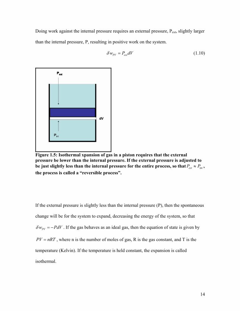
Doing work against the internal pressure requires an external pressure, Pext, slightly larger

than the internal pressure, P, resulting in positive work on the system.

PV extw P dV (1.10)

Figure 1.5: Isothermal xpansion of gas in a piston requires that the external pressure be lower than the internal pressure. If the external pressure is adjusted to be just slightly less than the internal pressure for the entire process, so that intextP P , the process is called a �“reversible process�”. If the external pressure is slightly less than the internal pressure (P), then the spontaneous

change will be for the system to expand, decreasing the energy of the system, so that

PVw PdV . If the gas behaves as an ideal gas, then the equation of state is given by

, where n is the number of moles of gas, R is the gas constant, and T is the

temperature (Kelvin). If the temperature is held constant, the expansion is called

isothermal.

PV nRT

14

d) Electrical work (Figure 1.6): The work of moving a charge, Q, by a distance dx, in an

electrostatic potential, is given by

( )elw d Q (1.11)

A negative charge will move spontaneously towards a more positive potential, in which

case the work done is negative since the potential energy is decreased, i.e., if Q<0 and

>0, then d 0elw .

Figure 1.6: The negative electric potential from the charged surface is a measure of how much work is required to move a charge near the surface. The potential energy decreases as a positive charge gets closer to the negative surface. Positive work is required to move the positive charge away from the negative surface. We will consider later the work of moving ions across membranes or to move a charged

substrate near a charged surface of a protein, membrane or polynucleotide, for example.

The work of moving an ion from the aqueous medium to the inside of a protein or to the

inside of a membrane is more complicated because the medium changes.

e) Moving an object in a centrifugal force field (Figure 1.7): This will be

encountered when we consider how molecules behave in a centrifuge.

2centf m r (1.12)

(1.13) 2( )centw m r dr

15

where m is the mass of the molecule (which we need to adjust for buoyancy), is the

circular velocity of the rotor (radians/sec) and r is the distance from the center of the

centrifuge rotor to the location of the molecule in the centrifuge tube. As the particle

sediments under the influence of the centrifugal force, its potential energy is decreased

and the work is negative.

Figure 1.7: The centrifugal force on a particle in a spinning centrifuge tube drives the particle away from the center of rotation. As the particle is displaced, the potential energy decreases. BOX 1.2 Differential changes and integration

It is often more convenient to functional relationships in differential form, as in

equations(1.8), (1.9) or (1.10), for example In asking what work is required to move a

particle which is at a particular position, x1, by an infinitesimally small amount, dx, the

force can be considered to be constant between positions x1 and the new position (x1 +

dx): 1 1( ) ( )f x f x dx . If we want to compute the amount of work in going from one

16

position ,x1, to another position, x2, we can sum up the w values for each step. This is

illustrated in Figure 1.8, which schematically shows the plots of force vs position for

lifting a weight (gravity), stretching a spring, expanding an ideal gas, and centrifugation

of a particle. In each case, ( )w f x dx , and we can break up the displacement from

the starting position (�“1�”) to the final position (�“2�”) into a sequence of small,

infinitesimal steps (dx, dV or dr). Note that the expression for the work at each step is

equal to the area of the rectangle between x and x+dx (shaded in Figure 1.7). Hence,

summing up the work accomplished in each step between the defined limits (position 1 to

position 2) is equivalent to evaluating the area under the curve defined by f(x) vs x.

Figure 1.8: Four examples of the work done by displacing an object in the presence of a force. In each case the process is taken in small steps, and after each step the system re-equilibrates. In the examples of lifting an object or stretching a spring, an external applied force is used to do work on the object (positive work). In these examples, the applied force is just slightly larger than the force tending to restore the system towards equilibrium. For the isothermal expansion of an ideal gas the external pressure is adjusted to be just slightly less than the pressure within the piston and negative work is done by the gas in the piston. For the centrifugation of a particle, the force displaces the particle towards the bottom of the tube. Note that work is expressed as the area underneath each curve between the initial and final limits.

17

In each example, asides from gravity, the value of the force, and therefore the work for

each infinitesimal step, changes with position. The area under each curve is given by the

integral of f(x) between the defined limits. In these examples we can relate the integrals

to the amount of work done.

a) lifting a weight: 2

1

2 1( )x

x

w mgdx mg x x

b)stretching a spring: 2

2

11

2 22 1

1 1 ( )2 2

xx

S S Sxx

w k xdx k x k x x2

c)isothermal expansion of an ideal gas: 2 2

1 1

1

2

( ) ln(V V

V V

VnRTw PdV dV nRTV V

)

d) centrifugation of a particle: 2

2

11

2 2 2 2 21 2

1 1 ( )2 2

rr

rr

w rdr r r r2

h

END BOX

1.3 Equilibrium and the extremum principle of minimal energy: a ball in a

parabolic well.

Consider a ball placed in a two-dimensional well, as pictured in Figure 1.9. The

gravitational potential energy is given by

( )potU h mg (1.14)

where m is the mass of the ball, g is the gravitational acceleration constant and h is the

height. If the well has a parabolic shape, then h = x2 and we can write

(1.15) 2( )potU x mgx

18

We know that the ball will roll within the well until it reaches a point of minimal

potential energy. This is an example of an �“extremum principle�”.

Figure 1.9: Potential energy of a ball in a potential energy well created by a parabolic shaped container in which the ball is under the influence of gravity.

The location of minimal potential energy in this case is clearly the bottom of the well,

where xeq = 0. We can obtain this by looking at Figure 1.8, and observing that at the

minimal value of the potential energy, the slope of the tangent to the curve is zero

(horizontal). In other words, the first derivative of Upot(x) with respect to x is zero.

Taking the derivative of equation (1.15) and setting it equal to zero gives

( )

2potdU xmgx

dx0 (1.16)

which is satisfied when x = 0. This defines the equilibrium position, which is where

xeq = 0.

The force on the ball is defined as the negative of the gradient or first derivative

of the potential energy, Upot(x), with respect to position (x) as in equation(1.1). The

19

larger the magnitude of the change in potential energy for a small displacement of the

position (dx), means there is a larger driving force towards restoring the equilibrium

position (x = 0). This is pictured in Figure 1.9. Displacement to the left of xeq results in a

force that is positive, driving the ball to values of increasing values of x. Displacement to

positive values of x, away from xeq results in a negative force, driving the ball to the left.

The force, by definition, drives the ball to decreasing values of the potential energy until

the minimum is reached, at which point the force is equal to zero.

We can also define the position of equilibrium as the point where the force f = 0,

since the minimum of the potential energy, equation (1.16), is identical to the condition

where the net force is zero.

( ) ( )

at equilibrium, 0 pot potdU x dU xforce

dx dx (1.17)

The force on the ball is larger as it gets further from the equilibrium position, and the

tendency is for the ball to roll from a position of higher potential energy to one of lower

potential energy. The force quantifies the tendency of the ball to roll towards its

equilibrium position, defining both the magnitude of the tendency and also the direction.

The equilibrium position is the configuration that the system tends towards

spontaneously. For a ball at the bottom of the gravitational potential well, a displacement

of the ball in either direction from its equilibrium position will result in a force that will

tend to bring the ball back to the equilibrium position. Mathematically, the statement that

the equilibrium position is a minimum in potential energy (as opposed to a maximum,

where the force would also be zero) means that the second derivative of the potential has

a positive value.

20

2

2

( )0 at pot

eq

d U xx x

dx (1.18)

Another useful concept we can illustrate from this model is the principle of the

conservation of energy. If we place the ball near the top of the well, it starts with a given

amount of potential energy ( )potU h mgh . By picking up the ball and placing it at this

position, we have done work against gravity which has been conserved as potential

energy. When we let go of the ball, it rolls under the force of gravity, picking up kinetic

energy. At the bottom of the well, the potential energy has been converted entirely to

kinetic energy, if there is no loss due to frictional forces. The ball would oscillate back

and forth forever were it not for the conversion of some of its kinetic energy to heat due

to friction encountered with the surface of the well in which it is rolling. The ball and

well are in thermal contact with the surroundings and the heat is lost to the environment.

Eventually, all the potential energy that we started with at the top of the well is converted

to heat and the ball will come to rest at the equilibrium position.

This simple example contains the essence of what we want to obtain from

thermodynamics. We will be defining potentials which will tell us how energy will flow

in the form of work and heat, how material will move from one place to another, and how

chemical reactions will proceed in biological systems as they undergo changes from an

initial set of conditions towards equilibrium.

It is reasonable to ask why a mechanical description is not sufficient to describe

work done in biochemical systems. If you pick up a weight the potential energy of the

weight is increased by a known amount, and you can calculate how much work you can

do with this weight as it is lowered back to the ground. If you hydrolyze ATP to ADP and

Pi there is also a well-defined bond energy for the hydrolysis of the so-called �“high

21

energy�” bond. However, unlike the mechanical system, this information is insufficient to

tell us how much work we can get out of this reaction. If we have large concentrations of

ADP and Pi and a small concentration of ATP, then we cannot get any work out of the

system, whereas, if we hydrolyze the same number of ATP molecules in a solution with a

high concentration of ATP and low concentrations of ADP and Pi, we can get work out of

the system. There is something else going on besides what we can see by considering the

bond energies of the molecules. Thermodynamics tells us what this additional factor is

and how it can be quantified. Thermodynamics is of central importance in understanding

biochemical and chemical processes.

BOX 1.3 A word about units

Throughout this text, the Standard International (SI) system of units will be used. This is

the modern version of the metric system. There are 7 SI base units: 1) kilogram (mass);

2) meter (length); 3) second (time); 4) thermodynamic temperature (kelvin); 5) electric

current (ampere); 6) mole (substance); 7) candela (luminous intensity). All other units

follow from these. Most important for our purposes is the unit of energy, the joule, named

after James Prescott Joule. The joule is defined as the work expended to move an object

one meter using a force of 1 Newton. A Newton is the amount of force required to

accelerate a mass of 1 kilogram at a rate of one meter per second squared.

2

2

1 1

1 1

J Nm

mJ kgs

A joule is also the amount of energy required to move an electric charge of 1 coulomb

through an electrical potential difference of 1 volt. If you drop this textbook to the floor,

the amount of energy lost is about 1 joule.

22

Energy is still often reported using the unit of the calorie (or kilocalorie). The

calorie is approximately the amount of energy needed to raise the temperature of 1 gram

of water by 1oC (at 15oC).

1 calorie = 4.186 joules

1 joule = 0.239 cal

END BOX

1.4 From one to many: The Principle of Maximal Multiplicity

The trek from a mechanical system, like a spring or a ball in a well, to metabolic

reactions and active transport systems requires that we first realize that in studying

biological or chemical systems we are dealing with the collective behavior of a large

number of molecules. A cell that is about 10µm in diameter containing 1 mM ATP

contains about 1 billion molecules of ATP. Many years of experiment and observation

has provided us with a remarkably powerful principle that allows us to predict the

behavior of a large collection of molecules. This is the Principle of Maximal

Multiplicity which, as we will see, is a statement of the Second Law of

Thermodynamics.

The Principle of Maximal Multiplicity states that in any system of many particles

that is isolated from its surroundings, the system will tend towards an equilibrium which

has the largest number of equivalent microscopic states. This statement, plus the

recognition of the equivalence of work and heat (the First Law of Thermodynamics) are

sufficient to derive all of thermodynamics, which includes a quantitative description of

the driving forces that determine the behavior of chemical and biochemical systems.

23

Probabilities and Microscopic States: To see what is meant by equivalent microscopic

states, let�’s look at a simple system. In the system pictured in Figure 1.10, there are 4

particles. The energy of each particle is quantized and can take on values of 0, 1, 2, 3 or

4, and we will assume that the particles can exchange energy so each of the particles

might have any of the allowed energies (0, 1, 2, 3 or 4). Now, we will constrain the total

energy, U, to be 4 units. There are 35 distinct combinations where the total energy is

distributed among the 4 particles to yield this total (Figure 1.10). We can define a

variable, W, as the multiplicity of a system. In this example, W = 35. These microscopic

states can be assigned to one of five distinct configurations.

i) Any one of the four particles can have an = 4 while the other three = 0.

There are four different arrangements.

ii) Any one of the four particles can have = 3, and another = 1 with the

remaining two having = 0. There are 12 distinct arrangements.

iii) Any two particles can have = 2 and the remaining two particles each have

= 0. There are 6 distinct arrangements.

iv) Any two particles can have = 1 and one other particle have = 2. There are

12 distinct arrangements.

v) All the particles can have = 1. There is only one such arrangement.

24

Figure 1.10: There are five different energy configurations and 35 equivalent microscopic states in which a total of 4 energy units is distributed among 4 indistinguishable particles, in which each particle is allowed to have an energy of 0, 1, 2, 3 or 4 energy units. Each card represents a distinct microscopic state.

Each of these 35 microscopic states is consistent with the macroscopic constraint on the

total energy. The Principle of Maximal Multiplicity simply states that at equilibrium each

of the 35 microscopic states is equally likely to be present at any instant in time. This is

common sense. We might initially add to our box one particle with = 4 and three

particles with = 0, but we are very unlikely to find this distribution of energy among the

particles after letting them equilibrate. Equilibration implies that there is some

mechanism by which the energy can be redistributed among the particles. For molecules,

this mechanism would be by collisions. We cannot know with certainty the distribution

25

we will find at any instant. All we can do is compute the probabilities of finding

particular microscopic states. For example, 12 of the 35 microscopic states have one

particle with = 3, so in this set of 12 states, the probability of finding a particle with =

3 is 0.25. In the other four configurations (Figure 1.10), the probability of finding a

particle with = 3 is 0.0. Hence, over all 35 microscopic states, the probability of

finding a particle with = 3 is the weighted average over the three configurations.

312 1 4 12 6(0) (0) (0) (0.25) (0) 0.08635 35 35 35 35

p

Similarly, the probabilities of finding a particle with energies of 4, 2, 1 and 0 energy are

readily determined at equilibrium, using the criterion that each microscopic state is

equally probable.

112 1 4 12 6(0.5) (1.0) (0) (0.25) (0) 0.2835 35 35 35 35

p

212 1 4 12 6(0.25) (0) (0) (0) (0.5) 0.1735 35 35 35 35

p

412 1 4 12 6(0) (0) (0.25) (0) (0) 0.02835 35 35 35 35

p

012 1 4 12 6(0.25) (0) (0.75) (0.5) (0.5) 0.4335 35 35 35 35

p

In the case of the single ball in a parabolic well, if we have no frictional loss of energy,

then the total energy of the ball (potential plus kinetic energy) remains constant and is

exactly defined. If the energy is divided among a number of particles, as in the current

example, the total energy is consistent with many equivalent microscopic states. With a

small number of particles, as in this example, we can easily count the number of

microscopic states consistent with the macroscopic constraints of energy and particle

26

number (total energy, U = 4 and number of particles, n = 4, in this example). When we

have a large number of indistinguishable particles (or molecules), we cannot literally

count microscopic states to arrive at the value for the multiplicity (W), but the same

Principle of Maximal Multiplicity applies and defines how energy is distributed among

the particles at equilibrium.

1.5 Entropy and the Principle of Maximal Multiplicity: Boltzmann�’s Law

Multiplicity is a fundamental property of any system, and is determined by the

way in which energy and material is dispersed. In any isolated system the energy and

material within the system will evolve spontaneously from any starting point to maximize

the multiplicity, W, at which point the system is in equilibrium. It was Ludwig

Boltzmann, in the later half of the 19th century, who recognized the fundamental

importance of multiplicity, and he defined Entropy, S, as the functional form that would

be most useful.

ln( )S k W (1.19)

where k is Boltzmann�’s constant and has a value of 1.380662 x 10-23 JK-1. Since

maximizing W will also maximize ln(W), an isolated system at equilibrium can be

defined as having the maximum entropy. The units and value of Boltzmann�’s constant

are defined to fit into the framework of thermodynamics as it had been previously

established. This is described in the next Section.

The definition of entropy in equation (1.19) has a drawback insofar as it involves

counting up microscopic states of a system to get W. Clearly, this is not practical for most

27

problems of interest. An alternative definition that is mathematically equivalent for a

system with a large number of possible configurations is

1

lnn

ii

S p pk i (1.20)

where ip is the probability of the system being in a particular configuration. We will not

derive this form of the equation, which can be found in Dill and Bromberg. For the

example in Figure 1.10, with 4 particles, the five possible energy distributions are

{4,0,0,0}, {3,1,0,0}, {2, 1, 1, 0}, {1, 1, 1, 1} and {2, 2, 0, 0}with probabilities of

4 12 6 1 120.11, 0.34, 0.17, 0.03 and 0.3435 35 35 35 35

, respectively. However, the

number of configurations is too small for equation (1.20) to be valid.

Figure 1.11: The increase in entropy for a simple situation of bringing two systems together. System A has 2 particles and 2 units of energy. Each particle can have either 0 or 1 unit of energy. System B has only 4 particles but also has 2 units of energy. The multiplicity of the two systems considered together ( )is the product of the multiplicity of the two separate systems. The numerical solution to the number of equivalent systems is given, where

, and there are 270 equivalent ways to arrange identical particles in this manner. If the systems are brought into contact and one energy unit is allowed to move from the small system (B) to the larger system (A), the multiplicity increases to 480. This shows that this process would be spontaneous since the energy flow in this direction results in increasing the entropy.

AW WB

N"N factorial" = ! (1)(2)(3)...( 1)( )N N

28

As an example, let�’s say that we start with two separate systems, each at

equilibrium. The larger system (A) has 10 particles with a total of 2 energy units, and we

will allow each particle to have an energy of either 0 or 1 unit. The smaller system (B)

has only 4 particles but also an energy of 2 units (see Figure 1.11). System A has 45

equivalent states and system B has 6 equivalent states. Hence, the two systems together

have 45(6) = 270 equivlalent states. We will now bring these two systems into contact

and allow energy to exchange. Without worrying about the final equilibrium state, which

would maximize the multiplicity, we will simply ask if it is favorable for one unit of

energy to flow from the small to the large system, pictured on the right side of Figure

1.11. There are now 120 equivalent microscopic states for system A and 4 for system B.

The total multiplicity is now (120)(4) = 480, which is higher than the initial energy

distribution. Redistribution of energy in this simple model system can be seen to increase

the multiplicity, and, hence, this would be a spontaneous process towards equilibrium.

Energy flow in the opposite direction (form the large system to the small system)

decreases the multiplicity and, would not occur spontaneously.

The equilibrium condition for an isolated system, in which no energy or matter

can enter or leave (in this example, the combination of systems A + system B is isolated

from the surroundings), is that entropy is maximized. It is important to emphasize that the

principle of maximizing entropy applies to isolated systems, meaning that the energy and

material within the system is fixed. We will soon see how to apply this principle to

biological or chemical systems where this constraint does not apply. Before we do this,

however, we need to introduce additional concepts in thermodynamics, out of which will

29

come another definition of entropy (Section 1.16) providing further insight into the

meaning of entropy as well as the means to measure entropy experimentally.

Our goal is to end up with a potential function, analogous to potential energy in a

mechanical system, that can be used to quantify the driving force for biochemical

processes and also to quantify how much work can be obtained from such processes.

1.6 Thermodynamic Systems and Boundaries

The universality of thermodynamics can also make this subject appear very dry

and disembodied from familiar objects of interest, and the language is necessarily very

general. We will start by defining a thermodynamic system. If we want to examine

what goes on within a biological cell, for example, we need to first consider what goes

into or out of the cell. It is useful, therefore, to differentiate the object to be studied, a cell

in this case, from everything else. A thermodynamic system can be defined as anything

you are interested to examine, separated from the rest of the universe, or surroundings

by an imagined or real boundary.

Figure 1.12: A thermodynamic system is whatever you are interested in examining, separated from the rest of the universe (the surroundings) by a real or imagined boundary.

For example, a system could be a bacterial cell, the contents of a flask, a pulley with

weights, a steel ball in a well or even yourself or the entire earth(Figure 1.12). A

30

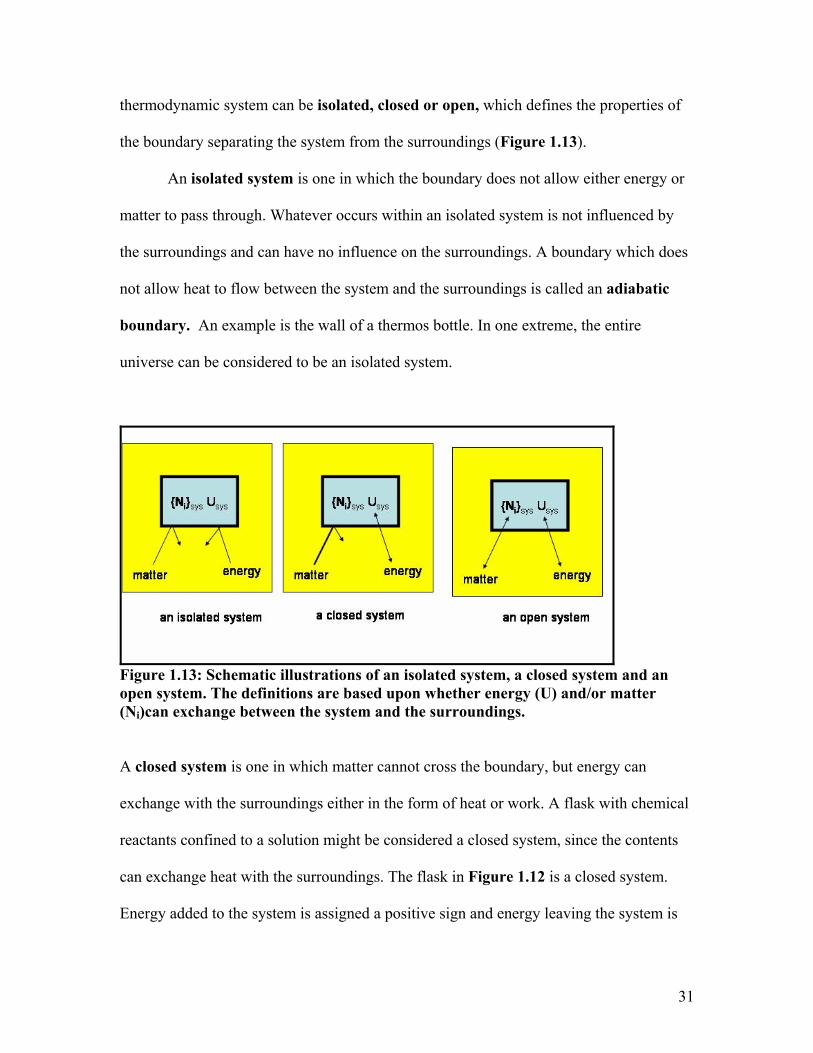
thermodynamic system can be isolated, closed or open, which defines the properties of

the boundary separating the system from the surroundings (Figure 1.13).

An isolated system is one in which the boundary does not allow either energy or

matter to pass through. Whatever occurs within an isolated system is not influenced by

the surroundings and can have no influence on the surroundings. A boundary which does

not allow heat to flow between the system and the surroundings is called an adiabatic

boundary. An example is the wall of a thermos bottle. In one extreme, the entire

universe can be considered to be an isolated system.

Figure 1.13: Schematic illustrations of an isolated system, a closed system and an open system. The definitions are based upon whether energy (U) and/or matter (Ni)can exchange between the system and the surroundings.

A closed system is one in which matter cannot cross the boundary, but energy can

exchange with the surroundings either in the form of heat or work. A flask with chemical

reactants confined to a solution might be considered a closed system, since the contents

can exchange heat with the surroundings. The flask in Figure 1.12 is a closed system.

Energy added to the system is assigned a positive sign and energy leaving the system is

31

given a negative sign (see Figure 1.14), analogous to adding or subtracting from the

potential energy in mechanical systems.

Figure 1.14: The sign convention for energy exchange between a system and its surroundings. Energy leaving the system is negative because it reduces the amount of energy in the system. Energy added to the system is considered positive. The same convention applies to matter exchanged between the system and surroundings.

An open system is one in which both matter and energy can cross the boundary which

separates the system from the surroundings. If material were able to exchange between

the flask pictured in Figure 1.14 and the surroundings, for example by evaporation and

condensation, this would be an open system. Material entering the system from the

outside is given a positive sign and material leaving is given a negative sign. The signs

denote the changes in the amount of material or energy within the system.

Living organisms are open systems. Open systems can be separated from the

surroundings by boundary that is semipermeable, allowing certain molecules to pass

through but not others. This is a property of biological membranes.

32

Figure 1.15: The nucleus and mitochrondrion can be considered as subsystems of the cell, which itself can be considered to be a thermodynamic system. In these cases the thermodynamic boundaries are equivalent to the semipermeable membranes surrounding each system, allowing certain molecules to pass ({Ni})as well as allowing heat (q)to exchange

Any system can contain subsystems which are mechanically separated from each other

and which can exchange matter and/or energy. The mitochondrion can be considered to

be a subsystem within a cell, for example (Figure 1.15).

1.7 Characterizing the System: State Functions

Once a system has been defined, the state of that system is characterized by State

Functions or State Variables. The most obvious functions are temperature (T), pressure

(P), volume (V) and material composition ({Ni}). The material composition and volume

are extensive functions, meaning that their magnitudes are proportional to the size of the

33

system. In contrast, temperature and pressure are intensive functions, and do not vary in

proportion to the size of the system (Figure 1.16).

Figure 1.16: Extensive variables are additive when considering multiple systems, and include volume (V), the number of particles {Ni}), internal energy (U) and entropy (S). Note that material and energy are not allowed to pass between systems. Intensive variables do not change with the size of the system, and include temperature (T) and pressure (P). In this case, the temperature and pressure are the same for both systems 1 and 2.

Thermodynamics introduces two additional extensive state functions that are of

fundamental importance: internal energy (U) and entropy (S). Internal energy is the

sum of the kinetic and potential energies of each of the components of the system.

Boltzmann�’s statistical definition of entropy in terms of multiplicity or probabilities of

equivalent microscopic states, equation (1.20), was added after the formulation of

thermodynamics, but is fully compatible with the initial thermodynamic definition of

entropy, which we will encounter in Section 1.16. Basically, internal energy defines how

much energy is present in the system and entropy expresses how the energy is dispersed

among the components at equilibrium.

34

The thermodynamic state of any system is completely defined by the values of

the extensive functions: volume, material composition, internal energy and entropy (V,

Ni, U and S). Furthermore, if V, N and U are fixed, then the value of S is determined,

assuming the system is at equilibrium. We saw this in the simple model in Figure 1.10,

in which the entropy at equilibrium is defined given the internal energy and number of

particles. Hence, there must be some function of V, N and U that defines S at

equilibrium.

( , , )S S V N U (1.21)

Under some circumstances, the internal energy and entropy of a system can be measured

and given numerical values. However, in most cases, the absolute values of internal

energy (Joules) and entropy (Joules K-1) are not readily evaluated, as are, for example

temperature or the concentrations of components. Nevertheless, internal energy and

entropy are at the heart of the First and Second Laws of Thermodynamics. Before we get

to that, we need to discuss what we mean by heat and internal energy and then take

another look at the concept of entropy. We will then arrive at formulations of

thermodynamics that are suited to solve everyday problems of interest to biologists and

chemists, using readily measured properties.

1.8 Heat

We all have an intuitive knowledge of heat, which is designated as q. When a hot

object is brought in contact with a cold object, we speak of heat flowing from the hot to

the cold object. Indeed, for many years, heat was considered to be a fluid substance with

mass (Caloric Theory) and was thought to be conserved. However, heat has no mass, and

35

is neither a fluid nor is it conserved. If you rub two sticks together, they get hot (at least if

you are a boy scout), so work can be converted to heat.

Heat (q) is a concept that is inseparable from the process of the transfer of energy

(U). We now know that in molecular terms, the energy is transferred in terms of the

thermal motions of molecules of the hot object stimulating the increase in thermal motion

of molecules in the cold object. Hence, the transfer of heat from a hot to a cold object

results in decreasing the internal energy of the hot object and increasing the internal

energy of the cold object. We know from experience that at equilibrium the temperatures

of each of the two objects will be identical. Note that if we have a large cold object and a

small hot object, energy in the form of heat will be transferred from the hot to the cold

object even though, in quantitative terms the internal energy of the cold object, because

of its large size, may be much larger than that of the hot object. Equilibration does not

result in an equal distribution of internal energies between the objects in contact.

Consider the example in Figure 1.17 in which we have two subsystems within an

isolated system. The two subsystems are combined and heat is allowed to pass between

the two subsystems, but neither the distribution of matter nor the volumes change. We

start with a situation where the object comprising System 1 is at a lower temperature but

is much larger than the object comprising System 2. When they merge, heat (q) is

transferred from the smaller, hotter object to the larger, colder object. The total internal

energy (U1 + U2) remains constant, as do the total number of molecules (N1 + N2) and the

36

Figure 1.17: Two subsystems are combined and heat is allowed to transfer between them. At equilibrium, the entropy of the combined system, which is isolated from its surroundings, will be maximal. Maximizing the entropy leads to the conclusion that the temperatures of each system in thermal contact will be identical at equilibrium. The redistribution of energy leads to the increase in entropy as the combined systems attain a new equilibrium.

total volume (V1 +V2). However, the distribution of energy has been altered and, thus S1

and S2 change. The total entropy of the isolated, combined systems, will increase as heat

flows, and will reach a maximal value at equilibrium. At equilibrium the only

consideration is the multiplicity of microscopic states is maximal and all possible

microscopic states are equally likely.

A chemical process, such as the hydrolysis of ATP, that releases energy in the

form of heat is an exothermic process. In an isolated system, this usually results in

increasing the temperature of the system. In an open system, such as in a cell or test tube,

the heat is transferred to the surroundings to maintain constant temperature at

equilibrium. Heat leaving the system is assigned a negative sign. A process in which heat

is acquired from the surroundings in an open system is called an endothermic process

(see Figure 1.18). If an endothermic process occurs within an isolated system, we expect

the temperature to decrease.

37

Figure 1.18: Endothermic and exothermic processes are illustrated by biochemical reactions in a test tube. An exothermic process generates heat which, in system in thermal isolation from the surroundings, generally results in an increase in temperature or, in a system in thermal contact with the surroundings, transfers heat to the surroundings. If the surroundings is very large (here pictured as a large water bath), the heat will not have a measurable influence on the temperature and the entire process is maintained at constant temperature (an �“isothermal�” process). In an endothermic process, heat is taken up from the surroundings, if the system is in thermal contact. If not, the temperature decreases. Heat is measured in units of calories or joules. A calorie (small calorie or gram-

calorie) is defined as the amount of heat needed to increase the temperature of 1 gram of

water by 1oC, from 14.5oC to 15.5 oC. This is equal to 4.184 joules in SI units.

Since biological systems are open systems, exothermic and endothermic processes

result in the transfer of heat either to the surroundings (exothermic, q<0), or take heat

from the surroundings (endothermic, q>0). If the surroundings are large enough to

acquire or release heat without changing temperature, then this also will also maintain the

temperature of any system equilibrated with the surroundings at the same, constant

temperature. A process that occurs at constant temperature is called an isothermal

processes. When the surroundings are considered unperturbed by the transfer of heat to or

from it, this is referred to as a heat �“reservoir�”.

38

1.9 Pathway-independent functions and thermodynamic cycles.

The state of a system is defined by the values of state variables. If we define two

states of a system, State 1 (T1, P1,V1, N1, U1and S1) and State 2 (T2, P2,V2, N2 U2and S2),

the net change in the state variables if we go from State 1 State 2, do not depend on

the mechanism of the process, the order of events, or the nature of intermediate states

passed through along the way. The changes in the state variable are pathway-

independent. In the schematic in Figure 1.19, we consider that the temperature, pressure

and composition of the system is altered to go from State 1 to State 2.

Figure 1.19: Two different pathways leading from State 1 to State 2 (red and green arrows Pathway 1 3 4 5 2 1 is a thermodynamic cycle ( red arrows). It does not matter if we heat it before or after changing the composition or changing the

pressure, or if we heat it last. The final state remains the same and the net changes in the

state variables (e.g., S = (S2 �– S1), U = (U2 �– U1) etc) do not depend on the pathway

39

but only on the final and initial state. In the special case in which our sequence of

processes (the pathway) brings us back to the initial state of the system, then there is no

change in the values of the state variables, (e.g., S = U = 0, etc). This is called a

thermodynamic cycle, and one is included in Figure 1.18. Once we realize which

variables are state variables, the simple concept of pathway-independence has a great

practical value in calculating the values of thermodynamic parameters, as we will see.

1.10 Heat and work are not state variables

It is particularly important to realize which variables are state variables and which

are not state variables. The example of obtaining work by lowering (or dropping) a

weight on a pulley (Figure 3) illustrates three different ways of going from an intitial to a

final state in which different amounts of work and heat are generated in each pathway. To

emphasize this point, let�’s look at another example in which we focus on the potential

energy of a box filled with lead weights (Figure 1.20). Since there is no kinetic energy,

the total energy is equal to the potential energy in a gravitational field. We can define

State 1 as the Box on the ground floor of a building and State 2 as the box on the second

floor. The potential energy is defined entirely by the position of the box and not on how it

got to this position. This is what is meant by pathway independence of the internal

energy, which is a state function.

We need to do work to move the box from State 1 State 2. The simplest

pathway is to simply carry the box up one flight of steps and put it down. However, we

might carry the box up to the third floor and, realizing our mistake, and out of frustration

just drop it down to the second floor. When the box hits the floor it will generate heat

from the kinetic energy it has picked up as it falls. By carrying the box an extra flight of

40

stairs, we are doing more work on the box, and that extra work is then lost to the

environment as heat after we drop the box. The potential energy of the box is the same

by either pathway, but both work and heat depend on the pathway. Work and heat are not

state functions.

Figure 1.20: Two pathways used to move a box of lead weights from the first to second floor. Energy (U) is a state function, whereas each of the two pathways involves a different amount of work and heat, which are not state functions.

The fact that heat and work are not state functions is signified by expressing differential

changes in work or heat as w and q instead of dw and dq, since their magnitude will

depend on the pathway used for the displacement. The differential changes in state

functions, such as internal energy and entropy will be designated by dU and dS, to

indicate that these are exact values and not dependent on the pathway of the change in the

system.

Now we are in a position to discuss the First Law of Thermodynamics.

1.11 Internal Energy (U) and the First Law of Thermodynamics

41

The First Law of thermodynamics states that work and heat are equivalent, and

that the internal energy of any system can be altered only by an exchange of either work

(w) or heat (q) with the surroundings.

U q w or dU q w (1.22)

When heat is transferred, the random motion of the molecules is stimulated, whereas the

transfer of energy in the form of work stimulates a uniform movement of the molecules

(such as moving an object).

In a transition from State 1 State 2, the difference in internal energy

2 �–U U U1 (1.23)

is fixed, but any combination of work and heat that is consistent with this value might be

used in the transition. The convention is that work or heat transferred into the system

from the surroundings is defined as positive (+q, +w), whereas when work or heat is

transferred from the system to the surroundings, the sign is negative, (-q, -w) (Figure

1.14).

This first law implies that in any isolated system the internal energy must remain

constant, since no work or heat is allowed through the system boundary. If we consider

the entire universe to be an isolated system, then the first law states that the total energy

in the universe is a constant and, therefore, energy can be neither destroyed nor created.

1.12 Measuring U for processes in which no work is done

If we simply heat a system and keep the volume constant, then there can be no PV

work ( ). In the absence of any other kind of work (0PVw 0)nonPVw �’ then and,

since , the change in the internal energy is simply equal to the heat transferred

0w

U q w

(1.24) where the subscript indicates constant volume.VU q

42

Hence, we have a method, under limited circumstances, to measure U. If we have a

uniform substance, the amount of heat necessary to raise the temperature by 1K under

conditions of constant volume, is CV (units JK-1).

V Vq C dT (1.25)

Therefore,

VdU C dT (1.26)

If CV is a constant, i.e., does not vary as the temperature of the system is changed, then

we can determine the change in internal energy in heating the substance from T1 to T2, by

simple integration

(1.27) 2 2

1 1

U T

VU T

dU C dT

(1.28) 2 1 2 1( ) (VU U U C T T )

V

So, if we heat a system that is held at constant volume, all the heat goes into increasing

the internal energy of the system. However, most biological processes don�’t occur at

constant volume, but rather at constant pressure.

1.13 Enthalpy and heat at constant pressure

Most of the systems we will be studying are open to the atmosphere and,

therefore, processes are measured at constant pressure (an external pressure, Pext = 1 bar).

If we heat a substance that is open to the atmosphere, then it is possible that there will be

a change in volume (dV) and, therefore, some of the energy added as heat to the system

will be used to do work against the atmospheric pressure, PV extw P d , where the

negative sign indicates work done by the system on the environment (dV>0 for an

expansion). If no other work is allowed ( 0nonPVw ), then we can write

43

P extdU q w q P dV (1.29)

where the subscript indicates that the heat is delivered under conditions of constant

pressure. This expression can be rearranged to yield

PdU PdV q (1.30)

where the �“ext�” subscript has been dropped for convenience.

Since pressure is constant, dP = 0, so we can add a VdP term to equation to get

( ) (Pq dU PdV VdP d U PV ) (1.31)

The amount of heat ( Pq ) released or taken up during a process, such as a biochemical

reaction, at constant pressure, can be experimentally measured using a calorimeter. For

this reason the thermodynamic expression on the right hand side of equation (1.31) is

given a special name, enthalpy, H.

H U PV (1.32)

dH dU PdV VdP (1.33)

It is only for a process where the pressure is the same in the initial and final states

( ) that we can write 0dP

dH dU PdV (1.34)

Note that since U, P and V are state functions, enthalpy is also a state function.

The amount of heat needed to raise the temperature of a substance by 1K at constant

pressure is equal to CP, the heat capacity at constant pressure (units JK-1). Hence,

P Pq C dT (1.35)

PdH C dT (1.36)

44

The numerical value of CP will depend on the pressure under which the measurement is

made. Under conditions where CP at a defined pressure is constant and does not vary with

temperature, we can write

2 1(PH C T T ) (1.37)

When a system is heated at constant pressure, e.g., maintained at atmospheric pressure,

some of the heat goes to increase the internal energy and some of the heat is used to do

work on the atmosphere if the system expands. Enthalpy accounts for both of these

consequences

More pertinent is the release or uptake of heat during chemical or biochemical reactions

that take place at constant pressure. The change in enthalpy of a system under these

conditions is due to the making and breaking of chemical bonds. Since the amount of

PV work is usually small in biochemical processes, the changes in enthalpy and internal

energy are usually about the same.

1.14 The caloric content of foods: reaction enthalpy of combustion

When one refers to the energy content of a food, this generally refers to the

amount of heat released upon combustion to yield CO2 and H2O. For example, for

sucrose, the combustion reaction is

(1.38) 12 22 11 2 2 2C H O (s) + 12 O ( ) 12 CO (g) 11 H O (l)g

where the (s), (g) and (l) refer to the solid, gaseous and liquid state. The oxidation of

sucrose also occurs in the human body, though fortunately not in a simple combustion

reaction, but through a series of many enzyme-catalyzed steps. As far back as 1780,

Lavoisier and LaPlace demonstrated that the heat produced by mammals is the same as

the heat generated upon the combustion of organic substances, and that the same amount

45

of O2 is consumed. (Kleiber M. 1975. The Fire of Life. An Introduction to Animal

Energetics. New York: Robert E. Krieger Publishing; Holmes FL. 1985. Lavoisier and

the Chemistry of Life. Madison, WI: University of Wisconsin Press.). Since enthalpy (H)

is state function, the change in enthalpy due to the oxidation of sucrose to CO2 and H2O

will be exactly the same regardless of the pathway between the initial and final states.

Hence, the value of H measured in a one-step combustion reaction is the same as that

resulting from the biological pathway, consisting of many steps, but leading to the same

products.

For the combustion of sucrose, the initial state can be defined as 1 mole of solid

sucrose plus 12 moles of O2 gas and 298.15K and 1 bar pressure, and the final state is 12

moles of CO2 gas and 11 moles of liquid water, also at 298.15K and 1 bar pressure. The

choice of 298.15K and 1 bar pressure is usually taken as a �“standard state�” as a matter of

convenience.

Each of the reactants and products has absolute values for its internal energy and

enthalpy under the conditions of the standard state, and we can denote these as

etc. where the subscript �“m�” indicates the value per

mole and the superscript �“o�” indicates the standard state (298.15K and 1 bar). We can

now define the reaction energy and reaction enthalpy

o om 12 22 11 m 12 22 11U (C H O ,s), H (C H O ,s)

or mU o

r mH for the reaction

describing the combustion of sucrose.

(1.39)

0 02 2 12 22 11 2

0 02 2 12 22 11 2

12 ( , ) 11 ( , ) ( , ) 12 ( , )

12 ( , ) 11 ( , ) ( , ) 12 ( , )

o or m m m m m

o or m m m m m

U U CO g U H O l U C H O s U O g

H H CO g H H O l H C H O s H O

o

o g

46

These are the molar reaction energy, ,and the molar reaction enthalpy,or mU o

r mH . Note

that the �“molar�” means per mole as the reaction as it is written, normalized to 1 mole of a

particular reactant or product. If we divided every term by 12 to normalize the reaction to

one mole of CO2, the values of would be divided by 12. and or m r mU oH

Experimentally, the heat of this reaction must be measured using a bomb

calorimeter (Figure 1.21), because gases are involved and it is necessary from a practical

viewpoint to do the reaction in a sealed vessel at constant volume.

The heat released at constant volume in the reaction container is transferred by

equilibration to a large water bath and measured by the increase in temperature of the

water. Since a large mass of water is used, the temperature of the reaction system itself is

maintained at approximately the same temperature (298.15K).

47

Figure 1.21: Schematic of a bomb calorimeter used for measuring the heat of combustion at constant volume. The liquid or solid sample is placed in the sample cup and the steel bomb is filled with O2 gas. The diathermal (heat-conducting walls) container is placed in an inner water bath whose temperature is monitored. The entire unit is insulated from the rest of the environment and is a isolated system. (from Engel, Drobny and Reid, �“Phys Chem for Life Sci, page 72)

The heat generated at constant volume gives us the value of for converting the

reactants to the products. Note that any changes in temperature during the reaction are

irrelevant as long as the initial and final temperatures are the same.

or mU

Having obtained the value for , we can calculate the value for or mU

or mH realizing that

( ) (o or m r r m )H U PV U PV (1.40)

The ideal gas law tells us that PV nRT , so (o o

r m r m )H U n RT (1.41)

where n is the change in the number of moles of gas upon converting the reactants to

products. In this case, n = 0 since every mole of O2 generates a mole of CO2. Hence, for

this reaction, or m r m

oH U . Under most circumstances with reactants in aqueous solution

or with liquid and solid components the volume changes are insignificant and the reaction

enthalpy and energy are virtually the same.

The heat of combustion of sucrose is -5639.7 kJmol-1. The negative sign means

that heat is released to the environment upon the oxidation of sucrose. Table 1.1 lists the

heats of combustion for a series of �“macronutrients�” along with several defined

substances. The energy values of foods used to analyze dietary needs are based on these

48

measurements and are rounded off as shown in Table 1.1. Roughly, the energy

expenditure of an individual person at rest is about 1 kilocalorie per minute, or about

1440 kcal/day, which is about the same as a 75 Watt light bulb (1 kcal/min = 70 J/sec =

70 W).

Table 1.1 Heat of combustion

(kcal/g) standard nutritional

energy value (kcal/g)

starch 4.18 4.0 sucrose 3.94 4.0 glucose 3.72 4.0 fat 9.44 9.0 protein through metabolisma

4.70 4.0

protein through combustiona

5.6

ethanol 7.09 (5.6 kcal/ml) lactate 3.6 palmitic acid 9.4 a The heat released by protein by metabolism is less than that obtained by combustion because the nitrogen-containing end products are different for the two processes. The most common end product for mammals is urea, whereas during combustion nitrous oxide is produced.(from Dietary Reference Intakes for Energy, Carbohydrate, Fiber, Fat, Fatty Acids, Cholesterol, Protein, and Amino Acids (Macronutrients) A Report of the Panel on Macronutrients, Subcommittees on Upper Reference Levels of Nutrients and Interpretation and Uses of Dietary Reference Intakes, and the Standing Committee on the Scientific Evaluation of Dietary Reference Intakes. The National Academies Press, 2005; and Biological Thermodynamics, Donald Haynie, Cambridge University Press, 2001

1.15 The heat of formation of biochemical compounds

Equation (1.39) shows that if the absolute value of the molar enthalpy content

were known for each participant in a reaction under standard conditions, one could easily

compute the value of or mH without ever doing the experiment. In essence, this has been

done by experimentally determining and tabulating the molar enthalpies of formation of

49

many compounds, . The enthalpy of formation is the enthalpy of the reaction in

which the product is 1 mole of the substance (e.g., sucrose) and the reactants are pure

elements in their most stable state of aggregation. By convention,

of H

0of H for all

elements in the standard state (298.15K and 1 bar). Consider the combustion of sucrose,

equation (1.39) To calculate the reaction enthalpy, or mH we have to look up the values of

for each product and reactant. These values are included in Table 1.2. Note that in

this reaction we are starting with solid sucrose, not in solution, and it is important to use

the correct value of . Similarly with CO

of H

of H 2 and O2, which are both in the gaseous

state in this reaction.

112 22 11( , ) - 2226.1 o

f H C H O s kJ mol

12( , ) -393.5 o

f H CO g kJ mol

12( , ) 0 o

f H O g kJ mol

12( , ) - 285.8 o

f H H O l kJ mol

Therefore, (1.42) 2 2 12 22 11 212 ( , ) 11 ( , ) ( , ) 12 ( , )o o o o o

r m f f f fH H CO g H H O l H C H O s H O g

12(-393.5) 11(-285.8) - (-2226.1) - 12(0)or mH

1 5639.7 or mH kJ mol

Figure 1.22 shows diagrammatically the relationships of the enthalpy of the

reaction and the enthalpies of formation.

50

Figure 1.22: A thermodynamic cycle illustrating two different pathways to go from elements in their reference states to form water and CO2. One path proceeds through sucrose and O2 and and second path is direct. Knowing the enthalpy of formation of each compound allows one to compute the standard state reaction enthalpy (indicated in red) Note that the reactions form a thermodynamic cycle. As long as the value of for

each of the compounds is determined using the same reference state, the choice of the

reference state is not important and can be selected for convenience. The lower line in

Figure 1.22, indicating the reference state of the elements used to make up all the

products and reactants, can be moved up or down without changing the difference value

of the reaction enthapy. This is why the elements can be arbitrarily assigned a value of

zero for their enthalpies of formation. From the thermodynamic cycle in Figure 1.22,

of H

(1.43)

(reactants) - (products) = 0

= (products) - (reactants)

o o of r m f

o o or m f f

H H Hor

H H H

The values for are taken from tabulated lists, such as Table 1.2. Biochemists are

generally more interested in reactions that occur in aqueous solution. Hence, the standard

state used for biochemical substances is 1 M solution of the substance in water (but

of H

51

assuming an �“ideal�” solution) at 298.15K and 1 bar pressure. Because element oxygen is

most stable under these conditions as a diatomic gas, O2(g) is the reference state, and

. However, for O0of H 2 dissolved in water (1 M), . This

represents the release of heat upon dissolving O

111.7 kJ molof H

2 into water

Table 1.2: Standard Heats of Formation of Selected Substancesa

aThe standard state, unless indicated otherwise is 298.15oC, 1 bar pressure, zero ionic strength, and a 1 M solution which behaves as a dilute solution (an ideal solution). Exceptions are O2(g), CO2(g) and sucrose(s), which are in the gas and solid phases, as indicated. Note that separate entries are necessary for different ionization states. (Source: Themodynamics of Biochemical Reactions, Robert A. Alberty, Wiley-Interscience, 2003)

ionization state

fHo

kJmol-1

adenosine 0 -631.3 adenosine 5�’

diphosphate -3 -2626.54

adenosine 5�’

diphosphate -1 -2638.54

alanine 0 -554.8 ammonia 0 -80.29 ammonia +1 -132.51 adenosine 5�’

triphosphate -4 -3619.21

CO2(g) 0 -393.5 CO2(aq) 0 -412.9 D-glucose 0 -1262.19 H2O(l) 0 -285.83 lactate -1 -686.64 O2(g) 0 0 O2(aq) 0 -11.7 pyruvate -1 -596.22 sucrose 0 -2199.87 sucrose(s) 0 -2226.1 urea 0 -317.65

52

1.16 Thermodynamic Definition of Entropy

The initial definition of entropy emerged from the formalism of classical

thermodynamics prior to Boltzmann�’s formulation (Section 1.5), and is related to the

fraction of the total energy of a system that is not available to do work. The interest in the

1800�’s was to obtain the maximum efficiency possible from a steam engine, whereas we

are most interested in the work potential of biological processes. For example, if a certain

amount of ATP is hydrolyzed in a cell under specified condition, how much work can be

obtained? This could be in terms of moving muscles or transporting small molecules

across a membrane. In either case, we need to consider the pathway that is most efficient

and least wasteful. This is how the concept of entropy was first established.

Let�’s consider the transition of a system from State 1 State 2 in which the

internal energy of the system is decreased by U by the transfer of heat to the

surroundings and by doing work on the surroundings. Since work and heat are not state

functions, different pathways leading from State 1 to State 2 can utilize different

combinations of values for the work and heat which are constrained to add up to the total

change in internal energy (Figure 1.23), i.e. for all pathways U w q .

53

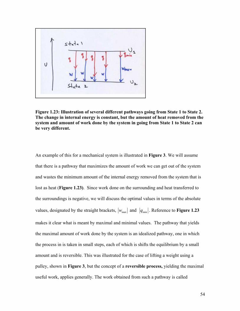
Figure 1.23: Illustration of several different pathways going from State 1 to State 2. The change in internal energy is constant, but the amount of heat removed from the system and amount of work done by the system in going from State 1 to State 2 can be very different.

An example of this for a mechanical system is illustrated in Figure 3. We will assume

that there is a pathway that maximizes the amount of work we can get out of the system

and wastes the minimum amount of the internal energy removed from the system that is

lost as heat (Figure 1.23). Since work done on the surrounding and heat transferred to

the surroundings is negative, we will discuss the optimal values in terms of the absolute

values, designated by the straight brackets, max min and w q . Reference to Figure 1.23

makes it clear what is meant by maximal and minimal values. The pathway that yields

the maximal amount of work done by the system is an idealized pathway, one in which

the process in is taken in small steps, each of which is shifts the equilibrium by a small

amount and is reversible. This was illustrated for the case of lifting a weight using a

pulley, shown in Figure 3, but the concept of a reversible process, yielding the maximal

useful work, applies generally. The work obtained from such a pathway is called

54

reversible work, wrev, and the maximum work that can be done by the system on the

surroundings in going between specified initial and final states is revw . The same

reversible process that maximizes the work ouput must also minimize the amount of

wasted heat (see Figure 1.23). The heat lost to the system in a reversible process is qrev,

and revq is the minimal amount of wasted heat possible for any process going from State

1 to State 2. In the case of the mechanical pulley system in Figure 3, the reversible

process wasted none of the potential energy as heat, but this is not usually the case, as we

will see in what follows.

If the energy of the system is decreased, as in Figure 1.23, then and rev revw q

report the minimal wasted heat and maximum work output possible The work and heat

are both negative since they each decrease the energy of the system. On the other hand, if

the energy of the system increases, then the values of and rev revw q report the minimal

amount of work needed to take the system to the higher internal energy in a reversible

pathway, which is associated with the maximal amount of heat transferred into the system

to accomplish the transition. The reversible process between any two states defines a

special pathway insofar as the values of wrev and qrev are uniquely defined by the initial

and final states of the system. Hence, both wrev and qrev can also be considered to be state

functions because they are defined by the states themselves.

In the 1850�’s, Rudolf Clausius recognized the usefulness of defining a new state

function which he called entropy, S, where

revsys

sys

dqdST

(1.44)

55

Equation (1.44) says that for a small change of state of a system, the entropy change,

sysdS , is defined as the reversible heat required for the transition, dqrev, divided by the

temperature of the system at the instant of the heat transfer,Tsys. Entropy is measured in

�“entropy units�” or e.u., measured in joules per kelvin (JK-1). Since both Tsys and dqrev are

state functions, it follows that dSsys is also a state function, and is absolutely defined by

the initial and final states of the system. It is convenient to consider infinitesimal changes

of state (differential format) so that the temperature (Tsys) can be considered to be

constant.

Since , we can substitute from the definition of entropy in max mindU dw dq

(1.44) to get

max sysdw dU TdS (1.45)

The entropy change of the system is related to that portion of the internal energy which is

unavailable to do work. The product sysTdS has units of energy (joules).

If the initial and final states have different temperatures (T1 and T2), then we can

integrate to find determine the value of sysS . This is the equivalent of adding up the

changes in dSsys for a series of small steps between the two endpoints, as pictured in

Figure 1.8.

2

1

Staterev

syssysState

dqST

(1.46)

Note that the reversible addition of heat to a system at low temperature changes the

entropy by a larger amount than if we add the same amount of heat reversibly to a system

at higher temperature.

56

It also follows from the definition of entropy in (1.44) that in any other pathway

other than the idealized �“reversible�” pathway,

irrevsys

sys

dqdST

(1.47)

where the signs of both dSsys and dqirrev are negative in Figure 1.23 but dSsys is a smaller

negative number.

Of course, all this is just a matter of definitions and is not particularly useful

without some way of relating sysS to measurable properties of the system. It was the

genius of Boltzmann to connect this thermodynamic definition of entropy to the concept

of multiplicity, defined in equation (1.19). Indeed, one can start with Boltzmann�’s

equation (1.19) and mathematically derive the thermodynamic definition of entropy (we

will not do this), though this equivalence is certainly not evident on first observation. The

microscopic definition of entropy readily explains why the reversible addition of heat to a

system at low temperature changes the entropy to a larger extent than the addition of the

same amount of heat added reversibly to the same system at high temperature. The

increase in multiplicity will be relatively small if one adds heat, thus increasing the

internal energy, at high temperatures, because the energy is already dispersed over

molecules at many energy levels (see Figure 1.10, for example). At low temperatures,

fewer energy levels will be occupied at the start, and the addition of heat will have a

proportionately larger effect.

1.18 Entropy and the Second Law of Thermodynamics

The microscopic definition of entropy (Boltzmann�’s equation) and the Principle

of Multiplicity (Section 1.5) state that any spontaneous process in an isolated system will

57

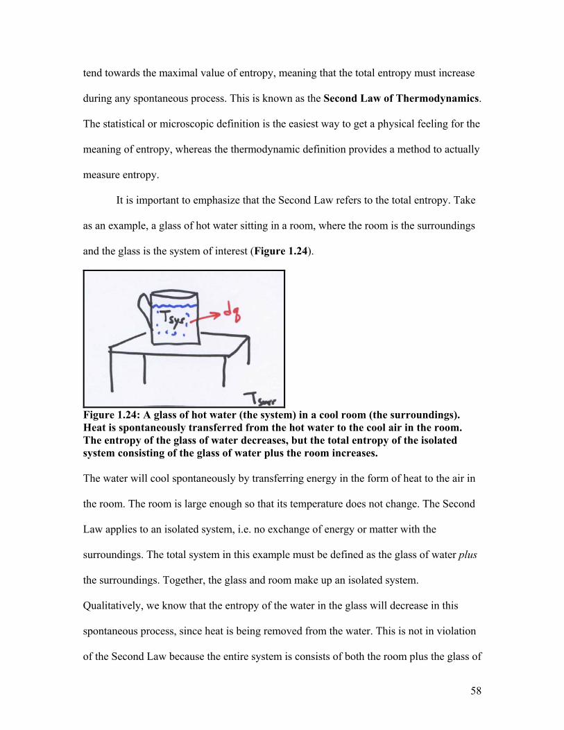
tend towards the maximal value of entropy, meaning that the total entropy must increase

during any spontaneous process. This is known as the Second Law of Thermodynamics.

The statistical or microscopic definition is the easiest way to get a physical feeling for the

meaning of entropy, whereas the thermodynamic definition provides a method to actually

measure entropy.

It is important to emphasize that the Second Law refers to the total entropy. Take

as an example, a glass of hot water sitting in a room, where the room is the surroundings

and the glass is the system of interest (Figure 1.24).

Figure 1.24: A glass of hot water (the system) in a cool room (the surroundings). Heat is spontaneously transferred from the hot water to the cool air in the room. The entropy of the glass of water decreases, but the total entropy of the isolated system consisting of the glass of water plus the room increases. The water will cool spontaneously by transferring energy in the form of heat to the air in

the room. The room is large enough so that its temperature does not change. The Second

Law applies to an isolated system, i.e. no exchange of energy or matter with the

surroundings. The total system in this example must be defined as the glass of water plus

the surroundings. Together, the glass and room make up an isolated system.

Qualitatively, we know that the entropy of the water in the glass will decrease in this

spontaneous process, since heat is being removed from the water. This is not in violation

of the Second Law because the entire system is consists of both the room plus the glass of

58

water. The Second Law states that the total entropy change must be greater than zero for

any spontaneous change in the total system. During the process of the water in the glass

cooling to an equilibrium temperature, the total entropy change will consist of the sum of

the entropy change in the glass of water (which we will refer to as the system) and the

surroundings, i.e., the room. The Second Law states that this total entropy change must

be greater than zero.

0total sys surrS S S (1.48)

In this particular example, there is no work involved, only heat transfer:

for the glass of water; wsys = 0, so Usys = qsys

and for the surroundings; wsurr = 0, so Usurr = qsurr = -qsys

The decrease in the internal energy of the glass of water must be equal to the increase in

the internal energy of the surroundings. Since the internal energy is a state function and

no work is involved, the heat transfer by any pathway will be the same, whether the

pathway is reversible or irreversible. We can now write expressions for the entropy

change.

For the glass of water:

sysrevsys

sys sys

dqdqdST T

2

1

statesys

syssysstate

dqS

T

We need to use the differential expression and then integrate to get the total entropy

change because the temperature of the water is changing as heat is removed, i.e., Tsys is

not a constant.

For the surroundings, where the temperature is constant (Tsurr):

59

2

1

sysrev surrsurr

surr surr surr

statesys sys

surrsurr surrstate

dqdq dqdST T T

dq qS

T T

By our sign convention, heat flowing out of the system is negative, therefore, the entropy

change in the glass of water is negative and the entropy change in the surroundings is

positive.

0

0

0

sys

sys

surr

dqSS

(1.49)

Furthermore, during the entire process, until the very end, the temperature of the water in

the glass is higher than the temperature in the surroundings, sys surr

sys surr

dq dqT T

since sys surrT T , where the brackets dq indicate the absolute value.

Hence, surr sysS S , from which it follows that

(1.50) total sys surrS S S 0

Heat will flow spontaneously from the hot to the cold object, and not in the reverse

direction, since that would result in a decrease in the total entropy of the system and

would violate the Second Law.

The equilibrium position is also defined by the Second Law since heat flow will

cease when the temperature of the water in the glass and in the surroundings are identical.

Note also that the absolute internal energy of the room is much larger than that of the

glass of water. Yet, energy flows from the glass of water to the room. The driving force is

60

to maximize entropy, which corresponds to equalizing the temperatures, and it is not to

equalize the energy content.

Let�’s now look at another example, which will demonstrate the differences

between reversible and irreversible pathways. We start with a gas in a chamber with an

initial pressure of 2 bar, temperature, T and volume of V1. Three pathways are shown in

Figure 1.25 to go to a final state in which the gas has expanded into a volume that is

twice the original volume and at the same temperature. Assuming for simplicity we have

an ideal gas, then we know that the final pressure must be half of the initial pressure,

since and the final volume is double the initial volume. PV nRT

The first pathway shown on the left of Figure 1.25 is to open holes up in the

barrier between the right and left chambers. The gas will re-equilibrate by diffusing into

the full volume. No heat is allowed to exchange with the environment and no work is

done. This is an irreversible process, which is easily imagined if you consider whether it

will go backwards from the final to initial state. This clearly will not happen

spontaneously. Since the temperature is the same in the final and initial states, there is no

change in the internal energy ( U = 0).

61

Figure 1.25: Three processes for expanding a gas from an initial volume in one chamber to double the volume at the same temperature. Process A (left) allows the gas to diffuse from left to right until equilibration. Process B (center) allows the gas to push a piston against no external pressure. Process C (right) is a reversible process where the expanding gas does work and heat transfers from the surroundings to maintain constant temperature. The change in entropy of the system must be the same for all three processes, but only the first two irreversible processes are spontaneous and proceed with a net increase of entropy of the universe (system plus surroundings). The second pathway in the center of Figure 1.25 is also irreversible. In this case,

the gas is allowed to expand, but by pushing the barrier between the chambers to its

limiting position. However, the external pressure, which determines the amount of work

accomplished is zero (Pext = 0), so no work is done. No heat is allowed to exchange with

the chamber, and the final state is identical to that obtained in the first pathway.

The third pathway between the initial and final states is a reversible pathway in

which the gas expansion does work against an external pressure. Furthermore, to

maintain the temperature, we must allow heat to enter the system from the

surroundings.To make this reversible, the external pressure needs to be adjusted

continuously so that it is just slightly less than the internal pressure forcing the piston out.

In this way, each small step is at equilibrium throughout the process. The amount of work

done is determined by integration.

2 2

1 1

2

1

ln ln 2V V

revV V

VdVw PdV RT RT RTV V

(1.51)

where the final volume is twice the initial volume. The final state is exactly the same is in

the two irreversible pathways, and since U = 0 (no change in internal energy)

ln 2rev revq U w RT (1.52)

62

We can use the reversible pathway to determine the change in entropy of the

system, i.e., the gas in the chamber.

ln 2revsys

qS RT

(1.53)

Since entropy is a state function, the change of entropy of the system must be the same

also for the irreversible processes. For the irreversible processes in this example, there is

no change in entropy of the surroundings since there is no interaction between the system

and environment. Hence,

0 for the irreversible processes, and

S ln 2 0 ln 2

0

surr

total sys surr

total

S

S S RT RT

S

This is consistent with the Second Law, since the spontaneous, irreversible

processes occur with a net increase of the entropy. The reversible process, being always

at equilibrium, will not occur spontaneously. In this case, the entropy change of the

surroundings can be easily calculated from the amount of reversible heat removed from

the surroundings, which is just the negative of the amount of heat transferred into the

system.

ln 2revsurr

qST

R (1.54)

For the reversible process, the net change in entropy is zero, taking into account both the

system and the surroundings.

(1.55) ( ln 2 ln 2) 0total sys surrS S S R R

63

1.19 The thermodynamic limit to the efficiency of heat engines, such as the

combustion engine in a car.

The thermodynamic concept of entropy arose from the need to determine the

maximum efficiency of engines which convert heat to work. Both steam engines as well

as the modern gasoline combustion engines are examples of heat engines. It is useful to

see how the simple application sets a limiting efficiency for heat engines, although such

limitations do not apply to biological systems.

Figure 1.26: Schematic of the thermodynamics of a heat engine, such as the combustion engine in a car. Following the combustion of gasoline and oxygen in the piston cylinder, some of the heat from the hot gases (Thot) is converted to useful work and the remainder is lost to the surroundings (Tcold). The requirement that the total entropy must increase limits the efficiency since the only way to increase the total entropy is to transfer heat to the surroundings. In a combustion engine, gasoline and oxygen are combined and a combustion

reaction generates a large amount of heat. Heat is removed from a hot object, in this case

corresponding to the gases inside a piston and converted to work, e.g., rotating the

crankshaft of an automobile engine. Some heat is exhausted to the surroundings.

64

The mechanism of how the work is generated, e.g., expanding gases increasing the

pressure within the piston, is not relevant for this problem. Figure 1.26 is a schematic of

a heat engine from a thermodynamic perspective. Consider one cycle of the engine. We

have a hot object at temperature Thot, the gases in the piston, from which an amount of

heat is removed, and a cold object, the surroundings on which work is done and

which also receives exhaust heat . Since

hotq

coldq hot coldw q q (where since it is

leaving the system), we can define the efficiency of the heat engine as the fraction of the

energy removed from the engine which is converted to work.

0hotdq

1 cold

hot hot

qwq q

(1.56)

The change in entropy of the total system, is the sum of the entropy change in the engine

(hot) and the surroundings (cold). If we assume the exchange of heat does not alter the

temperatures, for simplicity, then

hot coldtotal sys surr

hot cold

q qS S ST T

(1.57)

Let�’s see what happens if all of the energy taken from the engine as heat (qhot) is

converted to work. Then and, consequently, and 0hot coldq w q hottotal

hot

qST

. However,

since (energy is removed from the system), it follows that 0hotq 0totalS . It is

impossible to convert all the heat removed from the engine in the form of work since this

would violate the Second Law of Thermodynamics.

65

In order to convert heat to work, we need to take some of the heat from the hot system

and transfer it to the surroundings. It is the increase in entropy in the �“cold reservoir�” or

surroundings which drives the system forward spontaneously.

The criterion for a spontaneous process is that 0cold hottotal

cold hot

q qST T

, from which we

can conclude that cold cold

hot hot

q Tq T

. Therefore, from equation (1.56)

1 cold

hot

TT

(1.58)

There is a thermodynamic limit to the efficiency for any engine that converts heat to

work, whether it is a steam engine or a gasoline combustion engine, and this limit

depends on the operating temperature of the engine and the temperature of the

surroundings. At a high operating temperature, the efficiency is greater. For a typical

gasoline combustion engine in a car, 380 K and T 300 Khot coldT , giving a limiting

efficiency 0.21hot

wq

. Nearly 80% of the energy is wasted as heat lost to the

environment.

Is this relevant for biological systems? Not really. We don�’t need to worry about

this inefficiency of converting heat to work for biological systems. In principle, there is

no thermodynamic limit to the efficiency of converting one type of work into another.

There will be practical limitations, of course, but generally, biological systems can attain

a high degree of efficiency in interconverting various kinds of work.

The important aspect to note from the examples of the heat engine and the cooling

of a hot glass of water is that the Second Law does not prevent a process in which there is

a spontaneous decrease in entropy in part of a system, as long as the entire process results

66

in a net decrease in entropy. Biological systems are open systems, so any biological

process occurs in contact with the surroundings. What we will do in the next Chapter is

see how we can reformulate the thermodynamic expressions in terms of measurable

properties of the system of interest and not worry about the surroundings, other than to

specify that temperature and pressure.

1.20 The absolute temperature scale.

Up to now we have referred to temperature without defining which scale to use.

The most fundamental scale is the Absolute or Kelvin scale, which conceptually comes

from thermodynamics. The zero point on this scale is the temperature at which the work

done by a system occurs with 100% efficiency and none is wasted. From equation (1.45)

we know that, by this definition, at absolute zero (T = 0)

maxdw dU (1.59)

We can also see this in the expression for the efficiency of a heat engine, equation (1.58).

If the value of Tcold = 0, then the efficiency = 1, and the engine is 100% efficient in

taking heat and converting it to work. This is another definition of the zero point of the

absolute or Kelvin temperature scale.

From a molecular perspective, at absolute zero the entropy content is zero,

meaning that our material is a perfect crystal with only one microscopic state possible

that is consistent with the properties.

(1.60) ln ln(1) 0 at T = 0 KelvinS k W k

We can also see this in the expression for the efficiency of a heat engine, equation (1.58).

If the value of Tcold = 0, then the efficiency = 1, and the engine is 100% efficient in

67

taking heat and converting it to work. This is another definition of the zero point of the

absolute or Kelvin temperature scale.

From a molecular perspective, at absolute zero the entropy content is zero,

meaning that our material is a perfect crystal with only one microscopic state possible

that is consistent with the properties.

(1.61) ln ln(1) 0 at T = 0 KelvinS k W k

Experimentally, absolute zero is at TCelsius = -273.15. The Kelvin scale must be used in all

thermodynamic calculations. The scale is the same as that defined by Celsius, but shifted

so that the zero point is absolute zero. The unit used is defined as the Kelvin (K).

( ) 273.15CelsiusT K T (1.62)

1.21 Summary

We have defined the Principle of Multiplicity, which states that the dispersal of

energy and matter in any isolated system will spontaneously tend towards a state in which

the number of equivalent microscopic states is maximal. This is expressed quantitatively

by the Boltzmann definition of the entropy function. The equilibrium condition for any

isolated system is, thus, that entropy is at its maximum value.

The practical application of the principle of maximizing entropy is provided by

the formal structure of thermodynamics, which shows how entropy can be measured and

quantified by measuring the amount of heat transferred into or out of a system under

specified conditions.

68