Biobjective Scheduling for Joint Parallel Machines with

Research ArticleBiobjective Scheduling for Joint Parallel Machines withSequence-Dependent Setup by Taking Pareto-Based Approach

Wichai Srisuruk ,1 Kanchala Sudtachat ,1 and Paramate Horkaew 2

1School of Manufacturing Engineering, Suranaree University of Technology, Nakhon Ratchasima, Thailand2School of Computer Engineering, Suranaree University of Technology, Nakhon Ratchasima, Thailand

Correspondence should be addressed to Wichai Srisuruk; [email protected]

Received 27 November 2020; Revised 5 August 2021; Accepted 17 August 2021; Published 30 August 2021

Academic Editor: Chen Lin Soo

Copyright © 2021 Wichai Srisuruk et al. This is an open access article distributed under the Creative Commons AttributionLicense, which permits unrestricted use, distribution, and reproduction in any medium, provided the original work isproperly cited.

Modern factories have been moving toward just-in-time manufacturing paradigm. Optimal resource scheduling is thereforeessential to minimize manufacturing cost and product delivery delay. This paper therefore focuses on scheduling multipleunrelated parallel machines, via Pareto approach. With the proposed strategy, additional realistic concerns are addressed.Particularly, contingencies regarding product dependencies as well as machine capacity and its eligibility are also considered.Provided a jobs list, each with a distinct resource work hour capacity, this novel scheduling is aimed at minimizingmanufacturing costs, while maintaining the balance of machine utilization. To this end, different computational intelligencealgorithms, i.e., adaptive nearest neighbour search and modified tabu search, are employed in turn and then benchmarked andvalidated against combinatorial mathematical baseline, on both small and large problem sets. The experiments reported hereinwere made on MATLAB™ software. The resultant manufacturing plans obtained by these algorithms are thoroughly assessedand discussed.

1. Introduction

With the recent advances in modern intelligent manufactur-ing, most industrial works have increasingly been adoptingjust-in-time (JIT) strategy [1, 2]. With this strategy,manufacturing cost and delivery delay are optimized bymeans of meticulous production planning. Among prevailingmachining approaches presently taken by modern factories,unrelated parallel machine (UPM) [3–6] system is investi-gated in this study. In the UPM system, a factory consistsof several machines operating the same task but taking differ-ent time durations. Examples of these factories are lathes andsawmills. Upon commencing any task or restarting an alter-nate one, an operator often has to prepare the machine bymaking appropriate configurations and settings. Theyinclude fitting new moulds, replacing equipped tools, andcleaning contaminated parts. These activities generally incuradditional cost, also known as setting up cost. They areexpressed in terms of spent time (and/or money), whosevalues may be constant or varied as the preceding task. More

specifically, a sequence-independent setup (SIS) [7, 8]remains constant regardless of the previous tasks operatedon the same machine, whereas a sequence-dependent setup(SDS) does not [4, 5, 9, 10]. In addition, while some taskscan well be performed on one machine, they may be prohib-itive on others. For instance, coarse milling may be per-formed on all available machines, while fine milling is onlypossible on specific ones. Another concern faced in typicalindustrial practices is unplanned maintenance (UM) [11]due to faulty resources, especially after a schedule has beenissued.

Provided a list of required productions, i.e., jobs, eachwith associated resource work hour capacity, this paper isaimed at devising an appropriate JIT manufacturing plan.Without loss of generalization ability, UPMs involved in thisstudy were assumed to be of SDS type, where all setups couldbe made equal, otherwise. It took into account productionvariables, typically found in practices, e.g., time and moneyrequired to make an initial machine configuration, givenprecedent tasks, machine standard time, and storage costs

HindawiModelling and Simulation in EngineeringVolume 2021, Article ID 6663375, 19 pageshttps://doi.org/10.1155/2021/6663375

https://orcid.org/0000-0003-0483-6668

https://orcid.org/0000-0001-5025-7961

https://orcid.org/0000-0003-0879-7125

https://creativecommons.org/licenses/by/4.0/

https://creativecommons.org/licenses/by/4.0/

https://doi.org/10.1155/2021/6663375

for products completely in order to meet requested demandeach period (all of which were in integers). The optimalmachine scheduling was determined such that the resultantplan incurred minimum manufacturing cost, while main-taining machine utilization balance. In this study, it was fur-ther assumed that once started, a task could not beoverridden or cancelled, until it was fully completed. To thisend, the state-of-the-art computational intelligence algo-rithms, that is, adaptive nearest neighbour search (ANNS)[12, 13] and modified tabu search (MTS) [14–17], wereemployed and assessed in turns. The resultant schedulingfor small and large problems was subsequently validatedagainst an exhaustive baseline model.

This paper focuses on biobjective unrelated parallelmachine scheduling. Its emphasis is placed on minimizingmanufacturing costs, while maintaining the balance ofmachine utilization, based on Pareto optimality. Its maincontribution is to remedy prohibitively high complexity oftheoretical models by employing heuristic and metaheuristicapproaches, namely, ANNS and MTS. To elucidate its merit,realistic instances of JIT manufacturing environments withpractical conditions were explored in simulations.

The remaining of this paper is organized as follows. Sec-tion 2 reviews the literature and the related works. It pro-vides detailed accounts and critical discussion on machinescheduling problems and state-of-the-art solutions. Section3 describes the proposed scheme by first outlining its keyprocesses, followed by their description and assumptionsmade herein. Section 4 describes the experiments on theabovementioned algorithms, including the characteristicsof data involved and relevant assessments. Subsequently, thissection also demonstrates the merits of the proposed schemeby objectively reporting and discussing the resultant sched-uling, based on designated performance metrics. Finally,Section 5 makes the concluding remarks on the contributionof this study and its prospects.

2. Literature Review

This section focuses on recent research on conditional andconstrained scheduling. In order to devise an optimalmanufacturing plan that minimizes its overall costs, includ-ing those incurred by configuring the machines during theproduction process and by inventory storage, variousapproaches have been taken in the literature. They can becategorized into those based on solving for an exact solutionof some mathematical model and on approximating one bycomputational intelligent techniques. The following subsec-tions start from background on scheduling theory. Afterthat, the definitions of parallel machine scheduling and itsmathematical model are described. On solving such a model,various optimization strategies, both with single and multi-ple objectives, are subsequently reviewed. Finally, the recentand closely related research works to the proposed schemeare discussed.

2.1. Background on Scheduling. Scheduling is one of themanagement schemes that attempts to allocate limitedresources for completing a mission within given timeframe,

possibly under some constraints [18]. In an industrial con-text, a preferable solution to this problem is determined byoptimizing resources’ utilization (i.e., manpower andmachines) with respect to predefined objectives [6, 19, 20].This paper proposed a novel solution to a scheduling prob-lem of a manufacturing system, which was characterized asfollows.

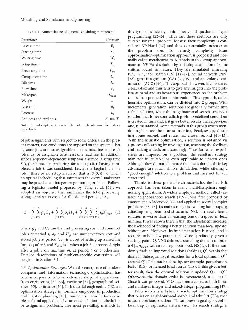
The system consists of a set of n jobs and m machines,denoted by I = fi ∣ i ∈ ½1, n�g, J = fj ∣ j ∈ ½1, n�g, and M = fm ∣ m ∈ ½1,MC�g, where i and j are the indices of job andm is the indices of machine, respectively. The notations ofkey parameters involved in the analyses are listed in Table 1.

Scheduling strategies can be divided into flow shop andjob shop scheduling [21]. The former consists of consecutivemachines or job stations, and each performs different oper-ations. All the jobs are processed by each machine in anexact same sequence, called flow, whereas in the latter group,scheduling is made for each job, whose flow consists of aunique sequence of operations. On solving a schedulingproblem, there exist three techniques normally adopted.First, a mathematical model can be used to find an optimalscheduling by means of, for instance, integer, mixed integer,or dynamic programming [22–24]. Objectives typically con-sidered in the optimization are flow time, makespan, late-ness, number of tardy jobs, tardiness, etc. [25–27]. As theproblem size increases, however, they suffer from excessivecomplexity. Second, dispatching rules or heuristic tech-niques are especially designed to reduce complexity whileoffering acceptable results within reasonable time. Given aset of jobs, these techniques imposed one or more criteria,e.g., first come first served (FCFS), shortest processing time(SPT), longest processing time (LPT), and earliest due date(EDD) [25, 28]. Techniques in this group also consider sim-ilar objectives that do those in the former one. Third, neigh-bourhood search finds an optimal solution more efficiently,especially for larger problems, by incrementally updatingthe current best solution, taking into account informationfrom its neighbours. They include tabu search, simulatedannealing, and genetic algorithms [14, 29, 30].

Furthermore, scheduling also differs by machine layouts.Single machine scheduling is trivial and usually adopted indecomposition of a more complex manufacturing. On theother hand, for the parallel machines, single-process jobsare released to a pool of machines working in parallel. Thescheduling problem is now reduced to making two decisions,i.e., job allocation and its sequence. This type of schedulingcan be further divided by the functions of associatedmachines, which are identical (IPM), nonidentical (NPM),and unrelated parallel machine (UPM) [3–6]. This researchfocuses on UPM, where each machine can process a givenjob at a different speed. Since a machine can process differ-ent jobs, when starting a new one, a setting up is usuallyneeded [7–10]. Therefore, time and cost used in this opera-tion depend on involved jobs and their sequence.

2.2. Mathematical Models of Parallel Machine Scheduling.Provided a problem of scheduling a set of n jobs (I and J)onto m parallel machines (M), as described in Section 2.1,a mathematical model attempts to plan an optimal sequence

2 Modelling and Simulation in Engineering

of job assignments with respect to some criteria. In the pres-ent context, two conditions are imposed on the system. Thatis, some jobs are not assignable to some machines and eachjob must be assignable to at least one machine. In addition,since a sequence-dependent setup was assumed, a setup timeS ði, jÞ ≥ 0, used in preparing for a job j after having com-pleted a job i, was considered. Let, at the beginning for ajob i, there be no setup involved, that is, S ð0, iÞ = 0. Then,an optimal scheduling that minimizes the overall makespanmay be posed as an integer programming problem. Follow-ing a logistics model proposed by Tong et al. [31], weadopted an objective that minimizes the total processing,storage, and setup costs for all jobs and periods, i.e.,

Z = 〠n

j=1〠T

t=1gjtCjt + 〠

n

j=1〠T

t=1ojtHjt + 〠

n

i=1〠n

j=1〠M

m=1〠T

t=1sijXijmt , ð1Þ

where gjt and Cjt are the unit processing cost and counts ofjob j at period t, ojt and Hjt are unit inventory cost andstored job j at period t, sij is a cost of setting up a machinefor job j after i, and Xijmt is 1 when a job j is processed rightafter a job i on machine m, at period t or 0 otherwise.Detailed descriptions of problem-specific constraints willbe given in Section 3.1.

2.3. Optimization Strategies. With the emergence of moderncomputer and information technology, optimization hasbeen incorporated into an extensive range of applications,from engineering [32, 33], medicine [34], geographical sci-ence [35], to finance [36]. In industrial engineering (IE), anoptimization strategy is normally employed in productionand logistics planning [18]. Enumerative search, for exam-ple, is found applied to solve an exact solution to schedulingor assignment problems. The most prevailing methods in

this group include dynamic, linear, and quadratic integerprogramming [22–24]. Thus far, these methods are onlysuitable for small problem, because their complexity is con-sidered NP-Hard [37] and thus exponentially increases asthe problem size. To remedy complexity issue,approximation-optimization approach is proposed and nor-mally called metaheuristics. Methods in this group approxi-mate an NP-Hard solution by imitating adaptation of someentities found in nature. They are simulated annealing(SA) [29], tabu search (TS) [14–17], neural network (NN)[38], genetic algorithm (GA) [31, 39], and ant-colony opti-mization (ACO) [40]. This approach, however, is considereda black-box and thus fails to give any insights into the prob-lem at hand and its behaviour. Experiences on the problemcan be incorporated into optimization. This approach, calledheuristic optimization, can be divided into 2 groups. Withincremental generation, solutions are gradually formed intoa final solution, while the neighbourhood search strategy asolution that is not contradicting with predefined conditionsis created in turn and, if it gives better results than a previousone, is maintained. Some methods in this group worth men-tioning here are the nearest insertion, Petal, sweep, clusterfirst route second, and route first cluster second [41–43].With the heuristic optimization, a solution is obtained viaa process of learning by investigation, assessing the feedbackand making a decision accordingly. Thus far, when experi-ences are imposed on a problem, the resultant strategymay not be suitable or even applicable to unseen ones.Although they do not guarantee the best solution, their keyadvantages are much simple simulation, while offering a“good enough” solution to a problem that may not be wellstructured.

Thanks to those preferable characteristics, the heuristicapproach has been taken in many multidisciplinary engi-neering applications. A widely employed method, called var-iable neighbourhood search (VNS), was first proposed byHansen and Mladenović [44] and applied to several complexproblems [45, 46]. Its main strategy is avoiding local traps byadjusting neighbourhood structures (NS), if a newly foundsolution is worse than an existing one or trapped in localminima. It was shown therein that the adjustment increasesthe likelihood of finding a better solution than local updateswithout one. Moreover, its implementation is trivial, and itrequires only a few parameters. More specifically, given astarting point, Q, VNS defines a searching domain of ordern ∈ ½1, nmax�, within its neighbourhood, NS ðQÞ. It then ran-domly finds an improved solution (shaking), Q′, within thatdomain. Subsequently, it searches for a local optimum Q′′,around Q′. This can be done by, for example, perturbation,basic (BLS), or iterated local search (ILS). If this gives a bet-ter result, then the optimal solution is updated Q⟵Q′′.Otherwise, the domain order is incremented, n⟵ n + 1.Since it was proposed, VNS has been applied to both linearand nonlinear integer and mixed-integer programming [47].

Tabu search is a hybrid discrete optimization strategythat relies on neighbourhood search and tabu list (TL), usedto store previous solutions. TL can prevent getting locked inlocal trap by aspiration criteria (AC). Its search strategy is

Table 1: Nomenclature of generic scheduling parameters.

Parameter Notation

Release time Ri

Starting time StiWaiting time Wi

Setup time Sij

Processing time Pim

Completion time Ci

Idle time Im

Flow time Fi

Makespan Cmax

Weight wi

Due date di

Lateness Li

Earliness and tardiness Ei and Ti

Note: the subscripts i, j denote job and m denote machine indices,respectively.

3Modelling and Simulation in Engineering

deterministic and specified by recency and frequency condi-tions. In addition, the performance can be enhanced by twomechanisms, i.e., intensification and diversification. Pro-vided a search space and radius (R), counter, a TL, and ter-mination criteria (TC), tabu search algorithm starts byrandomly picking an initial solution, S0 within the searchspace. It then randomly gathers N neighbours within radiusR around S0 and stores in a set S1 ðRÞ. An objective functionis evaluated in turn for each point in this set, and the onethat gave the best (minimum cost) solution is marked as S1. If S1 ≤ S0, the previous solution, S0 is stored in the TLand the solution is updated, S0⟵ S1. Otherwise, S1 isstored in the TL. The process is repeated until TC are met,and the optimal solution is the current S0. Basic TS is ratherslow and can get trapped in local minima. Adaptive tabusearch (ATS) that incorporates backtracking and adaptiveradius mechanisms was proposed to elevate the issues [48].With ATS, after a new solution is updated, backtracking isinvoked when it is locked by local solution. Search radiusis also adapted as it reaches convergence.

On solving biobjective scheduling problems, this paperused both heuristic and metaheuristic methods, respectively,called adaptive nearest neighbour search (ANNS) and mod-ified tabu search (MTS). Pareto optimality of the final pro-duction plans and their performance metrics were thenvalidated against enumerative search.

2.4. Single- versus Multiobjective Optimization. Single-objec-tive optimization is aimed at finding the best solution to aproblem, under specified constraints. Generally, it consistsof three components, i.e., vector of decision variables, con-straints, and an objective function. Unlike its single counter-part, multiobjective optimization finds, within feasibleregions, the best solutions with respect to more than oneobjective functions, whose values may be maximized and/orminimized. As described in Section 2.1, a scheduling is anNP-Hard problem, whose best solution is not always feasiblewith a typical algorithm. Much research in this area thusopts for its approximation set instead. This approximationusually involves 2 processes [49, 50], i.e., fitness assignmentand population diversification. This is to ensure that theapproximated solution is close to the exact one and is uni-formly distributed, from one end of the domains to another.Several approaches were taken to assign a fitness, e.g., goalprogramming, vector evaluation, Goldberg or nondomi-nated sorting, Fonseca and Fleming sorting, and accumulateranking density strategy (AARS) [51–53].

In the proposed biobjective strategy, for instance, ourprimary objective function was to minimize all costsincurred by production. To ensure the proper distributionof decision variables, a secondary objective that aims at bal-ancing machine utilization was incorporated.

2.5. Related Works. Scheduling on parallel machines hasattracted much interest in the past decades. A range of strat-egist and objectives have been proposed in the literature.Ruiz-Torres et al. [54], for instance, scheduled different par-allel unrelated resources, aiming at reducing the number oflate jobs. In that work, both machines with different process

times and varying numbers of line staffs were allocated at agiven period. They divided the problems into two scenarios,which were parallel machine flexible resource scheduling(PMFRS) and unspecified parallel machine flexible resourceone (UMFRS). The problems were solved by a computerprogram. On scheduling unrelated parallel machines, Kimet al. [55] employed different objectives, taking into accountboth setup time and total weighted tardiness. They took aheuristic approach with two objectives, which were earliestweighted due date (EWDD) and shortest weighted process-ing time (SWPT), and two optimizers, namely, two-levelbatch scheduling (TLBS) and simulated annealing (SA). Edisand Oguz [56] studied unrelated parallel flexible machinesand proposed two mathematical models, called PMFRSand UPMFRS, but aiming at minimizing the completiontime. Much recently, focus has been moving onto optimiza-tion strategies. Polyakovskiy and Hallah [57] studied multi-stage scheduling by considering earliest weighted late jobsof parallel machines. It was observed that each job requireda different process time and was to be delivered at a differentdue date. Therein, the mixed integer programming (MIP)method, called MASH, was employed to solve the bottleneckproblem in multistage scheduling. A just-in-time (JIT)scheduling approach was taken by Kayvanfar et al. [1, 58]to minimize total tardiness and the number of early com-pleted jobs. The overall cost thus depended on whether jobswere completed earlier or later than specified due dates. Sim-ilarly, an MIP method was employed. It was assumed thatthere was no job insertion and the unrelated parallelmachines had different processing rates. Nonetheless, theirmethod suffered from the problem size and, without hybridintegration, is suitable for only small ones. With similarmachine condition, Zhang et al. [59] minimized weightedaverage tardiness by means of reinforcement learning (RL).In their experiments, release time and due date were ran-domly specified, and the resulted scheduling was found tooutperform all the methods being benchmarked.

In addition, there have been a number of most recentstudies, focusing on parallel machines, JIT approaches, mul-tiobjective strategies, and the combinations of these areas,and hence worth explored here. Majority of early worksassumed single objective strategy [60–65]. In 2014, Kayvan-far and Teymourian [60] proposed an intelligent water drop(IWD) algorithm to schedule unrelated parallel machines. Itwas validated on five machines, with small and large num-bers of jobs. However, it did not consider setup time. Thiswork was later extended to account for not only identical[61] but also unidentical [63] machines. The former stillfollowed previous optimization strategy, whereas the latterproposed a parallel net benefit compression–net benefitexpansion (PNBC-NBE) algorithm. These methods differedfrom their precedence in that the former considered JITmanufacturing with controllable process time, while the lat-ter focused on sequence-related setup times. Another similarwork was proposed by Lin and Ying [62]. They focused on anew optimization algorithm, called hybrid artificial bee col-ony (HABC), which was compared against TS, natureinspired, and RSA optimizations. It was validated on biggerproblems. Since then, a number of works explored various


metaheuristic optimization strategies [64, 65] on similarproblems. Thus far, these methods did not consider cycletime. Biobjective scheduling for batch processing with nosetup time was considered in subsequent attempts [66, 67].Similar to the previous works, they also used metaheuristicoptimization. Taking into account sequence-dependentsetup time, Yepes-Borrero et al. [68] proposed minimizingboth makespan and number of resources, by using greedyalgorithm. On solving multiobjective scheduling problems,Kayvanfar et al. [69, 70] used SA and GA as optimizers,for unrelated and identical parallel machines, respectively.Neither setup time nor cycle time was considered in thoseworks, but the latter considered JIT approach. At least oneor more limitations are shared by the abovementionedworks and different from ours. They include the omissionsof sequence-dependent setup time, process time, and cycletime, as well as smaller numbers of objectives.

3. Proposed Method

This paper focuses on scheduling and its analyses on unre-lated parallel machines, whose setup times were sequencedependent. Furthermore, it was assumed that assigning ajob to any machine is subject to its predefined eligibilityand that deliveries were made at production intervals. Thistotal cost minimization problem was solved by using bothmathematical model and computational intelligence methods.Later, Pareto strategy [71] for biobjective problem was consid-ered, by integrating balanced machine utilization into the costfunctions. Likewise, the scheduling results obtained by theproposed computational intelligence methods were comparedagainst those by the mathematical model baseline.

3.1. Mathematical Model for Scheduling Problems. This sec-tion describes a mathematical model referred to as a baselinein benchmarking. With this model, it was assumed that (1)machines were unrelated and parallel, (2) their setup timesdepended on production sequence, and (3) their eligibilityfor given jobs was prespecified. The objective of their sched-uling was to minimize the makespan by using an integerprogramming method.

The input variables were scheduling or assignment table(X) and quantity units of processed jobs (N) at each period.Given these variables, completed (C) and quantity inventoryunits stored at the end of period (H) would be then deter-mined. Finally, the cost function (Z) would be evaluated,given system parameters, from the numbers of assigned,produced, and stored jobs, as expressed in Equation (1). Spe-cifically, the system parameters were (sequence dependent)setup times (S), unit production (G), and storage (O) costs,respectively.

To ensure realistic scheduling, there are some con-straints worth considered and described as follows.

In each production round, the quantity units of proc-essed job j must meet delivery demand, while the total pro-duction time must fall within specified working hours, asexpressed in

Cjt ≤WorkHour, ∀j,t: ð2Þ

In addition, the quantity units of processed job j pro-duced on those machines in total (all periods, t) must be apositive integer and was no less than the lower lot size.Finally, a job assigned to a machine must be within its capac-ity. These constraints are given in Equations (3) and (4),respectively.

〠MC

m=1Njmt ≥ LowerLotSize, ∀j,t j ≠ 1, ð3Þ

Njmt ≤ BigM · Zjmt , ∀j,m,t j ≠ 1: ð4ÞWith this scenario, provided the problem parameters,

i.e., jobs, working period and hours, and machines, as wellas resources’ data, i.e., production and release time, demand,machine eligibility, production and storage unit costs, andsetup cost, scheduling gives an optimal binary productiontable (Xijmt), as well as corresponding quantity units of eachprocessed job on each machine (Njm) total complete time(Cj), at each period. To maintain valid production table, allelements were asserted by auxiliary variables (Ajmt , Bjmt) asdefined in Equations (5) and (6). This ensures, for instance,that a machine must be assigned with at least one job, asgiven in Equation (7).

〠n

i=1,i≠jXijmt = 1 − Ajmt , ∀j,m,t j ≠ 1, ð5Þ

Bjmt + Ajmt = 1, ∀j,m,t j ≠ 1, ð6Þ

〠MC

m=1Ajmt = 1, ∀j,t j ≠ 1: ð7Þ

During the integer programming, plausible schedulingwas subject to specific constraints, as follows. The quantityunits of stored job j at period t, Hjt , were equal to the job jpreviously stored (Hjt−1) and currently processed on allmachines but subtracted by the amount required. That is,

Hjt = 〠M

m=1Njmt − djt , ∀j,t t = 1, ð8Þ

Hjt =Hj,t−1 + 〠M

m=1Njmt − djt , ∀j,t t ≠ 1: ð9Þ

Provided that a machine was able to process both jobs iand j and that job j was processed right after job i, then thetime that job j (Cjt) was completed was equal to the timewhen a previous job (Cit) was completed, plus sequencedependent setup time (Sij) and time used to process the spe-cific amount of that job (Pjm ·Njmt). The resulted completetime (Cjt) must be within working hours of that period. Fur-thermore, when subtracted by setup and process time, itshould be later than its release time (Rj). That is, ∀i,j,m,tand i ≠ j, j ≠ 1,


Cjt − Cit + BigM · 1 − Xijmt · Eim · Ejm

� ��

≥ PjN jmt + Sij · Xijmt · Eim · Ejm

� �,

ð10Þ

Cjt − Pj ·Njmt − Sij · Xijmt · Eim · Ejm

� �� ≥ Rj: ð11Þ

Regarding a job sequence, only one job j could succeedanother job i, and it should be processed by only onemachine, and vice versa. In other words, at a given period,a job might not be distributed to different machines. Fur-thermore, preceding and succeeding jobs must be different,or a job could not be processed if it had just been completedon that machine. These constraints are realized by Equations(12)–(15), respectively.

〠n

i=1〠M

m=1Xijmt · Eim · Ejm = 1, ∀j,t j > 2, ð12Þ

〠n

j=1〠M

m=1Xijmt · Eim · Ejm = 1, ∀i,t i > 2, ð13Þ

〠n

i=1Xijmt − 〠

n

w=1Xjwmt = 0, ∀i,j,m,t i ≠ j, j ≠w, ð14Þ

Xjjmt = 0, ∀j,m,t: ð15ÞTo ensure utilization constraints, a machine should have

at least one first job and one last, maybe different, job, asexpressed in Equations (16) and (17), respectively. Likewise,a job should be assigned first and last, each time to at leastone, maybe different, machine, as expressed in Equations(18) and (19), respectively. Lastly, any given job must beassigned to only one machine, as expressed in Equation (20).

〠n

j=2X1jmt · Ejm = 1, ∀m,t , ð16Þ

〠n

i=2Xi1mt · Eim = 1, ∀m,t , ð17Þ

〠n

j=1〠MC

m=1X1jmt · Ejm =MC, ∀t j ≠ 1, ð18Þ

〠n

i=1〠MC

m=1Xi1mt · Eim =MC, ∀t i ≠ 1, ð19Þ

〠M

m=1Xijmt + Xjimt

� �· Eim · Ejm ≤ 1, ∀i,j,t i ≠ j: ð20Þ

To maintain integer computability, values in schedulingtables were only binary, i.e., 1 or 0, depending on whetherany assignment of a job after completion of another onewas eligible for that machine at that period or otherwise,respectively. Finally, numbers of processed and stored jobsand that of process time per job must be positive integers.Since these constraints are self-explanative, their detailedexpressions are hence omitted.

The outputs of scheduling process were, for a given job iand at period t, (1) number of stored job (Hit), (2) quantityunits of processed jobs at a machine m (Nimt), and (3) timespent on processing the job (Cit).

3.2. Computational Intelligence Methods. This sectiondescribes the proposed heuristic and metaheuristic methodsfor solving unrelated parallel scheduling problem. Herein,we employed adaptive nearest neighbour search (ANNS)and modified tabu search (MTS). Their processes and for-mulations in the present context are provided in the follow-ing subsections.

3.2.1. Adaptive Nearest Neighbour Search (ANNS). TheANNS starts by specifying an initial solution and a best solu-tion table. Upon entering the updating loop, neighbouringsolutions with respect to job sequence (S) and processingdemand (D) were created, adaptively. More specifically, theneighbours were defined by offsetting a current solution bydistances of a 20–22, multiplied by adaptive step size, i.e.,

S isð Þ = −4,−2,−1, 0, 1, 2, 4f g ×Ws × is, ð21Þ

D idð Þ = −4,−2,−1, 0, 1, 2, 4f g ×Wd × id , ð22Þwhere is and id were the indices to job sequence pair andprocessing demand tables, respectively, whose memberswere prepopulated by all possible combinations of therespective variables. Specifically, for a problem with fourjobs, there were 4! = 24 possible sequences. The processingdemand was computed for each period and product fromits actual demand subtracted by that already processed andstored in an inventory. The values were lower bounded byeconomic order quantities (EOQ) and lower lot size. In addi-tion, S and D were created neighbours andWs andWd wereadaptive steps, of the job sequence and the processingdemand indices, respectively.

Subsequently, objective functions were evaluated, giveneach neighbour in turns, and the best solution would beappended to the best solution table. At each iteration, solu-tions in this table would be sorted by their objective func-tions. If the size of this table was greater than a predefinedvalue, the worst solutions so far would then be discarded.Later, the remaining ones were assessed, and if there wereexcessive numbers of duplicated solutions, then the adaptivesteps (Ws,d) were adjusted. The best solution would be cho-sen in the next iteration. This ANNS process was iterateduntil convergence or the number of rounds reached a speci-fied limit.

3.2.2. Modified Tabu Search (MTS). Similarly, MTS alsostarted by specifying an initial solution and a best solutiontable, but it also created a tabu table. Adaptive table indexingof neighbours was evaluated following that of ANNS. Evalu-ation of objective functions and updating of the best solutiontable were also the same as before. However, once the bestsolution table had been updated, the tabu list was modified.If the best solution in the current round was no better thanthe previous ones, it would be added to the tabu list. Thiswould effectively enable backtracking solutions to existing


tabu members, should it be locked in local minima. Likewise,this process was iterated until convergence or the number ofrounds reached a specified limit.

The diagram of ANNS and MTS processes is illustratedin Figure 1.

3.3. Pareto-Based Approach toward Biobjective Scheduling. Itwill be later demonstrated that, with single objective func-tion, although production cost (Z), expressed in Equation(1), was optimized, the machine utilization was not. Themachine utilization was defined as a ratio between its oper-ational and total working hours. Therefore, in the presentcontext, another objective was to maximize the minimummakespans (U), normalized over all involving machines,that is,

U = min1≤j≤n

∑Tt=1Cjt

∑nj=1∑

Tt=1Cjt

: ð23Þ

To balance between production cost and resource utili-zation, the main contributions of this paper are to devise abiobjective model of an unrelated parallel machine schedul-ing problem and then to obtain their Pareto solutions. Con-sider a 2-objective minimization problem:

min F Xð Þ F Xð Þ = Z Xð Þ,U Xð Þf g: ð24Þ

A solution X is said to dominate a solution Y if Z ðXÞ≤ Z ðYÞ and U ðXÞ ≤U ðYÞ, and there is at least one of thesefunctions, where X yields strictly lower value than does Y .Solution X is called Pareto optimal if it is not dominatedby any other feasible solutions. To this end, three Paretostrategies are proposed.

(a) Pseudo-Pareto Optimal. A set of some optimal pro-duction plans with respect to the primary objective,i.e., production cost, was collected. Among theseplans, the one with optimal utilization was selected.

(b) Parallel Pareto Optimal. Both primary and machineutilization objective functions were evaluated, and aset of optimal scheduling with respect to each ofthese objectives was collected, separately. Upon con-vergence, the optimal one from both groups wasselected.

(c) Serial Pareto Optimal. The production objectivefunction was first evaluated, but an optimal onewould be admissible in the candidate list, only if itsutilization was also within an acceptable range.Again, upon convergence, the optimal one wasfinally selected.

3.4. Experiments. Herein, three types of scheduling prob-lems, which were reference, and those with small and largesizes, were considered. For each problem, the input parame-ters were number of jobs (nJob), number of periods (nPeriod), number of machines (nMachine), working hours(WorkHour), and order or lot size (LotSize). The conditionalparameters were production and release time, demand,machine eligibility, and the unit costs for production, stor-age, and sequence-dependent setup. Following recommen-dations made by Afzalirad and Rezaeian [72], theparameters were specified as listed in Table 2.

For each problem, their overall cost and schedulingtimes were compared, among integer programming of themathematical model (3.1), ANNS (3.2.1), and MTS (3.2.2).

To obtain the results reported as follows, the mathemat-ical models were solved by LINGO 11.0 software, while theANNS and MTS were implemented on MATLAB™. Bothprograms were run on a personal computer (PC), installed

Initial solutionsbest solutions table

Adaptive neighborsets : S and D

Evaluate objectivefunction

Append to the best solution table

Sort and remove

Update tabu list

Termination?NO

End

YES

Begin

Termination criteria• Convergence• Maximum number of rounds• Excessive duplicate solutions

Tabu list

Figure 1: Diagram of ANNS and MTS methods. Light boxes with solid lines and dark boxes with dotted lines indicate common steps andthose required only by MTS, respectively.


with Windows 10 64-bit operating system. The PC wasequipped with an Intel I5–6200U processor, clocked at2.30GHz and 4GB main memory.

4. Results and Discussion

This section reports experiment results and relevant discus-sion on three scheduling methods, namely, the mathematicalmodel, ANNS, and MTS. They were evaluated by reference,small, and large problems.

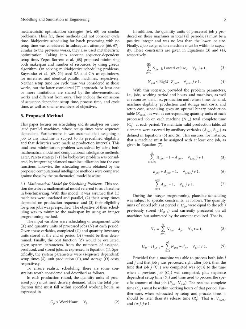
4.1. Reference Problems. As preliminary model assessments,a set of reference problems was first solved using the math-ematical model. Specifically, scheduling 6 and 9 jobs (J),on 2 machines (M), and within 3 and 6 periods (P) wereassessed. Their objective functions as expressed in Equation(1) and corresponding computing time are listed in Table 3.Note that, with 09J02M06P case, processing steps and timetaken were extremely long and consumed excessiveresources on our system. Its details were hence not includedin the table (case 4∗). The values in objectives column areglobal optimum found in each case.

It is evident from Table 3 that as the problems gotslightly more complex, for instance, from 6 to 9 jobs, thesolver steps and hence scheduling time exponentiallyincreased. In fact, with our setting, the integer programmingprocess took about 4 days already to complete. This methodis therefore not suitable for larger scheduling problems, andalternatives would be required, especially for actual JITmanufacturing.

Figure 2 depicts an example of scheduling for the09J02M03P, while Figure 3 provides, at each period, thenumber of jobs being ordered (demanded) and stored inthe inventory and those being processed on each of thetwo machines. Note from both figures that only eight realjobs appear. This is due to the first job being exploited as adummy to satisfy the first and last job constraints, asdescribed in Section 3.1.

In the subsequent experiments, ANNS and MTS werebenchmarked against the mathematical model on the sameproblems. However, because both ANNS and MTS involved

uniformly random initializations, they were each executedfor six runs. The objective functions and scheduling timefor all those runs and the respective averages as well as thedifferences than those obtained by the mathematical modelare listed in Table 4.

Evidently, with small problems (06J02M03P), ANNSand MTS took similar processing time to integer program-ming on the mathematical model. Even when these prob-lems getting much complicated and hence themathematical model failed to schedule within reasonableamount of time, computing time required by ANNS andMTS remained roughly unchanged, while giving similarobjective values to the mathematical model. Furthermore,closer inspection on the deviations of their objective valuesfrom those obtained by the mathematical model was per-formed. The results are plotted in Figure 4. It is observedthat ANNS results were much consistent and closer to thebaseline in cases of fewer jobs. The opposite is true, however,for bigger problems.

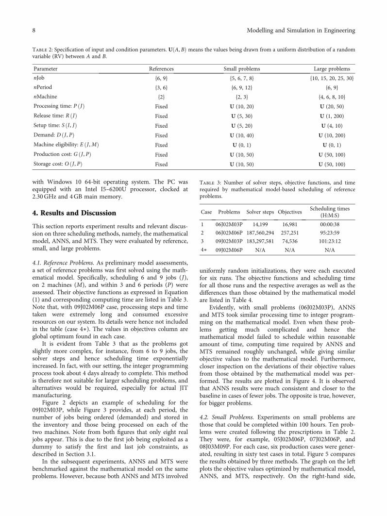
4.2. Small Problems. Experiments on small problems arethose that could be completed within 100 hours. Ten prob-lems were created following the prescriptions in Table 2.They were, for example, 05J02M06P, 07J02M06P, and08J03M09P. For each case, six production cases were gener-ated, resulting in sixty test cases in total. Figure 5 comparesthe results obtained by three methods. The graph on the leftplots the objective values optimized by mathematical model,ANNS, and MTS, respectively. On the right-hand side,

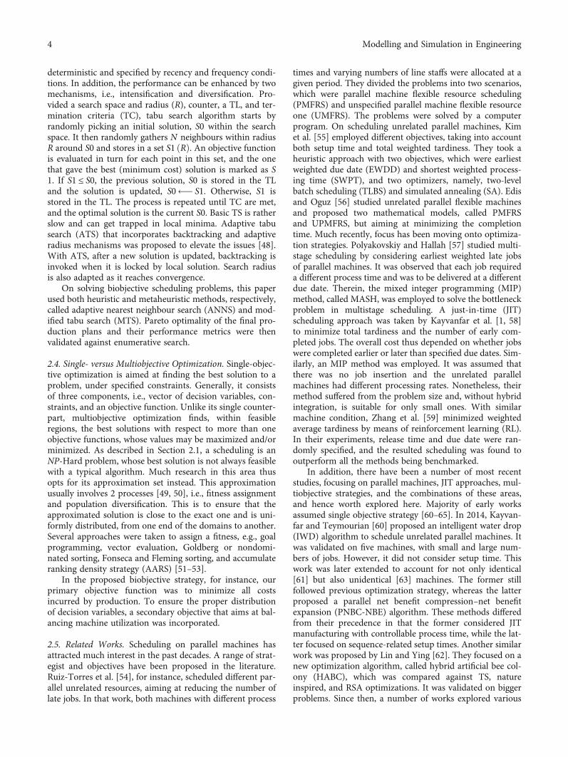
Table 2: Specification of input and condition parameters. UðA, BÞ means the values being drawn from a uniform distribution of a randomvariable (RV) between A and B.

Parameter References Small problems Large problems

nJob {6, 9} {5, 6, 7, 8} {10, 15, 20, 25, 30}

nPeriod {3, 6} {6, 9, 12} {6, 9}

nMachine {2} {2, 3} {4, 6, 8, 10}

Processing time: P Jð Þ Fixed U (10, 20) U (20, 50)

Release time: R Jð Þ Fixed U (5, 30) U (1, 200)

Setup time: S I, Jð Þ Fixed U (5, 20) U (4, 10)

Demand: D J , Pð Þ Fixed U (10, 40) U (10, 200)

Machine eligibility: E J ,Mð Þ Fixed U (0, 1) U (0, 1)

Production cost: G J , Pð Þ Fixed U (10, 50) U (50, 100)

Storage cost: O J , Pð Þ Fixed U (10, 50) U (50, 100)

Table 3: Number of solver steps, objective functions, and timerequired by mathematical model-based scheduling of referenceproblems.

Case Problems Solver steps ObjectivesScheduling times

(H:M:S)

1 06J02M03P 14,199 16,981 00:00:38

2 06J02M06P 187,560,294 257,251 95:23:59

3 09J02M03P 183,297,581 74,536 101:23:12

4∗ 09J02M06P N/A N/A N/A


percentage differences, compared to the mathematical modelbaselines, are shown. It can be concluded from both graphsthat, for small problems, both ANNS and MTS methodsyielded similar objective values to those by integer program-ming on mathematical model, with differences bounded by 8and 10%, respectively.

4.3. Large Problems. Based on the same criterion, large prob-lems were those that required more than 100 hours to sched-ule. In particular, according to Table 2, they were those with10–30 jobs, to be scheduled on 4–10 machines, within 6–9periods. In total, they would consist of 40 problems, but 15ones, for instance, 10J04M06P, 15J06M09P, 25J08M06P,

Periode-2

Machine-1

Machine-2

0 100 200 300 400 500 600 700 800 900 1000

Machine-1

Periode-1

Periode-2

Machine-2

Machine-1

Machine-2

2

0

0

2

5

2

0 3035 45 58 73 85 110

10 31 66 76 96 122 330

15 28 55 80 85

8 13 53 77 217 246

295

666

100 200 300 400 500 600 700 800 900 1000

0 100 200 300 400 500 600 700 800 900

Obj.funtion = 74536

1000

60 65 145 158

28 49 259 269

323 335 535

429 455 1007

Figure 2: Scheduling plans for the 09J02M03P case. Each bar represents each of the different jobs.

Periode-1 Periode-2 Periode-3 Periode-4

D1 10

0

0

0

0

0

0

0

10

30

30

40

40

40

40

69

20

55

40

20

10

26

20

16

10

30 35

35

350

10

20

20

35

35

30

3429

60

25

40

25

22

10

2 10

0

00

0

00000000

0

0

0

030

30

20

20

20

20

20

20

20

20

30

30

30

4 30

25

15

15

15

15

25

D2

D3

D4

D5

D6

D7

D8

0 20 40 60 0 20 40 60 0 20 40 60 0 20 40 60

D1

D2

D3

D4

D5

D6

D7

D8

D1

D2

D3

D4

D5

D6

D7

D8

D1

D2

D3

Obj.function = 74536

D4

D5

D6

D7

D8

DemandInventory

Machine-1Machine-2

Figure 3: Periodical jobs that were ordered and stored in inventory and those being processed on each of the two machines.


Table 4: Comparison of objective value and scheduling time between mathematical model, ANNS, and MTS methods on the referenceproblems, i.e., 06J02M03P, 06J02M06P, and 09J02M03P.

CaseRun Objective values Scheduling time (H:M:S), S

Math ANNS MTS Math ANNS MTS

06J02M03P

1

16,981

17,770 18,006

00:00:38

33.5 33.5

2 17,562 17,541 30.5 34.2

3 18,634 17,918 29.5 32.3

4 17,074 17,918 34.5 31.9

5 17,234 17,986 33.5 32.0

6 17,394 18,006 36.5 32.0

AVG 17,611 17,896 33.0 32.7

Δ 630 (3.71%) 915 (5.39%)

06J02M06P

1

257,251

262,467 282,864

95:23:59

38.5 36.7

2 263,675 271,934 37.4 36.5

3 269,307 259,421 38.1 37.2

4 263,458 258,110 37.2 37.2

5 265,133 282,864 39.2 36.5

6 265,858 264,076 37.3 36.7

AVG 264,983 269,878 38.0 36.8

Δ 7732 (3.01%) 12,627 (4.91%)

09J02M03P

1

74,536

75,834 76,878

101:23:12

35.1 33.5

2 78,945 76,696 34.0 132.0

3 75,912 74,952 34.0 41.0

4 75,289 80,352 34.0 35.9

5 79,981 77,408 41.0 32.2

6 79,531 75,395 41.0 32.1

AVG 77,582 76,947 36.5 51.1

Δ 3046 (4.09%) 2411 (3.23%)

×104×104

×105

1.85

2.85

2.8 8

7.9

7.8

7.7

7.6

7.5

7.4

2.75

2.85

2.65

2.6

2.55

2.5

1.8

1.75

Obj

ectiv

e val

ue

Obj

ectiv

e val

ue

Obj

ectiv

e val

ue

1.7 Math = 16981 Math = 16981Diff = 3.71%

Math = 257251 Math = 257251Diff = 3.01%

Math = 74536Diff = 4.09%

Math = 74536Diff = 3.23%

Diff = 4.91%

Diff = 5.39%

1.65

1.6ANNS MTS ANNS MTS ANNS

Test1: 06J02M03P Test2: 06J02M06P Test3: 09J02M03PMTS

Figure 4: The solutions by ANNS and MTS algorithms compared to those by the mathematical models.


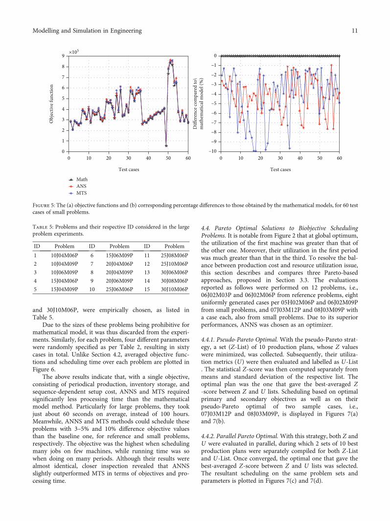
and 30J10M06P, were empirically chosen, as listed inTable 5.

Due to the sizes of these problems being prohibitive formathematical model, it was thus discarded from the experi-ments. Similarly, for each problem, four different parameterswere randomly specified as per Table 2, resulting in sixtycases in total. Unlike Section 4.2, averaged objective func-tions and scheduling time over each problem are plotted inFigure 6.

The above results indicate that, with a single objective,consisting of periodical production, inventory storage, andsequence-dependent setup cost, ANNS and MTS requiredsignificantly less processing time than the mathematicalmodel method. Particularly for large problems, they tookjust about 60 seconds on average, instead of 100 hours.Meanwhile, ANNS and MTS methods could schedule theseproblems with 3–5% and 10% difference objective valuesthan the baseline one, for reference and small problems,respectively. The objective was the highest when schedulingmany jobs on few machines, while running time was sowhen doing on many periods. Although their results werealmost identical, closer inspection revealed that ANNSslightly outperformed MTS in terms of objectives and pro-cessing time.

4.4. Pareto Optimal Solutions to Biobjective SchedulingProblems. It is notable from Figure 2 that at global optimum,the utilization of the first machine was greater than that ofthe other one. Moreover, their utilization in the first periodwas much greater than that in the third. To resolve the bal-ance between production cost and resource utilization issue,this section describes and compares three Pareto-basedapproaches, proposed in Section 3.3. The evaluationsreported as follows were performed on 12 problems, i.e.,06J02M03P and 06J02M06P from reference problems, eightuniformly generated cases per 05H02M06P and 06J02M09Pfrom small problems, and 07J03M12P and 08J03M09P witha case each, also from small problems. Due to its superiorperformances, ANNS was chosen as an optimizer.

4.4.1. Pseudo-Pareto Optimal. With the pseudo-Pareto strat-egy, a set (Z‐List) of 10 production plans, whose Z valueswere minimized, was collected. Subsequently, their utiliza-tion metrics (U) were then evaluated and labelled as U‐List. The statistical Z-score was then computed separately frommeans and standard deviation of the respective list. Theoptimal plan was the one that gave the best-averaged Z-score between Z and U lists. Scheduling based on optimalprimary and secondary objectives as well as on theirpseudo-Pareto optimal of two sample cases, i.e.,07J03M12P and 08J03M09P, is displayed in Figures 7(a)and 7(b).

4.4.2. Parallel Pareto Optimal.With this strategy, both Z andU were evaluated in parallel, during which 2 sets of 10 bestproduction plans were separately compiled for both Z‐Listand U‐List. Once converged, the optimal one that gave thebest-averaged Z-score between Z and U lists was selected.The resultant scheduling on the same problem sets andparameters is plotted in Figures 7(c) and 7(d).

Test cases

MathANSMTS

Obj

ectiv

e fun

ctio

n×105

9

8

7

6

5

4

3

2

1

00 10 20 30 40 50 60

Test cases

Diff

eren

ce co

mpa

red

to\

mat

hem

atic

al m

odel

(%)

0

–1

–2

–3

–4

–5

–6

–7

–8

–9

–100 10 20 30 40 50 60

Figure 5: The (a) objective functions and (b) corresponding percentage differences to those obtained by the mathematical models, for 60 testcases of small problems.

Table 5: Problems and their respective ID considered in the largeproblem experiments.

ID Problem ID Problem ID Problem

1 10J04M06P 6 15J06M09P 11 25J08M06P

2 10J04M09P 7 20J04M06P 12 25J10M06P

3 10J06M09P 8 20J04M09P 13 30J06M06P

4 15J04M06P 9 20J06M09P 14 30J08M06P

5 15J04M09P 10 25J06M06P 15 30J10M06P


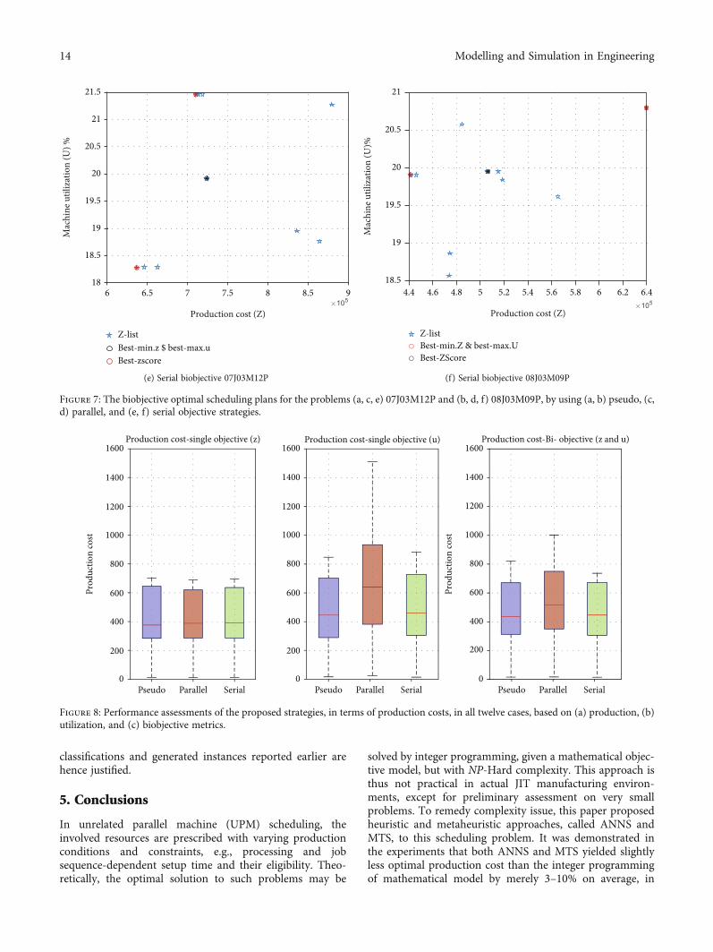
4.4.3. Serial Pareto Optimal. This strategy was similar to theabove strategies, except that after the primary objective wasevaluated for each plan, it would then be evaluated by thesecondary one. The plan with the best primary scores wouldonly be stored in a candidate list, only if its secondary scorewas higher than an acceptable threshold. The resulted sched-uling on the same problem sets and parameters is displayedin Figures 7(e) and 7(f).

In terms of efficiency for all twelve cases, the pseudo-Pareto strategy took the least computing time of 403 secondson average (ranging between 79 and 1021 sec.), followed byserial and parallel of 536 seconds (ranging between 92 and1820 sec) and 887 seconds (ranging between 164 and2384 sec), respectively.

To assess the performance of the proposed strategies,Box-Whisker plots of resultant production costs in all twelvecases, based on production (left), utilization (middle), andbiobjective (right) metrics, are illustrated in Figure 8. It isclearly seen that, when aiming at minimizing productioncost (Z), the primary objective was generally low, while max-imizing machine utilization (U) slightly raised it, but partic-ularly in parallel cases, to greater extent (e.g., at almost100%). On the other hand, scheduling with biobjective (Zand U) model resulted in balanced cost versus utilization,while maintaining relatively low overall costs. Nonetheless,marginal decrease in this balance is noticeable with the par-allel Pareto strategy.

Similar analyses can be made regarding machine utiliza-tion. In Figure 9, Box-Whisker plots of resultant machineutilization in the same cases are plotted. It is clearly seenthat, with utilization being optimized, their values tendedto be a little higher than when focusing primarily on produc-tion cost. However, the biobjective model well balanced them,especially when taking pseudo-Pareto-based approach.

Further analyses on individual cases are reported inFigure 10. It revealed that, for small problems, both metrics

remained similar regardless of an approach taken, except,however, as problems got larger, when the pseudo- and par-allel Pareto-based approaches resulted in lower productioncost and higher utilization, respectively. The graphs also sug-gest that the serial Pareto-based approach was the best com-promise on these metrics.

4.5. Assessments on the Number of Problem Instances. Whenformulating the reference problems, we devised exhaustivecombinations of scheduling {6, 9} jobs on {2, 3, 6} machineswithin {3, 6} periods, resulting in 12 cases. But only 3instances were executed. In addition, for small problems,out of 24 combinations of {5, 6, 7, 8} jobs on {6, 9, 12}machines within {2, 3} periods, 10 cases were selected. Foreach case, 6 production parameters (i.e., P, R, S, D, E, G,and O) were randomly generated as per Table 2, resultingin 60 instances being analyzed. Likewise, for large problems,a total of 15 cases, each with 6 production parameters,resulted in 90 instances being considered. Finally, on evalu-ating Pareto optimization, a total of 12 instances were drawnfrom references and small problems. Accordingly, therewere in total 153 different scheduling instances involved inthe above experiments.

Nonetheless, to elucidate that the number of instanceswas sufficient to draw conclusions, an experiment on addi-tional cases, i.e., 06J04M10P, 06J04M15P, 09J04M15P, and09J06M10P, each with 4 parameter settings, was performedby using ANN and MTS algorithms, in turn. Their resultantobjectives were computed and then averaged over a givenproblem. The Box-Whisker plots comparing both algo-rithms and four cases are illustrated in Figure 11.

It is evident that regardless of manufacturing parametersand algorithms, each problem case exhibited similar objec-tives, i.e., as small as about 0.6–3.5% percent deviations. Thisimplies that its performance is dependent only on the prob-lem sizes but not variations over instances. The problem

Obj

ectiv

e val

ueAverage objective value Average run-time

Run

time (

sec)

Problem IDProblem ID

10 4

3.5

3

2.5

2

1.5

1

0.5

0

9

8

7

6

5

4

3

2

ANSMTS

0 2 4 6 8 10 12 14 16 0 2 4 6 8 10 12 14 16

×105 ×104

Figure 6: The (a) average objective functions and (b) processing time for 15 selected large problems, scheduled by ANNS and MTSmethods.


Production Cost (Z)

Mac

hine

Util

izat

ion

(U) %

32

30

28

26

24

22

20

180.6 0.7 0.8 0.9 1 1.1 1.2 1.3 1.4 1.5 1.6

×106

Z-listU-listBest-min.z $ best-max.uBest-zscore

(a) Pseudo-biobjective 07J03M12P

Mac

hine

util

izat

ion

(u) %

Production cost (z)

36

34

32

30

28

26

24

22

20

180.4 0.6 0.8 1 1.2 1.4 1.6

×105

Z-listU-listBest-min.z $ best-max.uBest-zscore

(b) Pseudo-biobjective 08J03M09P

Production cost (Z)

Mac

hine

util

izat

ion

(U) %

22

21

20

19

18

17

166.5 7 7.5 8 8.5 9 9.5

×105

z-listBest-min.z$ best-max.uBest-zscore

(c) Parallel biobjective 07J03M12P

Mac

hine

util

izat

ion

(U) %

Production cost (Z)

27

26

25

24

23

22

21

20

19

18

174 4.5 5 5.5 6 6.5

×105

Z-list

Best-zscoreBest-min.z $ best-max.u

(d) Parallel biobjective 08J03M09P

Figure 7: Continued.


classifications and generated instances reported earlier arehence justified.

5. Conclusions

In unrelated parallel machine (UPM) scheduling, theinvolved resources are prescribed with varying productionconditions and constraints, e.g., processing and jobsequence-dependent setup time and their eligibility. Theo-retically, the optimal solution to such problems may be

solved by integer programming, given a mathematical objec-tive model, but with NP-Hard complexity. This approach isthus not practical in actual JIT manufacturing environ-ments, except for preliminary assessment on very smallproblems. To remedy complexity issue, this paper proposedheuristic and metaheuristic approaches, called ANNS andMTS, to this scheduling problem. It was demonstrated inthe experiments that both ANNS and MTS yielded slightlyless optimal production cost than the integer programmingof mathematical model by merely 3–10% on average, in

Production cost (Z)

Mac

hine

util

izat

ion

(U) %

21

21.5

20.5

20

19.5

19

18

18.5

6 6.5 7 7.5 8 8.5 9

Best-min.z $ best-max.uBest-zscore

Z-list

(e) Serial biobjective 07J03M12PM

achi

ne u

tiliz

atio

n (U

)%

Production cost (Z)

21

20.5

20

19.5

19

4.4 4.6 4.8

Z-list

Best-ZScoreBest-min.Z & best-max.U

5 5.2 5.4 5.6 5.8 6 6.2 6.418.5

(f) Serial biobjective 08J03M09P

Figure 7: The biobjective optimal scheduling plans for the problems (a, c, e) 07J03M12P and (b, d, f) 08J03M09P, by using (a, b) pseudo, (c,d) parallel, and (e, f) serial objective strategies.

Production cost-single objective (z) Production cost-single objective (u) Production cost-Bi- objective (z and u)1600

1400

1200

1000

800

600

400

200

1600

1400

1200

1000

800

600

400

200

0 0Pseudo Parallel Serial Pseudo Parallel Serial

0Pseudo Parallel Serial

Prod

uctio

n co

st1600

1400

1200

1000

800

600

400

200

Prod

uctio

n co

st

Figure 8: Performance assessments of the proposed strategies, in terms of production costs, in all twelve cases, based on (a) production, (b)utilization, and (c) biobjective metrics.


reference and small problems. Nonetheless, their computingperformance was significantly better. They could completeall the problems well under the one-minute mark, whereastheir counterpart would take days or, for larger problems,unable to compute at all.

Moreover, we also demonstrated that primarily optimiz-ing production cost that consisted of process time and setuptime, and inventory cost, could inevitably result in unbal-anced resource utilization. To resolve this issue, we formu-lated biobjective UPM scheduling model in finite integerdomains. These objectives involved minimizing productioncost and machine utilization under various prescribedresource and production conditions. The final decision was

the policy, assigning a sequence of jobs to UPMs and associ-ate production quantity for a given period. To this end, weproposed the Pareto-based approaches, i.e., pseudo, parallel,and serial ones, where both production cost and utilizationmetrics were considered. Among these variations, their dif-ferences were undiscernible for small problems. However,as problems got larger and more complex, the pseudo-Pareto-based approach appeared to be the best compromisebetween both metrics. In terms of complexity, parallelPareto strategy needed the greatest time to compute,followed by serial and pseudo variants, respectively. Theirfinal solutions were, however, indiscernible in the studiedproblems.

Percent utilization-single objective (z) Percent utilization-single objective (u)40

35

30

25

20

15

10

5

0

Perc

ent u

tiliz

atio

n

Perc

ent u

tiliz

atio

n

Perc

ent u

tiliz

atio

n

Pseudo Parallel Serial Pseudo Parallel Serial Pseudo Parallel Serial

40

35

30

25

20 20

15

10

5

0

40

35

30

25

15

10

5

0

Percent utilization-Bi-objective (z and u)

Figure 9: Performance assessments of the proposed strategies, in terms of percent machine utilization, in all twelve cases, based on (a)production, (b) utilization, and (c) biobjective metrics.

0

200

400

600

800

1000

1200

1 2 3 4 5 6 7 8 9 10 11 12

Prod

uctio

n co

st

Evaluation cases

Production cost in bi-objective strategies

Larger problems

10 11 120

5

10

15

20

25

30

35

40

1 2 3 4 5 6 7 8 9

Perc

ent u

tiliz

atio

n

Evaluation cases

Machine utilization in bi-objective strategies

PseudoParallelSerial

Larger problems

Figure 10: Production cost and machine utilization of involved cases obtained by biobjective strategies.


In perspective, the developed metaheuristic schemescould be used to solve large problems. It was demonstratedin the experiments that optimizing small problems by ANNSand MTS was highly efficient. They gave solutions with assmall deviations from the optimal ones as 3.69% and4.51%, respectively, on average. As the problems becamelarger, both algorithms gave inferior solutions but by nogreater than 5%, compared to those solved by a muchtime-consuming mathematical model. Specifically, depend-ing on initial condition, the computation times were broughtdown from hundreds of hours to a matter of minutes, whenboth optimizers converged to similar outcomes. Further-more, the proposed Pareto approaches to biobjective modelsallowed simultaneously minimizing both production costand machine utilization. In practice, however, it may bepreferable to maximize utilization, while keeping the costlow. To this end, adjustment to the proposed framework istrivial. However, further constraint on the utilizations beinglower than say 80% for all periods is suggested, to preventoverload.

Unlike a previous work [73], which posed the problemson a single machine as a traveling salesman one (TSP), ourwork tackled them on multiple machines as vehicle routingproblem (VRP). Compared with [74], where no setup timeand stochastic process time were assumed, our modelrelieved these constraints and considered deterministic pro-cess time with SDS. As such, our model could be extended toprecedence job shop scheduling, where conditions on previ-ous and next jobs are specified. The developed model isapplicable on both single and parallel machine environ-ments. In the case of single machine, the setup time for aprohibited chain, e.g., from job j to k, on a machine, m,could be set to an extremely high cost so that it will be dis-carded during the optimization. However, this technique

may fail, if the optimizer inserts a job in between, i.e., j, m,then k, in which case multilevel SDS may be needed. Forparallel machine, since our method computes completiontime for each job, order of a chain can be directed by settingits cost, based on the number of completed items for eachjob. For example, in a case where job k must succeed j,unless the number of items processed by job k is less thanthat by job j, then its cost will be set to some high value, toavoid being selected.

Other future directions worth focused on include inves-tigation on soft-computing schemes such as convolutionalneural network (CNN) and validation on more realistic con-ditions, e.g., taking into account unscheduled maintenanceand ad hoc job insertion.

Data Availability

The scheduling problem in Microsoft Excel (.xlsx), resultsobtained from the mathematical model in LINGO (.lgr),and simulation results in MATLAB data (.mat) formats usedto support the findings of this study are available from thecorresponding author upon request.

Conflicts of Interest

The authors declare that there is no conflict of interestregarding the publication of this paper.

Acknowledgments

The authors would like to thank the Institute of Researchand Development (IRD), Suranaree University of Technol-ogy for funding, and faculty members and supporting staffsfrom the Institute of Engineering and Centre for Scientific

5

4.5

4

3.5

3

2.5

5.5

Obj

ectiv

e val

ue

ANN MTS

Test1: 06J04M10P

×105

Var. =6.86+07 Var. =

2.80e+06

ANN MTS

Test2: 06J04M15P

Obj

ectiv

e val

ue

3.5

2.5

3

4

4.5

5

5.5×105

Var. =1.68e+08

Var. =1.54e+08

ANN MTS

Test3: 09J04M15P

5.5

5

4.5

4

3.5

Obj

ectiv

e val

ue

3

2.5

×105

Var. =4.28e+08

Var. =3.02e+08i

5.5

5

4.5

4

3.5

3

2.5

ANN MTS

Test4: 09J06M10P

×105

Var. =3.65e+07

Var. =1.26e+08

Obj

ectiv

e val

ue

Figure 11: Box-Whisker plots comparing the objectives that resulted from ANN and MTS in four different cases.


and Technological Equipment (CSTE) for their contribu-tion, critiques, advice, and supports in preparing and con-ducting this study.

References

[1] V. Kayvanfar, M. Zandieh, and E. Teymourian, “An intelligentwater drop algorithm to identical parallel machine schedulingwith controllable processing times: a just-in-time approach,”Computational and Applied Mathematics, vol. 36, no. 1,pp. 159–184, 2017.

[2] M. M. Ahmadian, A. Salehipour, and T. C. E. Cheng, “Ameta-heuristic to solve the just-in-time job-shop scheduling prob-lem,” European Journal of Operational Research, vol. 288,no. 1, pp. 14–29, 2021.

[3] G. I. Adamopoulos and C. P. Pappis, “Scheduling under acommon due-data on parallel unrelated machines,” EuropeanJournal of Operational Research, vol. 105, no. 3, pp. 494–501,1998.

[4] K. C. Ying and S. W. Li, “Unrelated parallel machine schedul-ing with sequence- and machine-dependent setup times anddue date constraints,” International Journal of InnovativeComputing, Information and Control, vol. 8, no. 1, pp. 1–19,2012.

[5] J. R. Zeidi and S. MohammadHosseini, “Scheduling unrelatedparallel machines with sequence-dependent setup times,”International Journal of Advanced Manufacturing Technology,vol. 81, no. 9-12, pp. 1487–1496, 2015.

[6] V. Suresh and D. Chaudhuri, “Bicriteria scheduling problemfor unrelated parallel machines,” Computers and IndustrialEngineering, vol. 30, no. 1, pp. 77–82, 1996.

[7] S. Zdrzalka, “Preemptive scheduling with release dates, deliv-ery times and sequence independent setup times,” EuropeanJournal of Operational Research, vol. 76, no. 1, pp. 60–71, 1994.

[8] S. Gawiejnowicz, “Scheduling deteriorating jobs subject to jobor machine availability constraints,” European Journal ofOperational Research, vol. 180, no. 1, pp. 472–478, 2007.

[9] Y. H. Lee and M. Pinedo, “Scheduling jobs on parallelmachines with sequence-dependent setup times,” EuropeanJournal of Operational Research, vol. 100, no. 3, pp. 464–474,1997.

[10] S. Wang, M. Kurz, S. J. Mason, and E. Rashidi, “Two-stagehybrid flow shop batching and lot streaming with variable sub-lots and sequence-dependent setups,” International Journal ofProduction Research, vol. 57, no. 22, pp. 6893–6907, 2019.

[11] C. C. Han, K. G. Shin, and J. Wu, “A fault-tolerant schedulingalgorithm for real-time periodic tasks with possible softwarefaults,” IEEE Transactions on Computers, vol. 52, no. 3,pp. 362–372, 2003.

[12] P. Wu and B. S. Manjunath, “Adaptive nearest neighboursearch for relevance feedback in large image databases,” in Pro-ceedings of the ninth ACM international conference on Multi-media, pp. 89–97, Ottawa, Canada, October 2001.

[13] R. Alonso, J. A. Bloom, H. Li, and C. Basu, “An adaptive near-est neighbour search for a parts acquisition ePortal,” in Pro-ceedings of the ninth ACM SIGKDD international conferenceon Knowledge discovery and data mining, pp. 693–698, Wash-ington, D.C, August 2003.

[14] Z. C. Zhu, K. M. Ng, and H. L. Ong, “A modified tabu searchalgorithm for cost-based job shop problem,” Journal of theOperational Research Society, vol. 61, no. 4, pp. 611–619, 2010.

[15] A. Kharrousheh, S. Abdullah, and M. Z. A. Nazri, “A modifiedtabu search approach for the clustering problem,” Journal ofApplied Sciences, vol. 11, no. 9, 2011.

[16] M. Fera, R. Macchiaroli, F. Fruggiero, and A. Lambiase, “Amodified tabu search algorithm for the single-machine sched-uling problem using additive manufacturing technology,”International Journal of Industrial Engineering Computations,vol. 11, no. 3, 2020.

[17] L. Cheng Hao, W. Yan Hong, Q. J. Wei, D. W. Zhao, andS. Rui, “Product service scheduling problem with servicematching based on tabu search method,” Journal of AdvancedTransportation, vol. 2020, Article ID 5748680, 9 pages, 2020.

[18] J. Blazewicz, K. H. Ecker, E. Pesch, G. Schmidt, and J. Weglarz,Scheduling Computers and Manufacturing Processes, Springer,Berlin, 1996.

[19] R. Slowinski, “Production scheduling on parallel machinessubject to staircase demands,” Engineering Costs and Produc-tion Economics, vol. 14, no. 1, pp. 11–17, 1988.

[20] G. Centeno and R. L. Armacost, “Parallel machine schedulingwith release time and machine eligibility restrictions,” Com-puters & Industrial Engineering, vol. 33, no. 1-2, pp. 273–276,1997.

[21] K. R. Baker, Introduction to Sequencing and Scheduling, Wileyand Sons, New York, 1974.

[22] A. Chassein and A. Kinscherff, “Complexity of strict robustinteger minimum cost flow problems: an overview and furtherresults,” Computers and Operations Research, vol. 104,pp. 228–238, 2019.

[23] A. A. Anwar and D. Clarke, “Irrigation scheduling usingmixed-integer linear programming,” Journal of Irrigation andDrainage Engineering, vol. 127, no. 2, pp. 63–69, 2001.

[24] J. Kim and K. Kim, “Dynamic programming for scalable just-in-time economic dispatch with non- convex constraints andanytime participation,” International Journal of ElectricalPower & Energy Systems, vol. 123, no. 1, article 106217, 2020.

[25] M. Bihari and P. V. Kane, “Evaluation and improvement ofmakespan time of flexible job shop problem using various dis-patching rules-a case study,” in Advances in Mechanical Engi-neering, Springer, Singapore, 2020.

[26] G. A. Süer, F. Pico, and A. Santiago, “Identical machine sched-uling to minimize the number of tardy jobs when lot- splittingis allowed,” Computers and Industrial Engineering, vol. 33,no. 1-2, pp. 277–280, 1997.

[27] J. C. Ho and Y. L. Chang, “Minimizing the number of tardyjobs form parallel machines,” European Journal of OperationalResearch, vol. 84, no. 2, pp. 343–355, 1995.

[28] D. Bai, H. Xue, L. Wang, C. C. Wu, W. C. Lin, and D. H.Abdulkadir, “Effective algorithms for single-machinelearning-effect scheduling to minimize completion-time-based criteria with release dates,” Expert Systems with Applica-tions, vol. 156, no. 1, article 113445, 2020.

[29] D. W. Kim, K. H. Kim, W. Jang, and F. Frank Chen, “Unre-lated parallel machine scheduling with setup times using sim-ulated annealing,” Robotics and Computer-IntegratedManufacturing, vol. 18, no. 3-4, pp. 223–231, 2002.

[30] M. Woolway and T. Majozi, “A novel metaheuristic frame-work for the scheduling of multipurpose batch plants,” Chem-ical Engineering Science, vol. 192, no. 1, pp. 678–687, 2018.

[31] Z. Tong, L. Ning, and S. Debao, “Genetic algorithm for vehiclerouting problem with time window with uncertain vehiclenumber,” in Fifth World Congress on Intelligent Control and


Automation (IEEE Cat. No. 04EX788), pp. 2846–2849, Hang-zhou, China, 2004.

[32] S. Prabu, K. Karthik, J. V. Rayudu, and D. G. Krishnan, “Opti-mization of machining parameters in wire EDM of EN24steel,” International Journal of Mechanical and ProductionEngineering Research and Development, vol. 7, no. 6,pp. 359–364, 2017.

[33] B. Zheng, Y. F. Li, and H. Z. Huang, “Aeroengine fault diagno-sis method based on optimized supervised Kohonen network,”Journal of Donghua University, vol. 32, no. 16, pp. 1029–1033,2015.

[34] P. Horkaew and G. Z. Yang, “Construction of 3D dynamic sta-tistical deformable models for complex topological shapes,” inMedical Image Computing and Computer-Assisted Interven-tion – MICCAI 2004, Springer, Berlin, Heidelberg, 2004.

[35] P. Horkaew and S. Puttinaovarat, “Entropy-based fusion ofwater indices and DSM derivatives for automatic water sur-faces extraction and flood monitoring,” ISPRS InternationalJournal of Geo-Information, vol. 6, no. 10, p. 301, 2017.

[36] S. Bekiros, J. A. Hernandez, S. Hammoudeh, and D. K.Nguyen, “Multivariate dependence risk and portfolio optimi-zation: an application to mining stock portfolios,” ResourcesPolicy, vol. 46, no. P2, pp. 1–11, 2015.

[37] R. M. Karp, Reducibility among Combinatorial Problems:Complexity of Computer Computations, Plenum Press, NewYork, 1972.

[38] P. He, “Optimization and simulation of remanufacturingproduction scheduling under uncertainties,” InternationalJournal of Simulation Modelling, vol. 17, no. 4, pp. 734–743, 2018.

[39] S. Rajakumar, V. P. Arunachalam, and V. Selladurai, “Work-flow balancing in parallel machine scheduling with precedenceconstraints using genetic algorithm,” Journal of Manufactur-ing Technology Management, vol. 17, no. 2, pp. 239–254, 2006.

[40] S. Tian, T. Wang, L. Zhang, and X. Wu, “Real-time shop floorscheduling method based on virtual queue adaptive control:algorithm and experimental results,” Measurement (Lond),vol. 147, no. 1, 2019.

[41] D. M. Ryan, C. Hjorring, and F. Glover, “Extensions of thepetal method for vehicle routeing,” The Journal of the Opera-tional Research Society, vol. 44, no. 3, pp. 289–296, 1993.

[42] J. Renaud and F. F. Boctor, “A sweep-based algorithm for thefleet size and mix vehicle routing problem,” European Journalof Operational Research, vol. 140, no. 3, pp. 618–628, 2002.

[43] C. Prins, P. Lacomme, and C. Prodhon, “Order-first split-second methods for vehicle routing problems: a review,”Transportation Research Part C, vol. 40, no. 1, pp. 179–200,2014.

[44] P. Hansen and N. Mladenović, “Variable neighborhood searchfor the _p_ -median,” Location Science, vol. 5, no. 4, pp. 207–226, 1997.

[45] P. Hansen and N. Mladenović, “Variable neighborhoodsearch,” in Search Methodologies, E. K. Burke and G. Kendall,Eds., Springer, Boston, MA, 2005.

[46] L. Shen, M. F. Tasgetiren, H. Öztop, L. Kandiller, and L. Gao,“A general variable neighborhood search for the noIdle flow-shop scheduling problem with makespan criterion,” in 2019IEEE Symposium Series on Computational Intelligence (SSCI),pp. 1684–1691, Xiamen, China, December 2019.

[47] B. Hu, M. Leitner, and G. R. Raidl, “Combining variable neigh-borhood search with integer linear programming for the gen-

eralized minimum spanning tree problem,” Journal ofHeuristics, vol. 14, no. 5, pp. 473–499, 2008.

[48] J. Kluabwang, D. Puangdownreong, and S. Sujitjorn, “Multi-path adaptive tabu search for a vehicle control problem,” Jour-nal of Applied Mathematics, vol. 2012, Article ID 731623, 20pages, 2012.

[49] S. Bechikh, N. Belgasmi, L. B. Said, and K. Ghédira, “PHC-NSGA-II: a novel multi-objective memetic algorithm for con-tinuous optimization,” in 008 20th IEEE International Confer-ence on Tools with Artificial Intelligence, vol. 1, pp. 180–189,Dayton, OH, USA, November 2008.

[50] C. Dandois, Multi-Objective Evolutionary Concept LearnerSystem, [M.S. Thseis], University of Namur, 2009.

[51] N. Srinivas and K. Deb, “Multiobjective function optimizationusing nondominated sorting genetic algorithms,” EvolutionaryComputation, vol. 2, no. 3, pp. 221–248, 1995.

[52] D. E. Goldberg, B. Korb, and K. Deb, “Messy genetic algo-rithms: motivation, analysis, and first results,” Complex Sys-tems, vol. 3, no. 5, pp. 493–530, 1989.

[53] C. M. Fonseca and P. J. Fleming, “Multiobjective optimizationand multiple constraint handling with evolutionary algo-rithms. I. A unified formulation,” IEEE Transactions on Sys-tems, Man, and Cybernetics-Part A: Systems and Humans,vol. 28, no. 1, pp. 26–37, 1998.

[54] A. J. Ruiz-Torres, F. J. López, and J. C. Ho, “Scheduling uni-form parallel machines subject to a secondary resource to min-imize the number of tardy jobs,” European Journal ofOperational Research, vol. 179, no. 2, pp. 302–315, 2007.

[55] D. W. Kim, D. G. Na, and F. F. Chen, “Unrelated parallelmachine scheduling with setup times and a total weighted tar-diness objective,” Robotics and Computer-IntegratedManufacturing, vol. 19, no. 1-2, pp. 173–181, 2003.

[56] E. B. Edis and C. Oguz, “Parallel machine scheduling with flex-ible resources,” Computers and Industrial Engineering, vol. 63,no. 2, pp. 433–447, 2012.

[57] S. Polyakovskiy and R. M. Hallah, “Minimizing weighted ear-liness and tardiness on parallel machines using a multi-agentsystem,” Operations Research Proceedings, Springer, 2012.

[58] V. Kayvanfar, I. Mahdavi, and G. H. M. Komaki, “A drastichybrid heuristic algorithm to approach to JIT policy consider-ing controllable processing times,” Journal of AdvancedManufacturing Technology, vol. 69, no. 1-4, pp. 257–267, 2013.

[59] Z. Zhang, L. Zheng, N. Li, W. Wang, S. Zhong, and K. Hu,“Minimizing mean weighted tardiness in unrelated parallelmachine scheduling with reinforcement learning,” Computersand Operations Research, vol. 39, no. 7, pp. 1315–1324, 2012.

[60] V. Kayvanfar and E. Teymourian, “Hybrid intelligent waterdrops algorithm to unrelated parallel machines schedulingproblem: a just-in-time approach,” International Journal ofProduction Research, vol. 52, no. 19, pp. 5857–5879, 2014.

[61] G. V. Kayvanfar, E. Teymourian, and K. Mashhadi Alizadeh,“Intelligent water drops algorithm on parallel machines sched-uling,” in the Proceedings of IEEE 5th International Conferenceon Industrial Engineering and Operations Management(IEOM), Dubai, UAE, 2015.

[62] J. Lin and K. C. Ying, “ABC-based manufacturing schedulingfor unrelated parallel machines with machine-dependent andjob sequence-dependent setup times,” Computers & Opera-tions Research, vol. 51, pp. 172–181, 2014.

[63] I. V. Kayvanfar, G. H. M. Komaki, A. Aalaei, and M. Zandieh,“Minimizing total tardiness and earliness on unrelated parallel


machines with controllable processing times,” Computers &Operations Research, vol. 41, pp. 31–43, 2014.

[64] K. M. Afzalirad and J. Rezaeian, “Resource-constrained unre-lated parallel machine scheduling problem with sequencedependent setup times, precedence constraints and machineeligibility restrictions,” Computers & Industrial Engineering,vol. 98, pp. 40–52, 2016.

[65] H. Soleimani, H. Ghaderi, P. W. Tsai, N. Zarbakhshnia, andM. Maleki, “Scheduling of unrelated parallel machines consid-ering sequence-related setup time, start time-dependent dete-rioration, position-dependent learning and powerconsumption minimization,” Journal of Cleaner Production,vol. 249, article 119428, 2020.

[66] D. O. Shahvari and R. Logendran, “A bi-objective batch pro-cessing problem with dual-resources on unrelated- parallelmachines,” Applied Soft Computing, vol. 61, pp. 174–192,2017.

[67] B. Shahidi-Zadeh, R. Tavakkoli-Moghaddam, A. Taheri-Moghadam, and I. Rastgar, “Solving a bi-objective unrelatedparallel batch processing machines scheduling problem: acomparison study,” Computers & Operations Research,vol. 88, pp. 71–90, 2017.

[68] B. Yepes-Borrero, F. Perea, R. Ruiz, and F. Villa, “Bi-objectiveparallel machine scheduling with additional resources duringsetups,” European Journal of Operational Research, vol. 292,no. 2, pp. 443–455, 2021.

[69] F. Kolahan and V. Kayvanfar, “A heuristic algorithm approachfor scheduling of multi-criteria unrelated parallel machines,”World, Academy of Science, Engineering and Technology,vol. 59, pp. 102–105, 2009.

[70] M. H. F. Zarandi and V. Kayvanfar, “A bi-objective identicalparallel machine scheduling problem with controllable pro-cessing times: a just-in-time approach,” International Journalof Advanced Manufacturing Technology, vol. 77, no. 1-4,pp. 545–563, 2015.

[71] Y. Jin and B. Sendhoff, “Pareto-based multiobjective machinelearning: an overview and case studies,” EEE Transactions onSystems, Man, and Cybernetics, Part C (Applications andReviews), vol. 38, no. 3, pp. 397–415, 2008.

[72] M. Afzalirad and J. Rezaeian, “Design of high-performinghybrid meta-heuristics for unrelated parallel machine schedul-ing with machine eligibility and precedence constraints,” Engi-neering Optimization, vol. 48, no. 4, pp. 706–726, 2015.

[73] N. Xie and N. Chen, “Flexible job shop scheduling problemwith interval grey processing time,” Applied Soft Computing,vol. 70, pp. 513–524, 2018.

[74] E. Balas, N. Simonetti, and A. Vazacopoulos, “Job shop sched-uling with setup times, deadlines and precedence constraints,”Journal of Scheduling, vol. 11, no. 4, pp. 253–262, 2008.


Documents

Biobjective Scheduling for Joint Parallel Machines with