Embed Size (px)
Citation preview
Natural England Joint Publication JP039
Biodiversity Metric 3.0
Auditing and accounting for biodiversity
USER GUIDE
First published 7th July 2021
www.gov.uk/natural-england

Further information
Natural England evidence can be downloaded from our Access to Evidence Catalogue. For more information about Natural England and our work see Gov.UK. For any queries contact the Natural England Enquiry Service on 0300 060 3900 or e-mail [email protected] .
Copyright
This report is published by Natural England under the Open Government Licence - OGLv3.0 for public sector information. You are encouraged to use, and reuse, information subject to certain conditions. For details of the licence visit Copyright. Natural England photographs are only available for non-commercial purposes. If any other information such as maps or data cannot be used commercially this will be made clear within the report.
ISBN 978-1-78354-778-4
© Natural England and other parties 2021
Biodiversity metric 3.0 – User Guide
1
Citation
STEPHEN PANKS A, NICK WHITE A, AMANDA NEWSOME A, JACK POTTER A, MATT
HEYDON A, EDWARD MAYHEW A, MARIA ALVAREZ A, TRUDY RUSSELL A, SARAH J.
SCOTT B, MAX HEAVER C, SARAH H. SCOTT C, JO TREWEEK D, BILL BUTCHER E and
DAVE STONE A 2021. Biodiversity metric 3.0: Auditing and accounting for biodiversity –
User Guide. Natural England.
A – Natural England, B – Environment Agency, C – Department for Environment, Food and
Rural Affairs, D – Treweek Environmental Consultants Ltd, E – eCountability Ltd
Acknowledgements
The Technical Steering Group wishes to acknowledge the personal contribution of the
late Rachel Hoskin
Biodiversity metric 3.0 is the culmination of more than 14-years’ work to develop a practical
metric to measure gains and losses of biodiversity in England. It builds on the model first
proposed in the scoping study commissioned by Defra in 2008 (Treweek et al., 2009)1,
which was further developed to incorporate scores for habitat distinctiveness and condition
(Treweek J., Butcher B. and Temple H (2010)2 and used by Defra for their biodiversity offset
pilots (Defra, 2012)3 . It has been shaped by the knowledge and experience gained across a
variety of different sectors since the offset pilots and the launch, in 2019, of a beta test
version, biodiversity metric 2.0 (Crosher et al., 2019)4.
The development of Biodiversity metric 3.0 would not have been possible without the
considerable effort of a great many people who have shared their experience through
workshops, correspondence and conversation. The authors would like to acknowledge the
help, support and input of:
Julia Baker (Balfour Beatty), Tom Butterworth and Jonny Miller (WSP), David Lowe
(Warwickshire County Council), Rachel Hackett (The Wildlife Trusts), Richard Hellier
(Forestry Commission), Louise Martland (Environment Bank), David Prys-Jones (HS2 Ltd),
Philippa Richards (HS2 Ltd), Andy Fairburn (BBOWT), John Simmons (AECOM), Jack
Rhodes (RSPB), Robert Wolton (Ecological Consultant), Barry Wright (Dryad Ecology),
Louise Clarke (Berkeley Group), Samantha Davenport (Greater London Authority), Jon
Stokes (Tree Council) Claire Gregory (DfT) and Lauren Moore (Defra).
1 DEFRA. 2009. Scoping study for the design and use of biodiversity offsets in an English Context. Written by Jo Treweek with contributions from Kerry ten Kate, Bill Butcher, Orlando Venn, Lincoln Garland, Mike Wells, Dominic Moran and Stewart Thompson. Defra, London. 2 TREWEEK J., BUTCHER B. & TEMPLE H (2010) Biodiversity offsets: possible methods for measuring biodiversity losses and gains for use in the UK. CIEEM In Practice 69, pp29-32.Available at Researchgate 3 DEFRA. 2012. Biodiversity offsetting pilots. Technical paper: the metric for the biodiversity offsetting pilot in England. Defra. March 2012. https://www.gov.uk/government/collections/biodiversity-offsetting 4 The Biodiversity Metric 2.0 - JP029 (naturalengland.org.uk)
Biodiversity metric 3.0 – User Guide
2
Current and former Natural England colleagues: Isabel Alonso, Corrie Bruemmer, Marion
Bryant, Sean Cooch, Kathleen Covill, Alistair Crowle, Iain Diack, Jeff Edwards, Emma
Goldberg, Ruth Hall, Richard Jefferson, Charlotte Johnson, Michael Knight, Chris Mainstone,
Dave Martin, Frances McCullagh, Suzanne Perry, James Phillips, Clare Pinches, Sue Rees,
Graham Weaver and Jon Webb.
Environment Agency colleagues: Phil Belfield, Chris Catling, Dominic Coath, Andrew
Crawford, Judy England, Caroline Essery, Ben Green, Richard Jeffries, Pam Nolan, Tom
Reid and Graham Scholey. Also, with thanks to Angela Gurnell (Queen Mary University of
London) and Lucy Shuker (Cartographer Studios ltd.).
Forestry Commission colleagues: Jane Hull, Neil Riddle and Jim Smith
Our thanks also to Sam Arthur (Associate Ecologist and Biodiversity Net Gain Specialist at
FPCR Environment and Design Ltd) for his significant input into the development of the
Calculation Tool.
Finally, our thanks to all the various workshop attendees and the people who took the time to
provide us with feedback and advice along the way.
The UK Habitat Classification System is used under licence from UKHab Ltd. Please see https://ukhab.org/ for further details about the UK Habitat Classification System.
Users should refer to https://ukhab.org/ for the published definitions and detailed methodologies on the recording of habitats.
Image credits
Box 2-1: Natural England (Matt Heydon, Peter Roworth & Julian Dowse)
Box 8-5: Cartographer Studios Ltd. (Lucy Shuker) & Environment Agency (Neale Hider).
Box 8-6: Environment Agency (Dave Webb)
Biodiversity metric 3.0 – User Guide
3
Contents 3
1: Introduction ....................................................................................................................... 5
Who is this guidance for? .................................................................................................. 5
Why do we need a metric for measuring biodiversity? ....................................................... 5
Scope of biodiversity metric 3.0 ......................................................................................... 5
When can biodiversity metric 3.0 be used?........................................................................ 7
Applying the mitigation hierarchy when using the metric .................................................... 7
2: Summary of how biodiversity metric 3.0 works .................................................................. 9
What the metric measures ................................................................................................. 9
The difference between area and linear habitat units in the metric .................................... 9
How area habitat biodiversity units are calculated ........................................................... 10
Principles and rules for using the metric .......................................................................... 14
3: Data Collection & Preparation for Use in the Metric ......................................................... 20
Introduction...................................................................................................................... 20
Approach ......................................................................................................................... 21
4: How to use the Calculation Tool ...................................................................................... 30
Step 1: Accessing and preparing the tool ..................................................................... 30
Step 2: Baseline (pre-development/intervention) data entry ......................................... 33
Step 3: Post-intervention data entry ............................................................................. 38
Step 4: Off-site data entry ............................................................................................ 42
Step 5: Viewing and interpreting the results ................................................................. 42
Step 6 (optional): Understanding and checking supporting data in the tool .................. 44
5: Detailed description of biodiversity metric 3.0 .................................................................. 45
Components of biodiversity quality .................................................................................. 45
Dealing with risk .............................................................................................................. 50
Biodiversity change scenarios ......................................................................................... 58
6: Area Habitat biodiversity unit calculations ....................................................................... 61
Calculating Area Habitat Biodiversity Units (AHBUs) ....................................................... 64
7: Urban Tree (including street tree) biodiversity unit calculations ....................................... 67
8: Linear habitat biodiversity unit calculations...................................................................... 71
Hedgerows and lines of trees .......................................................................................... 71
Calculating hedgerows and lines of trees Biodiversity Units (HBUs) ............................ 71
Assessing the quality of hedgerows and lines of trees ..................................................... 72
Dealing with risk .............................................................................................................. 75
Rivers and Streams ......................................................................................................... 77
Calculating River and Streams Biodiversity Units (RBUs) ............................................ 77
Assessing the quality of Rivers and Streams ................................................................... 78
Risks ............................................................................................................................... 86
Biodiversity metric 3.0 – User Guide
4
9: Using biodiversity metric 3.0 with other metrics .............................................................. 90
References ......................................................................................................................... 94
Glossary.............................................................................................................................. 97
Biodiversity metric 3.0 – User Guide
5
1: Introduction
Who is this guidance for?
This guidance is for anyone planning to use biodiversity metric 3.0 and anyone who
wants to understand the outputs of the metric. This includes developers who have
commissioned a biodiversity assessment using the metric, communities wanting to
understand the impacts of a local development, and planning authority decision-
makers interpreting metric outputs included in a planning application or land owners
wishing to provide biodiversity units from their sites to others.
In this user guide we explain how to use biodiversity metric 3.0 and describe the
principles and rules underpinning its use.
Why do we need a metric for measuring biodiversity?
1.3 Biodiversity is the term that is used to describe the variety of all life on earth. It
includes all species of animals and plants – and everything else that is alive on our
planet. Habitats are the places in which species live. These species and their habitats
contribute to the ecosystem services that provide substantial benefits to people and
the economy. For example, woodlands and saltmarsh can help prevent flooding
whilst parks and greenspaces make our towns and cities healthier and more
attractive places in which to live and work. Biodiversity is under threat, globally and at
home. Habitats are being damaged or disappearing and species are declining. This is
not just bad news for nature but also for our own health and well-being and that of
future generations. Biodiversity and healthy habitats are vital for a well-functioning
planet, but their value is often not taken into account in decision-making.
Scope of biodiversity metric 3.0
1.4 Biodiversity metric 3.0 is an updated version of the original Defra biodiversity metric5.
It is the culmination of a Defra commissioned project to develop a metric that began
in 2008 (Treweek et al., 2009)6. Biodiversity metric 3.0 builds upon the knowledge
and experience gained across a variety of different sectors since Defra piloted a
provisional metric in 2012 (Defra, 2012) and the consultation and feedback that has
been since a revised beta version, Biodiversity metric 2.07, was launched as a beta
test version in 2019 (Crosher, et al., 2019).This version builds upon the knowledge
and experience gained across a variety of different sectors since the original Defra
biodiversity metric was first launched as part of Defra’s biodiversity offsetting pilots,
5 DEFRA. 2012. Biodiversity offsetting pilots. Technical paper: the metric for the biodiversity offsetting pilot in England. Defra. March 2012. https://www.gov.uk/government/collections/biodiversity-offsetting
6 DEFRA. 2009. Scoping study for the design and use of biodiversity offsets in an English Context. Written by Jo Treweek with contributions from Kerry ten Kate, Bill Butcher, Orlando Venn, Lincoln Garland, Mike Wells, Dominic Moran and Stewart Thompson. Defra, London 2009. Biodiversity Offsets FINAL REPORT Defra 12 May 2009.doc
7 The Biodiversity Metric 2.0 - JP029 (naturalengland.org.uk)
Biodiversity metric 3.0 – User Guide
6
and includes the consultation and feedback that was received on biodiversity metric
2.0.
1.5 Biodiversity metric 3.0 balances robustness with simplicity. It uses habitat as a proxy
for wider biodiversity with different habitat types scored according to their relative
biodiversity value. This value is then adjusted, depending on the condition and
location of the habitat, to calculate ‘biodiversity units’ for that specific project or
development. Biodiversity metric 3.0 incorporates separate calculations for linear
habitats that require a different method of measurement such as hedgerows and lines
of trees, rivers and streams and urban trees.
1.6 Biodiversity metric 3.0 can be used to measure both on-site and off-site biodiversity
changes for a project or development and can be used to measure the change in
biodiversity achieved by different land management interventions. The metric also
accounts for some of the risks associated whenever new habitat is created or existing
habitat is enhanced. The metric calculates the change in biodiversity resulting from a
project or development by subtracting the number of pre-intervention or ‘baseline’
biodiversity units (i.e. those originally existing on-site and off-site) from the number of
post-intervention units (i.e. those projected to be provided after the development or
change in land management). It is important to note that achieving gains in
biodiversity from the calculation does not necessarily mean a development
meets any wider requirements of planning policy or law relating to nature
conservation or biodiversity.
1.7 Biodiversity metric 3.0 only accounts for direct impacts on habitats within the
footprint of a development or project. It has been developed to be a simple
assessment tool and only considers direct impacts on biodiversity through impacts on
habitats Although Natural England acknowledges the importance of considering
indirect impacts these have not been included in the metric.
1.8 The units generated by biodiversity metric 3.0, like all biodiversity unit calculations,
come with a ‘health warning’. The outputs of this metric are not absolute values but
provide a proxy for the relative biodiversity worth of a site pre- and post-intervention.
The quality and reliability of outputs will depend on the quality of the inputs. This user
guide provides advice on how to use the biodiversity unit approach and where and
when it is appropriate for use. The metric is not a substitute for expert ecological
advice. The metric does not override or undermine any existing planning policy
or legislation, including the mitigation hierarchy (see section 1.10 below),
which should always be considered as the metric is applied.
1.9 Biodiversity metric 3.0 does not include species explicitly. Instead, it uses habitat
types as a proxy for the biodiversity ‘value’ of the species communities that make up
those different habitats. The metric does not change existing levels of species
protection and does not replace the processes linked to species protection regimes.
1.10 To simplify and streamline the calculation process, biodiversity metric 3.0 comes with
a free calculation tool8 to calculate biodiversity units. A short user guide9 for the
calculation tool is also available.
8 Biodiversity Metric 3.0 - Auditing and accounting for biodiversity: Calculation tool
9 Biodiversity Metric 3.0 - Auditing and accounting for biodiversity: Calculation tool – short user guide
Biodiversity metric 3.0 – User Guide
7
When can biodiversity metric 3.0 be used?
1.11 Biodiversity metric 3.0, when used with appropriate professional advice and
ecological knowledge, enables biodiversity to be measured in a consistent and robust
way. The metric can be used to inform and improve planning, design, land
management and decision-making.
1.12 It can be used to:
• assess or audit the biodiversity unit value of an area of land
• calculate the losses and gains in biodiversity unit value resulting from changes or actions which affect biodiversity, such as from development or changing the conservation management of a land holding
• predict the likely effectiveness of creating new or enhancing existing habitats
• compare different plan and project proposals for a site allowing more objective assessments of alternative approaches to be made
1.13 The metric can be used throughout all stages of a project or scheme, from site
selection and options assessment through to detailed design. The earlier it is applied
the greater the opportunities for:
• optimising the design to deliver net gains within the project area
• determining whether the project is suitable for application of this metric
• testing whether the outcomes are as expect
1.14 This metric has been designed for application to UK terrestrial and intertidal habitats.
These include freshwater habitats and linear habitat features. It can be applied at a
range of scales from developments of a few houses or land management changes in
individual fields to strategic allocations or entire land holdings.
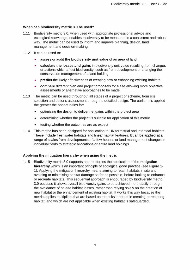
Applying the mitigation hierarchy when using the metric
1.15 Biodiversity metric 3.0 supports and reinforces the application of the mitigation
hierarchy which is an important principle of ecological good practice (see Figure 1-
1). Applying the mitigation hierarchy means aiming to retain habitats in situ and
avoiding or minimising habitat damage so far as possible, before looking to enhance
or recreate habitats. This sequential approach is encouraged by biodiversity metric
3.0 because it allows overall biodiversity gains to be achieved more easily through
the avoidance of on-site habitat losses, rather than relying solely on the creation of
new habitat or the enhancement of existing habitat. It works this way because the
metric applies multipliers that are based on the risks inherent in creating or restoring
habitat, and which are not applicable when existing habitat is safeguarded.
Biodiversity metric 3.0 – User Guide
8
FIGURE 1-1: The Mitigation Hierarchy10
10 Source: adapted from DEFRA, 2018, Net Gain Consultation Proposals. Defra, December 2018. https://consult.defra.gov.uk/land-use/net-gain/supporting_documents/netgainconsultationdocument.pdf (Accessed 20-06-2019)
Biodiversity metric 3.0 – User Guide
9
2: Summary of how biodiversity metric 3.0 works
2.1. This chapter provides an overview of what biodiversity metric 3.0 measures and how,
the key steps in the process and the principles and rules that must be applied. More
detailed explanations of the metric’s functions for frequent or technical users can be
found in subsequent chapters and the Technical Supplement.
What the metric measures
2.2. Biodiversity metric 3.0 uses habitats, the places in which species live, as a proxy to
describe biodiversity. These habitats are converted into ‘biodiversity units’. These
biodiversity units are the ‘currency’ of the metric.
2.3. Biodiversity units are calculated using the size of a parcel11 of habitat and its quality.
The metric uses habitat area (measured in hectares) as its core measurement,
except for linear habitats (hedgerows and lines of trees and rivers and streams)
where habitat length (measured in kilometres) is used.
2.4. To assess the quality of a habitat biodiversity metric 3.0 scores:
a. Habitats of different types, such as woodland or grassland, according to their
relative biodiversity value or distinctiveness. Habitats that are scarce or
declining typically score highly relative to habitats that are more common and
widespread.
b. The condition of a habitat. Scoring the biodiversity value of the habitat
relative to others of the same type.
c. Being ‘better’ and ‘more joined-up’ are important facets of habitats that can
contribute to halting and reversing biodiversity declines12, so the metric also
accounts for whether or not the habitat is sited in an area identified, typically
in a relevant local strategy or plan, as being of strategic significance for
nature.
2.5. Where new habitat is created, or existing habitat is enhanced, the difficulty and
associated risks of doing so are taken into account by biodiversity metric 3.0. If
habitat is created to compensate for losses elsewhere, then the metric also takes
account of its proximity to the site of the losses.
The difference between area and linear habitat units in the metric
2.6. Biodiversity metric 3.0 includes separate calculations for area habitats (such as a
woodland) and linear habitats (such as a hedgerow or stream). This is because
habitat length is a more meaningful measure of linear habitats than their area.
2.7. There are therefore three broad categories of habitats and biodiversity units for which
scores are calculated differently:
11 Parcels are simply distinct portions of each habitat type present.
12Making Space for Nature: a review of England’s wildlife sites and ecological network. Report to Defra (2010)
Biodiversity metric 3.0 – User Guide
10
• Area habitats (such as grasslands, woodlands and mudflats)
• Linear hedgerows and lines of trees
• Linear rivers and streams
2.8. It is an important rule of the metric that the three types of biodiversity units
described above are unique and cannot be summed, traded or converted (Rule
4). When reporting biodiversity gains or losses with the metric, the three different
biodiversity unit types must be reported separately and not summed to give an
overall biodiversity unit value. For example, a scheme would report a gain of 3 area
habitat units, a loss of 1 hedgerow unit and a loss of 1 river unit rather than an overall
combined gain of 1 unit. The separate Calculation Tool provides a simple way of
undertaking all three biodiversity unit calculations.
How area habitat biodiversity units are calculated
2.9. To measure the biodiversity value of habitats it is first necessary to define the site
boundary and then divide it into appropriate habitat parcels as needed. The parcel
size, habitat type and condition of each habitat parcel should then be recorded. The
metric uses widely used classifications13 for categorising habitats.
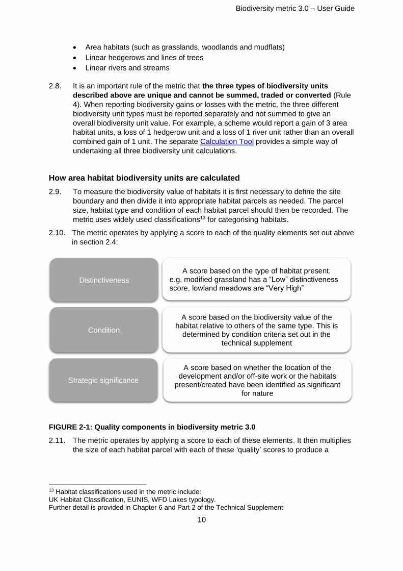
2.10. The metric operates by applying a score to each of the quality elements set out above
in section 2.4:
FIGURE 2-1: Quality components in biodiversity metric 3.0
2.11. The metric operates by applying a score to each of these elements. It then multiplies
the size of each habitat parcel with each of these ‘quality’ scores to produce a
13 Habitat classifications used in the metric include: UK Habitat Classification, EUNIS, WFD Lakes typology. Further detail is provided in Chapter 6 and Part 2 of the Technical Supplement
Distinctiveness
A score based on the type of habitat present. e.g. modified grassland has a “Low” distinctiveness score, lowland meadows are “Very High”
Condition
A score based on the biodiversity value of the habitat relative to others of the same type. This is
determined by condition criteria set out in the technical supplement
Strategic significance
A score based on whether the location of the development and/or off-site work or the habitats
present/created have been identified as significant for nature
Biodiversity metric 3.0 – User Guide
11
number that represents the biodiversity unit value of each habitat parcel (see Box
2-1).
2.12. The user would first calculate the ‘baseline’ or ‘pre-intervention’ value of a site in
biodiversity units before any development or management change has occurred.
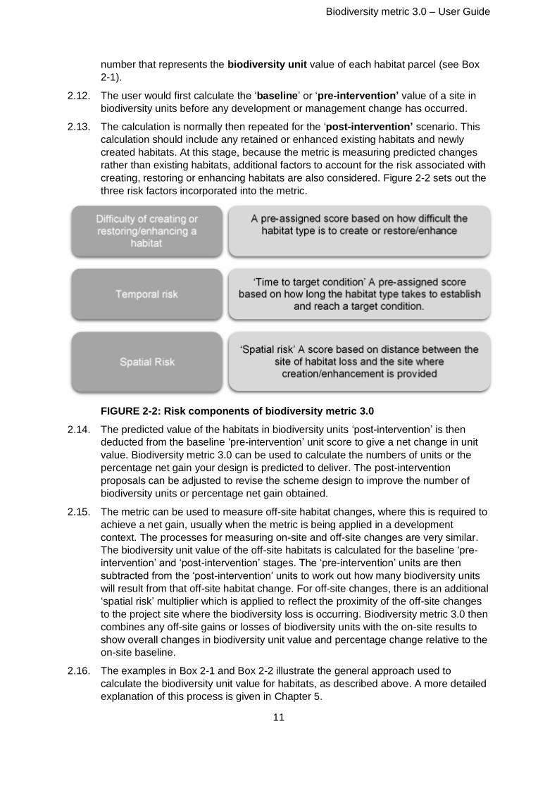
2.13. The calculation is normally then repeated for the ‘post-intervention’ scenario. This
calculation should include any retained or enhanced existing habitats and newly
created habitats. At this stage, because the metric is measuring predicted changes
rather than existing habitats, additional factors to account for the risk associated with
creating, restoring or enhancing habitats are also considered. Figure 2-2 sets out the
three risk factors incorporated into the metric.
FIGURE 2-2: Risk components of biodiversity metric 3.0
2.14. The predicted value of the habitats in biodiversity units ‘post-intervention’ is then
deducted from the baseline ‘pre-intervention’ unit score to give a net change in unit
value. Biodiversity metric 3.0 can be used to calculate the numbers of units or the
percentage net gain your design is predicted to deliver. The post-intervention
proposals can be adjusted to revise the scheme design to improve the number of
biodiversity units or percentage net gain obtained.
2.15. The metric can be used to measure off-site habitat changes, where this is required to
achieve a net gain, usually when the metric is being applied in a development
context. The processes for measuring on-site and off-site changes are very similar.
The biodiversity unit value of the off-site habitats is calculated for the baseline ‘pre-
intervention’ and ‘post-intervention’ stages. The ‘pre-intervention’ units are then
subtracted from the ‘post-intervention’ units to work out how many biodiversity units
will result from that off-site habitat change. For off-site changes, there is an additional
‘spatial risk’ multiplier which is applied to reflect the proximity of the off-site changes
to the project site where the biodiversity loss is occurring. Biodiversity metric 3.0 then
combines any off-site gains or losses of biodiversity units with the on-site results to
show overall changes in biodiversity unit value and percentage change relative to the
on-site baseline.
2.16. The examples in Box 2-1 and Box 2-2 illustrate the general approach used to
calculate the biodiversity unit value for habitats, as described above. A more detailed
explanation of this process is given in Chapter 5.
Biodiversity metric 3.0 – User Guide
12
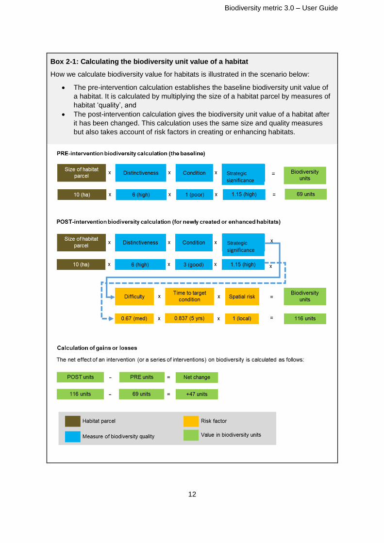
Box 2-1: Calculating the biodiversity unit value of a habitat
How we calculate biodiversity value for habitats is illustrated in the scenario below:
• The pre-intervention calculation establishes the baseline biodiversity unit value of
a habitat. It is calculated by multiplying the size of a habitat parcel by measures of
habitat ‘quality’, and
• The post-intervention calculation gives the biodiversity unit value of a habitat after
it has been changed. This calculation uses the same size and quality measures
but also takes account of risk factors in creating or enhancing habitats.
Strategic
significance
Strategic
significance
Biodiversity metric 3.0 – User Guide
13
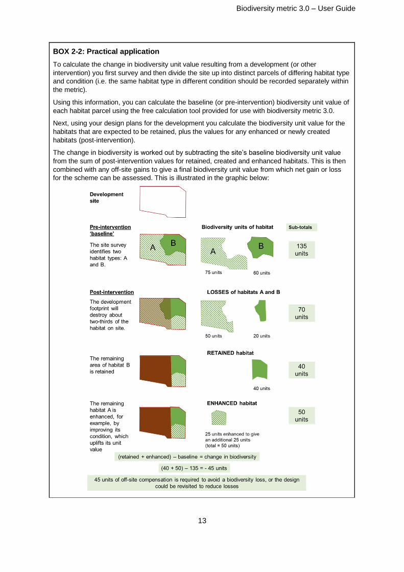
BOX 2-2: Practical application
To calculate the change in biodiversity unit value resulting from a development (or other
intervention) you first survey and then divide the site up into distinct parcels of differing habitat type
and condition (i.e. the same habitat type in different condition should be recorded separately within
the metric).
Using this information, you can calculate the baseline (or pre-intervention) biodiversity unit value of
each habitat parcel using the free calculation tool provided for use with biodiversity metric 3.0.
Next, using your design plans for the development you calculate the biodiversity unit value for the
habitats that are expected to be retained, plus the values for any enhanced or newly created
habitats (post-intervention).
The change in biodiversity is worked out by subtracting the site’s baseline biodiversity unit value
from the sum of post-intervention values for retained, created and enhanced habitats. This is then
combined with any off-site gains to give a final biodiversity unit value from which net gain or loss
for the scheme can be assessed. This is illustrated in the graphic below:
Biodiversity metric 3.0 – User Guide
14
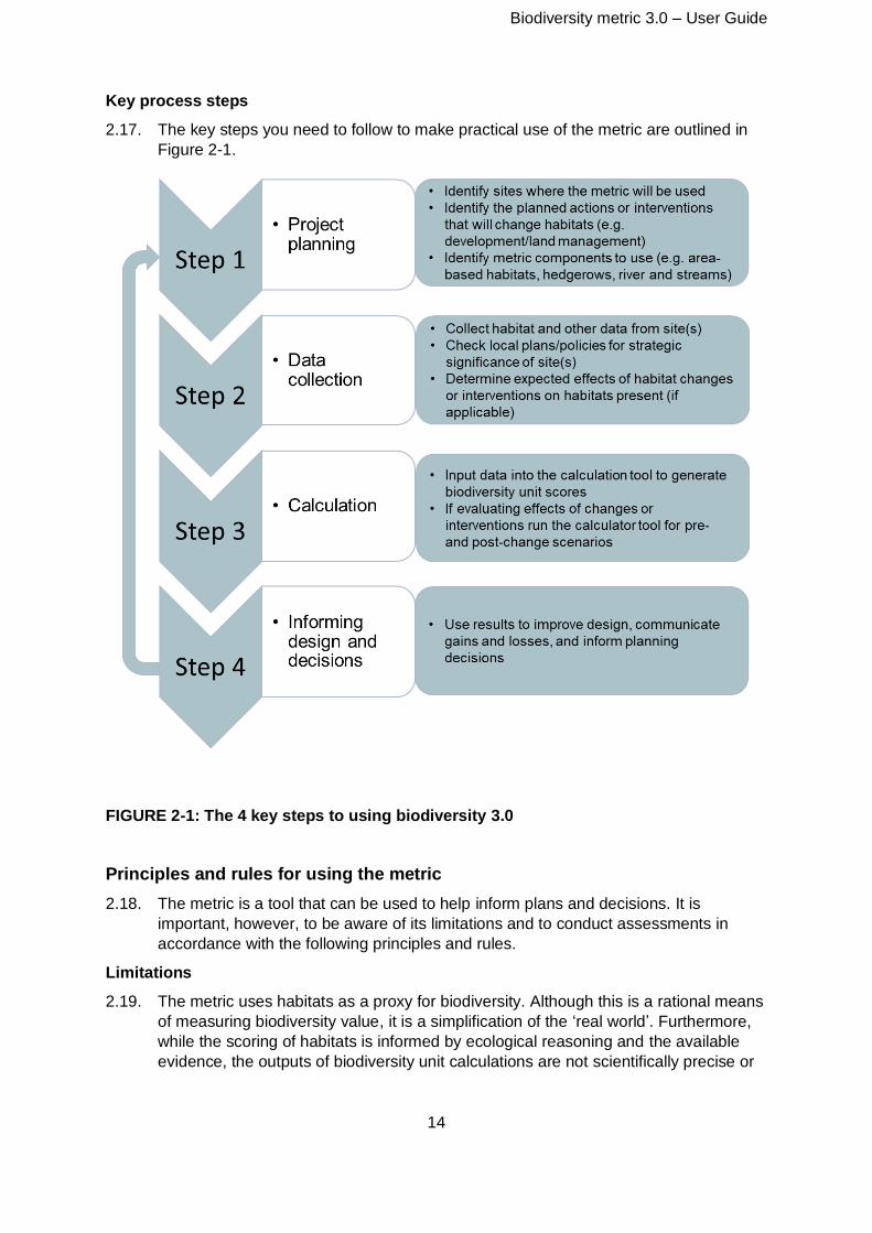
Key process steps
2.17. The key steps you need to follow to make practical use of the metric are outlined in
Figure 2-1.
FIGURE 2-1: The 4 key steps to using biodiversity 3.0
Principles and rules for using the metric
2.18. The metric is a tool that can be used to help inform plans and decisions. It is
important, however, to be aware of its limitations and to conduct assessments in
accordance with the following principles and rules.
Limitations
2.19. The metric uses habitats as a proxy for biodiversity. Although this is a rational means
of measuring biodiversity value, it is a simplification of the ‘real world’. Furthermore,
while the scoring of habitats is informed by ecological reasoning and the available
evidence, the outputs of biodiversity unit calculations are not scientifically precise or
Biodiversity metric 3.0 – User Guide
15
absolute values. The generated biodiversity unit scores are a proxy for the relative
biodiversity worth of a habitat or site.
2.20. The metric and its outputs should therefore be interpreted, alongside ecological
expertise and common sense, as an element of the evidence that informs plans and
decisions. The metric is not a total solution to biodiversity decisions. The metric, for
example, helps you work out how much new or restored habitat is needed to
compensate for a loss of habitat, but it does not tell you the appropriate composition
of plant species to use.
2.21. Assessments should be conducted with regard to a set of key principles and rules.
These are set out below:
Principles
• Principle 1: The metric does not change the protection afforded to
biodiversity. Existing levels of protection afforded to protected species and
habitats are not changed by use of this or any other metric. Statutory
obligations will still need to be satisfied.
• Principle 2: Biodiversity metric calculations can inform decision-making
where application of the mitigation hierarchy and good practice
principles14 conclude that compensation for habitat losses is justified.
• Principle 3: The metric’s biodiversity units are only a proxy for
biodiversity and should be treated as relative values. While it is
underpinned by ecological evidence the units generated by the metric are
only a proxy for biodiversity and, to be of practical use, it has been kept
deliberately simple. The numerical values generated by the metric represent
relative, not absolute, values.
• Principle 4: The metric focuses on typical habitats and widespread
species; important or protected habitats and features should be given
broader consideration.
o Protected and locally important species needs are not considered
through the metric, they should be addressed through existing policy
and legislation.
o Impacts on protected sites (e.g. SSSIs) and irreplaceable habitats are
not adequately measured by this metric. They will require separate
consideration which must comply with existing national and local
policy and legislation. Data relating to these can be entered into the
metric, so as to give an indicative picture of the biodiversity value of
the habitats present on a site, but this should be supported by
bespoke advice.
• Principle 5: The metric design aims to encourage enhancement, not
transformation, of the natural environment. Proper consideration should
14 CIEEM, CIRIA, IEMA. 2016 Biodiversity Net Gain – Good Practice Principles for Development.
https://www.cieem.net/data/files/Publications/Biodiversity_Net_Gain_Principles.pdf
Biodiversity metric 3.0 – User Guide
16
be given to the habitats being lost in favour of higher-scoring habitats, and
whether the retention of less distinctive but well-established habitats may
sometimes be a better option for local biodiversity. Habitat created to
compensate for loss of natural or semi-natural habitat should be of the same
broad habitat type (e.g. new woodland to replace lost woodland) unless there
is a good ecological reason to do otherwise (e.g. to restore a heathland
habitat that was converted to woodland for timber in the past15).
• Principle 6: The metric is designed to inform decisions, not to override
expert opinion. Management interventions should be guided by appropriate
expert ecological advice and not just the biodiversity unit outputs of the
metric. Ecological principles still need to be applied to ensure that what is
being proposed is realistic and deliverable based on local conditions such as
geology, hydrology, nutrient levels, etc. and the complexity of future
management requirements.
• Principle 7: Compensation habitats should seek, where practical, to be
local to the impact. They should aim to replicate the characteristics of the
habitats that have been lost, taking account of the structure and species
composition that give habitats their local distinctiveness. Where possible
compensation habitats should contribute towards nature recovery in England
by creating ‘more, bigger, better and joined up’ areas for biodiversity16.
• Principle 8: The metric does not enforce a mandatory minimum 1:1
habitat size ratio for losses and compensation but consideration should
be given to maintaining habitat extent and habitat parcels of sufficient
size for ecological function. A difference can occur because of a difference
in quality between the habitat impacted and the compensation provided. For
example, if a habitat of low distinctiveness is impacted and is compensated
for by the creation of habitat of higher distinctiveness or better condition, the
area needed to compensate for losses can potentially be less than the area
impacted. However, consideration should be given to whether reducing the
area or length of habitat provided as compensation is an appropriate
outcome.
15 In which case the Open Habitats Policy would need to be followed to ensure suitability of the
proposed change.
16 Making Space for Nature: a review of England’s wildlife sites and ecological network. Report to
Defra (2010)
Biodiversity metric 3.0 – User Guide
17
Rules
• Rule 1: Where the metric is used to measure change, biodiversity unit values
need to be calculated prior to the intervention and post-intervention for all
parcels of land / linear features affected.
• Rule 2: Compensation for habitat losses can be provided by creating new
habitats, or by restoring or enhancing existing habitats.
Measures to enhance existing habitats must provide a significant and
demonstrable uplift in distinctiveness and/or condition to record additional
biodiversity units.
• Rule 3: ‘Trading down’ must be avoided. Losses of habitat are to be
compensated for on a “like for like” or “like for better” basis. New or restored
habitats should aim to achieve a higher distinctiveness and/or condition than
those lost.
Losses of irreplaceable or very high distinctiveness habitat cannot adequately
be accounted for through the metric.
• Rule 4: Biodiversity unit values generated by biodiversity metric 3.0 are
unique to this metric and cannot be compared to unit outputs from version
2.0, the original Defra metric or any other biodiversity metric.
Furthermore, the three types of biodiversity units generated by this metric (for
area, hedgerow and river habitats) are unique and cannot be summed.
• Rule 5: It is not the area/length of habitat created that determines whether
ecological equivalence or better has been achieved but the net change in
biodiversity units. Risks associated with creating or enhancing habitats mean
that it may be necessary to create or enhance a larger area of habitat than
that lost, to fully compensate for impacts on biodiversity.
• Rule 6: Deviations from the published methodology of biodiversity metric 3.0
need to be ecologically justified and agreed with relevant decision makers.
While the methodology is expected to be suitable in the majority of
circumstances it is recognised that there may be exceptions. Any local or
project-specific adaptations of the metric must be transparent and fully
justified.
Irreplaceable habitats17 and biodiversity metric 3.0
2.27 Impacts on ‘irreplaceable’ habitats are not adequately measured by this metric
(Principle 4 and Rule 3). They require separate consideration which must comply with
relevant policy and legislation. Data relating to these habitats can be entered into
biodiversity metric 3.0 to (i) give an indication of the biodiversity value of the habitats
present on a site (the baseline), and/or (ii) allow actions to enhance or restore these
important habitats to contribute towards the delivery of net gain. The metric can also
17 National Planning Policy Framework (2019) Glossary provides a definition and examples of irreplaceable habitats
Biodiversity metric 3.0 – User Guide
18
be used to give an indication of the minimum amount of replacement habitat that
should be provided, however, it cannot and should not replace case specific
assessments, and bespoke compensation should be agreed with the relevant
decision maker for any losses or impacts to these habitats.
Ancient woodland and biodiversity metric 3.0
2.28 Ancient woodland18 is a finite and irreplaceable resource and is protected by existing
policy and legislation19. However, ancient woodland is not a discrete habitat type and,
as such, is not listed in biodiversity metric 3.0. By definition, ancient woodland
encompasses ancient semi-natural woodlands (ASNW) and plantations on ancient
woodland sites (PAWS) and so could, correctly, be recorded as any of the metric 3.0
woodland habitat types. It is therefore essential to check the latest published version
of the Ancient Woodland Inventory Database20 to determine whether an area of
woodland is ASNW or PAWS and hence, whether bespoke assessment and
compensation is likely to be required. If a woodland is less than 2ha, please check
against the criteria set out in the Ancient Woodland Inventory Handbook21 for features
that indicate whether it may be ancient.
Woodland cover
2.29 In England there is a presumption against the loss of woodland and a need to
increase overall woodland cover22,23. The metric trading rules support the delivery of
this policy through requiring ‘like for like’ habitat replacement for all high
distinctiveness woodland types. There are, however, three situations where
biodiversity metric 3.0’s rules permit losses of woodland area:
• Loss of ‘Other coniferous woodland’ – This a ‘low’ distinctiveness habitat for which the trading rules require only that the same distinctiveness or higher distinctiveness habitat (i.e. not specifically woodland) is required. In this instance replacement of any losses with the same distinctiveness or higher distinctiveness woodland habitat should be considered, where appropriate, to avoid an overall loss of woodland cover.
• Loss of Other woodland; broadleaved, mixed or Scots pine woodland – These are ‘medium’ distinctiveness habitats for which the trading rules require replacement with habitat from the same broad habitat type (Woodland and forest) or any higher distinctiveness habitat. Again, replacement of any losses with the
18 Ancient woodland is identified using presence or absence of woods from old maps, information about the wood's name, shape, internal boundaries, location relative to other features, ground survey, and aerial photography. (From: https://data.gov.uk/dataset/9461f463-c363-4309-ae77-fdcd7e9df7d3/ancient-woodland-england )
19 E.g. S175(c) of National Planning Policy Framework (2019)
20 Available on http://www.magic.gov.uk/ The Ancient Woodland Inventory Database is, at the time of publication, in a provisional state and it is intended that it will updated to include areas of woodland less than 2ha
21 Ancient Woodland Inventory Handbook
22 England Trees Action Plan 2021 to 2024
23 UK Forestry Standard
Biodiversity metric 3.0 – User Guide
19
same distinctiveness or higher distinctiveness woodland habitat should be considered to avoid an overall loss of woodland cover.
• If loss of woodland habitats, as described in the two bullet points above occurs, and if replacement of losses in woodland habitat are delivered solely through enhancement of existing woodland there will be a reduction in the area cover of woodland habitat. Woodland creation should be considered, alongside enhancement, to avoid an overall loss of woodland cover.
Hedgerows
2.30 Lost double hedgerows should be compensated with a double hedge, typically a path
or track width apart.
Biodiversity metric 3.0 – User Guide
20
3: Data Collection & Preparation for Use in the Metric
Introduction
3.1 This section sets out how to collect the data required for a biodiversity net gain
assessment, and how to prepare this data for use in biodiversity metric 3.0.
3.2 To calculate area biodiversity units, the following data must be obtained for both
existing and proposed habitat parcels (a habitat parcel is a contiguous area of habitat
of the same type and condition):
• Habitat types (including artificial and sealed surfaces of no biodiversity value)
• Area of each habitat parcel (hectares)
• Condition of each habitat parcel (Good, Moderate, Poor)
• Strategic significance of each habitat parcel (High, Medium, Low)
3.3 To calculate hedgerow and line of trees biodiversity units, the following data must be
obtained for both existing and proposed hedgerow habitat and for both on-site and
off-site locations.
• Hedgerow/Line of trees type - based on the descriptions in Table TS1-2 in the Technical supplement
• Length of each Hedgerow/Line of trees parcel (kilometres)
• Condition of each Hedgerow/Line of trees parcel (Good, Moderate, Poor).
• Strategic significance of each Hedgerow/Line of trees parcel (High, Medium, Low)
• Spatial risk (off-site interventions only)
3.4 To calculate rivers and streams biodiversity units the following data must be obtained
for both existing and proposed watercourse habitat and for both on-site and off-site
locations.
• Priority Habitat classification, assessed using available data sets
• River classification: to be assessed as a main river, ordinary watercourse, ditch
or canal using available data sets
• Culvert presence, meaning whether the watercourse is contained within a culvert
• Length of each watercourse within the site (kilometres)
• Condition of each watercourse (Good, Moderate, Poor)
• The extent of any interventions, encroachment into the riparian zone and watercourse channel
• Strategic significance of each watercourse (High, Medium, Low); and
• Spatial risk (off-site locations only).
Who and when?
3.5 A competent person must carry out the habitat survey and assessment. They should
be able to confidently identify the positive and negative indicator species for the range
of habitats likely to occur in a given geographic location at the time of year the survey
is undertaken.
3.6 Habitat surveys can be undertaken year-round, though it is important to note that the
optimal survey season is April to September inclusive for most habitat types. Surveys
Biodiversity metric 3.0 – User Guide
21
outside of the optimal survey period should use a precautionary approach to
assessing condition criteria which are not measurable at the time of year the survey is
undertaken.
3.7 The rivers and streams condition assessment requires users to be trained and
accredited24.
Approach
3.8 The best approach to take for data collection will depend on the wider survey strategy
and specific data requirements for the development or site being affected. However,
the steps below set out some useful stages to consider when collecting and preparing
data for use in the biodiversity metric.
Step 1: Before site visit – ecological desk study
a. Online data searches (such as using MAGIC) can help to identify the presence of any
Priority Habitats, irreplaceable habitats, and statutory designated sites for nature
conservation.
b. Searching for species records (such as using the NBN Atlas, MAGIC, or contacting
Local Environmental Records Centres (LERCs)) can give an indication of how
biodiversity rich the site and its surroundings might be. This will help determine any
constraints or aspects of the site’s biodiversity that may need more detailed
consideration outside of the scope of biodiversity net gain.
c. It is also advisable to check that recent maps or aerial images of the habitats on the
site are consistent with the state of the site now. This can identify whether any
potential degradation or destruction of baseline habitats (e.g. the removal of habitat
before development) has already occurred. Where it is apparent that a recent
detrimental change has occurred, this recent habitat change should be
communicated to the to the relevant decision maker and it might be appropriate to
record the pre-degradation habitats as the baseline.
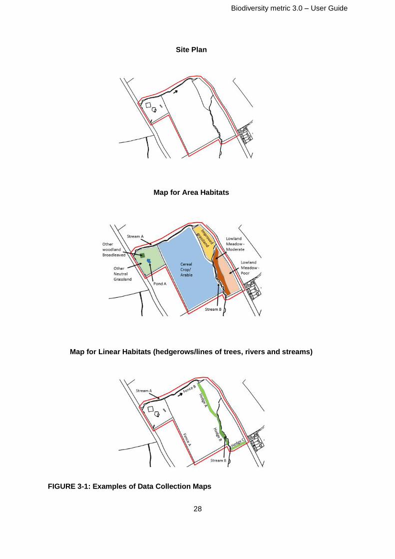
Step 2: Site visit – identifying and mapping habitats
a. An initial site walkover will help identify how the site might best be split into habitat
parcels and surveyed most effectively. During the walkover, consider different land
uses across the site and identify any areas of higher biodiversity interest (i.e. areas of
Priority Habitat or features with potential to support protected species) which may
require bespoke survey effort (see Figure 3-1).
b. Where practical, it is advisable to use digital mapping in the field, as this will typically
allow more accurate recording of boundaries and make the process of revising maps
easier. Using an appropriately scaled, geo-referenced plan or aerial image, the site
should then be divided into habitat parcels (contiguous areas of habitats having the
same type and condition) as appropriate and hedgerow/watercourse lengths
(contiguous areas of hedgerow/watercourse having the same type and condition).
24 Training details can be found at https://modularriversurvey.org/river-condition
Biodiversity metric 3.0 – User Guide
22
c. For rivers and streams, the number of MoRPh (Modular River Physical) surveys25,26
to complete will differ depending on the site and the character of the river. The string
of MoRPh 5s should capture a minimum 20% length of the river within the on-site
area; this will enable changes in riverine condition to be captured. Surveyors should
choose the location of their survey sites where noticeable changes in river condition
occur e.g. areas of high riverine/riparian quality, areas of physical modification, areas
where restoration could occur, areas of potential impact. A walkover of the site before
selecting the survey sites is essential.
d. When a ditch is present alongside a hedgerow it should only be recorded once in the
metric. Ditches should EITHER be recorded as:
• a hedgerow or line of trees associated with a bank or ditch OR
• a ditch in the rivers and streams metric (See Box 3-1 below).
BOX 3-1: Hedges and lines of trees associated with ditches
For these purposes a ditch is defined as follows:
For inclusion in the Hedgerows metric, a ditch is ‘a linear depression running adjacent
to a hedge or Line of trees (<2m from the hedgerow centre) which may or may not
hold water for part of the year.’
For inclusion in the rivers and streams Metric, a ditch is an ‘Artificially created, linear
water-conveyancing features that are less than 5 m wide and likely to retain water for
more than 4 months of the year. Their hydraulic function is primarily for land drainage,
and although partially or fully connected to a river system, they would not have been
present without human intervention’.
When a ditch meets the definition for the rivers and streams metric it should be
accounted for separately in the rivers and streams metric and, if it occurs adjacent to a
hedge or line of trees, the hedgerow type should be determined and recorded
separately without recognition of the ditch.
If surveying in the winter, the vegetation should indicate whether the ditch is of an
ephemeral nature or not.
e. Hedgerows are mapped as linear features. Area habitats adjacent to hedgerows
should be mapped to the centre line of the hedgerow (defined on OS maps by a
black line). This will result in a slight overestimation of the area and resulting
biodiversity units generated by habitats adjacent to hedgerows.
25 SHUKER, L.J., GURNELL, A.M., WHARTON, G., GURNELL, D.J., ENGLAND, J., FINN LEEMING, B. &
BEACH, E., 2017. MoRPh: a citizen science tool for monitoring and appraising physical habitat changes in rivers.
Water and Environment Journal, 31(3): 418-424.
26 GURNELL, A.M., ENGLAND, J., SHUKER, L., WHARTON, G. (in review). The contribution of citizen science
volunteers to river monitoring and management: International and national perspectives and the example of the
MoRPh survey.
Biodiversity metric 3.0 – User Guide
23
f. Hedgerows bounding green lanes and double hedgerows should be recorded as two
hedgerows rather than a single hedge. This distinction recognises that double
hedges are known to be particularly important for wildlife27,28.
g. Whilst there is no firm minimum or maximum parcel size, it is recommended that a
proportionate approach is taken to avoid the recording of habitat types that cover a
total area of less than one square meter (0.0001 ha), or recording extremely large
areas that are likely to vary in their condition as one habitat parcel.
h. Habitats should be classified using either the UK Habitat Classification System29,
European Nature Information System (EUNIS)30, Water Framework Directive (WFD)
Lakes typologies31 (see Box 3-2) or the hedgerows and lines of trees key in Box 8-2.
A small number of habitats have definitions specific to biodiversity metric 3.0. This
means that habitats are classified in a way which is widely recognised and that can
be directly input into the biodiversity metric 3.0 calculation tool. All habitats used in
biodiversity metric 3.0 and their definition source are listed in Table TS2-1.
i. Unique reference numbers should be assigned to each habitat parcel, hedgerow, line
of trees or watercourse and any maps generated should clearly display the unique
reference of each parcel or linear feature.
j. Any survey limitations (e.g. access constraints or seasonal constraints) should be
noted at this point.
27 WALKER, M.P., DOVER, J.W., HINSLEY, S.A. & SPARKS, TH. 2005. Birds and green lanes: Breeding season bird abundance, territories and species richness. Biological Conservation, 126: 540–547.
28 WALKER, M.P., DOVER, J.W., SPARKS, T.H. & HINSLEY, S.A. 2006. Hedges and green lanes:
vegetation composition and structure. Biodiversity and Conservation, 15:2595–2610
29 UK Habitat Classification: http://ukhab.org
30 European Nature Information System
31 http://wfduk.org/sites/default/files/Media/Characterisation of the water environment/Lakes
typology_Final_010604.pdf
Biodiversity metric 3.0 – User Guide
24
Box 3-2: The UK Habitat Classification (UKHab)
The terrestrial area habitats in Biodiversity metric 3.0 are largely based on the UK Habitat
Classification system, a free-to-use (open access), unified and comprehensive approach
to classifying habitats that is fully compatible with other major existing classifications. It is
designed to be suitable for digital or manual use in habitat metrics, impact assessment
and sharing data between organisations.
The UK Habitat Classification system was chosen for use in the metric as it translates
easily into Priority Habitat types and Habitats Directive Annex 1 types; has scope to
incorporate assessments of condition, origin or management regime; and is compatible
with digital mapping systems.
The habitat list within biodiversity metric 3.0 includes those derived from the UK Habitat
Classification system, but also EUNIS, Water Framework Directive lakes typologies and
Annex 1 habitat types. Additionally, some UKHab types have been omitted from the metric
because they are better recorded as the actual habitat type presented on the site (e.g. a
‘railway corridor’ is better split into its individual artificial unsealed surface, grassland &
scrub types).
If habitats have been classified using JNCC Phase 1 Habitat Survey typologies, the
resulting habitat types can be translated into UKHab for use in the biodiversity metric. A
translation table between Phase 1 and UKHab types is provided within the biodiversity
metric 3.0. This translation table can be found via the ‘Technical Data’ button in the
calculation tool.
Step 3: Site visit – assessing habitat condition
a. All habitat parcels, hedgerows and watercourses must be assigned a habitat
condition score: this is a measure of the habitat’s quality. Habitat condition can only
be assessed after a land parcel, hedgerow or watercourse has been assigned a
habitat type (see Table 3-1).
b. The full methodology for assessing habitat condition is set out within Part 1a of the
Technical Supplement. The condition assessment criteria for Hedgerows and Lines
of trees are set out within Part 1b of the Technical Supplement.
c. During a condition assessment, a habitat parcel, hedgerow length or watercourse
may be deemed to contain areas of differing condition. If this is the case, the habitat
parcel, hedgerow length or stretch of watercourse must be split accordingly to ensure
each parcel represents habitat of the same type and condition.
d. On completion of condition assessments, all habitat parcels should be assigned one
of three condition categories: Good, Moderate or Poor. The metric tool does allow for
intermediate categories (Fairly Good and Fairly Poor) if it is not possible to
distinguish between two main condition categories. Justification for use of either
intermediate condition category should be noted during the site visit and recorded
within the ‘assessor comments’ column of the metric tool.
e. If any habitats in the site have recently been destroyed or degraded and it is deemed
appropriate to use pre-degradation habitats as the site’s baseline, a precautionary
approach should be taken to recording the habitat previously present. This approach
Biodiversity metric 3.0 – User Guide
25
should make use of any evidence remaining on site, or from the desk-based
assessment (see 3.9 Step 1, c), and assume high distinctiveness and good condition
for lost or degraded habitats in the absence of evidence to the contrary. The
approach should be agreed with the relevant decision maker for the site or project
and should be justified in the ‘assessor comments’ section of the metric calculator.
For example, if an area identified in the desk-based study is recorded as scrub
habitat in credible recent mapping or aerial photography and upon arrival the site is
now found to be cleared of all vegetation, it should normally be recorded as ‘mixed
scrub’ in ‘good’ condition.
f. Any additional survey limitations (e.g. access constraints or seasonal constraints)
should also be noted at this point.
Step 4: Site visit – opportunities for on-site habitat creation & enhancement
a. As well as collecting data on existing habitats, hedgerows, and watercourses it is
also advisable to use any site visits to identify opportunities for enhancement of
existing habitat or creation of new habitat. This may help inform development design,
ecological mitigation, and ongoing habitat management and maintenance activities.
b. The River Condition Assessment Information System can be used to support
scenario modelling of proposed changes to inform potential mitigation options. To
forecast predicted post-intervention condition scores, re-run the river condition
assessment with planned river restoration interventions and anticipated channel
responses. Alternatively, look at the values of the 32 positive and negative ‘Condition
Indicator’ scores to help understand which features can be changed to achieve net
gain and then adjust the scores to take account of the impacts of the proposed
interventions.
Step 5: After site visit – assigning strategic significance
a. All habitat parcels (both baseline and post-intervention) must be assigned a strategic
significance score. Recognising strategic significance gives extra value to habitats
that are located in optimal locations, or are of a type, that meet local objectives for
biodiversity.
b. The approach taken to determine strategic significance is described in Sections 5.15
and 8.52. For development projects, the relevant local plans and strategies will be
determined by the relevant local planning authority.
c. A score should be assigned to each habitat parcel according to the habitat type and
what is identified as a priority in a particular area. The options for scoring each
habitat parcel are:
• High - Within area formally identified in local strategy, plan or policy
• Medium - Location ecologically desirable but not identified in a local strategy,
plan or policy
• Low - Not identified in a local strategy, plan or policy OR No strategy or plan
is in place in the area
Biodiversity metric 3.0 – User Guide
26
Step 6: After site visit – preparing data for use in biodiversity metric calculator tool
a. Baseline data should be assigned a habitat category from Table TS2-1 on collection
or, if recorded using an alternative habitat typology, converted to one of these for
entry into the metric calculation tool (see Box 3-2).
b. On-site post-intervention habitat data may be created using landscape habitat
typologies but must also be converted to a habitat type in Table TS2-1 for entry into
the metric calculation tool. This conversion should be based on proposed planting
plans and collaboration with the landscape architect is recommended at this stage.
c. For both baseline and post-intervention data, ensure each habitat parcel, hedgerow
or watercourse has been assigned a unique ID (this can be the row number in the
metric calculation tool). Any maps generated to support the calculation should clearly
display the unique ID of each parcel.
d. For both baseline and post-intervention data, ensure the total area being assessed is
equal to the sum of all habitat polygons mapped. Include justification in the surveyor
comments section if this is not the case (e.g. if the site contains a 5m wide river
channel – see h. below). Ensure the sum of baseline & post-intervention habitat
parcels are equal, or that any discrepancies are explained. Any overlaps, duplicates
or gaps in digital mapping must be resolved before entering data into the metric
calculator tool.
e. Where there is an overlap between the developed area (e.g. a building) and an urban
habitat (for example a green roof) then only the surface (i.e. open to the sky) habitat
should be recorded. In these scenarios the area of developed land/sealed surface
should be reduced by the area of the green roof.
f. In the rare circumstances where there is overlapping habitat for example a cantilever
green roof over a vegetated garden both can be recorded, and a justification made
regarding the discrepancy in area. As GIS systems only record in 2D, the underlying
vegetated garden would need to be entered manually (with appropriate justification) if
using the QGIS data import template.
g. If you intend to use the QGIS data import template, you will also need to follow the
accompanying guidance32 relating to data format.
h. The area occupied by rivers and streams habitats greater than 5 metres wide can be
recorded as areas as well as lengths. The length will be input into the metric in order
to calculate river biodiversity units. The area the watercourse occupies should be
noted and excluded from the area biodiversity unit calculation (pre-intervention and
post-intervention). This means that, in some circumstances, the sum of the area
habitats recorded in the metric will be less than the total site area.
32 Biodiversity Metric 3.0 QGIS template and GIS import tool guidance – Beta test
Biodiversity metric 3.0 – User Guide
27
i. Newly excavated river channels will result in a loss in area habitats. Record the loss
of area habitat type in the pre-intervention section of the biodiversity metric
calculation tool. Similarly, the previous river channels (if a new one has been
excavated) may be used to create new areas of habitat such as reedbed or wet
woodland.
j. When recording a newly created river channel, the details should be entered as
creation or enhancement as appropriate (see Table 8-9).
k. When a river restoration scheme restores a channel line, the length of the final river
may be longer than the original river baseline. This may be due to increasing the
number of meander bends or by including a by-pass channel. This can be accounted
for in biodiversity metric 3.0 by entering this final restored length into the ‘length
enhanced’ column (column U) of the baseline tab. This enhanced length is then
automatically applied in the river enhancement tab.
l. When a scheme restores several channels, for example in a braided system, include
the final length of restored river channel in the length enhanced column.
Biodiversity metric 3.0 – User Guide
28
Site Plan
Map for Area Habitats
Map for Linear Habitats (hedgerows/lines of trees, rivers and streams)
FIGURE 3-1: Examples of Data Collection Maps
Biodiversity metric 3.0 – User Guide
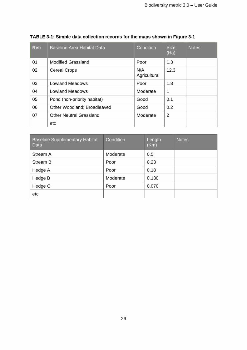
29
TABLE 3-1: Simple data collection records for the maps shown in Figure 3-1
Ref: Baseline Area Habitat Data Condition Size (Ha)
Notes
01 Modified Grassland Poor 1.3
02 Cereal Crops N/A Agricultural
12.3
03 Lowland Meadows Poor 1.8
04 Lowland Meadows Moderate 1
05 Pond (non-priority habitat) Good 0.1
06 Other Woodland; Broadleaved Good 0.2
07 Other Neutral Grassland Moderate 2
etc
Baseline Supplementary Habitat Data
Condition Length (Km)
Notes
Stream A Moderate 0.5
Stream B Poor 0.23
Hedge A Poor 0.18
Hedge B Moderate 0.130
Hedge C Poor 0.070
etc
Biodiversity metric 3.0 – User Guide
30
4: How to use the Calculation Tool
4.1 The biodiversity metric 3.0 guidance is accompanied by a calculation tool. A short
guide explaining how to use the calculation tool is also available.
4.2 To use the calculation tool, users will need access to data which covers:
• Habitat types
• Area/length of habitats
• Habitat condition
• Strategic significance of each habitat
• Area to be retained/enhanced
• Whether bespoke compensation has been agreed (when applicable)
• Timing of habitat creation (i.e. in advance of habitat loss or delayed)
4.3 The biodiversity metric 3.0 calculation tool is pre-populated with much of the key data
that is needed for the calculation. There are separate data entry buttons for pre- and
post-intervention for on-site and off-site data (see Figure 4-3) and. It provides
headline results as well as detailed results, outputs and graphics.
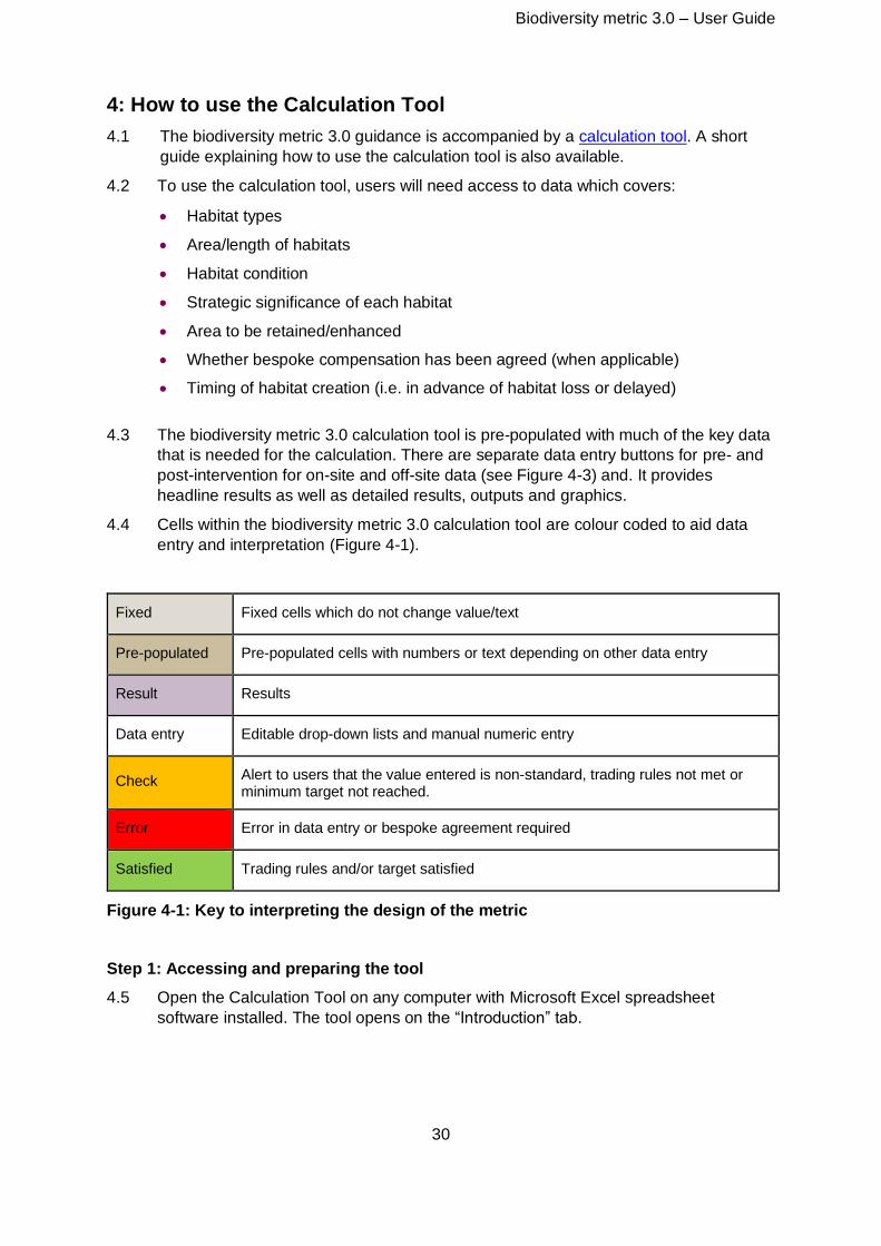
4.4 Cells within the biodiversity metric 3.0 calculation tool are colour coded to aid data
entry and interpretation (Figure 4-1).
Fixed Fixed cells which do not change value/text
Pre-populated Pre-populated cells with numbers or text depending on other data entry
Result Results
Data entry Editable drop-down lists and manual numeric entry
Check Alert to users that the value entered is non-standard, trading rules not met or minimum target not reached.
Error Error in data entry or bespoke agreement required
Satisfied Trading rules and/or target satisfied
Figure 4-1: Key to interpreting the design of the metric
Step 1: Accessing and preparing the tool
4.5 Open the Calculation Tool on any computer with Microsoft Excel spreadsheet
software installed. The tool opens on the “Introduction” tab.
Biodiversity metric 3.0 – User Guide
31
4.6 The metric works best with macros and content enabled33, and macros must be
enabled upon opening the metric to use the navigation buttons.
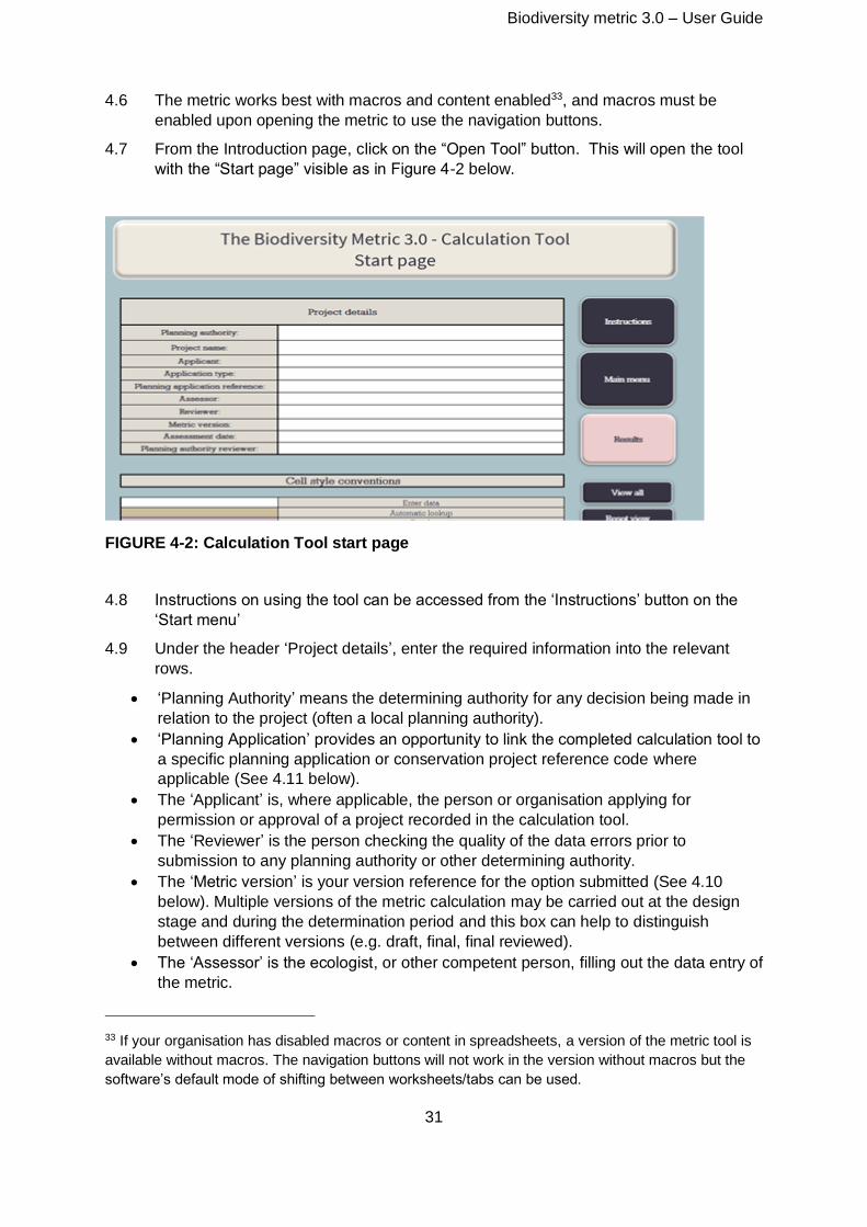
4.7 From the Introduction page, click on the “Open Tool” button. This will open the tool
with the “Start page” visible as in Figure 4-2 below.
FIGURE 4-2: Calculation Tool start page
4.8 Instructions on using the tool can be accessed from the ‘Instructions’ button on the
‘Start menu’
4.9 Under the header ‘Project details’, enter the required information into the relevant
rows.
• ‘Planning Authority’ means the determining authority for any decision being made in
relation to the project (often a local planning authority).
• ‘Planning Application’ provides an opportunity to link the completed calculation tool to
a specific planning application or conservation project reference code where
applicable (See 4.11 below).
• The ‘Applicant’ is, where applicable, the person or organisation applying for
permission or approval of a project recorded in the calculation tool.
• The ‘Reviewer’ is the person checking the quality of the data errors prior to
submission to any planning authority or other determining authority.
• The ‘Metric version’ is your version reference for the option submitted (See 4.10
below). Multiple versions of the metric calculation may be carried out at the design
stage and during the determination period and this box can help to distinguish
between different versions (e.g. draft, final, final reviewed).
• The ‘Assessor’ is the ecologist, or other competent person, filling out the data entry of
the metric.
33 If your organisation has disabled macros or content in spreadsheets, a version of the metric tool is
available without macros. The navigation buttons will not work in the version without macros but the
software’s default mode of shifting between worksheets/tabs can be used.
Biodiversity metric 3.0 – User Guide
32
4.10 Complete all relevant sections of the start page, including inserting illustrative design
images of both the baseline and post development scenarios if these are available or
required for the project.
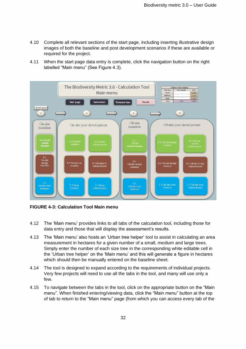
4.11 When the start page data entry is complete, click the navigation button on the right
labelled “Main menu” (See Figure 4.3).
FIGURE 4-3: Calculation Tool Main menu
4.12 The ‘Main menu’ provides links to all tabs of the calculation tool, including those for
data entry and those that will display the assessment’s results.
4.13 The ‘Main menu’ also hosts an ‘Urban tree helper’ tool to assist in calculating an area
measurement in hectares for a given number of a small, medium and large trees.
Simply enter the number of each size tree in the corresponding white editable cell in
the ‘Urban tree helper’ on the ‘Main menu’ and this will generate a figure in hectares
which should then be manually entered on the baseline sheet.
4.14 The tool is designed to expand according to the requirements of individual projects.
Very few projects will need to use all the tabs in the tool, and many will use only a
few.
4.15 To navigate between the tabs in the tool, click on the appropriate button on the “Main
menu”. When finished entering/viewing data, click the “Main menu” button at the top
of tab to return to the “Main menu” page (from which you can access every tab of the
Biodiversity metric 3.0 – User Guide
33
tool). If you are using a macro-free version use the tabs shown at the bottom or the
window.
Step 2: Baseline (pre-intervention) data entry
Entering baseline data
4.16 The baseline provides a proxy measure for the quality, quantity and type of habitat
within the site boundary prior to an intervention (e.g. a development or conservation
project).
4.17 The information you will need to enter to complete your baseline assessment will
depend on the type of habitats you have on your site, and whether you are including
any off-site habitat (also referred to as offsets).
4.18 The ‘On-site baseline’ tabs should always be completed for all present habitat types.
4.19 If the metric is being used to calculate the biodiversity units of an off-site intervention
(e.g. an offset for a development project) ‘Off-site baseline’ tabs should also be
completed for all habitat types present within the off-site boundary.
4.20 Providers of off-site interventions (e.g. a land manager providing an offset for a
development elsewhere) should use the off-site baseline tab and start at step 4.
4.21 Once the relevant baseline data entry tab is open, the “Condense/show columns”
buttons, and equivalents for rows, can be used at any time.
Completing the baseline calculation
4.22 This section of the tool allows you to describe the habitats as they are before the
intervention (e.g. development or conservation project) takes place.
4.23 The A-1 On-Site Habitat Baseline tab allows you to enter data for the area habitats
that are already present on your site (See Figure 4-3). You will need to select or
enter information about the following:
• Broad habitat
• Habitat type
• Habitat area
• Habitat condition
• Strategic significance
• Area to be retained/enhanced
• Whether bespoke compensation has been agreed (when applicable)
• Comments (optional)
Top Tip: Prepare your data before completing the metric calculation tool. Think about
how the individual parcels within the site will change after the intervention and which
habitats will be lost, retained and enhanced.
Biodiversity metric 3.0 – User Guide
34
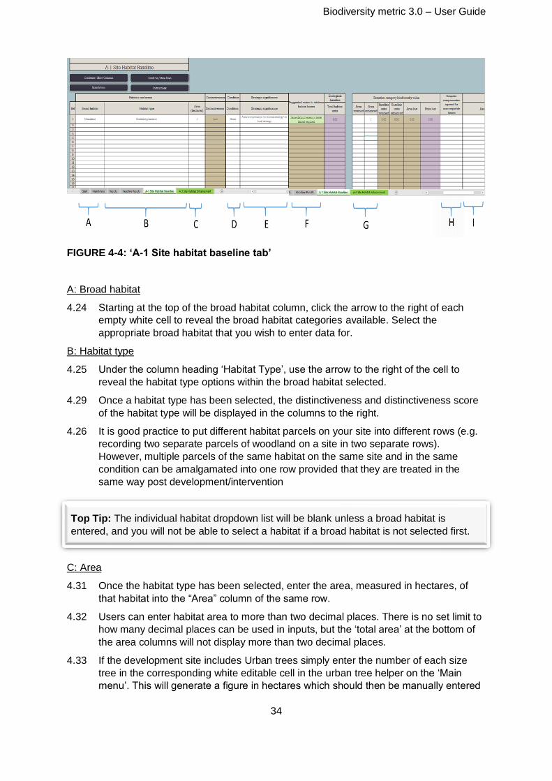
FIGURE 4-4: ‘A-1 Site habitat baseline tab’
A: Broad habitat
4.24 Starting at the top of the broad habitat column, click the arrow to the right of each
empty white cell to reveal the broad habitat categories available. Select the
appropriate broad habitat that you wish to enter data for.
B: Habitat type
4.25 Under the column heading ‘Habitat Type’, use the arrow to the right of the cell to
reveal the habitat type options within the broad habitat selected.
4.29 Once a habitat type has been selected, the distinctiveness and distinctiveness score
of the habitat type will be displayed in the columns to the right.
4.26 It is good practice to put different habitat parcels on your site into different rows (e.g.
recording two separate parcels of woodland on a site in two separate rows).
However, multiple parcels of the same habitat on the same site and in the same
condition can be amalgamated into one row provided that they are treated in the
same way post development/intervention
C: Area
4.31 Once the habitat type has been selected, enter the area, measured in hectares, of
that habitat into the “Area” column of the same row.
4.32 Users can enter habitat area to more than two decimal places. There is no set limit to
how many decimal places can be used in inputs, but the ‘total area’ at the bottom of
the area columns will not display more than two decimal places.
4.33 If the development site includes Urban trees simply enter the number of each size
tree in the corresponding white editable cell in the urban tree helper on the ‘Main
menu’. This will generate a figure in hectares which should then be manually entered
Top Tip: The individual habitat dropdown list will be blank unless a broad habitat is
entered, and you will not be able to select a habitat if a broad habitat is not selected first.
Biodiversity metric 3.0 – User Guide
35
the baseline sheet in the same way as other habitats in order to calculate the
biodiversity units. Note: This will need to be repeated for trees of different condition
which will need to be entered on separate rows in the metric.
D: Condition
4.34 Using the relevant information (see 3.9, Step 3), select the habitat condition for each
row of habitat using the dropdown list in the “Condition” column. The tool will then
automatically apply the corresponding condition score.
4.35 The choice in the condition dropdown list is dependent on the type of habitat entered.
The list of condition options will therefore not be revealed until a habitat type is
selected
4.36 If two parts of the same habitat are of different condition, they should be split across
two rows and recorded as two separate parcels.
E: Strategic significance
4.37 Under the column heading ‘Strategic significance”, use the arrow to the right of the
cell to reveal the options.
4.38 Select the option for each habitat that best corresponds to information set out in local
plans or policies for that particular habitat and its location. The tool will then
automatically apply the corresponding strategic significance score.
4.39 Strategic significance should be considered separately for each individual habitat
entry in the metric and not on a site wide basis. Habitat not specified in some form of
strategy, map or plan for that area should not be considered strategically significant.
4.40 ‘Within an area formally identified in a local strategy’ should only be selected for those
specific habitats identified as being geographically important within relevant local
strategies. For example if the development site or offset site contains a mixture of
habitats and is within an area identified as strategically important for Lowland
calcareous grassland it is only the Lowland calcareous grassland that should be
recorded as ‘Within an area formally identified in a local strategy’.
4.41 When a local strategy identifies an area as ecologically significant generically, such
as a Local Site or strategic ecological corridor, all habitats occurring within that area
should be identified as ‘Within an area formally identified in a local strategy’.
4.42 When no such strategy exists, or the area in question does not fall within the local
strategy, professional judgement may be used to determine whether a habitat should
be identified as ‘Location ecologically desirable but not in a local strategy’ and
justification provided. See 5.20 for guidance.
Top Tip: If a score for condition is shown as “Not possible”, it means that the habitat type
is not compatible with the selected condition state. This can occur if the habitat type has
been changed to one that is not compatible after assigning a condition. To remedy this,
simply change your condition input and the error message will disappear.
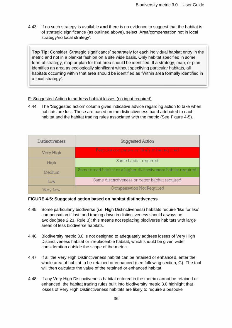
Biodiversity metric 3.0 – User Guide
36
4.43 If no such strategy is available and there is no evidence to suggest that the habitat is
of strategic significance (as outlined above), select ’Area/compensation not in local
strategy/no local strategy’.
F: Suggested Action to address habitat losses (no input required)
4.44 The ‘Suggested action’ column gives indicative advice regarding action to take when
habitats are lost. These are based on the distinctiveness band attributed to each
habitat and the habitat trading rules associated with the metric (See Figure 4-5).
Distinctiveness Suggested Action
Very High Bespoke compensation likely to be required
High Same habitat required
Medium Same broad habitat or a higher distinctiveness habitat required
Low Same distinctiveness or better habitat required
Very Low Compensation Not Required
FIGURE 4-5: Suggested action based on habitat distinctiveness
4.45 Some particularly biodiverse (i.e. High Distinctiveness) habitats require ‘like for like’
compensation if lost, and trading down in distinctiveness should always be
avoided(see 2.21, Rule 3); this means not replacing biodiverse habitats with large
areas of less biodiverse habitats.
4.46 Biodiversity metric 3.0 is not designed to adequately address losses of Very High
Distinctiveness habitat or irreplaceable habitat, which should be given wider
consideration outside the scope of the metric.
4.47 If all the Very High Distinctiveness habitat can be retained or enhanced, enter the
whole area of habitat to be retained or enhanced (see following section, G). The tool
will then calculate the value of the retained or enhanced habitat.
4.48 If any Very High Distinctiveness habitat entered in the metric cannot be retained or
enhanced, the habitat trading rules built into biodiversity metric 3.0 highlight that
losses of Very High Distinctiveness habitats are likely to require a bespoke
Top Tip: Consider ‘Strategic significance’ separately for each individual habitat entry in the
metric and not in a blanket fashion on a site wide basis. Only habitat specified in some
form of strategy, map or plan for that area should be identified. If a strategy, map, or plan
identifies an area as ecologically significant without specifying particular habitats, all
habitats occurring within that area should be identified as ‘Within area formally identified in
a local strategy’.
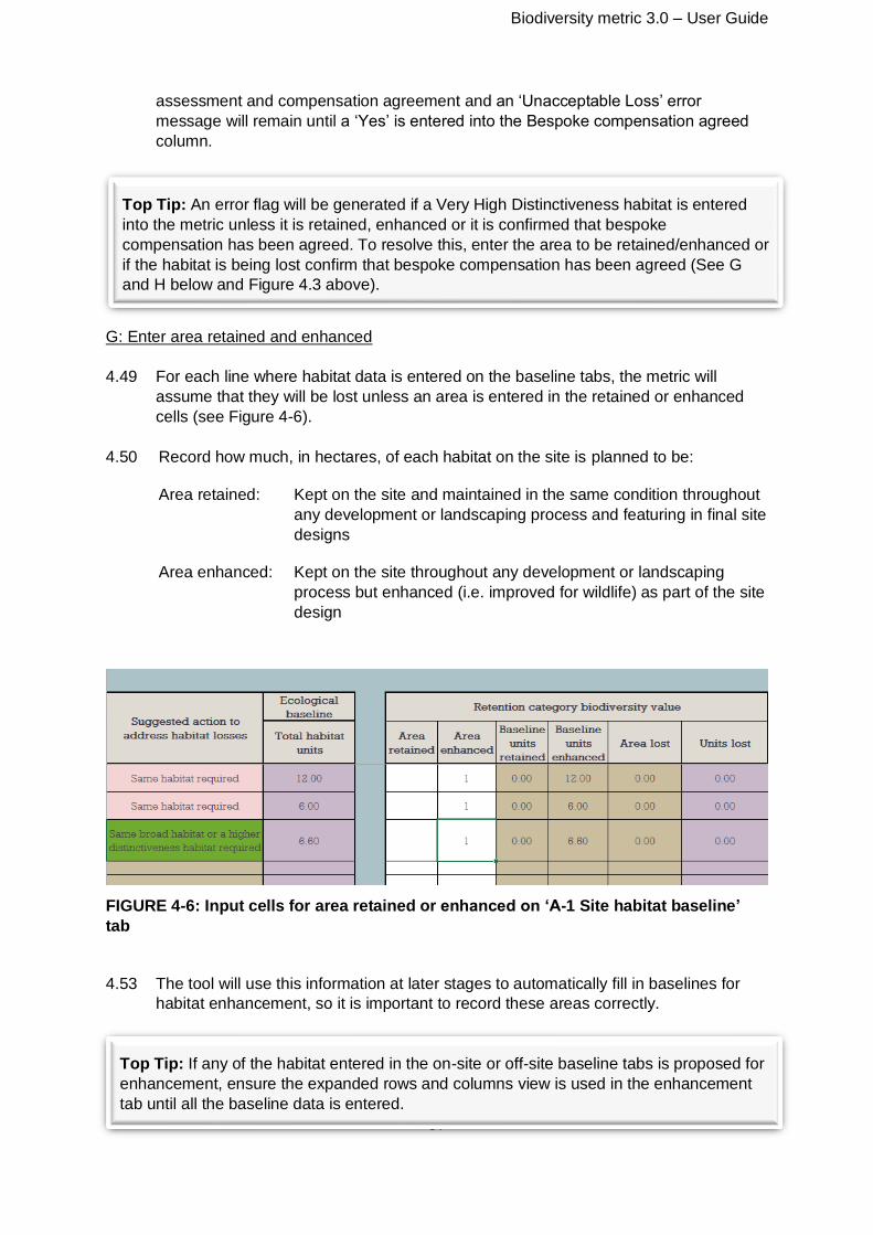
Biodiversity metric 3.0 – User Guide
37
assessment and compensation agreement and an ‘Unacceptable Loss’ error
message will remain until a ‘Yes’ is entered into the Bespoke compensation agreed
column.
G: Enter area retained and enhanced
4.49 For each line where habitat data is entered on the baseline tabs, the metric will
assume that they will be lost unless an area is entered in the retained or enhanced
cells (see Figure 4-6).
4.50 Record how much, in hectares, of each habitat on the site is planned to be:
Area retained: Kept on the site and maintained in the same condition throughout
any development or landscaping process and featuring in final site
designs
Area enhanced: Kept on the site throughout any development or landscaping
process but enhanced (i.e. improved for wildlife) as part of the site
design
FIGURE 4-6: Input cells for area retained or enhanced on ‘A-1 Site habitat baseline’
tab
4.53 The tool will use this information at later stages to automatically fill in baselines for
habitat enhancement, so it is important to record these areas correctly.
Top Tip: An error flag will be generated if a Very High Distinctiveness habitat is entered
into the metric unless it is retained, enhanced or it is confirmed that bespoke
compensation has been agreed. To resolve this, enter the area to be retained/enhanced or
if the habitat is being lost confirm that bespoke compensation has been agreed (See G
and H below and Figure 4.3 above).
Top Tip: If any of the habitat entered in the on-site or off-site baseline tabs is proposed for
enhancement, ensure the expanded rows and columns view is used in the enhancement
tab until all the baseline data is entered.
Biodiversity metric 3.0 – User Guide
38
H: Bespoke Compensation Agreed (only applicable to Very High Distinctiveness habitat)
4.54 Unless all Very High Distinctiveness habitats can be retained or enhanced, bespoke
compensation (or confirmation that it is not required) should be agreed with the
relevant decision maker (e.g. a planning authority). Once this has been agreed, select
‘Yes’ on the dropdown list in the ‘Bespoke compensation agreed’ column.
4.55 See 2.27 before applying the metric calculation tool to any site that includes
irreplaceable habitat.
I: Assessor and Local Authority Reviewer Comments
4.56 At the end (right) of each row there is a pair of comment boxes where optional text
can be added. This provides an opportunity for assessors and reviewers to make any
comments relating to a specific habitat parcel. It can be left blank if it is not needed.
Hedgerow, lines of trees and rivers and streams - baselines
4.57 If the site does not contain these habitats, proceed to Step 3. If the site contains
hedgerows and/or lines of trees, or rivers, streams, canals or ditches, you should
complete the relevant tabs of the metric calculation tool for these habitats. For lines of
trees use the ‘hedge baseline’ buttons and tabs. Use the main menu to navigate to
tabs B-1 and C-1.
4.58 Enter the relevant data for these habitats, as you would for area (non-linear) habitats.
However, habitat extent should be recorded as length in kilometres of the habitat
feature rather than the area in hectares.
Step 3: Post-intervention data entry
Navigating the post-intervention data entry tabs
4.59 Use the ‘Main menu’ in the tool to determine which post-intervention data entry tabs
you will need to complete. The tabs you will need to complete will depend on the type
of habitats you include in your designs, and whether you are creating habitats or
enhancing habitats.
4.60 In most cases, the first post-intervention data entry tab to complete will be “A-2 Site
Habitat Creation” found within the “On-site post development” section.
4.61 After entering data for the habitats that will be created return to the ‘Main menu’ and
select the “A-3 Site Habitat enhancement” also found within the “On-site post
development” section.
Top Tip: Use this section to record any additional justifications for the assessment of
habitat type, condition or location if needed.
Biodiversity metric 3.0 – User Guide
39
4.62 This section of the tool allows you to describe the habitats as they will be after the
planned development or other intervention takes place and generate a biodiversity
unit value.
On-site habitat creation
4.63 These tabs allow you to enter the data for the habitats which you plan to create in the
same way as is done for the baseline assessment. The tool will then automatically
apply the appropriate difficulty and temporal risk multipliers for each created habitat
and calculate the number of biodiversity units generated.
4.64 You will need to select or enter information relating to the proposed:
• Broad habitat
• Habitat type
• Habitat area
• Habitat condition
• Strategic significance assessment
• Whether habitat creation has been undertaken in advance or will be delayed,
relative to any losses of on-site habitats
• Comments (optional)
4.65 If a score for condition is shown as “Not possible” see Step 1 (D) above.
4.66 At the far right of each row there is a comments box which provides an opportunity for
assessors and reviewers to make any observations or comments.
4.67 The Metric cross checks for discrepancies between the baseline and post
development site areas. An error flag is triggered if the total areas for baseline post-
intervention habitats do not match. A tolerance of 0.01 hectare has been built into the
tool to avoid unnecessarily triggering an error message due to rounding errors and
mapping inaccuracies.
New habitat created in advance of loss
4.68 Biodiversity metric 3.0 rewards habitat creation in advance by reducing the difficulty
and temporal risk multipliers applied. This reflects the lower delivery risk; there is less
risk of failure when a habitat is already making progress towards its target condition.
Top Tip: Use the comments box to provide a brief rationale for an action or some
additional context. For example, to justify why a particular condition was chosen.
Top Tip: If an error flag is triggered there is a discrepancy bigger than 0.01 ha that needs
to be addressed.
Check the area of habitat entered for pre and post development to identify and correct any
errors identified. Use the comments box for the relevant habitat to provide a brief rationale
for an action or some additional context if there is a good reason why there is a
discrepancy.
Biodiversity metric 3.0 – User Guide
40
4.69 If work to create a habitat parcel has been undertaken in advance of any impact it is
compensating for, the number of full years between these dates should be entered
the habitat created in advance column for that parcel’s row. The tool then
automatically reduces the timescale to reach target condition by this number of years
and adjusts the temporal multiplier.
4.70 Once a habitat has been established for enough time to reach or exceed the
predetermined timescale for poor condition for that specific habitat, the metric tool will
apply the predetermined difficulty risk associated with enhancing rather than creating
that habitat.
4.71 Once a habitat has been established for long enough to meet the predetermined
timescale to reach the desired condition the temporal and risk multipliers are
neutralised.
4.72 Evidence of the advance habitat creation work is likely to be required by the relevant
determining authority/decision maker.
4.73 If no habitat creation works will be undertaken in advance, the cell can be left blank or
‘0’ can be selected.
Delay in starting habitat creation
4.74 This function should be applied if there will be a significant delay in the creation of a
habitat type relative to any losses of on-site habitats. For example, to account for
delays due to phased developments and developments that temporarily require parts
of the development site for construction purposes (which are not reinstated to their
former condition within 2 years. See 5.55 regarding losses which may be considered
temporary).
4.75 Enter the number of full years that the creation will be delayed into the ‘Delay in
starting Habitat Creation’ column.
4.76 The number of years entered here will be added to the pre-populated time to target
condition and increase the effect of the risk multiplier accordingly.
4.77 If the creation of habitats will not be delayed, the cell can be left blank or a ‘0’ can be
selected.
On-site habitat enhancement
4.78 These tabs allow you to enter the data for the habitats which you plan to enhance in
the same way as is done for the baseline assessment. The tool will then automatically
apply the appropriate difficulty and temporal risk multipliers for each habitat and
calculate the number of biodiversity units generated.
4.79 When you enter the area of habitat being enhanced into the “Area enhanced” column
of the on-site or off-site baseline tabs, the tool will automatically list the habitats you
Top Tip: If a value greater than 0 is entered in both the advance creation and the delayed
creation cells for the same row the metric will generate an error and will not proceed with
the calculation. Select either the advance creation or the delayed creation but not both.
Biodiversity metric 3.0 – User Guide
41
plan to enhance on the corresponding habitat enhancement tab, using the data you
first put into the baseline tabs (See Figure 4-4).
4.80 You will need to select or manually enter data for the proposed:
• Broad habitat
• Habitat type (if enhancing to a higher distinctiveness habitat type within the same
broad habitat)
• Habitat condition
• Strategic significance assessment
• Habitat enhanced in advance of development or delayed
• Comments (optional)
4.81 The existing habitat is the starting point for habitat enhancement and the tool tracks
changes in both distinctiveness and condition between the baseline and the proposed
outcome. If a trading down (See Rule 3) error occurs it will prevent the tool calculating
a value until it is resolved.
4.82 The Broad habitat and Habitat type cells are pre-populated automatically with the
habitats that were entered at the baseline, when a figure was inserted in the Area
Enhanced cell on the baseline tab.
4.83 These cells are white and optionally editable should the user wish to enhance a
habitat to a higher distinctiveness habitat within the same broad habitat.
4.84 Changing to a different broad habitat type would generally be considered as habitat
creation not enhancement (See Box 5-3). If enhancement across broad habitats is
recorded this must be ecologically justified as enhancement and the reasoning
explained in the ‘assessor comments’ cell.
Top Tip: If the baseline data is not appearing correctly in the enhancement tab, check that
you entered an area in the corresponding “Area enhanced” column of the baseline sheets
A-1 etc. (See Figure 4.4).
Top Tip: If a trading error occurs in either the distinctiveness or condition change cells in
the enhancement tab the tool will not calculate a value. To resolve the error, change the
proposed habitat or proposed condition.
Condition must stay the same or improve, even when enhancement to a higher
distinctiveness habitat is proposed, or an error will be generated.
Top Tip: If the Broad habitat and Habitat type cells are not pre-populated it may be
because you have over-ridden the pre-population function. Download a new version of
the metric or manually enter the correct habitat.
Biodiversity metric 3.0 – User Guide
42
Step 4: Off-site data entry
4.85 This tab can be used to calculate the contribution of any off-site changes towards a
project’s overall biodiversity change (loss or gain) calculation. If you need to use off-
site tabs, you will first need to enter any baseline data for the off-site location. For
example, if you were creating a woodland on an arable field away from the main (on-
site) project site, you would need to record the arable field in the off-site baseline
tabs.
4.86 To do this select the ‘Off-site baseline’ tab from the ‘Main menu’ and enter the
baseline data for off-site habitats in the same way as for the on-site habitats by
following the guidance at Step 2.
4.87 You will need to enter any data for off-site habitat creation or enhancement
separately to that for on-site habitats but using the same process. Use the Main menu
to find the appropriate off-site tabs.
4.88 For habitat creation and enhancement undertaken off-site, there is an additional
spatial risk multiplier which takes account of the proximity of the on and off-site
locations.
Step 5: Viewing and interpreting the results
4.89 From the main menu, select the ‘Results’ button located in the top right-hand side of
the page. The results are presented in three ways: Headline results; Detailed results
and Habitat trading summary.
4.90 Use the Headline results to see the overall net changes in biodiversity units and refer
to the Detailed results and Habitat trading summary to understand the see the
proposed changes in terms of habitats and areas.
Headline results tab
4.91 The Headline results tab provides a high-level summary and highlights whether
biodiversity losses or gains have been achieved across the area and linear metrics
relevant for the project.
4.92 It displays both on-site and off-site data in biodiversity units for baseline and post-
intervention states. The Headline results also provide a summary of the project-wide
change in both biodiversity unit value and percentage change.
4.93 ‘On-site net % change’ identifies the net gain or loss as a percentage of the on-site
baseline. The combined on and off-site net gain or loss is displayed under ‘Total on-
site net % change plus off-site surplus’.
4.94 When a habitat has no baseline unit value and new habitat is created, the percentage
increase is displayed as 100% net change. In these scenarios check for locally
defined unit targets which should be considered in addition to these percentage
increases.
Top Tip: Results for habitats based on an area measure are not comparable with those
based on a linear measure and therefore need to be accounted for separately.
Biodiversity metric 3.0 – User Guide
43
4.95 At the bottom of the headline results tab is a ‘Trading summary met’ box. If the
trading summary is not met, see the detailed results and trading summary tabs to
understand why.
4.96 The results for hedgerows and rivers are displayed separately from habitats based on
an area measure and should be reported on separately.
Detailed results tab
4.97 The detailed results provide a more comprehensive picture of the habitat changes.
They also display both on-site and off-site data in biodiversity unit values and
area/length.
4.98 Data for habitats based on an area measure are displayed at the at the broad habitat
level and those for hedgerows and rivers are based on hedgerow type and river type.
Habitat trading summary tab
4.99 The trading summary tab provides details of trading between habitat types and an
indication of whether the development has abided by the trading rules (See 2.21,
Rule 3).
4.100 The trading summary avoids the need to track the changes in habitat type and
condition on an individual parcel by parcel basis, which is not practical, particularly on
larger sites.
4.101 Instead the trading summary draws aggregated data from other parts of the tool and
presents the data in a way that allows assessors and reviewers to understand the
habitat changes in each distinctiveness band and determine whether or not trading
principles described in Rule 3 have been adhered to.
Error checking
4.102 The tool contains several inbuilt error messages which are designed to identify errors
in data entry. Typically, they can be resolved by checking the input data and common
causes of errors include:
• inappropriate condition ratings
• habitat areas that do not match
• aiming to create a habitat or condition type that is not considered ecologically
feasible
• Incomplete/missing data for example if an area of habitat is identified as being
enhanced in the baseline, but no data has been entered in the enhancement tab.
Top Tip: If habitat enhancement units are not included in the Headline results check all
the data in the enhancement tab has been entered correctly.
Top Tip: If a habitat is highlighted amber there are losses in that habitat type or broad
habitat group. If the trading rules are not satisfied, amber highlighted habitats identify
where the error is occurring.
Biodiversity metric 3.0 – User Guide
44
Step 6 (optional): Understanding and checking supporting data in the tool
4.103 An understanding the full data sets that drive the tool is not required for normal use,
but regular users of the tool might want to look at the underlying data to better
understand the tool’s outputs.
4.104 All the technical data and multipliers underpinning the calculation can be accessed by
clicking the ‘Technical data’ button on the main menu.
4.105 This will open the ‘Technical data’ tab which is another menu to access tabs G-1 to
G-9 of the calculation tool which provide details of the habitats within the metric and
associated technical data such as distinctiveness bands and risk multipliers.
4.106 The ‘Technical data’ tab also contains a ‘Translation tool’ ‘Translation tool’ which
enables the conversion of habitat types between Phase 1 and UKHab typologies.
Biodiversity metric 3.0 – User Guide
45
5: Detailed description of biodiversity metric 3.0
5.1 This chapter describes the components of biodiversity metric 3.0, the values used for
different multipliers, why those multipliers are used, and the assumptions and
limitations around them. It also outlines some of the factors that can be considered
when designing a project being assessed with the metric
5.2 This chapter focuses on the key components which apply to all three habitat unit
calculations in biodiversity metric 3.0 – area habitats, hedgerows and lines of trees
and rivers and streams. Chapter 6 provides further detail regarding area habitat
biodiversity unit calculations. The urban tree component is detailed in Chapter 7 and
Chapter 8 provides similar details and explanations for the linear units covering
hedgerows and lines of trees and rivers and streams.
Components of biodiversity quality
Distinctiveness
5.3 Habitat types are each assigned to a distinctiveness band. The distinctiveness of a
habitat is considered as a component of the quality of a habitat parcel. These are
based on an assessment of the distinguishing features of a habitat or linear feature,
including the consideration of species richness, rarity (at local, regional, national and
international scales), and the degree to which a habitat supports species rarely found
in other habitats.
5.4 The distinctiveness band of each habitat has been preassigned in biodiversity metric
3.0. A combination of simple rules and expert judgement have been used to assign
each habitat type to the appropriate distinctiveness band. Their derivation and
application to different habitats is explained in more detail in Part 2 of the Technical
Supplement. The distinctiveness categories and scores used for area habitats,
excluding intertidal habitats, are shown in Table 5-1.
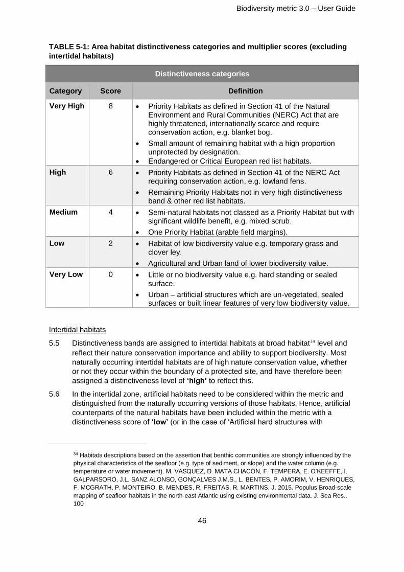
Biodiversity metric 3.0 – User Guide
46
TABLE 5-1: Area habitat distinctiveness categories and multiplier scores (excluding
intertidal habitats)
Distinctiveness categories
Category Score Definition
Very High 8 • Priority Habitats as defined in Section 41 of the Natural Environment and Rural Communities (NERC) Act that are highly threatened, internationally scarce and require conservation action, e.g. blanket bog.
• Small amount of remaining habitat with a high proportion unprotected by designation.
• Endangered or Critical European red list habitats.
High 6 • Priority Habitats as defined in Section 41 of the NERC Act requiring conservation action, e.g. lowland fens.
• Remaining Priority Habitats not in very high distinctiveness band & other red list habitats.
Medium 4 • Semi-natural habitats not classed as a Priority Habitat but with significant wildlife benefit, e.g. mixed scrub.
• One Priority Habitat (arable field margins).
Low 2 • Habitat of low biodiversity value e.g. temporary grass and clover ley.
• Agricultural and Urban land of lower biodiversity value.
Very Low 0 • Little or no biodiversity value e.g. hard standing or sealed
surface.
• Urban – artificial structures which are un-vegetated, sealed surfaces or built linear features of very low biodiversity value.
Intertidal habitats
5.5 Distinctiveness bands are assigned to intertidal habitats at broad habitat34 level and
reflect their nature conservation importance and ability to support biodiversity. Most
naturally occurring intertidal habitats are of high nature conservation value, whether
or not they occur within the boundary of a protected site, and have therefore been
assigned a distinctiveness level of ‘high’ to reflect this.
5.6 In the intertidal zone, artificial habitats need to be considered within the metric and
distinguished from the naturally occurring versions of those habitats. Hence, artificial
counterparts of the natural habitats have been included within the metric with a
distinctiveness score of ‘low’ (or in the case of ‘Artificial hard structures with
34 Habitats descriptions based on the assertion that benthic communities are strongly influenced by the
physical characteristics of the seafloor (e.g. type of sediment, or slope) and the water column (e.g.
temperature or water movement). M. VASQUEZ, D. MATA CHACÓN, F. TEMPERA, E. O’KEEFFE, I.
GALPARSORO, J.L. SANZ ALONSO, GONÇALVES J.M.S., L. BENTES, P. AMORIM, V. HENRIQUES,
F. MCGRATH, P. MONTEIRO, B. MENDES, R. FREITAS, R. MARTINS, J. 2015. Populus Broad-scale
mapping of seafloor habitats in the north-east Atlantic using existing environmental data. J. Sea Res.,
100
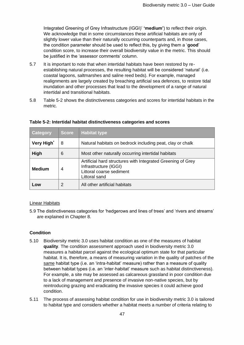
Biodiversity metric 3.0 – User Guide
47
Integrated Greening of Grey Infrastructure (IGGI)’ ‘medium’) to reflect their origin.
We acknowledge that in some circumstances these artificial habitats are only of
slightly lower value than their naturally occurring counterparts and, in those cases,
the condition parameter should be used to reflect this, by giving them a ‘good’
condition score, to increase their overall biodiversity value in the metric. This should
be justified in the ‘assessor comments’ column.
5.7 It is important to note that when intertidal habitats have been restored by re-
establishing natural processes, the resulting habitat will be considered ‘natural’ (i.e.
coastal lagoons, saltmarshes and saline reed beds). For example, managed
realignments are largely created by breaching artificial sea defences, to restore tidal
inundation and other processes that lead to the development of a range of natural
intertidal and transitional habitats.
5.8 Table 5-2 shows the distinctiveness categories and scores for intertidal habitats in the
metric.
Table 5-2: Intertidal habitat distinctiveness categories and scores
Category Score Habitat type
Very High* 8 Natural habitats on bedrock including peat, clay or chalk
High 6 Most other naturally occurring intertidal habitats
Medium 4
Artificial hard structures with Integrated Greening of Grey Infrastructure (IGGI) Littoral coarse sediment Littoral sand
Low 2 All other artificial habitats
Linear Habitats
5.9 The distinctiveness categories for ‘hedgerows and lines of trees’ and ‘rivers and streams’
are explained in Chapter 8.
Condition
5.10 Biodiversity metric 3.0 uses habitat condition as one of the measures of habitat
quality. The condition assessment approach used in biodiversity metric 3.0
measures a habitat parcel against the ecological optimum state for that particular
habitat. It is, therefore, a means of measuring variation in the quality of patches of the
same habitat type (i.e. an ‘intra-habitat’ measure) rather than a measure of quality
between habitat types (i.e. an ‘inter-habitat’ measure such as habitat distinctiveness).
For example, a site may be assessed as calcareous grassland in poor condition due
to a lack of management and presence of invasive non-native species, but by
reintroducing grazing and eradicating the invasive species it could achieve good
condition.
5.11 The process of assessing habitat condition for use in biodiversity metric 3.0 is tailored
to habitat type and considers whether a habitat meets a number of criteria relating to
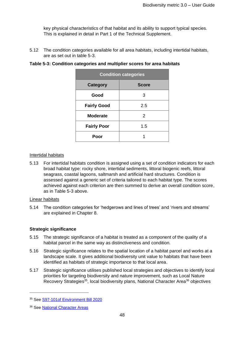
Biodiversity metric 3.0 – User Guide
48
key physical characteristics of that habitat and its ability to support typical species.
This is explained in detail in Part 1 of the Technical Supplement.
5.12 The condition categories available for all area habitats, including intertidal habitats,
are as set out in table 5-3.
Table 5-3: Condition categories and multiplier scores for area habitats
Condition categories
Category Score
Good 3
Fairly Good 2.5
Moderate 2
Fairly Poor 1.5
Poor 1
Intertidal habitats
5.13 For intertidal habitats condition is assigned using a set of condition indicators for each
broad habitat type: rocky shore, intertidal sediments, littoral biogenic reefs, littoral
seagrass, coastal lagoons, saltmarsh and artificial hard structures. Condition is
assessed against a generic set of criteria tailored to each habitat type. The scores
achieved against each criterion are then summed to derive an overall condition score,
as in Table 5-3 above.
Linear habitats
5.14 The condition categories for ‘hedgerows and lines of trees’ and ‘rivers and streams’
are explained in Chapter 8.
Strategic significance
5.15 The strategic significance of a habitat is treated as a component of the quality of a
habitat parcel in the same way as distinctiveness and condition.
5.16 Strategic significance relates to the spatial location of a habitat parcel and works at a
landscape scale. It gives additional biodiversity unit value to habitats that have been
identified as habitats of strategic importance to that local area.
5.17 Strategic significance utilises published local strategies and objectives to identify local
priorities for targeting biodiversity and nature improvement, such as Local Nature
Recovery Strategies35, local biodiversity plans, National Character Area36 objectives
35 See S97-101of Environment Bill 2020
36 See National Character Areas
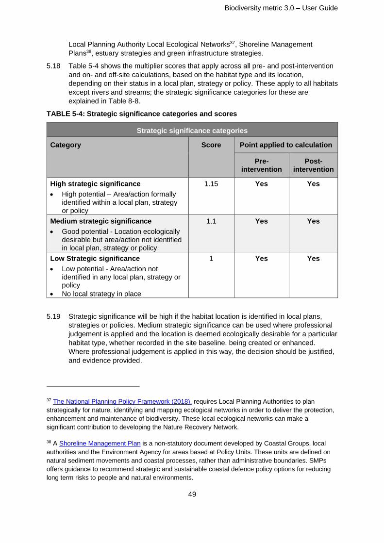
Biodiversity metric 3.0 – User Guide
49
Local Planning Authority Local Ecological Networks37, Shoreline Management
Plans38, estuary strategies and green infrastructure strategies.
5.18 Table 5-4 shows the multiplier scores that apply across all pre- and post-intervention
and on- and off-site calculations, based on the habitat type and its location,
depending on their status in a local plan, strategy or policy. These apply to all habitats
except rivers and streams; the strategic significance categories for these are
explained in Table 8-8.
TABLE 5-4: Strategic significance categories and scores
Strategic significance categories
Category Score Point applied to calculation
Pre-intervention
Post-intervention
High strategic significance
• High potential – Area/action formally identified within a local plan, strategy or policy
1.15 Yes Yes
Medium strategic significance
• Good potential - Location ecologically desirable but area/action not identified in local plan, strategy or policy
1.1 Yes Yes
Low Strategic significance
• Low potential - Area/action not identified in any local plan, strategy or policy
• No local strategy in place
1 Yes Yes
5.19 Strategic significance will be high if the habitat location is identified in local plans,
strategies or policies. Medium strategic significance can be used where professional
judgement is applied and the location is deemed ecologically desirable for a particular
habitat type, whether recorded in the site baseline, being created or enhanced.
Where professional judgement is applied in this way, the decision should be justified,
and evidence provided.
37 The National Planning Policy Framework (2018), requires Local Planning Authorities to plan
strategically for nature, identifying and mapping ecological networks in order to deliver the protection,
enhancement and maintenance of biodiversity. These local ecological networks can make a
significant contribution to developing the Nature Recovery Network.
38 A Shoreline Management Plan is a non-statutory document developed by Coastal Groups, local
authorities and the Environment Agency for areas based at Policy Units. These units are defined on
natural sediment movements and coastal processes, rather than administrative boundaries. SMPs
offers guidance to recommend strategic and sustainable coastal defence policy options for reducing
long term risks to people and natural environments.
Biodiversity metric 3.0 – User Guide
50
5.20 For example, if woodland is planted in an area that has been identified in a Local
Nature Recovery Strategy as a strategic corridor between two existing areas of
woodland it would be of high strategic significance; if the same location was not
recognised in a local plan or strategy but the woodland would still create a strategic
corridor this would be of medium strategic significance; if the woodland was in a
location not recognised in a local plan or strategy and was isolated from other
woodland habitat it would be of low strategic significance.
5.21 Available datasets can be used to identify the relevance of a specific location for
certain habitat types (Box 5-1).
5.22 When either high or medium strategic significance is used the user should complete
the ‘assessor comments’ section of the metric calculation tool to justify why a habitat
in a particular location warrants that level of strategic significance.
5.23 In the absence of any locally or nationally relevant strategic document indicating
areas of significance for biodiversity, or robust ecological justification for a medium
score, a low strategic significance score should be used by default in all pre- and
post-intervention calculations. A low strategic significance score does not penalise a
proposal as it results in a multiplier of x1 being applied and the score remaining
unchanged.
Box 5-1: Example datasets that could be used to determine Strategic significance
• Identifying sites suitable for marine habitat restoration or creation (MMO1135):
A project managed by the Marine Management Organisation (MMO) to create a national
dataset of sites that are suitable for habitat restoration or creation. This includes the Saltmarsh
Restoration Potential Map, which identifies areas where managed realignments could take
place to create new intertidal habitat.
• REMEMARE – Restoring meadows, marsh and reef:
Restoration potential maps for native oyster habitat and seagrass beds. These maps predict
areas where oyster and seagrass restoration are likely to be most successful based on
physical parameters and seabed type.
Dealing with risk
5.24 There are uncertainties and a risk of failure in any action to create or improve the
biodiversity unit value of a habitat. Where it is not possible to complete the habitat
creation or improvements works in advance of the habitat losses occurring
(sometimes referred to as habitat ‘banking’) risks need to be mitigated.
5.25 Risks are recognised in the metric by reducing the number of units generated by an
area of compensation habitat. This is done using multipliers in the metric to account
Top Tip: If a habitat of the same type and condition is intersected by a boundary
between two areas of differing strategic significance, the habitat parcel should be split
into two
Biodiversity metric 3.0 – User Guide
51
for the predicted level of risk or uncertainty. The use of multipliers to account for the
risks associated with habitat creation or enhancement has several benefits:
• it provides flexibility by allowing activities impacting habitats to proceed in advance of new or enhanced habitats being provided or attaining their target quality, in exchange for an increase in the number of biodiversity units required.
• it incentivises the creation of habitats in advance of loss. If the habitat is established before the impact, then there is no need to apply risk multipliers to manage delivery risks or to take account of time differences. More units will therefore be available from a specific parcel of land.
• it creates a disincentive against damaging habitats that are either difficult or take a long time to create or restore (the case for many habitats in the high distinctiveness band), by increasing the area of habitat needed to offset any loss. (N.B. See section 2.27 for application of the metric to irreplaceable or very high distinctiveness habitats.)
5.26 A typical consequence of applying risk multipliers is to increase the size (e.g. area or
length of linear features) of habitat required to offset losses such that it exceeds the
size of habitat lost or damaged. This is necessary to:
• preserve the incentives and disincentives referred to above.
• account for temporal losses of biodiversity (e.g. where there is a period of diminished biodiversity between the point in time when a habitat is impacted and when it is replaced by habitat of equivalent biodiversity value).
• avoid situations where habitats that are created, enhanced or restored fail to adequately offset the lost biodiversity.
5.27 The following three risks are recognised in this metric:
• Difficulty
• Time to target condition
• Spatial risk
Difficulty of creation and enhancement/restoration
5.28 This risk, associated with delivery of biodiversity creation or enhancement, is applied
due to uncertainty in the effectiveness of management techniques used to restore or
create habitat.
5.29 The level of risk differs between habitat types because of ecological factors (e.g. the
different challenges posed by creating different habitat types) and due to the
availability of techniques or knowledge of how to create habitats in a realistic
timeframe. This uncertainty in achieving the target outcome for each habitat is
addressed by a habitat-specific ‘difficulty’ multiplier based on available science and
expert opinion. There are two separate difficulty multipliers assigned to each habitat,
one for creation and one for enhancement/restoration, recognising that the technical
challenges will not necessarily be the same for both.
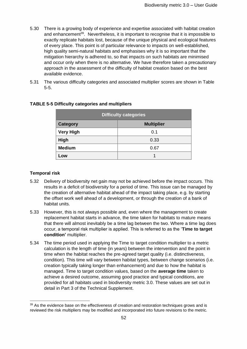
Biodiversity metric 3.0 – User Guide
52
5.30 There is a growing body of experience and expertise associated with habitat creation
and enhancement39. Nevertheless, it is important to recognise that it is impossible to
exactly replicate habitats lost, because of the unique physical and ecological features
of every place. This point is of particular relevance to impacts on well-established,
high quality semi-natural habitats and emphasises why it is so important that the
mitigation hierarchy is adhered to, so that impacts on such habitats are minimised
and occur only when there is no alternative. We have therefore taken a precautionary
approach in the assessment of the difficulty of habitat creation based on the best
available evidence.
5.31 The various difficulty categories and associated multiplier scores are shown in Table
5-5.
TABLE 5-5 Difficulty categories and multipliers
Difficulty categories
Category Multiplier
Very High 0.1
High 0.33
Medium 0.67
Low 1
Temporal risk
5.32 Delivery of biodiversity net gain may not be achieved before the impact occurs. This
results in a deficit of biodiversity for a period of time. This issue can be managed by
the creation of alternative habitat ahead of the impact taking place, e.g. by starting
the offset work well ahead of a development, or through the creation of a bank of
habitat units.
5.33 However, this is not always possible and, even where the management to create
replacement habitat starts in advance, the time taken for habitats to mature means
that there will almost inevitably be a time lag between the two. Where a time lag does
occur, a temporal risk multiplier is applied. This is referred to as the ‘Time to target
condition’ multiplier.
5.34 The time period used in applying the Time to target condition multiplier to a metric
calculation is the length of time (in years) between the intervention and the point in
time when the habitat reaches the pre-agreed target quality (i.e. distinctiveness,
condition). This time will vary between habitat types, between change scenarios (i.e.
creation typically taking longer than enhancement) and due to how the habitat is
managed. Time to target condition values, based on the average time taken to
achieve a desired outcome, assuming good practice and typical conditions, are
provided for all habitats used in biodiversity metric 3.0. These values are set out in
detail in Part 3 of the Technical Supplement.
39 As the evidence base on the effectiveness of creation and restoration techniques grows and is reviewed the risk multipliers may be modified and incorporated into future revisions to the metric.
Biodiversity metric 3.0 – User Guide
53
5.35 These times to target condition have a ‘discounting rate’ applied to them to generate
the multiplier value which is used in biodiversity metric 3.0. ‘Discounting’ over time is
an economic technique used to compare costs and benefits that occur in different
time periods based around the principle that, generally, people prefer to receive
goods and services now rather than later. Where time discounting is used a standard
discount rate is typically applied. Biodiversity metric 3.0 uses 3.5%, which is the value
recommended in the Treasury Green Book40. Table 5-6 shows the multipliers for a
number of time periods between one and 30 years, using a discount rate of 3.5 %. It
is important to use precise figures (at least to three decimal places).
5.36 Biodiversity metric 3.0:
• assumes a quality ‘jump’ from the baseline condition to the target condition
once the relevant number of years have elapsed. Metric calculations do not take
into account incremental increases in quality of the habitat and do not need to be
re-calculated annually, and
• sets a limit on the discount rate used for temporal risk. The metric sets a
multiplier limit of x 0.320 to take account of temporal risk. This equates to a
period of +30 years, which is the maximum time frame that most projects and
plans can realistically plan ahead, and beyond which the multiplier reduces very
slowly. This +30-year value is applied to all scenarios where the time required to
reach the target condition exceeds 30 years. If the time for habitat to reach target
condition exceeds 30 years consider if this is the most appropriate intervention.
5.37 Monitoring is required, to confirm the actual habitat type and condition achieved, and
hence the number of biodiversity units delivered, matches that which was predicted.
40 more details on discounting can be found in The Green Book Guidance, HM Treasury, 2020).
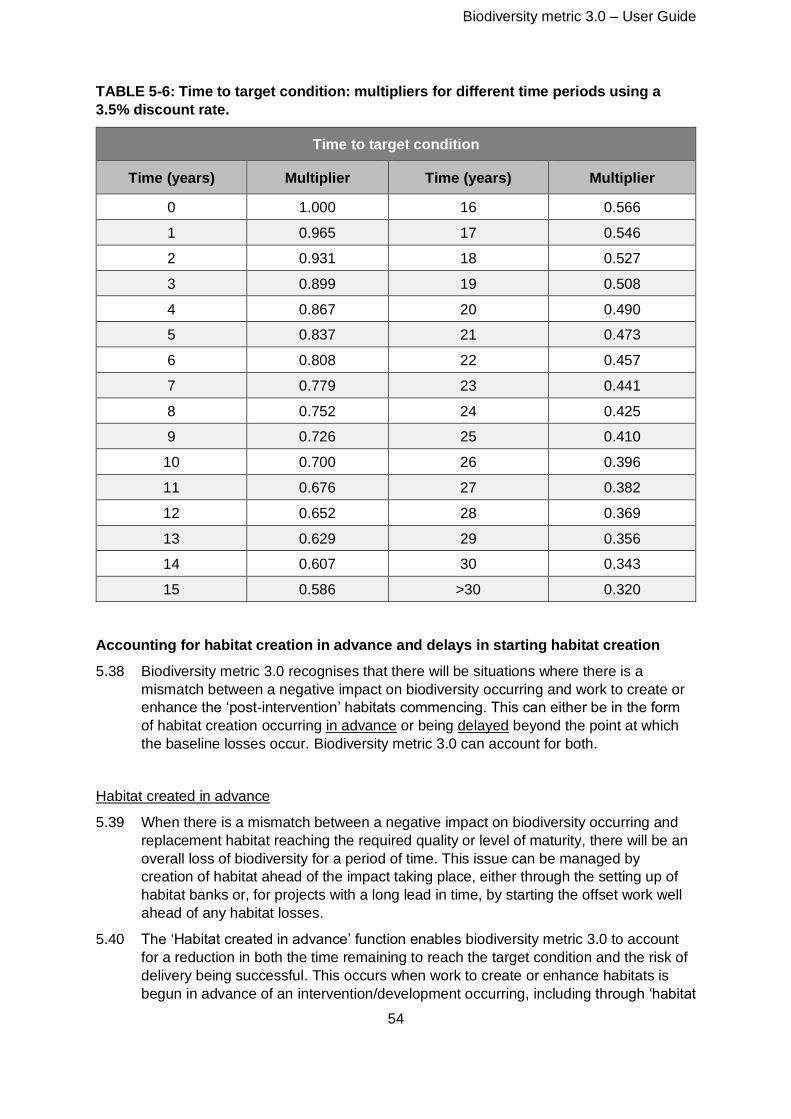
Biodiversity metric 3.0 – User Guide
54
TABLE 5-6: Time to target condition: multipliers for different time periods using a
3.5% discount rate.
Time to target condition
Time (years) Multiplier Time (years) Multiplier
0 1.000 16 0.566
1 0.965 17 0.546
2 0.931 18 0.527
3 0.899 19 0.508
4 0.867 20 0.490
5 0.837 21 0.473
6 0.808 22 0.457
7 0.779 23 0.441
8 0.752 24 0.425
9 0.726 25 0.410
10 0.700 26 0.396
11 0.676 27 0.382
12 0.652 28 0.369
13 0.629 29 0.356
14 0.607 30 0.343
15 0.586 >30 0.320
Accounting for habitat creation in advance and delays in starting habitat creation
5.38 Biodiversity metric 3.0 recognises that there will be situations where there is a
mismatch between a negative impact on biodiversity occurring and work to create or
enhance the ‘post-intervention’ habitats commencing. This can either be in the form
of habitat creation occurring in advance or being delayed beyond the point at which
the baseline losses occur. Biodiversity metric 3.0 can account for both.
Habitat created in advance
5.39 When there is a mismatch between a negative impact on biodiversity occurring and
replacement habitat reaching the required quality or level of maturity, there will be an
overall loss of biodiversity for a period of time. This issue can be managed by
creation of habitat ahead of the impact taking place, either through the setting up of
habitat banks or, for projects with a long lead in time, by starting the offset work well
ahead of any habitat losses.
5.40 The ‘Habitat created in advance’ function enables biodiversity metric 3.0 to account
for a reduction in both the time remaining to reach the target condition and the risk of
delivery being successful. This occurs when work to create or enhance habitats is
begun in advance of an intervention/development occurring, including through ‘habitat
Biodiversity metric 3.0 – User Guide
55
banks’. It recognises that there will be a lower risk of failure following the initial
establishment of a habitat.
5.41 The metric calculation tool reduces the time to target condition by the appropriate
number of years since habitat creation or enhancement began and applies the
adjusted multiplier. If the number of years created in advance is between one and the
time to reach poor condition for that habitat the ‘difficulty of creation’ multiplier will
continue to be applied. However, if the time to reach poor condition has already been
reached or exceeded then the ‘difficulty of enhancement’ multiplier will be applied
instead. If the final time to create the desired habitat type and target condition has
already been reached, then both the time to target condition and the difficulty of
creation risk multipliers will no longer be applied (see Box 5-2).
5.42 Evidence of the habitat advanced habitat creation or enhancement should be
provided and approved by the determining authority and should be referenced in the
‘assessor comments’ cell in the metric. Particularly where the standard time to target
condition for habitat creation is 30+ years evidence will be required to justify that the
proposed condition can be reached in the reduced time.
5.43 This function is available for both on and off-site delivery and for area and linear
habitats.
Delay in starting habitat creation
5.44 There will be circumstances where work to create or enhance the proposed ‘post-
intervention’ habitats cannot commence at the time of the negative impact on
biodiversity occurring. This is most likely to happen with on-site habitat creation,
where the area of land allocated for habitat creation is unavailable due to a
development taking place and the habitat creation/restoration cannot begin until the
development is complete. For example, where the proposed habitat creation is on the
route of an existing road which cannot be removed until the new road is completed or
where it is being used as a site compound for a long period of time.
5.45 When habitat creation is delayed significantly beyond the point at which the baseline
losses occur the ‘Delay in starting habitat creation’ function enables biodiversity
metric 3.0 to account for the resulting increase in the time remaining to reach the
target condition. This function recognises that the risk of failure remains the same as
when habitat creation begins concurrently with the loss, so the difficulty risk multiplier
is applied.
5.46 The metric calculation tool increases the ‘time to target condition’ by the appropriate
number of years that the habitat creation is delayed and applies the adjusted
multiplier. If the number of years delay, combined with the “standard’ time to target
condition applied in metric 3.0, exceeds 30 years then the 30+ years multiplier will be
applied (see Box 5-2).
5.47 This function is available for both on and off-site delivery and for area and linear
habitats.
(Note: Only one of these options may be used for any row in the metric. An error
message will be generated if values are entered for both creation in advance and
delay.)
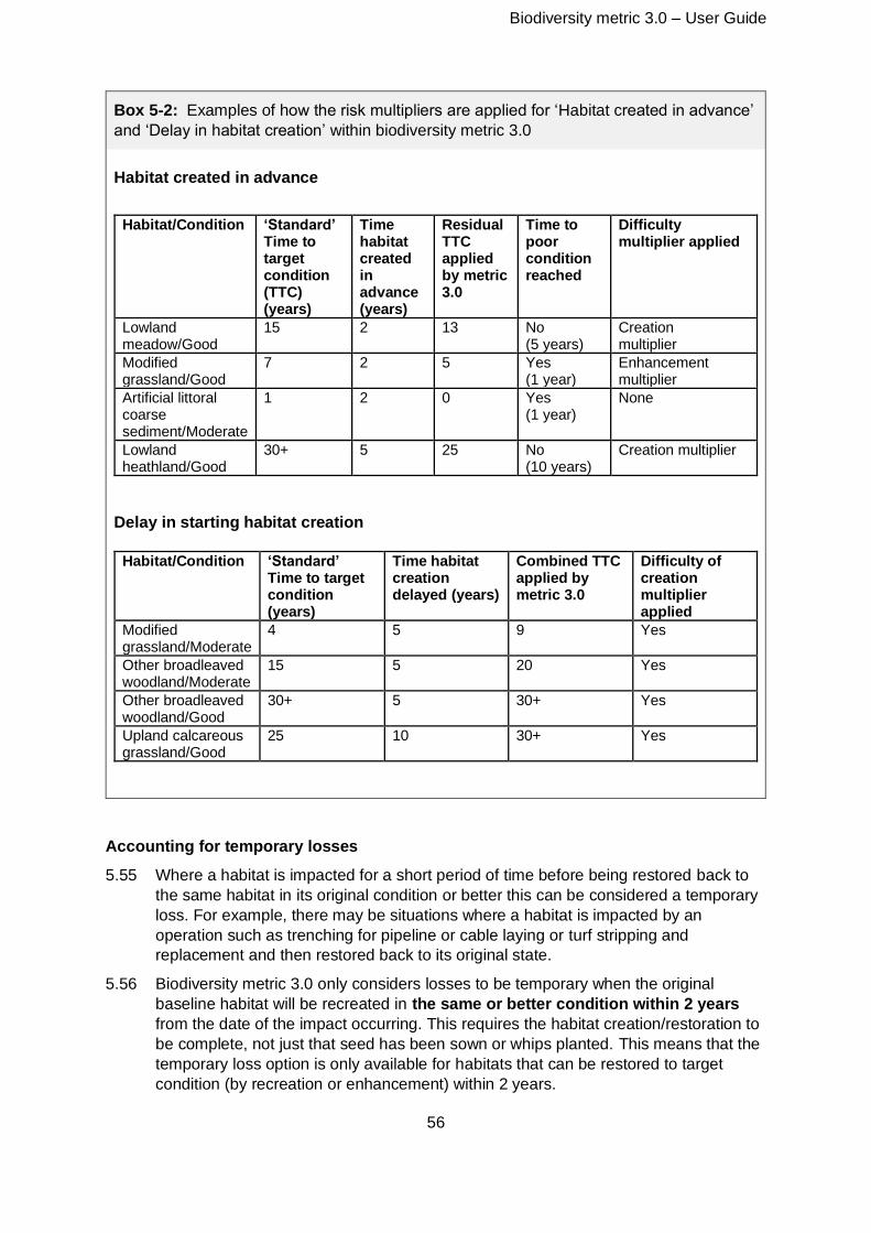
Biodiversity metric 3.0 – User Guide
56
Box 5-2: Examples of how the risk multipliers are applied for ‘Habitat created in advance’
and ‘Delay in habitat creation’ within biodiversity metric 3.0
Habitat created in advance
Habitat/Condition ‘Standard’ Time to target condition (TTC) (years)
Time habitat created in advance (years)
Residual TTC applied by metric 3.0
Time to poor condition reached
Difficulty multiplier applied
Lowland meadow/Good
15 2 13 No (5 years)
Creation multiplier
Modified grassland/Good
7 2 5 Yes (1 year)
Enhancement multiplier
Artificial littoral coarse sediment/Moderate
1 2 0 Yes (1 year)
None
Lowland heathland/Good
30+ 5 25 No (10 years)
Creation multiplier
Delay in starting habitat creation
Habitat/Condition ‘Standard’ Time to target condition (years)
Time habitat creation delayed (years)
Combined TTC applied by metric 3.0
Difficulty of creation multiplier applied
Modified grassland/Moderate
4 5 9 Yes
Other broadleaved woodland/Moderate
15 5 20 Yes
Other broadleaved woodland/Good
30+ 5 30+ Yes
Upland calcareous grassland/Good
25 10 30+ Yes
Accounting for temporary losses
5.55 Where a habitat is impacted for a short period of time before being restored back to
the same habitat in its original condition or better this can be considered a temporary
loss. For example, there may be situations where a habitat is impacted by an
operation such as trenching for pipeline or cable laying or turf stripping and
replacement and then restored back to its original state.
5.56 Biodiversity metric 3.0 only considers losses to be temporary when the original
baseline habitat will be recreated in the same or better condition within 2 years
from the date of the impact occurring. This requires the habitat creation/restoration to
be complete, not just that seed has been sown or whips planted. This means that the
temporary loss option is only available for habitats that can be restored to target
condition (by recreation or enhancement) within 2 years.
Biodiversity metric 3.0 – User Guide
57
5.57 In these situations, it will not be necessary to record the loss within the metric and the
habitat should be recorded as ‘retained’. Where the loss is for a period greater than 2
years, even when the same habitat is restored in the same location, you should
record this as a loss of baseline habitat and creation of the replacement habitat.
Spatial risk
5.58 There are two spatial components in biodiversity metric 3.0. Firstly, strategic
significance describes a site’s location in relation to other habitats and is applied to
both pre- and post-intervention calculations. Secondly, Spatial risk reflects the
relationship between the location in which a biodiversity loss is occurring and that
where the off-site habitat is being delivered. This risk factor is only applied to the off-
site post-intervention calculations.
5.59 There are both ecological and social drivers for off-site habitat to be provided close to
where losses occur: e.g. to avoid depleting biodiversity in local areas or to recognise
the cultural ecosystem services provided by an area of land to a local community. For
this reason, the metric penalises proposals where the off-site habitat is located at
distance from the impact site. The Spatial risk multiplier is applied to those off-site
habitats which are delivered outside either the local planning authority area (LPA), the
same National Character Area (NCA)41 or Marine Plan Area for intertidal habitats.
For rivers and streams the waterbody or catchment is the defining boundary and
WFD waterbody and catchment boundaries should be used to determine the Spatial
risk created by delivering offsets in different locations42.
5.60 Table 5-7 shows the different spatial categories and associated risk scores for
different habitat groupings within biodiversity metric 3.0.
5.61 Those who only wish to use the metric to calculate the biodiversity value of proposed
off-site habitat creation and enhancement, such as landowners wishing to offer
biodiversity units for sale, should enter their data (baseline and post-intervention) into
the on-site tabs in biodiversity metric 3.0. When these biodiversity units are identified
as the off-site biodiversity units for a development or project the developer should
enter this information into the off-site tabs in biodiversity metric 3.0 and must apply
the appropriate spatial risk multiplier to reflect the distance from the site where the
losses are occurring.
41 Further information on NCAs can be found at: http://publications.naturalengland.org.uk/category/587130
42 For those rivers and streams too small to form a WFD waterbody in their own right, the ‘waterbody’
would be defined as the waterbody that the tributary feeds into.
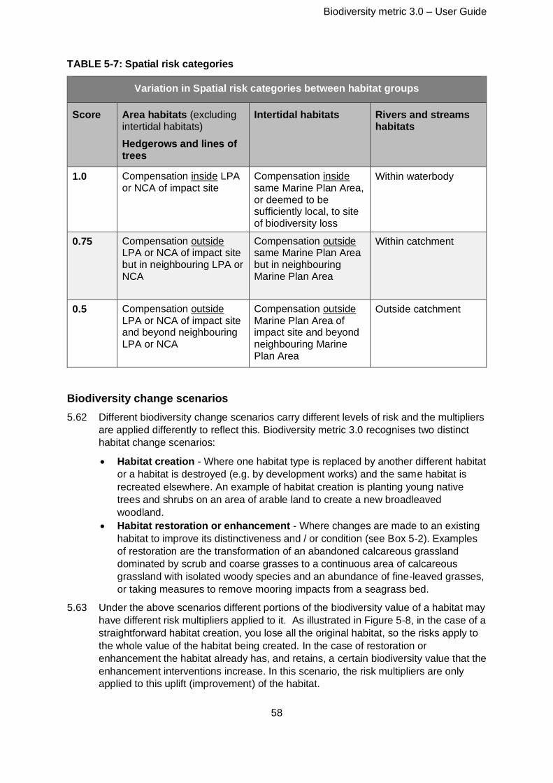
Biodiversity metric 3.0 – User Guide
58
TABLE 5-7: Spatial risk categories
Variation in Spatial risk categories between habitat groups
Score Area habitats (excluding intertidal habitats)
Hedgerows and lines of trees
Intertidal habitats Rivers and streams habitats
1.0 Compensation inside LPA or NCA of impact site
Compensation inside same Marine Plan Area, or deemed to be sufficiently local, to site of biodiversity loss
Within waterbody
0.75 Compensation outside LPA or NCA of impact site but in neighbouring LPA or NCA
Compensation outside same Marine Plan Area but in neighbouring Marine Plan Area
Within catchment
0.5 Compensation outside LPA or NCA of impact site and beyond neighbouring LPA or NCA
Compensation outside Marine Plan Area of impact site and beyond neighbouring Marine Plan Area
Outside catchment
Biodiversity change scenarios
5.62 Different biodiversity change scenarios carry different levels of risk and the multipliers
are applied differently to reflect this. Biodiversity metric 3.0 recognises two distinct
habitat change scenarios:
• Habitat creation - Where one habitat type is replaced by another different habitat
or a habitat is destroyed (e.g. by development works) and the same habitat is
recreated elsewhere. An example of habitat creation is planting young native
trees and shrubs on an area of arable land to create a new broadleaved
woodland.
• Habitat restoration or enhancement - Where changes are made to an existing
habitat to improve its distinctiveness and / or condition (see Box 5-2). Examples
of restoration are the transformation of an abandoned calcareous grassland
dominated by scrub and coarse grasses to a continuous area of calcareous
grassland with isolated woody species and an abundance of fine-leaved grasses,
or taking measures to remove mooring impacts from a seagrass bed.
5.63 Under the above scenarios different portions of the biodiversity value of a habitat may
have different risk multipliers applied to it. As illustrated in Figure 5-8, in the case of a
straightforward habitat creation, you lose all the original habitat, so the risks apply to
the whole value of the habitat being created. In the case of restoration or
enhancement the habitat already has, and retains, a certain biodiversity value that the
enhancement interventions increase. In this scenario, the risk multipliers are only
applied to this uplift (improvement) of the habitat.
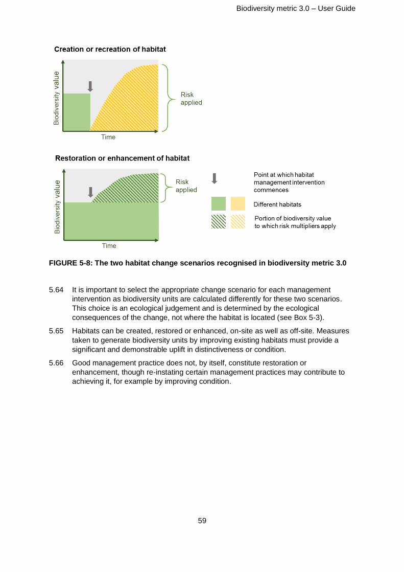
Biodiversity metric 3.0 – User Guide
59
FIGURE 5-8: The two habitat change scenarios recognised in biodiversity metric 3.0
5.64 It is important to select the appropriate change scenario for each management
intervention as biodiversity units are calculated differently for these two scenarios.
This choice is an ecological judgement and is determined by the ecological
consequences of the change, not where the habitat is located (see Box 5-3).
5.65 Habitats can be created, restored or enhanced, on-site as well as off-site. Measures
taken to generate biodiversity units by improving existing habitats must provide a
significant and demonstrable uplift in distinctiveness or condition.
5.66 Good management practice does not, by itself, constitute restoration or
enhancement, though re-instating certain management practices may contribute to
achieving it, for example by improving condition.
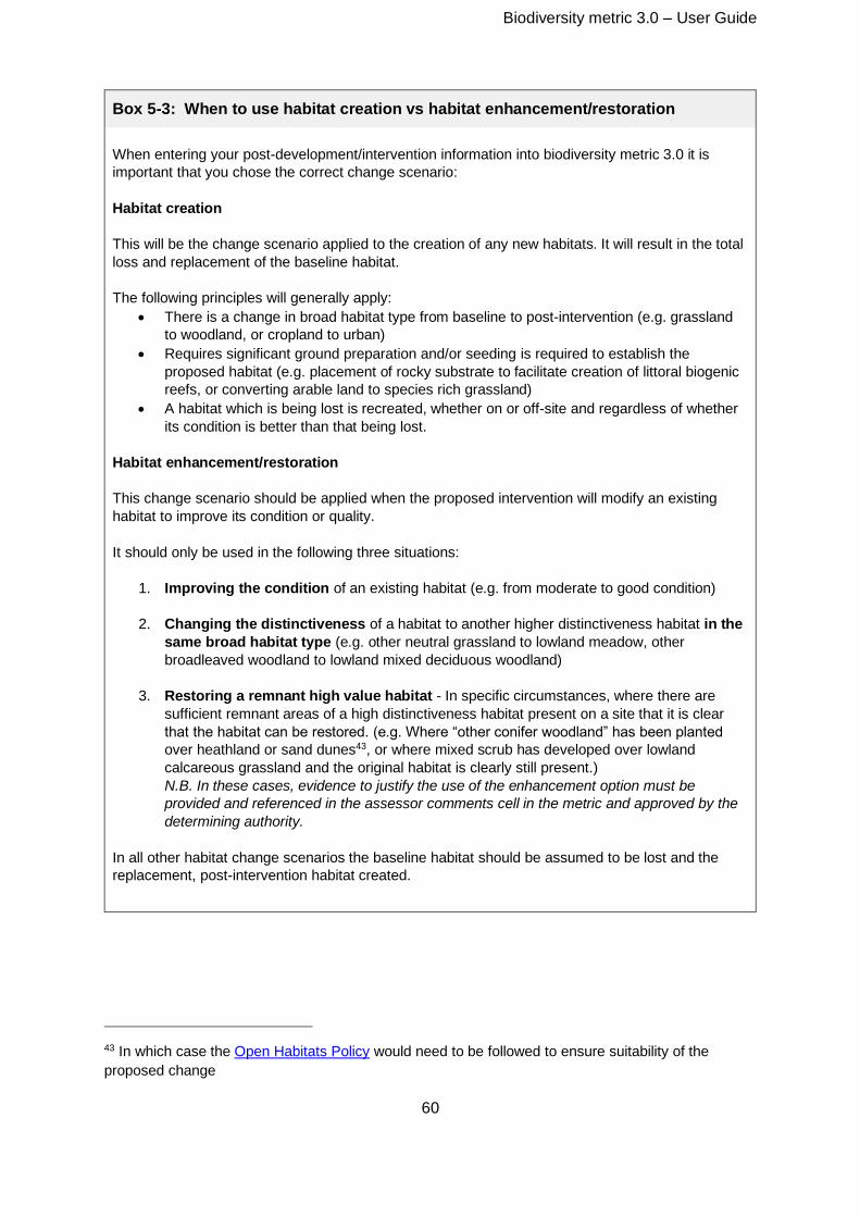
Biodiversity metric 3.0 – User Guide
60
Box 5-3: When to use habitat creation vs habitat enhancement/restoration
When entering your post-development/intervention information into biodiversity metric 3.0 it is
important that you chose the correct change scenario:
Habitat creation
This will be the change scenario applied to the creation of any new habitats. It will result in the total
loss and replacement of the baseline habitat.
The following principles will generally apply:
• There is a change in broad habitat type from baseline to post-intervention (e.g. grassland
to woodland, or cropland to urban)
• Requires significant ground preparation and/or seeding is required to establish the
proposed habitat (e.g. placement of rocky substrate to facilitate creation of littoral biogenic
reefs, or converting arable land to species rich grassland)
• A habitat which is being lost is recreated, whether on or off-site and regardless of whether
its condition is better than that being lost.
Habitat enhancement/restoration
This change scenario should be applied when the proposed intervention will modify an existing
habitat to improve its condition or quality.
It should only be used in the following three situations:
1. Improving the condition of an existing habitat (e.g. from moderate to good condition)
2. Changing the distinctiveness of a habitat to another higher distinctiveness habitat in the
same broad habitat type (e.g. other neutral grassland to lowland meadow, other
broadleaved woodland to lowland mixed deciduous woodland)
3. Restoring a remnant high value habitat - In specific circumstances, where there are
sufficient remnant areas of a high distinctiveness habitat present on a site that it is clear
that the habitat can be restored. (e.g. Where “other conifer woodland” has been planted
over heathland or sand dunes43, or where mixed scrub has developed over lowland
calcareous grassland and the original habitat is clearly still present.)
N.B. In these cases, evidence to justify the use of the enhancement option must be
provided and referenced in the assessor comments cell in the metric and approved by the
determining authority.
In all other habitat change scenarios the baseline habitat should be assumed to be lost and the
replacement, post-intervention habitat created.
43 In which case the Open Habitats Policy would need to be followed to ensure suitability of the
proposed change
Biodiversity metric 3.0 – User Guide
61
6: Area habitat biodiversity unit calculations
6.1 Areas habitats are perhaps the most familiar ecological currency in the UK. They are
the woodlands, grasslands, wetlands, coastal, intertidal and other habitat types that
are widely recognised by ecologists and the public alike. The habitats we recognise
comprise a community of different species populations living in a place. There is
usually a sub-group of those populations that give a habitat its defining
characteristics, for example trees in a woodland or grasses in a meadow.
6.2 There are a variety of habitat classification systems available in the UK, for example
Phase 144, UKHab45 and EUNIS46. Biodiversity metric 3.0 uses a combination of
these: UKHab for the majority of area habitats, EUNIS for intertidal habitats and WFD
lakes typologies for lakes. There are a small number of habitats which have specific
biodiversity metric 3.0 definitions (see Table TS2-1).
6.3 UKHab is a unified and comprehensive habitat classification coding system for all
terrestrial, freshwater and marine habitats in the UK, designed to provide a simple
and robust approach to survey and monitoring and which includes a detailed
nomenclature for urban areas. It is flexible enough for use in a wide range of survey
types from walkover surveys of small urban sites to regional and national scale rural
habitat mapping.
6.4 EUNIS is a comprehensive system developed to facilitate the harmonised description
and collection of data across Europe; it covers all habitats types from natural to
artificial, and through to the marine (subtidal) environment. The EUNIS habitat
classification system is the habitat classification used in reporting across the marine
environment in Europe. Alkalinity is the basis of the WFD lakes typology along with
peat and marl. Nearly all lakes above 2 ha have already been assigned to one of the
WFD types using either measured or modelled data. These types can be found on
the UK lakes portal47.
6.5 Calculating the baseline biodiversity unit value of a site uses the area, distinctiveness,
condition and strategic significance of each habitat.
Distinctiveness
6.6 As described in Chapter 5, distinctiveness refers to the relative scarcity of a habitat
and its importance for nature conservation. The distinctiveness categories used for
Area Habitats and examples illustrating the types of habitats assigned to each
category are shown in Table 5-1. The distinctiveness category assigned to each
habitat type used in biodiversity metric 3.0 is provided in part 2 of the Technical
Supplement. (Tables TS2-6 to TS2-17 and summarised in Table TS3-1).
6.7 The distinctiveness band of a habitat will affect its biodiversity unit value. A higher
distinctiveness has the effect of increasing the biodiversity unit score for a habitat in
44 JNCC (2010) Handbook for Phase 1 habitat survey - a technique for environmental audit (revised 2010) 45 UK Habitat Classification: https://ukhab.org/
46 European Nature Information System
47 UK lakes portal
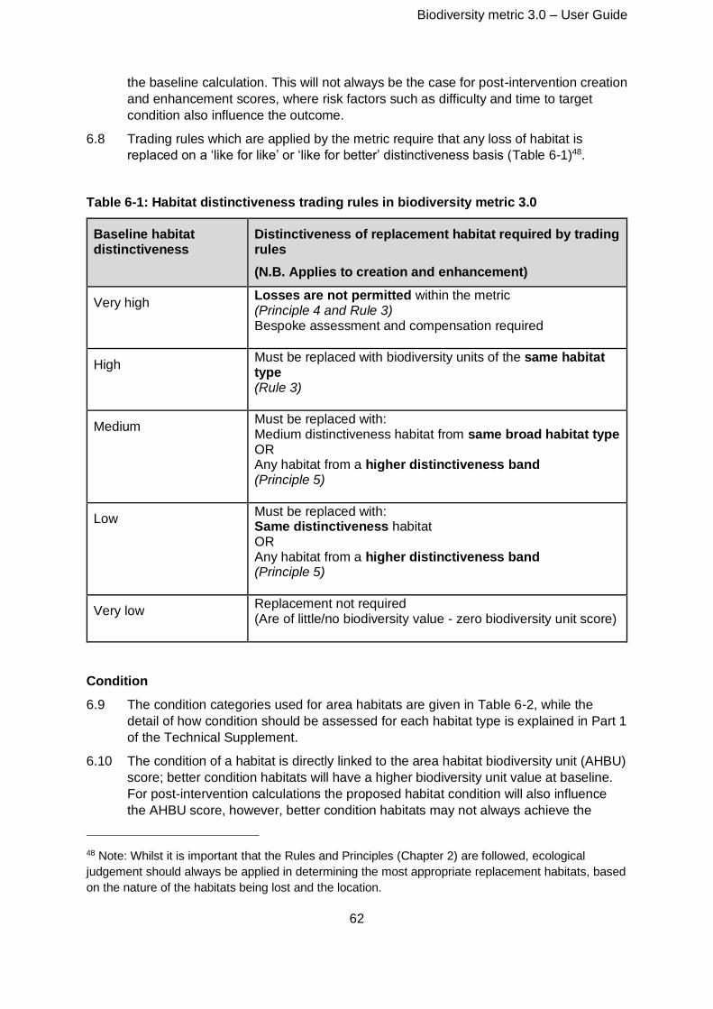
Biodiversity metric 3.0 – User Guide
62
the baseline calculation. This will not always be the case for post-intervention creation
and enhancement scores, where risk factors such as difficulty and time to target
condition also influence the outcome.
6.8 Trading rules which are applied by the metric require that any loss of habitat is
replaced on a ‘like for like’ or ‘like for better’ distinctiveness basis (Table 6-1)48.
Table 6-1: Habitat distinctiveness trading rules in biodiversity metric 3.0
Baseline habitat distinctiveness
Distinctiveness of replacement habitat required by trading rules
(N.B. Applies to creation and enhancement)
Very high Losses are not permitted within the metric (Principle 4 and Rule 3) Bespoke assessment and compensation required
High Must be replaced with biodiversity units of the same habitat type (Rule 3)
Medium Must be replaced with: Medium distinctiveness habitat from same broad habitat type OR Any habitat from a higher distinctiveness band (Principle 5)
Low Must be replaced with: Same distinctiveness habitat OR Any habitat from a higher distinctiveness band (Principle 5)
Very low Replacement not required (Are of little/no biodiversity value - zero biodiversity unit score)
Condition
6.9 The condition categories used for area habitats are given in Table 6-2, while the
detail of how condition should be assessed for each habitat type is explained in Part 1
of the Technical Supplement.
6.10 The condition of a habitat is directly linked to the area habitat biodiversity unit (AHBU)
score; better condition habitats will have a higher biodiversity unit value at baseline.
For post-intervention calculations the proposed habitat condition will also influence
the AHBU score, however, better condition habitats may not always achieve the
48 Note: Whilst it is important that the Rules and Principles (Chapter 2) are followed, ecological
judgement should always be applied in determining the most appropriate replacement habitats, based
on the nature of the habitats being lost and the location.
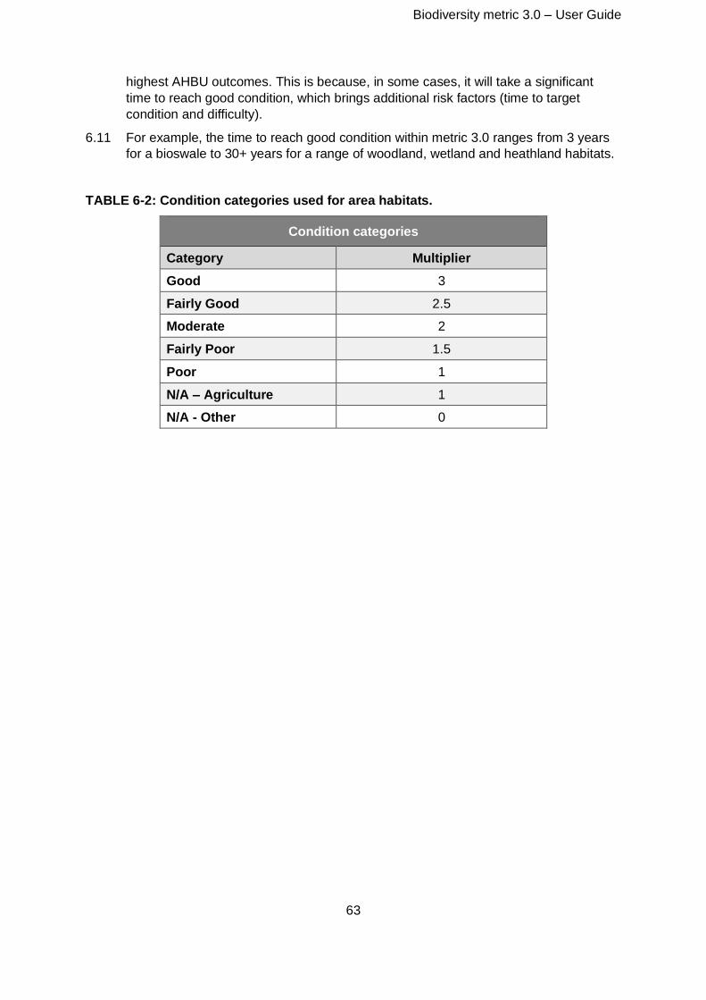
Biodiversity metric 3.0 – User Guide
63
highest AHBU outcomes. This is because, in some cases, it will take a significant
time to reach good condition, which brings additional risk factors (time to target
condition and difficulty).
6.11 For example, the time to reach good condition within metric 3.0 ranges from 3 years
for a bioswale to 30+ years for a range of woodland, wetland and heathland habitats.
TABLE 6-2: Condition categories used for area habitats.
Condition categories
Category Multiplier
Good 3
Fairly Good 2.5
Moderate 2
Fairly Poor 1.5
Poor 1
N/A – Agriculture 1
N/A - Other 0
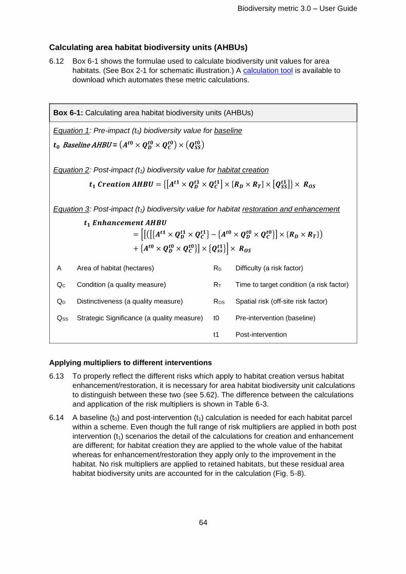
Biodiversity metric 3.0 – User Guide
64
Calculating area habitat biodiversity units (AHBUs)
6.12 Box 6-1 shows the formulae used to calculate biodiversity unit values for area
habitats. (See Box 2-1 for schematic illustration.) A calculation tool is available to
download which automates these metric calculations.
Box 6-1: Calculating area habitat biodiversity units (AHBUs)
Equation 1: Pre-impact (t0) biodiversity value for baseline
𝒕𝟎 Baseline AHBU = (𝑨𝒕𝟎 × 𝑸𝑫𝒕𝟎 × 𝑸𝑪
𝒕𝟎) × (𝑸𝑺𝑺𝒕𝟎 )
Equation 2: Post-impact (t1) biodiversity value for habitat creation
𝒕𝟏 𝑪𝒓𝒆𝒂𝒕𝒊𝒐𝒏 𝑨𝑯𝑩𝑼 = {[𝑨𝒕𝟏 × 𝑸𝑫𝒕𝟏 × 𝑸𝑪
𝒕𝟏] × [𝑹𝑫 × 𝑹𝑻] × [𝑸𝑺𝑺𝒕𝟏 ]} × 𝑹𝑶𝑺
Equation 3: Post-impact (t1) biodiversity value for habitat restoration and enhancement
𝒕𝟏 𝑬𝒏𝒉𝒂𝒏𝒄𝒆𝒎𝒆𝒏𝒕 𝑨𝑯𝑩𝑼
= [[([{𝑨𝒕𝟏 × 𝑸𝑫𝒕𝟏 × 𝑸𝑪
𝒕𝟏} − {𝑨𝒕𝟎 × 𝑸𝑫𝒕𝟎 × 𝑸𝑪
𝒕𝟎}] × {𝑹𝑫 × 𝑹𝑻})
+ {𝑨𝒕𝟎 × 𝑸𝑫𝒕𝟎 × 𝑸𝑪
𝒕𝟎}] × {𝑸𝒔𝒔𝒕𝟏}] × 𝑹𝑶𝑺
A Area of habitat (hectares) RD Difficulty (a risk factor)
QC Condition (a quality measure) RT Time to target condition (a risk factor)
QD Distinctiveness (a quality measure) ROS Spatial risk (off-site risk factor)
QSS Strategic Significance (a quality measure) t0 Pre-intervention (baseline)
t1 Post-intervention
Applying multipliers to different interventions
6.13 To properly reflect the different risks which apply to habitat creation versus habitat
enhancement/restoration, it is necessary for area habitat biodiversity unit calculations
to distinguish between these two (see 5.62). The difference between the calculations
and application of the risk multipliers is shown in Table 6-3.
6.14 A baseline (t0) and post-intervention (t1) calculation is needed for each habitat parcel
within a scheme. Even though the full range of risk multipliers are applied in both post
intervention (t1) scenarios the detail of the calculations for creation and enhancement
are different; for habitat creation they are applied to the whole value of the habitat
whereas for enhancement/restoration they apply only to the improvement in the
habitat. No risk multipliers are applied to retained habitats, but these residual area
habitat biodiversity units are accounted for in the calculation (Fig. 5-8).
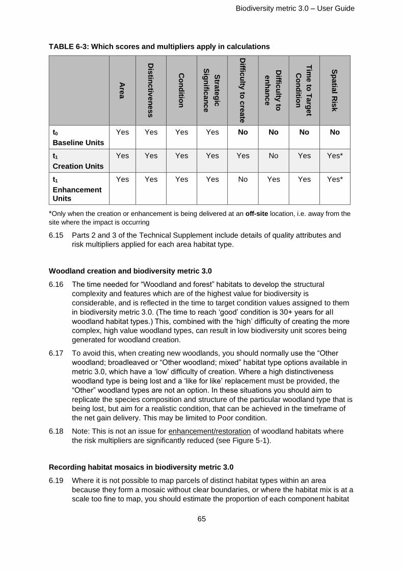
Biodiversity metric 3.0 – User Guide
65
TABLE 6-3: Which scores and multipliers apply in calculations
Are
a
Dis
tinc
tive
ne
ss
Co
nd
ition
Stra
teg
ic
Sig
nific
an
ce
Diffic
ulty
to c
rea
te
Diffic
ulty
to
en
ha
nc
e
Tim
e to
Ta
rge
t
Co
nd
ition
Sp
atia
l Ris
k
t0
Baseline Units
Yes Yes Yes Yes No No No No
t1
Creation Units
Yes Yes Yes Yes Yes No Yes Yes*
t1
Enhancement Units
Yes Yes Yes Yes No Yes Yes Yes*
*Only when the creation or enhancement is being delivered at an off-site location, i.e. away from the
site where the impact is occurring
6.15 Parts 2 and 3 of the Technical Supplement include details of quality attributes and
risk multipliers applied for each area habitat type.
Woodland creation and biodiversity metric 3.0
6.16 The time needed for “Woodland and forest” habitats to develop the structural
complexity and features which are of the highest value for biodiversity is
considerable, and is reflected in the time to target condition values assigned to them
in biodiversity metric 3.0. (The time to reach ‘good’ condition is 30+ years for all
woodland habitat types.) This, combined with the ‘high’ difficulty of creating the more
complex, high value woodland types, can result in low biodiversity unit scores being
generated for woodland creation.
6.17 To avoid this, when creating new woodlands, you should normally use the “Other
woodland; broadleaved or “Other woodland; mixed” habitat type options available in
metric 3.0, which have a ‘low’ difficulty of creation. Where a high distinctiveness
woodland type is being lost and a ‘like for like’ replacement must be provided, the
“Other” woodland types are not an option. In these situations you should aim to
replicate the species composition and structure of the particular woodland type that is
being lost, but aim for a realistic condition, that can be achieved in the timeframe of
the net gain delivery. This may be limited to Poor condition.
6.18 Note: This is not an issue for enhancement/restoration of woodland habitats where
the risk multipliers are significantly reduced (see Figure 5-1).
Recording habitat mosaics in biodiversity metric 3.0
6.19 Where it is not possible to map parcels of distinct habitat types within an area
because they form a mosaic without clear boundaries, or where the habitat mix is at a
scale too fine to map, you should estimate the proportion of each component habitat
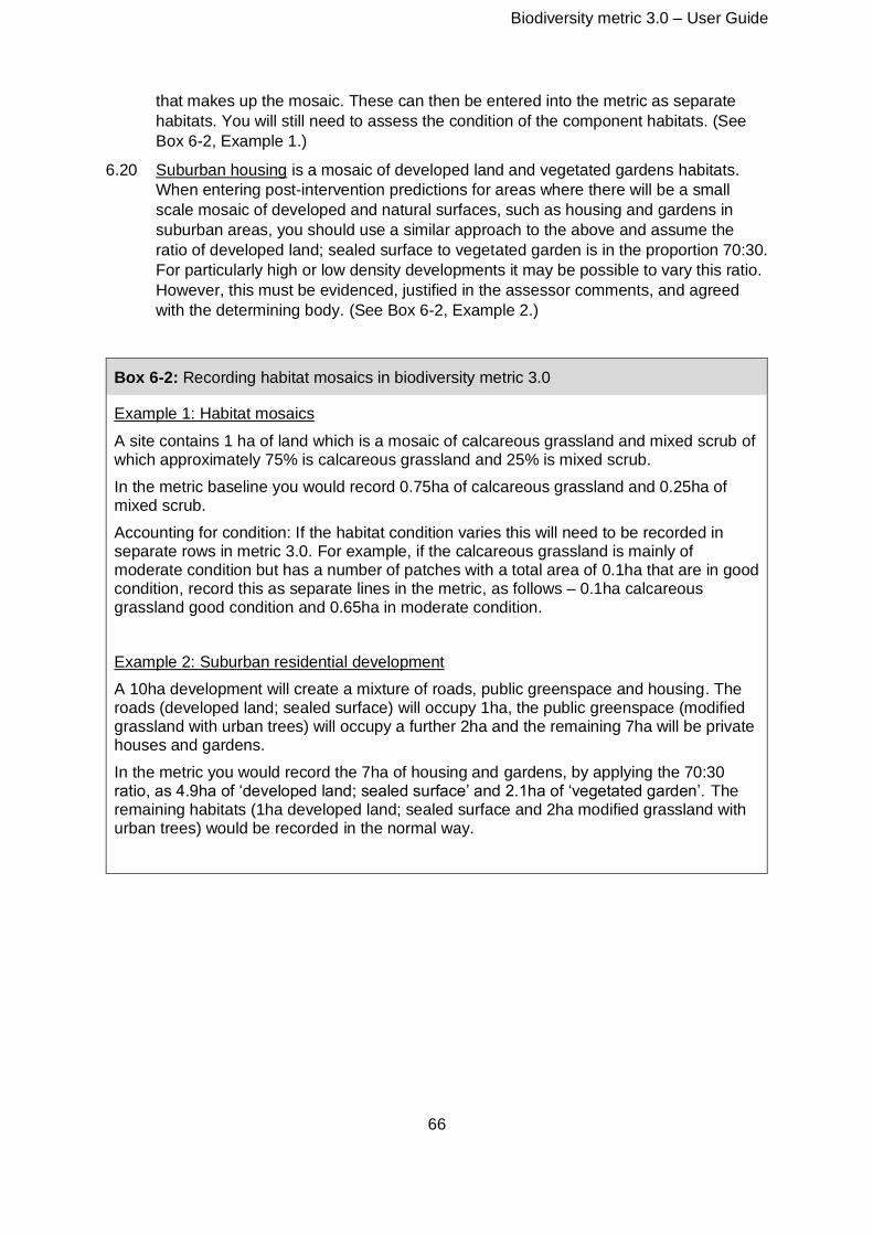
Biodiversity metric 3.0 – User Guide
66
that makes up the mosaic. These can then be entered into the metric as separate
habitats. You will still need to assess the condition of the component habitats. (See
Box 6-2, Example 1.)
6.20 Suburban housing is a mosaic of developed land and vegetated gardens habitats.
When entering post-intervention predictions for areas where there will be a small
scale mosaic of developed and natural surfaces, such as housing and gardens in
suburban areas, you should use a similar approach to the above and assume the
ratio of developed land; sealed surface to vegetated garden is in the proportion 70:30.
For particularly high or low density developments it may be possible to vary this ratio.
However, this must be evidenced, justified in the assessor comments, and agreed
with the determining body. (See Box 6-2, Example 2.)
Box 6-2: Recording habitat mosaics in biodiversity metric 3.0
Example 1: Habitat mosaics
A site contains 1 ha of land which is a mosaic of calcareous grassland and mixed scrub of which approximately 75% is calcareous grassland and 25% is mixed scrub.
In the metric baseline you would record 0.75ha of calcareous grassland and 0.25ha of mixed scrub.
Accounting for condition: If the habitat condition varies this will need to be recorded in separate rows in metric 3.0. For example, if the calcareous grassland is mainly of moderate condition but has a number of patches with a total area of 0.1ha that are in good condition, record this as separate lines in the metric, as follows – 0.1ha calcareous grassland good condition and 0.65ha in moderate condition.
Example 2: Suburban residential development
A 10ha development will create a mixture of roads, public greenspace and housing. The roads (developed land; sealed surface) will occupy 1ha, the public greenspace (modified grassland with urban trees) will occupy a further 2ha and the remaining 7ha will be private houses and gardens.
In the metric you would record the 7ha of housing and gardens, by applying the 70:30 ratio, as 4.9ha of ‘developed land; sealed surface’ and 2.1ha of ‘vegetated garden’. The remaining habitats (1ha developed land; sealed surface and 2ha modified grassland with urban trees) would be recorded in the normal way.
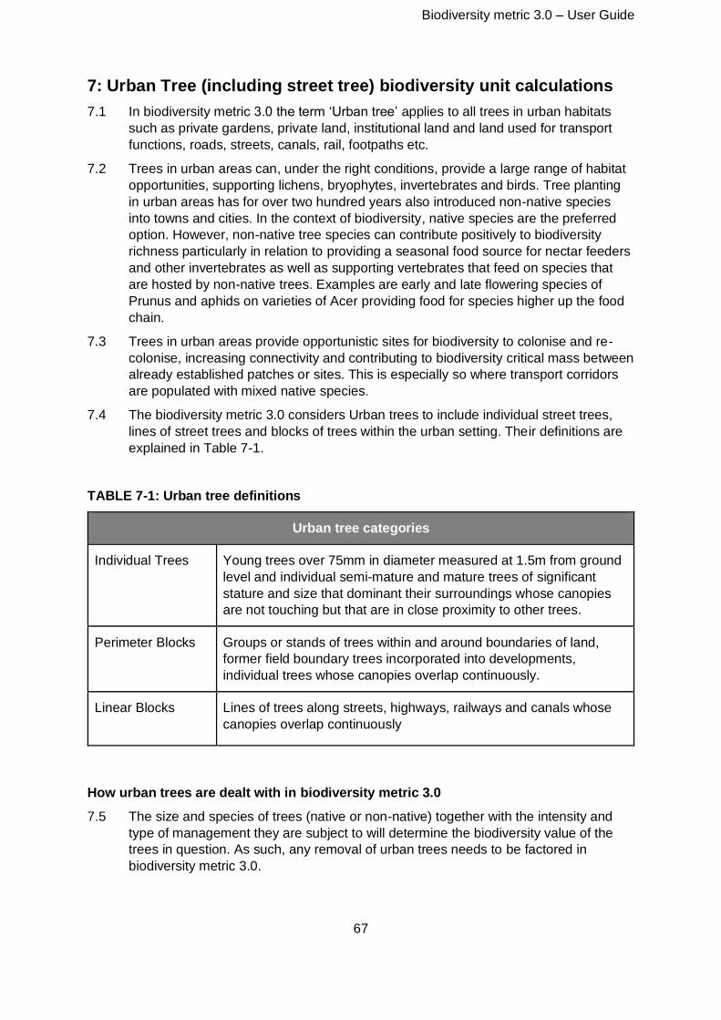
Biodiversity metric 3.0 – User Guide
67
7: Urban Tree (including street tree) biodiversity unit calculations
7.1 In biodiversity metric 3.0 the term ‘Urban tree’ applies to all trees in urban habitats
such as private gardens, private land, institutional land and land used for transport
functions, roads, streets, canals, rail, footpaths etc.
7.2 Trees in urban areas can, under the right conditions, provide a large range of habitat
opportunities, supporting lichens, bryophytes, invertebrates and birds. Tree planting
in urban areas has for over two hundred years also introduced non-native species
into towns and cities. In the context of biodiversity, native species are the preferred
option. However, non-native tree species can contribute positively to biodiversity
richness particularly in relation to providing a seasonal food source for nectar feeders
and other invertebrates as well as supporting vertebrates that feed on species that
are hosted by non-native trees. Examples are early and late flowering species of
Prunus and aphids on varieties of Acer providing food for species higher up the food
chain.
7.3 Trees in urban areas provide opportunistic sites for biodiversity to colonise and re-
colonise, increasing connectivity and contributing to biodiversity critical mass between
already established patches or sites. This is especially so where transport corridors
are populated with mixed native species.
7.4 The biodiversity metric 3.0 considers Urban trees to include individual street trees,
lines of street trees and blocks of trees within the urban setting. Their definitions are
explained in Table 7-1.
TABLE 7-1: Urban tree definitions
Urban tree categories
Individual Trees
Young trees over 75mm in diameter measured at 1.5m from ground
level and individual semi-mature and mature trees of significant
stature and size that dominant their surroundings whose canopies
are not touching but that are in close proximity to other trees.
Perimeter Blocks
Groups or stands of trees within and around boundaries of land,
former field boundary trees incorporated into developments,
individual trees whose canopies overlap continuously.
Linear Blocks
Lines of trees along streets, highways, railways and canals whose
canopies overlap continuously
How urban trees are dealt with in biodiversity metric 3.0
7.5 The size and species of trees (native or non-native) together with the intensity and
type of management they are subject to will determine the biodiversity value of the
trees in question. As such, any removal of urban trees needs to be factored in
biodiversity metric 3.0.
Biodiversity metric 3.0 – User Guide
68
7.6 They require a slightly different approach to the area habitat biodiversity unit
calculation.
7.7 The urban tree tool can also be used to obtain area and biodiversity unit values for
trees outside the urban environment. For example, a tree in the middle of an arable or
grassland field which is a common sight in the British landscape.
Distinctiveness and difficulty of creation and enhancement
7.8 Urban trees have a Medium distinctiveness score in biodiversity metric 3.0 as they
vary in the species that are planted, sit in stressed environments and would only be
considered a single component of a more complex habitat such as woodland.
7.9 They have also been attributed a low difficulty for both creation and enhancement.
Condition assessment
7.10 Urban trees are split into small, medium and large trees and are assessed using an
Urban tree condition assessment proforma to score the trees as Poor (score of 1),
Moderate (score of 2) or Good (Score of 3) condition (see Technical Supplement Part
1a).
7.11 It is important that both size and condition are recorded for each tree. Trees of the
same size and condition can then be grouped together before entry into the ‘Urban
tree helper’ to generate an area equivalent for each condition category. The number
of small, medium and large trees is then automatically converted into a total area
equivalent value which can be used in the metric calculation. (See Box 7-1).
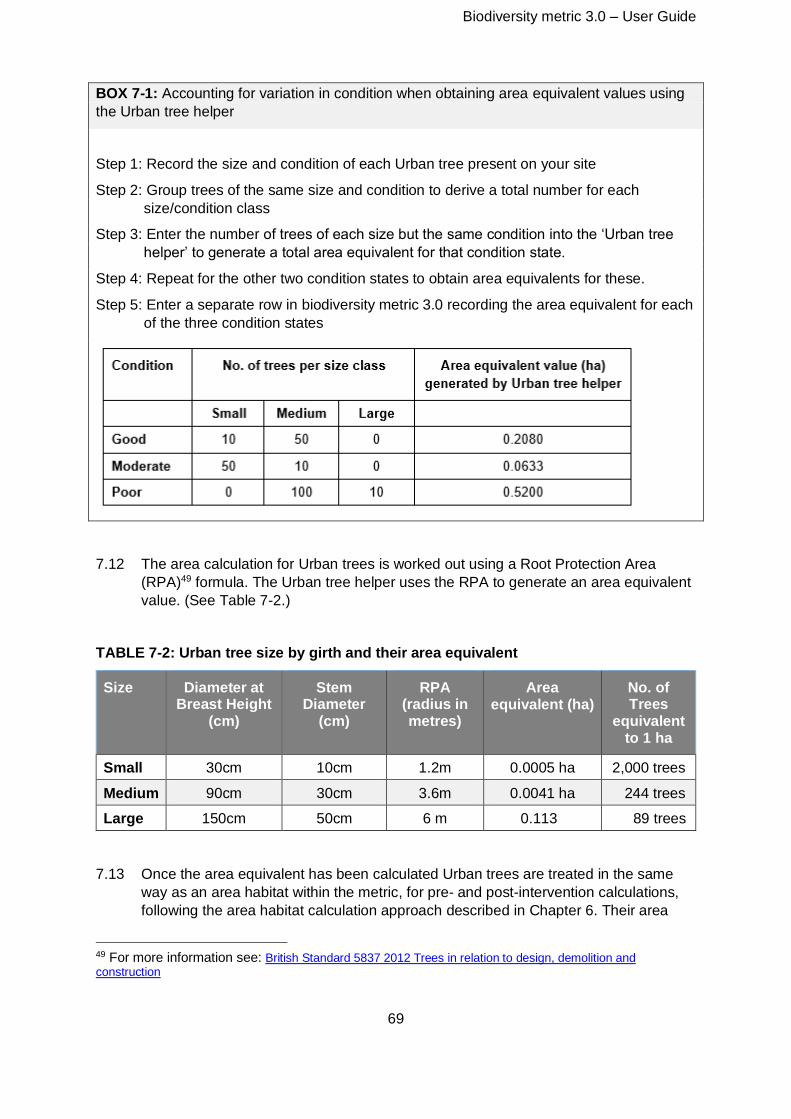
Biodiversity metric 3.0 – User Guide
69
BOX 7-1: Accounting for variation in condition when obtaining area equivalent values using
the Urban tree helper
Step 1: Record the size and condition of each Urban tree present on your site
Step 2: Group trees of the same size and condition to derive a total number for each
size/condition class
Step 3: Enter the number of trees of each size but the same condition into the ‘Urban tree
helper’ to generate a total area equivalent for that condition state.
Step 4: Repeat for the other two condition states to obtain area equivalents for these.
Step 5: Enter a separate row in biodiversity metric 3.0 recording the area equivalent for each
of the three condition states
7.12 The area calculation for Urban trees is worked out using a Root Protection Area
(RPA)49 formula. The Urban tree helper uses the RPA to generate an area equivalent
value. (See Table 7-2.)
TABLE 7-2: Urban tree size by girth and their area equivalent
Size Diameter at Breast Height
(cm)
Stem Diameter
(cm)
RPA (radius in metres)
Area equivalent (ha)
No. of Trees
equivalent to 1 ha
Small 30cm 10cm 1.2m 0.0005 ha 2,000 trees
Medium 90cm 30cm 3.6m 0.0041 ha 244 trees
Large 150cm 50cm 6 m 0.113 89 trees
7.13 Once the area equivalent has been calculated Urban trees are treated in the same
way as an area habitat within the metric, for pre- and post-intervention calculations,
following the area habitat calculation approach described in Chapter 6. Their area
49 For more information see: British Standard 5837 2012 Trees in relation to design, demolition and construction
Biodiversity metric 3.0 – User Guide
70
does not need to be deducted from the total area of other habitats within the site
boundary. It will not generate a total area error.
7.14 The mitigation hierarchy applies and where possible ‘like for like’ compensation is the
preferred approach.
Biodiversity metric 3.0 – User Guide
71
8: Linear habitat biodiversity unit calculations
8.1 Biodiversity metric 3.0 includes separate calculations for linear habitats:
• Hedgerows and lines of trees
• Rivers and streams
8.2 Treating these linear habitats like other habitats and accounting for their biodiversity
value using the area habitat approach would undervalue their importance and would
fail to ensure adequate provision for losses. It is therefore necessary to take separate
account of these habitat types so that their contribution to biodiversity is properly
acknowledged (see 2.7, 2.8 and Rule 4).
8.3 ‘Hedgerow and lines of trees biodiversity units’ (HBUs) are the units used to measure
the biodiversity value of hedgerows and lines of trees and to clearly differentiate from
biodiversity units associated with area habitats (ABHUs) and river and streams
habitats (RBUs).
Hedgerows and lines of trees
8.4 Hedgerows as a linear habitat are a feature almost unique to the British Isles.
Biodiversity metric 3.0 further refines the approach taken for hedgerows in the Defra
biodiversity metric (2012), and Biodiversity metric 2.0 (2019), which both separated
hedgerows from area habitats. ‘Lines of trees’ are included since they display some
of the same functional qualities as hedgerows.
8.5 Urban trees are considered separately to lines of trees in the wider environment,
since they generally occur in an urban environment surrounded by developed land.
For information on how urban trees are considered in biodiversity metric 3.0 see
Chapter 7.
Calculating hedgerows and lines of trees biodiversity units (HBUs)
8.6 Box 8-1 shows the formulae used to calculate biodiversity unit values for hedgerows
and lines of trees.
8.7 To properly reflect the different risks, it is necessary for hedgerow and line of trees
biodiversity unit calculations to distinguish between creation and enhancement (see
5.62). A baseline (t0) and post-intervention (t1) calculation is needed for each
hedgerow or line of trees within a scheme to determine the uplift in biodiversity value.
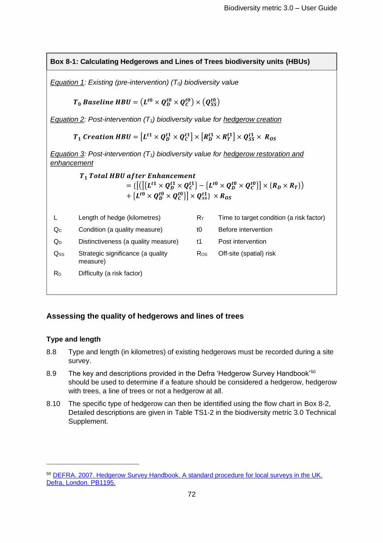
Biodiversity metric 3.0 – User Guide
72
Box 8-1: Calculating Hedgerows and Lines of Trees biodiversity units (HBUs)
Equation 1: Existing (pre-intervention) (T0) biodiversity value
𝑻𝟎 𝑩𝒂𝒔𝒆𝒍𝒊𝒏𝒆 𝑯𝑩𝑼 = (𝑳𝒕𝟎 × 𝑸𝑫𝒕𝟎 × 𝑸𝑪
𝒕𝟎) × (𝑸𝑺𝑺𝒕𝟎 )
Equation 2: Post-intervention (T1) biodiversity value for hedgerow creation
𝑻𝟏 𝑪𝒓𝒆𝒂𝒕𝒊𝒐𝒏 𝑯𝑩𝑼 = [𝑳𝒕𝟏 × 𝑸𝑫𝒕𝟏 × 𝑸𝑪
𝒕𝟏] × [𝑹𝑫𝒕𝟏 × 𝑹𝑻
𝒕𝟏] × 𝑸𝑺𝑺𝒕𝟏 × 𝑹𝑶𝑺
Equation 3: Post-intervention (T1) biodiversity value for hedgerow restoration and
enhancement
𝑻𝟏 𝑻𝒐𝒕𝒂𝒍 𝑯𝑩𝑼 𝒂𝒇𝒕𝒆𝒓 𝑬𝒏𝒉𝒂𝒏𝒄𝒆𝒎𝒆𝒏𝒕
= {[([{𝑳𝒕𝟏 × 𝑸𝑫𝒕𝟏 × 𝑸𝑪
𝒕𝟏} − {𝑳𝒕𝟎 × 𝑸𝑫𝒕𝟎 × 𝑸𝑪
𝒕𝟎}] × {𝑹𝑫 × 𝑹𝑻})
+ {𝑳𝒕𝟎 × 𝑸𝑫𝒕𝟎 × 𝑸𝑪
𝒕𝟎}] × 𝑸𝒔𝒔𝒕𝟏} × 𝑹𝑶𝑺
L Length of hedge (kilometres) RT Time to target condition (a risk factor)
QC Condition (a quality measure) t0 Before intervention
QD Distinctiveness (a quality measure) t1 Post intervention
QSS Strategic significance (a quality
measure)
ROS Off-site (spatial) risk
RD Difficulty (a risk factor)
Assessing the quality of hedgerows and lines of trees
Type and length
8.8 Type and length (in kilometres) of existing hedgerows must be recorded during a site
survey.
8.9 The key and descriptions provided in the Defra ‘Hedgerow Survey Handbook’50
should be used to determine if a feature should be considered a hedgerow, hedgerow
with trees, a line of trees or not a hedgerow at all.
8.10 The specific type of hedgerow can then be identified using the flow chart in Box 8-2,
Detailed descriptions are given in Table TS1-2 in the biodiversity metric 3.0 Technical
Supplement.
50 DEFRA. 2007. Hedgerow Survey Handbook. A standard procedure for local surveys in the UK. Defra, London. PB1195.
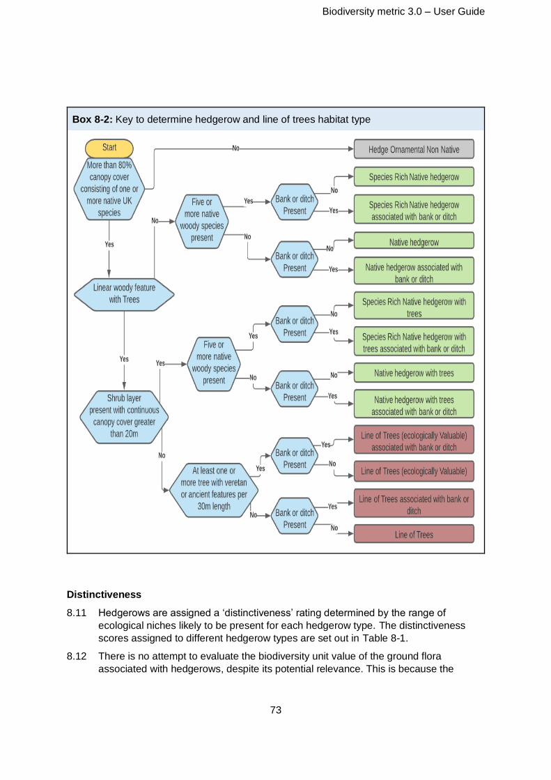
Biodiversity metric 3.0 – User Guide
73
Box 8-2: Key to determine hedgerow and line of trees habitat type
Distinctiveness
8.11 Hedgerows are assigned a ‘distinctiveness’ rating determined by the range of
ecological niches likely to be present for each hedgerow type. The distinctiveness
scores assigned to different hedgerow types are set out in Table 8-1.
8.12 There is no attempt to evaluate the biodiversity unit value of the ground flora
associated with hedgerows, despite its potential relevance. This is because the
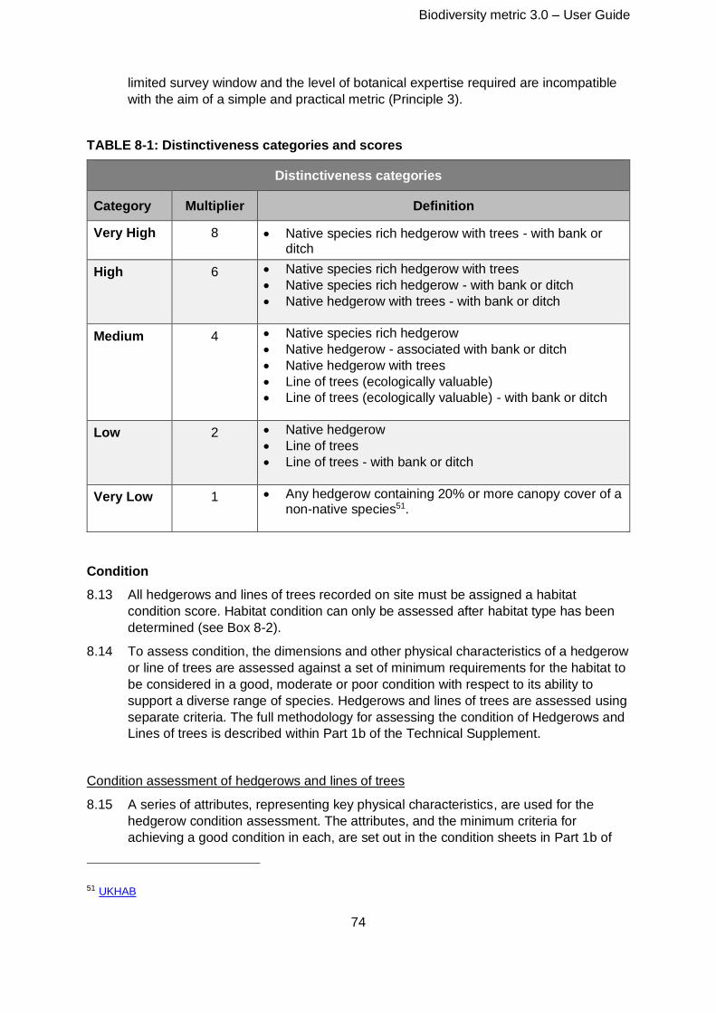
Biodiversity metric 3.0 – User Guide
74
limited survey window and the level of botanical expertise required are incompatible
with the aim of a simple and practical metric (Principle 3).
TABLE 8-1: Distinctiveness categories and scores
Distinctiveness categories
Category Multiplier Definition
Very High 8 • Native species rich hedgerow with trees - with bank or ditch
High 6 • Native species rich hedgerow with trees
• Native species rich hedgerow - with bank or ditch
• Native hedgerow with trees - with bank or ditch
Medium 4 • Native species rich hedgerow
• Native hedgerow - associated with bank or ditch
• Native hedgerow with trees
• Line of trees (ecologically valuable)
• Line of trees (ecologically valuable) - with bank or ditch
Low 2 • Native hedgerow
• Line of trees
• Line of trees - with bank or ditch
Very Low 1 • Any hedgerow containing 20% or more canopy cover of a non-native species51.
Condition
8.13 All hedgerows and lines of trees recorded on site must be assigned a habitat
condition score. Habitat condition can only be assessed after habitat type has been
determined (see Box 8-2).
8.14 To assess condition, the dimensions and other physical characteristics of a hedgerow
or line of trees are assessed against a set of minimum requirements for the habitat to
be considered in a good, moderate or poor condition with respect to its ability to
support a diverse range of species. Hedgerows and lines of trees are assessed using
separate criteria. The full methodology for assessing the condition of Hedgerows and
Lines of trees is described within Part 1b of the Technical Supplement.
Condition assessment of hedgerows and lines of trees
8.15 A series of attributes, representing key physical characteristics, are used for the
hedgerow condition assessment. The attributes, and the minimum criteria for
achieving a good condition in each, are set out in the condition sheets in Part 1b of
51 UKHAB
Biodiversity metric 3.0 – User Guide
75
the Technical Supplement. They use similar condition criteria to the ‘Hedgerow
Survey Handbook’ with additional detail taken from other sources.
8.16 The assessment for lines of trees is based on species composition, canopy continuity
and the health and biodiversity value of individual trees.
Strategic significance
8.17 Strategic significance needs to be evaluated when calculating the biodiversity unit
value for both existing and newly created or enhanced hedgerows and lines of trees.
The approach taken to determine strategic significance is described in Section 5.15.
Dealing with risk
Applying risks to different interventions
8.18 Where new hedgerows are being created, or existing hedgerows restored/enhanced,
difficulty, time to target condition and spatial risk multipliers are applied to account for
the associated delivery risks.
Difficulty of creation and enhancement/restoration
8.19 The technical difficulty of creating and restoring hedgerows and lines of trees is given
a default value of ‘Low’ (x 1 multiplier)52. Application of this risk multiplier does not,
therefore, change the number of biodiversity units generated by a proposed
intervention to compensate for losses.
8.20 While the ‘Low’ difficulty rating assigned to the creation and enhancement of
hedgerows and lines of trees will be appropriate for most replacement schemes,
there may be instances where a higher rating will better reflect the difficulty of
recreating a particular type of hedgerow53. For example, to replace a particularly
species-rich hedgerow, or to replace a local hedgerow type with features that are
more difficult to recreate, such as the hedges associated with tall, steeped-sided,
stone-faced banks commonly found in Devon and Cornwall, or where there are
management challenges such as a high deer population. Expert ecological advice
should be obtained where such an exception may apply.
Temporal risk – time to target condition
8.21 As described in Section 5.32 ‘Time to target condition’ is the estimated average time
it takes a habitat, in this case hedgerows and lines of trees, to achieve a pre-agreed
target quality. Creation/enhancement options for hedgerows and lines of trees which
include the addition of trees often have substantially longer times to target condition
52 This is unchanged from Defra Biodiversity Metric (2012).
53 The range of ‘difficulty’ categories available (and the relevant multipliers) are: Very High (x0.1);
High (x0.33), Medium (x0.67) and Low (x1).
Biodiversity metric 3.0 – User Guide
76
than those without the addition of new trees. This is necessary to allow for the trees
to mature.
8.22 The temporal multipliers based on a 3.5% discounting rate set out in Table 5.6 are
also applicable to the hedgerow component of the metric. The times to target
condition for creating and enhancing through improving condition for different
hedgerow types are given in Table TS3-6 of the biodiversity metric 3.0 Technical
Supplement.
8.23 The times to target condition for enhancement through increasing the distinctiveness
of a hedgerow or line of trees is determined by consideration of the combination of
the changes in distinctiveness and condition between the baseline habitat and the
proposed, post-intervention habitat. The time to target condition matrix for
enhancement through increasing distinctiveness can be found in the Technical
Supplement Part 3.
Habitat banking and delays in creation/enhancement of habitats
8.24 Biodiversity metric 3.0 enables the recording of habitat creation/enhancement in
advance or delayed for all habitats including hedgerows and lines of trees. These
either reduce or increase the time to target condition proportionately. (Section 5.38)
Biodiversity metric 3.0 – User Guide
77
Rivers and streams
8.25 Rivers, streams and their associated floodplains are natural ecological networks used
by multiple species. They are physically diverse and biologically rich, defined by their
climate, geology and land cover. They are linear features with a high degree of
landscape connectivity, as hydrological, geomorphological and biological processes
create connectivity between channel, floodplain and terrestrial habitats. The channel,
riparian zone (the land alongside the top of the riverbank) and the floodplain are all
inter-connected in a naturally functioning river system. There are large varieties of
river types in Britain, from active upland boulder-bed rivers to slower-flowing lowland
systems, including internationally rare Chalk rivers.
8.26 Most British rivers have been significantly affected by human intervention, in the form
of land drainage, flood defence structures, development and direct habitat loss. This
has, in some cases, fragmented the river corridor and changed the structure and
function of the river channel, riparian zone and floodplain.
8.27 For the purpose of biodiversity metric 3.0, ‘rivers and streams’ include those classified
as ‘Main River’ and ‘Ordinary Watercourse’54. These are watercourses through which
water flows (i.e. with a hydraulic function), which includes canals, canalised rivers and
rivers with an ephemeral (temporary) nature, such as winterbournes and headwaters.
Coastal, tidal and inter-tidal reaches are not included within the rivers and streams
component of the biodiversity metric. The habitats contained within intertidal reaches
(above Mean Low Water) are included in the area habitats, subtidal habitats are not
included in biodiversity metric 3.0.
8.28 For the rivers and streams component of biodiversity metric 3.0 ‘ditches’ are defined
as:
‘Artificially created, linear water-conveyancing features that are less than 5 m wide and
likely to retain water for more than 4 months of the year. Their hydraulic function is
primarily for land drainage, and although partially or fully connected to a river system,
they would not have been present without human intervention’.
8.29 Ditches are included as a linear feature within rivers and streams but have a separate
condition assessment, see Part 1 of the Technical Supplement for more information.
Note: some heavily engineered ditches may actually be part of the river system (usually
part of the headwater system). If there is uncertainty, consult historic maps, LIDAR data
and riverine specialists.
Calculating Rivers and streams biodiversity units (RBUs)
8.30 River Biodiversity Units (RBUs) are the unit of measurement for rivers and streams.
This is to differentiate the river values from the biodiversity units representing area
habitats and other linear habitats.
8.31 The equations used to calculate river biodiversity unit values are given in Box 8-3.
54 Main Rivers are regulated by the Environment Agency, Ordinary Watercourses are regulated by
Lead Local Flood Authorities - these may be District councils, unitary authorities, and internal
drainage boards.
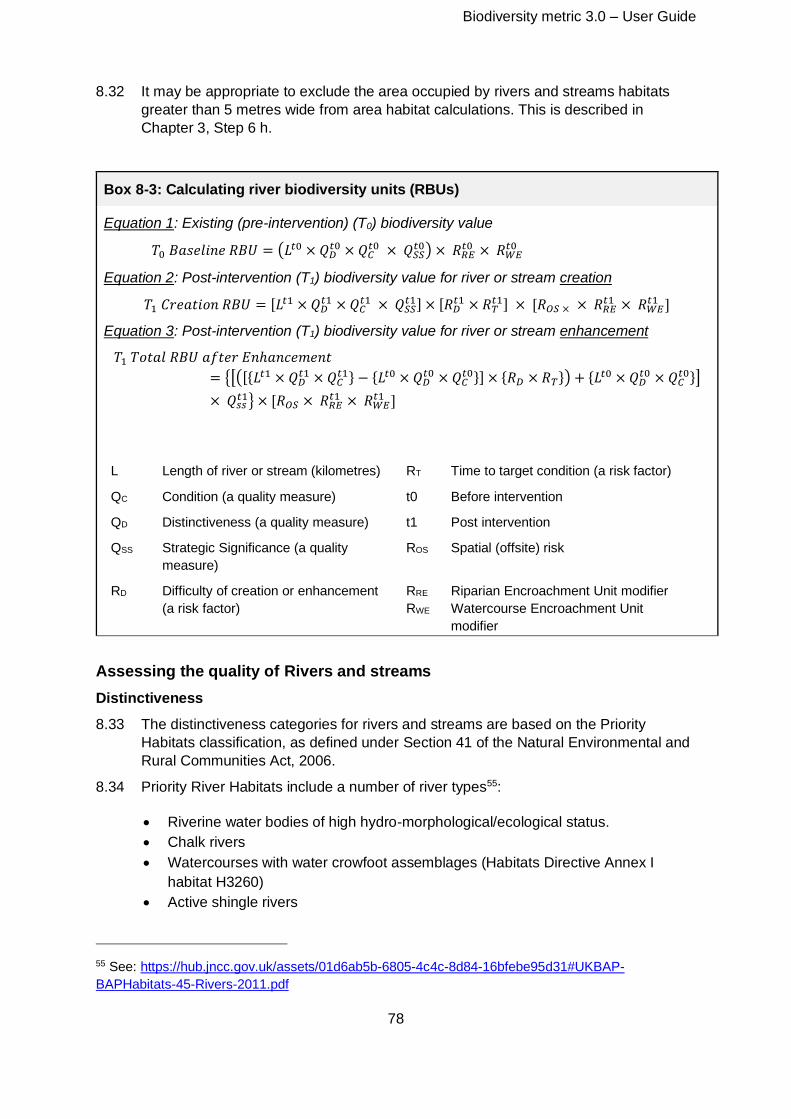
Biodiversity metric 3.0 – User Guide
78
8.32 It may be appropriate to exclude the area occupied by rivers and streams habitats
greater than 5 metres wide from area habitat calculations. This is described in
Chapter 3, Step 6 h.
Box 8-3: Calculating river biodiversity units (RBUs)
Equation 1: Existing (pre-intervention) (T0) biodiversity value
𝑇0 𝐵𝑎𝑠𝑒𝑙𝑖𝑛𝑒 𝑅𝐵𝑈 = (𝐿𝑡0 × 𝑄𝐷𝑡0 × 𝑄𝐶
𝑡0 × 𝑄𝑆𝑆𝑡0) × 𝑅𝑅𝐸
𝑡0 × 𝑅𝑊𝐸𝑡0
Equation 2: Post-intervention (T1) biodiversity value for river or stream creation
𝑇1 𝐶𝑟𝑒𝑎𝑡𝑖𝑜𝑛 𝑅𝐵𝑈 = [𝐿𝑡1 × 𝑄𝐷𝑡1 × 𝑄𝐶
𝑡1 × 𝑄𝑆𝑆𝑡1] × [𝑅𝐷
𝑡1 × 𝑅𝑇𝑡1] × [𝑅𝑂𝑆 × × 𝑅𝑅𝐸
𝑡1 × 𝑅𝑊𝐸𝑡1 ]
Equation 3: Post-intervention (T1) biodiversity value for river or stream enhancement
𝑇1 𝑇𝑜𝑡𝑎𝑙 𝑅𝐵𝑈 𝑎𝑓𝑡𝑒𝑟 𝐸𝑛ℎ𝑎𝑛𝑐𝑒𝑚𝑒𝑛𝑡
= {[([{𝐿𝑡1 × 𝑄𝐷𝑡1 × 𝑄𝐶
𝑡1} − {𝐿𝑡0 × 𝑄𝐷𝑡0 × 𝑄𝐶
𝑡0}] × {𝑅𝐷 × 𝑅𝑇}) + {𝐿𝑡0 × 𝑄𝐷𝑡0 × 𝑄𝐶
𝑡0}]
× 𝑄𝑠𝑠𝑡1} × [𝑅𝑂𝑆 × 𝑅𝑅𝐸
𝑡1 × 𝑅𝑊𝐸𝑡1 ]
L Length of river or stream (kilometres) RT Time to target condition (a risk factor)
QC Condition (a quality measure) t0 Before intervention
QD Distinctiveness (a quality measure) t1 Post intervention
QSS Strategic Significance (a quality
measure)
ROS Spatial (offsite) risk
RD Difficulty of creation or enhancement
(a risk factor)
RRE
RWE
Riparian Encroachment Unit modifier
Watercourse Encroachment Unit
modifier
Assessing the quality of Rivers and streams
Distinctiveness
8.33 The distinctiveness categories for rivers and streams are based on the Priority
Habitats classification, as defined under Section 41 of the Natural Environmental and
Rural Communities Act, 2006.
8.34 Priority River Habitats include a number of river types55:
• Riverine water bodies of high hydro-morphological/ecological status.
• Chalk rivers
• Watercourses with water crowfoot assemblages (Habitats Directive Annex I
habitat H3260)
• Active shingle rivers
55 See: https://hub.jncc.gov.uk/assets/01d6ab5b-6805-4c4c-8d84-16bfebe95d31#UKBAP-
BAPHabitats-45-Rivers-2011.pdf
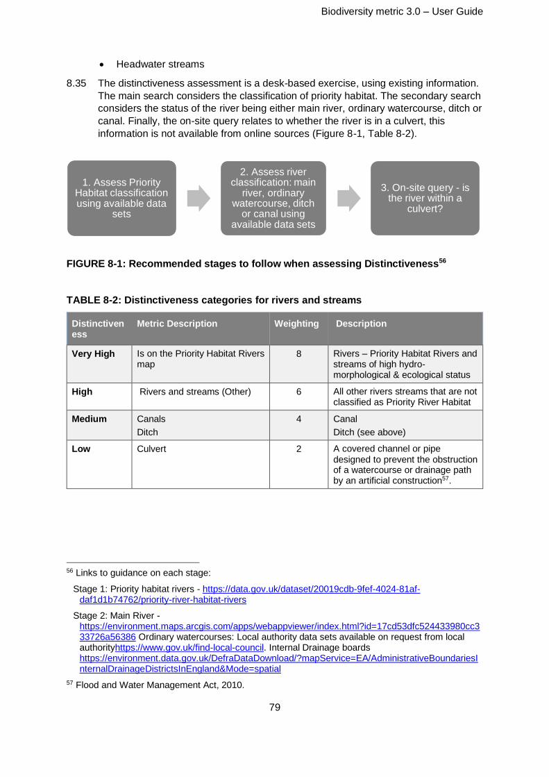
Biodiversity metric 3.0 – User Guide
79
• Headwater streams
8.35 The distinctiveness assessment is a desk-based exercise, using existing information.
The main search considers the classification of priority habitat. The secondary search
considers the status of the river being either main river, ordinary watercourse, ditch or
canal. Finally, the on-site query relates to whether the river is in a culvert, this
information is not available from online sources (Figure 8-1, Table 8-2).
FIGURE 8-1: Recommended stages to follow when assessing Distinctiveness56
TABLE 8-2: Distinctiveness categories for rivers and streams
Distinctiveness
Metric Description Weighting Description
Very High Is on the Priority Habitat Rivers map
8 Rivers – Priority Habitat Rivers and streams of high hydro-morphological & ecological status
High Rivers and streams (Other) 6 All other rivers streams that are not classified as Priority River Habitat
Medium Canals
Ditch
4 Canal
Ditch (see above)
Low Culvert 2 A covered channel or pipe designed to prevent the obstruction of a watercourse or drainage path by an artificial construction57.
56 Links to guidance on each stage:
Stage 1: Priority habitat rivers - https://data.gov.uk/dataset/20019cdb-9fef-4024-81af-daf1d1b74762/priority-river-habitat-rivers
Stage 2: Main River - https://environment.maps.arcgis.com/apps/webappviewer/index.html?id=17cd53dfc524433980cc333726a56386 Ordinary watercourses: Local authority data sets available on request from local authorityhttps://www.gov.uk/find-local-council. Internal Drainage boards https://environment.data.gov.uk/DefraDataDownload/?mapService=EA/AdministrativeBoundariesInternalDrainageDistrictsInEngland&Mode=spatial
57 Flood and Water Management Act, 2010.
1. Assess Priority Habitat classification using available data
sets
2. Assess river classification: main
river, ordinary watercourse, ditch
or canal using available data sets
3. On-site query - is the river within a
culvert?
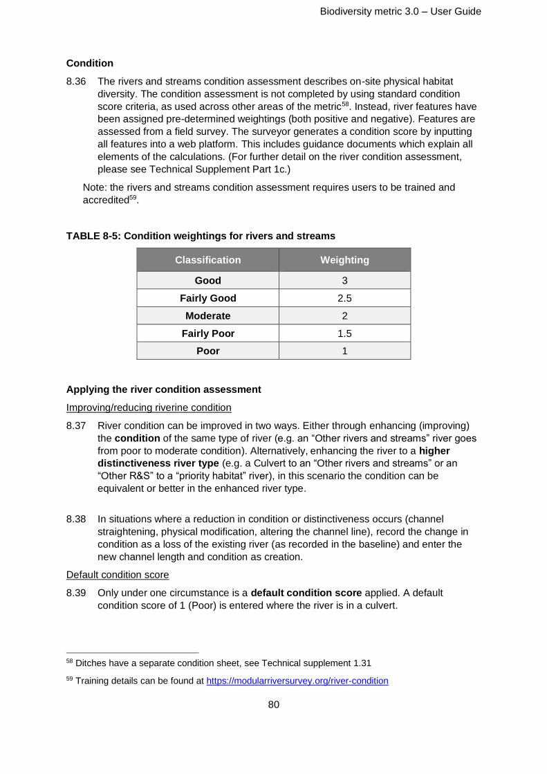
Biodiversity metric 3.0 – User Guide
80
Condition
8.36 The rivers and streams condition assessment describes on-site physical habitat
diversity. The condition assessment is not completed by using standard condition
score criteria, as used across other areas of the metric58. Instead, river features have
been assigned pre-determined weightings (both positive and negative). Features are
assessed from a field survey. The surveyor generates a condition score by inputting
all features into a web platform. This includes guidance documents which explain all
elements of the calculations. (For further detail on the river condition assessment,
please see Technical Supplement Part 1c.)
Note: the rivers and streams condition assessment requires users to be trained and
accredited59.
TABLE 8-5: Condition weightings for rivers and streams
Classification Weighting
Good 3
Fairly Good 2.5
Moderate 2
Fairly Poor 1.5
Poor 1
Applying the river condition assessment
Improving/reducing riverine condition
8.37 River condition can be improved in two ways. Either through enhancing (improving)
the condition of the same type of river (e.g. an “Other rivers and streams” river goes
from poor to moderate condition). Alternatively, enhancing the river to a higher
distinctiveness river type (e.g. a Culvert to an “Other rivers and streams” or an
“Other R&S” to a “priority habitat” river), in this scenario the condition can be
equivalent or better in the enhanced river type.
8.38 In situations where a reduction in condition or distinctiveness occurs (channel
straightening, physical modification, altering the channel line), record the change in
condition as a loss of the existing river (as recorded in the baseline) and enter the
new channel length and condition as creation.
Default condition score
8.39 Only under one circumstance is a default condition score applied. A default
condition score of 1 (Poor) is entered where the river is in a culvert.
58 Ditches have a separate condition sheet, see Technical supplement 1.31
59 Training details can be found at https://modularriversurvey.org/river-condition
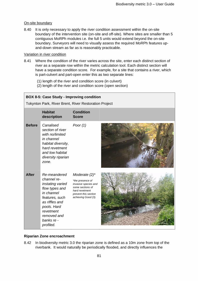
Biodiversity metric 3.0 – User Guide
81
On-site boundary
8.40 It is only necessary to apply the river condition assessment within the on-site
boundary of the intervention site (on-site and off-site). Where sites are smaller than 5
contiguous MoRPh modules i.e. the full 5 units would extend beyond the on-site
boundary. Surveyors will need to visually assess the required MoRPh features up-
and-down stream as far as is reasonably practicable.
Variation in river condition
8.41 Where the condition of the river varies across the site, enter each distinct section of
river as a separate row within the metric calculation tool. Each distinct section will
have a separate condition score. For example, for a site that contains a river, which
is part-culvert and part-open enter this as two separate lines:
(1) length of the river and condition score (in culvert)
(2) length of the river and condition score (open section)
BOX 8-5: Case Study - Improving condition
Tokynton Park, River Brent, River Restoration Project
Habitat
description
Condition
Score
Before Canalised
section of river
with no/limited
in channel
habitat diversity,
hard revetment
and low habitat
diversity riparian
zone.
Poor (1)
After Re-meandered
channel re-
instating varied
flow types and
in channel
features, such
as riffles and
pools. Hard
revetment
removed and
banks re -
profiled.
Moderate (2)*
*the presence of
invasive species and
some sections of
hard revetment
prevent this section
achieving Good (3).
Riparian Zone encroachment
8.42 In biodiversity metric 3.0 the riparian zone is defined as a 10m zone from top of the
riverbank. It would naturally be periodically flooded, and directly influences the
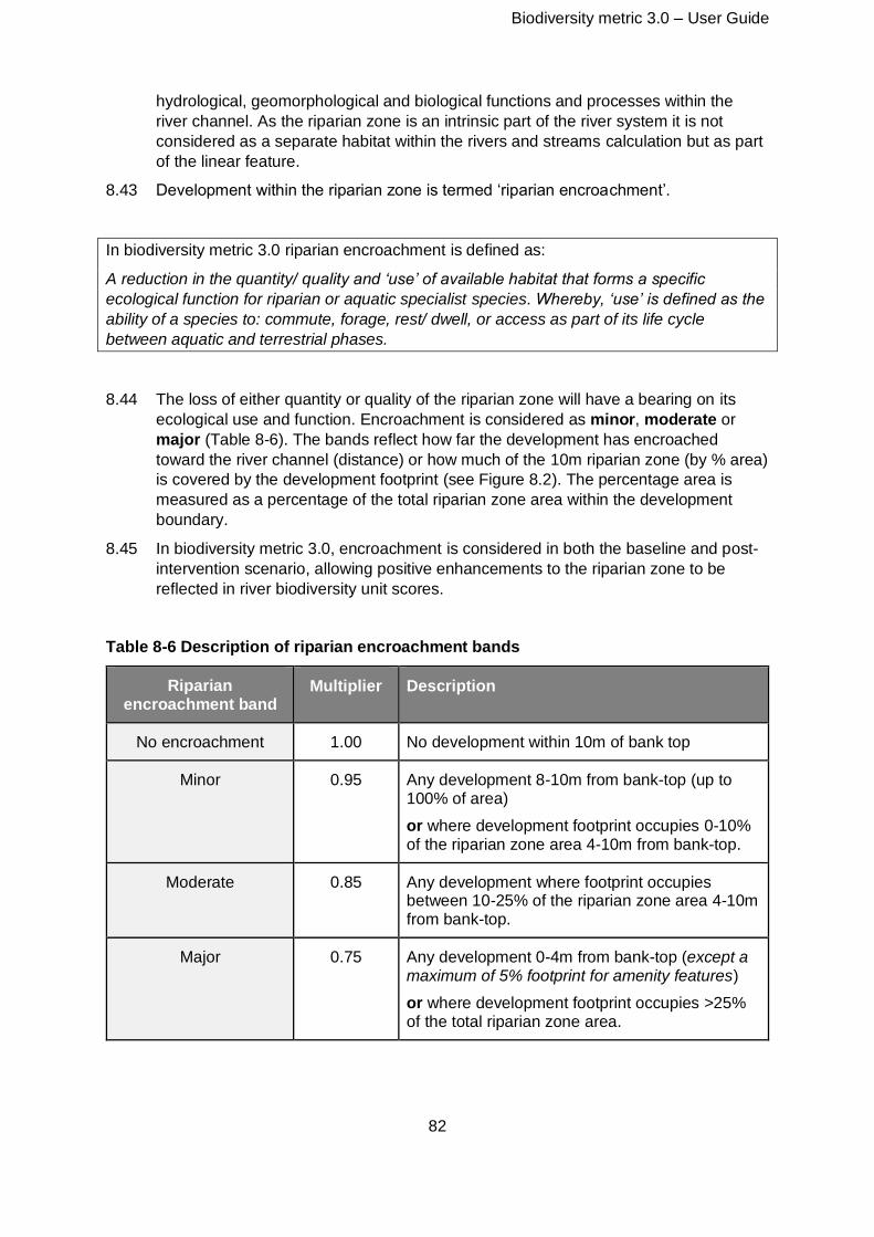
Biodiversity metric 3.0 – User Guide
82
hydrological, geomorphological and biological functions and processes within the
river channel. As the riparian zone is an intrinsic part of the river system it is not
considered as a separate habitat within the rivers and streams calculation but as part
of the linear feature.
8.43 Development within the riparian zone is termed ‘riparian encroachment’.
In biodiversity metric 3.0 riparian encroachment is defined as:
A reduction in the quantity/ quality and ‘use’ of available habitat that forms a specific
ecological function for riparian or aquatic specialist species. Whereby, ‘use’ is defined as the
ability of a species to: commute, forage, rest/ dwell, or access as part of its life cycle
between aquatic and terrestrial phases.
8.44 The loss of either quantity or quality of the riparian zone will have a bearing on its
ecological use and function. Encroachment is considered as minor, moderate or
major (Table 8-6). The bands reflect how far the development has encroached
toward the river channel (distance) or how much of the 10m riparian zone (by % area)
is covered by the development footprint (see Figure 8.2). The percentage area is
measured as a percentage of the total riparian zone area within the development
boundary.
8.45 In biodiversity metric 3.0, encroachment is considered in both the baseline and post-
intervention scenario, allowing positive enhancements to the riparian zone to be
reflected in river biodiversity unit scores.
Table 8-6 Description of riparian encroachment bands
Riparian encroachment band
Multiplier Description
No encroachment 1.00 No development within 10m of bank top
Minor 0.95 Any development 8-10m from bank-top (up to 100% of area)
or where development footprint occupies 0-10% of the riparian zone area 4-10m from bank-top.
Moderate 0.85 Any development where footprint occupies between 10-25% of the riparian zone area 4-10m from bank-top.
Major 0.75 Any development 0-4m from bank-top (except a maximum of 5% footprint for amenity features)
or where development footprint occupies >25% of the total riparian zone area.
Biodiversity metric 3.0 – User Guide
83
8.46 The riparian zone can be enhanced through reducing the extent of encroachment.
For example, by removing hard-standing or other structures, reconnecting channel–
riparian interactions. Beneficial measures such as providing appropriate planting that
improves riparian habitat complexity, installing green roofs/walls, and/or the inclusion
of wetland features such as backwaters and ponds can also be incorporated into the
riparian zone and contribute to generating in area biodiversity units (See 8.49 below).
8.47 If you need to offset losses which are caused by encroachment into the riparian zone,
then you are not restricted to delivering riparian betterment. Gains can also be
achieved through improvements to the condition of the river or reducing in-channel
encroachment. For example, removing toe boarding or installing in-channel woody
debris.
8.48 The riparian zone is an intrinsic part of the river system and is assessed within the
river condition assessment. To avoid double counting, river biodiversity units have
been designed to work alongside area biodiversity units in the riparian zone. The area
that the riparian zone occupies, and the habitats therein, are should also be recorded
in the area habitats tab of the metric calculator tool. For example, a stand of wet
woodland in the riparian zone that inputs large amounts of woody material into the
channel would be an important aspect of how the river functions and the in-channel
habitat features it generates but its area biodiversity unit value is also recorded in the
area habitats tab of the calculation tool.
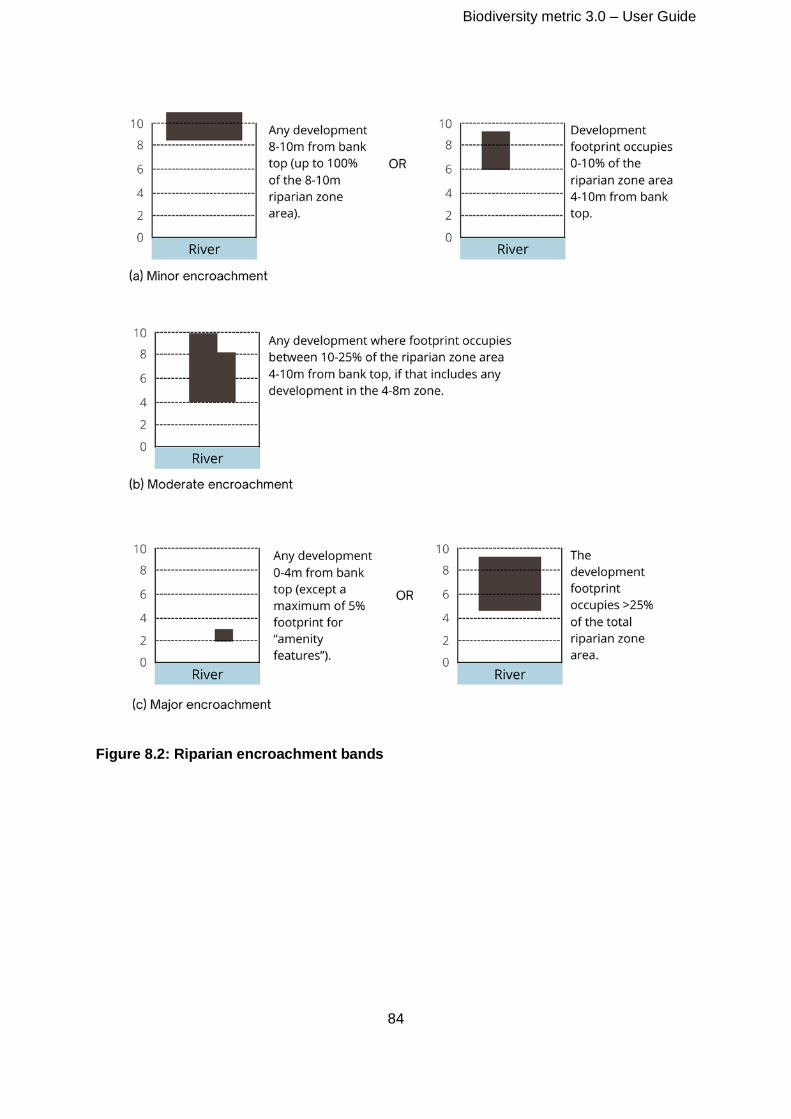
Biodiversity metric 3.0 – User Guide
84
Figure 8.2: Riparian encroachment bands
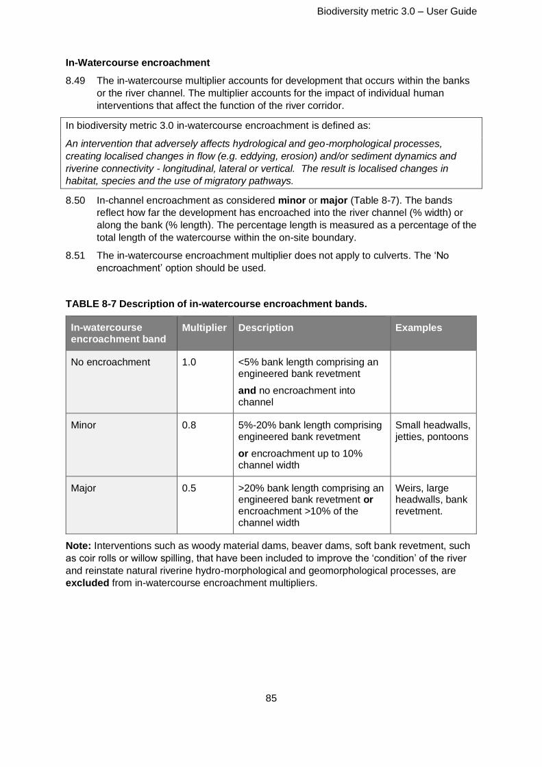
Biodiversity metric 3.0 – User Guide
85
In-Watercourse encroachment
8.49 The in-watercourse multiplier accounts for development that occurs within the banks
or the river channel. The multiplier accounts for the impact of individual human
interventions that affect the function of the river corridor.
In biodiversity metric 3.0 in-watercourse encroachment is defined as:
An intervention that adversely affects hydrological and geo-morphological processes,
creating localised changes in flow (e.g. eddying, erosion) and/or sediment dynamics and
riverine connectivity - longitudinal, lateral or vertical. The result is localised changes in
habitat, species and the use of migratory pathways.
8.50 In-channel encroachment as considered minor or major (Table 8-7). The bands
reflect how far the development has encroached into the river channel (% width) or
along the bank (% length). The percentage length is measured as a percentage of the
total length of the watercourse within the on-site boundary.
8.51 The in-watercourse encroachment multiplier does not apply to culverts. The ‘No
encroachment’ option should be used.
TABLE 8-7 Description of in-watercourse encroachment bands.
In-watercourse encroachment band
Multiplier Description Examples
No encroachment 1.0 <5% bank length comprising an engineered bank revetment
and no encroachment into channel
Minor 0.8 5%-20% bank length comprising engineered bank revetment
or encroachment up to 10% channel width
Small headwalls, jetties, pontoons
Major 0.5 >20% bank length comprising an engineered bank revetment or encroachment >10% of the channel width
Weirs, large headwalls, bank revetment.
Note: Interventions such as woody material dams, beaver dams, soft bank revetment, such
as coir rolls or willow spilling, that have been included to improve the ‘condition’ of the river
and reinstate natural riverine hydro-morphological and geomorphological processes, are
excluded from in-watercourse encroachment multipliers.
Biodiversity metric 3.0 – User Guide
86
Strategic significance
8.52 The purpose of the Strategic significance multiplier is outlined in Chapter 5. For
Rivers and streams we use the delivery of identified actions within River Basin
Management Plans, Catchment Plans and Local Plans to represent high strategic
significance.
TABLE 8-8: Strategic significance multipliers for rivers and streams
Description of multiplier Strategic multiplier
High Delivery of River restoration actions within:
• Local Plans
• River Basin Management Plan
• Catchment Plans
• Catchment Planning System
• Priority Habitats for Restoration60
1.15
Low Low potential/ action not identified in any plan.
1
Risks
Difficulty of creation and enhancement of rivers and streams
8.53 Rivers, by their nature, cannot be created. However, there can be circumstances
where new artificial river channels are ‘created’. In most instances, rivers will be
enhanced through positive management and restoration.
8.54 Where new, engineered watercourses are created the difficulty of creation is high due
to the complexity of the work. For culverts, canals and ditches difficulty of creation is
low. Enhancement difficulty is defined as medium for all rivers and streams habitat
types (See Table 8-10).
8.55 In Biodiversity metric 3.0 creation and enhancement for rivers and streams are
defined in Table 8-9.
60 Contact the local catchment partnership for information. Contribute restoration priorities data –
Discovering Priority Habitats in England
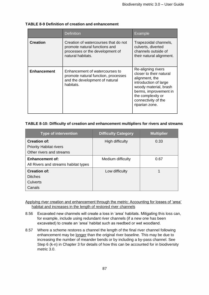
Biodiversity metric 3.0 – User Guide
87
TABLE 8-9 Definition of creation and enhancement
Definition Example
Creation Creation of watercourses that do not promote natural functions and processes or the development of natural habitats.
Trapezoidal channels, culverts, diverted channels outside of their natural alignment.
Enhancement Enhancement of watercourses to promote natural function, processes and the development of natural habitats.
Re-aligning rivers closer to their natural alignment, the introduction of large woody material, brash berms, improvement in the complexity or connectivity of the riparian zone.
TABLE 8-10: Difficulty of creation and enhancement multipliers for rivers and streams
Type of intervention Difficulty Category Multiplier
Creation of:
Priority Habitat rivers
Other rivers and streams
High difficulty 0.33
Enhancement of:
All Rivers and streams habitat types
Medium difficulty 0.67
Creation of:
Ditches
Culverts
Canals
Low difficulty 1
Applying river creation and enhancement through the metric: Accounting for losses of ‘area’
habitat and increases in the length of restored river channels
8.56 Excavated new channels will create a loss in ‘area’ habitats. Mitigating this loss can,
for example, include using redundant river channels (if a new one has been
excavated) to create an ‘area’ habitat such as reedbed or wet woodland.
8.57 Where a scheme restores a channel the length of the final river channel following
enhancement may be longer than the original river baseline. This may be due to
increasing the number of meander bends or by including a by-pass channel. See
Step 6 (k-n) in Chapter 3 for details of how this can be accounted for in biodiversity
metric 3.0.
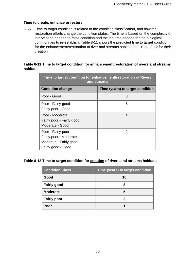
Biodiversity metric 3.0 – User Guide
88
Time to create, enhance or restore
8.58 Time to target condition is related to the condition classification, and how far
restoration efforts change the condition status. The time is based on the complexity of
intervention needed to raise condition and the lag time needed for the biological
communities to re-establish. Table 8-11 shows the predicted time to target condition
for the enhancement/restoration of river and streams habitats and Table 8-12 for their
creation.
Table 8-11 Time to target condition for enhancement/restoration of rivers and streams
habitats
Time to target condition for enhancement/restoration of Rivers and streams
Condition change Time (years) to target condition
Poor - Good 8
Poor - Fairly good
Fairly poor - Good
6
Poor - Moderate
Fairly poor - Fairly good
Moderate - Good
4
Poor - Fairly poor
Fairly poor - Moderate
Moderate - Fairly good
Fairly good - Good
2
Table 8-12 Time to target condition for creation of rivers and streams habitats
Condition Class Time (years) to target condition
Good 10
Fairly good 8
Moderate 5
Fairly poor 2
Poor 1
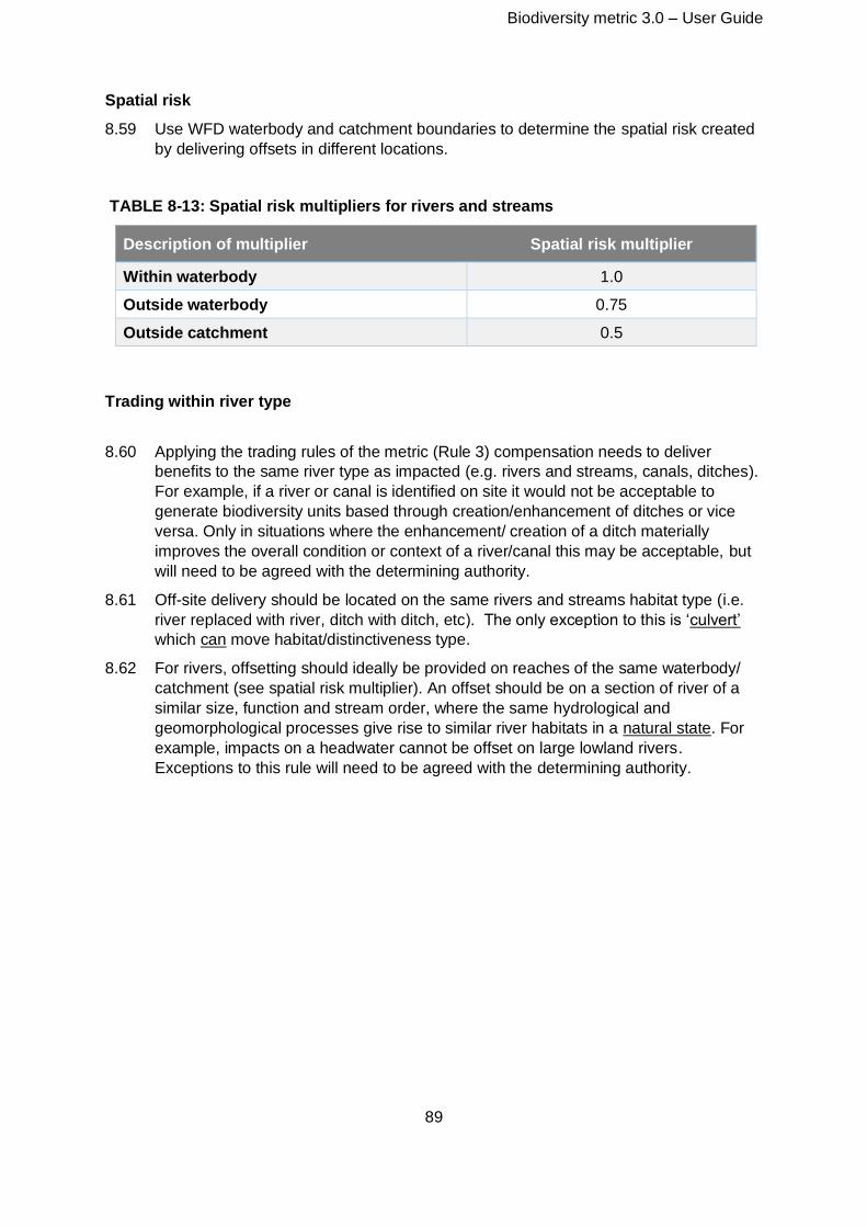
Biodiversity metric 3.0 – User Guide
89
Spatial risk
8.59 Use WFD waterbody and catchment boundaries to determine the spatial risk created
by delivering offsets in different locations.
TABLE 8-13: Spatial risk multipliers for rivers and streams
Description of multiplier Spatial risk multiplier
Within waterbody 1.0
Outside waterbody 0.75
Outside catchment 0.5
Trading within river type
8.60 Applying the trading rules of the metric (Rule 3) compensation needs to deliver
benefits to the same river type as impacted (e.g. rivers and streams, canals, ditches).
For example, if a river or canal is identified on site it would not be acceptable to
generate biodiversity units based through creation/enhancement of ditches or vice
versa. Only in situations where the enhancement/ creation of a ditch materially
improves the overall condition or context of a river/canal this may be acceptable, but
will need to be agreed with the determining authority.
8.61 Off-site delivery should be located on the same rivers and streams habitat type (i.e.
river replaced with river, ditch with ditch, etc). The only exception to this is ‘culvert’
which can move habitat/distinctiveness type.
8.62 For rivers, offsetting should ideally be provided on reaches of the same waterbody/
catchment (see spatial risk multiplier). An offset should be on a section of river of a
similar size, function and stream order, where the same hydrological and
geomorphological processes give rise to similar river habitats in a natural state. For
example, impacts on a headwater cannot be offset on large lowland rivers.
Exceptions to this rule will need to be agreed with the determining authority.
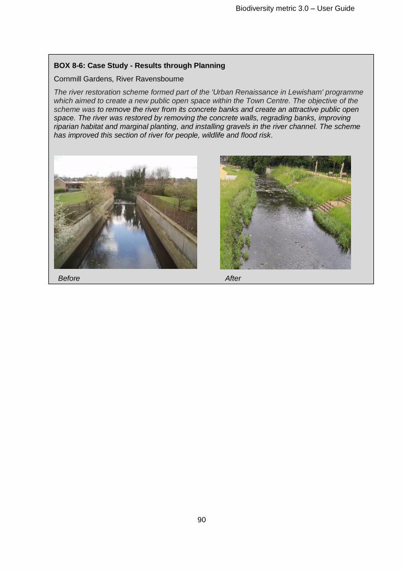
Biodiversity metric 3.0 – User Guide
90
BOX 8-6: Case Study - Results through Planning
Cornmill Gardens, River Ravensbourne
The river restoration scheme formed part of the 'Urban Renaissance in Lewisham' programme which aimed to create a new public open space within the Town Centre. The objective of the scheme was to remove the river from its concrete banks and create an attractive public open space. The river was restored by removing the concrete walls, regrading banks, improving riparian habitat and marginal planting, and installing gravels in the river channel. The scheme has improved this section of river for people, wildlife and flood risk.
Before After
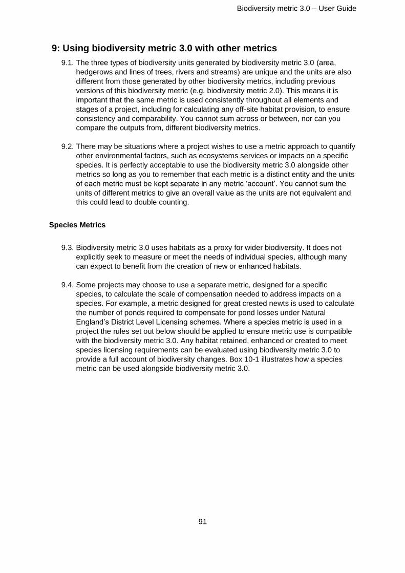
Biodiversity metric 3.0 – User Guide
91
9: Using biodiversity metric 3.0 with other metrics
9.1. The three types of biodiversity units generated by biodiversity metric 3.0 (area,
hedgerows and lines of trees, rivers and streams) are unique and the units are also
different from those generated by other biodiversity metrics, including previous
versions of this biodiversity metric (e.g. biodiversity metric 2.0). This means it is
important that the same metric is used consistently throughout all elements and
stages of a project, including for calculating any off-site habitat provision, to ensure
consistency and comparability. You cannot sum across or between, nor can you
compare the outputs from, different biodiversity metrics.
9.2. There may be situations where a project wishes to use a metric approach to quantify
other environmental factors, such as ecosystems services or impacts on a specific
species. It is perfectly acceptable to use the biodiversity metric 3.0 alongside other
metrics so long as you to remember that each metric is a distinct entity and the units
of each metric must be kept separate in any metric ‘account’. You cannot sum the
units of different metrics to give an overall value as the units are not equivalent and
this could lead to double counting.
Species Metrics
9.3. Biodiversity metric 3.0 uses habitats as a proxy for wider biodiversity. It does not
explicitly seek to measure or meet the needs of individual species, although many
can expect to benefit from the creation of new or enhanced habitats.
9.4. Some projects may choose to use a separate metric, designed for a specific
species, to calculate the scale of compensation needed to address impacts on a
species. For example, a metric designed for great crested newts is used to calculate
the number of ponds required to compensate for pond losses under Natural
England’s District Level Licensing schemes. Where a species metric is used in a
project the rules set out below should be applied to ensure metric use is compatible
with the biodiversity metric 3.0. Any habitat retained, enhanced or created to meet
species licensing requirements can be evaluated using biodiversity metric 3.0 to
provide a full account of biodiversity changes. Box 10-1 illustrates how a species
metric can be used alongside biodiversity metric 3.0.
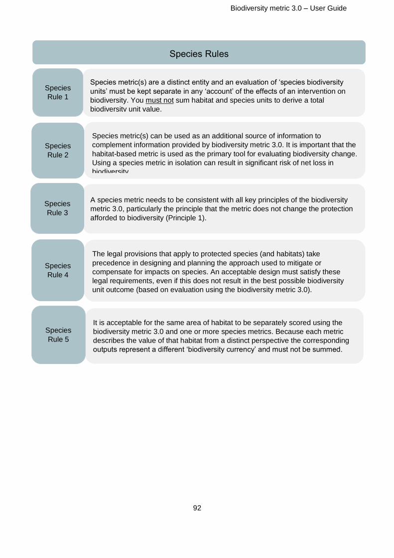
Biodiversity metric 3.0 – User Guide
92
Species metric(s) are a distinct entity and an evaluation of ‘species biodiversity
units’ must be kept separate in any ‘account’ of the effects of an intervention on
biodiversity. You must not sum habitat and species units to derive a total
biodiversity unit value.
Species
Rule 1
Species Rules
Species metric(s) can be used as an additional source of information to
complement information provided by biodiversity metric 3.0. It is important that the
habitat-based metric is used as the primary tool for evaluating biodiversity change.
Using a species metric in isolation can result in significant risk of net loss in
biodiversity.
Species
Rule 2
A species metric needs to be consistent with all key principles of the biodiversity
metric 3.0, particularly the principle that the metric does not change the protection
afforded to biodiversity (Principle 1).
Species
Rule 3
The legal provisions that apply to protected species (and habitats) take
precedence in designing and planning the approach used to mitigate or
compensate for impacts on species. An acceptable design must satisfy these
legal requirements, even if this does not result in the best possible biodiversity
unit outcome (based on evaluation using the biodiversity metric 3.0).
Species
Rule 4
It is acceptable for the same area of habitat to be separately scored using the
biodiversity metric 3.0 and one or more species metrics. Because each metric
describes the value of that habitat from a distinct perspective the corresponding
outputs represent a different ‘biodiversity currency’ and must not be summed.
Species
Rule 5
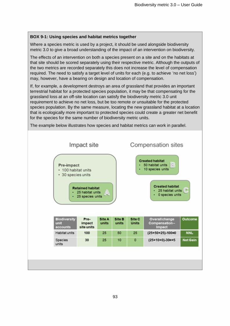
Biodiversity metric 3.0 – User Guide
93
BOX 9-1: Using species and habitat metrics together
Where a species metric is used by a project, it should be used alongside biodiversity
metric 3.0 to give a broad understanding of the impact of an intervention on biodiversity.
The effects of an intervention on both a species present on a site and on the habitats at
that site should be scored separately using their respective metric. Although the outputs of
the two metrics are recorded separately this does not increase the level of compensation
required. The need to satisfy a target level of units for each (e.g. to achieve ‘no net loss’)
may, however, have a bearing on design and location of compensation.
If, for example, a development destroys an area of grassland that provides an important
terrestrial habitat for a protected species population, it may be that compensating for the
grassland loss at an off-site location can satisfy the biodiversity metric 3.0 unit
requirement to achieve no net loss, but be too remote or unsuitable for the protected
species population. By the same measure, locating the new grassland habitat at a location
that is ecologically more important to protected species could create a greater net benefit
for the species for the same number of biodiversity metric units.
The example below illustrates how species and habitat metrics can work in parallel.
Biodiversity metric 3.0 – User Guide
94
References
BAKER, J, SHEATE, W.R., BENNETT, T., PAYNE, D., TUCKER, G. WHITE, O AND
FORREST, S. 2014. Evaluation of the Biodiversity Offsetting Pilot Programme. Final Report.
Defra project code: WC 1051. Collingwood Environmental Planning Limited, London, UK
BBOP, 2012, Standard on biodiversity offsets. Business and Biodiversity Offsets Programme
(BBOP). Forest Trends, Washington, DC. http://www.forest-
trends.org/documents/files/doc_3078.pdf
BBOP, 2012a, Glossary with updates. Business and Biodiversity Offsets Programme
(BBOP). Forest Trends, Washington, DC. Available from http://bbop.forest-
trends.org/guidelines/Updated_Glossary
CIEEM, CIRIA, IEMA. 2016 Biodiversity Net Gain – Good Practice Principles For
Development.
https://www.cieem.net/data/files/Publications/Biodiversity_Net_Gain_Principles.pdf
CONSERVATION SERVICE. 2007. Guidelines for regenerating derelict hedgerows. Peak
District National Park Authority.
http://www.peakdistrict.gov.uk/__data/assets/pdf_file/0003/78861/derelict-hedgerows.pdf
CONVENTION ON BIOLOGICAL DIVERSITY,
https://www.cbd.int/convention/articles/default.shtml?a=cbd-02 (Accessed 19/06/2019)
DEFRA. 2007. Hedgerow Survey Handbook. A standard procedure for local surveys in the
UK. Defra, London. PB1195.
https://www.gov.uk/government/uploads/system/uploads/attachment_data/file/69285/pb1195
1-hedgerow-survey-handbook-070314.pdf
DEFRA. 2012. Biodiversity offsetting pilots. Technical paper: the metric for the biodiversity
offsetting pilot in England. Defra. March 2012.
https://www.gov.uk/government/collections/biodiversity-offsetting (Accessed 16-6-17)
DEFRA, 2018, Net Gain Consultation Proposals. Defra, December 2018
https://consult.defra.gov.uk/land-use/net-
gain/supporting_documents/netgainconsultationdocument.pdf
FOULKES, N., FULLER, J., LITTLE, D., MCCOURT, S., & MURPHY, P. 2013. Hedgerow
Appraisal System – best practice guidance on hedgerow survey, data collation and
appraisal. Woodlands of Ireland, Dublin.
ENGLAND AND GURNELL, 2016. England, J. and Gurnell, A.M. (2016) Incorporating
Catchment to Reach Scale Processes into Hydromorphology Assessment in the UK. Water
and Environment Journal, 30: 22–30.
GURNELL, A.M., ENGLAND, J., SHUKER, L., WHARTON, G. (in review). The contribution
of citizen science volunteers to river monitoring and management: International and national
perspectives and the example of the MoRPh survey.
Biodiversity metric 3.0 – User Guide
95
GURNELL, A.M., RINALDI, M., BELLETTI, B., BIZZI, S., BLAMAUER, B., BRACA, G.,
BUIJSE, T., BUSSETTINI, M., CAMENEN, B., COMITI, F., DEMARCHI, L., GARCÍA DE
JALÓN, D., GONZÁLEZ DEL TÁNAGO, M., GRABOWSKI, R.C., GUNN, I.D.M.,
HABERSACK, H., HENDRIKS, D., HENSHAW, A.J., KLÖSCH, M., LASTORIA, B.,
LATAPIE, A., MARCINKOWSKI, P., MARTÍNEZ-FERNÁNDEZ, V., MOSSELMAN, E.,
MOUNTFORD, J.O., NARDI, L., OKRUSZKO, T., O’HARE, M.T., PALMA, M., PERCOPO,
C., SURIAN, N., VAN DE BUND, W., WEISSTEINER, C. AND ZILIANI, L., 2016. A multi-
scale hierarchical framework for developing understanding of river behaviour to support river
management. Aquatic Sciences, 78(1): 1-16.
HM TREASURY. 2011. The Green Book: Appraisal and Evaluation in Central Government,
TSO, London.
HODGE. SJ. 1991. Urban trees: a Survey of street trees in Britain. Forestry Commission
Bulletin 99. HMSO, London. Available from:
https://www.forestresearch.gov.uk/research/archive-urban-trees-a-survey-of-street-trees-in-
britain/ (Accessed 21/06/2019)
HOUSES OF PARLIAMENT, 2014, Ancient Woodland. POSTNOTE Number 465 June
2014. Parliamentary Office for Science and Technology.
http://www.parliament.uk/documents/POST/postpn465_Ancient-Woodlandreferences.pdf
IUCN 2015. No Net Loss and Net Positive Impact Approaches for Biodiversity Exploring the
potential application of these approaches in the commercial agriculture and forestry sectors.
http://cmsdata.iucn.org/downloads/npi_for_agriculture_and_forestry___overview_april_2015
_1.pdf
IUCN, 2016. IUCN Policy on Biodiversity Offsets – January 29, 2016
http://cmsdata.iucn.org/downloads/iucn_biodiversity_offsets_policy_jan_29_2016.pdf
(Accessed 15-6-16)
JNCC (2010) Handbook for Phase 1 habitat survey - a technique for environmental audit
(revised 2010)
KUJULA, H., WHITEHEAD, A.L., MORRIS, W.K., & WINTLE, B.A., 2015.Towards strategic
offsetting of biodiversity loss using spatial prioritization concepts and tools: a case study of
mining impacts in Australia. Biological Conservation 192 pp513-521.
LAWTON J.H., BROTHERTON P.N.M., BROWN V.K., ELPHICK C., FITTER A.H.,
FORSHAW J., HADDOW R.W., HILBORNE S., LEAFE R.N., MACE G.M., SOUTHGATE
M.P., SUTHERLAND W.J., TEW T.E., VARLEY J. & WYNEE G.R. (2010) Making Space for
Nature: a review of England's wildlife sites and ecological network. Report to Defra
RINALDI, M., GURNELL, A.M., GONZÁLEZ DEL TÁNAGO, M., BUSSETTINI, M. AND
HENDRIKS, D. 2016. Classification of river morphology and hydrology to support
management and restoration. Aquatic Sciences, 78(1): 17-33.
SHUKER, L.J., GURNELL, A.M., WHARTON, G., GURNELL, D.J., ENGLAND, J., FINN
LEEMING, B. AND BEACH, E. 2017. MoRPh: a citizen science tool for monitoring and
appraising physical habitat changes in rivers. Water and Environment Journal, 31(3): 418-
424.
Biodiversity metric 3.0 – User Guide
96
TAYLOR, S., KNIGHT, M. & HARFOOT, A., (2014) National biodiversity climate change
vulnerability model. Natural England Research Report NERR054. Natural England. ISBN
978-1-78354-084-6.
UKHAB WORKING GROUP (2018) UK Habitat Classification Documents.
http://ecountability.co.uk/ukhabworkinggroup-ukhab/ (Accessed 23 August 2018)
WALKER, M.P., DOVER, J.W., HINSLEY, S.A. & SPARKS, TH. 2005. Birds and green
lanes: Breeding season bird abundance, territories and species richness. Biological
Conservation, 126: 540–547.
WALKER, M.P., DOVER, J.W., SPARKS, T.H. & HINSLEY, S.A. 2006. Hedges and green
lanes: vegetation composition and structure. Biodiversity and Conservation, 15:2595–2610
WOLTON, R (2012) When is a hedge in Good condition for wildlife?
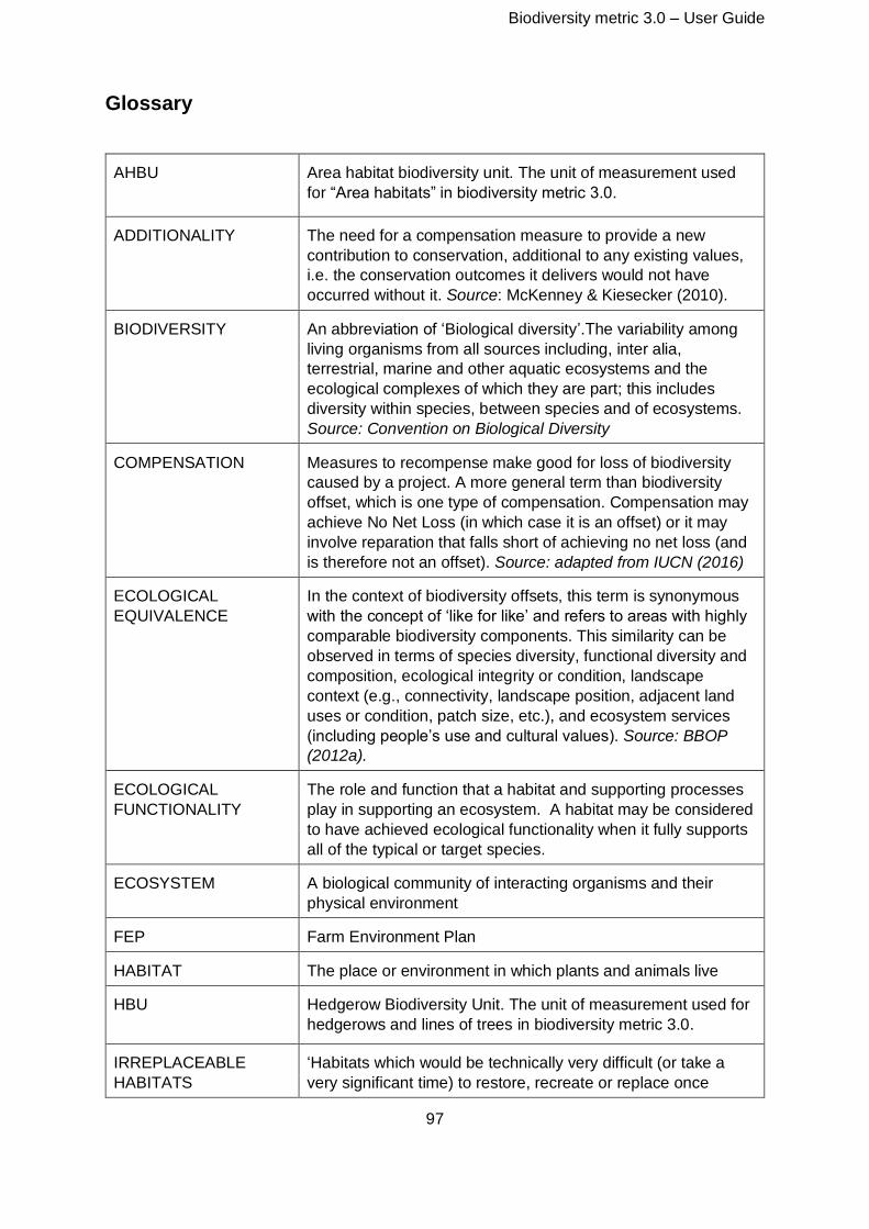
Biodiversity metric 3.0 – User Guide
97
Glossary
AHBU
Area habitat biodiversity unit. The unit of measurement used
for “Area habitats” in biodiversity metric 3.0.
ADDITIONALITY The need for a compensation measure to provide a new
contribution to conservation, additional to any existing values,
i.e. the conservation outcomes it delivers would not have
occurred without it. Source: McKenney & Kiesecker (2010).
BIODIVERSITY An abbreviation of ‘Biological diversity’.The variability among
living organisms from all sources including, inter alia,
terrestrial, marine and other aquatic ecosystems and the
ecological complexes of which they are part; this includes
diversity within species, between species and of ecosystems.
Source: Convention on Biological Diversity
COMPENSATION Measures to recompense make good for loss of biodiversity
caused by a project. A more general term than biodiversity
offset, which is one type of compensation. Compensation may
achieve No Net Loss (in which case it is an offset) or it may
involve reparation that falls short of achieving no net loss (and
is therefore not an offset). Source: adapted from IUCN (2016)
ECOLOGICAL
EQUIVALENCE
In the context of biodiversity offsets, this term is synonymous
with the concept of ‘like for like’ and refers to areas with highly
comparable biodiversity components. This similarity can be
observed in terms of species diversity, functional diversity and
composition, ecological integrity or condition, landscape
context (e.g., connectivity, landscape position, adjacent land
uses or condition, patch size, etc.), and ecosystem services
(including people’s use and cultural values). Source: BBOP
(2012a).
ECOLOGICAL
FUNCTIONALITY
The role and function that a habitat and supporting processes
play in supporting an ecosystem. A habitat may be considered
to have achieved ecological functionality when it fully supports
all of the typical or target species.
ECOSYSTEM A biological community of interacting organisms and their
physical environment
FEP Farm Environment Plan
HABITAT The place or environment in which plants and animals live
HBU Hedgerow Biodiversity Unit. The unit of measurement used for
hedgerows and lines of trees in biodiversity metric 3.0.
IRREPLACEABLE
HABITATS
‘Habitats which would be technically very difficult (or take a
very significant time) to restore, recreate or replace once
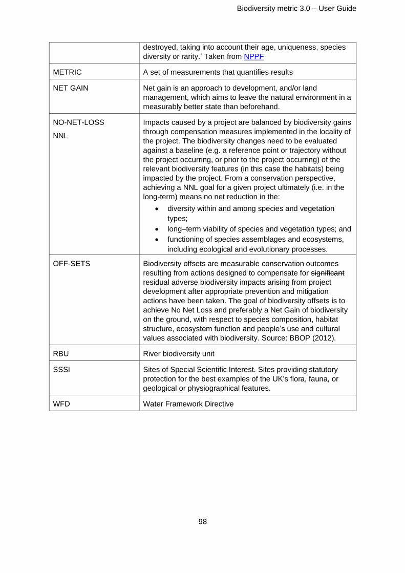
Biodiversity metric 3.0 – User Guide
98
destroyed, taking into account their age, uniqueness, species
diversity or rarity.’ Taken from NPPF
METRIC A set of measurements that quantifies results
NET GAIN Net gain is an approach to development, and/or land
management, which aims to leave the natural environment in a
measurably better state than beforehand.
NO-NET-LOSS
NNL
Impacts caused by a project are balanced by biodiversity gains
through compensation measures implemented in the locality of
the project. The biodiversity changes need to be evaluated
against a baseline (e.g. a reference point or trajectory without
the project occurring, or prior to the project occurring) of the
relevant biodiversity features (in this case the habitats) being
impacted by the project. From a conservation perspective,
achieving a NNL goal for a given project ultimately (i.e. in the
long-term) means no net reduction in the:
• diversity within and among species and vegetation
types;
• long–term viability of species and vegetation types; and
• functioning of species assemblages and ecosystems,
including ecological and evolutionary processes.
OFF-SETS Biodiversity offsets are measurable conservation outcomes
resulting from actions designed to compensate for significant
residual adverse biodiversity impacts arising from project
development after appropriate prevention and mitigation
actions have been taken. The goal of biodiversity offsets is to
achieve No Net Loss and preferably a Net Gain of biodiversity
on the ground, with respect to species composition, habitat
structure, ecosystem function and people’s use and cultural
values associated with biodiversity. Source: BBOP (2012).
RBU River biodiversity unit
SSSI Sites of Special Scientific Interest. Sites providing statutory
protection for the best examples of the UK's flora, fauna, or
geological or physiographical features.
WFD Water Framework Directive


![6 3 biodiversity[1]](https://img.pdfslide.net/doc/110x75/5461d293af79592e408b825f/6-3-biodiversity1.jpg)