BIOGAS PROCESSING Final Report

Prepared for

THE NEW YORK STATE ENERGY RESEARCH AND DEVELOPMENT AUTHORITY

Albany, New York

Tom Fiesinger Project Manager

Prepared by

New York State Electric & Gas Corporation Binghamton, New York

Bruce D. Roloson

Project Principal Investigator

And

Cornell University Ithaca, New York

Norman R. Scott

Co-principal Investigator

Kimberly Bothi Kelly Saikkonen

Steven Zicari

Agreement No. 7250 NYSERDA 7250 February 2006

NOTICE

This report was prepared by Cornell University for New York State Electric & Gas Corporation in the

course of performing work contracted for and sponsored by the New York State Energy Research and

Development Authority (hereafter “NYSERDA”). The opinions expressed in this report do not necessarily

reflect those of NYSERDA or the State of New York, and reference to any specific product, service,

process, or method does not constitute an implied or expressed recommendation or endorsement of it.

Further, NYSERDA, the State of New York, and the contractor make no warranties or representations,

expressed or implied, as to the fitness for particular purpose or merchantability of any product, apparatus,

or service, or the usefulness, completeness, or accuracy of any processes, methods, or other information

contained, described, disclosed, or referred to in this report. NYSERDA, the State of New York, and the

contractor make no representation that the use of any product, apparatus, process, method, or other

information will not infringe privately owned rights and will assume no liability for any loss, injury, or

damage resulting from, or occurring in connection with, the use of information contained, described,

disclosed, or referred to in this report.

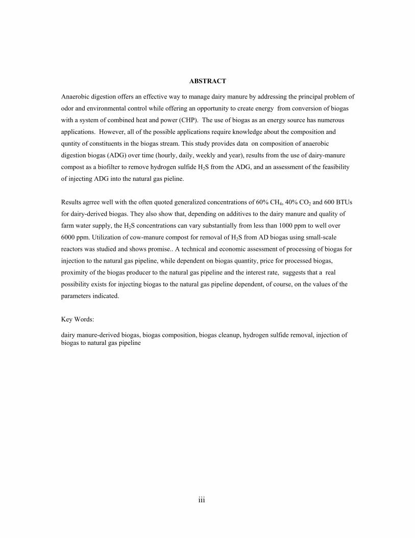
ABSTRACT Anaerobic digestion offers an effective way to manage dairy manure by addressing the principal problem of

odor and environmental control while offering an opportunity to create energy from conversion of biogas

with a system of combined heat and power (CHP). The use of biogas as an energy source has numerous

applications. However, all of the possible applications require knowledge about the composition and

quntity of constituents in the biogas stream. This study provides data on composition of anaerobic

digestion biogas (ADG) over time (hourly, daily, weekly and year), results from the use of dairy-manure

compost as a biofilter to remove hydrogen sulfide H2S from the ADG, and an assessment of the feasibility

of injecting ADG into the natural gas pieline.

Results agrree well with the often quoted generalized concentrations of 60% CH4, 40% CO2 and 600 BTUs

for dairy-derived biogas. They also show that, depending on additives to the dairy manure and quality of

farm water supply, the H2S concentrations can vary substantially from less than 1000 ppm to well over

6000 ppm. Utilization of cow-manure compost for removal of H2S from AD biogas using small-scale

reactors was studied and shows promise.. A technical and economic assessment of processing of biogas for

injection to the natural gas pipeline, while dependent on biogas quantity, price for processed biogas,

proximity of the biogas producer to the natural gas pipeline and the interest rate, suggests that a real

possibility exists for injecting biogas to the natural gas pipeline dependent, of course, on the values of the

parameters indicated.

Key Words: dairy manure-derived biogas, biogas composition, biogas cleanup, hydrogen sulfide removal, injection of biogas to natural gas pipeline

iii

ACKNOWLEDGEMENTS

Major specific results in this report represent the work of three Masters of Science students in the

Department of Biological and Environmental Engineering at Cornell University: Kimberly Bothi, Kelly

Saikkonen and Steven Zicari. An undergraduate student, Michelle Wright, provided much assistance.

Five participating dairies, used for data acquisition, are acknowledged for their important contributions:

Dairy Development International (DDI), AA Dairy, Matlink, Noblehurst, and Twin Birch. Special thanks

go to DDI, particularly Larry Jones, who provided the opportunity to acquire “real data” with on-site

experimentation.

iv

TABLE OF CONTENTS

Section Page SUMMARY ................................................................................................................................................ S-1 1. ................................................................................................................................... 1-1INTRODUCTION ........................................................................................................................... 1-2SCOPE OF PROJECT ................................................................................................................................... 1-2BACKGROUND ............................................................................................. 1-5FARM PARTICIPANT INFORMATION 2. BIOGAS CHARACTERIZATION......................................................................................................... 2-1 SAMPLING TECHNIQUES ................................................................................................................. 2-1 Biogas Bag Samples ......................................................................................................................... 2-1 Manure.............................................................................................................................................. 2-2 Water ................................................................................................................................................ 2-3 Forage ............................................................................................................................................... 2-3 ANALYTICAL TECHNIQUES............................................................................................................ 2-3

Determination of H 2S in biogas ........................................................................................................ 2-3 Manure Water Forage Samples......................................................................................................... 2-4 RESULTS FROM BIOGAS COLLECTION AND ANALYSIS .......................................................... 2-4 MANURE, WATER, AND FORAGE ANALYSES........................................................................... 2-10 3. BIOGAS PROCESSING......................................................................................................................... 3-1 “IRON SPONGE” RESULTS................................................................................................................ 3-4 4. ECONOMIC ASSESSMENT OF DAIRY-DERIVED BIOGAS INJECTION INTO NATURAL GAS

PIPELINE .............................................................................................................................................. 4-1 Background ........................................................................................................................................ 4-1 Financial Viability of Upgrading Biogas to Pipeline.......................................................................... 4-2 Effect of Farm Size............................................................................................................................. 4-5 H2S Removal System................................................................................................................. 4-5 Gas Conditioning Package......................................................................................................... 4-5 Gas Upgrading System .............................................................................................................. 4-6 Two Stage Compression............................................................................................................ 4-6

Capital Cost of Biogas Processing Equipment ................................................................................... 4-6 Operation and Maintenance (O&M) Costs for Biogas Processing Equipment................................... 4-6 Transportation Costs of Adding Processed Biogas to the Natural Gas Pipeline................................. 4-9 Pipeline Costs ................................................................................................................................... 4-11 Present Worth Analysis .................................................................................................................... 4-13 Financial Viability of Processing Biogas to Natural Gas Quality on Dairy Farms of Various Sizes4-19 Financial Viability of Processing Biogas to Natural Gas Quality on Dairy Farms of Various Sizes

with Addition of Pipeline Installation ........................................................................................... 4-29 Sensitivity Analysis .......................................................................................................................... 4-35

RESULTS ............................................................................................................................................ 4-37 5. REFERENCES........................................................................................................................................ 5-1 6. APPENDIX A ........................................................................................................................................ A-1 7.. APPENDIX B.........................................................................................................................................B-1

v

TABLES

Table Page Table 1.1 NY milking operations by herd size and total (1993-2003) ....................................................... 1-6 Table 2.1 Analysis of various ambient temperature ranges at DDI .......................................................... 2-10 Table 2.2 Manure analysis at various NY State dairies ............................................................................ 2-11 Table 2.3 Water analysis at various NY State dairies............................................................................... 2-11 Table 2.4 Feed analysis at various NY State dairies................................................................................. 2-12 Table 4.1 Operational medium and high Btu LFG projects landfill methane outreach program, December

2004........................................................................................................................................................ 4-3 Table 4.2 Landfill gas production and dairy biogas equivalent.................................................................. 4-4 Table 4.3 Capital costs for biogas upgrade equipment at dairies of varying sizes .. 4-Error! Bookmark not

defined. Table 4.4 Yearly costs to maintain biogas upgrade equipment at various size dairies cost data adapted from

that provided by Applied Filter Technology, Inc. .................................................................................. 4-9 Table 4.5 Diameter of lateral pipeline, in inches, depending on processed biogas flow rates.................. 4-10 Table 4.6 Pipeline construction and installation costs .............................................................................. 4-11 Table 4.7 Construction and installation costs for pipeline of various lengths .......................................... 4-12 Table 4.8 Cost of Excavation for pipeline installation ............................................................................. 4-13 Table 4.9 Cost of backfilling excavation trench after pipeline installation .............................................. 4-13 Table 4.10 Present worth analysis for 500 cow dairy............................................................................... 4-15 Table 4.11 Present worth analysis for 1,000 cow dairy............................................................................ 4-16 Table 4.12 Present worth analysis for 3,000 cow dairy............................................................................ 4-17 Table 4.13 Present worth analysis for 5,000 cow dairy............................................................................ 4-18 Table 4.14 Present worth analysis for 10,000 cow dairy.......................................................................... 4-19 Table 4.15 Present worth of processed biogas sales from a 500 cow dairy. Parameter include gas selling

price and interest .................................................................................................................................. 4-21 Table 4.16 Present worth of processed biogas sales from a 1,000 cow dairy. Parameters include gas selling

price and interest .................................................................................................................................. 4-22 Table 4.17 Present worth of processed biogas sales from a 3,000 cow dairy. Parameters include gas selling

price and interest .................................................................................................................................. 4-24 Table 4.18 Present worth of processed biogas sales from a 5,000 cow dairy. Parameters include gas selling

price and interest .................................................................................................................................. 4-25 Table 4.19 Present worth of processed biogas sales from a 10,000 cow dairy. Parameters include gas

selling price and interest....................................................................................................................... 4-27 Table 4.20 Present worth of processed sales from a 500 cow dairy. Parameters include gas selling price,

interest and pipeline costs .................................................................................................................... 4-30 Table 4.21 Present worth of processed sales from a 1,000 cow dairy. Parameters include gas selling price,

interest and pipeline costs .................................................................................................................... 4-31 Table 4.22 Present worth of processed sales from a 3,000 cow dairy. Parameters include gas selling price,

interest and pipeline costs .................................................................................................................... 4-32 Table 4.23 Present worth of processed sales from a 5,000 cow dairy. Parameters include gas selling price,

interest and pipeline costs .................................................................................................................... 4-33 Table 4.24 Present worth of processed sales from a 10,000 cow dairy. Parameters include gas selling

price, interest and pipeline costs .......................................................................................................... 4-34 Table 4.25 Parameters used in the three parameter sensitivity analysis for five different dairies ............ 4-36 Table 4.26 Sensitivity analysis results...................................................................................................... 4-37

vi

FIGURES

Figure Page

................................................................................................................... 1-1 Figure 1.1 Biogas composition..................................................... 1-6 Figure 1.2 Milk cows on NY farms by herd size between 1993 – 2003

....................... 1-8 Figure 1.3 Map of New York State showing counties and locations of study participants................................................................................. 2-5 Figure 2.1 Average H2S measured in biogas at DDI

........................................................................ 2-6 Figure 2.2 Average daily CH4 measured in biogas at DDI

........................................................................ 2-6 Figure 2.3 Average daily CO2 measured in biogas at DDI........................................................................... 2-7 Figure 2.4 Average daily N2 measured in biogas at DDI

........................................................................ 2-7 Figure 2.5 Average daily BTU measured in biogas at DDI...................................................................................................... 2-8 Figure 2.6 Raw biogas analysis at DDI

........................................................................................................... 2-8 Figure 2.7 Raw biogas BTU at DDI......................................... 2-9 Figure 2.8 Average H2S concentrations at 5 dairy farms in upstate New York

........................................................... 2-10 Figure 2.9 Methane generation with ambient temperature at DDI....................................... 3-1 Figure 3.1 Removal efficiencies (○) and inlet concentrations (■) for Column A

........................................... 3-3 Figure 3.2 Removal efficiency (○) and inlet concentration (■) for Column B........................ 3-3 Figure 3.3 Removal efficiency (○) and maximum daily temperatures (▲) for Column C

.................. 3-4 Figure 3.4 Removal efficiency (○) and maximum daily bed temperatures (▲) for Column D......................................................... 3-5 Figure 3.5 Approximate effectiveness of Fe Sponge system at DDI.

Figure 4.1 Biogas cleaning/upgrading system layout ................................................................................. 4-7 Figure 4.2 500 Cow present worth analysis.............................................................................................. 4-38 Figure 4.3 1,000 Cow present worth analysis........................................................................................... 4-39 Figure 4.4 3,000 Cow present worth analysis........................................................................................... 4-40 Figure 4.5 5,000 Cow present worth analysis........................................................................................... 4-41 Figure 4.6 10,000 Cow present worth analysis......................................................................................... 4-42 Figure 4.7 Farm size versus profitability no pipeline installation, 5% interest......................................... 4-43 Figure 4.8 Farm size versus profitability, 1/4 mile pipeline installation, 5% interest .............................. 4-46 Figure 4.9 Farm size versus profitability, 1/2 mile pipeline installation, 5% interest .............................. 4-47 Figure 4.10 Farm size versus profitability, 1 mile pipeline installation, 5% interest................................ 4-48 Figure A-1 Test of the rate of decline in hydrogen sulfide from Tedlar sampling bag .............................. A-1 Figure B-1 Average H2S measured in biogas at AA Dairy, July 2003- March 2004 ..................................B-2 Figure B-2 Daily Average Methane Concentration in Biogas at DDI (July 2003)......................................B-2 Figure B-3. Daily Average of Methane Concentration in Biogas at DDI (August 2003)............................B-3 Figure B-4 Daily Average of Methane Concentration in Biogas at DDI (September 2003) .......................B-3 Figure B-5 Daily Average of Methane Concentration in Biogas at DDI (October 2003.............................B-4 Figure B-6 Daily Average of CO2 Concentration in Biogas at DDI (October 2003) ..................................B-4 Figure B-7 Daily Average Heating Value of Biogas at DDI (July 2003)....................................................B-5 Figure B-8 Daily Average Heating Value of Biogas at DDI (October 2003)..............................................B-5 Figure B-9 Methane Concentration in Biogas at DDI (July 26, 2003) ........................................................B-6 Figure B-10 Methane Concentration in Biogas at DDI (July 28, 2003) ......................................................B-6 Figure B-11 Methane Concentration in Biogas at DDI (August 23, 2003) .................................................B-7 Figure B-12 Methane Concentration in Biogas at DDI (August 24, 2003) .................................................B-7 Figure B-13 Methane Concentration in Biogas at DDI (September 4, 2003)..............................................B-8 Figure B-14 Methane Concentration in Biogas at DDI (September 5, 2003)..............................................B-8 Figure B-15 Methane Concentration in Biogas at DDI (October 8, 2003)..................................................B-9 Figure B-16 Methane Concentration in Biogas at DDI (October 9, 2003)..................................................B-9

vii

SUMMARY

Anaerobic digestion offers an effective way to manage dairy manure by addressing the principal problem of

odor while offering an opportunity to create energy from conversion of biogas with a system of combined

heat and power (CHP). Anaerobic digestion is a microbiological process that produces a gas, biogas,

consisting primarily of methane (CH4) and carbon dioxide (CO2). The use of biogas as an energy source

has numerous applications. However, all of the possible applications require knowledge about the

composition and quntity of constituents in the biogas stream.

Measurements of biogas from five New York farms and detailed measurments at Dairy Development

International (DDI) provide information about composition and quantity of constituents in biogas over time

(day, week and year). Methane (CH4) content at DDI measured over months averaged 60.3% ± 1% with an

average BTU content of 612 ± 11 BTU. Similarly carbon dioxide (CO2) and Nitrogen (N2) averaged 38.2 %

and 1.5% respectively. Hyrdogen sulfide (H2S) concentrations at DDI averaged 1984 ppm with a standard

deviation of ± 570 ppm over the period of almost a year. Measurements of H2S at five NY farms ilustrated

a rather wide variation in H2S concentrations from about 600 ppm to over 7000 ppm. It is suggested that

the lower concentration of H2S appears to be due to addition of food wastes to the AD and the higher

sulfur concentration of the farm water supply may be the reason for the much higher H2S concentarions at

the one NY farm. For those digesters not adding food waste and not having high concentrations of sulfur in

the water, the H2S concentrations appear to range from about 1500 ppm to 4000ppm. Daily variations in

CH4 were measured and appeared to correlate with ambient temperatures but whether these small daily

variations of about ± 0.5% were due to temperature sensitivity of the gas chromatograph or a real CH4

concentration variation was not determined. These results agrree well with the often quoted generalized

concentrations of 60% CH4, 40% CO2 and 600 BTUs for dairy-derived biogas. They also show that

depending on additives to the dairy manure and quality of farm water supply the H2S concentrations can

vary substantially from less than 1000 ppm to well over 6000 ppm.

A significant goal of this project has been to consider the potential for biofiltration to reduce (remove) the

concentration of H2S because all energy converters need to operate at H2S levels significantly less than that

found in raw biogas. Consistent with the theme of total resource recovery on the farm utilization of cow-

manure compost for removal of H2S from AD biogas using small-scale reactors was studied. Slipstreams of

AD biogas from operating systems at AA Dairy and Dairy Development International (DDI) were passed

through reactor sections of a cow manure compost mixture within polyvinyl chloride cylinders of 0.1 m in

diameter and 0.5 m in length. The mature cow-manure compost was mixed in a 1:1 ratio with dry maple

wood chips. Columns have shown over 90% removal efficiency for the early stages of these tests, where

removal efficiency (RE) is defined as the difference in inlet and outlet concentrations of H2S divided by the

inlet concentration. Some column operated with RE’s above 85% for over 30 days before falling off to 50%

S-1

or less. . The total mass of H2S removed from the gas during these experiments was estimated at 127 and

135 g H2S.. These values approach a maximum value of 130 g H2S/m3packing/hr reported in the literature for

organic media. Correlation ot bed temperature data with the RE is suggestive of the existence of a very

tight optimum temperature operating range, which, when exceeded, creates biological upset and a

subsequent reduction in performance (reduced RE).

A potential use of biogas which avoids the large thermodynamic inefficiencies of conversion to electricity

is to use biogas for heating directly. An interesting option is the possibility of introducing biogas into the

natural gas pipeline, given the basic characteristics of biogas as a “low grade” natural gas. Biogas recovery

and processing (includes cleaning and upgrading) for injection into the natural gas pipeline and depends on

financial viability. Key questions are: What are local utility standards for gas quality? Is a local utility

company or a community pipeline willing to purchase the gas from the farmer? What are contract

requirements? If so, how much gas are they willing to purchase and for what length of time?How much will

gas processing technology (capital and O&M) cost? How much revenue will the sale of processed biogas

generate?

A technical and economic assessment of processing of biogas for injection to the natural gas pipeline, while

dependent on biogas quantity, price for processed biogas, proximity of the biogas producer to the natural

gas pipeline and the interest rate, suggests that a real possibility exists for injecting biogas to the natural

gas pipeline dependent, of course, on the values of the parameters indicated..The results of the economic

analysis showed that for all farm sizes studied (500, 1000, 3000, 5000 and 10000) a profit from injecting

biogas to a natural gas pipeline is possible depending on primarily the biogas selling price and the

proximity to the natural gas pipeline. An innovative demonstration project for upgrading biogas to natural

gas pipeline should be considered because upgrading dairy biogas to natural gas quality has not been done

in the United States .

S-2

INTRODUCTION

Anaerobic digestion is a microbiological process that produces a gas, biogas, consisting primarily of

methane (CH4) and carbon dioxide (CO2). The use of biogas as an energy source has numerous

applications. However, all of the possible applications require knowledge about the characteristics,

composition and quntity of constituents in the biogas stream.

This project provides information about the fundamental characteristics of biogas. By better understanding

its components, biogas can be processed and utilized in a more efficient, cost-effective way. As shown in

Figure 1.1, biogas contains primarily CH4 with the balance being mostly CO2 and a small amount of trace

components. In comparison, biogas has approximately two-thirds the energy potential of refined natural

gas. Although the significant amount of CO2 and lower CH4 means a lower energy value than natural gas,

the relatively minute concentrations of trace components can also have a particularly complicating and

deleterious effect on the way biogas can actually be processed and utilized.

Typical Bulk Biogas Components Trace Components

Methane 50-60% Hydrogen

Carbon Dioxide 38-48% Hydrogen Sulfide

Trace Components 2% Non-methane volatile organic carbons (NMVOC)

Halocarbons

1Figure 1.1 Biogas composition

One of the goals of this project is to encourage total resource-recovery on the farm. This idea is generated

from the concept of engineering agricultural systems for sustainable development where resources are

recycled on the farm reducing the use of off-farm non-renewable resources. Thus, this project addresses

this opportunity by investigating ways to process anaerobic digester biogas (ADG), and, thereby, increasing

its utilization. In particular, any system for conversion of biogas to energy either requires a method to

remove toxic and corrosive contaminants from biogas, or special procedures to accommodate the

deleterious effects of contaminants in the biogas stream. Presently, the internal combustion (IC) engine is

the most effective and economically viable energy converter used with ADG. The two most common on-

farm approaches are changing oil (IC engines) on a regular basis (numerous operators change oil weekly),

or use of Iron Sponge (iron impregnated wood chips) as a filter to remove contaminants (principally

hydrogen sulfide, H2S) from biogas before introduction of biogas into the energy converter. For more

1 Source: http://www.novaenergie.ch/iea-bioenergy-task37/Dokumente/Flaring_4-4.PDF

1-1

futuristic combined heat and power (CHP) systems such as microturbines and fuel cells, the removal of

contaminants is as, or more, critical than for the IC engine.

Specifically the major contaminant is hydrogen sulfide and recent measurements of H2S concentrations of

ADG from six New York farms indicate concentrations ranging from approximately 600 ppm to 6000 ppm.

There are numerous chemical, physical and biological methods utilized for removal of H2S from a gas

stream. Many of these methods are labor intensive and generate a waste stream that poses environmental

disposal concerns and risks.

SCOPE OF PROJECT

The main goals of this project were to:

• Evaluate the performance and variability of dairy AD systems through extensive monitoring of biogas composition and its temporal variation.

• Determine and assess the performance of biogas processing systems best suited for farm operations.

• Assess the potential for alternative biogas uses.

This report presents the results from: 1) extensive data acquisition from sampling biogas from dairy AD

systems for composition and variations in biogas composition over time, 2) an in-depth study of the

potential benefits of effectiveness of using cow-manure compost for removal of H2S in biogas and 3) an

assessment of economics of processing biogas for inclusion in a natural gas pipeline.

BACKGROUND In Governor Pataki’s 2004 State of the State address, he emphasized the need to “improve our environment

and reduce our dependence on imported foreign energy by leading the nation in the development and

deployment of renewable energy resources like…biomass.”

Fuel methane can be produced from the anaerobic decomposition of biomass wastes, providing a

renewable, alternative energy source, as well as a waste treatment methodology that promotes nutrient

recycling and opportunities for power generation on site (Jewel et al., 1980; Walker et al., 1985).

Agricultural facilities, as well as wastewater treatment plants, landfills, food processors and pulping mills,

produce biogas that consists mostly of methane, carbon dioxide, small amounts of nitrogen and oxygen,

and other trace components such as sulfur compounds, halogens, and non-methane organic compounds

(NMOCs) (Schomaker et al., 2000).

With approximately 7,900 dairy farms and 700,000 dairy cows (Knoblauch, 2001), New York State (NYS)

is the third largest dairy state in the U.S. Therefore, it is very important for NYS to explore the

1-2

underutilized energy potential of biomass in the form of dairy manure which traditionally imposes serious

environmental problems. This project addresses an excellent opportunity for rural NYS to move toward an

energy system which features renewable in-state resources and small scale, modular distributed generation

plants to improve efficiency and reliability (Alderfer et.al., 2000). Based on our estimates, dairy manure

biomass in New York, if all could be collected, will have an annual energy potential of 280 GWh, enough

to support the electricity demand of about 47,000 households, if a diesel engine is used for electricity

generation. For the more energy efficient fuel cell, the production is estimated at 700 GWh/yr or enough to

supply about 118,000 households. However, a transition to these more efficient technologies requires more

stringent gas processing to remove impurities (Scott, 2001). While being able to process all dairy manure

in New York State in AD systems is unrealistic, processing about half of the dairy manure is not, based on

the demographics of New York dairy farms, meaning that the numbers will be one half of the above

estimates.

Because of differences in waste composition, processing techniques and operating conditions, biogas

composition can vary from site to site as well as over time at a single site. Understanding the composition

and variability of biogas is critical to efficient use of biogas and to processing techniques to remove

impurities. Gas chromatography analysis, a highly accurate method of identifying specific amounts of

trace components, not detectable with other testing methods, was performed. Gas Chromatographs were set

up at both Cornell University and DDI to analyze the biogas samples. This biogas study complements the

work done under NYSERDA Project 6597, which is a three-year evaluation and monitoring study of five

operating digesters in New York. Monthly assessments of manure management systems and

characterization of materials inputs, outputs, and energy products are being recorded in this project (6597).

Gas processing is usually necessary to ensure proper functioning of cogeneration units, extend the life of

biogas equipment, and increase the energy potential of the gas. Water vapor in the gas can become

corrosive when combined with acidic components in the gas. Water vapor must also be removed

completely before any gas compression can occur. Hydrogen sulfide is poisonous, odorous, and highly

corrosive, causing damage to equipment and piping systems. Carbon dioxide is also slightly corrosive and

lowers the caloric value of the gas, thus reducing its value (Schomaker et al, 2000).

Processing for the utilization of biogas in an engine, microturbine, or fuel cell is currently energy,

chemical, and investment intensive. This detracts from the profitability and sustainability of anaerobic

digester system operations. Gas purification methods typically optimized for use in the natural gas

processing industry are for much higher gas flows and different chemical gas compositions than those

typically found at agricultural biogas production facilities (Foral and Al-Ubaidi, 1994). Accordingly, there

is the need to study gas processing techniques in the context of small biogas production facilities.

1-3

At Dairy Development International (DDI), the current method of removing H2S from biogas is to pass the

moisture-saturated biogas through an “Iron Sponge” media, which consists of woodchips impregnated with

iron oxide (Aneurosis and Whitman, 1984). When the spent media is exposed to oxygen during

regeneration, the reaction is highly exothermic and capable of self-ignition, making regeneration and

change-out of this media labor-intensive. Also, buildup of elemental sulfur limits the extent to which the

media can be regenerated, requiring that the spent media be disposed of by some way, often landfills

(Revel, 2001). These undesirable characteristics necessitate the exploration of alternative adsorbents and

processes. Alternative adsorbents to be ideally tested at the bench scale level for optimization with small

scale digesters include SulfaTreat™, Potassium-Hydroxide impregnated activated carbon (KOH-carbon),

chelated iron, caustic solution, and natural media such as dairy manure compost.

Potential for process optimization exists by utilizing biologically active matrices containing organisms that

metabolize and remove unwanted compounds from process streams. Biofilters can be constructed to

utilize biologically active compost where oxygen or nitrates serve as the optimum electron acceptors for

oxidation of H2S to sulfate. Air or nitrates can be added directly to the anaerobic digester to accelerate this

oxidation. Bio-regeneration of spent iron oxide media can be explored that utilizes sulfur-oxidizing bacteria

to remove accumulated elemental sulfur. These process innovations could greatly reduce chemical

demands, labor involvement and mitigate environmental disposal concerns. Results from these trials can

be a basis to construct a full scale, optimized gas processing apparatus for use at DDI.

Biofiltration using microbially active compost as the filtration media is currently used on farms as an odor

management technique (Nicolai et. al., 1997) and has the potential to be used for effective gas processing

with anaerobic digestion/cogenerations systems. Biofilters are preferable to chemical adsorption methods

because of their reduced labor costs, elimination of the need for chemical or external material inputs and

production of sulfate that may contain fertilizer value. Another advantage to biofiltration is the fact that

microbial oxidation of H2S is coupled with CO2 fixation, thus allowing for removal of unwanted CO2 from

the gas stream.

According to AgSTAR, the number of operational anaerobic digesters in the United States increased by

over 100 percent in the 1990’s. Subsequently, the increase of successful digester systems has brought

about a number of innovative approaches to biogas use and cogeneration technology development

(AgSTAR, 2000). For example, the Capstone Microturbines in place at DDI are compact, low emission

power generating systems that provide power of up to 28 kW each (Capstone, 2000). At the present time,

there is incomplete data pertaining to the performance characteristics of microturbines in biogas

applications. The microturbines funded in part by NYSERDA at DDI can provide an opportunity to

monitor and validate the performance of these systems.

1-4

In addition to microturbines, there are multiple biogas technologies that harness the potential for suitability

in the New York agriculture industry. External combustion Stirling engines that operate on biogas with an

electric power output ranging from 35 to 75 kW may be available for commercial use in the future. Long

lifetime, low service costs, low level emissions and high efficiency are potential benefits of Stirling engine

systems, according to research currently being conducted at the Technical University of Denmark (Carlsen,

2001). In demonstration projects it has been shown that the Flex-Microturbine TM has the ability to

operate on extremely low Btu and low-pressure biogas. This technology, available possibly in the near

future, is intended to provide cost-competitive, safe, reliable and clean renewable energy (Prabhu, 2001).

NYSERDA project 6243 studied the feasibility of using fuel cells for energy conversion on dairy farms and

concluded that the potential benefits of fuel cell technologies include on-farm energy self-sufficiency, the

sale of energy to the grid and the production of tradable bio-derived commodities. Quantifiable benefits

include high electrical conversion efficiency (up to 48%), 90% reduction of non-CO2 air pollutants and low

noise when compared to a traditional IC engine-generator (Scott and Minott, 2003). Upgrading the biogas

to natural gas standards by removal of H2S and CO2 may also be an attractive alternative for biogas

locations near a natural gas pipeline (Schomaker et al, 2000)

FARM PARTICIPANT INFORMATION

New York dairy demographics for 1993 to 2003 show a shift in dairy population from mostly small farms

(<100 cows) to medium (100-500 cows) and large (> 500 cows) farms. This trend is clearly demonstrated

in Figure 1.2, which shows that in 2003, 60% of the cow population resides on medium to large farms.

Accompanying this shift in the dairy population was a decline in the number of small New York dairy

farms from 83% to 76%, and a corresponding increase in the number of medium to large farms, as shown

in Table 1.1. With the majority of cows residing on medium to large farms, widespread use of anaerobic

digesters seems increasingly feasible. Dairy waste from small farms need not and cannot be ignored

because effluent from livestock agriculture accounts for a significant portion of drinking water pollution in

New York waters (Minott et al., 2000). However, small farms, which do not own their own digester, might

explore the benefits by a shared “community” digester.

DDI

DDI is a 30-acre dairy complex and agri-research facility in Cortland County, approximately 26 miles north

of Ithaca, NY. With the capacity to house and milk 850 cows, DDI’s facilities include two free-stall barns,

a special needs barn, a milking parlor, feed storage grain bins, and an anaerobic digester. The soft-top

horizontal plug-flow anaerobic digester at DDI has a retention time of 21 days. The original intention was

to use biogas for combined heat and power generation. The slurry is passed through a solids-liquid

separator with the solids used for organic material and the liquid stored for use later land application.

1-5

0

500

1,000

1,500

2,000

2,500

3,000

3,500

4,000

4,500

1993 1994 1995 1996 1997 1998 1999 2000 2001 2002 2003

Year

Thou

sand

Hea

d

1-29 30-49 50-99 100-199 200 Plus

Figure 1.2 Milk cows on NY farms by herd size between 1993 – 2003.

2Table 1.1 NY milking operations by herd size and total (1993-2003) .

Number of Milk cows

per herd 1993 1994 1995 1996 1997 1998 1999 2000 2001 2002 2003 1-29 2,400 2,400 2,100 2,800 1,700 1,600 1,400 1,400 1,300 1,300 1,40030-49 2,500 2,200 2,200 2,000 1,900 1,800 1,600 1,500 1,200 1,300 1,30050-99 4,200 4,200 4,000 3,700 3,600 3,500 3,200 3,000 2,800 2,800 2,700100-199 1,500 1,500 1,300 1,300 1,300 1,300 1,400 1,400 1,300 1,200 1,100200 plus 400 400 400 400 500 500 600 600 600 600 600total 11,000 10,700 10,000 10,200 9,000 8,700 8,200 7,900 7,200 7,200 7,100small farms

83%

82%

83%

83%

80%

79%

76%

75% 74% 75% 76%

Although microturbines have been installed to generate electricity for the farm’s needs or for sale to the

grid in the future, the majority of the biogas is being used to fuel a 1.5 billion Btu boiler for the heating

needs of the farm. Any excess biogas generated is flared. DDI is the primary location for the experiments

described in this report.

1-6

AA Dairy

AA Dairy, a medium-sized farm in Tioga County outside of Candor, NY, has approximately 500 milking

cows, an operating digester with an IC genset. Between 35,000-50,000 ft /day3 of biogas is produced from

the digester. AA Dairy is located 20 miles from Ithaca. This combination of characteristics, along with the

farmers’ track record of maintaining data records make AA Dairy a desirable location to use as a sample

collection site.

Matlink

Located in Chautauqua County near Clymer, NY, Matlink Dairy houses 750 cows in free stall barns.

Approximately 76,440 ft /day of higher-methane content, lower-H S content biogas is generated from the

digester making it an interesting sampling site. It has been suggested that the higher methane and reduced

H S content is due to the addition of food wastes to the manure in the digester. The biogas is collected and

used with an engine-generator to produce electricity for the farm. Matlink is located 220 miles from Ithaca.

32

2

Noblehurst

Noblehurst Farms, Inc., located close to the Town of York in Livingston County, is a 1,100 milking cow

commercial dairy. Biogas production is estimated to be about 72,000 ft3 per day. An IC engine-generator

is also used to produce electricity on the farm.

Twin Birch

Twin Birch operates a 1,200 cow dairy near Owasco, NY in Cayuga County. Approximately 72,000 ft3 of

biogas is produced each day from a concrete covered digester. Microturbines have been installed to

generate electricity, however, the system continued to encounter obstacles during this study and was not

operational. One important initial observation that led to further sampling at Twin Birch was the unusually

high concentration of H2S in the biogas.

2 Source: http://www.nass.usda.gov/ny/Bulletin/2004/Annp039-41-04.pdf

1-7

DDINoblehurst

Twin Birch

AA Dairy

Matlink

Figure 1.3 Map of New York State showing counties and locations of study participants.

Source: Base map of NY State Counties from http://www.rootsweb.com/~nygenweb/county.htm

1-8

BIOGAS CHARACTERIZATION Two gas chromatographs (GC’s) were used to analyze biogas. One was stationed at DDI for the duration

of the project to monitor a steady raw biogas stream. This GC (Daniel Danalyzer 570) was also utilized to

take measurements of the inlet and outlet gas for the bioreactors constructed for removal of H2S at DDI. At

initial experiment set-up, a Daniel technician was present to perform the necessary maintenance and

calibration. The technician also gave the students (Zicari, Bothi, Saikkonen) an orientation to the operation

of this particular GC. The system was programmed to take measurements of the raw biogas stream

approximately every 3 hours. Although not the only components analyzed, there were 4 readings of

significance gathered from each data set: % CH4, % CO2, % N2 (nitrogen), and BTU content. The Daniel

GC is equipped with a thermal conductivity detector (TCD), which measures the difference in thermal

conductivity of each compound in the carrier gas. The carrier gas chosen in this application was helium.

The second GC, a SRI 6010C, was set up at Cornell University. Equipped with multiple detectors, a TCD

and a flame ionization detector/flame photometric detector (FID/FPD), this GC has the capability of

analyzing a greater number of compounds. A flame ionization detector (FID) is used to detect hydrocarbon

peaks in a gas sample whereas a flame photometric detector (FPD) detects sulfur and phosphorus

compounds. For the purposes of this study, however, the concentration of sulfur compounds present in the

biogas was of greatest interest therefore the FPD was the key detector. The biogas sample passes through a

column and is flashed through a hydrogen-air mixture flame. The spectrums of light emitted from the

combustion of the sample in the hydrogen-rich flame are analyzed to determine the concentration of sulfur

compounds in the biogas. Further information about the SRI GC and detector operation can be found at

http://www.srigc.com.

SAMPLING TECHNIQUES

Biogas Bag Samples

The first step in preparation of sample analysis at the lab was to calibrate the GC. The GC was

calibrated by analyzing samples of premixed H2S standards at 1000 ppm, 2000 ppm, 3000 ppm,

and 5000 ppm three times each. The results were then entered into the program PeakSimple

(provided with the SRI 8610C) that sets the calibration parameters according to the results of the

standards analysis. This step must be performed prior to collecting samples to avoid delay in the

actual sample analysis, if the same person collecting the samples performs calibration.

Collecting the biogas samples should be the last task completed at the farm to ensure minimal

sample holding time. A brief study was conducted in the lab to determine the integrity of the type

of Tedlar® bags used to collect all biogas samples in this report. The results indicated that the

triplicate samples of H2S (1000ppm, 2500ppm and 5000ppm) analyzed over a 25-hour period

2-1

®showed a significant decline after 8 hours. The results from the Tedlar study are provided in the

Appendix A.

Biogas samples were collected as follows:

1. Connect a short piece of clean PVC tubing to the barbed screw-lock valve of a 6” x

6” Tedlar sample bag. 2. Turn on gas line, then unscrew valve to fill bag with biogas. Tighten valve before

bag becomes over-pressurized and turn off the gas line. 3. Empty bag completely and repeat 2 additional times. 4. After bag has been purged with biogas to be sampled 3 times, reconnect bag/PVC

extension line and turn on gas line. Fill sample bag and close valve. Turn off gas line and disconnect bag from line.

5. Transport to Cornell lab for analysis. On-site Monitoring No special sampling requirements were necessary because the biogas stream was directly routed to

the GC from the main biogas line. The main biogas line ran underground from the digester to an

enclosed work shop where the GC and other experimental equipment were set up. Smaller

diameter stainless steel and PVC tubing diverted streams of biogas above ground from the main

to the GC and equipment. Flow rates to all of the equipment were controlled using parastaltic

pumps and flow meters. Important maintenance procedures were followed to ensure quality

control of the analyses. Some of these include:

1. Ensure proper seals between valves and line connectors. 2. Calibrate the GC regularly using specified calibration gas supplied by Daniel. 3. Maintain supply of carrier gas (helium).

Manure

Two different manure samples were required for each sampling event: the raw manure entering

the digester from the mixing tank and the effluent exiting the digester. The same technique was

used for both samples. The object is to obtain a representative sample of the material.

Raw Manure 1. Agitate (power on automated mixer) the manure within the storage pit until

completely mixed. 2. Using sampling tool with extendable reach, fill one cup with manure and deposit in

a clean plastic bucket. Repeat 10 times, trying to grab samples from various locations/depths in the pit.

3. Immediately mix the manure in the bucket. 4. Fill one 500 mL plastic or glass-sampling jar with manure from the bucket. This

will be a representative composite sample of the raw manure. 5. Label jar with sample ID, description, date, and name of sampler. 6. Place jar in a cooler containing ice packs and deliver to lab.

Digested Effluent

2-2

1. Using sampling tool with extendable reach, fill one cup with manure and deposit in a clean plastic bucket. Repeat 10 times, trying to grab samples from various locations/depths in the effluent discharge pit.

2. Immediately mix the manure in the bucket. 3. Fill one sterile 500 mL plastic or glass-sampling jar with manure from the bucket.

Secure lid firmly. This will be a representative composite sample of the digested manure.

4. Label jar with sample ID, description, date, and name of sampler. 5. Place jar in a cooler containing ice packs and deliver to lab immediately.

Water Faucet Sample

1. Remove any aerators or nozzles from the cold-water faucet. 2. Turn on tap and let run for 3-5 minutes. 3. Rinse a sterile 250 – 500 mL bottle once with water to be sampled. 4. Fill bottle completely, trying not to leave any headspace. 5. Tighten cap securely and place in a cooler containing ice packs. 6. Label jar with sample ID, description, date, and name of sampler. 7. Deliver sample to lab. Note: water samples must be submitted to the lab within 24

hours to maintain sample integrity.

Forage Total Mixed Rations Sample 1. Collect only freshly blended rations. 2. Grab 10 handfuls of the mix at evenly spaced locations along the feed row.

Samples should be collected at different depths (trying to avoid samples of forage exposed to the surface).

3. Repeat for each row of feed if required. 4. All sub samples should be mixed in a clean plastic bucket to form a composite and

placed in a large plastic forage sampling bag. 5. Label sample bag with sample ID, description, date, and name of sampler. 6. Place in cooler containing ice packs and deliver to lab.

ANALYTICAL TECHNIQUES

Determination of H2S in biogas Raw biogas samples collected in Tedlar® bags were transported to the Cornell Biological and

Environmental Engineering (BEE) laboratory for immediate analysis using a SRI Model 6010C

gas chromatograph. Each bag was analyzed three times and the average taken as the recorded

measurement. In cases where two duplicate bags were collected, the average of all GC analyses

(i.e. 3 runs from each bag for a total of 6) was the recorded. The procedures for equipment

calibration and analysis are as follows.

Calibration

2-3

1. As mentioned previously, GC calibration should be completed prior to sample analysis. It takes approximately 1.5-2 hours to calibrate the SRI for H2S analysis. The time required to collect the sample and return to the laboratory should be taken into consideration. In most cases, it is best to calibrate the GC prior to actually collecting the sample (or have someone else perform the calibration while the sample is collected) to save time.

2. Open valve on hydrogen cylinder prior to starting GC. Turn on GC and press ignition switch until flame ignited. Allow the GC to warm for a minimum of 20 minutes or until proper temperatures are reached. Check manufacturer’s guidelines to ensure settings are correct for type of analysis to be performed (column temperature, oven temperature, voltage, etc.).

3. While the GC is warming, prepare the calibration sample. Using 1000 ppm (99.99%+ purity) standardized H2S, purge the sample bag three times, completely evacuating all gas from the bag each time. Fill bag and close valve immediately to avoid gas loss or the entry of air.

4. Using a gastight glass syringe, withdraw a 0.1 mL sample from the bag and inject it in the external sample port. As soon as the entire sample has been injected, manually initiate the PeakSimple run by pressing either the “enter” button on the computer keyboard or the run button on the GC. Repeat 3 times. Record the value measured under “Area” in the results table in PeakSimple. This will provide the results for the 1000-ppm H2S calibration. The GC must be calibrated within a suitable range relative to the expected concentration of H2S in the biogas; therefore a calibration range of 1000-5000 ppm is used for the majority of the analyses in this study.

5. Repeat the above procedure for 2000, 3000, and 5000 ppm using syringe volumes of 0.2, 0.3, and 0.5 mL respectively.

6. Record these results in a new calibration file in PeakSimple.

Sample Analysis 1. Using the same technique as in the calibration procedures, inject 0.1 mL of the

biogas sample into the external sample port and repeat 3 times for each sample bag. The volume 0.1 mL is used for each analysis.

2. The actual concentration of the biogas sample will be listed under “external” in the PeakSimple results file. Record this value.

Manure Water Forage Samples Manure, water, and forage samples were submitted to Dairy One for analysis. The analytical

procedures used for each of these mediums can be found at http://www.dairyone.com/.

RESULTS FROM BIOGAS COLLECTION AND ANALYSIS

Pellerin et al. (1987) report that water-saturated biogas from dairy manure digesters consist

primarily of 50-60% methane, 40-50% carbon dioxide, and less than 1% sulfur impurities, of

which the majority exists as hydrogen sulfide. The results from the biogas analysis in this project

was consistent within these ranges. The following figures summarize the results of all biogas

measurements from DDI and H2S monitoring from all five farms. Figures 4.1 to 4.6 represent

data collected at DDI. The average concentration of H2S from samples gathered on 13 different

occasions between July 2003 and May 2004 was 1984 ppm (less than 0.2%) with a standard

2-4

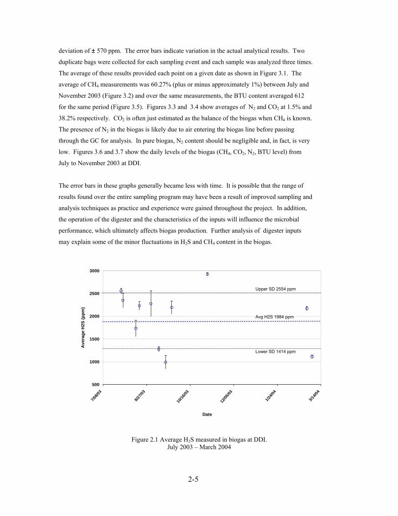
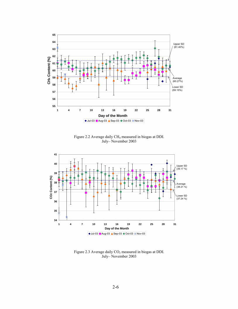
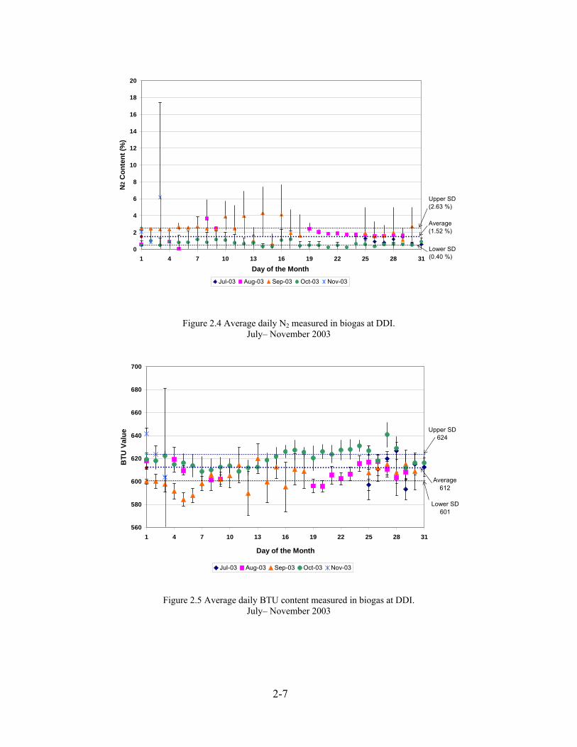
deviation of ± 570 ppm. The error bars indicate variation in the actual analytical results. Two

duplicate bags were collected for each sampling event and each sample was analyzed three times.

The average of these results provided each point on a given date as shown in Figure 3.1. The

average of CH4 measurements was 60.27% (plus or minus approximately 1%) between July and

November 2003 (Figure 3.2) and over the same measurements, the BTU content averaged 612

for the same period (Figure 3.5). Figures 3.3 and 3.4 show averages of N2 and CO2 at 1.5% and

38.2% respectively. CO2 is often just estimated as the balance of the biogas when CH4 is known.

The presence of N2 in the biogas is likely due to air entering the biogas line before passing

through the GC for analysis. In pure biogas, N2 content should be negligible and, in fact, is very

low. Figures 3.6 and 3.7 show the daily levels of the biogas (CH4, CO2, N2, BTU level) from

July to November 2003 at DDI.

The error bars in these graphs generally became less with time. It is possible that the range of

results found over the entire sampling program may have been a result of improved sampling and

analysis techniques as practice and experience were gained throughout the project. In addition,

the operation of the digester and the characteristics of the inputs will influence the microbial

performance, which ultimately affects biogas production. Further analysis of digester inputs

may explain some of the minor fluctuations in H2S and CH4 content in the biogas.

500

1000

1500

2000

2500

3000

7/08/0

3

8/27/0

3

10/16

/03

12/05

/03

1/24/0

4

3/14/0

4

Date

Ave

rage

H2S

(ppm

)

Avg H2S 1984 ppm

Upper SD 2554 ppm

Lower SD 1414 ppm

Figure 2.1 Average H S measured in biogas at DDI. 2

July 2003 – March 2004

2-5

55

56

57

58

59

60

61

62

63

64

65

1 4 7 10 13 16 19 22 25 28 31

Day of the Month

CH

4 Con

tent

(%)

Jul-03 Aug-03 Sep-03 Oct-03 Nov-03

Upper SD (61.40%)

Lower SD (59.15%)

Average(60.27%)

Figure 2.2 Average daily CH measured in biogas at DDI. 4

July– November 2003

34

35

36

37

38

39

40

41

1 4 7 10 13 16 19 22 25 28 31Day of the Month

CO

2 C

onte

nt (%

)

Jul-03 Aug-03 Sep-03 Oct-03 Nov-03

Upper SD(39.17 %)

Average (38.21 %)

Lower SD (37.24 %)

Figure 2.3 Average daily CO measured in biogas at DDI. 2

July– November 2003

2-6

0

2

4

6

8

10

12

14

16

18

20

1 4 7 10 13 16 19 22 25 28 31Day of the Month

N2

Con

tent

(%)

Jul-03 Aug-03 Sep-03 Oct-03 Nov-03

Upper SD(2.63 %)

Average(1.52 %)

Lower SD(0.40 %)

Figure 2.4 Average daily N measured in biogas at DDI. 2July– November 2003

560

580

600

620

640

660

680

700

1 4 7 10 13 16 19 22 25 28 31

Day of the Month

BTU

Val

ue

Jul-03 Aug-03 Sep-03 Oct-03 Nov-03

Upper SD 624

Average 612

Lower SD 601

Figure 2.5 Average daily BTU content measured in biogas at DDI.

July– November 2003

2-7

0

10

20

30

40

50

60

70

7/23/0

3

8/13/0

3

9/03/0

3

9/24/0

3

10/15

/03

11/05

/03

Date

Com

pone

nt (%

)

CH4 N2 CO2

Figure 2.6 Raw biogas analysis at DDI.

July– November 2003

560

570

580

590

600

610

620

630

640

650

660

670

7/25/0

3

8/15/0

39/5

/03

9/26/0

3

10/17

/03

11/7/

03

Date

BTU

Figure 2.7 Raw biogas BTU at DDI.

July– November 2003

2-8

0

1000

2000

3000

4000

5000

6000

7000

8000

9000

9-May

-03

28-Ju

n-03

17-A

ug-03

6-Oct-

03

25-N

ov-03

14-Ja

n-04

4-Mar

-04

23-A

pr-04

Date

Avg

H2S

(ppm

)

AA Dairy DDI Matlink Noblehurst Twin Birch

Figure 2.8 Average H S concentrations at 5 dairy farms in upstate New York. 2

July 2003 – March 2004

Figure 3.8 illustrates the variation over time and between the five farms for the concentration of H2S in the

biogas. This clearly indicates that specific characteristics of digester systems such as environmental

conditions, animal feed, water, addition of other organic materials to the digester may influence the

concentration of H2S in the biogas generated. Of particular note is that the H2S concentrations at Matlink is

substantially less than the other farms and is potentially attributable to co-digestion with food wastes and

manure. Little formal work in this area has been completed, however, “a few dairy farms with anaerobic

digesters in the U.S. have tried mixing food wastes with dairy manure for biogas production. Successful

results have been reported with increased biogas production and better gas quality” (Scott and Ma, 2004).

Preliminary analysis indicates ambient temperature may affect measured CH4 content in the biogas. By

graphing methane production against ambient temperatures from July 25 to November 3, 2003, a trend was

identified as shown in Figure 3.9

for the period of August 22 – August 28, 2003.

For those values greater than the standard deviation 61.4% (less than 6% of all data points), the average

ambient temperature for all of these points was 51.7 F. The average temperature for the values of CH4

production less than the lower standard deviation (59.15%) was 61.0 F. Further statistical analsyis is given

Table 3.1.

2-9

55

56

57

58

59

60

61

62

63

22/08/03

23/08/03

24/08/03

25/08/03

26/08/03

27/08/03

28/08/03

Date

% C

H4

35

40

45

50

55

60

65

70

75

80

85

90

Tem

pera

ture

(F)

% CH4 Temperature (F)

Figure 2.9 Methane generation with ambient temperature at DDI. August 22 – 28, 2003

Table 2.1 Analysis of various ambient temperature ranges at DDI.

July – November, 2003

Temp Range T ≥ 70 F 70 > T ≥ 50 F 50 > T ≥ 30 F

No. Data points in range 61 145 162

% of total data points (2441) 2.5% 6% 6.6%

Thus, it appears that ambient temperatures may have a small effect on CH4 content of biogas at

DDI. However, the explanantion for the variation of CH4 content with temperature, whether due to

GC sensitivity to ambient temperature changes or a function in biogas volumetric change as a

function of temperature variations is not resolved. Additional graphs depicting the variation in

CH4 content on a daily, weekly and monthly basis are provided in the Appendix B. Temperatures

shown in these figures are ambient temperatures and not the biogas temperature itself.

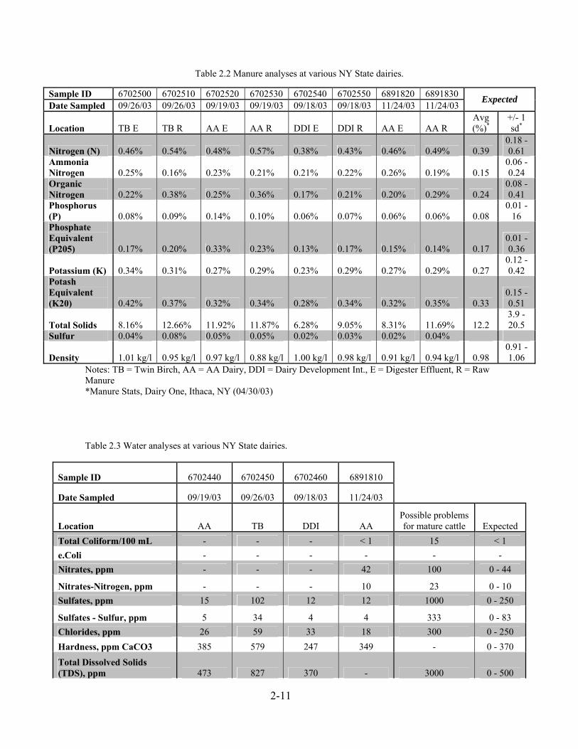
MANURE, WATER, AND FORAGE ANALYSES Analyses of manure and water for four farms are given in Tables 3.2 and 3.3. Of special interest is

the fact that Twin Birch has a much higher concentration of sulfur in the water compared to the

other three farms. This may suggest that the significantly higher H2S concentration (>6000 ppm)

in the biogas at Twin Birch is at least partially attributed to the sulfur in the water.

2-10

2-11

Table 2.2 Manure analyses at various NY State dairies.

Notes: TB = Twin Birch, AA = AA Dairy, DDI = Dairy Development Int., E = Digester Effluent, R = Raw Manure *Manure Stats, Dairy One, Ithaca, NY (04/30/03)

Table 2.3 Water analyses at various NY State dairies.

Sample ID 6702440 6702450 6702460 6891810

Date Sampled 09/19/03 09/26/03 09/18/03 11/24/03

Location AA TB DDI AA Possible problems for mature cattle Expected

Total Coliform/100 mL - - - < 1 15 < 1 e.Coli - - - - - - Nitrates, ppm - - - 42 100 0 - 44

Nitrates-Nitrogen, ppm - - - 10 23 0 - 10 Sulfates, ppm 15 102 12 12 1000 0 - 250

Sulfates - Sulfur, ppm 5 34 4 4 333 0 - 83 Chlorides, ppm 26 59 33 18 300 0 - 250 Hardness, ppm CaCO3 385 579 247 349 - 0 - 370

Total Dissolved Solids (TDS), ppm 473 827 370 - 3000 0 - 500

Sample ID 6702500 6702510 6702520 6702530 6702540 6702550 6891820 6891830 Date Sampled 09/26/03 09/26/03 09/19/03 09/19/03 09/18/03 09/18/03 11/24/03 11/24/03

Expected

Location TB E TB R AA E AA R DDI E DDI R AA E AA R Avg (%)*

+/- 1 sd*

Nitrogen (N) 0.46% 0.54% 0.48% 0.57% 0.38% 0.43% 0.46% 0.49% 0.39 0.18 - 0.61

Ammonia Nitrogen 0.25% 0.16% 0.23% 0.21% 0.21% 0.22% 0.26% 0.19% 0.15

0.06 - 0.24

Organic Nitrogen 0.22% 0.38% 0.25% 0.36% 0.17% 0.21% 0.20% 0.29% 0.24

0.08 - 0.41

Phosphorus (P) 0.08% 0.09% 0.14% 0.10% 0.06% 0.07% 0.06% 0.06% 0.08

0.01 - 16

Phosphate Equivalent (P205) 0.17% 0.20% 0.33% 0.23% 0.13% 0.17% 0.15% 0.14% 0.17

0.01 - 0.36

Potassium (K) 0.34% 0.31% 0.27% 0.29% 0.23% 0.29% 0.27% 0.29% 0.27 0.12 - 0.42

Potash Equivalent (K20) 0.42% 0.37% 0.32% 0.34% 0.28% 0.34% 0.32% 0.35% 0.33

0.15 - 0.51

Total Solids 8.16% 12.66% 11.92% 11.87% 6.28% 9.05% 8.31% 11.69% 12.2 3.9 - 20.5

Sulfur 0.04% 0.08% 0.05% 0.05% 0.02% 0.03% 0.02% 0.04%

Density 1.01 kg/l 0.95 kg/l 0.97 kg/l 0.88 kg/l 1.00 kg/l 0.98 kg/l 0.91 kg/l 0.94 kg/l 0.98 0.91 - 1.06

2-12

Calcium (Ca), ppm 119.6 168 76.3 107.6 500 0 - 100 Magnesium (Mg), ppm 21 38.8 13.7 19.6 125 0 - 29 Potassium (K), ppm - - - < 0.1 20 0 - 20 Sodium (Na), ppm 16.9 26 23.5 13.5 300 0 - 100 Iron (Fe), ppm <0.01 <0.01 <0.01 - 0.3 (taste) 0 - 0.3 pH 7.6 7.6 7.9 7.8 <5.5 or >8.5 6.8 - 7.5

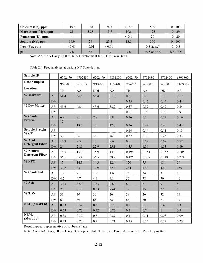
Note: AA = AA Dairy, DDI = Dairy Development Int., TB = Twin Birch Table 2.4 Feed analyses at various NY State dairies.

Sample ID 6702470 6702480 6702490 6891800 6702470 6702480 6702490 6891800 Date Sampled

9/26/03 9/19/03 9/18/03 11/24/03 9/26/03 9/19/03 9/18/03 11/24/03 Location

TB AA DDI AA TB AA DDI AA AF 54.4 56.6 56.4 61.8 0.21 0.2 0.19 0.17 % Moisture

DM 0.45 0.46 0.44 0.44 AF 45.6 43.4 43.6 38.2 0.37 0.39 0.42 0.34 % Dry Matter

DM 0.81 0.9 0.96 0.9 AF 6.9 8.1 7.8 6.8 0.16 0.2 0.17 0.16 % Crude

Protein DM

15. 18.7 18 17.7 0.36 0.47 0.4 0.43

AF 0.14 0.14 0.11 0.13 Soluble Protein % CP

DM 39 36 38 46 0.32 0.32 0.25 0.33 AF 10.9 9.5 10 9.6 0.61 0.59 0.67 0.72 % Acid

Detergent Fiber DM 24 21.9 22.9 25.1 1.35 1.36 1.53 1.89 AF 16.5 15.3 15.9 14.6 0.194 0.154 0.152 0.105 % Neutral

Detergent Fiber DM 36.1 35.4 36.5 38.2 0.426 0.355 0.348 0.274 AF 17 14.3 14.3 12.4 120 75 184 59 % NFC

DM 37.2 33 32.9 32.6 264 172 422 155 AF 1.9 2.1 1.9 1.6 26 34 31 15 % Crude Fat

DM 4.2 4.7 4.4 4.1 56 78 70 40 AF 3.33 3.53 3.63 2.84 8 6 9 4 % Ash

DM 7.3 8.13 8.33 7.44 17 15 22 10 AF 31 30 30 26 39 26 32 14 % TDN

DM 69 69 68 68 86 60 73 37 AF 0.33 0.32 0.31 0.28 0.2 0.3 0.4 0.3 NEL, (Mcal/Lb)

DM 0.73 0.73 0.72 0.72 0.4 0.7 1 0.9 AF 0.33 0.32 0.31 0.27 0.11 0.11 0.08 0.09 NEM,

(Mcal/Lb) DM 0.73 0.73 0.71 0.71 0.25 0.25 0.17 0.25

Results appear representative of soybean silage Note: AA = AA Dairy, DDI = Dairy Development Int., TB = Twin Birch, AF = As fed, DM = Dry matter

BIOGAS PROCESSING

A significant goal of this project has been to consider the potential for biofiltration to reduce

(remove) the concentration of H2S because all energy converters need to operate at H2S levels

significantly less than that found in raw biogas. Zicari (2003) has considered the utilization of cow-

manure compost for removal of H2S from AD biogas using small-scale reactors. Slipstreams of AD

biogas (approximately 60% methane, 40 % carbon dioxide and 1000- 4000 ppm of H2S) from an

operating system at AA Dairy and Dairy Development International (DDI) were passed through

reactor sections of a cow manure compost mixture within polyvinyl chloride cylinders of 0.1 m in

diameter and 0.5 m in length. The mature cow-manure compost (60 days in AA Dairy’s outdoor

windrow system) was mixed in a 1:1 ratio with dry maple wood chips. Columns have shown over

90% removal efficiency for the early stages of these tests (Figure 4.1 and 4.2). The removal

efficiency (RE) is defined as the difference in inlet and outlet concentrations of H2S divided by the

inlet concentration. Column A (Figure 4.1) continued to operate with RE’s above 85% for 33 days

before falling off to 55% by day 44. Column B (Figure 4.2 ) decreased to 50 – 60% RE after 16

days and performed at this level for the rest of the run, except for an increase to around 80% RE between days 37-40. Runs were terminated after 44 days, as both columns A and B neared 50%

RE, to examine the compost for sulfur accumulation. The H2S elimination capacity of columns A

and B ranged from 24 – 112 and 16 – 118 g H2S/m3 /hr, respectively. The total mass of Hpacking 2S

removed from the gas during these experiments is estimated at 135 and 127 g H2S, respectively for

columns A and B. These values approach a maximum value of 130 g H2S/m3packing/hr reported for

organic media by Yang and Allen (1994).

0%

10%

20%

30%

40%

50%

60%

70%

80%

90%

100%

0.0 5.0 10.0 15.0 20.0 25.0 30.0 35.0 40.0 45.0

Run Time (Days)

Rem

oval

Effi

cien

cy (%

)

0

500

1000

1500

2000

2500

3000

3500

4000

4500

5000

Inle

t H2S

Con

cent

ratio

n (p

pm)

Figure 3.1 Removal efficiencies (○) and inlet concentrations (■) for Column A.

3-1

Ambient and bed temperatures were measured for a portion of the study but not throughout. A

proposed explanation for the decrease in removal efficiency for Figure 4.2 around day 10 is that an

upper critical temperature limit was surpassed, causing the number of active bacterial populations

to decrease. Elevated bed temperatures, over both inlet gas and ambient temperatures, indicate that

exothermic biological, chemical, or physical reactions are occurring in the bed and could

potentially be used to track bed activity or viability. During the first 9 days, both columns

exhibited an increased bed temperature of about 5° C over the inlet gas temperature. At day 10,

corresponding with the upset in removal efficiency noticed for column B (Figure 4.3), the margin

of bed temperature rise over inlet gas temperature fell to around 2° C. Column A, which

maintained higher removal efficiency during the first 17 days, also displayed a higher bed

temperature elevation of around 4° C during days 10-18.

Columns C and D (Figures 4.3 and 4.4) were operated for 83 days between June and September

2003. In columns C and D, removal efficiencies were between 80-100% for the first 20 days. Sharp

decreases in removal efficiencies, to 61% and 54% for columns C and D, respectively, were

observed between days 20 and 21. For days 21-83, columns C and D behaved similarly with

removal efficiencies varying between 29% and 93%. Relative maxims in removal efficiencies were

observed for trial C on days 31 and 59, at 86% and 93%, with relative minima of 39%, 29%, and

34%, occurring on days 26, 37, and 67 respectively (Figure 4.3). Relative maxims in removal

efficiencies for trial D were also observed on days 31 and 59, at 84% and 83%, with relative

minima of 35%, 34%, and 31%, also occurring on days 26, 37, and 67, respectively (Figure 4.4).

3-2

0%

10%

20%

30%

40%

50%

60%

70%

80%

90%

100%

0.0 5.0 10.0 15.0 20.0 25.0 30.0 35.0 40.0 45.0

Run Time (Days)

Rem

oval

Effi

cien

cy (%

)

0

500

1000

1500

2000

2500

3000

3500

4000

4500

5000

Inle

t H2S

Con

cent

ratio

n (p

pm)

Figure 3.2 Removal efficiency (○) and inlet concentration (■) for Column B.

0%

10%

20%

30%

40%

50%

60%

70%

80%

90%

100%

0 10 20 30 40 50 60 70 80

Run Time (Days)

Rem

oval

Effi

cien

cy (%

)

15

25

35

45

55

65

75

85

95

Max

imum

Dai

ly B

ed T

empe

ratu

re (

o C)

Figure 3.3 Removal efficiency (○) and maximum daily temperatures (▲) for Column C.

Instrument failures were responsible for data loss between days 67-83, and average inlet

concentrations with removal efficiencies of 50% were assumed for the following calculations.

Elimination capacities ranged from 19-46 (average 32) g H2S/m3packing/hr for column C, and 17-46

(average 27) g H2S/m3 /hr for column D. packing

3-3

0%

10%

20%

30%

40%

50%

60%

70%

80%

90%

100%

0 10 20 30 40 50 60 70 80

Run Time (Days)

Rem

oval

Effi

cien

cy (%

)

15

25

35

45

55

65

75

85

95

Max

imum

Dai

ly B

ed T

empe

ratu

re (

o C)

Figure 3.4 Removal efficiency (○) and maximum daily bed temperatures (▲) for Column D.

The highest recorded maximum daily media temperatures for columns C and D (Figures 4.3 and 4.4),

35.9° C and 34.8° C, respectively, occured on day 18, two days prior to the decline in effectiveness

around day 20. Additionally, relative maxims in the maximum daily bed temperatures occured on

days 32 and 57, corresponding closely with maxims in column removal efficiencies followed shortly

by reductions in performance. These data, and that for trials A and B, are suggestive of the existence

of a very tight optimum temperature operating range, which, when exceeded, creates biological upset

and a subsequent reduction in performance. Maximum daily bed temperatures followed maximum

daily ambient temperatures (± 3° C), and relative maxims or minima in the bed temperatures

corresponded to those in the ambient temperature record.

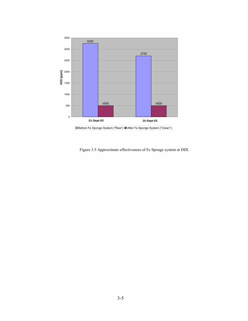
“IRON SPONGE” RESULTS

DDI did install an iron sponge system to “clean” H2S from raw biogas. No systematic and consistent

measurements were obtained from this system. Two measurements were taken about a week apart

with Draeger indicator tubes to obtain a rough assessment of the effect of the iron sponge.

Unfortunately, follow up measumenets over time are not available to assess the life and effectiveness

of the iron sponge. The two measuremnets illustrated in Figure 4.5 do show a removal effect early

after the istallation of the system at DDI.

3-4

0

500

1000

1500

2000

2500

3000

3500

H2S

(ppm

)

Before Fe Sponge System ("Raw") After Fe Sponge System ("Clean")

01-Sept-03 10-Sept-03

3250

2700

≤500 ≤500

Figure 3.5 Approximate effectiveness of Fe Sponge system at DDI.

3-5

ECONOMONIC ASSESSMENT OF DAIRY-DERIVED BIOGAS INJECTION INTO THE NATURAL GAS PIPELINE

Background

Biogas recovery and processing (including cleaning and upgrading) for injection into the natural gas

pipeline depends primarily on the financial viability of such a project. From the point of view of the farmer,

the use of anaerobic digestion (AD) technology is often driven by community demands for odor control and

concentrated animal feeding operations (CAFO) regulations. Because farmers increasingly control odor and

manage manure by using AD, it makes sense from an environmental and economical perspective to explore

biogas utilization options. However, processing biogas to natural gas pipeline quality, has received limited

consideration because it is generally perceived to be too expensive. Nevertheless, we believe the idea is

worthy of serious analysis, given the limitations and drawbacks to standard cogeneration technologies.

The main limitations to upgrading biogas to natural gas quality are not technical but economical and

political. The willingness of a buyer to purchase the upgraded biogas is crucial and a buyer must be

established during the initial stages of the project. A minimum price that the buyer will pay for the biogas

during the lifetime of the project also must be established. In addition, it is essential to establish who will

purchase the processed biogas gas in order to design the system to meet the gas quality needs of the buyer.

One buyer, for instance, may accept processed biogas into the natural gas pipeline that has at least 95%

CH4, while another buyer may only accept gas with at least 98% CH4. In addition to gas quality, the amount

of gas the buyer is willing to purchase for injection into the pipeline is vital information. The buyer may

want to be guaranteed that a certain amount of biogas (volume/time) will be available to inject into the line.

The cost of upgrading biogas varies considerably and very few 'hard numbers' are found in the literature.

From the literature review, the limited data that is available pertains mainly to upgrading landfill gas.

Because of this limitation, most of the economic data presented in this chapter is based on data from

sources that have upgraded landfill biogas to natural gas quality. In general, landfill gas (LFG) is

approximately 50-58 % CH4, the primary component of natural gas. The other 42-50 % of the gas is

predominantly CO2, with small amounts of N2 and O2, and trace levels of non-methane organic compounds.

These include alkanes, chlorocarbons, oxygenated compounds, other hydrocarbons, sulfur dioxide and H2S.

Usually, agricultural biogas has more CH4 than LFG (58-65%) and does not contain alkanes, chlorocarbons

and oxygenated compounds.

4-1

4-2

To date, most landfill gas recovery projects utilize the gas in direct applications, such as in boilers or to

heat greenhouses (Goldstein, 2005). Using the landfill gas to generate electricity with diesel engines or

microturbines is another emerging technology. Using LFG as a source of alternate fuel, by upgrading the

gas to a high Btu value for pipeline injection or for vehicle fuel, is less prevalent, although there are several

operational high Btu projects in the United States. As an example of a high Btu application, the LFG from

one relatively small landfill in Monroeville, PA is processed and blended into the natural gas pipeline.

Another project, as an example of a medium-Btu application, is blending non-upgraded LFG (impurities

such as alkanes, chlorocarbons, oxygenated compounds, water, sulfur dioxide and H2S are removed, but not

CO2) into the natural gas pipeline. To keep the amount of CO2 in the pipeline at an acceptable level, the

LFG is blended with natural gas in the pipeline (Landfill Methane Outreach Program, 2004). Table 4.1

below displays some operational projects that convert LFG to natural gas for pipeline injection.

Financial Viability of Upgrading Biogas to Pipeline Because LFG is similar to the biogas produced as a result of AD of manure on a dairy farm, much of the

economic information from LFG processing projects can be applied to dairy biogas processing projects. For

a landfill with 1 million metric tons of waste in place, it is estimated that, on average, 200 million ft3/year

or 550,000 ft3/day of gas will be produced (U.S. EPA Landfill Methane Outreach Program, 1996).

Presently, due to the high cost of cleaning and upgrading LFG, only large landfills that produce substantial

quantities of gas are candidates for converting low Btu LFG to high Btu, pipeline quality gas. From Table

4.1, the smallest landfill from which LFG is upgraded to high Btu gas has two million metric tons of waste

in place.

To compare gas produced in a landfill to the gas produced by AD on a dairy farm, the landfill gas

production can be converted to a ‘cow equivalent’. To determine the amount of biogas a landfill produces

each year, taking into account the decrease in gas production as the waste in the landfill disintegrates, the

EPA LandGem Model was used. The landfill gas generation rate in this model is based on a first order

decomposition model, which estimates the landfill gas generation rate using two parameters:

• Lo, the potential CH4 generation capacity of the waste and

• k, the CH4 generation decay rate, which accounts for how quickly the methane

generation rate decreases, once it reaches its peak rate. The methane generation rate is assumed to be at its peak upon placement of the waste in the landfill. This

model allows the user to enter Lo and k values using test data and landfill specific parameters, or use default

Lo and k values derived from test data collected during the course of research for federal regulations

governing air emissions from municipal solid waste landfills. In this case, k and Lo values

1.550

1.122

4.900

3.600

No Data

No Data

No Data

No Data

4-3

Table 4.1 Operational Medium and High Btu LFG Projects Landfill Methane Outreach Program, December 2004

Landfill Name

Landfill City State

Waste In Place (tons)

Year Landfill Opened

Landfill Closure

Year

Landfill Owner

Organization Project

Start Date

Project Developer

Organization

LFGE Project Type

LFG Flow to Project

(106 scfd)

Johnson County LF Shawnee KS 20,000,000 1979 2030

Deffenbaugh Industries,

Inc. 9/1/2001 South Texas

Treaters High Btu

American LF Waynesburg OH 14,157,332 1975

Waste Management,

Inc. 6/30/2003 Toro Energy,

Inc. Medium

Btu

Pinnacle Road LF Dayton OH 6,150,000 1979 1993

Waste Management,

Inc. 4/1/2003 DTE Biomass

Energy High Btu

Rumpke SLF, Inc. Cincinnati OH 11,500,000 1965 2021

Rumpke Waste, Inc. 1/1/1986

Montauk Energy

Capital/GSF Energy

High Btu 9.000

Stony Hollow LF Dayton OH 7,500,000 1996 2009

Waste Management,

Inc. 4/1/2003 DTE Biomass

Energy High Btu

Monroeville LF Monroeville PA 2,000,000 1971 2035

Waste Management,

Inc. 10/29/2004

Beacon Generating

LLC/Magellan EnviroGas

Partners, LLC High Btu

Valley LF Irwin PA 6,000,000 1990 2025

Waste Management,

Inc. 2/27/2004

Beacon Generating

LLC/Magellan EnviroGas

Partners, LLC High Btu

High Btu

McCarty Road LF Houston TX 28,918,718 1977 2001

Allied Waste Services 1/1/1986

Montauk Energy Capital

High Btu

Pacific Natural Energy, LLC 1/1/2000 City of Dallas 2053 1980 26,470,000 TX Dallas

McCommas Bluff LF

based on USEPA AP-42, Appendix A, Thermal Equivalents of Various Fuels, were used. If a dairy

cow produces approximately 100 ft3/day of biogas, then, averaged over a 10 year period, a landfill with

1 million tons of waste in place will produce approximately as much biogas as 4,800 cows. Landfills

with 2 and 3 million tons of waste in place will produce approximately as much biogas as 9,600 and

14,400 cows, respectively. See Table 8.2, below.

In this case, k and Lo values based on USEPA AP-42, Appendix A, Thermal Equivalents of Various

Fuels, were used. If a dairy cow produces approximately 100 ft3/day of biogas, then, averaged over a

10 year period, a landfill with 1 million tons of waste in place will produce approximately as much

biogas as 4,800 cows. Landfills with 2 and 3 million tons of waste in place will produce approximately

as much biogas as approximately 9,600 and 14,400 cows, respectively (Table 4.2).

Table 4.2 Landfill Gas Production and Dairy Biogas Equivalent Gas Production With 1 Million

Tons of Waste in Place (ft

Gas Production With 2 Million

Tons of Waste in Place (ft

Gas Production With 3 Million

Tons of Waste in Place (ft3 3 3YEAR /yr) /yr) /yr)

1 200,000,000 400,000,000 600,000,000 2 194,000,000 388,000,000 582,000,000 3 188,180,000 376,360,000 564,540,000 4 182,534,600 365,069,200 547,603,800 5 177,058,562 354,117,124 531,175,686 6 171,746,805 343,493,610 515,240,415 7 166,594,401 333,188,802 499,783,203 8 161,596,569 323,193,138 484,789,707 9 156,748,672 313,497,344 470,246,016 10 152,046,212 304,092,423 456,138,635

Total Biogas Production over 10 Years (ft3) 1,750,505,821 3,501,011,641 5,251,517,462

Average Biogas Production over 10 Years (ft3) 175,050,582 350,101,164 525,151,746

Equivalent Number of Cows 4,796 9,592 14,388

4-4

Effect of Farm Size

We will assess the effect of farm size on the financial viability of injection to the natural gas pipeline in

this section. We assume that the biogas from dairies has the parameter values of CH4 = 60%, CO2 =

38%, N2 and O2 Combined = 2%, H2S = 3,000 ppm.

Recent studies show that adding food waste to the digester increases the biogas generation potential

substantially. For further information, see A Guideline for Co-Digestion of Food Wastes in Farm-Based

Anaerobic Digesters (Scott and Ma, December, 2004) and Potential of Using Food Wastes In Farm-

Based Anaerobic Digesters (Scott and Ma, January, 2004), which are available at

http://www.manuremanagement.cornell.edu. For future projects that consider upgrading dairy biogas to

natural gas pipeline quality, the addition of food waste should be considered to increase the biogas

generation potential.

This analysis assumes that the minimum gas quality standards for injection into the natural gas pipeline

are CH4 = 97%, CO2 = 2%, N2 and O2 Combined = 1%, H2S < 4ppm. Given these assumptions, the gas

processing system must consist of an H2S removal system, a gas conditioning system, a CO2, N2 and O2

removal system, and a compressor to increase the treated gas pressure to meet pipeline distribution

pressure. A description of the main components of the system is described in Figure 4.1 for a

conceptual design of the system. Vessels V1 and V2 are used for H2S removal. Vessels V3, V4 and V5

are pressure swing adsorption vessels (PSA).

H2S Removal System This system consists of two vessels containing iron oxide media, such as iron sponge (red iron oxide

impregnated on wood chips), in parallel. The vessels are used in parallel so that if one vessel is being

cleaned or the media is being changed, the other will operate, allowing the H2S system to run

continuously.

Gas Conditioning Package The system consists of a coalescing filter, a gas/gas exchanger, a chiller and a gas/liquid exchanger to

remove water and impurities from the biogas. The coalescing filter is used for the separation of liquid

aerosols and droplets from a gas. It is recommended that as much water and impurities as possible be

removed before the biogas enters the PSA. Much of the water will be removed before entering the H2S

removal system via condensation as the biogas moves through the pipe connecting the digester and

the H2S removal system. This will reduce the amount of water that the gas-conditioning package has

to remove.

4-5

4-6

Gas Upgrading System To remove constituents of the biogas that decrease its calorific value and Wobbe Index, a PSA system

may be used. The Wobbe Index is defined as: the Calorific Value of Fuel/(Specific Gravity of the

Fuel)1/2 The Wobbe Index for CH4 is approximately 1220 Btu/cubic foot. The PSA system shown in the

Figure 4.1 consists of 3 vessels in series, which separates out CO2, N2 and O2 from the methane rich gas

by the adsorption/desorption of CO2, N2 and O2 onto activated carbon or zeolites at different pressures.

Two Stage Compression This step is necessary to increase the pressure of the treated biogas to meet the pipeline pressure

specification. Natural gas that is transported through larger pipelines over long distances is at high

pressures ranging from 200 to 1500 pounds per square inch (psi). This pressure reduces the volume of

the natural gas being transported (by up to 600 times), and provides a propellant force to move the

natural gas through the pipeline (NaturalGas.Org, 2004). In shorter, localized or district natural gas

pipelines may be pressurized to 100 psi or less.

Capital Cost of Biogas Processing Equipment Table 4.3 shows capital cost data for a biogas processing system that will clean and upgrade dairy

biogas to natural gas quality. The cost data were adapted from that provided by Applied Filter

Technology (AFT). AFT is a research and engineering company that has designed, constructed and

built LFG processing systems that remove CO2 and contaminants from the gas stream. The economic

data provided by AFT was checked again costing information provided by another company

(Cogeneration Technologies, a subsidiary of EcoGeneration™ Solutions, LLC) and was found to be

comparable. According to AFT, the capital cost to install a biogas processing plant for a 500 cow dairy

and 1,000 cow dairy despite the difference in biogas volume is approximately the same due to economy

of scale.

Operation and Maintenance (O&M) Costs for Biogas Processing Equipment Table 4.4 displays the yearly O&M costs to keep the biogas processing system functional and in good

working condition. The data were adapted from that provided by AFT. The O&M costs presented

below are based on AFT’s experience in operating several LFG processing systems over the past

decade. As with capital costs, AFT estimates that the operational and maintenance costs for a 500 and

1,000 cow biogas processing plant are approximately the same.

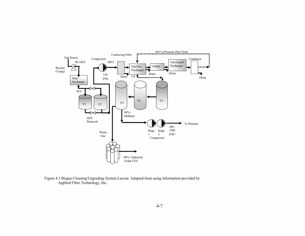
Waste Gas

Booster (5 psig)

Drain

40 F at Pressure Dew Point

To Pipeline

Gas Source

Gas/Gas Exchanger

Coalescing Filter Compressor

V3

H2S Removal

V1 V2

Drain 77F

V4 V5

200 -1500 psig +

Stage 1

98%+ Methane

130 psig

Stage 2

Heat Exchanger

90-100 F

80 F

98%+ Industrial Grade CO2

200 F Gas/Liquid Exchanger Chiller

Condenser

Compressor

Drain Drain

4-7

Figure 4.1 Biogas Cleaning/Upgrading System Layout. Adapted from using information provided by

Applied Filter Technology, Inc.

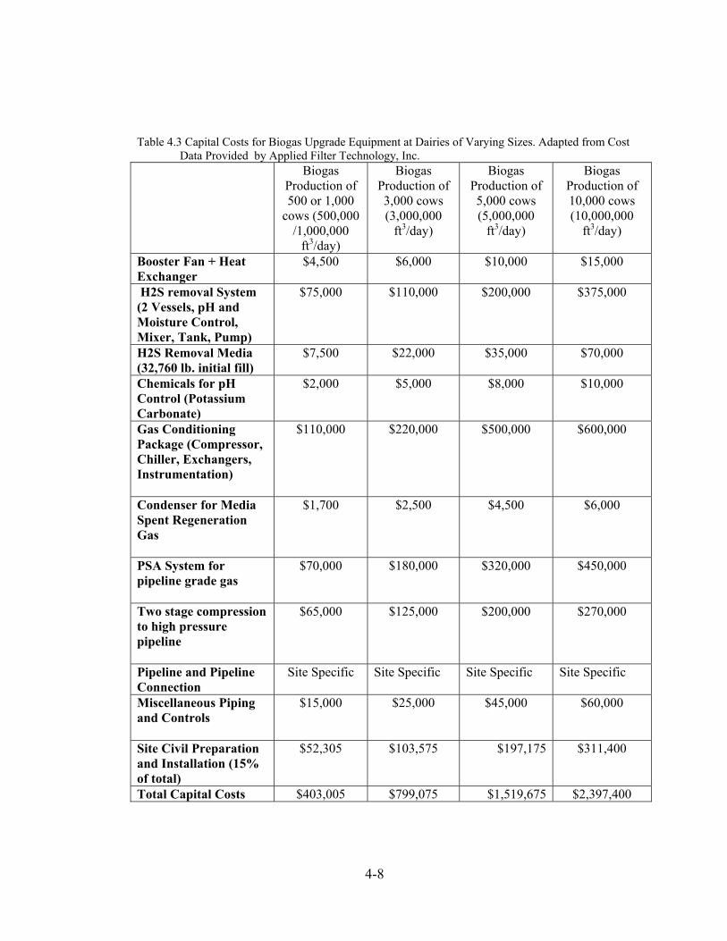
Table 4.3 Capital Costs for Biogas Upgrade Equipment at Dairies of Varying Sizes. Adapted from Cost

Data Provided by Applied Filter Technology, Inc. Biogas

Production of 3,000 cows (3,000,000

ft

Biogas Production of 500 or 1,000

cows (500,000 /1,000,000

Biogas Production of 5,000 cows (5,000,000

ft

Biogas Production of 10,000 cows (10,000,000

ft

3 3 3/day) /day) /day) 3ft /day)

Booster Fan + Heat Exchanger

$6,000 $4,500 $10,000 $15,000

H2S removal System (2 Vessels, pH and Moisture Control, Mixer, Tank, Pump)

$110,000 $75,000 $200,000 $375,000

H2S Removal Media (32,760 lb. initial fill)

$22,000 $7,500 $35,000 $70,000

Chemicals for pH Control (Potassium Carbonate)

$5,000 $2,000 $8,000 $10,000

Gas Conditioning Package (Compressor, Chiller, Exchangers, Instrumentation)

$220,000 $110,000 $500,000 $600,000

Condenser for Media Spent Regeneration Gas

$2,500 $1,700 $4,500 $6,000

PSA System for pipeline grade gas

$180,000 $70,000 $320,000 $450,000

Two stage compression to high pressure pipeline

$125,000 $200,000 $270,000 $65,000

Pipeline and Pipeline Connection

Site Specific Site Specific Site Specific Site Specific

Miscellaneous Piping and Controls

$25,000 $15,000 $45,000 $60,000

Site Civil Preparation and Installation (15% of total)

$52,305 $103,575 $197,175 $311,400

Total Capital Costs $403,005 $799,075 $1,519,675 $2,397,400

4-8

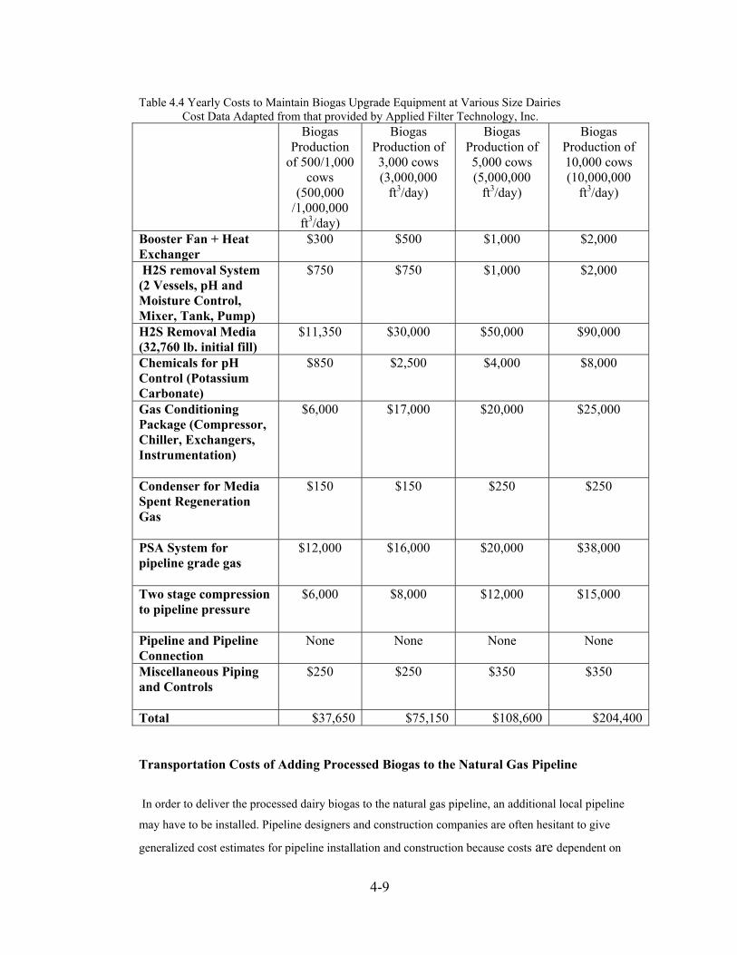
Table 4.4 Yearly Costs to Maintain Biogas Upgrade Equipment at Various Size Dairies Cost Data Adapted from that provided by Applied Filter Technology, Inc.

Biogas Production

of 500/1,000 cows

(500,000 /1,000,000

Biogas Production of 3,000 cows (3,000,000

ft

Biogas Production of 5,000 cows (5,000,000

ft

Biogas Production of 10,000 cows (10,000,000

ft

3 3 3/day) /day) /day)

3ft /day) Booster Fan + Heat Exchanger

$500 $300 $1,000 $2,000

H2S removal System (2 Vessels, pH and Moisture Control, Mixer, Tank, Pump)

$750 $750 $1,000 $2,000

H2S Removal Media (32,760 lb. initial fill)

$30,000 $11,350 $50,000 $90,000

Chemicals for pH Control (Potassium Carbonate)

$2,500 $850 $4,000 $8,000

Gas Conditioning Package (Compressor, Chiller, Exchangers, Instrumentation)

$17,000 $6,000 $20,000 $25,000

Condenser for Media Spent Regeneration Gas

$150 $150 $250 $250

PSA System for pipeline grade gas

$16,000 $20,000 $38,000 $12,000

Two stage compression to pipeline pressure

$8,000 $6,000 $12,000 $15,000

Pipeline and Pipeline Connection

None None None None

Miscellaneous Piping and Controls

$250 $250 $350 $350

Total $37,650 $75,150 $108,600 $204,400 Transportation Costs of Adding Processed Biogas to the Natural Gas Pipeline In order to deliver the processed dairy biogas to the natural gas pipeline, an additional local pipeline

may have to be installed. Pipeline designers and construction companies are often hesitant to give

generalized cost estimates for pipeline installation and construction because costs are dependent on

4-9

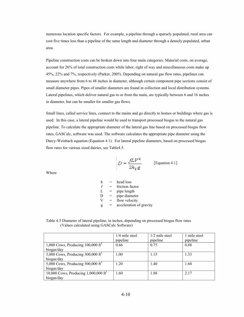
numerous location specific factors. For example, a pipeline through a sparsely populated, rural area can

cost five times less than a pipeline of the same length and diameter through a densely populated, urban

area. Pipeline construction costs can be broken down into four main categories. Material costs, on average,

account for 26% of total construction costs while labor, right of way and miscellaneous costs make up

45%, 22% and 7%, respectively (Parker, 2005). Depending on natural gas flow rates, pipelines can

measure anywhere from 6 to 48 inches in diameter, although certain component pipe sections consist of

small diameter pipes. Pipes of smaller diameters are found in collection and local distribution systems.

Lateral pipelines, which deliver natural gas to or from the main, are typically between 6 and 16 inches

in diameter, but can be smaller for smaller gas flows.

Small lines, called service lines, connect to the mains and go directly to homes or buildings where gas is

used. In this case, a lateral pipeline would be used to transport processed biogas to the natural gas

pipeline. To calculate the appropriate diameter of the lateral gas line based on processed biogas flow

rates, GASCalc, software was used. The software calculates the appropriate pipe diameter using the

Darcy-Weisbach equation (Equation 4.1). For lateral pipeline diameters, based on processed biogas

flow rates for various sized dairies, see Table4.5.

Where

h = head loss f = friction factor L = pipe length D = pipe diameter V = flow velocity g = acceleration of gravity

Table 4.5 Diameter of lateral pipeline, in inches, depending on processed biogas flow rates (Values calculated using GASCalc Software)

1/4 mile steel pipeline

1/2 mile steel pipeline

1 mile steel pipeline

1,000 Cows, Producing 100,000 ft3 biogas/day

0.66 0.75 0.88

3,000 Cows, Producing 300,000 ft3 biogas/day

1.00 1.15 1.33

5,000 Cows, Producing 500,000 ft3 biogas/day

1.20 1.40 1.60

10,000 Cows, Producing 1,000,000 ft3 biogas/day

1.60 1.88 2.17

{Equation 4.1}

4-10

Pipeline Costs Once the appropriate pipe diameter is calculated, it is possible to determine the cost to install the

pipeline of given length. Table 4.6 illustrates the material and labor costs for installing pipelines of

various diameters, per linear foot. The cost data are from R.S. Means, a software package that is an

industry standard for pricing civil, environmental and mechanical engineering projects. In order to

choose the correct diameter of pipe to be installed, the gas flow rate through the pipe must be known.

The gas flow rate is based on the digester’s biogas generation potential and the number of cows on the

dairy farm.

Table 4.6 Pipeline Construction and Installation Costs

(Data from R.S. Means, CostWorks 2005, Equipment and Labor Rates for Syracuse, NY)

Unit Bare Material Bare Labor Bare Total Total, Including Company

Overhead and Profit

(Carbon Steel)

¼” Diameter Linear Foot

6.15 5.10 11.25 14.45

3/8” Diameter Linear Foot

7.35 5.20 12.55 15.95

½” Diameter Linear Foot

9.50 5.35 14.85 18.50

¾” Diameter Linear Foot

11.80 5.40 17.20 21.00

1” Diameter Linear Foot

15.45 6.15 21.60 26.00

1-1/4” Linear Foot

18.90 6.50 25.40 33.00

1-1/2” Linear Foot

25.70 7.20 32.90 42.10

2” Diameter Linear Foot

31.50 8.70 40.20 47.50

In order to assess the economic feasibility of upgrading biogas to natural gas quality for injection into

the natural gas pipeline when the biogas processing station is not located near the pipeline, three

pipeline scenarios were considered. Table 4.7 illustrates the costs of transporting upgraded biogas ¼

mile, ½ mile and 1 mile to the natural gas pipeline. In addition to the cost of the pipe installation itself, it is standard to add 25% to 50% of the cost to include valves and fittings (R.S. Means, 2005).

In order to install the pipeline underground, a trench must be dug. Table 4.8 demonstrates the cost for

digging the trench in which the lateral pipeline is placed. Depending on local regulations, location of

the water table, depth to frost and the location of other utility lines, the trench may be anywhere from 4

to 14 feet deep.

4-11

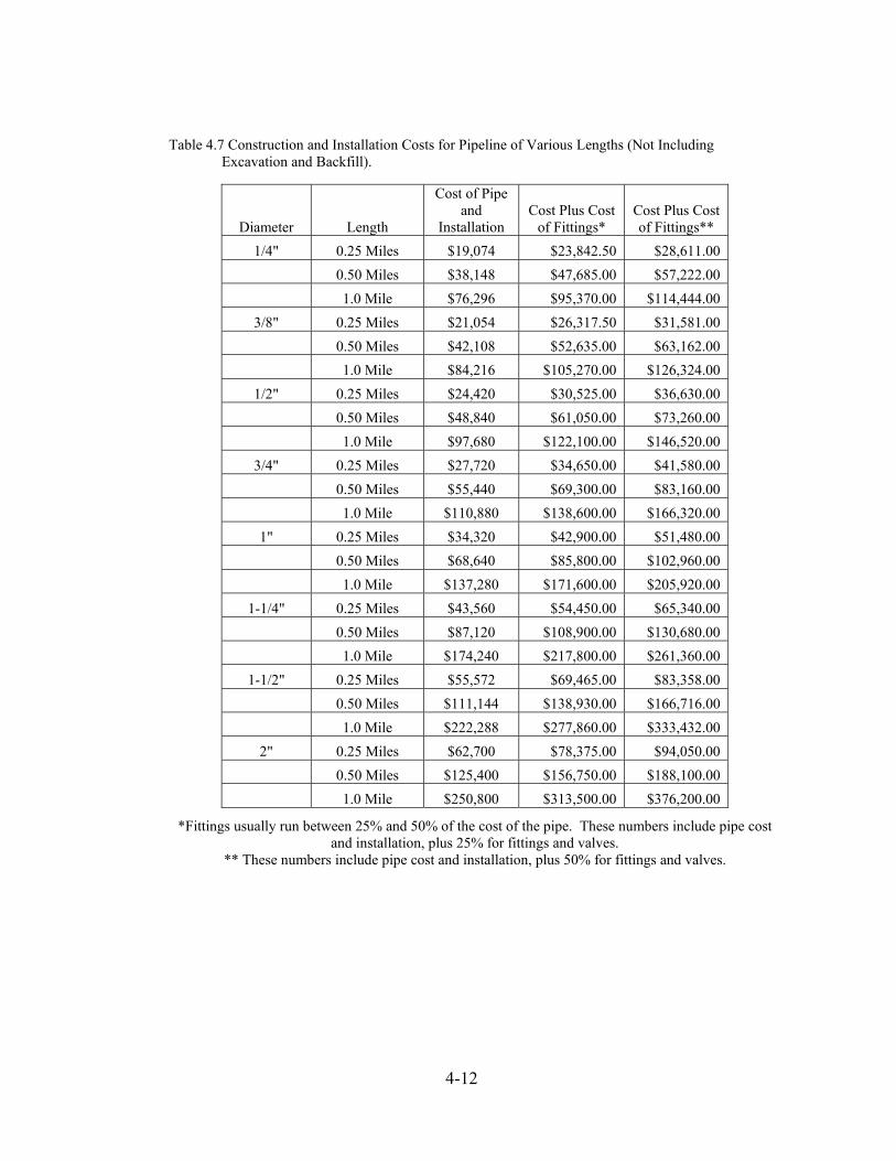
Table 4.7 Construction and Installation Costs for Pipeline of Various Lengths (Not Including

Excavation and Backfill).

*Fittings usually run between 25% and 50% of the cost of the pipe. These numbers include pipe cost and installation, plus 25% for fittings and valves.

** These numbers include pipe cost and installation, plus 50% for fittings and valves.

Diameter Length

Cost of Pipe and

Installation Cost Plus Cost

of Fittings* Cost Plus Cost of Fittings**

1/4" 0.25 Miles $19,074 $23,842.50 $28,611.00 0.50 Miles $38,148 $47,685.00 $57,222.00 1.0 Mile $76,296 $95,370.00 $114,444.00

3/8" 0.25 Miles $21,054 $26,317.50 $31,581.00 0.50 Miles $42,108 $52,635.00 $63,162.00 1.0 Mile $84,216 $105,270.00 $126,324.00

1/2" 0.25 Miles $24,420 $30,525.00 $36,630.00 0.50 Miles $48,840 $61,050.00 $73,260.00 1.0 Mile $97,680 $122,100.00 $146,520.00

3/4" 0.25 Miles $27,720 $34,650.00 $41,580.00 0.50 Miles $55,440 $69,300.00 $83,160.00 1.0 Mile $110,880 $138,600.00 $166,320.00

1" 0.25 Miles $34,320 $42,900.00 $51,480.00 0.50 Miles $68,640 $85,800.00 $102,960.00 1.0 Mile $137,280 $171,600.00 $205,920.00

1-1/4" 0.25 Miles $43,560 $54,450.00 $65,340.00 0.50 Miles $87,120 $108,900.00 $130,680.00 1.0 Mile $174,240 $217,800.00 $261,360.00

1-1/2" 0.25 Miles $55,572 $69,465.00 $83,358.00 0.50 Miles $111,144 $138,930.00 $166,716.00 1.0 Mile $222,288 $277,860.00 $333,432.00

2" 0.25 Miles $62,700 $78,375.00 $94,050.00 0.50 Miles $125,400 $156,750.00 $188,100.00 1.0 Mile $250,800 $313,500.00 $376,200.00

4-12

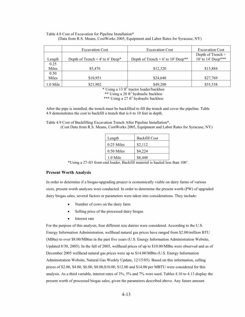
Table 4.8 Cost of Excavation for Pipeline Installation* (Data from R.S. Means, CostWorks 2005, Equipment and Labor Rates for Syracuse, NY)

Excavation Cost Excavation Cost Excavation Cost

Depth of Trench = 10' to 14' Deep*** Length Depth of Trench = 4' to 6' Deep* Depth of Trench = 6' to 10' Deep**

0.25 Miles $5,476 $12,320 $13,884 0.50

Miles $10,951 $24,640 $27,769 1.0 Mile $21,902 $49,280 $55,538

* Using a 13 ft3 tractor loader/backhoe ** Using a 20 ft3 hydraulic backhoe

*** Using a 27 ft3 hydraulic backhoe

After the pipe is installed, the trench must be backfilled to fill the trench and cover the pipeline. Table 4.9 demonstrates the cost to backfill a trench that is 6 to 10 feet in depth. Table 4.9 Cost of Backfilling Excavation Trench After Pipeline Installation*,

(Cost Data from R.S. Means, CostWorks 2005, Equipment and Labor Rates for Syracuse, NY)

Length Backfill Cost 0.25 Miles $2,112 0.50 Miles $4,224 1.0 Mile $8,448

*Using a 27-ft3 front-end loader, Backfill material is hauled less than 100’. Present Worth Analysis

In order to determine if a biogas-upgrading project is economically viable on dairy farms of various

sizes, present worth analyses were conducted. In order to determine the present worth (PW) of upgraded

dairy biogas sales, several factors or parameters were taken into considerations. They include:

• Number of cows on the dairy farm

• Selling price of the processed dairy biogas

• Interest rate

For the purpose of this analysis, four different size dairies were considered. According to the U.S.

Energy Information Administration, wellhead natural gas prices have ranged from $2.00/million BTU

(MBtu) to over $8.00/MBtus in the past five years (U.S. Energy Information Administration Website,

Updated 8/30, 2005). In the fall of 2005, wellhead prices of up to $10.00/MBtu were observed and as of

December 2005 wellhead natural gas prices were up to $14.00/MBtu (U.S. Energy Information

Administration Website, Natural Gas Weekly Update, 12/15/05). Based on this information, selling

prices of $2.00, $4.00, $6.00, $8.00,$10.00, $12.00 and $14.00 per MBTU were considered for this

analysis. As a third variable, interest rates of 3%, 5% and 7% were used. Tables 4.10 to 4.13 display the

present worth of processed biogas sales, given the parameters described above. Any future amount

4-13

compared to any present amount is known as the present worth (PW) and is calculated using Equation

4.2.

P= F (1+i)-n {Equation 4.2} From Equation 4.3, the PW of upgraded biogas sales is a function of the future amount of revenue

generated by biogas sales, interest rates and the number of compounding periods. To determine F,

biogas production, the methane content of the processed biogas and the amount of money the processed

biogas is sold for must be known. To determine F, the following steps were used:

• Determine the amount of biogas generated by the AD process. The volume of biogas produced

depends on the number of cows on the farm and the amount of biogas each produces.

• Once the amount of biogas generation is known, determine the amount of biogas that will be

used to heat the digester. The biogas that is used to heat the digester is subtracted from the total

amount of biogas available for processing.

• Next, the total amount of methane available for sale to the natural gas pipeline after the biogas

is processed must be determined. This takes into account any losses during processing.

• After the total methane available for sale is determined, the PW of the upgraded biogas can be

determined, depending on the selling price to the buyer.

We assumed that:

• Each cow produces 100 ft3 of biogas per day

• 60% of the biogas is methane and 90% of the methane is recovered from the upgrading

process.

• 25% of the biogas is used to heat the digester

An Excel spreadsheet was developed to calculate the present worth with the variables of cow numbers,

selling price for biogas and interest rates. The results from this analysis for farm sizes of 500, 1000,

3000, 5000 and 10000 cows are given in Figures 4.10 through 4.14.

4-14

Table 4.10. Present Worth Analysis for 500 Cow Dairy

Number of Cows Interest Rate Gas Selling Price PW of Processed Gas Sales 500 3% $2.00/MBtu $126,098 $4.00/MBtu $252,195 $6.00/MBtu $378,293 $8.00/MBtu $504,391 $10.00/MBtu $630,489 $12.00/MBtu $756,586 $14.00/MBtu $882,684 5% $2.00/MBtu $114,147 $4.00/MBtu $228,293 $6.00/MBtu $342,440 $8.00/MBtu $456,586 $10.00/MBtu $570,733 $12.00/MBtu $684,879 $14.00/MBtu $799,026 7% $2.00/MBtu $103,826 $4.00/MBtu $207,652 $6.00/MBtu $311,478 $8.00/MBtu $415,304 $10.00/MBtu $519,130 $12.00/MBtu $622,957 $14.00/MBtu $726,783

4-15

Table 4.11. Present Worth Analysis for 1,000 Cow Dairy

Number of Cows Interest Rate Gas Selling Price PW of Processed Gas Sales 1,000 3% $2.00/MBtu $252,195

$4.00/MBtu $504,391 $6.00/MBtu $756,586 $8.00/MBtu $1,008,782 $10.00/MBtu $1,260,977 $12.00/MBtu 1,513,173 $14.00/MBtu 1,765,368 5% $2.00/MBtu $228,293 $4.00/MBtu $456,586 $6.00/MBtu $684,879 $8.00/MBtu $913,172 $10.00/MBtu $1,141,465 $12.00/MBtu 1,369,759 $14.00/MBtu 1,598,052 7% $2.00/MBtu $207,652 $4.00/MBtu $415,304 $6.00/MBtu $622,957 $8.00/MBtu $830,609 $10.00/MBtu $1,038,261 $12.00/MBtu 1,245,913 $14.00/MBtu 1,453,565

4-16

Table 4.12. Present Worth Analysis for 3,000 Cow Dairy

Number of Cows Interest Rate Gas Selling Price PW of Processed Gas Sales 3,000 3% $2.00/MBtu $756,586

$4.00/MBtu $1,513,173 $6.00/MBtu 2,269,759 $8.00/MBtu 3,026,345 $10.00/MBtu $3,782,932 $12.00/MBtu $4,539,518 $14.00/MBtu $5,296,104 5% $2.00/MBtu 684,879 $4.00/MBtu 1,369,759 $6.00/MBtu 2,054,638 $8.00/MBtu 2,739,517 $10.00/MBtu $3,424,396 $12.00/MBtu $4,109,276 $14.00/MBtu $4,794,155 7% $2.00/MBtu 622,957 $4.00/MBtu 1,245,913 $6.00/MBtu 1,868,870 $8.00/MBtu 2,491,826 $10.00/MBtu $3,114,783 $12.00/MBtu $3,737,739 $14.00/MBtu $4,360,696

4-17

Table 4.13. Present Worth Analysis for 5,000 Cow Dairy

Number of Cows Interest Rate Gas Selling Price PW of Processed Gas Sales 5,000 3% $2.00/MBtu 1,260,977 $4.00/MBtu 2,521,954 $6.00/MBtu 3,782,932 $8.00/MBtu 5,043,909 $10.00/MBtu $6,304,886 $12.00/MBtu 7,565,863 $14.00/MBtu 8,826,841 5% $2.00/MBtu 1,141,465 $4.00/MBtu 2,282,931 $6.00/MBtu 3,424,396 $8.00/MBtu 4,565,862 $10.00/MBtu $5,707,327 $12.00/MBtu 6,848,793 $14.00/MBtu 7,990,258 7% $2.00/MBtu 1,038,261 $4.00/MBtu $2,076,522 $6.00/MBtu $3,114,783 $8.00/MBtu $4,153,044 $10.00/MBtu $5,191,072 $12.00/MBtu 6,229,566 $14.00/MBtu 7,267,827

4-18

Table 4.14. Present Worth Analysis for 10,000 Cow Dairy

Number of Cows Interest Rate Gas Selling Price PW of Processed Gas Sales 10,000 3% $2.00/MBtu $2,521,954 $4.00/MBtu $5,043,909 $6.00/MBtu $7,565,863 $8.00/MBtu $10,087,818 $10.00/MBtu $12,609,772 $12.00/MBtu $15,131,727 $14.00/MBtu $17,653,681 5% $2.00/MBtu $2,282,931 $4.00/MBtu $4,565,862 $6.00/MBtu $6,848,793 $8.00/MBtu $9,131,724 $10.00/MBtu $11,414,655 $12.00/MBtu $13,697,586 $14.00/MBtu $15,980,517 7% $2.00/MBtu $2,076,522 $4.00/MBtu $4,153,044 $6.00/MBtu $6,229,566 $8.00/MBtu $8,306,088 $10.00/MBtu $10,382,609 $12.00/MBtu $12,459,131 $14.00/MBtu $14,535,653

Financial Viability of Processing Biogas to Natural Gas Quality on Dairy Farms of Various Sizes

In New York State (NYS), most dairies have 500 cows or less. However, as the shift from smaller

dairies to CAFOs continues, the number of large dairies is likely to increase in coming years. Also,

current research suggests that centralized digesters may be feasible, allowing manure from multiple

farms to be digested at one centralized location. For further information, see Centralized Anaerobic

Digestion Options for Groups of Dairy Farms (Bothi and Aldrich, May, 2005) and Feasibility of a

Central Anaerobic Digester for Ten Dairy Farms in Salem, NY (Bothi and Aldrich, June 2005).

In other parts of the country, such as California and Illinois, larger dairies with 3,000 to 10,000 cows

exist. In several states, like New York, where smaller dairies exist in close proximity to each other, a

community digester that accepts waste from several farms and possibly food processing plants may be

4-19

4-20

an option to make processing biogas to natural gas quality feasible from a financial standpoint.

Additionally, NYS is following the nation-wide trend toward larger, more efficient dairy operations.

In 2003, the Cayuga County Soil and Water Conservation District (SWCD) proposed to build a

community digester in Auburn, NY. The feasibility study for this project was partially funded by

NYSERDA. The plug flow digester is sized to treat an equivalent herd of 3,500 animals, with the

digester influent containing dairy manure and other organic wastes, such as food waste and food

processing wastes. The proposed digester will treat manure from 2,800 cows, approximately 28% of

animals in the area and 21,200 tons of food waste per year. This will result in the production of

350,000f3/biogas per day, assuming the equivalent herd of 3,500 cows (biogas produced from dairy

manure and food waste digestion) produces 100f3/biogas daily. To date, this project seeking funds and

has not begun construction, but demonstrates the potential that community digesters have to treat large

amounts of waste while producing significant quantities of biogas. This project, as an example,

demonstrates that farmers, communities and government agencies are interested in pursuing community

digesters in New York State.

In additions, a project being developed by Global Common will collect manure from about 7,000 dairy

cows at four farms in Cayuga County, NY. The manure will be transported to a centralized digester by

pipeline or trucks. In order to increase biogas output and quality, the digesters will also utilize organic

wastes from food processing plants. The biogas that is generated will be used to fire a co-generation

system that will provide electricity to a nearby prison.

For the purpose of this analysis, five different size dairies are considered (500, 1,000, 3,000, 5,000 and

10,000 cows. We assume 90% of the biogas that is generated during the digestion process is captured

for use and that 25% of the biogas is used to heat the digester. The present worth income (or loss) of

processed, high Btu biogas sales over a ten year period for the five different size dairies and considering

the estimated gas processing and O&M costs to transform raw dairy biogas into natural gas quality gas

as is given in Table 4.3 and Table 4.4, we show in Tables 4.15 to 4.19 a summary of the PW income of

upgraded biogas sales, taking into account capital costs to build the gas processing system and O&M

costs to run the system. The present worth income (or loss) is calculated using Equation 4.3.

PW of Income = PW of Revenue from Gas Sales - PW of Capital Costs – PW of O& M Costs {Equation 4.3}

These cost estimates do not include the installation of additional pipeline to bring the processed biogas

to the main natural gas pipeline. Here, it is assumed that the biogas production and processing site is

located adjacent to the natural gas pipeline that it will be injected into.

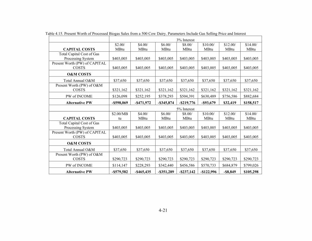
Table 4.15. Present Worth of Processed Biogas Sales from a 500 Cow Dairy. Parameters Include Gas Selling Price and Interest 3% Interest

$2.00/ $4.00/ $6.00/ $8.00/ $10.00/ $12.00/ $14.00/ CAPITAL COSTS MBtu MBtu MBtu MBtu MBtu MBtu MBtu

Total Capital Cost of Gas Processing System $403,005 $403,005 $403,005 $403,005 $403,005 $403,005 $403,005

Present Worth (PW) of CAPITAL COSTS $403,005 $403,005 $403,005 $403,005 $403,005 $403,005 $403,005

O&M COSTS Total Annual O&M $37,650 $37,650 $37,650 $37,650 $37,650 $37,650 $37,650

Present Worth (PW) of O&M COSTS $321,162 $321,162 $321,162 $321,162 $321,162 $321,162 $321,162

PW of INCOME $126,098 $252,195 $378,293 $504,391 $630,489 $756,586 $882,684 Alternative PW -$598,069 -$471,972 -$345,874 -$219,776 -$93,679 $32,419 $158,517

5% Interest $2.00/MB

tu $4.00/ $6.00/ $8.00/ $10.00/ $12.00/ $14.00/

CAPITAL COSTS MBtu MBtu MBtu MBtu MBtu MBtu Total Capital Cost of Gas

Processing System $403,005 $403,005 $403,005 $403,005 $403,005 $403,005 $403,005 Present Worth (PW) of CAPITAL

COSTS $403,005 $403,005 $403,005 $403,005 $403,005 $403,005 $403,005 O&M COSTS

Total Annual O&M $37,650 $37,650 $37,650 $37,650 $37,650 $37,650 $37,650 Present Worth (PW) of O&M

COSTS $290,723 $290,723 $290,723 $290,723 $290,723 $290,723 $290,723 PW of INCOME $114,147 $228,293 $342,440 $456,586 $570,733 $684,879 $799,026 Alternative PW -$579,582 -$465,435 -$351,289 -$237,142 -$122,996 -$8,849 $105,298

4-21

4-22

Table 4.15 (Continued) 7% Interest

CAPITAL COSTS $2.00/ MBtu

$4.00/ MBtu

$6.00/ MBtu

$8.00/ MBtu

$10.00/ MBtu

$12.00/ MBtu

$14.00/ MBtu

Total Capital Cost of Gas Processing System $403,005 $403,005 $403,005 $403,005 $403,005 $403,005 $403,005

Present Worth (PW) of CAPITAL COSTS $403,005 $403,005 $403,005 $403,005 $403,005 $403,005 $403,005

O&M COSTS Total Annual O&M $37,650 $37,650 $37,650 $37,650 $37,650 $37,650 $37,650

Present Worth (PW) of O&M COSTS $264,438 $264,438 $264,438 $264,438 $264,438 $264,438 $264,438

PW of INCOME $103,826 $207,652 $311,478 $415,304 $519,130 $622,957 $726,783 Alternative PW -$563,617 -$459,791 -$355,965 -$252,138 -$148,312 -$44,486 $59,340

Table 4.16. Present Worth of Processed Biogas Sales from a 1,000 Cow Dairy. Parameters Include Gas Selling Price and Interest 3% Interest

CAPITAL COSTS $2.00/ MBtu

$4.00/ MBtu

$6.00/ MBtu

$8.00/ MBtu

$10.00/ MBtu

$12.00/ MBtu

$14.00/ MBtu

Total Capital Cost of Gas Processing System $403,005 $403,005 $403,005 $403,005 $403,005 $403,005 $403,005

Present Worth (PW) of CAPITAL COSTS $403,005 $403,005 $403,005 $403,005 $403,005 $403,005 $403,005

O&M COSTS Total Annual O&M $37,650 $37,650 $37,650 $37,650 $37,650 $37,650 $37,650

Present Worth (PW) of O&M COSTS $321,162 $321,162 $321,162 $321,162 $321,162 $321,162 $321,162

PW of INCOME $252,195 $504,391 $756,586 $1,008,78

2 $1,260,97

7 1,513,173 1,765,368 Alternative PW -$471,972 -$219,776 $32,419 $284,615 $536,810 $789,006 $1,041,201

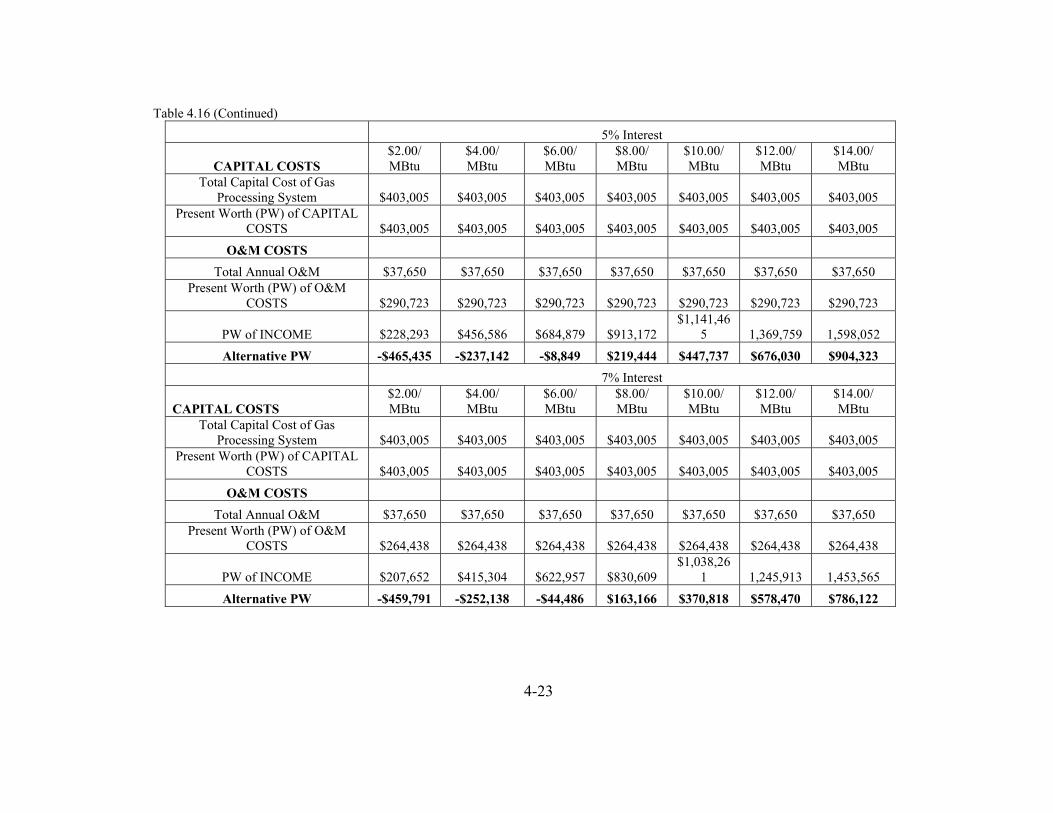
4-23

Table 4.16 (Continued) 5% Interest

CAPITAL COSTS $2.00/ MBtu

$4.00/ MBtu

$6.00/ MBtu

$8.00/ MBtu

$10.00/ MBtu

$12.00/ MBtu

$14.00/ MBtu

Total Capital Cost of Gas Processing System $403,005 $403,005 $403,005 $403,005 $403,005 $403,005 $403,005

Present Worth (PW) of CAPITAL COSTS $403,005 $403,005 $403,005 $403,005 $403,005 $403,005 $403,005

O&M COSTS Total Annual O&M $37,650 $37,650 $37,650 $37,650 $37,650 $37,650 $37,650

Present Worth (PW) of O&M COSTS $290,723 $290,723 $290,723 $290,723 $290,723 $290,723 $290,723

PW of INCOME $228,293 $456,586 $684,879 $913,172 $1,141,46

5 1,369,759 1,598,052 Alternative PW -$465,435 -$237,142 -$8,849 $219,444 $447,737 $676,030 $904,323

7% Interest

CAPITAL COSTS $2.00/ MBtu

$4.00/ MBtu

$6.00/ MBtu

$8.00/ MBtu

$10.00/ MBtu

$12.00/ MBtu

$14.00/ MBtu

Total Capital Cost of Gas Processing System $403,005 $403,005 $403,005 $403,005 $403,005 $403,005 $403,005

Present Worth (PW) of CAPITAL COSTS $403,005 $403,005 $403,005 $403,005 $403,005 $403,005 $403,005

O&M COSTS Total Annual O&M $37,650 $37,650 $37,650 $37,650 $37,650 $37,650 $37,650

Present Worth (PW) of O&M COSTS $264,438 $264,438 $264,438 $264,438 $264,438 $264,438 $264,438

PW of INCOME $207,652 $415,304 $622,957 $830,609 $1,038,26

1 1,245,913 1,453,565 Alternative PW -$459,791 -$252,138 -$44,486 $163,166 $370,818 $578,470 $786,122

4-24

Table 4.17. Present Worth of Processed Biogas Sales from a 3,000 Cow Dairy. Parameters Include Gas Selling Price and Interest

3% Interest

CAPITAL COSTS $2.00/ MBtu

$4.00/ MBtu

$6.00/ MBtu

$8.00/ MBtu

$10.00/ MBtu

$12.00/ MBtu

$14.00/ MBtu

Total Capital Cost of Gas Processing System $799,075 $799,075 $799,075 $799,075 $799,075 $799,075 $799,075

Present Worth (PW) of CAPITAL COSTS $799,075 $799,075 $799,075 $799,075 $799,075 $799,075 $799,075

O&M COSTS Total Annual O&M $75,150 $75,150 $75,150 $75,150 $75,150 $75,150 $75,150

Present Worth (PW) of O&M COSTS $641,045 $641,045 $641,045 $641,045 $641,045 $641,045 $641,045

PW of INCOME $756,586 $1,513,17

3 $2,269,75

9 $3,026,345 $3,782,932 $4,539,518 $5,296,104 Alternative PW -$683,534 $73,053 $829,639 $1,586,226 $2,342,812 $3,099,398 $3,855,985

5% Interest

CAPITAL COSTS $2.00/ MBtu

$4.00/ MBtu

$6.00/ MBtu

$8.00/ MBtu

$10.00/ MBtu

$12.00/ MBtu

$14.00/ MBtu

Total Capital Cost of Gas Processing System $799,075 $799,075 $799,075 $799,075 $799,075 $799,075 $799,075

Present Worth (PW) of CAPITAL COSTS $799,075 $799,075 $799,075 $799,075 $799,075 $799,075 $799,075

O&M COSTS Total Annual O&M $75,150 $75,150 $75,150 $75,150 $75,150 $75,150 $75,150

Present Worth (PW) of O&M COSTS $580,288 $580,288 $580,288 $580,288 $580,288 $580,288 $580,288

PW of INCOME $684,879 $1,369,75

9 $2,054,63

8 $2,739,517 $3,424,396 $4,109,276 $4,794,155 Alternative PW -$694,484 -$9,604 $675,275 $1,360,154 $2,045,033 $2,729,912 $3,414,792

4-25

Table 4.17 (Continued) 7% Interest

CAPITAL COSTS $2.00/ MBtu

$4.00/ MBtu

$6.00/ MBtu

$8.00/ MBtu

$10.00/ MBtu

$12.00/ MBtu

$14.00/ MBtu

Total Capital Cost of Gas Processing System $799,075 $799,075 $799,075 $799,075 $799,075 $799,075 $799,075

Present Worth (PW) of CAPITAL COSTS $799,075 $799,075 $799,075 $799,075 $799,075 $799,075 $799,075

O&M COSTS Total Annual O&M $75,150 $75,150 $75,150 $75,150 $75,150 $75,150 $75,150

Present Worth (PW) of O&M COSTS $527,822 $527,822 $527,822 $527,822 $527,822 $527,822 $527,822

PW of INCOME $622,957 $1,245,91

3 $1,868,87

0 $2,491,826 $3,114,783 $3,737,739 $4,360,696 Alternative PW -$703,940 -$80,984 $541,973 $1,164,929 $1,787,886 $2,410,842 $3,033,799

Table 4.18. Present Worth of Processed Biogas Sales from a 5,000 Cow Dairy.Parameters Include Gas Selling Price and Interest 3% Interest

CAPITAL COSTS $2.00/ MBtu

$4.00/ MBtu

$6.00/ MBtu

$8.00/ MBtu

$10.00/ MBtu

$12.00/ MBtu

$14.00/ MBtu

Total Capital Cost of Gas Processing System $1,519,675 $1,519,675 $1,519,675 $1,519,675 $1,519,675 $1,519,675 $1,519,675

Present Worth (PW) of CAPITAL COSTS $1,519,675 $1,519,675 $1,519,675 $1,519,675 $1,519,675 $1,519,675 $1,519,675

O&M COSTS Total Annual O&M $108,600 $108,600 $108,600 $108,600 $108,600 $108,600 $108,600

Present Worth (PW) of O&M COSTS $926,380 $926,380 $926,380 $926,380 $926,380 $926,380 $926,380

PW of INCOME $1,260,977 $2,521,954 $3,782,932 $5,043,909 $6,304,886 7,565,863 8,826,841 Alternative PW -$1,185,078 $75,899 $1,336,877 $2,597,854 $3,858,831 $5,119,808 $6,380,786

4-26

Table 4.18 (Continued) 5% Interest

CAPITAL COSTS $2.00/ MBtu

$4.00/ MBtu

$6.00/ MBtu

$8.00/ MBtu

$10.00/ MBtu

$12.00/ MBtu

$14.00/ MBtu

Total Capital Cost of Gas Processing System $1,519,675 $1,519,675 $1,519,675 $1,519,675 $1,519,675 $1,519,675 $1,519,675

Present Worth (PW) of CAPITAL COSTS $1,519,675 $1,519,675 $1,519,675 $1,519,675 $1,519,675 $1,519,675 $1,519,675

O&M COSTS Total Annual O&M $108,600 $108,600 $108,600 $108,600 $108,600 $108,600 $108,600

Present Worth (PW) of O&M COSTS $838,580 $838,580 $838,580 $838,580 $838,580 $838,580 $838,580

PW of INCOME $1,141,465 $2,282,931 $3,424,396 $4,565,862 $5,707,327 6,848,793 7,990,258 Alternative PW -$1,216,790 -$75,324 $1,066,141 $2,207,607 $3,349,072 $4,490,537 $5,632,003

7% Interest

CAPITAL COSTS $2.00/ MBtu

$4.00/ MBtu

$6.00/ MBtu

$8.00/ MBtu

$10.00/ MBtu

$12.00/ MBtu

$14.00/ MBtu

Total Capital Cost of Gas Processing System $1,519,675 $1,519,675 $1,519,675 $1,519,675 $1,519,675 $1,519,675 $1,519,675

Present Worth (PW) of CAPITAL COSTS $1,519,675 $1,519,675 $1,519,675 $1,519,675 $1,519,675 $1,519,675 $1,519,675

O&M COSTS Total Annual O&M $108,600 $108,600 $108,600 $108,600 $108,600 $108,600 $108,600

Present Worth (PW) of O&M COSTS $762,761 $762,761 $762,761 $762,761 $762,761 $762,761 $762,761

PW of INCOME $1,038,261 $2,076,522 $3,114,783 $4,153,044 $5,191,072 6,229,566 7,267,827 Alternative PW -$1,244,175 -$205,914 $832,347 $1,870,608 $2,908,636 $3,947,130 $4,985,391

Table 4.19. Present Worth of Processed Biogas Sales from a 10,000 Cow Dairy. Parameters Include Gas Selling Price and Interest

3% Interest $2.00/ $4.00/ $6.00/ $8.00/ $10.00/ $12.00/ $14.00/

CAPITAL COSTS MBtu MBtu MBtu MBtu MBtu MBtu MBtu Total Capital Cost of Gas

Processing System $2,397,400 $2,397,400 $2,397,400 $2,397,400 $2,165,400 $2,397,400 $2,165,400 Present Worth (PW) of CAPITAL

COSTS $2,397,400 $2,397,400 $2,397,400 $2,397,400 $2,165,400 $2,397,400 $2,165,400 O&M COSTS

Total Annual O&M $204,400 $204,400 $204,400 $204,400 $180,600 $204,400 $180,600 Present Worth (PW) of O&M

COSTS $1,743,573 $1,743,573 $1,743,573 $1,743,573 $1,540,555 $1,743,573 $1,540,555 PW of INCOME $2,521,954 $5,043,909 $7,565,863 $10,087,818 $12,609,772 $15,131,727 $17,653,681 Alternative PW -$1,184,001 $1,337,954 $3,859,908 $6,381,863 $8,903,817 $11,425,772 $13,947,727

5% Interest $2.00/ $4.00/ $6.00/ $8.00/ $10.00/ $12.00/ $14.00/

CAPITAL COSTS MBtu MBtu MBtu MBtu MBtu MBtu MBtu Total Capital Cost of Gas

Processing System $2,397,400 $2,397,400 $2,397,400 $2,397,400 $2,165,400 $2,397,400 $2,165,400 Present Worth (PW) of CAPITAL

COSTS $2,397,400 $2,397,400 $2,397,400 $2,397,400 $2,165,400 $2,397,400 $2,165,400 O&M COSTS

Total Annual O&M $204,400 $204,400 $204,400 $204,400 $180,600 $204,400 $180,600 Present Worth (PW) of O&M

COSTS $1,578,323 $1,578,323 $1,578,323 $1,578,323 $1,394,545 $1,578,323 $1,394,545 PW of INCOME $2,282,931 $4,565,862 $6,848,793 $9,131,724 $11,414,655 $13,697,586 $15,980,517 Alternative PW -$1,277,014 $1,005,917 $3,288,848 $5,571,779 $7,854,710 $10,137,640 $12,420,571

4-27

4-28

Table 4.19 (Continued)

7% Interest

CAPITAL COSTS $2.00/MBtu $4.00/MBtu $6.00/MBtu $8.00/MBtu $10.00/Mbut $12.00/MBt

u $14.00//M Total Capital Cost of Gas

Processing System $2,397,400 $2,397,400 $2,397,400 $2,397,400 $2,165,400 $2,397,400 $2,165,400 Present Worth (PW) of CAPITAL

COSTS $2,397,400 $2,397,400 $2,397,400 $2,397,400 $2,165,400 $2,397,400 $2,165,400 O&M COSTS

Total Annual O&M $204,400 $204,400 $204,400 $204,400 $180,600 $204,400 $180,600 Present Worth (PW) of O&M

COSTS $1,435,620 $1,435,620 $1,435,620 $1,435,620 $1,268,459 $1,435,620 $1,268,459 PW of INCOME $2,076,522 $4,153,044 $6,229,566 $8,306,088 $10,382,609 $12,459,131 $14,535,653

$11,101,794 Alternative PW -$1,357,337 $719,185 $2,795,707 $4,872,229 $6,948,750 $9,025,272

4-29

Financial Viability of Processing Biogas to Natural Gas Quality on Dairy Farms of Various Sizes with Addition of Pipeline Installation Realistically, it is unlikely that the biogas production and processing site will be located right next to

the natural gas pipeline. Therefore, pipeline installation costs can play an important part in determining

the economic viability of the project. Tables 4.20 to 4.24 show the PW analysis of selling upgraded

biogas with ¼ mile, ½ mile and 1 mile pipeline installations for the five dairies. The PW of processed

biogas sales was determined by Equation 4.4.

PW of Income = PW of Revenue from Gas Sales - PW of Capital Costs – PW of O& M Costs – Cost of

Pipeline Installation {Equation 4.4}

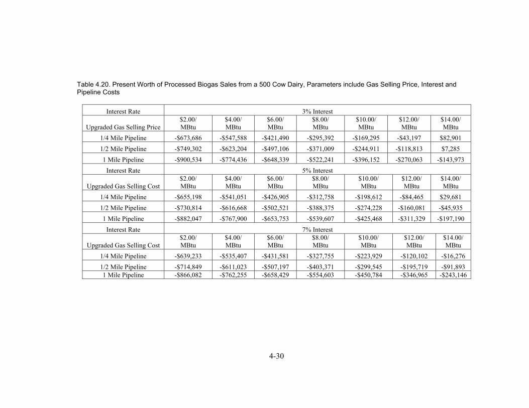
Table 4.20. Present Worth of Processed Biogas Sales from a 500 Cow Dairy, Parameters include Gas Selling Price, Interest and Pipeline Costs

Interest Rate 3% Interest $2.00/ $4.00/ $6.00/ $8.00/ $10.00/ $12.00/ $14.00/ MBtu MBtu MBtu MBtu MBtu MBtu MBtu Upgraded Gas Selling Price

1/4 Mile Pipeline -$673,686 -$547,588 -$421,490 -$295,392 -$169,295 -$43,197 $82,901 1/2 Mile Pipeline -$749,302 -$623,204 -$497,106 -$371,009 -$244,911 -$118,813 $7,285 1 Mile Pipeline -$900,534 -$774,436 -$648,339 -$522,241 -$396,152 -$270,063 -$143,973

Interest Rate 5% Interest $2.00/ $4.00/ $6.00/ $8.00/ $10.00/ $12.00/ $14.00/ MBtu MBtu MBtu MBtu MBtu MBtu MBtu Upgraded Gas Selling Cost

1/4 Mile Pipeline -$655,198 -$541,051 -$426,905 -$312,758 -$198,612 -$84,465 $29,681 1/2 Mile Pipeline -$730,814 -$616,668 -$502,521 -$388,375 -$274,228 -$160,081 -$45,935 1 Mile Pipeline -$882,047 -$767,900 -$653,753 -$539,607 -$425,468 -$311,329 -$197,190

Interest Rate 7% Interest $2.00/ $4.00/ $6.00/ $8.00/ $10.00/ $12.00/ $14.00/ MBtu MBtu MBtu MBtu MBtu MBtu MBtu Upgraded Gas Selling Cost

1/4 Mile Pipeline -$639,233 -$535,407 -$431,581 -$327,755 -$223,929 -$120,102 -$16,276 1/2 Mile Pipeline -$714,849 -$611,023 -$507,197 -$403,371 -$299,545 -$195,719 -$91,893 1 Mile Pipeline -$866,082 -$762,255

-$658,429 -$554,603 -$450,784 -$346,965 -$243,146

4-30

Table 4.21. Present Worth of Processed Biogas Sales from a 1,000 Cow Dairy, Parameters include Gas Selling Price, Interest and Pipeline Costs.

Interest Rate 3% Interest $10.00/MBtu Upgraded Gas Selling Price $2.00/MBtu $4.00/MBtu $6.00/MBtu $8.00/MBtu $12.00/MBtu $14.00/MBtu

$461,194 1/4 Mile Pipeline -$547,588 -$295,392 -$43,197 $208,998 $713,389 $965,585 $385,577 1/2 Mile Pipeline -$623,204 -$371,009 -$118,813 $133,382 $637,773 $889,969 $234,337 1 Mile Pipeline -$814,036 -$561,841 -$309,646 -$57,450 $486,524 $738,711

Interest Rate 5% Interest $10.00/MBtu Upgraded Gas Selling Cost $2.00/MBtu $4.00/MBtu $6.00/MBtu $8.00/MBtu $12.00/MBtu $14.00//M

$372,120 1/4 Mile Pipeline -$541,051 -$312,758 -$84,465 $143,828 $600,414 $828,707 $296,504 1/2 Mile Pipeline -$616,668 -$388,375 -$160,081 $68,212 $524,798 $753,091 $145,264 1 Mile Pipeline -$807,500 -$579,207 -$350,914 -$122,621 $373,550 $601,835

Interest Rate 7% Interest $10.00/MBtu Upgraded Gas Selling Cost $2.00/MBtu $4.00/MBtu $6.00/MBtu $8.00/MBtu $12.00/MBtu $14.00//M

$295,202 1/4 Mile Pipeline -$535,407 -$327,755 -$120,102 $87,550 $502,854 $710,506 $219,586 1/2 Mile Pipeline -$611,023 -$403,371 -$195,719 $11,934 $427,238 $634,890

1 Mile Pipeline -$801,855 -$594,203

4-31

-$386,551 -$178,899 $68,346 $275,991 $483,637

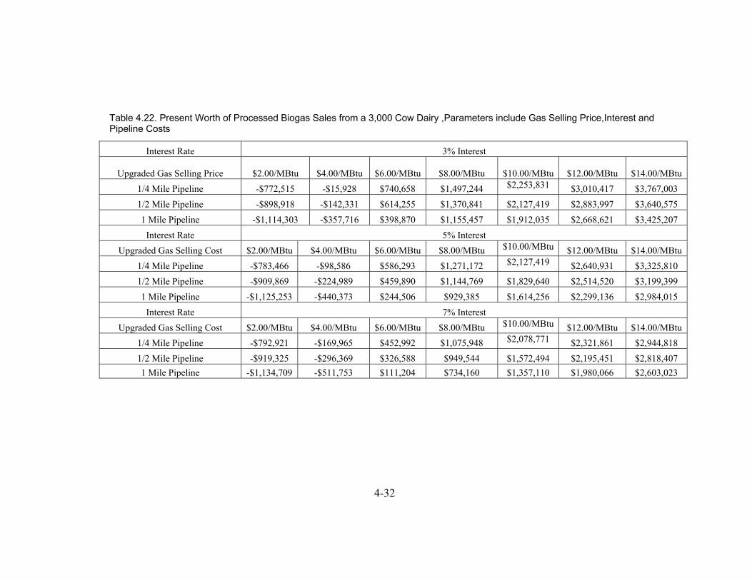
Table 4.22. Present Worth of Processed Biogas Sales from a 3,000 Cow Dairy ,Parameters include Gas Selling Price,Interest and Pipeline Costs

Interest Rate 3% Interest

Upgraded Gas Selling Price $2.00/MBtu $4.00/MBtu $6.00/MBtu $8.00/MBtu $10.00/MBtu $12.00/MBtu $14.00/MBtu $2,253,831 1/4 Mile Pipeline -$772,515 -$15,928 $740,658 $1,497,244 $3,010,417 $3,767,003

1/2 Mile Pipeline -$898,918 -$142,331 $614,255 $1,370,841 $2,127,419 $2,883,997 $3,640,575 1 Mile Pipeline -$1,114,303 -$357,716 $398,870 $1,155,457 $1,912,035 $2,668,621 $3,425,207

Interest Rate 5% Interest

4-32

Upgraded Gas Selling Cost $2.00/MBtu $4.00/MBtu $6.00/MBtu $8.00/MBtu $10.00/MBtu $12.00/MBtu $14.00/MBtu $2,127,419 1/4 Mile Pipeline -$783,466 -$98,586 $586,293 $1,271,172 $2,640,931 $3,325,810

1/2 Mile Pipeline -$909,869 -$224,989 $459,890 $1,144,769 $1,829,640 $2,514,520 $3,199,399 1 Mile Pipeline -$1,125,253 -$440,373 $244,506 $929,385 $1,614,256 $2,299,136 $2,984,015

Interest Rate 7% Interest Upgraded Gas Selling Cost $2.00/MBtu $4.00/MBtu $6.00/MBtu $8.00/MBtu $10.00/MBtu $12.00/MBtu $14.00/MBtu

$2,078,771 1/4 Mile Pipeline -$792,921 -$169,965 $452,992 $1,075,948 $2,321,861 $2,944,818 1/2 Mile Pipeline -$919,325 -$296,369 $326,588 $949,544 $1,572,494 $2,195,451 $2,818,407 1 Mile Pipeline -$1,134,709 -$511,753 $111,204 $734,160 $1,357,110 $1,980,066 $2,603,023

Table 4.23. Present Worth of Processed Biogas Sales from a 5,000 Cow Dairy, Parameters include Gas Selling Price, Interest and Pipeline Costs

Interest Rate 3% Interest

Upgraded Gas Selling Price $2.00/MBtu $4.00/MBtu $6.00/MBtu $8.00/MBtu $10.00/MBtu $12.00/MBtu $14.00/MBtu $3,751,139 1/4 Mile Pipeline -$1,292,770 -$31,793 $1,229,185 $2,490,162 $5,012,116 $6,273,093 $3,241,379 1/2 Mile Pipeline -$1,449,111 -$188,134 $1,072,844 $2,333,821 $4,855,775 $6,116,753 $2,800,944 1 Mile Pipeline -$1,770,881 -$509,904 $751,074 $2,012,051 $4,533,997 $5,794,966

Interest Rate 5% Interest

Upgraded Gas Selling Cost $2.00/MBtu $4.00/MBtu $6.00/MBtu $8.00/MBtu $10.00/MBtu $12.00/MBtu $14.00/MBtu $3,594,798 1/4 Mile Pipeline -$1,324,483 -$183,017 $958,448 $2,099,914 $4,382,845 $5,524,311 $3,085,039 1/2 Mile Pipeline -$1,480,823 -$339,357 $802,108 $1,943,574 $4,226,504 $5,367,970 $2,644,603 1 Mile Pipeline -$1,802,593 -$661,127 $480,338 $1,621,804 $3,904,727 $5,046,185

Interest Rate 7% Interest

Upgraded Gas Selling Cost $2.00/MBtu $4.00/MBtu $6.00/MBtu $8.00/MBtu $10.00/MBtu $12.00/MBtu $14.00/MBtu $3,273,028 1/4 Mile Pipeline -$1,351,867 -$313,606 $724,655 $1,762,916 $3,839,437 $4,877,698

$2,763,269 1/2 Mile Pipeline -$1,508,208 -$469,947 $568,314 $1,606,575 $3,683,097 $4,721,358 $2,322,826 1 Mile Pipeline -$1,829,978 -$791,717

4-33

$246,544 $1,284,805 $3,361,313 $4,399,567

4-34

Table 4.24. Present Worth of Processed Biogas Sales from a 10,000 Cow Dairy. Parameters include Gas Selling Price, Interest and Pipeline Costs

Interest Rate 3% Interest

Upgraded Gas Selling Price $2.00/MBtu $4.00/MBtu $6.00/MBtu $8.00/MBtu

$10.00/MBtu $12.00/MBtu $14.00/MBtu 1/4 Mile Pipeline -$1,765,470 $756,485 $3,278,439 $5,800,394 $8,757,367 $11,279,321 $13,801,276 1/2 Mile Pipeline -$1,911,921 $610,034 $3,131,988 $5,653,943 $7,708,259 $11,132,871 $13,654,825 1 Mile Pipeline -$2,259,351 $262,604 $2,784,558 $5,306,513 $6,802,299 $10,350,404 $12,872,350

Interest Rate 5% Interest

Upgraded Gas Selling Cost $2.00/MBtu $4.00/MBtu $6.00/MBtu $8.00/MBtu

$10.00/MBtu $12.00/MBtu $14.00/MBtu 1/4 Mile Pipeline -$1,839,242 $443,689 $2,726,620 $5,009,551 $8,610,916 $9,991,190 $12,274,120 1/2 Mile Pipeline -$1,985,693 $297,238 $2,580,169 $4,863,100 $7,561,808 $9,844,739 $12,127,670 1 Mile Pipeline -$2,333,124 -$50,193 $2,232,738 $4,515,669 $6,655,849 $9,081,516 $11,364,439

Interest Rate 7% Interest

Upgraded Gas Selling Cost $2.00/MBtu $4.00/MBtu $6.00/MBtu $8.00/MBtu

$10.00/MBtu $12.00/MBtu $14.00/MBtu 1/4 Mile Pipeline -$1,902,949 $173,573 $2,250,095 $4,326,617 $7,828,458 $8,878,822 $10,955,344 1/2 Mile Pipeline -$2,049,399 $27,123 $2,103,645 $4,180,167 $6,798,593 $8,732,371 $10,808,893

$7,985,765 $10,062,280 $5,909,250 $3,832,736 $1,756,214 -$320,308 -$2,396,830 1 Mile Pipeline

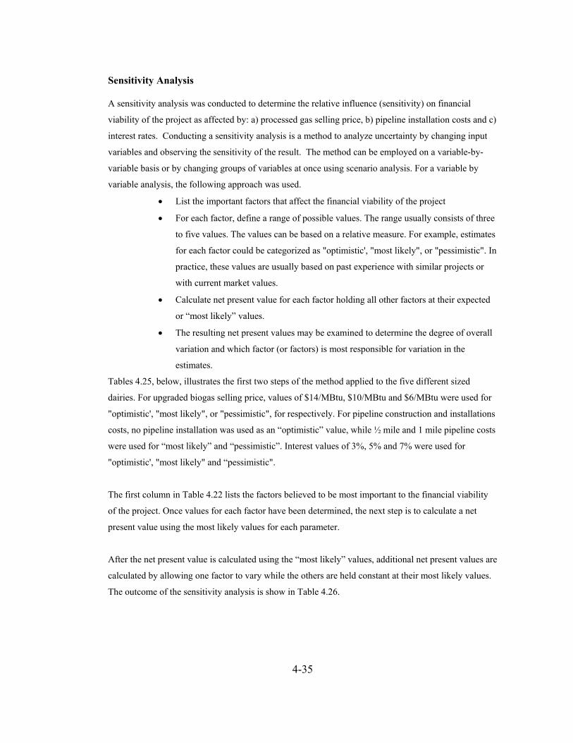
4-35

Sensitivity Analysis

A sensitivity analysis was conducted to determine the relative influence (sensitivity) on financial

viability of the project as affected by: a) processed gas selling price, b) pipeline installation costs and c)

interest rates. Conducting a sensitivity analysis is a method to analyze uncertainty by changing input

variables and observing the sensitivity of the result. The method can be employed on a variable-by-

variable basis or by changing groups of variables at once using scenario analysis. For a variable by

variable analysis, the following approach was used.

• List the important factors that affect the financial viability of the project

• For each factor, define a range of possible values. The range usually consists of three

to five values. The values can be based on a relative measure. For example, estimates

for each factor could be categorized as "optimistic', "most likely", or "pessimistic". In

practice, these values are usually based on past experience with similar projects or

with current market values.

• Calculate net present value for each factor holding all other factors at their expected

or “most likely” values.

• The resulting net present values may be examined to determine the degree of overall

variation and which factor (or factors) is most responsible for variation in the

estimates.

Tables 4.25, below, illustrates the first two steps of the method applied to the five different sized

dairies. For upgraded biogas selling price, values of $14/MBtu, $10/MBtu and $6/MBtu were used for

"optimistic', "most likely", or "pessimistic", for respectively. For pipeline construction and installations

costs, no pipeline installation was used as an “optimistic” value, while ½ mile and 1 mile pipeline costs

were used for “most likely” and “pessimistic”. Interest values of 3%, 5% and 7% were used for

"optimistic', "most likely" and “pessimistic".

The first column in Table 4.22 lists the factors believed to be most important to the financial viability

of the project. Once values for each factor have been determined, the next step is to calculate a net

present value using the most likely values for each parameter.

After the net present value is calculated using the “most likely” values, additional net present values are

calculated by allowing one factor to vary while the others are held constant at their most likely values.

The outcome of the sensitivity analysis is show in Table 4.26.

4-36

Table 4.25.Parameters Used in the Three Parameter Sensitivity Analysis for Five Different Size Dairies

Factor Optimistic Most Likely Pessimistic 500 Cows

Upgraded Gas Selling Price ($/Mbtu) 14 10 6 Pipeline Costs $0 $151,232 $302,465 Interest Rate 3% 5% 7%

1,000 Cows Upgraded Gas Selling Price ($/Mbtu) 14 10 6

Pipeline Costs $0 $151,232 $302,465 Interest Rate 3% 5% 7%

3,000 Cow Upgraded Gas Selling Price 14 10 6

Pipeline Costs $0 $215,384 $430,769 Interest Rate 3% 5% 7%

5,000 Cows Upgraded Gas Selling Price 14 10 6

Pipeline Costs $0 $264,033 $585,803 Interest Rate 3% 5% 7%

10,000 Cows Upgraded Gas Selling Price 14 10 6

Pipeline Costs $0 $292,901 $640,332 Interest Rate 3% 5% 7%

4-37

Table 4.26. Sensitivity Analysis Results

Factor Optimistic Most Likely Pessimistic 500 Cows

Upgraded Gas Selling Price ($/MBtu) 0.77 1.00 1.23 Pipeline Costs 0.70 1.00 1.30 Interest Rate 0.99 1.00 1.01 1,000 Cows

Upgraded Gas Selling Price ($/MBtu) -0.43 1.00 2.43 Pipeline Costs 0.06 1.00 2.19 Interest Rate 0.74 1.00 1.22 3,000 Cow

Upgraded Gas Selling Price 2.49 1.00 -0.49 Pipeline Costs 1.47 1.00 0.89 Interest Rate 1.34 1.00 0.71 5,000 Cows

Upgraded Gas Selling Price 2.52 1.00 -0.42 Pipeline Costs 1.33 1.00 0.60 Interest Rate 1.34 1.00 0.71 10,000 Cows

Upgraded Gas Selling Price 1.78 1.00 0.11 Pipeline Costs 1.05 1.00 0.82 Interest Rate 1.15 1.00 0.77

The results show how sensitive the net present value ratios are to changes in individual factors. For

example, the smallest variation is caused by changes in interest rates. The largest changes in net present

value ratios are caused by processed gas selling price and pipeline costs. The price received for the

selling of processed biogas has the greatest impact on the economic viability of a project, when selling

price, pipeline costs (up to 1 mile) and interest rates are taken into consideration.

RESULTS Figure 4.2 – Figure 4.5 illustrate the present worth of biogas sales based on processed biogas selling

value, pipeline installation and interest rates.

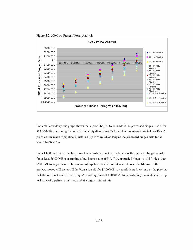
Figure 4.2. 500 Cow Present Worth Analysis

500 Cow PW Analysis

-$1,000,000-$900,000-$800,000-$700,000-$600,000-$500,000-$400,000-$300,000-$200,000-$100,000

$0$100,000$200,000$300,000

$2.00/Mbtu $4.00/Mbtu $6.00/Mbtu $8.00/Mbtu $10.00/Mbtu $12.00/MBtu $14.00/MBtu

Processed Biogas Selling Value ($/MBtu)

PW o

f Pro

cess

ed B

ioga

s Sa

les

3%, No Pipeline

5%, No Pipeline

7%, No Pipeline

3%, 1/4 MilePipeline5%, 1/4 MilePipeline7%, 1/4 MilePipeline3%, 1/2 MilePipeline5%, 1/2 MilePipeline7%, 1/2 MilePipeline3%, 1 Mile Pipeline

5%, 1 Mile Pipeline

7%, 1 Mile Pipeline

For a 500 cow dairy, the graph shows that a profit begins to be made if the processed biogas is sold for

$12.00/MBtu, assuming that no additional pipeline is installed and that the interest rate is low (3%). A

profit can be made if pipeline is installed (up to ½ mile), as long as the processed biogas sells for at

least $14.00/MBtu.

For a 1,000 cow dairy, the data show that a profit will not be made unless the upgraded biogas is sold

for at least $6.00/MBtu, assuming a low interest rate of 3%. If the upgraded biogas is sold for less than

$6.00/MBtu, regardless of the amount of pipeline installed or interest rate over the lifetime of the

project, money will be lost. If the biogas is sold for $8.00/MBtu, a profit is made as long as the pipeline

installation is not over ½ mile long. At a selling price of $10.00/MBtu, a profit may be made even if up

to 1 mile of pipeline is installed and at a higher interest rate.

4-38

Figure 4.3. 1,000 Cow Present Worth Analysis

1,000 Cow PW Analysis

-$1,000,000

-$800,000

-$600,000

-$400,000

-$200,000

$0

$200,000

$400,000

$600,000

$800,000

$1,000,000

$1,200,000

$2.00/Mbtu $4.00/Mbtu $6.00/Mbtu $8.00/Mbtu $10.00/Mbtu $12.00/MBtu $14.00/MBtu

Processed Biogas Selling Value ($/MBtu)

PW o

f Pro

cess

ed B

ioga

s Sa

les

3%, No Pipeline5%, No Pipeline7%, No Pipeline3%, 1/4 Mile Pipeline5%, 1/4 Mile Pipeline7%, 1/4 Mile Pipeline3%, 1/2 Mile Pipeline5%, 1/2 Mile Pipeline7%, 1/2 Mile Pipeline3%, 1 Mile Pipeline5%, 1 Mile Pipeline7%, 1 Mile Pipeline

4-39

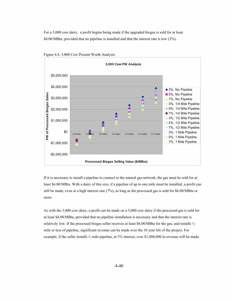
For a 3,000 cow dairy, a profit begins being made if the upgraded biogas is sold for at least

$4.00/MBtu, provided that no pipeline is installed and that the interest rate is low (3%).

Figure 4.4. 3,000 Cow Present Worth Analysis

3,000 Cow PW Analysis

-$2,000,000

-$1,000,000

$0

$1,000,000

$2,000,000

$3,000,000

$4,000,000

$5,000,000

$2.00/Mbtu $4.00/Mbtu $6.00/Mbtu $8.00/Mbtu $10.00/Mbtu $12.00/MBtu $14.00/MBtu

Processed Biogas Selling Value ($/MBtu)

PW o

f Pro

cess

ed B

ioga

s Sa

les

3%, No Pipeline5%, No Pipeline7%, No Pipeline3%, 1/4 Mile Pipeline5%, 1/4 Mile Pipeline7%, 1/4 Mile Pipeline3%, 1/2 Mile Pipeline5%, 1/2 Mile Pipeline7%, 1/2 Mile Pipeline3%, 1 Mile Pipeline5%, 1 Mile Pipeline7%, 1 Mile Pipeline

If it is necessary to install a pipeline to connect to the natural gas network, the gas must be sold for at

least $6.00/MBtu. With a dairy of this size, if a pipeline of up to one mile must be installed, a profit can

still be made, even at a high interest rate (7%), as long as the processed gas is sold for $6.00/MBtu or

more.

As with the 3,000 cow dairy, a profit can be made on a 5,000 cow dairy if the processed gas is sold for

at least $4.00/MBtu, provided that no pipeline installation is necessary and that the interest rate is

relatively low. If the processed biogas seller receives at least $6.00/MBtu for the gas, and installs ½

mile or less of pipeline, significant revenue can be made over the 10 year life of the project. For

example, if the seller installs ½ mile pipeline, at 3% interest, over $1,000,000 in revenue will be made.

4-40

Figure 4.5. 5,000 Cow Present Worth Analysis

5,000 Cow PW Analysis

-$3,000,000

-$2,000,000

-$1,000,000

$0

$1,000,000

$2,000,000

$3,000,000

$4,000,000

$5,000,000

$6,000,000

$7,000,000

$2.00/Mbtu $4.00/Mbtu $6.00/Mbtu $8.00/Mbtu $10.00/Mbtu $12.00/MBtu $14.00/MBtu

Processed Biogas Selling Value ($/MBtu)

PW o

f Pro

cess

ed B

ioga

s Sa

les

3%, No Pipeline5%, No Pipeline7%, No Pipeline3%, 1/4 Mile Pipeline5%, 1/4 Mile Pipeline7%, 1/4 Mile Pipeline3%, 1/2 Mile Pipeline5%, 1/2 Mile Pipeline7%, 1/2 Mile Pipeline3%, 1 Mile Pipeline5%, 1 Mile Pipeline7%, 1 Mile Pipeline

Extrapolating the data, the “break even” price that the processed biogas must sell for on a 10,000 cow

is $3.50/MBtu. If the gas is sold for at least $4.00/MBtu, with no pipeline installation and a low interest

rate (3%), over $1,000,000 in profit can be made over the course of the project. If the gas is sold at a

higher rate ($8.00 – $10.00 per MBtu), a significant profit of approximately $3,832,736 and $5,909,250

can be made, respectively, even if up to one mile of pipeline must be installed and at a high interest rate

(7%).

4-41

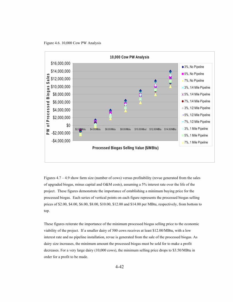
Figure 4.6. 10,000 Cow PW Analysis

10,000 Cow PW Analysis

-$4,000,000

-$2,000,000

$0

$2,000,000

$4,000,000

$6,000,000

$8,000,000

$10,000,000

$12,000,000

$14,000,000

$16,000,000

$2.00/Mbtu $4.00/Mbtu $6.00/Mbtu $8.00/Mbtu $10.00/Mbut $12.00/MBtu $14.00/MBtu

Processed Biogas Selling Value ($/MBtu)

PW o

f Pro

cess

ed B

ioga

s Sa

les

3%, No Pipeline

5%, No Pipeline

7%, No Pipeline

3%, 1/4 Mile Pipeline

5%, 1/4 Mile Pipeline

7%, 1/4 Mile Pipeline

3%, 1/2 Mile Pipeline

5%, 1/2 Mile Pipeline

7%, 1/2 Mile Pipeline

3%, 1 Mile Pipeline

5%, 1 Mile Pipeline

7%, 1 Mile Pipeline

Figures 4.7 – 4.9 show farm size (number of cows) versus profitability (revue generated from the sales

of upgraded biogas, minus capital and O&M costs), assuming a 5% interest rate over the life of the

project. These figures demonstrate the importance of establishing a minimum buying price for the

processed biogas. Each series of vertical points on each figure represents the processed biogas selling

prices of $2.00, $4.00, $6.00, $8.00, $10.00, $12.00 and $14.00 per MBtu, respectively, from bottom to

top.

These figures reiterate the importance of the minimum processed biogas selling price to the economic

viability of the project. If a smaller dairy of 500 cows receives at least $12.00/MBtu, with a low

interest rate and no pipeline installation, revue is generated from the sale of the processed biogas. As

dairy size increases, the minimum amount the processed biogas must be sold for to make a profit

decreases. For a very large dairy (10,000 cows), the minimum selling price drops to $3.50/MBtu in

order for a profit to be made.

4-42

Figure 4.7. Farm Size versus Profitability No Pipeline Installation, 5% Interest

Farm Size Versus Profitability, No Pipeline Installation, 5% Interest

-$2,000,000

$0

$2,000,000

$4,000,000

$6,000,000

$8,000,000

$10,000,000

$12,000,000

$14,000,000

0 1000 2000 3000 4000 5000 6000 7000 8000 9000 10000 11000

Number of Cows on Farm

Pres

ent W

orth

of I

ncom

e

500 Cows

1000 Cows

3,000 Cows

5,000 Cows

10,000 Cows

4-43

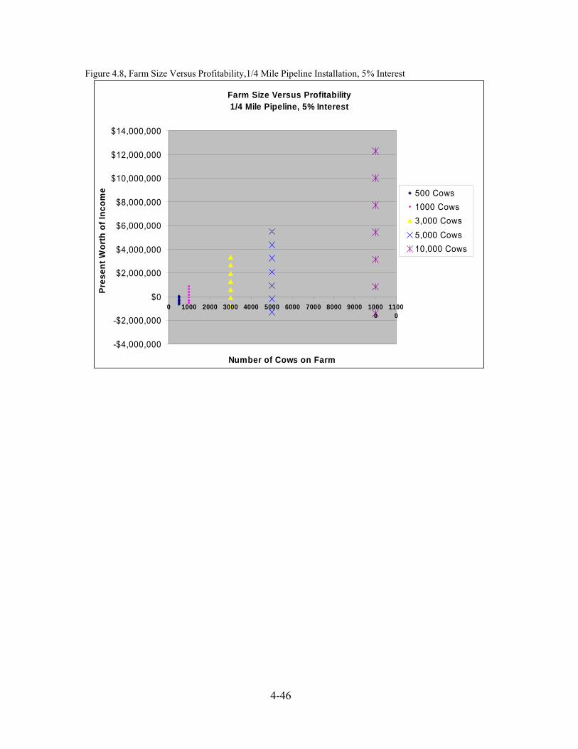
Figure 4.8, Farm Size Versus Profitability,1/4 Mile Pipeline Installation, 5% Interest

Farm Size Versus Profitability1/4 Mile Pipeline, 5% Interest

-$4,000,000

-$2,000,000

$0

$2,000,000

$4,000,000

$6,000,000

$8,000,000

$10,000,000

$12,000,000

$14,000,000

0 1000 2000 3000 4000 5000 6000 7000 8000 9000 10000

11000

Number of Cows on Farm

Pres

ent W

orth

of I

ncom

e 500 Cows1000 Cows3,000 Cows5,000 Cows10,000 Cows

4-46

Figure 4.9. Farm Size Versus Profitability, 1/2 Mile Pipeline Installation, 5% Interest

Farm Size Versus Profitability1/2 Mile Pipeline, 5% Interest

-$4,000,000

-$2,000,000

$0

$2,000,000

$4,000,000

$6,000,000

$8,000,000

$10,000,000

$12,000,000

$14,000,000

0 1000 2000 3000 4000 5000 6000 7000 8000 9000 10000 11000

Number of Cows on Farm

Pres

ent W

orth

of I

ncom

e

500 Cows1,000 Cows3,000 Cows5,000 Cows10,000 Cows

4-47

Figure 4.10. Farm Size Versus Profitability, 1 Mile Pipeline Installation, 5% Interest

Farm Size Versus Profitability1 Mile Pipeline, 5% Interest

-$4,000,000

-$2,000,000

$0

$2,000,000

$4,000,000

$6,000,000

$8,000,000

$10,000,000

$12,000,000

$14,000,000

0 1000 2000 3000 4000 5000 6000 7000 8000 9000 10000

11000

Number of Cows on Farm

Pres

ent W

orth

of I

ncom

e

500 Cows1,000 Cows3,000 Cows5,000 Cows10,000 Cows

4-48

REFERENCES AgSTAR Digest, www.epa.gov/agstar, Spring 2002. AgSTAR Industry Directory for On-Farm Biogas Recovery Systems, www.epa.gov/agstar, Spring 2000. Alderfer, R.B., M.M. Eldridge, and T.J. Starrs, Making Connections: Case Studies of Interconnection Barriers and Their Impact on Distributed Power Projects, Report National Renewable Energy Laboratory: NREL/SR-200-28053, 2000. Anerousis, J.P., and S.K. Whitman, Iron Sponge: Still a Top Option for Sour Gas Sweetening, Oil and Gas Journal, 71-76, 1985. Bentzen,G., A.T. Smith, D. Bennett, N. J. Webster, F. Reinholt, E. Sletholt, and J. Hobson. 1995. Controlled Dosing of Nitrate for Prevention of H2S in a Sewer Network and the Effects of the Subsequent Treatment Processs. Water Science and Technology. 31(7): 293-302. Capstone Low Emissions MicroTurbine Technology: White Paper, Capstone Turbine Corporation, Chatsworth, CA, July 19, 2000. http://www.auxenergy.com/Emissions.pdf Capstone Operations Manual, Capstone Turbine Corporation, Model 330, 2000. Carlsen, H., Bovin, J., Stirling Engines in Small CHP Plants, 2001 Degorce-Dumas, H.R., S. Kowal, and P. LeCloirec, Microbiological Oxidation of Hydrogen Sulphide in a Biofilter, Canadian Journal of Microbiology, Vol. 43, 263-271, 1997. Foral, A.J., and B.H. Al-Ubaidi, Evaluation of H2S Scavenger Technologies, GRI Report No. GRI-94/0197, 1994. Knoblauch, W.A., L.D. Putnam, and J. Karszes, Dairy Management:Business Summary New York State 2000, Department of Applied Economics and Mangement, Cornell University, October 2001. Minott, S.J. and Scott, N.R., Feasibility of Fuel Cells for Energy Conversion on Dairy Farms, ASAE Paper 01-7015, July 2001. Minott, S., Tejasen, K., Ratterman, S., Graf, K., and Kalman-Blustein, R. New York State Potential for Biomass Energy Production from Dairy Farms. Technical Report, Cornell University, 2000. Nicolai, R.E. and K.A. Janni, Development of a Low-Cost Biofilter for Swine Production Facilities, ASAE Paper No. 97-4040, 1997. NYSERDA Project 6243, Feasibility of Fuel Cells for Energy Conversion on the Dairy Farm, 2000. NYSERDA Project 6597, Biogas Distributed Generation Systems Evaluation and Technology Transfer, 2001. Pellerin, R.A., L.P. Walker, M.G. Heisler, and G.S. Farmer, Operation and Performance of Biogas-Fueled Cogeneration Systems, Energy in Agriculture, Vol. 6, 295-310, 1987. Prabhu, E., The Flex-Microturbine Uniquely Adapted to Low-Pressure Biomass Gasses, CEC Contract No. 500-99-030, November, 2001. Revel, C., Personal Correspondence, Connelly-GPM, Inc., March 2001.

5-1

Schomaker, A., A. Boerboom, A. Visser, and A. Pfeifer, Anaerobic Digestion of Agro-Industrial Wastes: Information Networks: Technical Summary on Gas Treatment, AD-NETT Project FAIR-CT96-2083 (DG12-SSMI), January, 2000. Scott, N.R., NYSERDA Innovations in Agriculture Workshop PowerPoint Presentation, November, 2001. The SulfaTreat Company, www.SulfaTreat.com, Chesterfield, Missouri, USA 63005. Yang, Y., and E.R.Allen, Biofiltration Control of Hydrogen Sulfide. 1. Design and Operational Parameters, Journal of Air and Waste Management Association, Vol. 44, 863-868, July 1994. Zhang, R.H, P.N. Dugba, and D.S. Bundy, Laboratory Study of Surface Aeration of Anaerobic lagoons for Odor Control of Swine Manure, Transactions of the ASAE, Vol. 40(1), 185-190, 1997. Zicari, S., Removal of Hydrogen Sulfide from Biogas Using Cow-Manure Compost , MS Thesis, Cornell University, January 2003.

5-2

APPENDIX A

Tedlar Bag - Sample Integrity Study Using Hydrogen SulfideSeptember 7-8, 2003

0

1000

2000

3000

4000

5000

6000

7000

8000

0 5 10 15 20 25 30

Sample Storage Time (hours)

H2S

Con

cent

ratio

n (p

pm) Sample 1000A

Sample 1000BSample 1000CSample 2500ASample 2500BSample 2500CSample 5000ASample 5000BSample 5000C

Figure A-1 Test of the rate of decline in hydrogen sulfide from Tedlar sampling bags.

A-1

APPENDIX B

Gas Composition Curves

B-1

Average H2S in Raw Biogas at AA Dairy

0

500

1000

1500

2000

2500

3000

3500

4000

4500

6/28/0

3

8/17/0

3

10/06

/03

11/25

/03

1/14/0

4

3/04/0

4

4/23/0

4

Date

Figure B-1 Average H2S measured in biogas at AA Dairy, July 2003- March 2004

58

58.5

59

59.5

60

60.5

61

61.5

62

Time

% M

etha

ne

25-Jul-0326-Jul-0327-Jul-0328-Jul-0329-Jul-0330-Jul-0331-Jul-03

Figure B-2 Daily Average Methane Concentration in Biogas at DDI (July 2003)

B-2

58

58.5

59

59.5

60

60.5

61

61.5

62

00:00

:00

02:24

:00

04:48

:00

07:12

:00

09:36

:00

12:00

:00

14:24

:00

16:48

:00

19:12

:00

21:36

:00

00:00

:00

Time

% M

etha

ne

21-Aug-03

22-Aug-03

23-Aug-03

24-Aug-03

25-Aug-03

26-Aug-03

27-Aug-03

Figure B-3 Daily Average Methane Concentration in Biogas at DDI (August 2003)

58

58.5

59

59.5

60

60.5

61

61.5

62

Time

% M

etha

ne

03-Sep-0304-Sep-0305-Sep-0306-Sep-0307-Sep-0308-Sep-0309-Sep-03

Figure B-4 Daily Average of Methane Concentration in Biogas at DDI (September 2003)

B-3

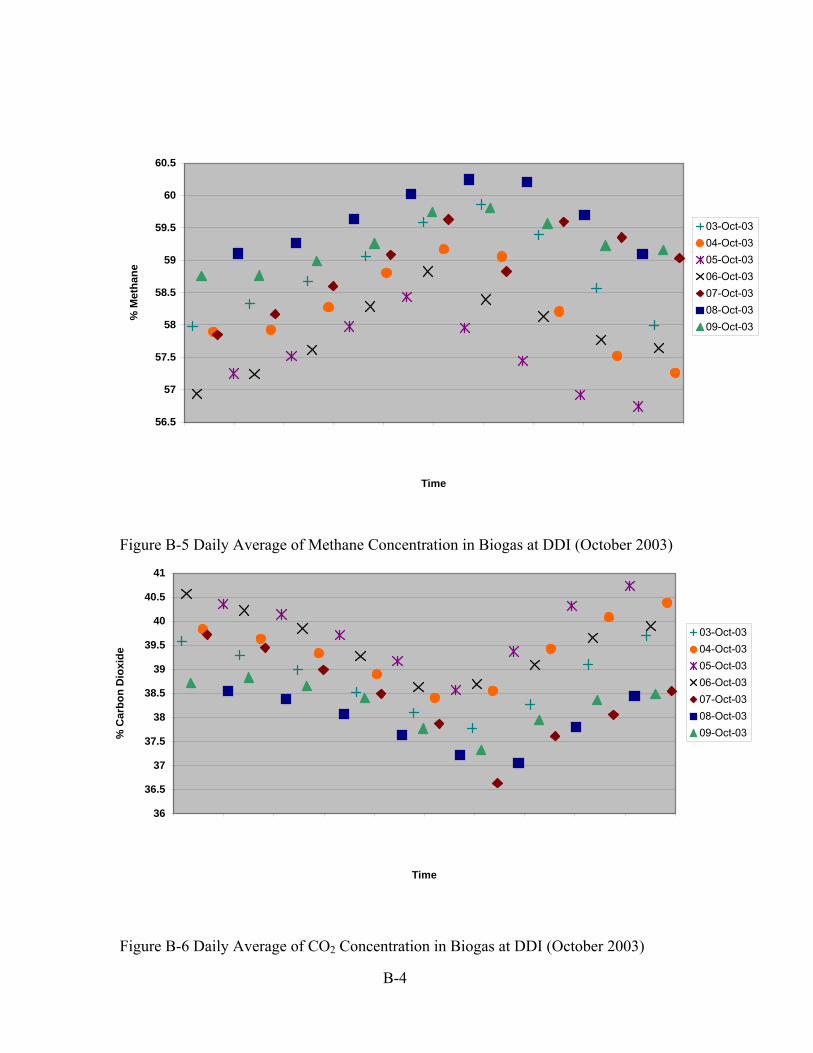
56.5

57

57.5

58

58.5

59

59.5

60

60.5

Time

% M

etha

ne

03-Oct-0304-Oct-0305-Oct-0306-Oct-0307-Oct-0308-Oct-0309-Oct-03

Figure B-5 Daily Average of Methane Concentration in Biogas at DDI (October 2003)

36

36.5

37

37.5

38

38.5

39

39.5

40

40.5

41

Time

% C

arbo

n D

ioxi

de

03-Oct-0304-Oct-0305-Oct-0306-Oct-0307-Oct-0308-Oct-0309-Oct-03

Concentration in Biogas at DDI (October 2003) Figure B-6 Daily Average of CO2

B-4

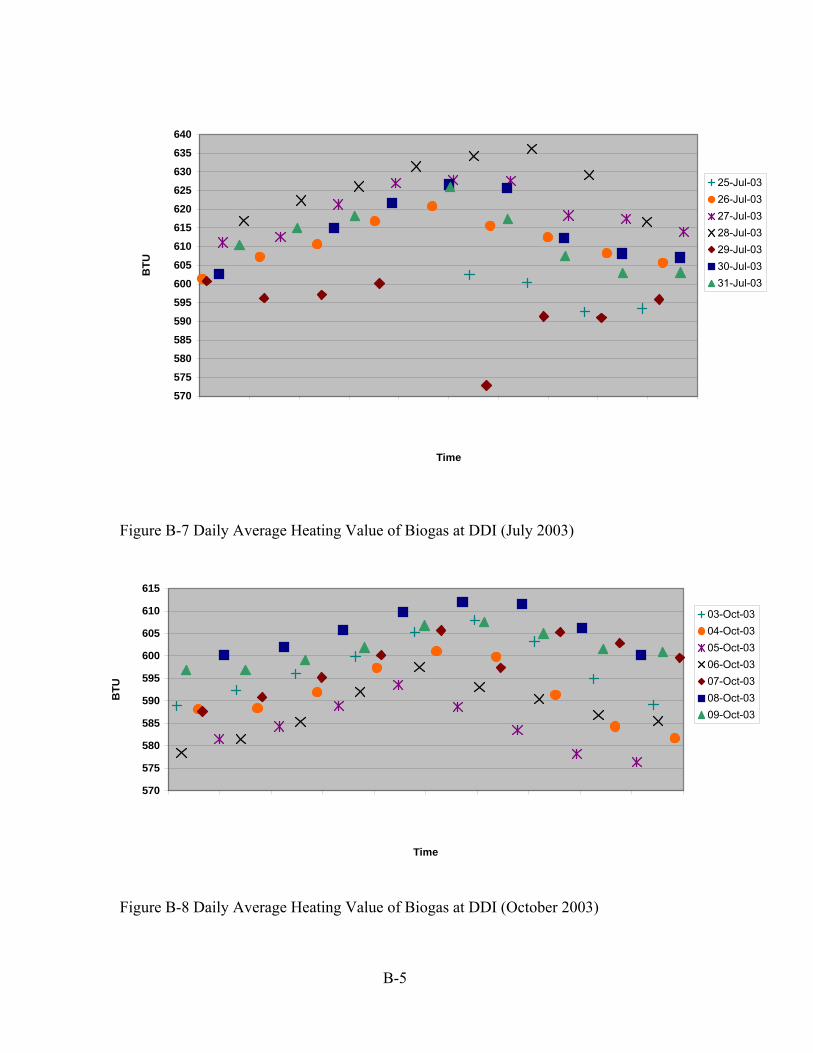
570

575

580

585

590

595

600

605

610

615

620

625

630

635

640

Time

BTU

25-Jul-0326-Jul-0327-Jul-0328-Jul-0329-Jul-0330-Jul-0331-Jul-03

Figure B-7 Daily Average Heating Value of Biogas at DDI (July 2003)

570

575

580

585

590

595

600

605

610

615

Time

BTU

03-Oct-0304-Oct-0305-Oct-0306-Oct-0307-Oct-0308-Oct-0309-Oct-03

Figure B-8 Daily Average Heating Value of Biogas at DDI (October 2003)

B-5

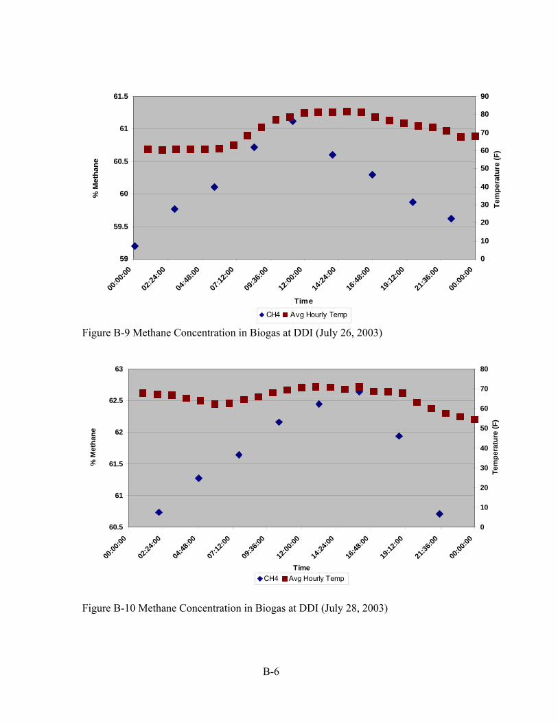
59

59.5

60

60.5

61

61.5

00:00

:00

02:24

:00

04:48

:00

07:12

:00

09:36

:00

12:00

:00

14:24

:00

16:48

:00

19:12

:00

21:36

:00

00:00

:00

Time

% M

etha

ne

0

10

20

30

40

50

60

70

80

90

Tem

pera

ture

(F)

CH4 Avg Hourly Temp

Figure B-9 Methane Concentration in Biogas at DDI (July 26, 2003)

60.5

61

61.5

62

62.5

63

00:00

:00

02:24

:00

04:48

:00

07:12

:00

09:36

:00

12:00

:00

14:24

:00

16:48

:00

19:12

:00

21:36

:00

00:00

:00

Time

% M

etha

ne

0

10

20

30

40

50

60

70

80

Tem

pera

ture

(F)

CH4 Avg Hourly Temp

Figure B-10 Methane Concentration in Biogas at DDI (July 28, 2003)

B-6

58.8

59

59.2

59.4

59.6

59.8

60

60.2

60.4

60.6

60.8

00:00

:00

02:24

:00

04:48

:00

07:12

:00

09:36

:00

12:00

:00

14:24

:00

16:48

:00

19:12

:00

21:36

:00

00:00

:00

Time

% M

etha

ne

0

10

20

30

40

50

60

70

80

Tem

pera

ture

(F)

CH4 Avg Hourly Temp

Figure B-11 Methane Concentration in Biogas at DDI (August 23, 2003)

59.5

60

60.5

61

61.5

62

00:00

:00

02:24

:00

04:48

:00

07:12

:00

09:36

:00

12:00

:00

14:24

:00

16:48

:00

19:12

:00

21:36

:00

00:00

:00

Time

% M

etha

ne

0

10

20

30

40

50

60

70

80

Tem

pera

ture

(F)

CH4 Avg Hourly Temp

Figure B-12 Methane Concentration in Biogas at DDI (August 24, 2003)

B-7

57

57.5

58

58.5

59

59.5

00:00

:00

02:24

:00

04:48

:00

07:12

:00

09:36

:00

12:00

:00

14:24

:00

16:48

:00

19:12

:00

21:36

:00

00:00

:00

Time

% M

etha

ne

0

10

20

30

40

50

60

70

80

Tem

pera

ture

(F)

CH4 Avg Hourly Temp

Figure B-13 Methane Concentration in Biogas at DDI (September 4, 2003)

56.6

56.8

57

57.2

57.4

57.6

57.8

58

58.2

58.4

58.6

00:00

:00

02:24

:00

04:48

:00

07:12

:00

09:36

:00

12:00

:00

14:24

:00

16:48

:00

19:12

:00

21:36

:00

00:00

:00

Time

% M

etha

ne

0

10

20

30

40

50

60

70

Tem

pera

ture

(F)

CH4 Avg Hourly Temp

Figure B-14 Methane Concentration in Biogas at DDI (September 5, 2003)

B-8

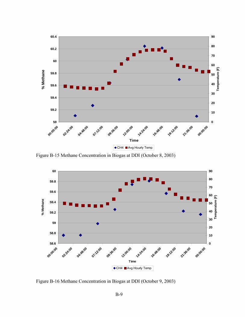
59

59.2

59.4

59.6

59.8

60

60.2

60.4

00:00

:00

02:24

:00

04:48

:00

07:12

:00

09:36

:00

12:00

:00

14:24

:00

16:48

:00

19:12

:00

21:36

:00

00:00

:00

Time

% M

etha

ne

0

10

20

30

40

50

60

70

80

90

Tem

pera

ture

(F)

CH4 Avg Hourly Temp

Figure B-15 Methane Concentration in Biogas at DDI (October 8, 2003)

58.6

58.8

59

59.2

59.4

59.6

59.8

60

00:00

:00

02:24

:00

04:48

:00

07:12

:00

09:36

:00

12:00

:00

14:24

:00

16:48

:00

19:12

:00

21:36

:00

00:00

:00

Time

% M

etha

ne

0

10

20

30

40

50

60

70

80

90

Tem

pera

ture

(F)

CH4 Avg Hourly Temp

Figure B-16 Methane Concentration in Biogas at DDI (October 9, 2003)

B-9