Embed Size (px)
Citation preview
Biometrical Genetics
Lindon Eaves,VIPBG Richmond
Boulder CO, 2012
Biometrical Genetics
How do genes contribute to statistics (e.g. means, variances,skewness,
kurtosis)?
Some Literature:
Jinks JL, Fulker DW (1970): Comparison of the biometrical genetical, MAVA, and classical approaches to the analysis of human behavior. Psychol Bull 73(5):311‐349.
Kearsy MJ, Pooni HS (1996) The Genetic Analysis of Quantitative Traits. London UK: Chapman Hall.
Falconer DS, Mackay TFC (1996). Introduction to Quantitative Genetics, 4th Ed. Harlow, UK: Addison Wesley Longman.
Neale MC, Cardon LR (1992). Methodology for Genetic Studies of Twins and Families. Ch 3. Dordrecht: Kluwer Academic Publisher. (See revised ed. Neale and Maes, pdf on VIPBG website)
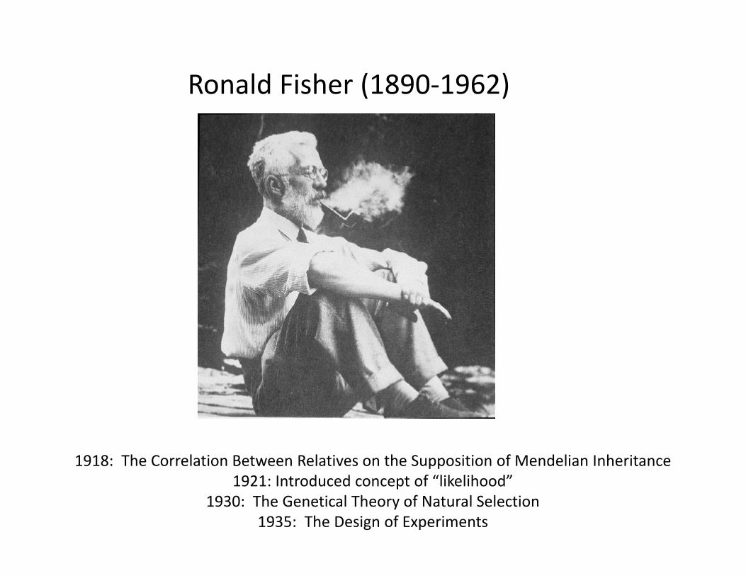
Ronald Fisher (1890‐1962)
1918: The Correlation Between Relatives on the Supposition of Mendelian Inheritance1921: Introduced concept of “likelihood”
1930: The Genetical Theory of Natural Selection1935: The Design of Experiments
Fisher (1918): Basic Ideas
• Continuous variation caused by lots of genes (“polygenic inheritance”)
• Each gene followed Mendel’s laws• Environment smoothed out genetic differences• Genes may show different degrees of “dominance”• Genes may have many forms (“mutliple alleles”)• Mating may not be random (“assortative mating”)• Showed that correlations obtained by e.g. Pearson and Lee were explained well by polygenic inheritance
0 1 2 3 4 5Y1
0.0
0.1
0.2
0.3
0.4
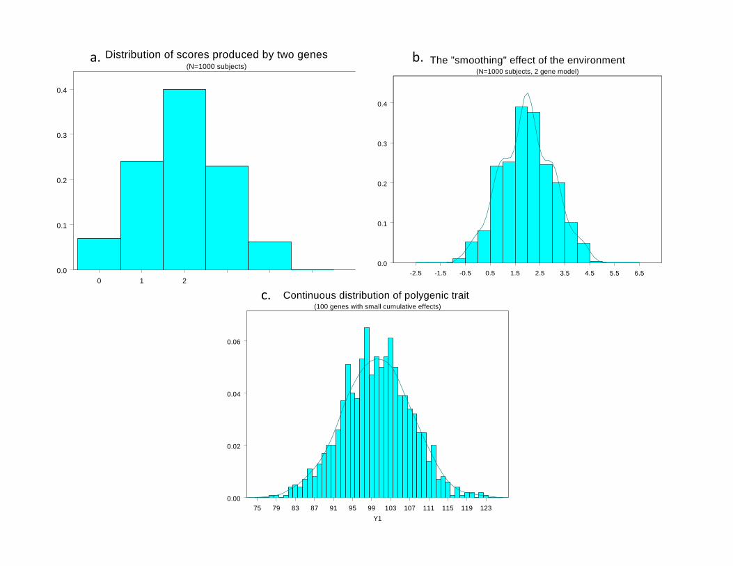
Distribution of scores produced by two genes(N=1000 subjects)
-2.5 -1.5 -0.5 0.5 1.5 2.5 3.5 4.5 5.5 6.5S1
0.0
0.1
0.2
0.3
0.4
The "smoothing" effect of the environment(N=1000 subjects, 2 gene model)
75 79 83 87 91 95 99 103 107 111 115 119 123Y1
0.00
0.02
0.04
0.06
Continuous distribution of polygenic trait (100 genes with small cumulative effects)
b.
c.
a.
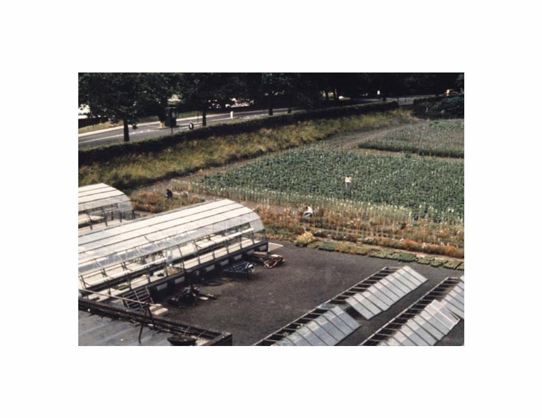
“Mendelian” Crosseswith Quantitative Traits
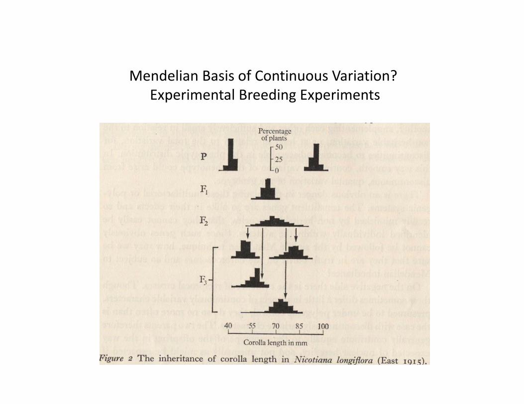
Mendelian Basis of Continuous Variation?Experimental Breeding Experiments
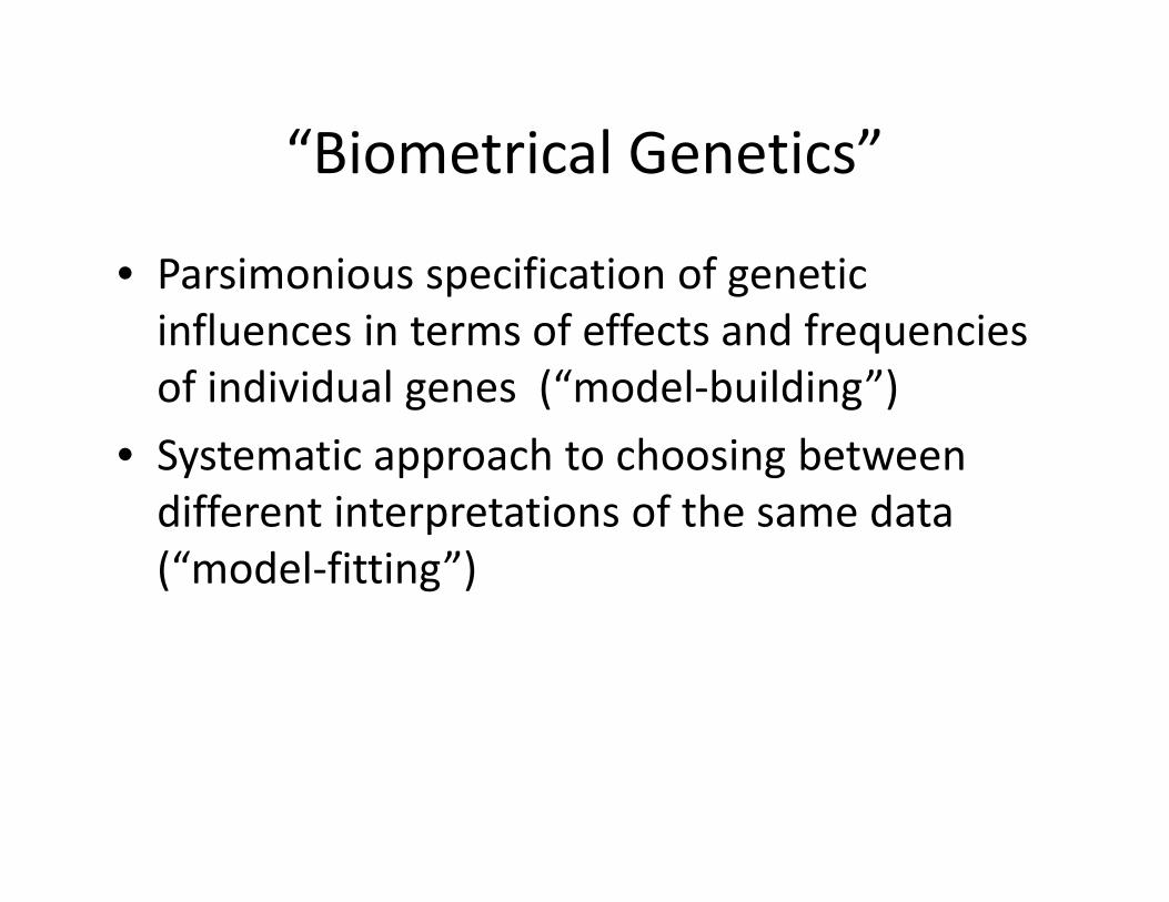
“Biometrical Genetics”
• Parsimonious specification of genetic influences in terms of effects and frequencies of individual genes (“model‐building”)
• Systematic approach to choosing between different interpretations of the same data (“model‐fitting”)
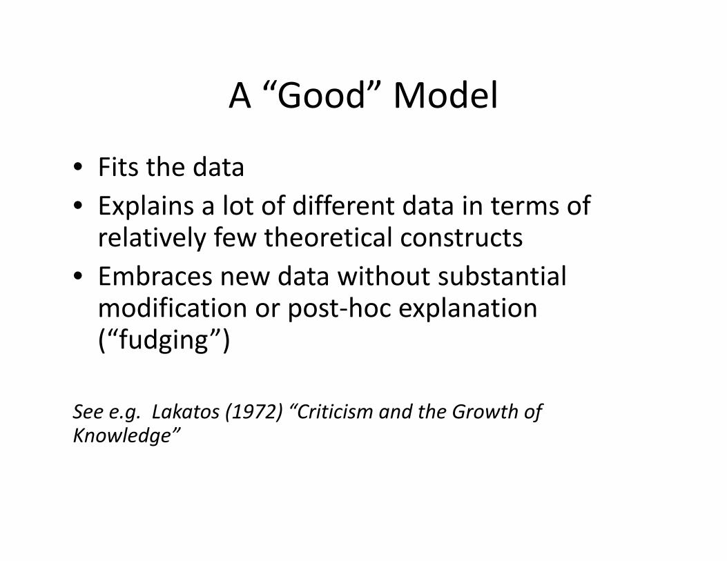
A “Good” Model
• Fits the data• Explains a lot of different data in terms of relatively few theoretical constructs
• Embraces new data without substantial modification or post‐hoc explanation (“fudging”)
See e.g. Lakatos (1972) “Criticism and the Growth of Knowledge”
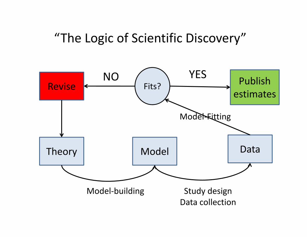
Theory Model Data
Model‐building Study designData collection
Model‐Fitting
Fits?Revise Publishestimates
YESNO
“The Logic of Scientific Discovery”
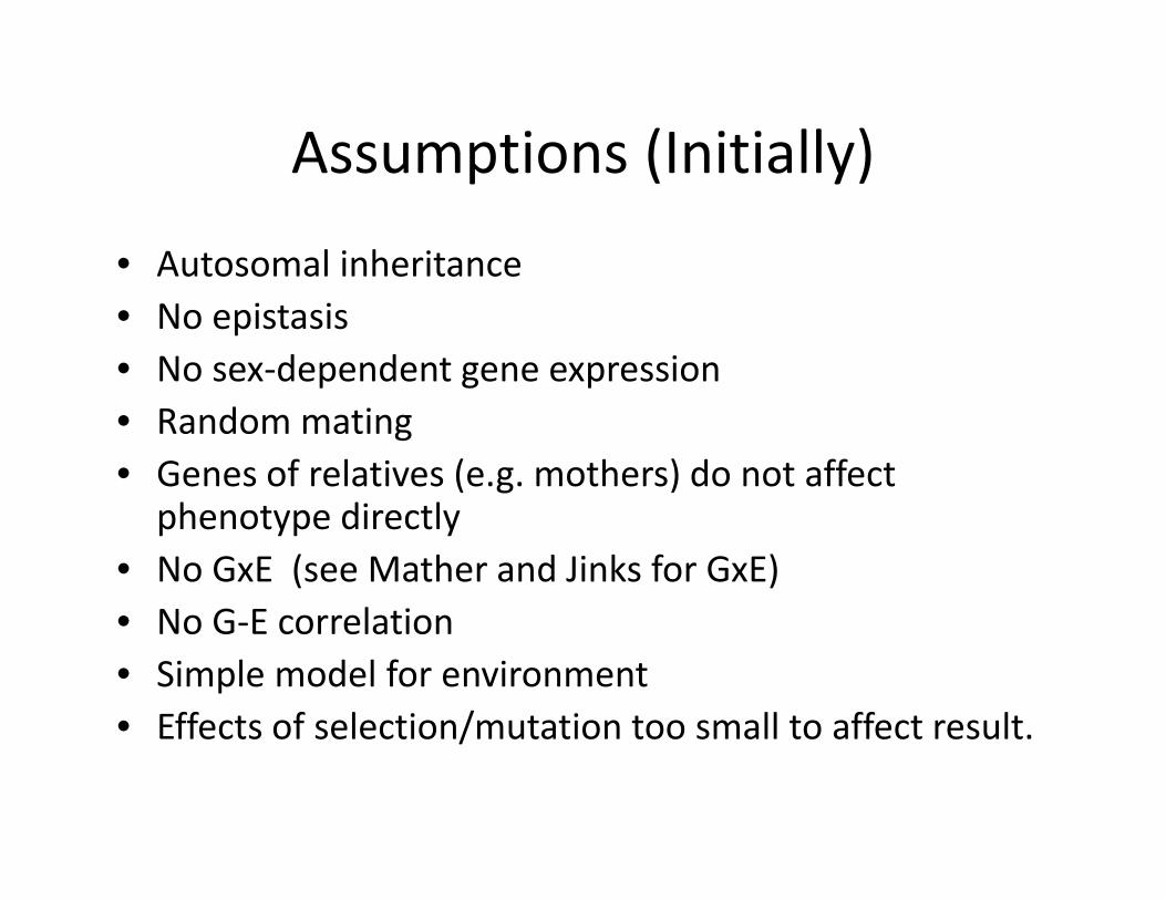
Assumptions (Initially)
• Autosomal inheritance• No epistasis• No sex‐dependent gene expression• Random mating• Genes of relatives (e.g. mothers) do not affect phenotype directly
• No GxE (see Mather and Jinks for GxE)• No G‐E correlation• Simple model for environment• Effects of selection/mutation too small to affect result.
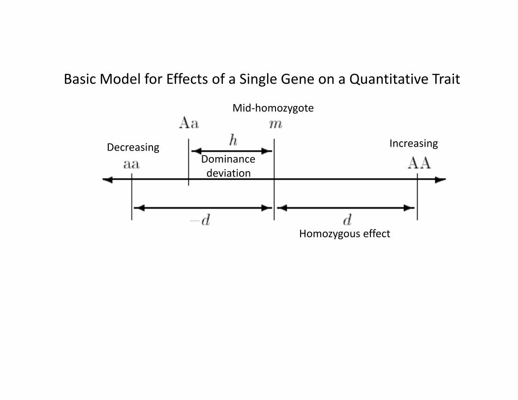
Basic Model for Effects of a Single Gene on a Quantitative Trait
Mid‐homozygote
Homozygous effect
Dominancedeviation
Increasing Decreasing
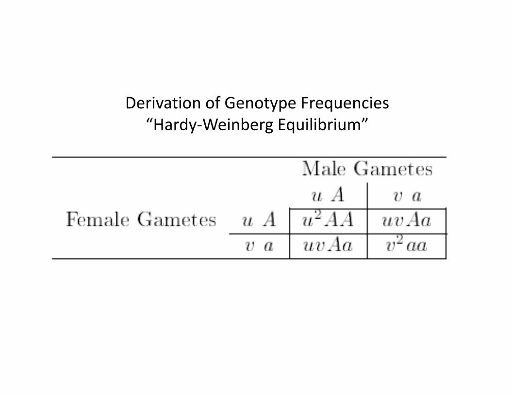
Derivation of Genotype Frequencies“Hardy‐Weinberg Equilibrium”
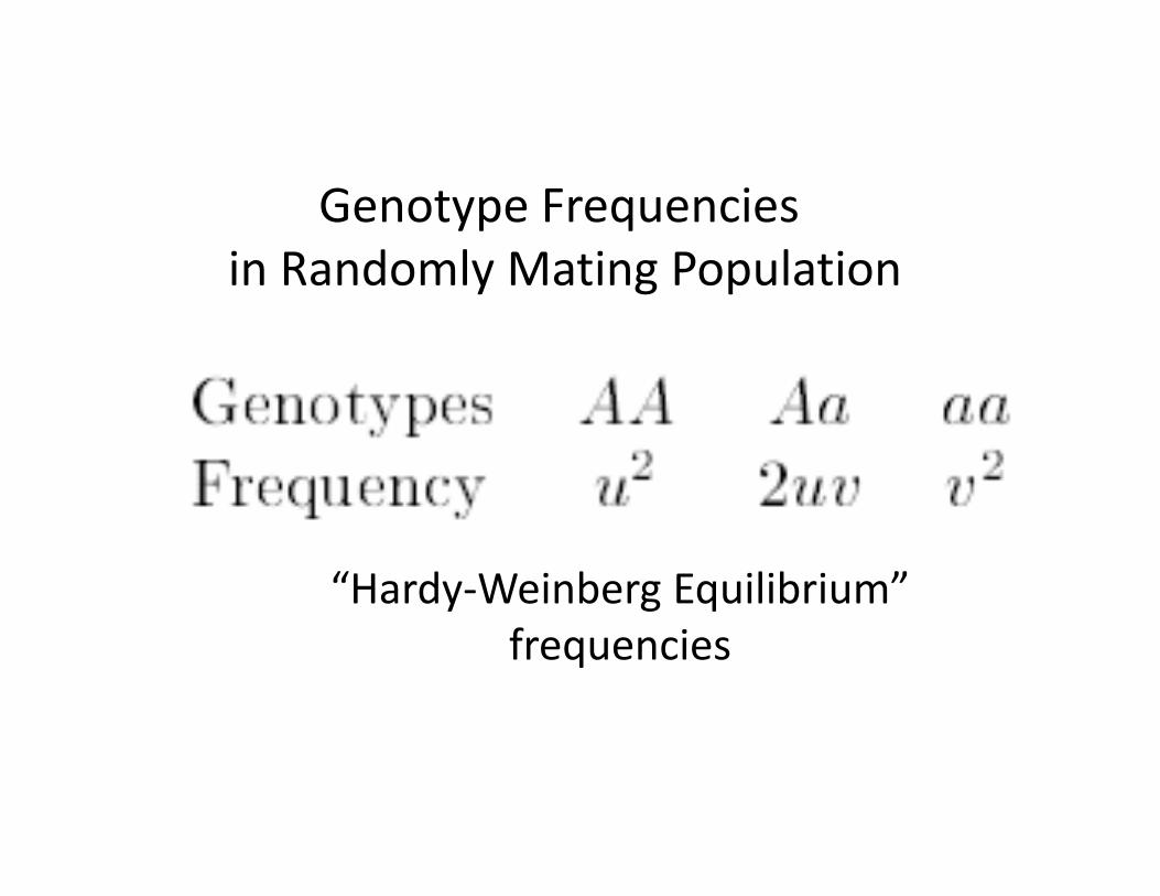
Genotype Frequenciesin Randomly Mating Population
“Hardy‐Weinberg Equilibrium”frequencies
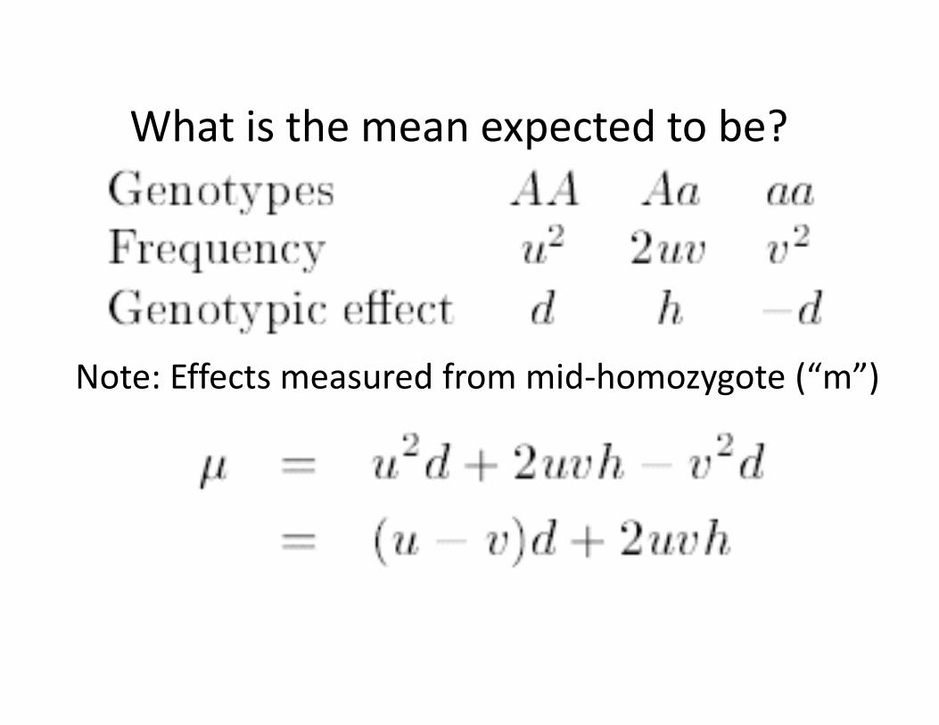
What is the mean expected to be?
Note: Effects measured from mid‐homozygote (“m”)
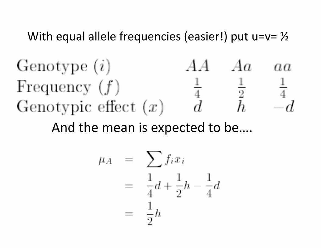
With equal allele frequencies (easier!) put u=v= ½
And the mean is expected to be….
How does A/a affect the variance?
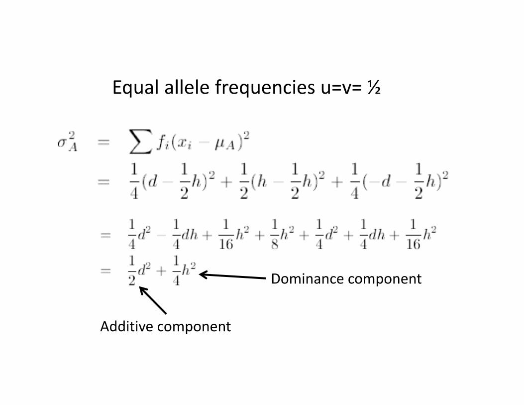
Equal allele frequencies u=v= ½
Additive component
Dominance component
Q: What happens with lots of genes?
A: The effects of the individual genes add up.
IF… the genes are independent (“linkage equilibrium”)
Requires random mating, complete admixture
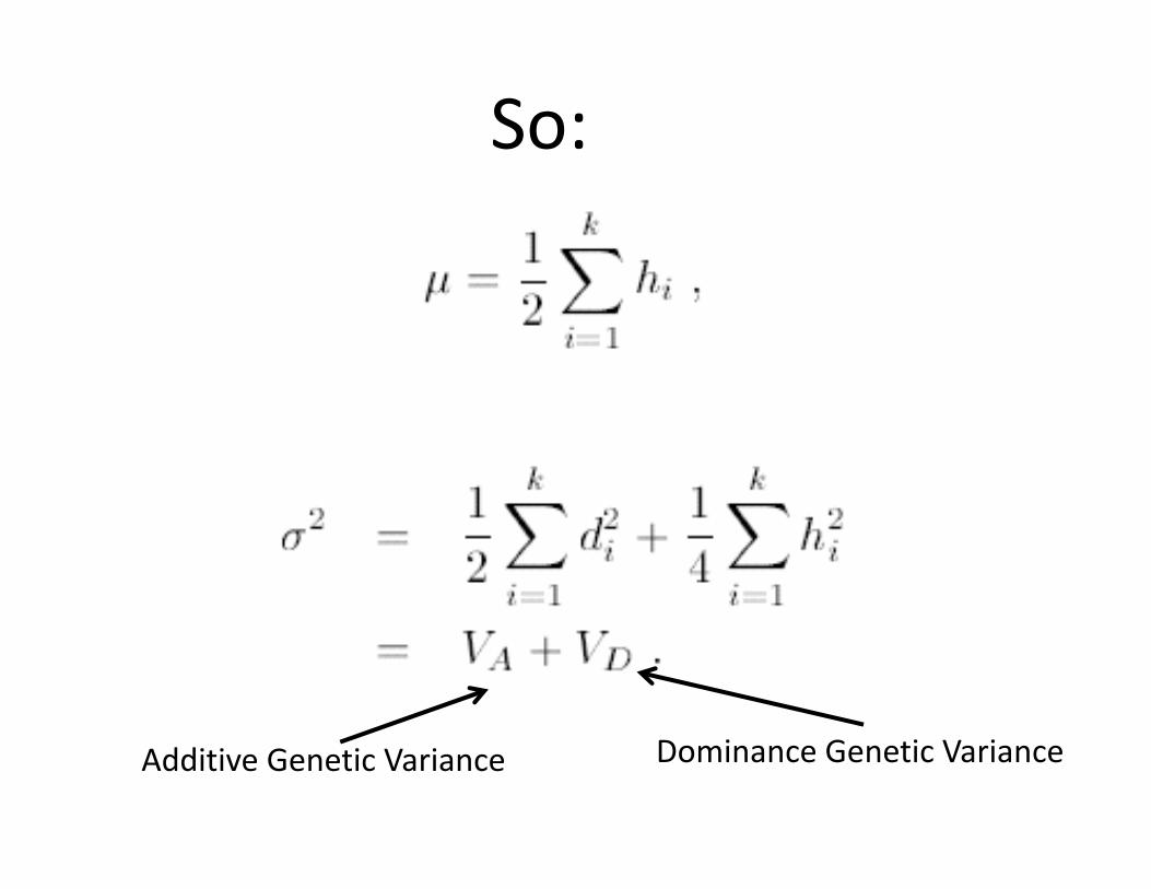
So:
Additive Genetic Variance Dominance Genetic Variance
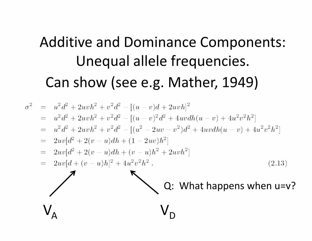
Additive and Dominance Components:Unequal allele frequencies.
Can show (see e.g. Mather, 1949)
VA VD
Q: What happens when u=v?
Bottom line:
With unequal allele frequencies can still separate VA and VD but their
definitions change
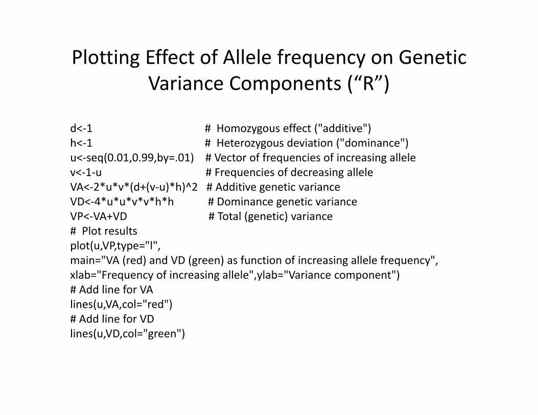
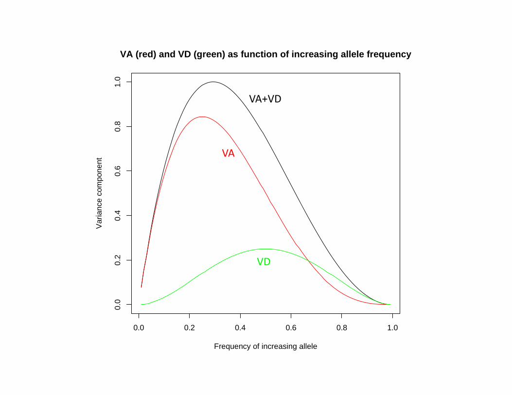
d<‐1 # Homozygous effect ("additive")h<‐1 # Heterozygous deviation ("dominance")u<‐seq(0.01,0.99,by=.01) # Vector of frequencies of increasing allelev<‐1‐u # Frequencies of decreasing alleleVA<‐2*u*v*(d+(v‐u)*h)^2 # Additive genetic varianceVD<‐4*u*u*v*v*h*h # Dominance genetic varianceVP<‐VA+VD # Total (genetic) variance# Plot resultsplot(u,VP,type="l",main="VA (red) and VD (green) as function of increasing allele frequency",xlab="Frequency of increasing allele",ylab="Variance component")# Add line for VAlines(u,VA,col="red")# Add line for VDlines(u,VD,col="green")
Plotting Effect of Allele frequency on Genetic Variance Components (“R”)
0.0 0.2 0.4 0.6 0.8 1.0
0.0
0.2
0.4
0.6
0.8
1.0
VA (red) and VD (green) as function of increasing allele frequency
Frequency of increasing allele
Var
ianc
e co
mpo
nent
VA+VD
VA
VD

What about the environment???
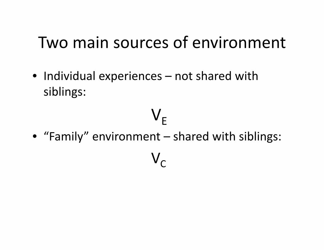
Two main sources of environment
• Individual experiences – not shared with siblings:
VE• “Family” environment – shared with siblings:
VC
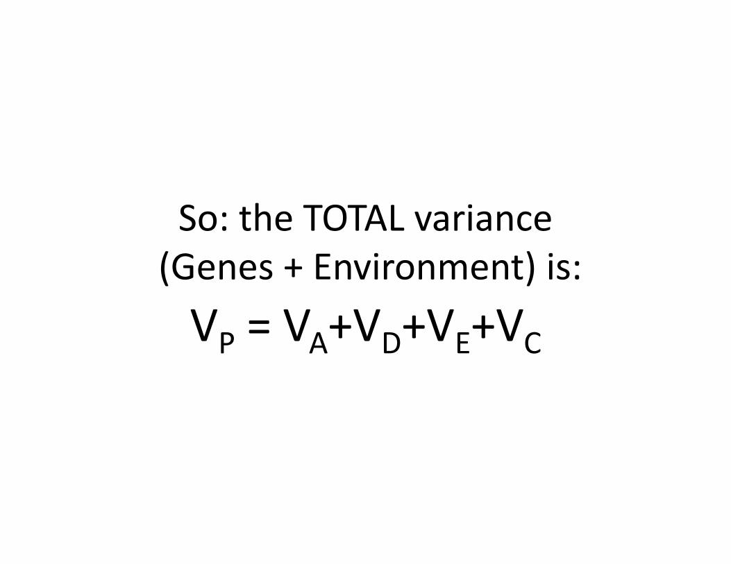
So: the TOTAL variance(Genes + Environment) is:VP = VA+VD+VE+VC
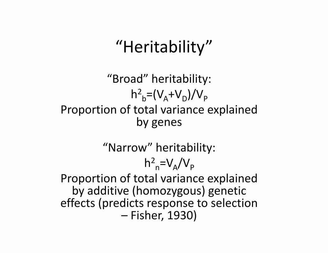
“Heritability”
“Broad” heritability: h2b=(VA+VD)/VP
Proportion of total variance explained by genes
“Narrow” heritability: h2n=VA/VP
Proportion of total variance explained by additive (homozygous) genetic
effects (predicts response to selection – Fisher, 1930)
So far: have looked at effects on total variance…
How do VA and VD affect the correlations between relatives?
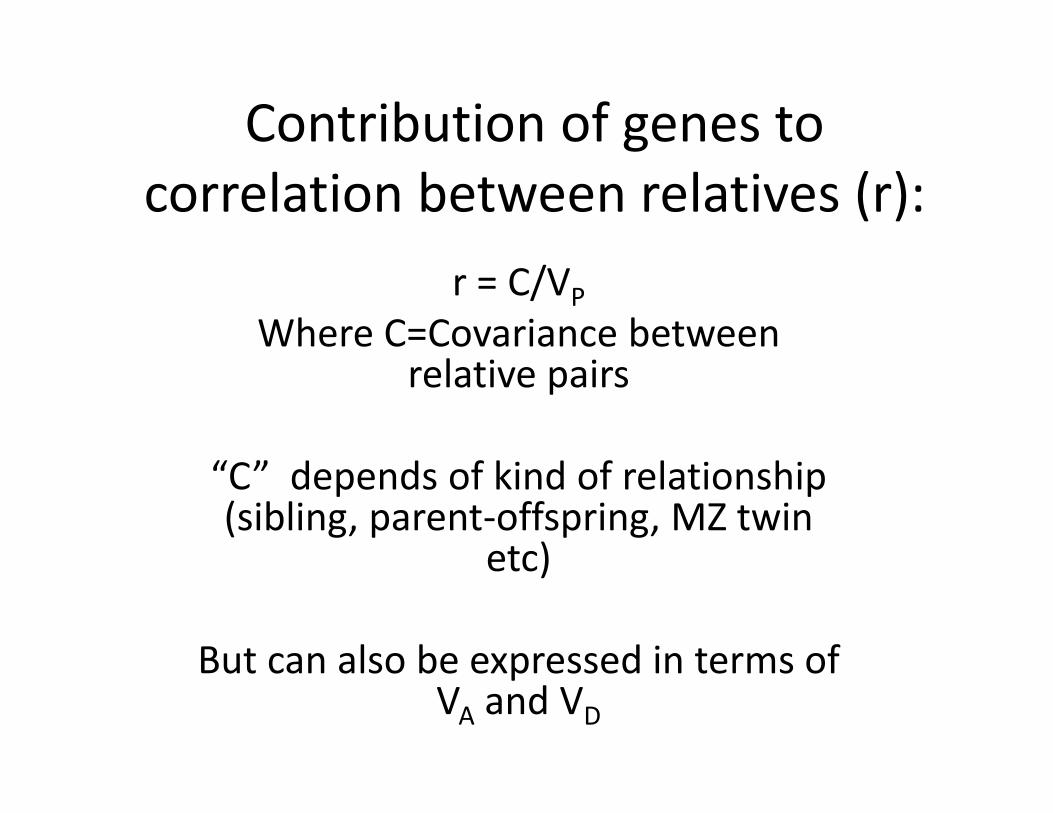
Contribution of genes to correlation between relatives (r):
r = C/VPWhere C=Covariance between
relative pairs
“C” depends of kind of relationship (sibling, parent‐offspring, MZ twin
etc)
But can also be expressed in terms of VA and VD
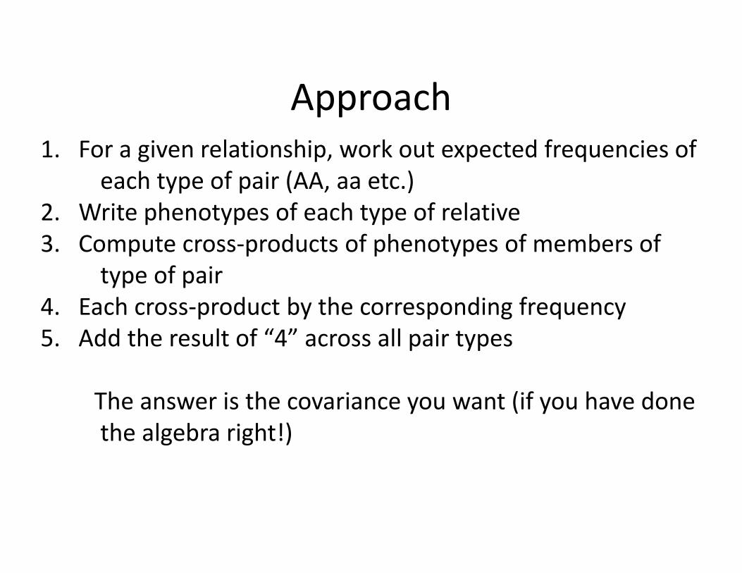
Approach1. For a given relationship, work out expected frequencies of
each type of pair (AA, aa etc.)2. Write phenotypes of each type of relative3. Compute cross‐products of phenotypes of members of
type of pair4. Each cross‐product by the corresponding frequency5. Add the result of “4” across all pair types
The answer is the covariance you want (if you have donethe algebra right!)
For equal allele frequencies….
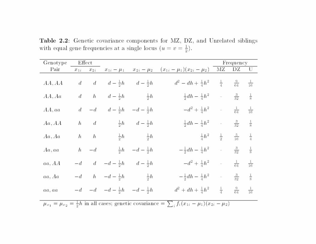
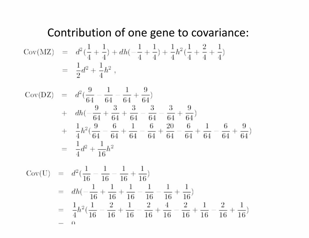
Contribution of one gene to covariance:
Notice that terms in d2 and h2 are separated – but their coefficients
change as a function of relationship
Can add over all genes to get total contribution to covariance
Cov(MZ) = VA + VDCov(DZ) = ½VA + ¼VD
Cov(U)= 0
Can use the same approach for other relationships
RelationshipContribution to Covariance
VA VD
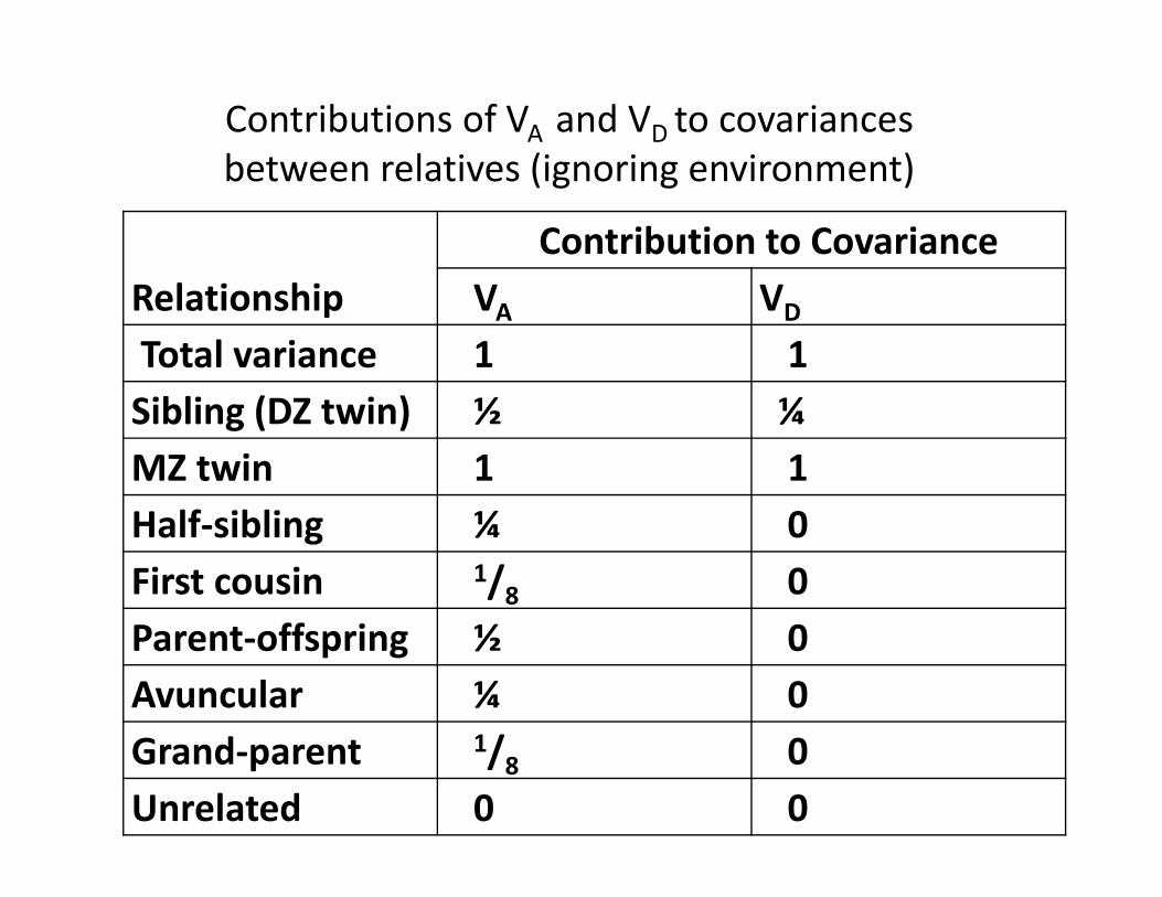
Total variance 1 1Sibling (DZ twin) ½ ¼ MZ twin 1 1Half‐sibling ¼ 0First cousin 1/8 0Parent‐offspring ½ 0Avuncular ¼ 0Grand‐parent 1/8 0Unrelated 0 0
Contributions of VA and VD to covariancesbetween relatives (ignoring environment)
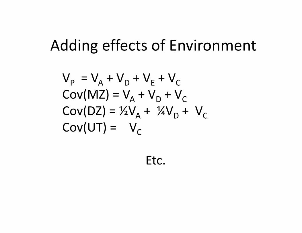
Adding effects of Environment
VP = VA + VD + VE + VCCov(MZ) = VA + VD + VCCov(DZ) = ½VA + ¼VD + VCCov(UT) = VC
Etc.
To get the expected correlations
Just divided expectations by expected total variance
Results are proportional contributions of VA, VD etc. to total variance
Practice (paper and pencil)
• Pick a “d” and “h” (e.g. d=1,h=1; d=1,h=0)• Pick a frequency for the increasing (A) allele (e.g. u=0.2, u=0.7)
• Work out VA and VD• Tabulate on board