Biomolecular modeling I - KITcbp.cfn.kit.edu/downloads/CB-praktikum-WS2015/CB-praktikum-2015-1.pdf · Simulation { we need a model to describe the interactions of atoms { the quality

Molecular mechanicsMolecular dynamics simulation

Introducing thermodynamics

Biomolecular modeling I

Marcus Elstner and Tomas Kubar

2015, December 15

Marcus Elstner and Tomas Kubar Biomolecular modeling I



Biomolecular simulation

Elementary body – atomEach atom – x , y , z coordinates“A protein is a set of coordinates.” (Gromacs, A. P. Heiner)

Usually – one molecule/complex of interest (e.g. protein, NA)




Biomolecular simulation

Elementary body – atomEach atom – x , y , z coordinates“A protein is a set of coordinates.” (Gromacs, A. P. Heiner)

Usually – one molecule/complex of interest (e.g. protein, NA)

Simulation vs. realityOne molecule instead of manyTiny volume of ≈ 10−21 L instead of ≈ 10−5 LSimulation of dynamics – short time scale of max. ≈ 10−5 s




Simulation vs. reality

Why should we want to simulate molecular systems?

Experiment – the molecule has its genuine propertiesSimulation – we need a model to describe the interactions of atoms

– the quality of the model is decisive

Advantage of simulation – structure on atomic level defined

Structure → function

Combination of experiment and simulation – added value
























Molecular mechanics

classical description of molecules




Motivation

To investigate the function of biomolecules,we need to characterize its structure and dynamics.

We will look how the molecules are moving– Molecular Dynamics

For this, we need to calculate the forces on atomsand the energy of the system

Energy from quantum mechanics / quantum chemistry

seemingly easy E =⟨

Ψ∣∣∣H∣∣∣Ψ⟩

but not quite possible for large molecular systems




Motivation






Ψ∣∣∣H∣∣∣Ψ⟩





Motivation






Ψ∣∣∣H∣∣∣Ψ⟩





Motivation






Ψ∣∣∣H∣∣∣Ψ⟩





Motivation




Idea of molecular mechanics

often – well localized bonding orbitals (organic molecules)

idea – similar bonds have similar strength and propertiese.g. similar C–H σ-orbitals → all C–H bonds are ‘similar’

possibly by a harmonic spring? (the simplest possible function)

E (x) =1

2k(x − x0)2

F (x) = −∂E (x)

∂x= −k(x − x0)

2 parameters k and x0 with defined meaning– can be obtained from spectroscopy




Concept of (atom, bond. . . ) type

let us use harmonic springs for covalent bonds

we do not want to parametrize k and x0 each bond separately

use just several sets (k , x0), for different types of bonds

Why can we expect such ‘unification’ to work?





Spectroscopy

every C–H bond: length 1.06–1.11 A,frequency ca. 3100 cm−1, in any molecular environment

Thermochemistry

heat of formation – roughly additive:CH4

∼= 4 C–HC2H6

∼= 6 C–H + C–C





How to identify the atom types? – chemical ideas






i) hybridization

different types for sp3 carbon (4 bonds) and sp2 C (3 bonds)

different functions for bonds of types C–C, C=C and C≡C

determine the parameters (k, x0) with some selectedmolecules, typical for the binding situation

example: use C2H6, C2H4, C2H2 and benzene for k , x0






ii) polarity

an atom bonded to electronegative atom – electron deficient→ affects its bonding to other atoms

example: C–C bond in O=CH–C. . . is affectedand needs to be parametrized differently from apolar C–C→ an atom type for carbonyl C introduced

Biomolecular force fields– usually 20 types for C, 10 for N and 5 for O and H





AMBER types for carbon:

C - sp2 C carbonyl group

CA - sp2 C pure aromatic (benzene)

CB - sp2 aromatic C, 5&6 membered ring junction

CC - sp2 aromatic C, 5 memb. ring HIS

CK - sp2 C 5 memb.ring in purines

CM - sp2 C pyrimidines in pos. 5 & 6

CN - sp2 C aromatic 5&6 memb.ring junct.(TRP)

CQ - sp2 C in 5 mem.ring of purines between 2 N

CR - sp2 arom as CQ but in HIS

CT - sp3 aliphatic C

CV - sp2 arom. 5 memb.ring w/1 N and 1 H (HIS)

CW - sp2 arom. 5 memb.ring w/1 N-H and 1 H (HIS)

C* - sp2 arom. 5 memb.ring w/1 subst. (TRP)





AMBER atom types in a molecule of uracil




Interactions between atoms

Bonded

mediated by, and resulting directly from covalent bonds

cover all of the quantum-mechanical phenomena betweenpairs of atoms with effective potentials

harmonic springs between atoms (also angles and dihedrals)

Non-bonded

longer-range interactions– charge–charge (Coulomb) and van der Waals (vdW)

between molecules and distant parts of one molecule




Interactions between atoms

Bonded

mediated by, and resulting directly from covalent bonds

cover all of the quantum-mechanical phenomena betweenpairs of atoms with effective potentials

harmonic springs between atoms (also angles and dihedrals)

Non-bonded

longer-range interactions– charge–charge (Coulomb) and van der Waals (vdW)

between molecules and distant parts of one molecule




Coulomb interaction

idea – condense electrons in each atom with the nucleus→ effective atomic charge qi = −Qi + Zi :

EQQ =1

2

∑ij

qi · qjRij

needs to be defined for every atomrather than atom type – this would be too crude

from quantum-chemical calculationsof typical (bio)molecular fragments

– amino acid residues and peptide bonds for proteins– nucleobases, sugars and phosphate groups for DNA/RNA




Coulomb interaction

How to calculate atomic charges?

popular – potential-derived charges:

1 calculate the electron density in the molecule2 get electrostatic potential at surface of the molecule3 fit point electric charges on atoms to reproduce the ESP

Possible improvement – polarizable force field

atomic polarizability αi is assigned to every atom i

external field induces atomic dipole −→µi =←→αi ·−→E




Coulomb interaction

surface of the uracil molecule




van der Waals interaction

Pauli repulsion

electrons with the same spin avoid spatial overlap

modeling:Eex = exp [a− b · Rij ]

Eex =

(σ

Rij

)12





dispersion due to correlation

correlation – between electronsirrespective of spin,retained on longer distances

instantaneous dipole →induced dipole → interaction

orientation of dipoles is correlated– attractive interaction

R−6-dependence,proportional to polarizabilities





most common function: Lennard-Jones 12-6 potential

V (r) = 4ε

((σr

)12−(σr

)6)

2 parameters – σ and ε

repulsive: exp[−R] sometimes better than R−12 → exp-6 potential

may be a better choice for phase transitions

e.g. MM water would not freeze below 0 ◦C with LJ 12-6

note: phase transitions are difficult to simulate generally









parametrization

challenging task in general

fitting of params to experimental / quantum-chem. data

e.g. relation to density and heat of vaporization– obvious in organic liquids – major interaction




Hydrogen bonding

crucial interaction in biomolecules

interplay of several kinds of interactions

typical binding energies: 20 kJ/molhigher for strongly polarized or even charged moleculesor if there are several H-bonds (nucleobase pairs)

early force fields – special potential functions for H-bonding

modern force fields – no special treatment




Hydrogen bonding

H2O dimer guanine:cytosine base pair




Hydrogen bonding

Coulomb interaction is dominant

vdW interaction– may become important, especially in weakly bound systems– crucial e.g. for angular dependence in H2CO. . . H2O etc.

charge transfer contribution– cannot be covered by force fields due to constant charges– may be included in other terms effectively




Hydrogen bonding

charge transfer – into the σ∗ orbital→ weakening of the X–H bond → red shift in the IR spectrum




Parametrization of bonded interactions

Bonds

harmonic approximation (Taylor expansion up to 2nd order)

E (r) =1

2k(r − r0)2

– 2 parameters – equilibrium distance and force constant– works in a narrow interval of distances– often sufficient (vibrations are within the interval)

if bonds are to be created or broken (chemistry)another solution has to be sought→ probably leave molecular mechanics /





for accurate vibration frequencies– quartic terms can be important to describe the curvature





Angles

harmonic approximation for the angle deformation

Ebend(ϑ) =1

2kϑ(ϑ− ϑ0)2

2 parameters needed – equilibrium angle and force constant

from experiment (vib-rot spectra) or quantum chemistry





Dihedral angles

describe the rotation around covalent bonds

defined by 4 atoms





Dihedral angles

describe the rotation around covalent bonds

defined by 4 atoms

potential energy – periodic function of the dihedral angle:

E (ω) =∑

n=1,2,3,4,6

Vn cos [n · ω − γn]

Vn – amplitude (barrier), n – periodicity, γ – phase shift





Dihedral angles – example: C–C single and C=C double bonds




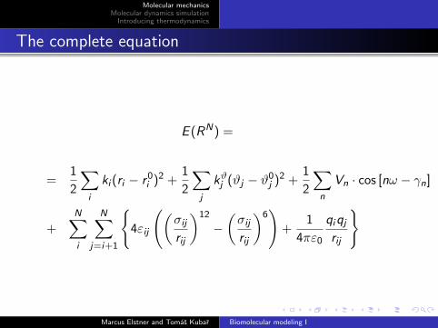
The complete equation

E (RN) =

=1

2

∑i

ki (ri − r0i )2 +

1

2

∑j

kϑj (ϑj − ϑ0j )2 +

1

2

∑n

Vn · cos [nω − γn]

+N∑i

N∑j=i+1

{4εij

((σijrij

)12

−(σijrij

)6)

+1

4πε0

qiqjrij

}




Molecular dynamics simulation

how to get things moving




Equations of motion

m · r = F

ordinary differential equations of 2nd order

have to be solved numerically

solution proceeds in discreet steps of length ∆t

numerical integration starts at time t0,where the initial conditions are specified– the positions r0 and the velocities v0

calculations of forces at r0 to get accelerations a0

then, an integrator calculates r and v at time t0 + ∆t

accelerations → step → accelerations → step → . . .




Verlet integration method

a virtual step in positive time and in ‘negative’ time,and Taylor expansion up to 2nd order:

r(t + ∆t) = r(t) + r(t) ·∆t +1

2r(t) ·∆t2

r(t −∆t) = r(t)− r(t) ·∆t +1

2r(t) ·∆t2

add both equations – eliminate the velocity r :

r(t + ∆t) = 2 · r(t)− r(t −∆t) + r(t)∆t2

r(t) = a(t) =F (t)

m= − 1

m

∂V

∂r(t)





a virtual step in positive time and in ‘negative’ time,and Taylor expansion up to 2nd order:

r(t + ∆t) = r(t) + r(t) ·∆t +1

2r(t) ·∆t2

r(t −∆t) = r(t)− r(t) ·∆t +1

2r(t) ·∆t2

add both equations – eliminate the velocity r :

r(t + ∆t) = 2 · r(t)− r(t −∆t) + r(t)∆t2

r(t) = a(t) =F (t)

m= − 1

m

∂V

∂r(t)





another but equivalent formulation – velocity Verlet

r(t + ∆t) = r(t) + v(t) ·∆t + 12a(t) ·∆t2

v(t + ∆t) = v(t) + 12 (a(t) + a(t + ∆t)) ·∆t

yet another – Leap-frog

v(t + 12 ∆t) = v(t − 1

2 ∆t) + a(t) ·∆t

r(t + ∆t) = r(t) + v(t + 12 ∆t) ·∆t




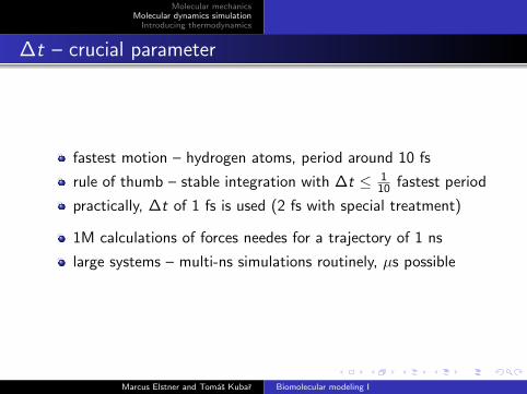
∆t – crucial parameter

Let us say: we want to obtain a trajectory over a time interval T– we perform M steps– we have to evaluate the forces on atoms M = T/∆t times

Computational cost of the calculation of forces– major computational effort– determines how many steps we can afford to make





we neglect contributions in ∆t3 and higher orders→ error per step in the order of ∆t3

keep the step short → make the error smallbut need too many steps to simulate certain time T

make the step long → cut computational costbut increase the error and decrease stability

compromise needed





fastest motion – hydrogen atoms, period around 10 fs

rule of thumb – stable integration with ∆t ≤ 110 fastest period

practically, ∆t of 1 fs is used (2 fs with special treatment)

1M calculations of forces needes for a trajectory of 1 ns

large systems – multi-ns simulations routinely, µs possible





what you simulate is what you would measure




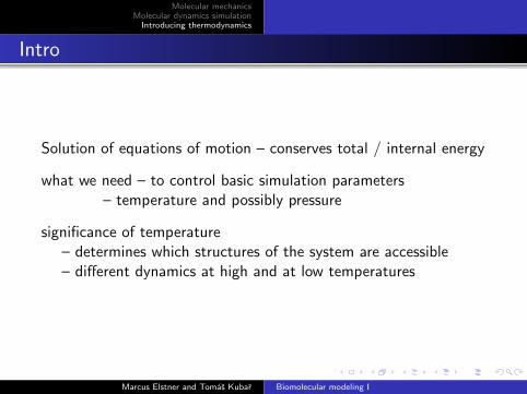
Intro

Solution of equations of motion – conserves total / internal energy

what we need – to control basic simulation parameters– temperature and possibly pressure

significance of temperature– determines which structures of the system are accessible– different dynamics at high and at low temperatures




Intro

high E – multiple different structural ‘classes’ are reachedlow E – restricted available structures

difference E − Epot corresponds to Ekin and temperature




Isolated system

exchanges with surroundings neither energy (heat / work)nor matter (particles)

total energy of system: E = Ekin + Epot = const

individually, Ekin and Epot fluctuate in the course of timeas they are being transformed into each other

is what we get when using the Verlet method for a molecule

kinetic theory of gases → relation of Ekin and temperature:

〈Ekin〉 =3

2NkT

where 〈Ekin〉 =1

2

∑i

mi

⟨v2i

⟩‘local’ T – fluctuates in time; may differ between parts of system




Isolated and closed system

experimental setup (a test tube with a sample)– usually in thermodynamic equilibrium with the surroundings– temperature (and opt. pressure) equal as that of surr.

isolated system closed system




Closed system

thermal contact of system with surroundings

exchange of energy in the form of heatuntil the temperature of surroundings is reached

canonical ensemble

velocity / speed of atoms – Maxwell–Boltzmann distribution




Canonical ensemble

Maxwell–Boltzmann distribution of velocity / speed (N2, IG)




Naıve thermostat – scaling of velocities

in a Verlet MD simulation – ‘instantaneous temperature’ Tdeviates from the target Tref (of bath = the surroundings)

T (t) =2

3

Ekin(t)

Nk6= Tref

T (t) – another name for Ekin determined by velocitiessimple idea – scale the velocities by a certain factor λ:

Tref =1

32Nk

· 1

2

∑i

mi (λ · vi )2 =

= λ2 · 132Nk

· 1

2

∑i

miv2i = λ2 · T




Naıve thermostat – scaling of velocities

scaling of all velocities by λ =√Tref/T → Tref reached exactly

rescaling the velocities affects the ‘natural’ wayof evolution of the system

velocities – not sure if the distribution is correct (M–B)

importantly, system does not sample any canonical ensemble– very important because everything is calculated as averages:

〈A〉 =1

Z

∫ρ · A d~r d~p

possibly: wrong sampling → wrong averages




Berendsen thermostat

How to avoid the drastic changes to the dynamics?adjust velocities more smoothly, in the direction of Tref

temperature changes between two time steps according to

∆T =∆t

τ(Tref − T )

rate of change of T (due to the change of velocities)is proportional to the deviation of actual T from Tref

constant of proportionality – relaxation time τ




Berendsen thermostat

velocities are scaled by λ:

Tnew = T + ∆T = T +∆t

τ(Tref − T )

λ =

√Tnew

T=

√1 +

∆t

τ

(Tref

T− 1

)usually: τ = 0.1− 10 ps

T will fluctuate around the desired value Tref

problem – still does not generate correct canonical ensemble




Nose–Hoover thermostat

represents rigorously the canonical ensemble → ideal choice

conceptionally and mathematically > difficult to understand

heat bath is treated not as an external elementrather as an integral part of the systemis assigned an additional DOF s with fictitious mass Q

eqns of motion for this extended system (3N + 1 DOF):

ri =Fimi− s · ri

s =1

Q(T − Tref)




Temperature and thermostats

fluctuation of temperature – desired propertyfor canonical ensemble – variance of ‘inst. temperature’ T :

σ2T =

⟨(T − 〈T 〉)2

⟩=⟨T 2⟩− 〈T 〉2

and relative variance

σ2T

〈T 〉2=

2

3N

large number of atoms N: fluctuations → 0finite-sized systems: visible fluctuation of temperature

– is correct (feature of the canonical ensemble)




Introducing pressure

chemical reality – constant pressure rather than constant volumegoal – implement such conditions in simulations, too

How to calculate pressure? – first, calculate virial of force

Ξ = −1

2

∑i<j

~rij · ~Fij

(~rij distance of atoms i and j , ~Fij – force between them)

P =2

3V· (Ekin − Ξ) =

2

3V·

1

2

∑i

mi · |~vi |2 +1

2

∑i<j

~rij · ~Fij




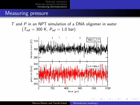
Measuring pressure

T and P in an NPT simulation of a DNA oligomer in water(Tref = 300 K, Pref = 1.0 bar)




Controlling pressure

we can calculate the pressure– so how do we maintain it at a constant value?

barostat – algorithm that is equivalent of a thermostat,just that it varies volume of the box instead of velocities

alternatives are available:

Berendsen barostat– direct rescaling of box volume– system coupled to a ‘force / pressure bath’ – piston

Parrinello–Rahman barostat– extended-ensemble simulation– additional DOF for the piston


Documents

Biomolecular modeling I - KITcbp.cfn.kit.edu/downloads/CB-praktikum-WS2015/CB-praktikum-2015-1.pdf · Simulation { we need a model to describe the interactions of atoms { the quality