Embed Size (px)
Citation preview
Enhanced samplingFree energy simulations
Modeling in the drug design
Biomolecular modeling IIII
Marcus Elstner and Tomas Kubar
2016, December 14
Marcus Elstner and Tomas Kubar Biomolecular modeling IIII
Enhanced samplingFree energy simulations
Modeling in the drug design
Enhanced sampling
How to save time, and time is money
Marcus Elstner and Tomas Kubar Biomolecular modeling IIII
Enhanced samplingFree energy simulations
Modeling in the drug design
Problem
with normal nanosecond length MD simulations:
It is difficult to overcome barriers to conformational transitions,and only conformations in the neighborhood of the initial structure
may be sampled,even if some other (different) conformations are more relevant,
i.e. have lower free energy
Special techniques are required to solve this problem.
Marcus Elstner and Tomas Kubar Biomolecular modeling IIII

Enhanced samplingFree energy simulations
Modeling in the drug design
Note – do not be afraid of Arrhenius
How often does something happen (in a simulation)?
k = A× exp [−EA/kT ], let us have A = 1× 10⁹ s−1
EA k 1/kkcal/mol 1/s µs
1 0.19× 10⁹ 0.0053 6.7× 10⁶ 0.155 0.24× 10⁶ 4.27 8.6× 10³ 120
So, if the process has to overcome a barrier of 5 kcal/mol,we will have to simulate for 4 µs to see it happen once on average.
Marcus Elstner and Tomas Kubar Biomolecular modeling IIII
Enhanced samplingFree energy simulations
Modeling in the drug design
Replica-exchange molecular dynamics
REMD (or parallel tempering) – method to accelerate the samplingof configuration space, which can be appliedeven if the configurations of interest are separated by high barriers.
Several (identical) replicas of the molecular system are simulatedat the same time, with different temperatures.
The coordinates+velocities of the replicas may be switched(exchanged) between two temperatures.
Marcus Elstner and Tomas Kubar Biomolecular modeling IIII
Enhanced samplingFree energy simulations
Modeling in the drug design
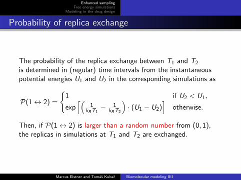
Probability of replica exchange
The probability of the replica exchange between T1 and T2
is determined in (regular) time intervals from the instantaneouspotential energies U1 and U2 in the corresponding simulations as
P(1↔ 2) =
{1 if U2 < U1,
exp[(
1kBT1
− 1kBT2
)· (U1 − U2)
]otherwise.
Then, if P(1↔ 2) is larger than a random number from (0, 1),the replicas in simulations at T1 and T2 are exchanged.
Marcus Elstner and Tomas Kubar Biomolecular modeling IIII
Enhanced samplingFree energy simulations
Modeling in the drug design
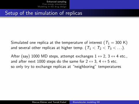
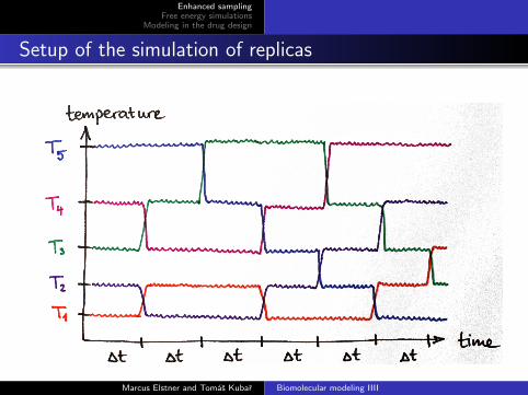
Setup of the simulation of replicas
Simulated one replica at the temperature of interest (T1 = 300 K)and several other replicas at higher temp. (T1 < T2 < T3 < . . .).
After (say) 1000 MD steps, attempt exchanges 1↔ 2, 3↔ 4 etc.,and after next 1000 steps do the same for 2↔ 3, 4↔ 5 etc.so only try to exchange replicas at “neighboring” temperatures
Marcus Elstner and Tomas Kubar Biomolecular modeling IIII
Enhanced samplingFree energy simulations
Modeling in the drug design
Setup of the simulation of replicas
Marcus Elstner and Tomas Kubar Biomolecular modeling IIII
Enhanced samplingFree energy simulations
Modeling in the drug design
Advantages of REMD
due to the simulations at high temperatures
faster sampling and more frequent crossing of energy barriers
correct sampling at all temperatures obtained,above all at the (lowest) temperature of interest
increased computational cost (multiple simulations)pays off with largely accelerated sampling
simulations running at different temperatures are independentexcept at attempted exchanges → easy parallelization
first application – protein folding (Sugita & Okamoto, Chem. Phys. Lett. 1999)
Marcus Elstner and Tomas Kubar Biomolecular modeling IIII
Enhanced samplingFree energy simulations
Modeling in the drug design
Choice of temperatures and disadvantages of REMD
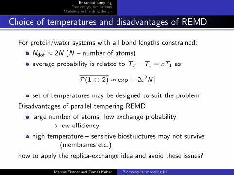
For protein/water systems with all bond lengths constrained:
Ndof ≈ 2N (N – number of atoms)
average probability is related to T2 − T1 = εT1 as
P(1↔ 2) ≈ exp[−2ε2N
]set of temperatures may be designed to suit the problem
Disadvantages of parallel tempering REMD
large number of atoms: low exchange probability→ low efficiency
high temperature – sensitive biostructures may not survive(membranes etc.)
how to apply the replica-exchange idea and avoid these issues?
Marcus Elstner and Tomas Kubar Biomolecular modeling IIII
Enhanced samplingFree energy simulations
Modeling in the drug design
Hamiltonian replica exchange – HREX
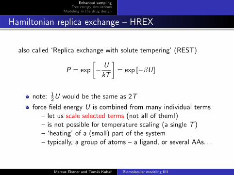
also called ‘Replica exchange with solute tempering’ (REST)
P = exp
[− U
kT
]= exp [−βU]
note: 12U would be the same as 2T
force field energy U is combined from many individual terms– let us scale selected terms (not all of them!)– is not possible for temperature scaling (a single T )– ‘heating’ of a (small) part of the system– typically, a group of atoms – a ligand, or several AAs. . .
Marcus Elstner and Tomas Kubar Biomolecular modeling IIII
Enhanced samplingFree energy simulations
Modeling in the drug design
Hamiltonian replica exchange – HREX
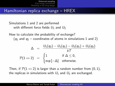
Simulations 1 and 2 are performedwith different force fields U1 and U2
How to calculate the probability of exchange?(q1 and q2 – coordinates of atoms in simulations 1 and 2)
∆ =U1(q2)− U1(q1)− U2(q1) + U2(q2)
kT
P(1↔ 2) =
{1 if ∆ ≤ 0,
exp [−∆] otherwise.
Then, if P(1↔ 2) is larger than a random number from (0, 1),the replicas in simulations with U1 and U2 are exchanged.
Marcus Elstner and Tomas Kubar Biomolecular modeling IIII
Enhanced samplingFree energy simulations
Modeling in the drug design
HREX – a good variant
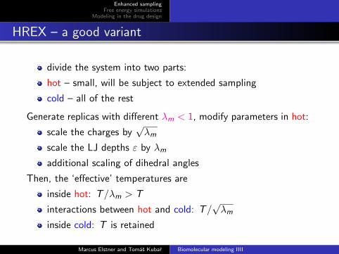
divide the system into two parts:
hot – small, will be subject to extended sampling
cold – all of the rest
Generate replicas with different λm < 1, modify parameters in hot:
scale the charges by√λm
scale the LJ depths ε by λm
additional scaling of dihedral angles
Then, the ‘effective’ temperatures are
inside hot: T/λm > T
interactions between hot and cold: T/√λm
inside cold: T is retained
Marcus Elstner and Tomas Kubar Biomolecular modeling IIII
Enhanced samplingFree energy simulations
Modeling in the drug design
HREX
Meaning of temperature
kinetic energy ← velocities– does not change, is the same in hot and cold (300 K)– simulation settings need not be adjusted (time step!)– unlike in parallel tempering
factor affecting the population of states– we play with this
Marcus Elstner and Tomas Kubar Biomolecular modeling IIII
Enhanced samplingFree energy simulations
Modeling in the drug design
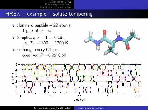
HREX – example – solute tempering
alanine dipeptide – 22 atoms,1 pair of ϕ− ψ
5 replicas, λ = 1 . . . 0.18i.e. Tm = 300 . . . 1700 K
exchange every 0.1 ps,observed P =0.25–0.50
Marcus Elstner and Tomas Kubar Biomolecular modeling IIII
Enhanced samplingFree energy simulations
Modeling in the drug design
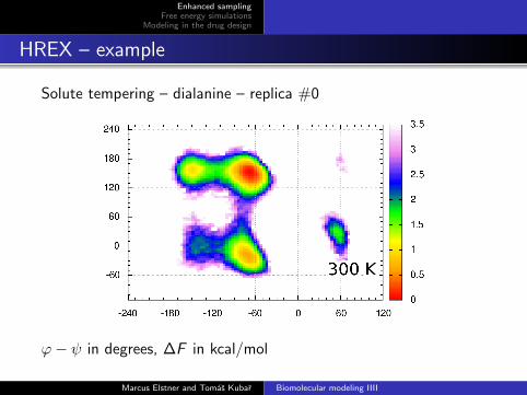
HREX – example
Solute tempering – dialanine – replica #0
ϕ− ψ in degrees, ∆F in kcal/mol
Marcus Elstner and Tomas Kubar Biomolecular modeling IIII
Enhanced samplingFree energy simulations
Modeling in the drug design
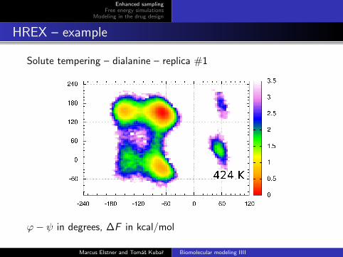
HREX – example
Solute tempering – dialanine – replica #1
ϕ− ψ in degrees, ∆F in kcal/mol
Marcus Elstner and Tomas Kubar Biomolecular modeling IIII
Enhanced samplingFree energy simulations
Modeling in the drug design
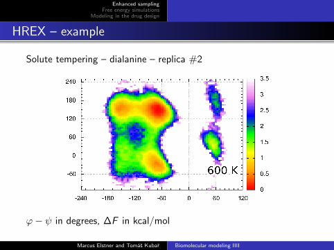
HREX – example
Solute tempering – dialanine – replica #2
ϕ− ψ in degrees, ∆F in kcal/mol
Marcus Elstner and Tomas Kubar Biomolecular modeling IIII
Enhanced samplingFree energy simulations
Modeling in the drug design
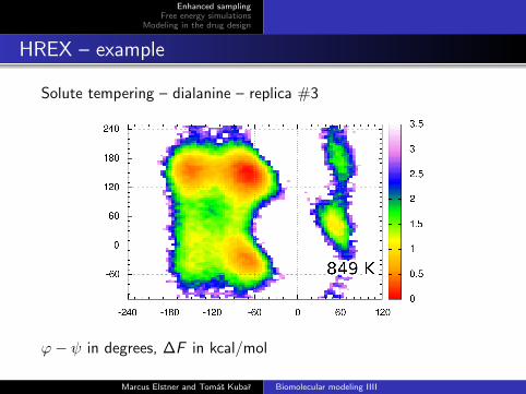
HREX – example
Solute tempering – dialanine – replica #3
ϕ− ψ in degrees, ∆F in kcal/mol
Marcus Elstner and Tomas Kubar Biomolecular modeling IIII

Enhanced samplingFree energy simulations
Modeling in the drug design
HREX – example
Solute tempering – dialanine – replica #4
ϕ− ψ in degrees, ∆F in kcal/mol
Marcus Elstner and Tomas Kubar Biomolecular modeling IIII
Enhanced samplingFree energy simulations
Modeling in the drug design
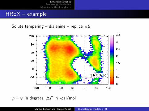
HREX – example
Solute tempering – dialanine – replica #5
ϕ− ψ in degrees, ∆F in kcal/mol
Marcus Elstner and Tomas Kubar Biomolecular modeling IIII
Enhanced samplingFree energy simulations
Modeling in the drug design
Methods using biasing potentials
Other approaches use a different idea:
It is easy to introduce an additional contributionto the potential energy of the molecule
Example – the extra potential may force the moleculeover an energy barrier, to explore other conformations
It is ‘unrealistic’ – we do not simulate a real moleculebut this bias may be removed by a right post-processing
Note: use of NMR-based distance restrains in MD simulations→ ‘NMR-refined’ structure of the molecule (e.g. PDB ID 1AC9)
Marcus Elstner and Tomas Kubar Biomolecular modeling IIII
Enhanced samplingFree energy simulations
Modeling in the drug design
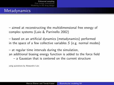
Metadynamics
– aimed at reconstructing the multidimensional free energy ofcomplex systems (Laio & Parrinello 2002)
– based on an artificial dynamics (metadynamics) performedin the space of a few collective variables S (e.g. normal modes)
– at regular time intervals during the simulation,an additional biasing energy function is added to the force field
– a Gaussian that is centered on the current structure
using quotations by Alessandro Laio
Marcus Elstner and Tomas Kubar Biomolecular modeling IIII
Enhanced samplingFree energy simulations
Modeling in the drug design
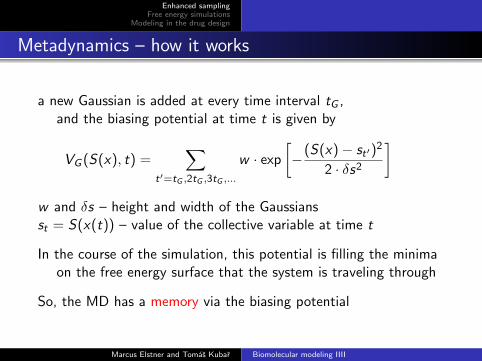
Metadynamics – how it works
a new Gaussian is added at every time interval tG ,and the biasing potential at time t is given by
VG (S(x), t) =∑
t′=tG ,2tG ,3tG ,...
w · exp
[−(S(x)− st′)
2
2 · δs2
]
w and δs – height and width of the Gaussiansst = S(x(t)) – value of the collective variable at time t
In the course of the simulation, this potential is filling the minimaon the free energy surface that the system is traveling through
So, the MD has a memory via the biasing potential
Marcus Elstner and Tomas Kubar Biomolecular modeling IIII
Enhanced samplingFree energy simulations
Modeling in the drug design
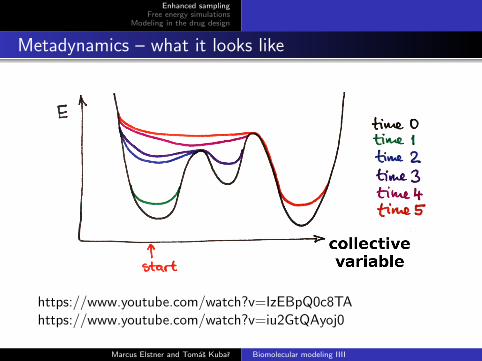
Metadynamics – what it looks like
https://www.youtube.com/watch?v=IzEBpQ0c8TAhttps://www.youtube.com/watch?v=iu2GtQAyoj0
Marcus Elstner and Tomas Kubar Biomolecular modeling IIII
Enhanced samplingFree energy simulations
Modeling in the drug design
Properties of metadynamics
Metadynamics – to explore new reaction pathways,accelerate rare events,and also to estimate the free energies efficiently.
The system escapes a local free energy minimumthrough the lowest free-energy saddle point.
The dynamics continues, and all of the free-energy profileis filled with the biasing Gaussians.
At the end, the sum of the Gaussians providesthe negative of the free energy.
Marcus Elstner and Tomas Kubar Biomolecular modeling IIII
Enhanced samplingFree energy simulations
Modeling in the drug design
Properties of metadynamics
Crucial task – prior to simulation: identify the collectivevariables of interest
that are difficult to sample because of high barriers
These variables S(x) are functions of the coordinates of the system;practical applications – up to 3 such variables,and the choice depend on the process being studied.
Typical choices – principal modes of motion obtained with PCAStill, the choice of S may be difficult
Marcus Elstner and Tomas Kubar Biomolecular modeling IIII
Enhanced samplingFree energy simulations
Modeling in the drug design
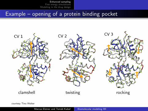
Example – opening of a protein binding pocket
clamshell twisting rocking
courtesy Tino Wolter
Marcus Elstner and Tomas Kubar Biomolecular modeling IIII
Enhanced samplingFree energy simulations
Modeling in the drug design
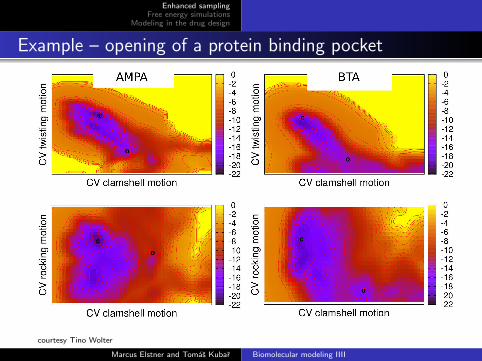
Example – opening of a protein binding pocket
courtesy Tino Wolter
Marcus Elstner and Tomas Kubar Biomolecular modeling IIII
Enhanced samplingFree energy simulations
Modeling in the drug design
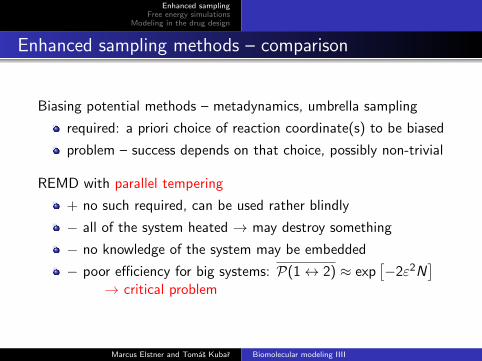
Enhanced sampling methods – comparison
Biasing potential methods – metadynamics, umbrella sampling
required: a priori choice of reaction coordinate(s) to be biased
problem – success depends on that choice, possibly non-trivial
REMD with parallel tempering
+ no such required, can be used rather blindly
− all of the system heated → may destroy something
− no knowledge of the system may be embedded
− poor efficiency for big systems: P(1↔ 2) ≈ exp[−2ε2N
]→ critical problem
Marcus Elstner and Tomas Kubar Biomolecular modeling IIII
Enhanced samplingFree energy simulations
Modeling in the drug design
Enhanced sampling methods – comparison
Hamiltonian replica exchange (HREX)
in intermediate positionbetween metadynamics/US and REMD-PT
simpler to use than metadynamics/US– results depend not so strongly on the choices to be made
efficiency does not depend on the overall system size
Marcus Elstner and Tomas Kubar Biomolecular modeling IIII
Enhanced samplingFree energy simulations
Modeling in the drug design
Free energy simulations
Marcus Elstner and Tomas Kubar Biomolecular modeling IIII
Enhanced samplingFree energy simulations
Modeling in the drug design
Motivation
physical quantities of prime interest in chemistry?
free energies – Helmholtz F or Gibbs G– determine whether processes (reactions) run spontaneously or not– holy grail of computational chemistry,
both for their importanceand because they are difficult to calculate
Marcus Elstner and Tomas Kubar Biomolecular modeling IIII
Enhanced samplingFree energy simulations
Modeling in the drug design
Convergence issue
(all of the formulas come from statistical thermodynamics)
– especially desperate for free energies:
F = kBT · ln⟨
exp
[E
kBT
]⟩serious issue – the large energy values enter an exponential,
and so the high-energy regions may contribute significantly!→ if these are undersampled, then free energies are wrong
– calculation of free energies impossible, special methods needed!
Marcus Elstner and Tomas Kubar Biomolecular modeling IIII
Enhanced samplingFree energy simulations
Modeling in the drug design
Tackling the issue
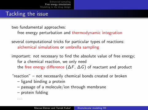
two fundamental approaches:free energy perturbation and thermodynamic integration
several computational tricks for particular types of reactions:alchemical simulations or umbrella sampling
important: not necessary to find the absolute value of free energy;for a chemical reaction, we only needthe free energy difference (∆F , ∆G ) of reactant and product
“reaction” – not necessarily chemical bonds created or broken– ligand binding a protein– passage of a molecule/ion through membrane– protein folding. . .
Marcus Elstner and Tomas Kubar Biomolecular modeling IIII
Enhanced samplingFree energy simulations
Modeling in the drug design
Thermodynamic integration
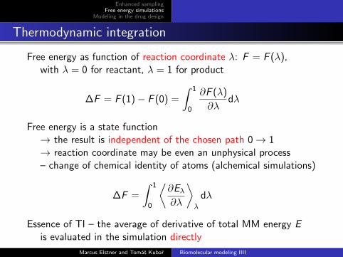
Free energy as function of reaction coordinate λ: F = F (λ),with λ = 0 for reactant, λ = 1 for product
∆F = F (1)− F (0) =
∫ 1
0
∂F (λ)
∂λdλ
Free energy is a state function→ the result is independent of the chosen path 0→ 1→ reaction coordinate may be even an unphysical process– change of chemical identity of atoms (alchemical simulations)
∆F =
∫ 1
0
⟨∂Eλ∂λ
⟩λ
dλ
Essence of TI – the average of derivative of total MM energy Eis evaluated in the simulation directly
Marcus Elstner and Tomas Kubar Biomolecular modeling IIII
Enhanced samplingFree energy simulations
Modeling in the drug design
How to do it practically
perform a MD simulation for each chosen value of λ:– usually, equidistant values in the interval (0,1) are taken:
0, 0.05, . . . , 0.95 and 1
each of these simulations produces a value of⟨∂E∂λ
⟩λ
– we obtain the derivative of F in discrete points for λ ∈ (0, 1)
this function is integrated numerically,– the result is the desired free energy difference ∆F
how many “windows”, or λ values shall we choose?– we would like to have as few windows as possible,
without compromising numerical precision– inaccuracy may be due to the numerical integration
Marcus Elstner and Tomas Kubar Biomolecular modeling IIII
Enhanced samplingFree energy simulations
Modeling in the drug design
Computational alchemy
TI looks complicated, but it is rather straightforward,– common simulation programs run TI conveniently
Computational alchemy– change of chemical identities of atoms or functional groups
Using a parameter λ, the force-field parameters of state 0are changed to those of state 1 gradually:
Eλ = (1− λ) · E0 + λ · E1
Marcus Elstner and Tomas Kubar Biomolecular modeling IIII
Enhanced samplingFree energy simulations
Modeling in the drug design
Advantages of TI
evaluate the derivative of energies,no need to sample for the (large) total energies first
it is not important what happens outside of the regionwhere the reaction takes place (no contrib. to E1 − E0)
the ensemble of structures that have to be sampled thoroughlyis much smaller, and shorter simulation length is required
Marcus Elstner and Tomas Kubar Biomolecular modeling IIII
Enhanced samplingFree energy simulations
Modeling in the drug design
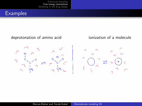
Examples
deprotonation of amino acid ionization of a molecule
Marcus Elstner and Tomas Kubar Biomolecular modeling IIII
Enhanced samplingFree energy simulations
Modeling in the drug design
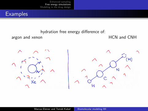
Examples
hydration free energy difference of:argon and xenon HCN and CNH
Marcus Elstner and Tomas Kubar Biomolecular modeling IIII
Enhanced samplingFree energy simulations
Modeling in the drug design
Example
The hydration free energy difference of argon and xenon
Let us interpolate between the parameters for the two elements:
ελ = (1− λ) · ε0 + λ · ε1
σλ = (1− λ) · σ0 + λ · σ1
In the simulation, we start from λ = 0, i.e. an argon atom,and change it in subsequent steps to 1.
For each step (window), we perform an MD simulationwith the corresponding values of the vdW parameters,and evaluate the free energy derivative
Marcus Elstner and Tomas Kubar Biomolecular modeling IIII
Enhanced samplingFree energy simulations
Modeling in the drug design
Example
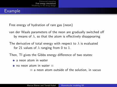
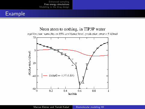
Free energy of hydration of rare gas (neon)
van der Waals parameters of the neon are gradually switched offby means of λ, so that the atom is effectively disappearing
The derivative of total energy with respect to λ is evaluatedfor 21 values of λ ranging from 0 to 1.
Then, TI gives the Gibbs energy difference of two states:
a neon atom in water
no neon atom in water ≡≡ a neon atom outside of the solution, in vacuo
Marcus Elstner and Tomas Kubar Biomolecular modeling IIII
Enhanced samplingFree energy simulations
Modeling in the drug design
Example
Marcus Elstner and Tomas Kubar Biomolecular modeling IIII
Enhanced samplingFree energy simulations
Modeling in the drug design
Differences of differences
Often – we are interested not in the absolute free energiesand not even in the reaction free energies,
rather, in the difference (∆) of reaction free energies (∆F )of two similar reactions:
∆∆F or ∆∆G
Marcus Elstner and Tomas Kubar Biomolecular modeling IIII
Enhanced samplingFree energy simulations
Modeling in the drug design
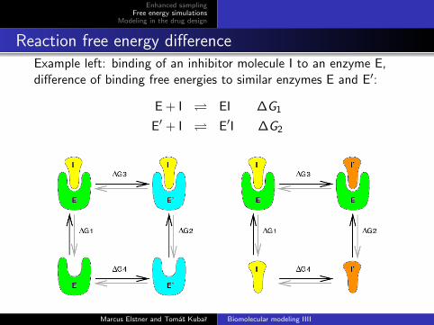
Reaction free energy differenceExample left: binding of an inhibitor molecule I to an enzyme E,difference of binding free energies to similar enzymes E and E′:
E + I EI ∆G1
E′ + I E′I ∆G2
Marcus Elstner and Tomas Kubar Biomolecular modeling IIII
Enhanced samplingFree energy simulations
Modeling in the drug design
Reaction free energy difference
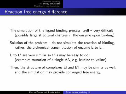
The simulation of the ligand binding process itself – very difficult(possibly large structural changes in the enzyme upon binding)
Solution of the problem – do not simulate the reaction of binding,rather, the alchemical transmutation of enzyme E to E′.
E to E′ are very similar so this may be easy to do.(example: mutation of a single AA, e.g. leucine to valine)
Then, the structure of complexes EI and E′I may be similar as well,and the simulation may provide converged free energy.
Marcus Elstner and Tomas Kubar Biomolecular modeling IIII
Enhanced samplingFree energy simulations
Modeling in the drug design
Reaction free energy difference
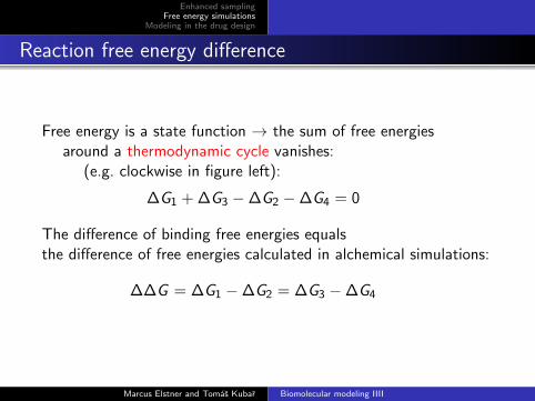
Free energy is a state function → the sum of free energiesaround a thermodynamic cycle vanishes:
(e.g. clockwise in figure left):
∆G1 + ∆G3 −∆G2 −∆G4 = 0
The difference of binding free energies equalsthe difference of free energies calculated in alchemical simulations:
∆∆G = ∆G1 −∆G2 = ∆G3 −∆G4
Marcus Elstner and Tomas Kubar Biomolecular modeling IIII
Enhanced samplingFree energy simulations
Modeling in the drug design
Geometric reaction coordinate
Sometimes, we need to know how the free energy changesalong a geometric reaction coordinate q
The free energy is then a function of q
Such a function F (q) is called the potential of mean force.
Examples:
distance between two particles in a dissociating complex
the position of a proton for a reaction of proton transfer
the dihedral angle when dealing with conformational changes
Marcus Elstner and Tomas Kubar Biomolecular modeling IIII
Enhanced samplingFree energy simulations
Modeling in the drug design
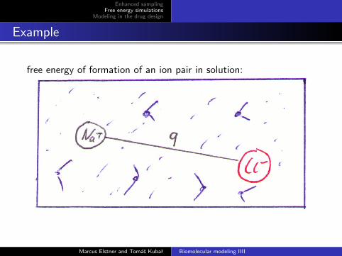
Example
free energy of formation of an ion pair in solution:
Marcus Elstner and Tomas Kubar Biomolecular modeling IIII
Enhanced samplingFree energy simulations
Modeling in the drug design
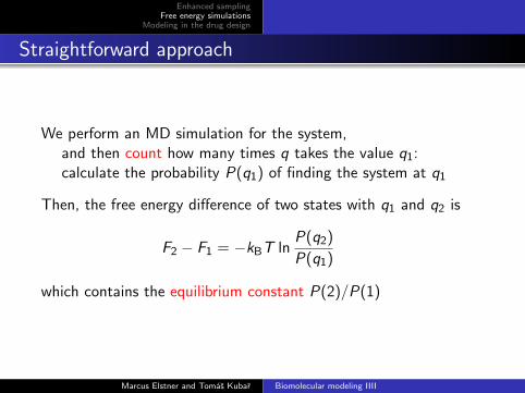
Straightforward approach
We perform an MD simulation for the system,and then count how many times q takes the value q1:calculate the probability P(q1) of finding the system at q1
Then, the free energy difference of two states with q1 and q2 is
F2 − F1 = −kBT lnP(q2)
P(q1)
which contains the equilibrium constant P(2)/P(1)
Marcus Elstner and Tomas Kubar Biomolecular modeling IIII

Enhanced samplingFree energy simulations
Modeling in the drug design
The problem:If a high barrier has to be crossed to come from A to B,a pure (unbiased) MD simulation will hardly make it→ the high-energy region (barrier) is described poorly (for sure)→ we may not obtain the product at all (possibly)
Marcus Elstner and Tomas Kubar Biomolecular modeling IIII
Enhanced samplingFree energy simulations
Modeling in the drug design
Working principle
Apply an additional potential, also called biasing potentialto restrain the system to values of reaction coordinatethat would otherwise remain undersampled.
This is the principle of the umbrella sampling.
The additional potential will become a part of the force field,and it shall depend only on the reaction coordinate: V = V (q)
Marcus Elstner and Tomas Kubar Biomolecular modeling IIII
Enhanced samplingFree energy simulations
Modeling in the drug design
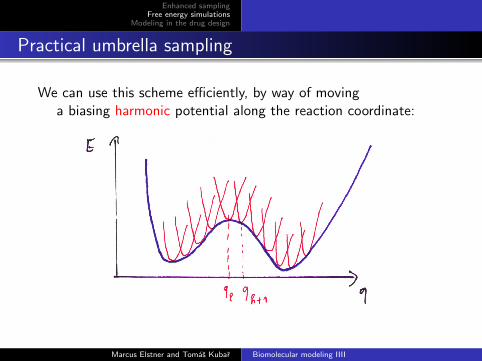
Practical umbrella sampling
We can use this scheme efficiently, by way of movinga biasing harmonic potential along the reaction coordinate:
Marcus Elstner and Tomas Kubar Biomolecular modeling IIII
Enhanced samplingFree energy simulations
Modeling in the drug design
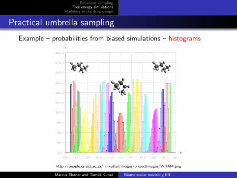
Practical umbrella sampling
Example – probabilities from biased simulations – histograms
http://people.cs.uct.ac.za/˜mkuttel/images/projectImages/WHAM.png
Marcus Elstner and Tomas Kubar Biomolecular modeling IIII
Enhanced samplingFree energy simulations
Modeling in the drug design
Potentials of mean force
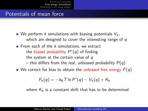
We perform k simulations with biasing potentials Vk ,which are designed to cover the interesting range of q
From each of the k simulations, we extractthe biased probability P∗(q) of findingthe system at the certain value of q– this differs from the real, unbiased probability P(q)
We correct for bias to obtain the unbiased free energy F (q)
Fk(q) = −kBT lnP∗(q)− Vk(q) + Kk
where Kk is a constant shift that has to be determined
Marcus Elstner and Tomas Kubar Biomolecular modeling IIII
Enhanced samplingFree energy simulations
Modeling in the drug design
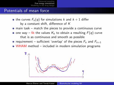
Potentials of mean force
the curves Fk(q) for simulations k and k + 1 differby a constant shift, difference of K
main task – match the pieces to provide a continuous curve
one way – fit the values Kk to obtain a resulting F (q) curvethat is as continuous and smooth as possible
requirement – sufficient ‘overlap’ of the pieces Fk and Fk+1
WHAM method – included in modern simulation programs
Marcus Elstner and Tomas Kubar Biomolecular modeling IIII
Enhanced samplingFree energy simulations
Modeling in the drug design
Molecular modeling in the drug design
Marcus Elstner and Tomas Kubar Biomolecular modeling IIII
Enhanced samplingFree energy simulations
Modeling in the drug design
Drug design
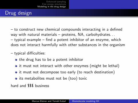
– to construct new chemical compounds interacting in a definedway with natural materials – proteins, NA, carbohydrates. . .– typical example – find a potent inhibitor of an enzyme, whichdoes not interact harmfully with other substances in the organism
– typical difficulties:
the drug has to be a potent inhibitor
it must not interact with other enzymes (might be lethal)
it must not decompose too early (to reach destination)
its metabolites must not be (too) toxic
hard and $$$ business
Marcus Elstner and Tomas Kubar Biomolecular modeling IIII
Enhanced samplingFree energy simulations
Modeling in the drug design
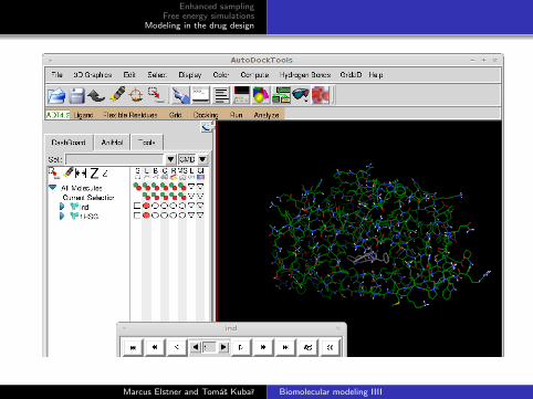
Molecular docking
“Docking is a method which predicts the preferred orientationof one molecule to a second when bound to each otherto form a stable complex.” Wikipedia
Typical pharmacological problem – find a ligand molecule to bindto a protein as strongly and specifically as possible
Good news: the binding site (pocket) is usually known– often, the active or allosteric place of the protein
Bad news:
many DoF – transl., rot. and internal flex. of the ligand
only a small number of molecules can be docked manually,once the binding mode of a similar molecule is known(and, even similar molecules sometimes bind differently)
Marcus Elstner and Tomas Kubar Biomolecular modeling IIII
Enhanced samplingFree energy simulations
Modeling in the drug design
Molecular docking
a sequence of tasks:
1 Generate the pool of compounds to test – database ofcompounds, construction from a database of moieties,. . .
2 For each compound, find the binding mode. For this,try out several/many orientations and conformations (poses),and determine the most favorable
3 Evaluate the strength of the interaction.Accurate determination of ∆Gbind impossible;instead, a scoring function is employed
Marcus Elstner and Tomas Kubar Biomolecular modeling IIII
Enhanced samplingFree energy simulations
Modeling in the drug design
Molecular docking
Various levels of approximation may be employed
The simplest approach – exploit a database of molecules, andtry to fit each molecule as a rigid body into the binding pocketA natural expansion – consider the flexibility of the ligand
How to generate different configurations of the molecule?
simple minimization or molecular dynamics
Monte Carlo, perhaps combined with simulated annealing
genetic algorithms
Efficient alternative – incremental construction of the ligand,which is partitioned into chemically reasonable fragments
– natural account for the conformational flexibility of the molecule
Marcus Elstner and Tomas Kubar Biomolecular modeling IIII
Enhanced samplingFree energy simulations
Modeling in the drug design
Molecular docking
problem of docking – it is all about sampling
No way to do molecular dynamics for every candidate molecule:
MD takes much longer than what is affordable(would be OK for one ligand, but there are too many)
MD would probably work only for quite rigid molecules movingrelatively freely in the binding pocket (usually not the case)
Difference:
If the goal is to dock a single molecule – a thorough search isaffordable, involving MD, enhanced sampling. . .
If we have to dock and assess many candidate ligands– simpler approaches have to be chosen– current state of the art – consider the flexibility of ligands– flexibility of protein (side chains) under development
Marcus Elstner and Tomas Kubar Biomolecular modeling IIII
Enhanced samplingFree energy simulations
Modeling in the drug design
Scoring function
needed: extremely efficient way to quantify the strength of binding
1 to find the right binding mode of each ligand
2 to compare the strength of binding of various ligands.
the quantity of interest – binding free energyproblem with free energy methods – too inefficient for dockingwhat we need here – a simple additive function to approximate∆Gbind, which would give a result rapidly, in a single step
Marcus Elstner and Tomas Kubar Biomolecular modeling IIII
Enhanced samplingFree energy simulations
Modeling in the drug design
Scoring function
∆Gbind = ∆Gsolv + ∆Gconf + ∆Gint + ∆Grot + ∆Gt/r + ∆Gvib
∆Gsolv – change of hydration (ligand, protein) upon binding∆Gconf – deformation energy of the ligand (forced by the pocket)∆Gint – ‘interaction energy’ – a favorable contribution
due to the specific ligand–protein interactions∆Grot – loss of entropy due to the frozen rotationsapprox. +RT log 3 = 0.7 kcal/mol per 3-state rotatable bond∆Gt/r – loss of trans. and rot. entropy upon association
– approx. the same for all ligands of similar size∆Gvib – change of vibrational modes – difficult, often ignored
Marcus Elstner and Tomas Kubar Biomolecular modeling IIII
Enhanced samplingFree energy simulations
Modeling in the drug design
Scoring function
a ‘force field’ for the free energy of binding
problem – although approximative, it is still too costly
usually, very simple constructions, looking over-simplified incomparison with MM force fields; example (Bohm, 1994):
∆G = ∆G0 + ∆GHbond ·∑
Hbonds
f (R, α) + ∆Gionpair ·∑
ionpairs
f ′(R, α)
+ ∆Glipo · Alipo + ∆Grot · Nrot
∆GHbond – ideal hydrogen bondf (R, α) – penalty function for a realistic hydrogen bond∆Gionpair and f ′(R, α) – dtto for ionic contacts∆Glipo – due to hydrophobic interaction; non-polar SA Alipo
∆Grot – due to a rotatable bond that freezes upon binding
Marcus Elstner and Tomas Kubar Biomolecular modeling IIII
Enhanced samplingFree energy simulations
Modeling in the drug design
Scoring function
Further concepts present in other scoring functions:
partitioning of the surface areas of both the proteins and theligand into polar and non-polar regions, and assigningdifferent parameters to the interactions of different kinds ofregions (polar-polar, polar-nonpolar, nonpolar-nonpolar)
statistical techniques to parametrize the scoring function
Problem – such s.f. only describe well ligands that bind tightlyModestly binding ligands
– of increasing interest in docking studies– more poorly described by such functions
Possible solution – ‘consensus scoring’ – combining results fromseveral scoring functions; performs better than any single s.f.
Marcus Elstner and Tomas Kubar Biomolecular modeling IIII
Enhanced samplingFree energy simulations
Modeling in the drug design
Scoring function
Comment on accuracy
an error of ∆Gbind of 1.4 kcal/mol→ ten-fold increase/decrease of the inhibition constant
or: as little as 4.2 kcal/mol of ∆Gbind liesbetween a micro- and a nanomolar inhibitor
Therefore, the requirements on the accuracy of s.f.are actually rather big
Marcus Elstner and Tomas Kubar Biomolecular modeling IIII
Enhanced samplingFree energy simulations
Modeling in the drug design
Marcus Elstner and Tomas Kubar Biomolecular modeling IIII
Enhanced samplingFree energy simulations
Modeling in the drug design
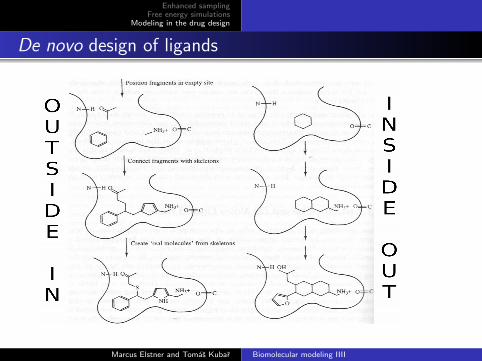
De novo design of ligands
It may be a good idea to construct the ligand ‘from scratch’– without relying on the content of a database.
2 basic types of de novo design:
outside–in: Binding site is analyzed and tightly-binding ligandfragments are proposed. They are connected (db of linkers)→ molecular skeleton of the ligand → actual molecule.
inside–out: ‘growing’ the ligand in the binding pocket, drivenby a search algorithm with a scoring function.
Marcus Elstner and Tomas Kubar Biomolecular modeling IIII
Enhanced samplingFree energy simulations
Modeling in the drug design
De novo design of ligands
Marcus Elstner and Tomas Kubar Biomolecular modeling IIII
Enhanced samplingFree energy simulations
Modeling in the drug design
Molecular docking
Glossary of terms
receptor / host / lock
ligand / guest / key
docking
binding mode – position and orientation of ligand
pose – a candidate for the binding mode
scoring – determine how favorable a pose is
ranking – of the poses to determine the binding mode
Marcus Elstner and Tomas Kubar Biomolecular modeling IIII