BIOSTATISTICS FOR THE CLINICIAN - Pharmaceutical · PDF file183 Biostatistics for the Clinician Learning Objectives 1. Understand when to use and how to calculate and interpret different

Biostatistics for the Clinician183

Learning Objectives1. Understand when to use and how to calculate and

interpret different measures of central tendency (mean,median, and mode) and dispersion (range, interquartilerange [IR], and standard deviation [SD]).

2. Identify the types of error encountered in statisticalanalysis, the role of sample size, effect size, variability,and power in their occurrence, and implications fordecision making.

3. Describe basic assumptions required for utilization ofcommon statistical tests including the Student’s t-test,paired t-test, Chi square analysis, Fisher’s exact test,Mann-Whitney U test, Wilcoxon signed rank, log ranktest, and Cox Proportional Hazards model.

4. Understand the common statistical tests used foranalyzing multiple variables, including one-way andtwo-way (repeated measures) analysis of variance.

5. Interpret a confidence interval (CI) with inferentialfunctions.

6. Differentiate between association and correlationanalysis, interpret correlation coefficients andregression coefficients, and describe the application ofsingle and multivariable statistical models.

7. Describe and interpret common statistical techniquesused in performing meta-analysis.

IntroductionPharmacists need to have a basic understanding of

statistical concepts to critically evaluate the literature and

determine if and how information from a study can beapplied to an individual patient. By using data fromwell-designed studies that have been appropriately analyzedand interpreted, clinicians are able to determine how the“average patient” might respond to a new medication. Theproblem of course, is how many times do clinicians care for“average patients”? Statistics would be much lesssophisticated if every individual were alike; response totherapy would be highly predictable. The science ofstatistics allows clinicians to describe the profile of theaverage person, then estimate how well that profile matchesthat of others in the population under consideration.Statistics do not tell the reader of the clinical relevance ofdata. When a difference is considered to be statisticallysignificant, the reader rejects the null hypothesis, and statethat there is a low probability of getting a result as extremeas the one observed with the data. Clinicians need tointerpret this data and to guide the clinical decision-makingprocess (i.e., the decision to use or not use a medication fora specific patient). By staying current with the literature andcritically evaluating new scientific advancements, cliniciansare able to make educated decisions regarding how to carefor patients.

Several published studies have critiqued the selectionand application of statistics in the medical literature. Thesearticles, many in well-respected medical journals, haveconsistently found high rates of inappropriate application,reporting, and interpretation of statistical information.Although it is critical to collaborate with a biostatistician inall phases of research, it is not necessary to be a statisticianto present or interpret basic statistics appropriately. Thischapter provides an overview of basic concepts related to

BIOSTATISTICS FOR THECLINICIAN

Pharmacotherapy Self-Assessment Program, 4th Edition

Mary Lea Harper, Pharm.D.

“0” and male patients as “1”. The ordering is arbitrary andno information is gained or lost because of the order. Theconclusions that are drawn will be identical regardless ofthe ordering of the samples. Nominal data are described byusing frequencies (e.g., percent of females).

Ordinal variables are also sorted into mutually exclusivegroups based on some common characteristic that allmembers of the group possess. However, unlike nominaldata, ordinal data are sorted by categories often withnumbers denoting a rank order. Again, whether numbersare assigned to these values is irrelevant. Ordinal data areused when the relative degree of presence or absence of acertain characteristic can be measured qualitatively, notquantitatively. The magnitude of difference is eitherunequal or unknown. The type of data is often collected

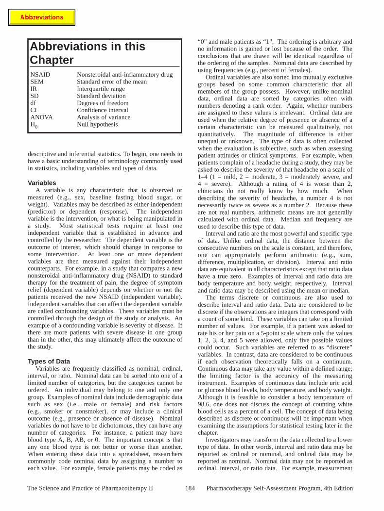
NSAID Nonsteroidal anti-inflammatory drugSEM Standard error of the meanIR Interquartile rangeSD Standard deviationdf Degrees of freedomCI Confidence intervalANOVA Analysis of varianceH0 Null hypothesis

Abbreviations in thisChapter

descriptive and inferential statistics. To begin, one needs tohave a basic understanding of terminology commonly usedin statistics, including variables and types of data.

Variables A variable is any characteristic that is observed or

measured (e.g., sex, baseline fasting blood sugar, orweight). Variables may be described as either independent(predictor) or dependent (response). The independentvariable is the intervention, or what is being manipulated ina study. Most statistical tests require at least oneindependent variable that is established in advance andcontrolled by the researcher. The dependent variable is theoutcome of interest, which should change in response tosome intervention. At least one or more dependentvariables are then measured against their independentcounterparts. For example, in a study that compares a newnonsteroidal anti-inflammatory drug (NSAID) to standardtherapy for the treatment of pain, the degree of symptomrelief (dependent variable) depends on whether or not thepatients received the new NSAID (independent variable).Independent variables that can affect the dependent variableare called confounding variables. These variables must becontrolled through the design of the study or analysis. Anexample of a confounding variable is severity of disease. Ifthere are more patients with severe disease in one groupthan in the other, this may ultimately affect the outcome ofthe study.

Types of Data Variables are frequently classified as nominal, ordinal,

interval, or ratio. Nominal data can be sorted into one of alimited number of categories, but the categories cannot beordered. An individual may belong to one and only onegroup. Examples of nominal data include demographic datasuch as sex (i.e., male or female) and risk factors(e.g., smoker or nonsmoker), or may include a clinicaloutcome (e.g., presence or absence of disease). Nominalvariables do not have to be dichotomous, they can have anynumber of categories. For instance, a patient may haveblood type A, B, AB, or 0. The important concept is thatany one blood type is not better or worse than another.When entering these data into a spreadsheet, researcherscommonly code nominal data by assigning a number toeach value. For example, female patients may be coded as

when the evaluation is subjective, such as when assessingpatient attitudes or clinical symptoms. For example, whenpatients complain of a headache during a study, they may beasked to describe the severity of that headache on a scale of1–4 (1 = mild, 2 = moderate, 3 = moderately severe, and4 = severe). Although a rating of 4 is worse than 2,clinicians do not really know by how much. Whendescribing the severity of headache, a number 4 is notnecessarily twice as severe as a number 2. Because theseare not real numbers, arithmetic means are not generallycalculated with ordinal data. Median and frequency areused to describe this type of data.

Interval and ratio are the most powerful and specific typeof data. Unlike ordinal data, the distance between theconsecutive numbers on the scale is constant, and therefore,one can appropriately perform arithmetic (e.g., sum,difference, multiplication, or division). Interval and ratiodata are equivalent in all characteristics except that ratio datahave a true zero. Examples of interval and ratio data arebody temperature and body weight, respectively. Intervaland ratio data may be described using the mean or median.

The terms discrete or continuous are also used todescribe interval and ratio data. Data are considered to bediscrete if the observations are integers that correspond witha count of some kind. These variables can take on a limitednumber of values. For example, if a patient was asked torate his or her pain on a 5-point scale where only the values1, 2, 3, 4, and 5 were allowed, only five possible valuescould occur. Such variables are referred to as “discrete”variables. In contrast, data are considered to be continuousif each observation theoretically falls on a continuum.Continuous data may take any value within a defined range;the limiting factor is the accuracy of the measuringinstrument. Examples of continuous data include uric acidor glucose blood levels, body temperature, and body weight.Although it is feasible to consider a body temperature of98.6, one does not discuss the concept of counting whiteblood cells as a percent of a cell. The concept of data beingdescribed as discrete or continuous will be important whenexamining the assumptions for statistical testing later in thechapter.

Investigators may transform the data collected to a lowertype of data. In other words, interval and ratio data may bereported as ordinal or nominal, and ordinal data may bereported as nominal. Nominal data may not be reported asordinal, interval, or ratio data. For example, measurement

184The Science and Practice of Pharmacotherapy II Pharmacotherapy Self-Assessment Program, 4th Edition

185

of blood pressure is normally collected using an intervalscale. It could also be reported as follows:

� 90 mm Hg 10 patients> 90 mm Hg 16 patients

In this example, data from patients are inserted into one oftwo mutually exclusive categories. It is not possible forpatients to fit into more than one category. The occurrenceof one event excludes the possibility of the other event. Thisis an example of how nominal data can be presented. It isgenerally undesirable to transform data to a lower levelbecause information is lost when individuals are collectivelyincluded in more general categories. If data are transformed,it should be presented in both ways. For instance, in thepresentation of blood pressure measurements, it may beworthwhile to present the mean change in blood pressure(ratio data), as well as the numbers of patients that achievegoal blood pressure values (nominal data).

Descriptive Versus Inferential Statistics Descriptive statistics are concerned with the presentation,

organization, and summarization of data. In contrast,inferential statistics are used to generalize data from oursample to a larger group of patients. A population is definedas the total group of individuals having a particularcharacteristic (e.g., all children in the world with asthma).A population is rarely available to study as it is usuallyimpractical to test every member of the population.Therefore, inferences are made from taking a randomizedsample of the population. A sample is a subset of thepopulation. Inferential statistics require that the sampling berandom; that is, each patient has an equal chance ofreceiving either treatment. Some types of sampling seek tomake the sample as representative of the population aspossible by choosing the sample to resemble the populationon the most important characteristics (surveys for assessingmedication histories relating to risk of side effects). Forinstance, when investigators study a new NSAID in 50geriatric patients with osteoarthritis, they are not justinterested in how these patients in the study respond, butrather they are interested in how to treat all geriatricindividuals with osteoarthritis. Thus, they are trying tomake inferences from a small group of patients (sample) toa larger group (population).

Frequency Distribution Data can be organized and presented in such a way that

allows an investigator to get a visual perspective of the data.This is accomplished by constructing a frequencydistribution. These distributions may be described by thecoefficient of skewness or kurtosis. Skewness is a measureof symmetry of a curve. A distribution is skewed to theright (positive skew) when the mode and median are lessthan the mean. A distribution that is skewed to the left(negative skew) is one in which the mode and median aregreater than the mean. The direction of the skew refers tothe direction of the longer tail. Kurtosis refers to how flat(platykurtic) or peaked (leptokurtic) the curve appears. Thefrequency distribution histogram (i.e., a type of bar graph

representing an entire set of data) is often a symmetric,bell-shaped curve referred to as a normal distribution (alsoreferred to as Gaussian curve, curve of error, and normalprobability curve). Under these circumstances (i.e., normaldistribution), the mean, median, and mode are all similar,and the kurtosis is zero. The mean plus one standarddeviation (SD) includes approximately 68% of the data.The assumption that there is normal distribution of variablesin the population is important because the data are easy tomanipulate. Several powerful statistical tests (e.g. Student’st-test, as well as other parametric tests) require a normaldistribution of data. However, the Student’s t test and otherparametric tests assume rather than require normaldistributions. The central limit theorem states that given adistribution with a mean (m) and variance (s2) the samplingdistribution of the mean approaches a normal distributionwith a mean (m) and a variance (s2)/N as N (sample size)increases. This assumption is based on the premise thatwhen equally sized samples are drawn from a non-normaldistribution from the same population, the mean values fromthe samples will form a normal distribution, regardless ofthe shape of the original distribution. For mostdistributions, a normal distribution is approached veryquickly as the sample increases (e.g., N>30).

Mean, Median, and Mode There are three generally accepted measures of central

tendency (also referred to as location): the mean, median,and mode. The mean (denoted by ) is one acceptablemeasure of central tendency for interval and ratio data(Table 1-1). It is defined by the summation of all values(denoted by X for each data point) divided by the number ofsubjects in the sample (n) and can be described by theequation

= ∑x/n.

For instance, the mean number of seizures during a24-hour period in seven patients with the following values9, 3, 9, 7, 8, 2, 5, is calculated by dividing the sum of 43 by7, which is equal to 6.14, or an average of approximately sixseizures per patient.

The median is the value where half of the data points fallabove and half below it. It is also referred to as the 50thpercentile. It is an appropriate measure of central tendencyfor interval, ratio, and ordinal data. When calculating themedian, the first step is to put the values in rank order. Forexample, the median number of seizures during a 24-hourperiod in seven patients with the following values 2, 3, 5, 7,8, 9, 9 is 7. There are three values below and three valuesabove the number 7. If we added one more value (e.g., 11),the median would be calculated by taking the two middlenumbers and dividing by two. Under these circumstances,the calculation would change to (7 + 8)/2 to get a median of7.5. Half of the numbers are below 7.5 and half are above.The median has an advantage over mean in that it is affectedless by outliers in the data. An outlier is a data point that isan extreme value either much lower or higher than the restof the values in the data set. Mathematically, outliers can bedetermined by using the following formulas: values greaterthan 1.5 times the interquartile range (IR) plus the upper

Biostatistics for the ClinicianPharmacotherapy Self-Assessment Program, 4th Edition

quartile or values less than the lower quartile minus1.5 times the IR are often considered outliers. A moreextensive description of IR is described below.

The measure of central tendency for nominal data is themode. The mode is the most frequently occurring numberin a dataset. The mode of the above series of numbers is 9.The mode is not frequently presented in clinical trials unlessa large data set is described.

Measures of Dispersion—Range, InterquartileRange, and Standard Deviation

The measure of dispersion (also referred to as measuresof variability or spread) describes how closely the datacluster around the measure of central tendency. Data pointsthat are scattered close to the measure of central tendencygive a different perspective than those not as close to thevalue. For instance, the mean may be seemingly verydifferent between two groups, but when examining datawith a large amount of variability around the mean, theymay begin to look similar. There are three commonmeasures of dispersion: the range, IR, and SD. The rangeis defined as the difference between the highest and lowestvalues. If we had the same numbers as above (i.e., 2, 3, 5,7, 8, 9, 9) to describe the total number of seizures atbaseline, the range of values is 9-2 or 7. Frequently, whenpresenting data in clinical trials, investigators will describethis data as “9-2”, and not use the single number. Thisprovides more information about the sample. There is anadvantage in providing the mean plus the range overproviding the mean alone. For instance, a mean age of 50 ina study without a measure of dispersion gives a differentsense of the data than when you tell individuals that therange included individuals from 12 to 78 years of age. Thistells the reader that data were obtained from both theadolescent and geriatric populations. The disadvantage ofthe range over other measures of dispersion is that it isgreatly affected by outliers. In the above example, if therewas only one 12 year old in the study, and the next youngestindividual in the study was 47, the range was greatlyaffected by this one outlier.

The IR is another measure of spread or dispersion. Thelower quartile is also referred to as the 25th percentile andthe upper quartile is the 75th percentile. The IR is defined

as the difference between the lower quartile (often referredto as Q1) and the upper quartile (often referred to as Q3) andcomprises the middle 50% of the data. The formula for theIR is Q3 - Q1. To determine the IR, the numbers are againsorted in rank order. Consider the following example ofnumber of seizures:

In this example, the first quartile is 3, the second quartile(which is the median) is 7, and the third quartile is 9. TheIR is 3 to 9. Although the IR is not used extensively, it isconsidered to be underutilized because it is considereda stable measure of spread.

The SD is the most widely used measure of dispersion. Itis defined as an index of the degree of variability of studydata about the mean. For example, assume you need todetermine what the mean and SD for the following data setof scores on a test are: 56, 62, 52, 50, and 45. The samplemean is 53 mm Hg (56 + 62 + 52 + 50 + 45)/5. Thedeviations are calculated in Table 1-2.

The sum of the deviations will always be zero. When thesum of the squared differences between the individualobservations and the mean is computed, and this value isdivided by the degrees of freedom (df), it produces anintermediate measure known as the sample variance (s2).The degrees of freedom (n-1) are used in this equation tocorrect for bias in the results that would occur if just the

2 3 5 7 8 9 9Q1 Q2 Q3


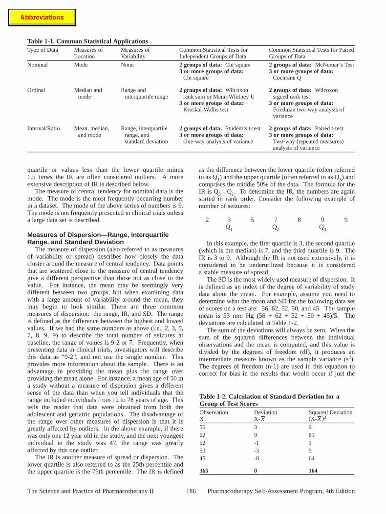
Table 1-1. Common Statistical ApplicationsType of Data Measures of Measures of Common Statistical Tests for Common Statistical Tests for Paired

Location Variability Independent Groups of Data Groups of Data

Nominal Mode None 2 groups of data: Chi square 2 groups of data: McNemar’s Test 3 or more groups of data: 3 or more groups of data:

Chi square Cochrane Q

Ordinal Median and Range and 2 groups of data: Wilcoxon 2 groups of data: Wilcoxonmode interquartile range rank sum or Mann-Whitney U signed rank test

3 or more groups of data: 3 or more groups of data:Kruskal-Wallis test Friedman two-way analysis of

variance

Interval/Ratio Mean, median, Range, interquartile 2 groups of data: Student’s t-test 2 groups of data: Paired t-testand mode range, and 3 or more groups of data: 3 or more groups of data:

standard deviation One-way analysis of variance Two-way (repeated measures)analysis of variance

Table 1-2. Calculation of Standard Deviation for aGroup of Test ScoresObservation Deviation Squared DeviationX X- (X- )2

56 3 962 9 8152 -1 150 -3 945 -8 64

365 0 164

187

number of observations (n) was used. In general, thedegrees of freedom of an estimate are equal to the numberof independent scores that go into the estimate minus thenumber of parameters estimated. If the average squareddeviation was divided by n observations, the variance wouldbe underestimated. As the size of the sample of dataincreases, the effect of dividing by n or n-1 is negligible.The sample SD, equal to the square root of the variance, isdenoted by the letter s as defined by the following formula:

∑(X- )2s = n-1

Using this formula, the SD is the square root of 164/4 or6.4. From this example, one can see that each deviationcontributes to the SD. Thus, a sample of the same size withless dispersion will have a smaller SD. For example, if thedata were changed to: 55, 52, 53, 55, and 50, the mean is thesame, but the SD is smaller because the observations liecloser to the mean.

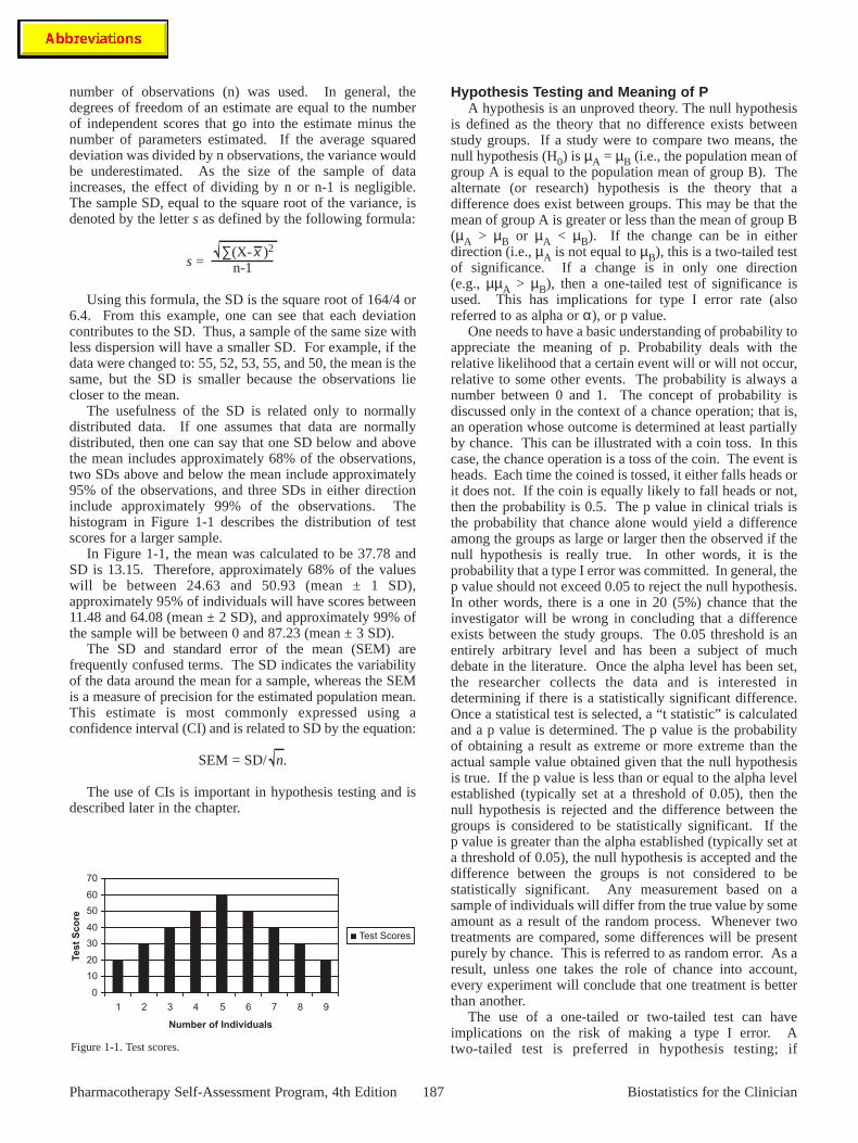
The usefulness of the SD is related only to normallydistributed data. If one assumes that data are normallydistributed, then one can say that one SD below and abovethe mean includes approximately 68% of the observations,two SDs above and below the mean include approximately95% of the observations, and three SDs in either directioninclude approximately 99% of the observations. Thehistogram in Figure 1-1 describes the distribution of testscores for a larger sample.

In Figure 1-1, the mean was calculated to be 37.78 andSD is 13.15. Therefore, approximately 68% of the valueswill be between 24.63 and 50.93 (mean ± 1 SD),approximately 95% of individuals will have scores between11.48 and 64.08 (mean ± 2 SD), and approximately 99% ofthe sample will be between 0 and 87.23 (mean ± 3 SD).

The SD and standard error of the mean (SEM) arefrequently confused terms. The SD indicates the variabilityof the data around the mean for a sample, whereas the SEMis a measure of precision for the estimated population mean.This estimate is most commonly expressed using aconfidence interval (CI) and is related to SD by the equation:

SEM = SD/ n.

The use of CIs is important in hypothesis testing and isdescribed later in the chapter.

Hypothesis Testing and Meaning of P A hypothesis is an unproved theory. The null hypothesis

is defined as the theory that no difference exists betweenstudy groups. If a study were to compare two means, thenull hypothesis (H0) is µA = µB (i.e., the population mean ofgroup A is equal to the population mean of group B). Thealternate (or research) hypothesis is the theory that adifference does exist between groups. This may be that themean of group A is greater or less than the mean of group B(µA > µB or µA < µB). If the change can be in eitherdirection (i.e., µA is not equal to µB), this is a two-tailed testof significance. If a change is in only one direction(e.g., µµA > µB), then a one-tailed test of significance isused. This has implications for type I error rate (alsoreferred to as alpha or α), or p value.

One needs to have a basic understanding of probability toappreciate the meaning of p. Probability deals with therelative likelihood that a certain event will or will not occur,relative to some other events. The probability is always anumber between 0 and 1. The concept of probability isdiscussed only in the context of a chance operation; that is,an operation whose outcome is determined at least partiallyby chance. This can be illustrated with a coin toss. In thiscase, the chance operation is a toss of the coin. The event isheads. Each time the coined is tossed, it either falls heads orit does not. If the coin is equally likely to fall heads or not,then the probability is 0.5. The p value in clinical trials isthe probability that chance alone would yield a differenceamong the groups as large or larger then the observed if thenull hypothesis is really true. In other words, it is theprobability that a type I error was committed. In general, thep value should not exceed 0.05 to reject the null hypothesis.In other words, there is a one in 20 (5%) chance that theinvestigator will be wrong in concluding that a differenceexists between the study groups. The 0.05 threshold is anentirely arbitrary level and has been a subject of muchdebate in the literature. Once the alpha level has been set,the researcher collects the data and is interested indetermining if there is a statistically significant difference.Once a statistical test is selected, a “t statistic” is calculatedand a p value is determined. The p value is the probabilityof obtaining a result as extreme or more extreme than theactual sample value obtained given that the null hypothesisis true. If the p value is less than or equal to the alpha levelestablished (typically set at a threshold of 0.05), then thenull hypothesis is rejected and the difference between thegroups is considered to be statistically significant. If thep value is greater than the alpha established (typically set ata threshold of 0.05), the null hypothesis is accepted and thedifference between the groups is not considered to bestatistically significant. Any measurement based on asample of individuals will differ from the true value by someamount as a result of the random process. Whenever twotreatments are compared, some differences will be presentpurely by chance. This is referred to as random error. As aresult, unless one takes the role of chance into account,every experiment will conclude that one treatment is betterthan another.

The use of a one-tailed or two-tailed test can haveimplications on the risk of making a type I error. Atwo-tailed test is preferred in hypothesis testing; if


0

10

20

30

40

50

60

70

1 2 3 4 5 6 7 8 9

Number of Individuals

Te

st

Sc

ore

Test Scores

Figure 1-1. Test scores.

investigators use a one-tailed test, they need to justify itsuse. There are two ways in which the type I error can bedistributed. In a two-tailed test, the rejection region isequally divided between the two ends of the samplingdistribution. A sampling distribution can be defined as therelative frequency distribution that would be obtained if allpossible samples of a particular sample size were taken. Atwo-tailed test divides the alpha level of 0.05 into both tails.In contrast, a one-tailed test is a test of hypothesis in whichthe rejection region is placed entirely at one end of thesampling distribution. A one-tailed test puts the 5% in onlyone tail. A two-tailed test requires a greater difference toproduce the same level of statistical significance as aone-tailed test. The two-tailed test is more conservative andthus preferred in most circumstances.

The Significance of No Significant Difference The failure to find a difference between (among) a set of

data does not necessarily mean that a difference does notexist. Differences may not be detected because of issueswith power. Power is the ability of a statistical test to rejectthe null hypothesis when it is truly false and thereforeshould be rejected. Type II error (also referred to as beta orβ) is defined as not rejecting the null hypothesis when inactuality it is false; that is, to falsely consider that nodifference exists between study groups. Power and type IIerror are related in the equation

1 - type II error = power.

Statistical power is not an arbitrary number of a study,but rather it is controlled by the design of the study. Instudies, a desirable power is at least 80%. This means thatthere is an 80% chance of detecting a difference betweentwo groups if a difference of a given size really exists.

Sample size is related to power; the higher the power thatis desired by the investigator, the larger the sample sizerequired. If there are insufficient numbers of patients enrolledin a study, a statistically significant difference will not occur.The sample size is the one element that can easily bemanipulated to increase the power. When calculating thesample size for a study that compares two means, severalelements are used: desired detectable difference, variabilityof the samples, and the level of statistical significance (α).The type I error is typically set at 0.05. There is an inverserelationship between type I and type II errors. If investigatorschoose to lower the risk of type I error in a study, theyincrease the risk of type II error. Therefore, the sample sizeneeds to be increased to compensate for this change.

Likewise, effect size (minimum clinically relevantdifference) is also determined a priori (a priori is a termused to identify a type of knowledge that agrees with reasonand is frequently obtained independent of experience), andis selected based on clinical judgment and previousliterature. There are times when a 1% difference isirrelevant, as in the case of a 70% success rate compared to71% rate for a new antibiotic compared to standard. Incontrast, investigators may be able to defend a difference of2% in the rate of a fatal myocardial infarction after receivinga new medication compared to standard therapy. Asufficient number of patients need to be recruited so that any

clinically meaningful differences are also statisticallysignificant. Given enough study subjects, any truedifference among study groups can be detected at a chosenp value, even if the effect size is clinically unimportant. Thesmaller the effect size that is clinically important, the greaterthe number of subjects needed to find a difference if onetruly exists. For fixed sample sizes, as the effect sizeincreases, the p value decreases. The clinical question is ifit would be worthwhile to enroll these additional subjects toattain statistical significance if the difference between thetwo groups is not clinically important. Therefore, it isimportant for investigators to stipulate the minimum effectswhen planning a study. The variance is also set at thebeginning of the study and is generally based on previousliterature. If the variance is low, a given sample of a groupis more likely to be representative of the population.Therefore, with lower variance, fewer subjects are needed toreflect the underlying population accurately and thus fewerpatients are needed to demonstrate a significant difference ifone exists. The best way to prevent a type II error fromoccurring is to perform a sample size calculation beforeinitiation of the study.

Selection of Statistical Test If the incorrect statistical test is used, a misleading or

inaccurate result may occur. There are many statistical tests,and several may be appropriate to use for a given set of data.The test that investigators use needs to be identified in thestatistical methods section of the published report and in thefootnotes of tables. Several commonly used statistical testsare described in Table 1-1. Among key considerations forchoice of an appropriate test is the type of data, whether thedata are paired (dependent) or unpaired (independent), andnumber of groups of data being compared. Statistical testsare also categorized into parametric or nonparametric tests.If appropriate criteria are met, a parametric test is preferred.Parametric tests are used to test differences using intervaland ratio data. Samples must be randomly selected from thepopulation and they must be independently measured. Inother words, the data should not be paired, matched,correlated, or interdependent in any way. Two variables areindependent if knowledge of the value of one variableprovides no information about the value of another variable.For example, if you measured blood glucose level and agein a diabetic population, these two variables would in alllikelihood be independent. If one knew an individual’sblood glucose, this would not provide insight into a person’sage. However, the variables were blood glucose andhemoglobin A1c, then there would be a high degree ofdependence. When two variables are independent, then thePearson’s correlation (further information on Pearson’scorrelation is provided in the Regression and CorrelationAnalysis section) between them is 0. When the phrase“independence of observations” is used, reference is beingmade to the concept that if two observations independent ofthe sampling of one observation do not affect the choice ofthe second observation. Consider a case in which theobservations are not independent. A researcher wants toestimate how productive a person with osteoarthritis is atwork compared to others without the disease. Theresearcher randomly chooses one person who has the


189

condition from an osteoarthritis disease registry andinterviews that person. The researcher asks the person whowas just interviewed for the name of a friend who can beinterviewed next as a control (person without osteoarthritisworking the same job). In this scenario, there is likely to bea strong relationship between the levels of productivity ofthe two individuals. Thus, a sample of people chosen in thisway would consist of dependent pieces of information. Inother words, the selection of the first person would have aninfluence on the selection of other subjects in the sample. Inshort, the observations would not be considered to beindependent. The data also need to be normally distributedor the sample must be large enough to make that assumption(central limit theorem) and sample variances must beapproximately equal (homogeneity of variance). Theassumption of homogeneity of variance is that the variancewithin each of the populations is equal. As a rule of thumb,if the largest variance divided by the smaller variance is lessthan two, then homogeneity may be assumed. This is anassumption of analysis of variance (ANOVA), which workswell even though this assumption is violated except in thecase where there are unequal numbers of subjects in variousgroups. If the variances are not homogeneous, they areheterogeneous. If these characteristics are met, a parametrictest may be used. The parametric procedures include testssuch as the t-tests, ANOVA, correlation and regression. Thelist of tests in Table 1-1 is not all-inclusive of tests used inclinical trials, but it represents the most common analyses.Complex or uncommon statistical tests may be appropriate,but they should be adequately referenced in the publicationof a clinical trial.

Comparing Two or MoreMeans

The Student’s t-test is a parametric statistical test used totest for differences between means of two independentsamples. This test was first described by William Gosset in1908, and was published under the pseudonym “student”.Because the t-test is an example of a parametric test, thecriteria for such a test needs to be met before use. Themeasured variable is approximately normally distributedand continuous. The variances of the two groups aresimilar. The Student’s t-test can be used in cases wherethere is either an equal or unequal sample size between thetwo groups. Once the data are collected, and the t value iscomputed, the researcher consults a table of critical valuesfor t with the appropriate alpha level and degrees offreedom. If the calculated t value is greater than the criticalt value, the null hypothesis is rejected and it is concludedthat there is a difference between the two groups.

In contrast to the Student’s t-test, the paired t-test is usedin cases in which the same patients are used to collect datafor both groups. For example, in a pharmacokinetic studywhere a group of patients have their drug serumconcentration measured while taking brand namemedication A, and the same group of patients have theirdrug serum concentration measured while takingmedication B, the differences between these two means will

be determined using a paired t-test. In this case, patientsserve as their own control. With the paired t-test, thet-statistic is not describing differences between the groups,but actual individual patient differences.

When the criteria for a parametric test are unable to bemet, a nonparametric test can be used. These tests aretraditionally less powerful. Nonparametric tests do notmake any assumptions about the population distribution.The requirements of normality or homogeneity of varianceassociated with the parametric tests do not need to be met.These tests usually involve ranking or categorizing the dataand in doing so may decrease the accuracy of the data. Itmay be more difficult to identify differences that areactually there. The investigator needs to evaluate the risk oftype II error. The Mann-Whitney U test is one of the mostpowerful nonparametric tests, and tests a hypothesis that themedians of two groups are significantly different. TheMann-Whitney U test is the nonparametric equivalent to theStudent’s t-test. The test is based on ranks of theobservations. Data are ranked and a formula is applied. Aswith all statistical tests, there are certain assumptions thatneed to be met. Both samples need to be randomly selectedfrom their respective populations, the data need to be at leastordinal, and there needs to be independence between the twosamples. The Wilcoxon rank sum test has similarassumptions that need to be met and when used, will givesimilar results to the Mann-Whitney U test.

The Wilcoxon signed ranks test is a nonparametricequivalent of the paired t-test for comparing two agents.The test is based on the ranks of the differences in pairedobservations. To appropriately use this analysis, thedifferences are mutually independent, and they all have thesame median.

The one-way ANOVA (also referred to as the F-test) is anexpansion of the t-test to include more than two levels ofdiscrete independent variables.

The same assumptions for parametric tests need to be metwith this procedure, including the need for the measuredvariable to be continuous from populations that areapproximately normally distributed and have equalvariances. The null hypothesis states that there are nodifferences among the population means, and any differencesidentified in the sample means are due to chance error alone.The alternate hypothesis states that the null hypothesis isfalse; that there is not a difference among the groups. This isbecause the test statistic identifies that a difference doesoccur somewhere among the population means. If the nullhypothesis is rejected, then an a posteriori test must be doneto determine where the differences lie. These post hocprocedures can evaluate where the differences exist whilemaintaining the overall type I error rate at a level similar tothat used to test the original null hypothesis (e.g., 0.05).Examples of these tests include the Tukey HonestlySignificant Difference (HSD) test, Student-Newman-Keulstest, Dunnett test, Scheffe Procedure, Least SignificantDifference (LSD) test, and Bonferroni Method. TheBonferroni Method is the simplest and is best suited for asmall number of preplanned comparisons. Just as the t-testinvolves calculation of a t-statistic, which is compared withthe critical t, ANOVA involves calculation of an F-ratio,which is compared with a critical F-ratio.


The ANOVA is preferred over using multiple t-testsbecause when more than one hypothesis is tested on thesame data, the risk is greater of making a type I error. Ifthree groups of data were being compared (i.e., µA = µB =µC), and a Student’s t-test was used to compare the means ofA versus B, A versus C, and B versus C, then the type I errorrate would be three comparisons times 0.05 or 0.15. Ifmultiple testing did occur, the investigator needs to eitheruse a stricter criterion for significance or would need toapply the Bonferroni’s correction. This factor reduces thethreshold p value by the number of comparisons made. Forexample, if there were six comparisons using multiplet-tests, the results would only be accepted as beingstatistically significant if the new p value was less than0.008 rather than 0.05.

Two-way (repeated measures) ANOVA is an expansion ofthe paired t-test and is used when there are more than twogroups of data and the same group of subjects is studied usingvarious treatments or time periods. Several assumptions needto be met to use the two-way ANOVA, including independentgroups, normally distributed data, similar variance within thegroups, and continuous data. The difference between aone-way and two-way ANOVA is that when using a one-wayANOVA there is a single explanatory variable, and a two-wayanalysis is applied to 2 (two) explanatory variables. TheKruskal-Wallis (one-way) ANOVA is a nonparametricalternative to the one-way ANOVA. The Friedman two-wayANOVA is used as a nonparametric alternative to thetwo-way ANOVA. For both of these tests, data need to bemeasured on at least an ordinal scale.

Finding a Difference with Proportions When a researcher has nominal data and want to

determine if frequencies are significantly different fromeach other for two or more groups, this can be determinedby calculating a chi square statistic (X2). The chi squareanalysis is one of the most frequently used statistical tests,and compares what is observed with the data with what onewould expect to observe if the two variables wereindependent. If the difference is large enough, researchersconclude that it is statistically significant.

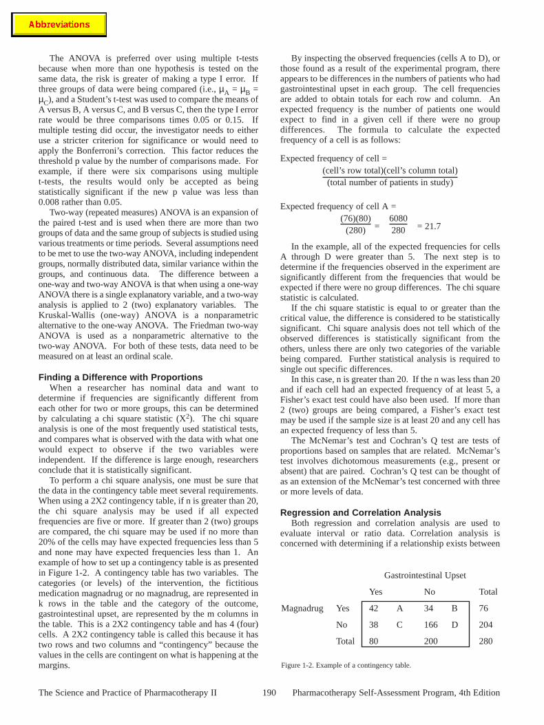
To perform a chi square analysis, one must be sure thatthe data in the contingency table meet several requirements.When using a 2X2 contingency table, if n is greater than 20,the chi square analysis may be used if all expectedfrequencies are five or more. If greater than 2 (two) groupsare compared, the chi square may be used if no more than20% of the cells may have expected frequencies less than 5and none may have expected frequencies less than 1. Anexample of how to set up a contingency table is as presentedin Figure 1-2. A contingency table has two variables. Thecategories (or levels) of the intervention, the fictitiousmedication magnadrug or no magnadrug, are represented ink rows in the table and the category of the outcome,gastrointestinal upset, are represented by the m columns inthe table. This is a 2X2 contingency table and has 4 (four)cells. A 2X2 contingency table is called this because it hastwo rows and two columns and “contingency” because thevalues in the cells are contingent on what is happening at themargins.

By inspecting the observed frequencies (cells A to D), orthose found as a result of the experimental program, thereappears to be differences in the numbers of patients who hadgastrointestinal upset in each group. The cell frequenciesare added to obtain totals for each row and column. Anexpected frequency is the number of patients one wouldexpect to find in a given cell if there were no groupdifferences. The formula to calculate the expectedfrequency of a cell is as follows:

Expected frequency of cell =

Expected frequency of cell A =

= = 21.7

In the example, all of the expected frequencies for cellsA through D were greater than 5. The next step is todetermine if the frequencies observed in the experiment aresignificantly different from the frequencies that would beexpected if there were no group differences. The chi squarestatistic is calculated.

If the chi square statistic is equal to or greater than thecritical value, the difference is considered to be statisticallysignificant. Chi square analysis does not tell which of theobserved differences is statistically significant from theothers, unless there are only two categories of the variablebeing compared. Further statistical analysis is required tosingle out specific differences.

In this case, n is greater than 20. If the n was less than 20and if each cell had an expected frequency of at least 5, aFisher’s exact test could have also been used. If more than2 (two) groups are being compared, a Fisher’s exact testmay be used if the sample size is at least 20 and any cell hasan expected frequency of less than 5.

The McNemar’s test and Cochran’s Q test are tests ofproportions based on samples that are related. McNemar’stest involves dichotomous measurements (e.g., present orabsent) that are paired. Cochran’s Q test can be thought ofas an extension of the McNemar’s test concerned with threeor more levels of data.

Regression and Correlation Analysis Both regression and correlation analysis are used to

evaluate interval or ratio data. Correlation analysis isconcerned with determining if a relationship exists between

6080280

(76)(80)(280)

(cell’s row total)(cell’s column total)(total number of patients in study)


Gastrointestinal Upset

Yes No Total

Magnadrug Yes 42 A 34 B 76

No 38 C 166 D 204

Total 80 200 280

Figure 1-2. Example of a contingency table.

191

two or more variables and describes the strength of thatrelationship. Regression on the other hand describes themagnitude of the change between the two variables. In otherwords, regression is both descriptive and predictive,whereas correlation is only descriptive.

Regression analysis provides a mathematical equationthat can be used to estimate or predict values of one variablebased on the known values of another variable. Regressionanalysis is used when there is a functional relationship thatallows investigators to predict the value of a dependent (oroutcome; y) variable from the known values of one or moreindependent (predictor; x) variable(s). When there is oneexplanatory variable, it is referred to as simple regression.When two or more explanatory variables are tested, it isreferred to as a multiple regression analysis. When theresponse variable is a binary categorical variable (e.g., deador alive), the procedure is called logistic regression.Logistic regression may be either simple or multiple logisticregression. In a study, an investigator may collect data onseveral explanatory variables, determine which variables aremore strongly associated with the response variable, andthen incorporate these variables into a regression equation.Cox proportional hazards regression is used to assess therelationship between two or more continuous or categoricalexplanatory variables and a single response variable (time tothe event). Typically, the event (e.g., death) has not yetoccurred for all participants in the sample, which createscensored observations. Elements that need to be presentedwhen describing the results of a study include the methodsfor selection of independent variables, threshold ofsignificance, and overall, how well the model worked. Inmany cases, this information is underreported.

In the case of simple linear regression, the formula forthe model is:

Dependent variable = intercept + (slope × independent variable)

The regression line is the straight line that passes throughthe data that minimizes the sum of the squared differencesbetween the original data and the line, and is referred to asthe least squares regression line. Once the linearrelationship has been determined, the next step is todetermine if there is a statistically significant relationshippresent. The coefficient of determination, r2, describes theproportion of the variation of the data presented by thedependent variable that is explained by the independentvariable. An r2 of 1.0 is a perfect relationship between thetwo variables. If the r2 value were 0.5, this is interpreted as50% of the variation in the data presented by the dependentvariable can be described by the independent variable. AnANOVA is used to determine if the differences identified aredue to chance. If a p value was found to be less than 0.05,one would conclude that there is a significant relationshipbetween the two variables of interest. The closer thecoefficient of determination is to “0”, the less likely it wouldbe to find a difference. A significant value indicates thatthere is an association, and typically not a cause and effectrelationship. This is true in most cases. An exception to thisrule is in the case of stability studies in which the

independent variable is controllable. In this case, a causeand effect relationship can be claimed.

Correlation is used to determine if two independentvariables are related in a linear manner. For instance, aninvestigator wants to determine if there is a relationshipbetween bone mineral density and the number of fractures inpostmenopausal women. A unitless number, called thecorrelation coefficient “r”, summarizes the strength of thelinear relationship between the two variables. The r valuevaries from “-1 to +1”. A “-1” indicates a perfect linearrelationship in which one variable changes while the otherchanges in an inverse fashion. The closer the calculatedvalue is to this number, the stronger the negativerelationship. A “0” indicates no relationship exists betweenthe two variables. A “+1” indicates that there is a perfectpositive linear relationship with one variable changing asthe other changes in the same direction.

Although there are several formulas used to determine thecorrelation coefficient, the most common method is thePearson’s product-moment correlation. This formula assumesnormal distribution. The Spearman correlation coefficient isthe comparable nonparametric statistic if the data are notnormally distributed. When interpreting the r value, a p valueneeds to be considered to help assess how likely thecorrelation is due to chance. If in the above example withbone mineral density and risk of fractures the relationshipbetween these two variables was determined to have an r valueof 0.97 and a p of 0.01, then the r value is significantlydifferent from 0 (no correlation) and that the finding isprobably not due to chance. If investigators conclude thatthere is a relationship between the two variables, this does notimply that there is a cause and effect relationship. Unlike theregression analysis, the correlation analysis does not describethe magnitude of the change between the two variables. Inother words, regression is both descriptive and predictive,whereas correlation is only descriptive.

Confidence Intervals A CI is the range of values consistent with the data,

which is believed to contain the actual or true mean of thepopulation. The estimate of the population mean from thesample is referred to as the point estimate. The range ofpossible means is defined as the confidence limits. The CIscan be used to estimate mean differences between groups orestimate the true mean for the population from which thesample was drawn. When considering the CI of thedifference between two groups, the 95% CI is related tostatistical significance at the 0.05 level. When the 95% CIfor the estimated difference between groups or in the samegroup over time does not include zero, the results aresignificant at the 0.05 level. For example, if the differencein mean blood pressure measurements between two groupswas 10 mm Hg (95% CI = 6–10 mm Hg), the differencebetween the groups in mean blood pressure would beconsidered to be statistically significant at the 0.05 level.Zero is not included in the area for 95% of the values overwhich the observed difference is likely to range; therefore, itmust be in the remaining 5%. The likelihood of obtaining adifference of 0 mm Hg is less than 5 times in 100.


In contrast, the mean difference in blood pressuremeasurement between two groups was 2 mm Hg(-1–5 mm Hg). Here, the CI includes zero, so the differenceis not statistically significant at the 0.05 level. Thelikelihood of obtaining a difference of 0 mm Hg is greaterthan 5 times in 100. The CI can be used as an alternative toconventional statistical tests of significance in hypothesistesting, and is most often preferred because of theinformation that can be obtained from these values. Thewidth of the CI is an indicator of the precision of theestimate; the level of significance is an indicator of theaccuracy. For a given level of confidence, the narrower theCI, the greater the precision of the sample mean as anestimate of the population means. There are three factorsthat can influence the width of the CI. First, the variance ofthe sample scores on which the CI is calculated can affectthe width of the CI, with a smaller variance resulting in anarrower CI. Although efforts could be made to obtain amore homogenous sample from the population to helpdecrease the width of the CI, in general, the investigatortypically has little control over this variable. Secondly,sampling precision can also influence the size of theinterval. Because sample precision is related to the squareroot of the sample size, doubling the sample size willdecrease the width by 25%. And the last factor is the levelof confidence that is used. If an investigator wants to be99% confident that the true mean of the population isincluded in the range of values, the CI will be wider than ifthe investigator sets the level of confidence at 95%.

In addition to the CI being used to describe differencesbetween group means or mean changes within the samegroup, the CI can also be used for proportions, odds ratios,and risk ratios. Over time, the CI can also be used forproportions, odds ratio, and risk ratios. Other commonestimates that may be accompanied by a CI include survivalrates, slopes of regression lines, effort to yield measures,and coefficients in a statistical model. The CI can also beused for a single clinical trial, but are also routinely used todescribe aggregate data in a meta-analysis.

Measures of Associationwith Categorical Data

Relative risk and odds ratio are two measures of diseasefrequency. The relative risk is the ratio of the incidence rateof an outcome in the exposed group to the incidence rate ofthe outcome in the unexposed group. The incidence rate ofa disease is a measurement of how frequently the diseaseoccurs. It is the number of new cases of the disease (in adefined time period) divided by the number of individuals inthat population at risk.

If the relative risk is 1, the risk of unintended drug effectfor an exposed person is the same as the risk for thenonexposed person. If the relative risk is greater than 1, therisk of unintended drug effect for an exposed person is Xtimes greater than that for a nonexposed person. If therelative risk is less than 1, the risk of unintended drug effectfor an exposed person is X times less than that of anonexposed person. Frequently, we would like to not only

give an indication of risk or benefit in relative terms, but onewould like to examine the actual risk. One way to describethis is by presenting the attributable risk. Attributable riskis defined as follows:

Attributable risk = incidence of gastrointestinal disease in exposed group –incidence of gastrointestinal disease in unexposed group

Another important method to describe risk is as an oddsratio. The odds ratio is an estimate of the relative risk whenthe disease under study is relatively rare. When using theodds ratio as an estimator of risk, one must assume that thecontrol group is representative of the general population, thecases are representative of the populations with the disease,and the frequency of the disease in the population is small.The odds ratio is mathematically obtained by multiplying thenumber of cases with the disease and exposed to the factorby the number of cases without the disease and not exposedto the factor and dividing this number by the number of caseswith the disease without exposure to the factor multiplied bythose cases without the disease but exposed to the factor. It isdefined by the following equation:

odds of exposure for cases A/CRelative odds =

odds of exposure for controls B/D

The odds ratio of 1 is interpreted as the number of casesthat are just as likely to have been exposed as the controls.An odds ratio of greater than 1 is interpreted as the numberof cases that are X times more likely to have been exposedthan are the controls. An odds ratio of less than 1 isinterpreted as the number of cases that are X times lesslikely to have been exposed than the control.

Confidence intervals are frequently used as a measure oftesting the significance. When a 95% CI contains 1, there isno difference between exposed and nonexposed groups.

A more detailed description of statistics commonly usedwith the pharmacoepidemiology literature is described inthe Pharmacoepidemiology chapter.

Survival Analysis Data in clinical trials may be presented using survival

curves with time-to-the-event as the dependent variable.The event or outcome may be treatment response. Patientsare followed until either they experience a predefined eventor follow-up is terminated without an end point event. Twocommon ways to calculate a life table are the actuarialapproach and the Kaplan-Meier approach. There are severalassumptions that need to be met in order to use this analysis.There needs to be an identifiable starting point. With the useof medications, the identifiable starting point is immediatelyafter the medication is given. There needs to be awell-defined outcome that is dichotomous, such as death orhospitalization. The Kaplan-Meier approach should not beused if any patients are lost to follow-up because this eventmay be related to the outcome of interest. Under thesecircumstances, the survival function will be biased with an


193

underestimation of the risk of death. Lastly, there should notbe significant differences in how patients are handled.Secular changes are changes (diagnostic practices andtreatment regimens) that occur over time, and as such,patients who were enrolled in the trial early may differ fromthose who were enrolled later. The investigator, under thesecircumstances, could not assume that he or she is dealingwith a homogeneous group, and therefore, the data shouldnot be combined.

The log-rank statistic is commonly used to compare twosurvival distributions. This test compares the observednumber of events with the numbers expected. This testworks under the assumption that if there is no differencebetween the groups, then at any interval the total number ofevents should be divided between the groups approximatelyto the number of subjects at risk. A log rank test assignsscores to each uncensored and censored observation basedon the logarithm for the estimated probability at eachobservation. If two curves are being compared and there arean equal number of patients in both groups, then each groupshould have about the same number of events.

Another test commonly used to assess survival curves isthe Cox proportional hazards model. This test has beencompared to the analysis of covariance for handling survivaldata in that it can handle any number of covariates in theequation quantifying the effect of covariates on the survivaltime. The Cox proportional hazards model is used when theresearcher is concerned about group differences at baselineand related to a covariate that is measured on a continuousscale. This allows the investigator to evaluate survival dataand adjust for confounding variables such as severity ofdisease or age.

Meta-Analysis Meta-analysis is a discipline that provides methods for

finding, appraising, and combining data from a range ofstudies to answer important questions in ways not possiblewith the results of individual studies. Meta-analysis can beused if 1) definitive clinical trials are impossible, unethical,or impractical, 2) randomized trials have been performed,but the results are conflicting, 3) results from definitivetrials are being awaited, 4) new questions not posed at thebeginning of the trial need to be answered, and 5) samplesizes are too small. From a logistical standpoint, a writtenprotocol needs to be strictly followed consistent with a goodresearch design, including a clearly defined researchquestion, search strategy, abstraction of data, and statisticalanalysis. Data are typically inspected using an L’Abbe plot.This technique is used to inspect data for heterogeneity. Theoutcome rates in treatment and control groups are plotted onthe vertical and horizontal axes. The graphical displayreveals heterogeneity of both size and direction of effect,and indicates which studies contribute most to it.

Pooling refers to methods of combining the results ofdifferent studies. This is not simply combining the datafrom all trials into one very large trial, but rather statisticallycombining results in a systematic way. Pooling mustmaintain the integrity of individual studies. In general, thecontribution of each study to the overall result is determined

by its study weight, usually the reciprocal of its variance.Details regarding the statistical methods for pooling arebeyond the scope of this chapter.

Summary A basic understanding of statistical concepts and

application is important when assessing data as thefoundation of the clinical decision-making processregarding the use of medications in patients. This chapterprovides a general overview of statistical concepts includingboth descriptive and inferential statistics. One of the morecommon mistakes made by readers of the scientificliterature is the failure to distinguish between the clinicaland statistical significance of the data. In general, data thatare clinically significant are relevant to patient care. Whenclaiming that data are statistically different, this refers to amathematical term to express a conclusion that there isevidence against the null hypothesis. The probability is lowof getting a result as extreme or more extreme than the oneobserved in the data if the null hypothesis is accepted.Merely achieving statistical significance does notcharacterize the author’s data as clinically important.Having a sound understanding of statistical concepts allowsreaders to make good judgments regarding the validity andreliability of the data, and to assess the value of the data toan individual patient or patient group. Readers are referredto the Annotated Bibliography for more detailedinformation regarding the topics described.

Annotated Bibliography1. Campbell MJ, Gardner MJ. Calculating intervals for some

nonparametric analyses. BMJ 1988;296:1454–6.

This article reviews the methodology to calculateconfidence intervals (CIs) for some nonparametric analyses,including a population median and mean (when the criteriafor normal distribution are not met). It is a well-organizeddocument that nicely outlines these two approaches. Theauthors also describe the limitations of providing CIs withnonparametric analysis. It is not always possible to calculateCIs with exactly the same level of confidence. The authorsrecommend that the 95% CI be routinely calculated. Thepaper is concisely written, easy to read, and provides somenice examples to reinforce concepts.

2. Fitzgerald SM, Flinn S. Evaluating research studies using theanalysis of variance (ANOVA): issues and interpretation.J Hand Ther 2000;13:56–60.

This article provides a critical evaluation of the singlefactor analysis of variance (ANOVA) test by providing aquestion and answer format addressing the issues that arepertinent to the evaluation of a test in a clinical trial. Itdescribes whether the ANOVA is appropriate to use, discussesits interpretation, use of post hoc test of analysis, examinationof error, and clinical interpretation. The authors do notdiscuss which post hoc test is best based for a particular dataset, but rather they provide a general review of importantconcepts to consider. The authors discuss the elements thataffect type I and type II error, including all elements thataffect power of a study.


3. Fleming TR, Lin DY. Survival analysis in clinical trials: pastdevelopments and future directions. Biometrics2000;56:971–83.

This article is a nice review of standard statisticalprocedures for assessing survival in clinical trials. The articlediscusses the more conventional methods such asKaplan-Meier approach to estimating the survival function,the log-rank statistic for comparing two survival curves, andproportional hazards model for quantifying the effects ofcovariants on survival time. The authors provide an overviewof the direction anticipated for future research activities. Thistype of analysis has gained a significant popularity in this eraof outcome management, with the science of survival analysischanging and evolving in several directions. For example, theauthors discuss the concept of integrating a Bayesianapproach in survival analysis, especially in the areas ofnoncompliance and multivariate failure time.

4. Freedman KB, Bernstein J. Sample size and statistical powerin clinical orthopaedic research. J Bone Joint Surg1999;81:1454–60.

This paper provides a nice overview of the relationshipbetween sample size and statistical power. The authorsdiscuss the concept of hypothesis testing and using a prioriselection of both types I and type II error rates. Theimplications of not having enough power relating to theinability to find a difference when a difference truly exists arenicely described. The authors also nicely describe therelationship between the elements that affect power, includingan extensive discussion on effect size, variance, error rate, andthe role of sample size. The authors also reinforce the need todo a post hoc analysis of power after completion of the study.

5. Freiman JA, Chalmers TC, Smith H, Kuebler RR. Theimportance of beta, the type II error and sample size in thedesign and interpretation of the randomized control trial.N Engl J Med 1978;299:690–4.

This article describes an analysis where the authorsreviewed 71 trials in which the investigators did not find adifference among the patient groups. The authors wereinterested in assessing the frequency by which these 71 trialslacked sufficient sample size to find a difference if one mayhave actually existed. Sixty-seven of the trials had a greaterthan 10% risk of missing a 25% difference between thegroups, and 50 of the trials missed a 50% improvement.These authors describe the implications of low power andreinforce the occurrence of this problem in the literature withthe results of their analysis.

6. Gardner MJ, Altman DG. Confidence intervals rather thanp values: estimation rather than hypothesis testing. Br Med J1986;292:746–50.

This paper provides a nice review of CIs and compares theirvalue to conventional hypothesis testing. It also describes howto calculate CIs for means and proportions. Simple andpractical examples are provided to reinforce the concepts. Thepaper also describes how CIs should be presented in theliterature, including suggestions for graphical display.

7. Greenfield ML, Kuhn JE, Wojtys EM. A statistical primer.Correlation and regression analysis. Am J Sports Med1998;26:338–43.

This review provides a nice overview of correlation andregression analysis. The information is an overview forindividuals who are unfamiliar with the concepts,

interpretation, and presentation of information. The authorsalso provide some examples throughout the document tohighlight and reinforce basic concepts. The authors reinforcethe differences between the two analyses and emphasize areasthat are commonly confused between the two functions. Toemphasize the value of regression analysis, they discuss onlythe concept of simple linear regression. This paper does notdiscuss differences with other regression analyses such asmultiple regression or logistic regression. Readers arereferred to other publications for these discussions.

8. Guyatt G, Walker S, Shannon H, Cook D, Jaeschke R, Heddle N.Correlation and regression. CMAJ 1995;152:497–504.

This article provides a nice overview of correlation andregression. With the increasing emphasis on outcome studiesusing large databases, using these statistical tests willcontinue to increase. This article is a nice primer of whenthese tests are used and how to interpret the data. The authorsuse several real examples to help describe and differentiatethese concepts. Sets of data are provided that help readers useand interpret the information. The difficulty with this articleis that the authors assume that readers have a basicunderstanding of concepts, including calculation of values.

9. Guyatt G, Jaeschke R, Heddle N, Cook D, Shannon H,Walter S. Hypothesis testing. CMAJ 1995;152:27–32.

This article provides a nice review of the statisticalconcepts of hypothesis testing and p values. The role ofchance and its relationship to probability and p value arediscussed. Simple examples, such as the toss of the coin, helpexplain these concepts to clearly reinforce the basic concepts.The authors discuss in brief the concept of type II error, typeI error related to the multiple testing problem, and limitationsof hypothesis testing. The concept of successfulrandomization and the potential need to adjust baseline valuesto improve the validity of the results also are discussed. Thisarticle reviews the basics of hypothesis testing and describescore concepts relating to the testing process.

10. Hartzema AG. Guide to interpreting and evaluating thepharmacoepidemiologic literature. Ann Pharmacother1992;26:96–7.

The article provides an overview of criteria for evaluatingthe pharmacoepidemiologic literature. The author discussesthe elements needed to evaluate research design, including thecase-control and cohort studies. He discusses how data can beinterpreted, including the use of the odds ratio, relative risk,measures of association (p value), and CIs. This is not acomplete review, but rather a simple, concise article thataddresses what a reader of pharmacoepidemiologic literaturemay need to consider in interpretation. The author does notprovide calculations or common errors in their use orinterpretation. This would not be a good article for anindividual well versed in basic concepts, but rather someonewho is new to pharmacoepidemiologic concepts.

11. Henry DA, Wilson A. Meta-analysis. Part 1. An assessment ofits aims, validity and reliability. Med J Aust 1992;156:31–8.

This review is part one of a two-part series that addresses theissue of meta-analysis, including the purpose, controversies,and the reliability and validity of the technique. This article isbasic in its approach, yet it addresses many issues pertinent toreview of the data produced by this technique. The authorsdescribe the literature that addresses the reliability and validityof meta-analysis. The authors provide a balanced review, and


195

use data to reinforce some of the areas of controversy or valueof combining data. The article also reinforces the need toprovide a systematic approach to performing a meta-analysis,as the results that are obtained can be misleading without alogical and statistically sound approach.

12. Khan KS, Chien PW, Dwarakanath LS. Logistic regressionmodels in obstetrics and gynecology literature. ObstetGynecol 1999;93:1014–20.

This study examines the variations in quality of the reportingof logistic regression in the scientific literature. Criteria weredescribed and used to assess the accuracy, precision, andinterpretation of logistic regression in 193 articles from fourgeneric obstetrics and gynecology journals in 1985, 1990, and1995. The authors found that the proportion of articles thatused logistic regression increased over this time period. Therewere several violations in quality and presentation, includingthe lack of clear reporting of dependent and independentvariables (32.1%), the selection of variables being inadequatelydescribed (51.8%), and 85.1% did not report assessment ofconformity to linear gradient. This article is a nice review forhow logistic regression should be presented in the literature. Italso reinforces the need to critically evaluate its presentationbecause of the misinformation that is frequently described.

13. Kuhn JE, Greenfield ML, Wojtys EM. A statistics primer.Hypothesis testing. Am J Sports Med 1996;24:702–3.

This article focuses on the concept of hypothesis testingand compares and contrasts the null and research hypothesis.The authors reinforce the need to clearly state the hypothesiswithin a publication, and for the reader of such an article toidentify the elements important to these concepts. Thereaders should identify the research and null hypothesis of thearticle that they are reviewing, and the meaning of the type Iand type II error of a trial. This is an important article thataddresses the development of the null hypothesis andappropriate selection of statistical analysis.

14. Lachin JM. Introduction to sample size determination andpower analysis for clinical trials. Control Clin Trials1981;2:93–113.

This article summarizes sample size determination and itsrelationship to power when planning a research project.Frequently, articles will review only one or two testingprocedures. The advantage of this article is that the authorsdiscuss methods for sample size determination for the t-test,tests for proportions, tests for survival time, and tests forcorrelations. For each example, sample values are given andcalculated. There is also a detailed discussion of power andthe elements that affect power. The article is written in aconcise, practical, and easy-to-read manner.

15. Lee ET, Go OT. Survival analysis in public health research.Annu Rev Public Health 1997;18:105–34.

Common statistical techniques for assessing survival data inpublic health research are reviewed. The authors discuss bothnonparametric and semi-parametric approaches, including theKaplan-Meier Product Limit Method, methods of testing theequality of survival distributions, and Cox’s regression model.The authors also discuss parametric models that are commonlyused, such as the accelerated failure time model. Hazardfunctions for the exponential, Weibull, gamma, Gompertz,lognormal, and log-logistic distributions are described.Examples from the literature help reinforce principles. Thereis a nice overview of commercially available software

packages that can help perform these analyses, including SAS,BMDP, SPLUS, SPSS, EGRET, and GLIM. The first two arediscussed more extensively than the others in this article.

16. Levine MA. A guide for assessing pharmacoepidemiologicstudies. Pharmacotherapy 1992;12:232–7.

The article is organized into eight primary questionsthat need to be considered when reviewing thepharmacoepidemiology literature, such as elements of studydesign, association, temporal relationship, evaluation of adose-response relationship, and other practical points relatingboth to the logistics, as well as interpretation of the data. Theauthors address many of the basic elements in evaluating thistype of literature, but that would be considered to be too basicfor a researcher in the area. This area is frequentlyoverlooked in published reviews or general tests on statistics.For more extensive, detailed information, the reader isreferred to other publications from this author and others.

17. Loney PL, Chambers LW, Bennett KJ, Roberts JG, StratfordPW. Critical appraisal of the health research literature:prevalence of incidence of a health problem. Chronic Dis Can1998;19:170–6.

This article provides an overview of how to evaluate anarticle that estimates the prevalence or incidence of a diseaseor health problem. These two terms are different, butterminology is frequently misused in the literature. Thisarticle is a primer for health professionals who have aninterest in either performing this type of research or whoreview these publications to make changes in their practice.The concepts of design, sampling frame, sample size,outcome measures, measurements, and response rates arediscussed. Examples are provided that help reinforce howdata need to be presented, interpreted, and applied to practice.

18. Mathew A, Pandey M, Murthy NS. Survival analysis: caveatsand pitfalls. Eur J Surg Oncol 1999;25:321–9.

This article discusses the concept of survival analysis, itspurpose, and appropriate use. It also discusses many methodsused to estimate the survival rate and its standard error. Theauthors discuss the concept of misusing these types of testsand guide the reader on how to properly consider issues withdata. The authors make some general recommendations,including the support of the Kaplan-Meier approach,suggesting that the median (instead of the mean) survival timebe provided whenever possible, and those confidence limitsbe used as a measure of variability. The information that isshared is practical and frequently overlooked by theinvestigators publishing studies that use survival analyses.

19. Pathic DS, Meinhold JM, Fisher DJ. Research design:sampling techniques. Am J Hosp Pharm 1980;37:998–1005.

Several statistical procedures require that one have a basicunderstanding of what constitutes a population versus asample, and whether a trial used appropriate randomizationtechniques. This article describes different types of samplingprocedures, including nonprobability samples such asconvenience samples, judgment samples, and quota sampling,and compares them to probability samples such as simplerandom sampling, stratified samples, and cluster samples.The required formulas and examples for how to calculatesample size for both estimating the population mean andestablishing population proportions are provided. Overall, itis a concise, easy-to-read article that addresses a topic that isso frequently a source of error in clinical trials.


20. Perneger TV. What’s wrong with Bonferroni adjustments.BMJ 1998;316:1236–8.

This article nicely describes the concept of multiple testingand the increased risk of type I error. Although textbooksfrequently describe this issue, they also describe usingBonferroni adjustments to resolve some of these problems.This article discusses the mechanism to adjust for multipletesting and describes the problems with this technique,including testing irrelevant null hypothesis, the increased riskof type II error, and difficulties with interpretation. Theauthors also discuss circumstances when the Bonferroniadjustment may be implemented, although they suggest thatfew situations actually exist. This is a nice document to havein your files when reviewing the concept of multiple testing.

21. Porter AM. Misuse of correlation and regression in threemedical journals. J R Soc Med 1999;92:123–8.

This review discusses some commonly found errorsrelating to the use, presentation, and interpretation of bothcorrelation and regression tests, which are frequently used inthe published literature. Several clinical trials found in theBritish Medical Journal, the New England Journal ofMedicine, and The Lancet were used. The authors identified15 different errors in the publication process: eight wereconsidered to be common. This paper is important forindividuals who are either using regression or correlation inclinical research, or for individuals who are routinelyintegrating these types of papers into their clinical practice.

22. Rigby AS. Statistical methods in epidemiology: statisticalerrors in hypothesis testing. Disabil Rehabil 1998;20:121–6.

This article on hypothesis testing describes the concept ofstatistical testing and the need to provide a systematicapproach to testing a hypothesis. The authors discuss in detailthe concept of type I and type II error, and the implications oftheir occurrence. The problem of multiple testing and itsrelationship to type I error are discussed. The concept of one-and two-tailed tests are discussed, and how p values should bepresented in the literature and what they mean. The authorsalso introduce the concept of using CIs and briefly describethe value of their use.

23. Sacks HS, Berrier J, Reitman D, Ancona-Berk VA,Chalmers TC. Meta-analyses of randomized controlled trials.N Engl J Med 1987;316:450–5.

This study provides an overview of elements that should beroutinely included in a meta-analysis. The authors reviewed86 meta-analyses in the published literature and assessed eachrelated to six major areas: study design, combinability,control of bias, statistical analysis, sensitivity analysis, andapplication of results. Only 28% of the papers reviewedaddressed all six areas. In the six major areas, a total of 23separate items were examined. Of the reviewed articles, up to14 items were satisfactorily addressed in any of the studies.This analysis of the literature reinforces the need to educateresearchers on the appropriate planning, implementing, andpresenting meta-analyses in the literature.

24. Sim J, Reid N. Statistical inference by CIs: issues ofinterpretation and utilization. Phys Ther 1999;79:186–95.

This article provides a nice review of the value of CIs,including their advantages over conventional hypothesistesting. There is a well-organized section on basic principles,interpretation, and calculation. The authors describe twobasic advantages to using CIs: 1) to attach a measure of

accuracy to a sample statistic, and 2) to interpret the questionsof clinical importance of the data. The role of CIs inmeta-analysis is also described. The authors stronglyreinforce the need to include a CI (in addition to the results ofhypothesis tests) with the level of statistical inferenceconsistent with the level of statistical significance for thehypothesis test (95% CI for p<0.05).

25. Wilson A, Henry DA. Meta-analysis. Part 2: assessing thequality of published meta-analysis. Med J Aust1992;156:173–4, 177–80, 184.

This review is part two of a two-part series (part one isdescribed in Reference 11) that reviews the elements that needto be considered in a well-designed meta-analysis. The articleis organized by using 10 questions that every investigatorneeds to address. Although they do not provide detailsregarding calculations, several issues relating to statisticalpresentation, including the need to plot results, test forheterogeneity of outcome, and to calculate a summaryestimate are addressed. The authors also discuss the conceptof publication bias, with a description of a funnel plot. As thetechnique of using meta-analysis to answer importantquestions in the literature continues to grow, this article canserve as an important checklist to use when assessing thequality of the design and validity of the results.

26. Gaddis GM, Gaddis ML. Introduction to biostatistics: Part 5,statistical inference techniques for hypothesis testing withnonparametric data. Ann Emerg Med 1990;19:153–8.

This article provides several nonparametric statistical testsused when analyzing nominal and ordinal data. It is part fiveof a six-part series that discusses basic concepts of statistics.This article is written for the individual who has littlebackground in statistics. An individual with a foundation instatistics would find this article elementary. The authors havetaken an approach of presenting information to clinicians whowill primarily be in the role of evaluating the publishedliterature instead of actually performing mathematicalcalculation of a set of data. There are few mathematicalformulas or problem-solving examples in which the readerneeds to manipulate data.

27. De Muth JE. Basic Statistics and Pharmaceutical StatisticalApplications. New York: Marcel Dekker Inc., 1999:115–48.

This chapter provides a nice overview of the concept ofnormal distribution and CIs. It reviews how to determine ifthe distribution is normal and defines and describes thecentral limit theorem. It also has a nice overview of CIs andtheir application. There are practice problems at the end ofthe chapter with answers to help reinforce concepts.


Biostatistics for the Clinician197

Questions 1 and 2 pertain to the following case.In a study that compared two different medications for thetreatment of allergic rhinitis, each patient was asked to rankhis or her severity of symptoms on a scale of 0 to 4(0 = none, 1= mild, 2 = moderate, 3 = moderately severe,and 4 = severe) 2 hours after the medication was given.

1. What type of data will be obtained from thismeasurement?

A. Interval.B. Ratio.C. Nominal.D. Ordinal.

2. Which one of the following is an appropriate method ofcentral tendency and dispersion for the data that will beobtained above?

A. Mean and standard deviation.B. Median and interquartile range.C. Median and standard deviation.D. Median, no measure of dispersion is acceptable.

3. Examine the data set of eight students with the followinggrades on a possible 100-point examination: 85, 79, 30,94, 97, 35, 87, and 88. Which one of the followingmeasures of central tendency is least affected by outliers?

A. Median.B. Mean.C. Standard deviation.D. Standard error of the mean.

4. The following data are the number of seizures for fivepatients in a study: 3, 4, 4, 6, and 8. The mean is 5.Calculate the standard deviation?

A. 1.B. 2.

C. 3.D. 4.

5. In a study that compares the cholesterol-lowering effectof a new medication to standard therapy, the mean ageof 100 patients receiving the new therapy is 40 yearsold, and the standard deviation is 4 years. Assumingnormal distribution, about what percentage of patientsis expected to be between 32 and 48 years of age?

A. 20%.B. 68%.C. 95%.D. 99%.

6. Normal distribution is an important assumption to makewhen using several statistical analyses. Which one ofthe following is an indicator of normal distribution?

A. The kurtosis is 1.B. The frequency curve is skewed to the right.C. The mean, median, and mode have similar values.D. The distribution is only modestly defined by the

mean and standard deviation.

7. The mean difference in diastolic blood pressurebetween patients taking either a new or traditionalantihypertensive is 10 mm Hg (95% confidence interval= -15 mm Hg to 51 mm Hg). The difference in diastolicblood pressure was not statistically significant at the0.05 level. What number is included in the range ofvalues that allows you to make this decision?

A. 0.B. 1.C. 2.D. 20.

SELF-ASSESSMENTQUESTIONS

Pharmacotherapy Self-Assessment Program, 4th Edition

Please start newPSAP-IV answer

sheet beforecontinuing.

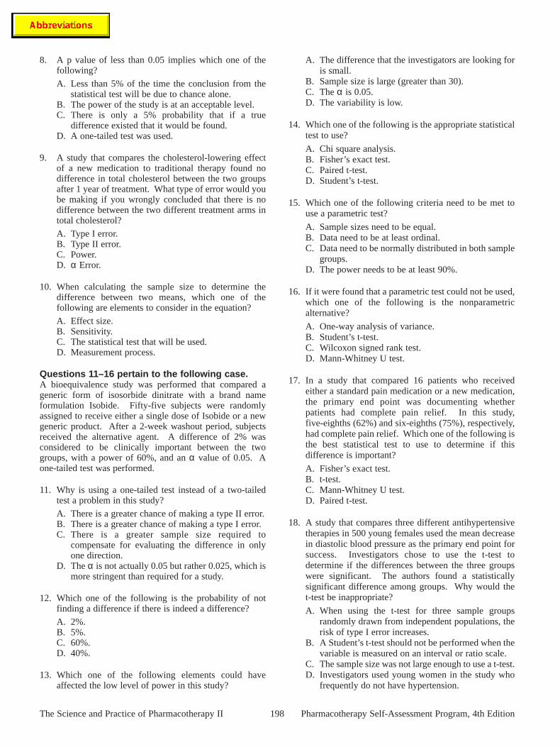
8. A p value of less than 0.05 implies which one of thefollowing?

A. Less than 5% of the time the conclusion from thestatistical test will be due to chance alone.

B. The power of the study is at an acceptable level.C. There is only a 5% probability that if a true

difference existed that it would be found.D. A one-tailed test was used.

9. A study that compares the cholesterol-lowering effectof a new medication to traditional therapy found nodifference in total cholesterol between the two groupsafter 1 year of treatment. What type of error would yoube making if you wrongly concluded that there is nodifference between the two different treatment arms intotal cholesterol?

A. Type I error.B. Type II error.C. Power.D. α Error.

10. When calculating the sample size to determine thedifference between two means, which one of thefollowing are elements to consider in the equation?

A. Effect size.B. Sensitivity.C. The statistical test that will be used.D. Measurement process.

Questions 11–16 pertain to the following case.A bioequivalence study was performed that compared ageneric form of isosorbide dinitrate with a brand nameformulation Isobide. Fifty-five subjects were randomlyassigned to receive either a single dose of Isobide or a newgeneric product. After a 2-week washout period, subjectsreceived the alternative agent. A difference of 2% wasconsidered to be clinically important between the twogroups, with a power of 60%, and an α value of 0.05. Aone-tailed test was performed.

11. Why is using a one-tailed test instead of a two-tailedtest a problem in this study?

A. There is a greater chance of making a type II error.B. There is a greater chance of making a type I error.C. There is a greater sample size required to

compensate for evaluating the difference in onlyone direction.

D. The α is not actually 0.05 but rather 0.025, which ismore stringent than required for a study.

12. Which one of the following is the probability of notfinding a difference if there is indeed a difference?

A. 2%.B. 5%.C. 60%.D. 40%.

13. Which one of the following elements could haveaffected the low level of power in this study?

A. The difference that the investigators are looking foris small.

B. Sample size is large (greater than 30).C. The α is 0.05.D. The variability is low.

14. Which one of the following is the appropriate statisticaltest to use?

A. Chi square analysis.B. Fisher’s exact test.C. Paired t-test.D. Student’s t-test.

15. Which one of the following criteria need to be met touse a parametric test?

A. Sample sizes need to be equal.B. Data need to be at least ordinal.C. Data need to be normally distributed in both sample

groups.D. The power needs to be at least 90%.

16. If it were found that a parametric test could not be used,which one of the following is the nonparametricalternative?

A. One-way analysis of variance.B. Student’s t-test.C. Wilcoxon signed rank test.D. Mann-Whitney U test.

17. In a study that compared 16 patients who receivedeither a standard pain medication or a new medication,the primary end point was documenting whetherpatients had complete pain relief. In this study,five-eighths (62%) and six-eighths (75%), respectively,had complete pain relief. Which one of the following isthe best statistical test to use to determine if thisdifference is important?

A. Fisher’s exact test.B. t-test.C. Mann-Whitney U test.D. Paired t-test.

18. A study that compares three different antihypertensivetherapies in 500 young females used the mean decreasein diastolic blood pressure as the primary end point forsuccess. Investigators chose to use the t-test todetermine if the differences between the three groupswere significant. The authors found a statisticallysignificant difference among groups. Why would thet-test be inappropriate?

A. When using the t-test for three sample groupsrandomly drawn from independent populations, therisk of type I error increases.

B. A Student’s t-test should not be performed when thevariable is measured on an interval or ratio scale.

C. The sample size was not large enough to use a t-test.D. Investigators used young women in the study who

frequently do not have hypertension.


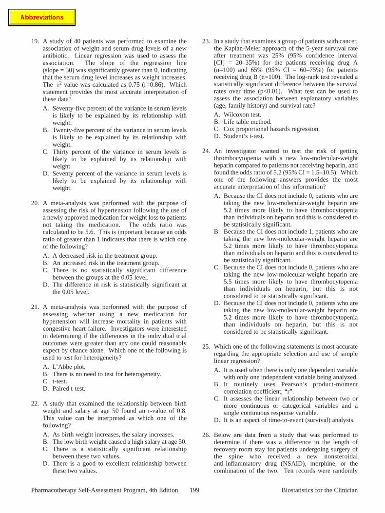
199

19. A study of 40 patients was performed to examine theassociation of weight and serum drug levels of a newantibiotic. Linear regression was used to assess theassociation. The slope of the regression line(slope = 30) was significantly greater than 0, indicatingthat the serum drug level increases as weight increases.The r2 value was calculated as 0.75 (r=0.86). Whichstatement provides the most accurate interpretation ofthese data?

A. Seventy-five percent of the variance in serum levelsis likely to be explained by its relationship withweight.

B. Twenty-five percent of the variance in serum levelsis likely to be explained by its relationship withweight.

C. Thirty percent of the variance in serum levels islikely to be explained by its relationship withweight.

D. Seventy percent of the variance in serum levels islikely to be explained by its relationship withweight.

20. A meta-analysis was performed with the purpose ofassessing the risk of hypertension following the use ofa newly approved medication for weight loss to patientsnot taking the medication. The odds ratio wascalculated to be 5.6. This is important because an oddsratio of greater than 1 indicates that there is which oneof the following?

A. A decreased risk in the treatment group.B. An increased risk in the treatment group.C. There is no statistically significant difference

between the groups at the 0.05 level.D. The difference in risk is statistically significant at

the 0.05 level.

21. A meta-analysis was performed with the purpose ofassessing whether using a new medication forhypertension will increase mortality in patients withcongestive heart failure. Investigators were interestedin determining if the differences in the individual trialoutcomes were greater than any one could reasonablyexpect by chance alone. Which one of the following isused to test for heterogeneity?

A. L’Abbe plot.B. There is no need to test for heterogeneity.C. t-test.D. Paired t-test.

22. A study that examined the relationship between birthweight and salary at age 50 found an r-value of 0.8.This value can be interpreted as which one of thefollowing?

A. As birth weight increases, the salary increases.B. The low birth weight caused a high salary at age 50.C. There is a statistically significant relationship

between these two values.D. There is a good to excellent relationship between

these two values.

23. In a study that examines a group of patients with cancer,the Kaplan-Meier approach of the 5-year survival rateafter treatment was 25% (95% confidence interval[CI] = 20–35%) for the patients receiving drug A(n=100) and 65% (95% CI = 60–75%) for patientsreceiving drug B (n=100). The log-rank test revealed astatistically significant difference between the survivalrates over time (p<0.01). What test can be used toassess the association between explanatory variables(age, family history) and survival rate?

A. Wilcoxon test. B. Life table method.C. Cox proportional hazards regression.D. Student’s t-test.

24. An investigator wanted to test the risk of gettingthrombocytopenia with a new low-molecular-weightheparin compared to patients not receiving heparin, andfound the odds ratio of 5.2 (95% CI = 1.5–10.5). Whichone of the following answers provides the mostaccurate interpretation of this information?

A. Because the CI does not include 0, patients who aretaking the new low-molecular-weight heparin are5.2 times more likely to have thrombocytopeniathan individuals on heparin and this is considered tobe statistically significant.

B. Because the CI does not include 1, patients who aretaking the new low-molecular-weight heparin are5.2 times more likely to have thrombocytopeniathan individuals on heparin and this is considered tobe statistically significant.

C. Because the CI does not include 0, patients who aretaking the new low-molecular-weight heparin are5.5 times more likely to have thrombocytopeniathan individuals on heparin, but this is notconsidered to be statistically significant.

D. Because the CI does not include 0, patients who aretaking the new low-molecular-weight heparin are5.2 times more likely to have thrombocytopeniathan individuals on heparin, but this is notconsidered to be statistically significant.

25. Which one of the following statements is most accurateregarding the appropriate selection and use of simplelinear regression?

A. It is used when there is only one dependent variablewith only one independent variable being analyzed.

B. It routinely uses Pearson’s product-momentcorrelation coefficient, “r”.

C. It assesses the linear relationship between two ormore continuous or categorical variables and asingle continuous response variable.

D. It is an aspect of time-to-event (survival) analysis.

26. Below are data from a study that was performed todetermine if there was a difference in the length ofrecovery room stay for patients undergoing surgery ofthe spine who received a new nonsteroidalanti-inflammatory drug (NSAID), morphine, or thecombination of the two. Ten records were randomly


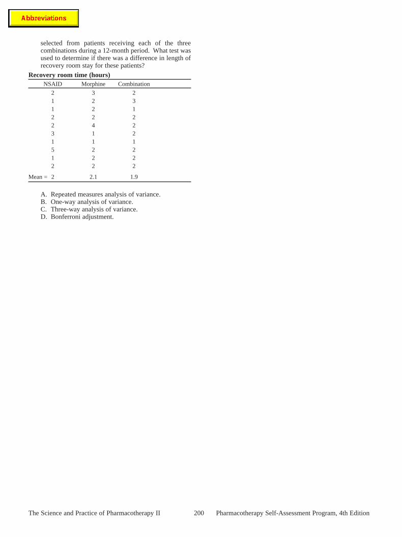
selected from patients receiving each of the threecombinations during a 12-month period. What test wasused to determine if there was a difference in length ofrecovery room stay for these patients?

Recovery room time (hours)NSAID Morphine Combination

2 3 21 2 31 2 12 2 22 4 23 1 21 1 15 2 21 2 22 2 2

Mean = 2 2.1 1.9

A. Repeated measures analysis of variance.B. One-way analysis of variance.C. Three-way analysis of variance.D. Bonferroni adjustment.


Documents

BIOSTATISTICS FOR THE CLINICIAN - Pharmaceutical · PDF file183 Biostatistics for the Clinician Learning Objectives 1. Understand when to use and how to calculate and interpret different