Biostatistics.

Summary

2

The biostatics exam

The biostatics exam will be together with the exam of Physics on the same day. The biostatistical part will be a computer aided single choice test exam during 30 minutes.

Only formula sheet can be used, it will be given.

At the biostatistic exam a maximum of 20 points can be achieved.

Exam grades: 0-9 point : failed

10-11 point: passed

12-14 point: acceptable

15-17 point: good

18-20 point: very good.

In case of a successful exam the number of points will be added to result of Physics

exam. The final mark depends on 1/3 part biostatistics and 2/3 part physics

knowledge

If either part (physics or statistics) of the exam is failed, the whole exam procedure

will have to be repeated.

Permitted use

Formula sheet will be given.

The use of simple calculators is permitted

(but you can use the calculator of the

computer). Mobile phones, tablets, etc. are

forbidden.

3

Consultations in the exam period Every thuesday in the exam period there will be consultations in

Room 25 for the students having exam within one week.

13:00-14:00: biostatistics, 14:00-15:00 physics

Check for exact dates and time on the homepage of the institut!

http://www2.szote.u-szeged.hu/dmi/

4

Types of questions 10 questions about the theory – list of all questions are

given on the homepage of the Institut

10 questions of problem-solving – list of all problem

types are given on the homepage of the Institut

Given the problem, the question might be:

find the appropriate method

find the null-and alternative hypothesis

find the critical value in the table

calculate the test statistic, i.e., t, 2, etc. (formula sheet can be used)

decide about the significance based on test statistic and the critical

value in the table

decide about significance based on p-value

Calculations (descriptive statistics, simple probabilities, confidence

interval, test statistic( t, 2)): 4-5-6 of 10 questions

Finding the method, null-and alternative hypotheses, finding critical

values, decision: 4-5-6 of the 10 questions5

Teaching files

To be download (lecture files, formula sheet,

type of questions and problems, manuscript):

Homepage of the Institut http://www2.szote.u-

szeged.hu/dmi/eng/

Coospace, Medical Physics and Statistics 1st

lecture

Recommended literature http://davidmlane.com/hyperstat/index.html

http://ebookee.org/Primer-of-Biostatistics_148268.html

6

7

Summary of the topics

Descriptive statistics

Hypothesis tests

8

Descriptive statistics

Categorical Continuous

Characterising data (variables)

Distribution, distribution function Density function, distribution function

Frequencies, relative frequencies Histogram, cumulative histogram

Sample characteristics:

Central: mean, median, mode

Dispersion: min-max, percentiles, quartiles,

Standard deviation

Special distributions

Binomial (n.p) Uniform

Poisson(np=) Normal ->properties!!

Uniform (t, F, 2 distribution)

Central limit theorem, standard error of mean

Estimations: statistic, confidence interval

Confidence interval for the mean of a normal

distribution in case of known and unknown

standard deviation

9

Calculation of the mean, median and standard deviation of (a few) given numbers

Given the following of the following small sample: X: 4 ; 1 ; 5 ; 4 ; 1 , calculate mean, median, mode, range, standard deviation!

Mean=(4+1+5+4+1)/5=15/5=3

Median. First order your data:

1

1

4

4

5

Range: maximum – minimum=5-1=4

Median: the element in the middle (or if there are two middle

elements, take their means)

10

Calculation of the mean, median and standard deviation of (a few) given numbers

Standard deviation.

The mean was 3. Calculate the nominator using the table:

iancen

xx

SD

n

i

i

var1

)(1

2

4 1 1

1 -2 4

5 2 4

4 1 1

1 -2 4

Total 0 14

ix xxi 2)( xxi

87.15.34

14

1

)(1

2

n

xx

SD

n

i

i

11

Hypothesis tests

Hypothesis: a statement about the

population

Based on our data (sample) we conclude

to the whole phenomenon (population)

We examine whether our result (difference

in samples) is greater then the difference

caused only by chance.

12

Steps of hypothesis-testing

Step 1-2. State the null hypothesis H0 and the motivated (alternative) hypothesis Ha.

Step 3. Select the , the probability of Type I error, or the α significance level. Most often α =0.05 or α =0.01.

Step 4. Choose the size n of the random sample

Step 5. Select a random sample from the appropriate population and obtain your data.

Step 6. Calculate the decision rule –it depends on problem, assumptions, type of data, etc... Comparison of means – t-test, ANOVA

Comparison of variances: F-test

Comparison of frequencies: khi-square test

Step 7. Decision.

a) Reject the null hypothesis, i.e., accept Ha

the difference is significant at α100% level.

b) Fail to reject the null hypothesis, accept H0

the difference is not significant at α100% level.

The appropriate test depends on the type of data, on

the experiment and on the aim of comparison

The following tests have been used in this course:

13

One variable (continuous): compared to a known value: One-Sample t-test

Two variables:

1) both are continuous (measured on the same subject):

a) comparing the means of variables (mean change) : Paired t-test (one sample t-test of

the differences)

b) examining relationships between variables: correlation, regression

2) one continuous dependent variable divided into unrelated groups according to another,

categorical variable: (that is, comparing means of groups)

a) number of groups=2: two-sample t-test (Independent t-test)

b) number of groups>2: One-way ANOVA (Analysis of Variance)

3) both are categorical: examination of contingency tables, chi-square test

In 1) and 2) we assumed that the samples come from normal distribution. If this assumption

does not hold or we have ordered data, use nonparametric methods based on ranks.

14

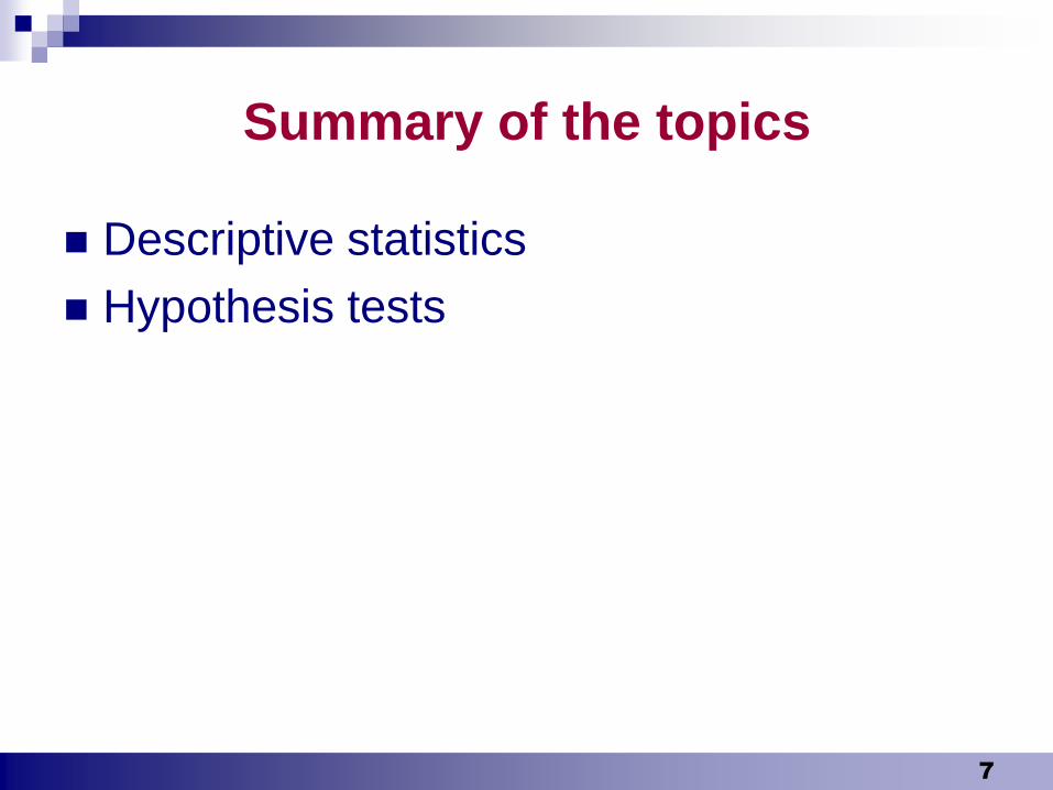
Finding significance, paired t-test There are two related data (typically

before and after a treatment).

H0: diff=0. The null hypothesis states that there is no change in the population, the mean difference is 0.

We can calculate the t-value (test statistic) according to the formula

If the null hypothesis is true, we know the distribution of the calculated t-value : it is a t-distribution with n-1 degrees of freedom. So the calculated t-value lies in the acceptance area with high (1-) probability, given by the critical values in the table.

y=student(x;49)

-3 -2 -1 0 1 2 3

0.0

0.1

0.2

0.3

0.4

0.5

p=2*(1-istudent(abs(x);49))

-3 -2 -1 0 1 2 3

0.0

0.2

0.4

0.6

0.8

1.0

dSE

dt

Acceptance area

ttable-ttable

15

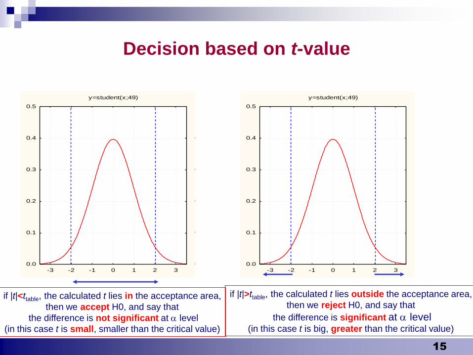
Decision based on t-value

y=student(x;49)

-3 -2 -1 0 1 2 3

0.0

0.1

0.2

0.3

0.4

0.5

p=2*(1-istudent(abs(x);49))

-3 -2 -1 0 1 2 3

0.0

0.2

0.4

0.6

0.8

1.0

y=student(x;49)

-3 -2 -1 0 1 2 3

0.0

0.1

0.2

0.3

0.4

0.5

p=2*(1-istudent(abs(x);49))

-3 -2 -1 0 1 2 3

0.0

0.2

0.4

0.6

0.8

1.0

if |t|<ttable, the calculated t lies in the acceptance area,

then we accept H0, and say that

the difference is not significant at level

(in this case t is small, smaller than the critical value)

if |t|>ttable, the calculated t lies outside the acceptance area,

then we reject H0, and say that

the difference is significant at level(in this case t is big, greater than the critical value)

16

Decision based on p-value

p-value: the tail areas under the density curve of H0 cut by the calculated t-value (The probability of the observed test statistic as is or more extreme in either direction when the null hypothesis is true).

p<, the difference is significant at levelp>, the difference is not significant at level

17

Finding significance

Based on test statistic (t-value, F-value, 2 value) – you need a critical value in the statistical table according to and degrees of freedom.

If |t|<ttable, the difference is not

significant at level

Do not reject H0 (accept H0)

If |t|>ttable, the difference is significant at

level

Reject H0 (accept HA)

Based on p-value, you simply compare p-value and (you do not need critical values).

If p> the difference is not

significant at level

Do not reject H0 (accept H0)

If p<, the difference is significant

at level

Reject H0 (accept HA)

18

Paired t-test, example

A study was conducted to determine weight loss, body composition, etc. in obese women before and after 12 weeks of treatment with a very-low-calorie diet .

We wish to know if these data provide sufficient evidence to allow us to conclude that the treatment is effective in causing weight reduction in obese women.

The mean difference is actually 4. Is it a real difference? Big or small? If the study were to be repeated, would we get the same result or less, even 0?

Before After Difference

85 86 -1

95 90 5

75 72 3

110 100 10

81 75 6

92 88 4

83 83 0

94 93 1

88 82 6

105 99 6

Mean 90.8 86.8 4.

SD 10.79 9.25 3.333

19

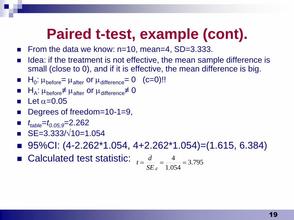
Paired t-test, example (cont). From the data we know: n=10, mean=4, SD=3.333.

Idea: if the treatment is not effective, the mean sample difference is small (close to 0), and if it is effective, the mean difference is big.

H0: before= after or difference= 0 (c=0)!!

HA: before≠ after or difference≠ 0

Let =0.05

Degrees of freedom=10-1=9,

ttable=t0.05,9=2.262

SE=3.333/10=1.054

95%CI: (4-2.262*1.054, 4+2.262*1.054)=(1.615, 6.384)

Calculated test statistic: 795.3054.1

4

dSE

dt

20

Paired t-test, example (cont.)

Decision based on confidence interval:

95%CI:(4-2.262*1.054, 4+2.262*1.054)=(1.615, 6.384)

If H0 is true, 0 is inside the confidence interval

Decision: now 0 is outside the confidence interval, we decide to reject H0 , the difference is significant at 5% level, the treatment was effective.

The mean loss of body weight was 4 kg, which could be even 6.36 but minimum 1.615, with 95% probability.

21

Decision based on t-value and on p-value

Decision based on test statistic (t-value):

This t has to be compared to the critical t-value in the table.

|t|=3.795>2.262(=t0.05,9), the difference is significant at 5% level

Decision based on p-value:

p=0.004, p<0.05, the difference is significant at 5% level

Acceptance region

ttable, critical value

tcomputed, test statistic

795.3054.1

4

dSE

dt

22

Statistical tests studied and their null

hypotheses

One-sample t-test

Aim: comparison of the mean to a given

constant c

Assumption: normality

H0: μ=c,the population mean =c

Ha: μc,the population mean c

Test statistic:

df=n-1SE

cxt

23

Statistical tests studied and their null

hypotheses

Paired t-test

Aim: comparison of the means of two related samples

(comparison the mean difference to 0)

Assumption: normality of the differences

H0: μ1=μ2 or μdiff =0, the population means are equal

Ha: μ1 μ2 or μdiff 0, the population means are different

Test statistic: ,

sample mean difference/SE of differences

df=n-1

dSE

dt

24

Statistical tests studied and their null

hypotheses Two-sample t-test or independent sample t-test

Aim: comparison of the means of two independent samples

Assumption: both samples are drawn from a normal distribution and their variances are equal

H0: μ1=μ2 or μdiff =0, the population means are equal

Ha: μ1 μ2 or μdiff 0, the population means are different

Test statistic, in case of equal variances

df=n+m-2

Test statistic, in case of unequal variances (Welch test)

df =

mn

nm

SD

yx

mnSD

yxt

pp

11

m

SD

n

SD

yxd

yx

22

( ) ( )

( ) ( ) ( )

n m

g m g n

1 1

1 1 12 2

m

SD

n

SD

n

SD

gyx

x

22

2

2

)1()1( 22

2

mn

SDmSDnSD

yx

p

25

Statistical tests studied and their null

hypotheses F-test

Aim: comparison of the variances of two independent samples

Assumption: both samples are drawn from a normal distribution

H0: 12 = 2

2 , the population variances are equal

HA: 12 < 2

2 or 12 > 2

2, the population variances are different (one-

sided alternative)

Test statistic

Degrees of freedom 1. Sample size of the nominator-1

2. Sample size of the denominator-1

variancesamplesmalle

variancesamplehigher

),min(

),max(22

22

yx

yx

SDSD

SDSDF

26

Statistical tests studied and their null

hypotheses

One-way ANOVA

Aim: comparison of the means of several independent samples

Assumption: all samples are drawn from a normal distribution and their variances are equal

H0: μ1=μ2 = …= μt, the population means are equal

HA: there is at least one mean different from another

Test statistic comes from the ANOVA table (F-value)

df: h-1, N-h

Source of variation Sum of squares Degrees of freedom Variance F

Between groups Q n x xb

i

h

i i

1

2( )

h-1 sQ

hb

b2

1

F

s

s

b

w

2

2

Within groups Q x xw

i

h

j

n

ij i

i

1 1

2( )

N-h sQ

N hw

w2

Total Q x xi

h

j

n

ij

i

1 1

2( )

N-1

27

Statistical tests studied and their null

hypotheses

Chi-square-test for independence

Aim: comparison of the distributions of categorical

variables

Assumption: big sample size expressed in expected

frequencies: expected frequencies <5 in max. 20% cell

H0: independence, the two variables are independent

Ha: the two variables are dependent

Test statistic:

df=(number of columns-1)(number of rows-1)

i

ii

E

EOX

22 )(

28

Statistical tests studied and their null

hypotheses Nonparametric tests based on ranks

Aim: comparison of samples, where normality does not

hold or when data are measured on ordinal scale

Assumption: continuous distribution

H0: the samples are drawn from the same population

Ha: the samples are drawn from the different

populations

Test statistic: sum of ranks

Decision:

tables (small simple size)

Z-value ~N(0,1) (large sampe size)

Exact p-value (software)

29

Statistical tests studied and their null

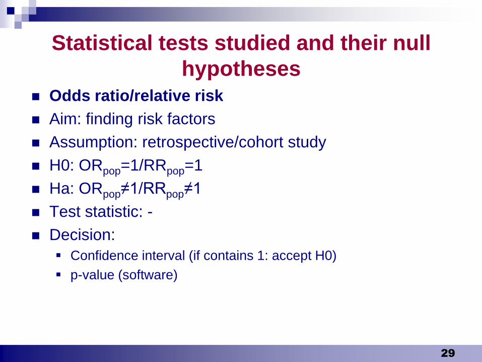
hypotheses Odds ratio/relative risk

Aim: finding risk factors

Assumption: retrospective/cohort study

H0: ORpop=1/RRpop=1

Ha: ORpop≠1/RRpop≠1

Test statistic: -

Decision:

Confidence interval (if contains 1: accept H0)

p-value (software)

30

Statistical tests studied and their null

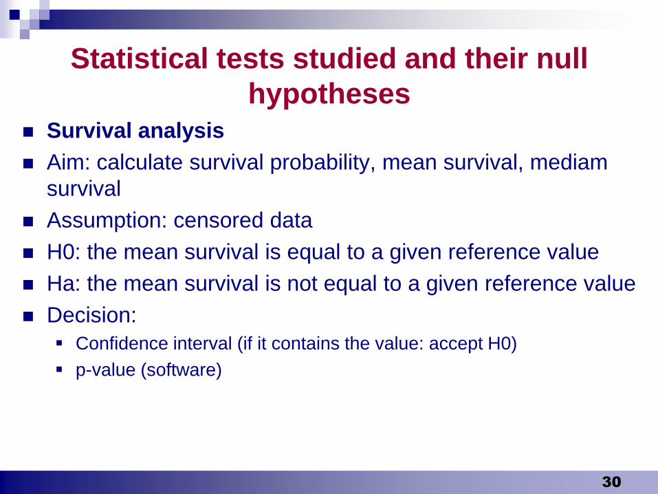
hypotheses Survival analysis

Aim: calculate survival probability, mean survival, mediam

survival

Assumption: censored data

H0: the mean survival is equal to a given reference value

Ha: the mean survival is not equal to a given reference value

Decision:

Confidence interval (if it contains the value: accept H0)

p-value (software)

Examples from the medical literature

31

Baseline demographic and clinical characteristicsWhat kind of test were used to get the given p-values? What is their meaning?

32

Baseline demographic and clinical characteristicsWhat kind of test were used to get the given p-values? What is their meaning?

33

Two-sample t-test

Chi-squared test

Baseline demographic and clinical characteristicsWhat kind of test were used to get the given p-values? What is their meaning?

34

The only statistically significant difference at 5% level is the difference between mean weights

Orvosi Hetilap

35

36

37

38

39

40

Medical use of statistics

During your study at the university, you will find

statistics in the medical subjects

Thesis

During your life you will find statistics in

Research

Medical papers

In pharmaceutical industry

…..

41

So

don’t forget statistics!