University of Nebraska - LincolnDigitalCommons@University of Nebraska - Lincoln

Other Publications in Wildlife Management Wildlife Damage Management, Internet Center for

Spring 3-9-2017

Biotic and abiotic factors predicting the globaldistribution and population density of an invasivelarge mammalJesse S. LewisConservation Science Partners, Fort Collins, CO, jslewis.research@gmail.com

Mathew L. FarnsworthConservation Science Partners, Fort Collins, CO

Christopher L. BurdettColorado State University

David M. TheobaldConservation Science Partners, Truckee, California

Miranda GrayConservation Science Partners, Truckee, CA

See next page for additional authors

Follow this and additional works at: http://digitalcommons.unl.edu/icwdmother

Part of the Agriculture Commons, Biology Commons, and the Population Biology Commons

This Article is brought to you for free and open access by the Wildlife Damage Management, Internet Center for at DigitalCommons@University ofNebraska - Lincoln. It has been accepted for inclusion in Other Publications in Wildlife Management by an authorized administrator ofDigitalCommons@University of Nebraska - Lincoln.

Lewis, Jesse S.; Farnsworth, Mathew L.; Burdett, Christopher L.; Theobald, David M.; Gray, Miranda; and Miller, Ryan S., "Biotic andabiotic factors predicting the global distribution and population density of an invasive large mammal" (2017). Other Publications inWildlife Management. 79.http://digitalcommons.unl.edu/icwdmother/79

AuthorsJesse S. Lewis, Mathew L. Farnsworth, Christopher L. Burdett, David M. Theobald, Miranda Gray, and RyanS. Miller

This article is available at DigitalCommons@University of Nebraska - Lincoln: http://digitalcommons.unl.edu/icwdmother/79

University of Nebraska - LincolnDigitalCommons@University of Nebraska - Lincoln

Other Publications in Wildlife Management Wildlife Damage Management, Internet Center for

Spring 3-9-2017

Biotic and abiotic factors predicting the globaldistribution and population density of an invasivelarge mammalJesse S. Lewis

Mathew L. Farnsworth

Christopher L. Burdett

David M. Theobald

Miranda Gray

See next page for additional authors

Follow this and additional works at: http://digitalcommons.unl.edu/icwdmother

Part of the Agriculture Commons, Biology Commons, and the Population Biology Commons

This Article is brought to you for free and open access by the Wildlife Damage Management, Internet Center for at DigitalCommons@University ofNebraska - Lincoln. It has been accepted for inclusion in Other Publications in Wildlife Management by an authorized administrator ofDigitalCommons@University of Nebraska - Lincoln.

AuthorsJesse S. Lewis, Mathew L. Farnsworth, Christopher L. Burdett, David M. Theobald, Miranda Gray, and RyanS. Miller

1Scientific RepoRts | 7:44152 | DOI: 10.1038/srep44152

www.nature.com/scientificreports

Biotic and abiotic factors predicting the global distribution and population density of an invasive large mammalJesse S. Lewis1, Matthew L. Farnsworth1, Chris L. Burdett2, David M. Theobald1, Miranda Gray3 & Ryan S. Miller4

Biotic and abiotic factors are increasingly acknowledged to synergistically shape broad-scale species distributions. However, the relative importance of biotic and abiotic factors in predicting species distributions is unclear. In particular, biotic factors, such as predation and vegetation, including those resulting from anthropogenic land-use change, are underrepresented in species distribution modeling, but could improve model predictions. Using generalized linear models and model selection techniques, we used 129 estimates of population density of wild pigs (Sus scrofa) from 5 continents to evaluate the relative importance, magnitude, and direction of biotic and abiotic factors in predicting population density of an invasive large mammal with a global distribution. Incorporating diverse biotic factors, including agriculture, vegetation cover, and large carnivore richness, into species distribution modeling substantially improved model fit and predictions. Abiotic factors, including precipitation and potential evapotranspiration, were also important predictors. The predictive map of population density revealed wide-ranging potential for an invasive large mammal to expand its distribution globally. This information can be used to proactively create conservation/management plans to control future invasions. Our study demonstrates that the ongoing paradigm shift, which recognizes that both biotic and abiotic factors shape species distributions across broad scales, can be advanced by incorporating diverse biotic factors.

Predicting and mapping species distributions, including geographic range and variability in abundance, is fun-damental to the conservation and management of biodiversity and landscapes1. The ecological niche defines species-habitat relationships2–4 and provides a useful framework for understanding the range and abundance of species in relation to biotic and abiotic factors. Further, niche relationships across local scales can provide novel information about the ecology, conservation, and management of species at macro scales5. Most studies evaluat-ing a species’ niche across their distribution focus on presence-absence occurrence data to predict the geographic range6; however, conservation and management plans for species can be improved by understanding patterns of population abundance and density across a species’ range7. In particular, evaluating population density, compared to occurrence, can reveal novel patterns of species distributions in relation to landscape factors8.

There is an ongoing paradigm shift in understanding how biotic and abiotic factors shape species distribu-tions. Until recently, it was widely accepted that abiotic factors, such as temperature and precipitation, played the primary role in shaping distributions of species and biodiversity at broad scales (e.g., regional, continental, global extents) and that biotic factors were most important at fine scales (e.g., site, local extents)9–11. It is increas-ingly recognized, however, that biotic factors are important determinants of species distributions at broad spatial scales, especially when considering biotic interactions12–16. Although interspecific competition can be an impor-tant biotic determinant in species distribution models at broad scales, other forms of biotic interactions, such as

1Conservation Science Partners, 5 Old Town Sq, Suite 205, Fort Collins, Colorado, 80524, USA. 2Colorado State University, Department of Biology, Fort Collins, Colorado, 80524, USA. 3Conservation Science Partners, 11050 Pioneer Trail, Suite 202, Truckee, California, 96161, USA. 4United States Department of Agriculture, Animal and Plant Health Inspection Service, Veterinary Services, Center for Epidemiology and Animal Health, Fort Collins, Colorado, 80524, USA. Correspondence and requests for materials should be addressed to J.S.L. (email: jslewis.research@gmail.com)

received: 04 November 2016

Accepted: 03 February 2017

Published: 09 March 2017

OPEN

www.nature.com/scientificreports/

2Scientific RepoRts | 7:44152 | DOI: 10.1038/srep44152

predation and symbioses, can also be important determinants15,17, but have received less attention18. In addition, although researchers have evaluated the effects of biotic interactions on geographic range limits18, relatively few studies have evaluated how biotic factors influence population density across a species’ range19,20, which can be more informative in understanding macro-ecological patterns7,21.

In addition to species interactions, biotic factors related to vegetation can influence species distributions and abundance at broad scales. In particular, anthropogenic land-use change is rarely considered when evaluating species distributions at broad scales; however, given the human footprint globally22 and projections for expand-ing human impacts on the environment23,24, biotic factors created by human activities are potentially important predictors that can contribute to a better understanding of species distributions8. For example, agricultural crops are a dominant biotic factor across continents that are facilitated by human engineering and the redistribution of ecological resources and energy, which can have profound impacts on plant and animal populations across broad extents; agriculture can increase populations for some species through increased food, resource availability, and landscape heterogeneity, or decrease populations due to loss of habitat25–27. Ultimately, further evaluation is nec-essary to understand the relative importance of abiotic and biotic factors in shaping species distributions across broad spatial scales13,15.

Invasive species are a primary driver of widespread and severe negative impacts to ecosystems, agriculture, and humans across local to global scales28. These introduced plants and animals often exhibit broad geographic distributions, can be relatively well studied across local scales, and provide novel opportunities to evaluate broad-scale patterns of niche relationships29. Predictions of potential geographic distribution of invasive species can provide critical information that can inform the prevention, eradication, and control of populations, which has been evaluated for many taxa, including plants30, amphibians31, and invertebrates32. However, few studies have predicted the potential ranges and abundance of non-native mammals33. Especially for wide-ranging species that can occur across broad extents of landscapes, predictions of how population density varies spatially can provide important information for prioritizing conservation and management actions.

Few species exhibit a global distribution that extends across Europe, Asia, Africa, North and South America, Australia, and oceanic Islands. Besides naturalized animals, such as the house mouse (Mus musculus) and brown rat (Rattus norvegicus), wild pigs (Sus scrofa; other common names include wild boar, wild/feral swine, wild/feral hog, and feral pig) have one of the widest geographic distributions of any mammal; further, it exhibits the widest geographic range of any large mammal34, with the exception of humans. The expansive global distribu-tion of wild pigs is attributed to its broad native range in Eurasia and northern Africa, widespread introduction by humans outside its native range, and superior adaptability, where it occurs in a wide variety of ecological communities, ranging from deserts to temperate and tropical environments35,36, with a corresponding diverse omnivorous diet37. Across its non-native range (Fig. 1; Supplementary Methods S1), including North and South America, Australia, sub-Saharan Africa, and many islands, wild pigs are considered one of the 100 most harmful invasive species in the world38 due to wide-ranging ecosystem disturbance, agricultural damage, pathogen and disease vectors to wildlife, livestock and people, and social impacts to people and property39–41. Wild pigs are therefore a model species to evaluate biotic and abiotic factors associated with population density because they exhibit a global distribution across six continents, are widely studied across much of their native and non-native (i.e., invasive or introduced) ranges, and previous research has indicated that their population density was related to abiotic factors across a continental scale, although it was ambiguous how biotic factors shape their abundance, warranting further study42.

To address these ecological questions and understand the relative importance of biotic and abiotic factors in shaping the global distribution of a highly invasive mammal, we evaluated estimates of population density of wild pigs across diverse environments on five continents. Specifically, we (1) evaluate how biotic (i.e., vegetation and

Figure 1. Geographic range of wild pigs across their native and non-native global distribution. Areas of white indicate locations in which wild pigs are likely not present. This map was created using ArcGIS 10.3.198. See Supplementary Methods S1 for a description of methods and citations used for creating the map of wild pig global distribution across its native and non-native ranges.

www.nature.com/scientificreports/

3Scientific RepoRts | 7:44152 | DOI: 10.1038/srep44152

predation) and abiotic (i.e., climate) factors (Table 1) shape population density across a global scale and (2) create a predictive distribution map of potential population density across the world. We also compare population den-sity between island and mainland populations. Our results contribute novel insight into the relative roles of biotic and abiotic factors in shaping the distribution of species’ population densities across continental and global scales, particularly relating to human-mediated land-use change, which can provide critical information to management and conservation strategies.

ResultsWe compiled 147 estimates of wild pig density (# animals/km2), which resulted in 129 estimates of density across their global distribution used in our analyses (Fig. 1; Supplementary Table S2). Some areas contained > 1 density estimate, and these were averaged. Population density of wild pigs was higher on islands (n = 11) compared to on the mainland (n = 118) (t = 4.72, df = 10.93, p < 0.001; Supplementary Figure S3). For the untransformed den-sity estimates, mean population density for on the mainland equaled 2.75 (se = 0.38) and islands equaled 18.52 (se = 4.15). The highest estimates of population density occurred on islands, which reached upwards of 40 wild pigs/km2 (Supplementary Table S2). Due to differences in population density between islands and on the main-land, we used density estimates from mainland populations in our subsequent analyses.

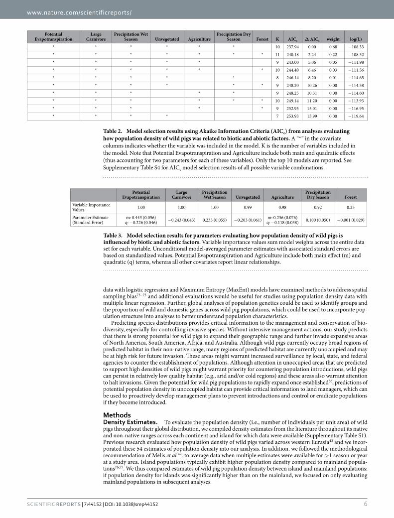
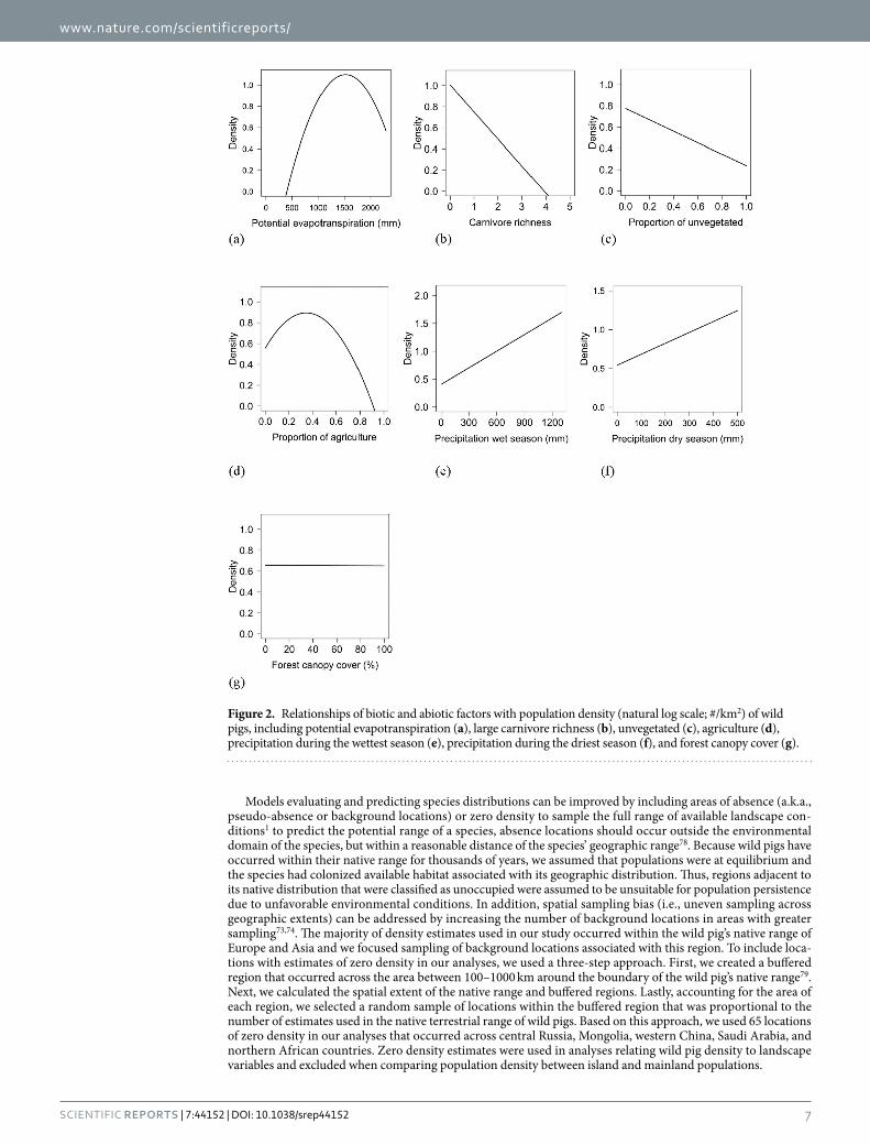
Population density was influenced by both biotic and abiotic factors across the global distribution (Tables 2 and 3; Supplementary Table S4). The suite of best models all included combinations of biotic and abiotic factors (Table 2) and the top model (AICc = 237.94; model weight = 0.68; adjusted R2 = 0.55) had > 1,000 times more support as the best approximating model than the top model considering only abiotic factors (AICc = 311.30; model weight = 7.94 × 10−17) (Supplementary Table S4). The variables with the greatest importance included potential evapotranspiration, large carnivore richness, precipitation during the wet and dry seasons, unvege-tated area, and agriculture, which also exhibited 95% confidence intervals that did not overlap zero (Table 3). Density was greatest at moderate levels of potential evapotranspiration and agriculture, decreased with large carnivore richness and amount of unvegetated area, and increased with precipitation during the wet and dry sea-sons (Fig. 2); percent forest cover was unsupported in models when considering the suite of variables in analyses.

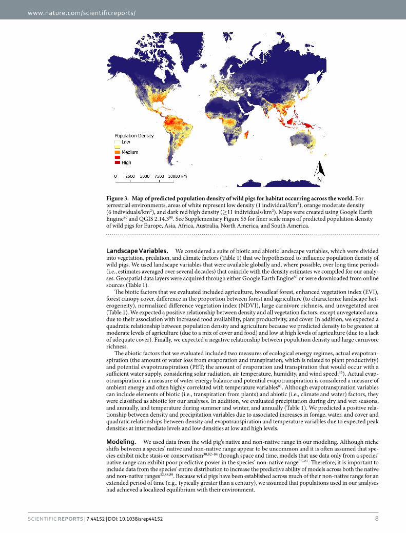
Using the full model-averaged results of parameter estimates, we created a predictive map of global wild pig population density (Fig. 3; Supplementary Figure S5). Wild pig populations were predicted to occur at low to high population densities across all continents, including large areas of land where wild pigs are currently absent. The highest predicted densities occurred in southeastern, eastern, and western North America, through-out Central America, northern, eastern, and southwestern South America, western, southern, and eastern Eurasia, throughout Indonesia, central and southern Africa, and northern and southeastern Australia (Fig. 3; Supplementary Figure S5). Results of k-fold cross validation demonstrated that the model had good predictive ability with a mean squared prediction error (MSPE) of 0.22 and a Pearson’s correlation between observed and predicted values of 0.80 (t = 17.711, df = 181, p-value < 0.001).

DiscussionPopulation density of an invasive large mammal was strongly influenced by both biotic and abiotic factors across its global distribution. Consistent with the prediction that abiotic factors drive broad-scale patterns of species distribution, potential evapotranspiration (PET) and precipitation variables were important predictors of popu-lation density on a global scale. In addition, contributing to growing evidence that biotic factors are also impor-tant determinants of broad-scale patterns of species distributions, both biotic interactions and vegetation played important roles in predicting the distribution of wild pig populations globally. Further, land-use change mediated by human activities strongly predicted the broad-scale distribution of an invasive large mammal. Consistent with previous studies evaluating how population density of ungulates varied across broad scales, both bottom-up (resource-related) and top-down (predation) factors influenced the distribution of wild pig populations19,42,43. Ultimately, wild pig populations across their global distribution appeared to respond to biotic and abiotic factors related to plant productivity, forage and water availability, cover, predation, and anthropogenic land-use change.

Using both biotic and abiotic factors to evaluate broad-scale species distributions can create more realistic maps of range and density with better predictive ability16,44, which can better inform management and conserva-tion strategies for species. For example, population density of wild pigs was highest in landscapes with moderate levels of agriculture and PET, lower large carnivore richness and amount of unvegetated area, and greater pre-cipitation during the wet and dry seasons. Using these relationships, we created a predictive map of population density across the world, which can be used to manage existing populations and predict areas where wild pig populations are likely to expand or invade if given the opportunity. Ultimately, this information can be used to prioritize management activities in areas at risk of invasion and with expanding populations.

Abiotic factors, such as temperature and precipitation, are consistently found to be primary determinants of species distributions at broad scales11. Potential evapotranspiration can be especially informative for understand-ing broad-scale ecological patterns45, such as species distributions. This was supported in our research where PET was the most important predictor of population density across the global distribution of wild pigs. Potential evap-otranspiration is highly correlated with temperature variables, thus indicating that wild pig density was greatest at relatively moderate temperatures and density was lower in areas exhibiting extreme low and high temperatures. In addition, the strong support of precipitation variables in our models is consistent with the association of wild pigs with vegetation cover, forage, and water36. In particular, precipitation likely facilitates rooting behavior by wild pigs by softening the soil substrate46.

Biotic factors were among the most supported variables predicting population density across a global scale. Our results indicated that the presence of large carnivores can influence wild pig population density. Large carni-vore richness was strongly supported in our models and exhibited a negative relationship with wild pig density; as the number of large carnivore species increased, wild pig density decreased, which is consistent with studies in

www.nature.com/scientificreports/

4Scientific RepoRts | 7:44152 | DOI: 10.1038/srep44152

Eurasia and Australia42,47,48. In addition, interspecific competition can influence the distribution of species and it has been hypothesized that wild pigs have not extensively invaded wildlands in some regions of sub-Saharan Africa due to the presence of other pig species that exhibit similar niches49. Although competition with other species might influence wild pig populations and their distribution49–51, in other cases wild pigs are reported to spatially and temporally partition habitat use to reduce niche overlap with potential competitors52–54 and not show evidence for interference competition with related mammals (e.g., species within the suborder Suiformes), such as native peccary species55, thus, it is unclear how interspecific interactions influence wild pig populations across their global distribution. Further, understanding potential interspecific competition for invasive species can be especially challenging in non-native habitat because invaders have not coevolved with competitors or predators and thus it is difficult to predict which species will be subordinate or dominant in potential competitive interactions or how competition might influence species distributions in unoccupied habitat17,18,56. Because it was

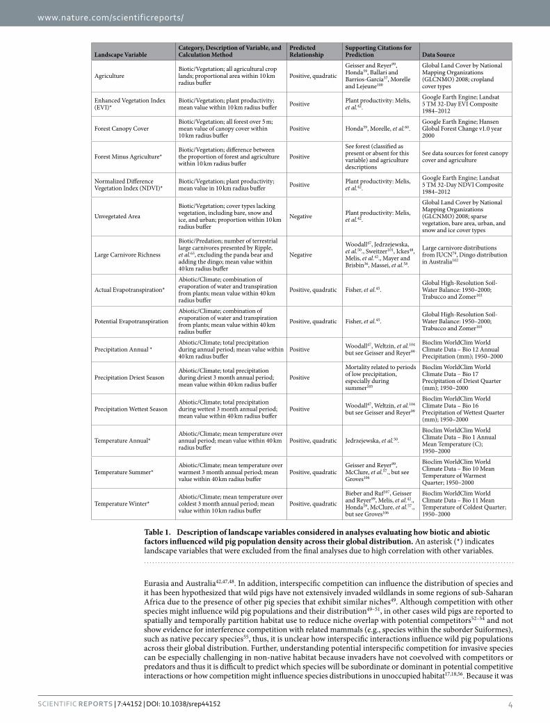
Landscape VariableCategory, Description of Variable, and Calculation Method

Predicted Relationship

Supporting Citations for Prediction Data Source

AgricultureBiotic/Vegetation; all agricultural crop lands; proportional area within 10 km radius buffer

Positive, quadraticGeisser and Reyer99, Honda59, Ballari and Barrios-García37, Morelle and Lejeune100

Global Land Cover by National Mapping Organizations (GLCNMO) 2008; cropland cover types

Enhanced Vegetation Index (EVI)*

Biotic/Vegetation; plant productivity; mean value within 10 km radius buffer Positive Plant productivity: Melis,

et al.42.Google Earth Engine; Landsat 5 TM 32-Day EVI Composite 1984–2012

Forest Canopy CoverBiotic/Vegetation; all forest over 5 m; mean value of canopy cover within 10 km radius buffer

Positive Honda59, Morelle, et al.60.Google Earth Engine; Hansen Global Forest Change v1.0 year 2000

Forest Minus Agriculture*Biotic/Vegetation; difference between the proportion of forest and agriculture within 10 km radius buffer

PositiveSee forest (classified as present or absent for this variable) and agriculture descriptions

See data sources for forest canopy cover and agriculture

Normalized Difference Vegetation Index (NDVI)*

Biotic/Vegetation; plant productivity; mean value in 10 km radius buffer Positive Plant productivity: Melis,

et al.42.Google Earth Engine; Landsat 5 TM 32-Day NDVI Composite 1984–2012

Unvegetated AreaBiotic/Vegetation; cover types lacking vegetation, including bare, snow and ice, and urban; proportion within 10 km radius buffer

Negative Plant productivity: Melis, et al.42.

Global Land Cover by National Mapping Organizations (GLCNMO) 2008; sparse vegetation, bare area, urban, and snow and ice cover types

Large Carnivore Richness

Biotic/Predation; number of terrestrial large carnivores presented by Ripple, et al.63, excluding the panda bear and adding the dingo; mean value within 40 km radius buffer

NegativeWoodall47, Jedrzejewska, et al.50., Sweitzer101, Ickes48, Melis, et al.42., Mayer and Brisbin36, Massei, et al.58.

Large carnivore distributions from IUCN79, Dingo distribution in Australia102

Actual Evapotranspiration*Abiotic/Climate; combination of evaporation of water and transpiration from plants; mean value within 40 km radius buffer

Positive, quadratic Fisher, et al.45.Global High-Resolution Soil-Water Balance: 1950–2000; Trabucco and Zomer103

Potential EvapotranspirationAbiotic/Climate; combination of evaporation of water and transpiration from plants; mean value within 40 km radius buffer

Positive, quadratic Fisher, et al.45.Global High-Resolution Soil-Water Balance: 1950–2000; Trabucco and Zomer103

Precipitation Annual *Abiotic/Climate; total precipitation during annual period; mean value within 40 km radius buffer

Positive Woodall47, Weltzin, et al.104 but see Geisser and Reyer99

Bioclim WorldClim World Climate Data – Bio 12 Annual Precipitation (mm); 1950–2000

Precipitation Driest SeasonAbiotic/Climate; total precipitation during driest 3 month annual period; mean value within 40 km radius buffer

PositiveMortality related to periods of low precipitation, especially during summer105

Bioclim WorldClim World Climate Data – Bio 17 Precipitation of Driest Quarter (mm); 1950–2000

Precipitation Wettest SeasonAbiotic/Climate; total precipitation during wettest 3 month annual period; mean value within 40 km radius buffer

Positive Woodall47, Weltzin, et al.104 but see Geisser and Reyer99

Bioclim WorldClim World Climate Data – Bio 16 Precipitation of Wettest Quarter (mm); 1950–2000

Temperature Annual*Abiotic/Climate; mean temperature over annual period; mean value within 40 km radius buffer

Positive, quadratic Jedrzejewska, et al.50.Bioclim WorldClim World Climate Data – Bio 1 Annual Mean Temperature (C); 1950–2000

Temperature Summer*Abiotic/Climate; mean temperature over warmest 3 month annual period; mean value within 40 km radius buffer

Positive, quadraticGeisser and Reyer99, McClure, et al.57., but see Groves106

Bioclim WorldClim World Climate Data – Bio 10 Mean Temperature of Warmest Quarter; 1950–2000

Temperature Winter*Abiotic/Climate; mean temperature over coldest 3 month annual period; mean value within 10 km radius buffer

Positive, quadraticBieber and Ruf107, Geisser and Reyer99, Melis, et al.42., Honda59, McClure, et al.57., but see Groves106

Bioclim WorldClim World Climate Data – Bio 11 Mean Temperature of Coldest Quarter; 1950–2000

Table 1. Description of landscape variables considered in analyses evaluating how biotic and abiotic factors influenced wild pig population density across their global distribution. An asterisk (*) indicates landscape variables that were excluded from the final analyses due to high correlation with other variables.

www.nature.com/scientificreports/

5Scientific RepoRts | 7:44152 | DOI: 10.1038/srep44152

unknown how competitive interactions between wild pigs and other species might influence their distribution, particularly outside their native range, competition was not included in our analyses. To understand how compe-tition between non-native and native species influences species distributions, field studies evaluating interspecific competition are necessary across the wild pig’s native and non-native geographic range, particularly across local spatial scales.

Although biotic interactions between animals are the primary biotic factors evaluated in species distribution models at broad scales, the role of plant communities has received less consideration. In particular, anthropogenic land-use change increasingly influences vegetation communities across continents and warrants a better under-standing for how human activities are shaping broad-scale distributions of plant and animal populations22,24. For example, agriculture is a dominating land cover type across continents23,25, which can potentially benefit species distributions in at least two ways. Agriculture can (1) increase population density within areas of a species’ cur-rent geographic range through supplemental food and increased resource availability and (2) allow geographic ranges to expand by creating habitat in areas that were previously unsuitable. In contrast, as agriculture increas-ingly dominates landscape patterns at broad extents, cover and other resources correspondingly decrease, which can negatively impact the geographic range and population density of some species. Our results demonstrate that agriculture can produce both positive and negative effects on populations, depending on the levels of agriculture. At intermediate levels of agriculture, population density of wild pigs was greatest, likely due to an optimal mix of food and cover. Whereas, at high levels of agriculture, population density decreased precipitously, which was likely a result of inadequate cover. Our results indicate that heterogeneous landscapes with a mix of agriculture and cover will support the greatest populations of wild pigs, which is consistent with broad-scale patterns of wild pig populations in North America and Eurasia57–59. Due to relatively high predicted population densities of wild pigs inhabiting heterogeneous landscapes, these regions would likely experience the greatest crop damage, lead-ing to high economic loss to farmers.

Forest is considered a key habitat type preferred by wild pigs59,60. In univariate analyses, forest was an impor-tant positive predictor of wild pig density (β = 0.170, se = 0.056). When considering additional predictor variables in our models, however, forest was relatively unimportant in predicting wild pig density, which is also consistent when evaluating wild pig occurrence over broad scales57. Thus, the interpretation of how forest influences the distribution of wild pigs must be considered in the context of other variables included in models, where abiotic factors might adequately explain forest distribution (see discussion below). However, as predicted, vegetation and cover play a strong role in predicting wild pig density; as the amount of unvegetated area increased across the landscape, wild pig population density decreased, which is consistent with geographic distribution maps of wild pigs61.

In some systems, abiotic factors can be stronger predictors of species distributions, than biotic factors, because of high correlations between these two factors62. Our study indicated that both factors can be important predic-tors of species distributions, potentially because abiotic factors may poorly predict biotic factors stemming from human activities. In addition, human influences might weaken the correlation between abiotic and biotic factors. For example, humans can significantly reduce the number of large carnivores in an area63, although these species would be predicted to occur across broad areas based on abiotic factors and historic biotic conditions. In addition, human land use change can lead to unpredictable biotic patterns in relation to abiotic factors, such as through agricultural landscape conversion. Although soil types might support crop production, many agricultural areas occur in arid landscapes requiring irrigation of water and application of fertilizer to maintain production25. Thus, agricultural crops could not grow in many areas based on broad-scale climate factors alone, and therefore, abiotic factors can be poor predictors of agricultural practices in some regions. Indeed, there likely are other examples where abiotic and biotic factors may exhibit low correlation in some systems (e.g., location of human activities and development, altered interspecific interactions due to human activities, and other forms of anthropogenic land use change). Ultimately, it can be useful to consider biotic factors in species distribution models that might be poorly predicted by abiotic factors due to human activities.

Additional biotic factors that can influences species distributions on a broad scale, particularly invasive species, include the role of humans in distributing the founding individuals of new populations. For example, invasive wild pig populations have arisen across several continents recently through human activities. Illegal translocations by humans for hunting purposes can facilitate the long-distance expansion of wild pig populations into new areas64–66, which is currently a primary source of new populations globally39,41. Further, in countries such as Canada, Brazil, and Sweden, wild pig farms were the propagule source for recent populations of wild pigs across broad regions, which are currently spreading into new areas67–69. Indeed, propagule pressure (i.e., the number of individuals introduced and release events) determines both the likelihood of invasive species becom-ing established, as well as the rate of geographic range expansion60,70. In addition, invasive species that exhibit r-selected characteristics (e.g., early maturity, short generation time, and high fecundity) can be more likely to successfully invade novel landscapes71. Even at low population densities, invasive species with high reproductive output are more likely to establish populations in areas of lower quality habitat72. Given that wild pigs are one of the most fecund large mammals (e.g., mean litter sizes ranging from 3.0 to 8.4 piglets per sow with the potential for > 1 litter annually)36, their reproductive characteristics might increase the probability of establishment and enable them to compensate for small population sizes when introduced into novel environments across a range of habitat qualities.

Population density, compared to presence-absence occurrence, can provide more informative conclusions of species distributions in relation to biotic and abiotic factors7,8. For example, although large carnivores likely do not exclude wild pigs from habitat across broad scales, our study revealed they can influence abundance. However, occurrence of species would remain constant across varying population densities, unless it resulted in species exclusion. Ultimately, population densities can provide more detailed information about species distribu-tions, which can better inform conservation and management plans and policy7. Studies analyzing presence-only

www.nature.com/scientificreports/

6Scientific RepoRts | 7:44152 | DOI: 10.1038/srep44152

data with logistic regression and Maximum Entropy (MaxEnt) models have examined methods to address spatial sampling bias73–75 and additional evaluations would be useful for studies using population density data with multiple linear regression. Further, global analyses of population genetics could be used to identify groups and the proportion of wild and domestic genes across wild pig populations, which could be used to incorporate pop-ulation structure into analyses to better understand population characteristics.

Predicting species distributions provides critical information to the management and conservation of bio-diversity, especially for controlling invasive species. Without intensive management actions, our study predicts that there is strong potential for wild pigs to expand their geographic range and further invade expansive areas of North America, South America, Africa, and Australia. Although wild pigs currently occupy broad regions of predicted habitat in their non-native range, many regions of predicted habitat are currently unoccupied and may be at high risk for future invasion. These areas might warrant increased surveillance by local, state, and federal agencies to counter the establishment of populations. Although attention in unoccupied areas that are predicted to support high densities of wild pigs might warrant priority for countering population introductions, wild pigs can persist in relatively low quality habitat (e.g., arid and/or cold regions) and these areas also warrant attention to halt invasions. Given the potential for wild pig populations to rapidly expand once established36, predictions of potential population density in unoccupied habitat can provide critical information to land managers, which can be used to proactively develop management plans to prevent introductions and control or eradicate populations if they become introduced.

MethodsDensity Estimates. To evaluate the population density (i.e., number of individuals per unit area) of wild pigs throughout their global distribution, we compiled density estimates from the literature throughout its native and non-native ranges across each continent and island for which data were available (Supplementary Table S1). Previous research evaluated how population density of wild pigs varied across western Eurasia42 and we incor-porated these 54 estimates of population density into our analysis. In addition, we followed the methodological recommendation of Melis et al.42. to average data when multiple estimates were available for > 1 season or year at a study area. Island populations typically exhibit higher population density compared to mainland popula-tions76,77. We thus compared estimates of wild pig population density between island and mainland populations; if population density for islands was significantly higher than on the mainland, we focused on only evaluating mainland populations in subsequent analyses.

Potential Evapotranspiration

Large Carnivore

Precipitation Wet Season Unvegetated Agriculture

Precipitation Dry Season Forest K AICc Δ AICc weight log(L)

* * * * * * 10 237.94 0.00 0.68 − 108.33

* * * * * * * 11 240.18 2.24 0.22 − 108.32

* * * * * 9 243.00 5.06 0.05 − 111.98

* * * * * * 10 244.40 6.46 0.03 − 111.56

* * * * * 8 246.14 8.20 0.01 − 114.65

* * * * * * 9 248.20 10.26 0.00 − 114.58

* * * * * 9 248.25 10.31 0.00 − 114.60

* * * * * * 10 249.14 11.20 0.00 − 113.93

* * * * * 9 252.95 15.01 0.00 − 116.95

* * * * 7 253.93 15.99 0.00 − 119.64

Table 2. Model selection results using Akaike Information Criteria (AICc) from analyses evaluating how population density of wild pigs was related to biotic and abiotic factors. A “*” in the covariate columns indicates whether the variable was included in the model. K is the number of variables included in the model. Note that Potential Evapotranspiration and Agriculture include both main and quadratic effects (thus accounting for two parameters for each of these variables). Only the top 10 models are reported. See Supplementary Table S4 for AICc model selection results of all possible variable combinations.

Potential Evapotranspiration

Large Carnivore

Precipitation Wet Season Unvegetated Agriculture

Precipitation Dry Season Forest

Variable Importance Values 1.00 1.00 1.00 0.99 0.98 0.92 0.25

Parameter Estimate (Standard Error)

m: 0.443 (0.056) q: − 0.226 (0.046) − 0.243 (0.043) 0.233 (0.055) − 0.203 (0.061) m: 0.236 (0.076)

q: − 0.118 (0.038) 0.100 (0.050) − 0.001 (0.029)

Table 3. Model selection results for parameters evaluating how population density of wild pigs is influenced by biotic and abiotic factors. Variable importance values sum model weights across the entire data set for each variable. Unconditional model-averaged parameter estimates with associated standard errors are based on standardized values. Potential Evapotranspiration and Agriculture include both main effect (m) and quadratic (q) terms, whereas all other covariates report linear relationships.

www.nature.com/scientificreports/

7Scientific RepoRts | 7:44152 | DOI: 10.1038/srep44152

Models evaluating and predicting species distributions can be improved by including areas of absence (a.k.a., pseudo-absence or background locations) or zero density to sample the full range of available landscape con-ditions1 to predict the potential range of a species, absence locations should occur outside the environmental domain of the species, but within a reasonable distance of the species’ geographic range78. Because wild pigs have occurred within their native range for thousands of years, we assumed that populations were at equilibrium and the species had colonized available habitat associated with its geographic distribution. Thus, regions adjacent to its native distribution that were classified as unoccupied were assumed to be unsuitable for population persistence due to unfavorable environmental conditions. In addition, spatial sampling bias (i.e., uneven sampling across geographic extents) can be addressed by increasing the number of background locations in areas with greater sampling73,74. The majority of density estimates used in our study occurred within the wild pig’s native range of Europe and Asia and we focused sampling of background locations associated with this region. To include loca-tions with estimates of zero density in our analyses, we used a three-step approach. First, we created a buffered region that occurred across the area between 100–1000 km around the boundary of the wild pig’s native range79. Next, we calculated the spatial extent of the native range and buffered regions. Lastly, accounting for the area of each region, we selected a random sample of locations within the buffered region that was proportional to the number of estimates used in the native terrestrial range of wild pigs. Based on this approach, we used 65 locations of zero density in our analyses that occurred across central Russia, Mongolia, western China, Saudi Arabia, and northern African countries. Zero density estimates were used in analyses relating wild pig density to landscape variables and excluded when comparing population density between island and mainland populations.

Figure 2. Relationships of biotic and abiotic factors with population density (natural log scale; #/km2) of wild pigs, including potential evapotranspiration (a), large carnivore richness (b), unvegetated (c), agriculture (d), precipitation during the wettest season (e), precipitation during the driest season (f), and forest canopy cover (g).

www.nature.com/scientificreports/

8Scientific RepoRts | 7:44152 | DOI: 10.1038/srep44152

Landscape Variables. We considered a suite of biotic and abiotic landscape variables, which were divided into vegetation, predation, and climate factors (Table 1) that we hypothesized to influence population density of wild pigs. We used landscape variables that were available globally and, where possible, over long time periods (i.e., estimates averaged over several decades) that coincide with the density estimates we compiled for our analy-ses. Geospatial data layers were acquired through either Google Earth Engine80 or were downloaded from online sources (Table 1).

The biotic factors that we evaluated included agriculture, broadleaf forest, enhanced vegetation index (EVI), forest canopy cover, difference in the proportion between forest and agriculture (to characterize landscape het-erogeneity), normalized difference vegetation index (NDVI), large carnivore richness, and unvegetated area (Table 1). We expected a positive relationship between density and all vegetation factors, except unvegetated area, due to their association with increased food availability, plant productivity, and cover. In addition, we expected a quadratic relationship between population density and agriculture because we predicted density to be greatest at moderate levels of agriculture (due to a mix of cover and food) and low at high levels of agriculture (due to a lack of adequate cover). Finally, we expected a negative relationship between population density and large carnivore richness.

The abiotic factors that we evaluated included two measures of ecological energy regimes, actual evapotran-spiration (the amount of water loss from evaporation and transpiration, which is related to plant productivity) and potential evapotranspiration (PET; the amount of evaporation and transpiration that would occur with a sufficient water supply, considering solar radiation, air temperature, humidity, and wind speed;45). Actual evap-otranspiration is a measure of water-energy balance and potential evapotranspiration is considered a measure of ambient energy and often highly correlated with temperature variables81. Although evapotranspiration variables can include elements of biotic (i.e., transpiration from plants) and abiotic (i.e., climate and water) factors, they were classified as abiotic for our analyses. In addition, we evaluated precipitation during dry and wet seasons, and annually, and temperature during summer and winter, and annually (Table 1). We predicted a positive rela-tionship between density and precipitation variables due to associated increases in forage, water, and cover and quadratic relationships between density and evapotranspiration and temperature variables due to expected peak densities at intermediate levels and low densities at low and high levels.

Modeling. We used data from the wild pig’s native and non-native range in our modeling. Although niche shifts between a species’ native and non-native range appear to be uncommon and it is often assumed that spe-cies exhibit niche stasis or conservatism30,82–84 through space and time, models that use data only from a species’ native range can exhibit poor predictive power in the species’ non-native range85–87. Therefore, it is important to include data from the species’ entire distribution to increase the predictive ability of models across both the native and non-native ranges32,88,89. Because wild pigs have been established across much of their non-native range for an extended period of time (e.g., typically greater than a century), we assumed that populations used in our analyses had achieved a localized equilibrium with their environment.

Figure 3. Map of predicted population density of wild pigs for habitat occurring across the world. For terrestrial environments, areas of white represent low density (1 individual/km2), orange moderate density (6 individuals/km2), and dark red high density (≥ 11 individuals/km2). Maps were created using Google Earth Engine80 and QGIS 2.14.390. See Supplementary Figure S5 for finer scale maps of predicted population density of wild pigs for Europe, Asia, Africa, Australia, North America, and South America.

www.nature.com/scientificreports/

9Scientific RepoRts | 7:44152 | DOI: 10.1038/srep44152

All geospatial data layers were evaluated using QGIS90 and Google Earth Engine80 and statistical analyses were conducted using R91. Because there is uncertainty about the exact location of studies and the scale in which processes might influence wild pig densities, we evaluated multiple scales for each covariate using 10, 20, and 40 km radius buffers around the location of each density estimate (Table 1). Thus a moving window approach was conducted so that each pixel within a spatial layer summarized the landscape within the buffered radius. To determine the best scale for analyses we used a multi-criteria approach. First, variables were centered and scaled to improve model fit92. Next, we considered quadratic relationships for landscape factors that were predicted to exhibit a curvilinear pattern (Table 1). Last, we selected the best scale and relationship for each covariate based on wild pig ecology, model comparisons using Akaike’s Information Criterion corrected for small sample size AICc;93, and plots of residuals. Once the appropriate scale was determined for each variable (Table 1), we eval-uated the Pearson correlation among all variables and excluded highly correlated variables (r > 0.70) from our final analysis.

We used multiple linear regression to evaluate how population density was influenced by our final suite of biotic and abiotic factors (Table 1). The distribution of density estimates were right skewed, thus we log-transformed density estimates using the natural logarithm42. To compare the relative importance of biotic and abiotic factors and to determine parameter estimates of variables, we ranked all possible models using AICc, model-averaged parameter estimates (i.e., full conditional), and calculated variable importance values93–95. We used model weights and evidence ratios to evaluate if biotic factors improved model fit by comparing models including only abiotic factors to models also including biotic factors. Model averaged parameter estimates were used to create a predictive global map of wild pig density (1 km2 resolution). This map displays the maximal potential density of wild pigs in relation to the biotic and abiotic factors used in our modeling and reflects pre-dicted densities that would be achieved if wild pigs had access to all landscapes, their movements were unre-stricted, and management activities did not suppress populations. We validated our model using mean squared prediction error (MSPE)96 and k-fold cross validation and selected the number of bins based on Huberty’s rule of thumb (k = 4)97.

References1. Franklin, J. Mapping species distributions: spatial inference and prediction. (Cambridge University Press, 2009).2. Grinnell, J. The niche-relationships of the California Thrasher. The Auk 34, 427–433 (1917).3. MacArthur, R. H. In Population Biology and Evolution (ed R. C. Lewontin) 159–186 (Syracuse University Press, 1968).4. Hutchinson, G. E. Concluding remarks. Cold Spring Harbor Symposium on Quantitative Biology 22, 415–427 (1957).5. Brown, J. H. Macroecology: progress and prospect. Oikos 87, 3–14 (1999).6. Elith, J. & Leathwick, J. R. Species distribution models: ecological explanation and prediction across space and time. Annual Review

of Ecology, Evolution, and Systematics 40, 677–697 (2009).7. Brown, J. H., Mehlman, D. W. & Stevens, G. C. Spatial variation in abundance. Ecology 76, 2028–2043 (1995).8. Randin, C. F., Jaccard, H., Vittoz, P., Yoccoz, N. G. & Guisan, A. Land use improves spatial predictions of mountain plant

abundance but not presence-absence. Journal of Vegetation Science 20, 996–1008 (2009).9. Pearson, R. G. & Dawson, T. P. Predicting the impacts of climate change on the distribution of species: are bioclimate envelope

models useful? Global Ecology and Biogeography 12, 361–371 (2003).10. Benton, M. J. The Red Queen and the Court Jester: species diversity and the role of biotic and abiotic factors through time. Science

323, 728–732 (2009).11. Wiens, J. J. The niche, biogeography and species interactions. Philosophical Transactions of the Royal Society of London B: Biological

Sciences 366, 2336–2350 (2011).12. Van der Putten, W. H., Macel, M. & Visser, M. E. Predicting species distribution and abundance responses to climate change: why

it is essential to include biotic interactions across trophic levels. Philosophical Transactions of the Royal Society B: Biological Sciences 365, 2025–2034 (2010).

13. Meier, E. S. et al. Biotic and abiotic variables show little redundancy in explaining tree species distributions. Ecography 33, 1038–1048 (2010).

14. Guisan, A. & Thuiller, W. Predicting species distribution: offering more than simple habitat models. Ecology Letters 8, 993–1009 (2005).

15. Wisz, M. S. et al. The role of biotic interactions in shaping distributions and realised assemblages of species: implications for species distribution modelling. Biological Reviews 88, 15–30 (2013).

16. Leach, K., Montgomery, W. I. & Reid, N. Modelling the influence of biotic factors on species distribution patterns. Ecological Modelling 337, 96–106 (2016).

17. Anderson, R. P. When and how should biotic interactions be considered in models of species niches and distributions? Journal of Biogeography, doi: 10.1111/jbi.12825 (2016).

18. Sexton, J. P., McIntyre, P. J., Angert, A. L. & Rice, K. J. Evolution and ecology of species range limits. Annual Review of Ecology, Evolution, and Systematics 40, 415–436 (2009).

19. Melis, C. et al. Predation has a greater impact in less productive environments: variation in roe deer, Capreolus capreolus, population density across Europe. Global Ecology and Biogeography 18, 724–734 (2009).

20. Pasanen-Mortensen, M., Pyykönen, M. & Elmhagen, B. Where lynx prevail, foxes will fail–limitation of a mesopredator in Eurasia. Global Ecology and Biogeography 22, 868–877 (2013).

21. Boulangeat, I., Gravel, D. & Thuiller, W. Accounting for dispersal and biotic interactions to disentangle the drivers of species distributions and their abundances. Ecology Letters 15, 584–593 (2012).

22. Sanderson, E. W. et al. The Human Footprint and the Last of the Wild. Bioscience 52, 891–904 (2002).23. Laurance, W. F., Sayer, J. & Cassman, K. G. Agricultural expansion and its impacts on tropical nature. Trends in Ecology & Evolution

29, 107–116 (2014).24. Newbold, T. et al. Global effects of land use on local terrestrial biodiversity. Nature 520, 45–50 (2015).25. Alexandratos, N. & Bruinsma, J. World agriculture towards 2030/2050: the 2012 revision. (ESA Working Paper No. 12-03, Rome,

FAO, 2012).26. Green, R. E., Cornell, S. J., Scharlemann, J. P. & Balmford, A. Farming and the fate of wild nature. Science 307, 550–555 (2005).27. Bengtsson, J., Ahnström, J. & Weibull, A.-C. The effects of organic agriculture on biodiversity and abundance: a meta-analysis.

Journal of Applied Ecology 42, 261–269 (2005).28. Mack, R. N. et al. Biotic invasions: causes, epidemiology, global consequences, and control. Ecological Applications 10, 689–710

(2000).

www.nature.com/scientificreports/

1 0Scientific RepoRts | 7:44152 | DOI: 10.1038/srep44152

29. Parmesan, C. et al. Empirical perspectives on species borders: from traditional biogeography to global change. Oikos 108, 58–75 (2005).

30. Peterson, A. T. Predicting the geography of species’ invasions via ecological niche modeling. The Quarterly Review of Biology 78, 419–433 (2003).

31. Ficetola, G. F., Thuiller, W. & Miaud, C. Prediction and validation of the potential global distribution of a problematic alien invasive species—the American bullfrog. Diversity and Distributions 13, 476–485 (2007).

32. Sánchez-Fernández, D., Lobo, J. M. & Hernández-Manrique, O. L. Species distribution models that do not incorporate global data misrepresent potential distributions: a case study using Iberian diving beetles. Diversity and Distributions 17, 163–171 (2011).

33. Kauhala, K. & Kowalczyk, R. Invasion of the raccoon dog Nyctereutes procyonoides in Europe: history of colonization, features behind its success, and threats to native fauna. Current Zoology 57, 584–598 (2011).

34. Oliver, W. L. R. & Brisbin, I. In Pigs, peccaries and Hippos: status survey and conservation action plan (ed W. L. R. Oliver) 179–195 (IUCN, 1993).

35. Oliver, W. L. R., Brisbin, I. L. & Takahashi, S. In Pigs, peccaries and Hippos: status survey and conservation action plan (ed W. L. R. Oliver) 112–120 (IUCN, 1993).

36. Mayer, J. & Brisbin, I. L. Wild pigs: biology, damage, control techniques and management. (Savannah River Site Aiken, SC, USA, 2009).

37. Ballari, S. A. & Barrios-García, M. N. A review of wild boar Sus scrofa diet and factors affecting food selection in native and introduced ranges. Mammal Review 44, 124–134 (2014).

38. Lowe, S., Browne, M., Boudjelas, S. & De Poorter, M. 100 of the world’s worst invasive alien species: A selection from the global invasive species database. 1–12 (Aukland, New Zealand, 2000).

39. Barrios-Garcia, M. N. & Ballari, S. A. Impact of wild boar (Sus scrofa) in its introduced and native range: a review. Biological Invasions 14, 2283–2300 (2012).

40. Courchamp, F., Chapuis, J.-L. & Pascal, M. Mammal invaders on islands: impact, control and control impact. Biological Reviews 78, 347–383 (2003).

41. Bevins, S. N., Pedersen, K., Lutman, M. W., Gidlewski, T. & Deliberto, T. J. Consequences associated with the recent range expansion of nonnative feral swine. Bioscience 64, 291–299 (2014).

42. Melis, C., Szafrańska, P. A., Jędrzejewska, B. & Bartoń, K. Biogeographical variation in the population density of wild boar (Sus scrofa) in western Eurasia. Journal of Biogeography 33, 803–811 (2006).

43. Danell, K., Bergström, R., Duncan, P. & Pastor, J. Large herbivore ecology, ecosystem dynamics and conservation. Vol. 11 (Cambridge University Press, 2006).

44. González-Salazar, C., Stephens, C. R. & Marquet, P. A. Comparing the relative contributions of biotic and abiotic factors as mediators of species’ distributions. Ecological Modelling 248, 57–70 (2013).

45. Fisher, J. B., Whittaker, R. J. & Malhi, Y. ET come home: potential evapotranspiration in geographical ecology. Global Ecology and Biogeography 20, 1–18 (2011).

46. Sandom, C. J., Hughes, J. & Macdonald, D. W. Rooting for rewilding: quantifying wild boar’s Sus scrofa rooting rate in the Scottish Highlands. Restoration Ecology 21, 329–335 (2013).

47. Woodall, P. F. Distribution and population dynamics of dingoes (Canis familiaris) and feral pigs (Sus scrofa) in Queensland, 1945-1976. Journal of Applied Ecology 20, 85–95 (1983).

48. Ickes, K. Hyper-abundance of native wild pigs (Sus scrofa) in a lowland Dipterocarp rain forest of peninsular Malaysia Biotropica 33, 682–690 (2001).

49. Oliver, W. & Fruzinski, B. In Biology of Suidae (eds R. H. Barrett & F. Spitz) 93–116 (Institute National de Recherche Agronomique, Castanet, France, 1991).

50. Jedrzejewska, B., Jedrzejewski, W., Bunevich, A. N., Milkowski, L. & Krasinski, Z. A. Factors shaping population densities and increase rates of ungulates in Bialowieza Primeval Forest (Poland and Belarus) in the 19th and 20th centuries. Acta Theriologica 42, 399–451 (1997).

51. Corbett, L. Does dingo predation or buffalo competition regulate feral pig populations in the Australian wet-dry tropics? An experimental study. Wildlife Research 22, 65–74 (1995).

52. Ilse, L. M. & Hellgren, E. C. Resource partitioning in sympatric populations of collared peccaries and feral hogs in southern Texas. Journal of Mammalogy 76, 784–799 (1995).

53. Desbiez, A. L. J., Santos, S. A., Keuroghlian, A. & Bodmer, R. E. Niche partitioning among white-lipped peccaries (Tayassu pecari), collared peccaries (Pecari tajacu), and feral pigs (Sus scrofa). Journal of Mammalogy 90, 119–128 (2009).

54. Gabor, T. M., Hellgren, E. C. & Silvy, N. J. Multi-scale habitat partitioning in sympatric suiforms. The Journal of Wildlife Management 65, 99–110 (2001).

55. Oliveira-Santos, L. G., Dorazio, R. M., Tomas, W. M., Mourao, G. & Fernandez, F. A. No evidence of interference competition among the invasive feral pig and two native peccary species in a Neotropical wetland. Journal of Tropical Ecology 27, 557–561 (2011).

56. Louthan, A. M., Doak, D. F. & Angert, A. L. Where and when do species interactions set range limits? Trends in Ecology & Evolution 30, 780–792 (2015).

57. McClure, M. L. et al. Modeling and mapping the probability of occurrence of invasive wild pigs across the contiguous United States. PLoS ONE 10, e0133771 (2015).

58. Massei, G. et al. Wild boar populations up, numbers of hunters down? A review of trends and implications for Europe. Pest Management Science 71, 492–500 (2015).

59. Honda, T. Environmental factors affecting the distribution of the wild boar, sika deer, Asiatic black bear and Japanese macaque in central Japan, with implications for human-wildlife conflict. Mammal Study 34, 107–116 (2009).

60. Morelle, K., Fattebert, J., Mengal, C. & Lejeune, P. Invading or recolonizing? Patterns and drivers of wild boar population expansion into Belgian agroecosystems. Agriculture, Ecosystems & Environment 222, 267–275 (2016).

61. Oliver, W. & Leus, K. Sus scrofa. The IUCN Red List of Threatened Species 2008: e.T41775A10559847. http://dx.doi.org/10.2305/IUCN.UK.2008.RLTS.T41775A10559847.en. (2008).

62. Godsoe, W., Franklin, J. & Blanchet, F. G. Effects of biotic interactions on modeled species’ distribution can be masked by environmental gradients. Ecology and Evolution 7, 654–664 (2017).

63. Ripple, W. J. et al. Status and ecological effects of the world’s largest carnivores. Science 343, 1241484 (2014).64. Spencer, P. B. & Hampton, J. O. Illegal translocation and genetic structure of feral pigs in Western Australia. Journal of Wildlife

Management 69, 377–384 (2005).65. Skewes, O. & Jaksic, F. M. History of the introduction and present distribution of the european wild boar (Sus scrofa) in Chile.

Mastozoología Neotropical 22, 113–124 (2015).66. Gipson, P. S., Hlavachick, B. & Berger, T. Range expansion by wild hogs across the central United States. Wildlife Society (USA)

(1998).67. Brook, R. K. & van Beest, F. M. Feral wild boar distribution and perceptions of risk on the central Canadian prairies. Wildlife

Society Bulletin 38, 486–494 (2014).68. Pedrosa, F., Salerno, R., Padilha, F. V. B. & Galetti, M. Current distribution of invasive feral pigs in Brazil: economic impacts and

ecological uncertainty. Natureza & Conservação 13, 84–87 (2015).

www.nature.com/scientificreports/

1 1Scientific RepoRts | 7:44152 | DOI: 10.1038/srep44152

69. Lemel, J., Truvé, J. & Söderberg, B. Variation in ranging and activity behaviour of European wild boar Sus scrofa in Sweden. Wildlife Biology 9, 29–36 (2003).

70. Lockwood, J. L., Cassey, P. & Blackburn, T. The role of propagule pressure in explaining species invasions. Trends in Ecology & Evolution 20, 223–228 (2005).

71. Sakai, A. K. et al. The population biology of invasive specie. Annual Review of Ecology and Systematics 32, 305–332 (2001).72. Warren, R. J., Bahn, V. & Bradford, M. A. The interaction between propagule pressure, habitat suitability and density-dependent

reproduction in species invasion. Oikos 121, 874–881 (2012).73. Syfert, M. M., Smith, M. J. & Coomes, D. A. The effects of sampling bias and model complexity on the predictive performance of

MaxEnt species distribution models. PLoS ONE 8, e55158 (2013).74. Barbet-Massin, M., Jiguet, F., Albert, C. H. & Thuiller, W. Selecting pseudo-absences for species distribution models: how, where

and how many? Methods in Ecology and Evolution 3, 327–338 (2012).75. Kramer-Schadt, S. et al. The importance of correcting for sampling bias in MaxEnt species distribution models. Diversity and

Distributions 19, 1366–1379 (2013).76. Adler, G. H. & Levins, R. The island syndrome in rodent populations. Quarterly Review of Biology 69, 473–490 (1994).77. Krebs, C. J., Keller, B. L. & Tamarin, R. H. Microtus population biology: demographic changes in fluctuating populations of M.

ochrogaster and M. pennsylvanicus in southern Indiana. Ecology 50, 587–607 (1969).78. Lobo, J. M., Jiménez-Valverde, A. & Hortal, J. The uncertain nature of absences and their importance in species distribution

modelling. Ecography 33, 103–114 (2010).79. IUCN. The IUCN Red List of Threatened Species. Version 2014.1. http://www.iucnredlist.org. Downloaded on 26 February 2016.

(2014).80. Google Earth Engine Team. Google Earth Engine: A planetary-scale geospatial analysis platform. https://earthengine.google.com/.

(2016).81. Hawkins, B. A. et al. Energy, water, and broad-scale geographic patterns of species richness. Ecology 84, 3105–3117 (2003).82. Wiens, J. J. et al. Niche conservatism as an emerging principle in ecology and conservation biology. Ecology Letters 13, 1310–1324

(2010).83. Wiens, J. J. & Graham, C. H. Niche conservatism: integrating evolution, ecology, and conservation biology. Annual Review of

Ecology, Evolution, and Systematics 36, 519–539 (2005).84. Alexander, J. M. & Edwards, P. J. Limits to the niche and range margins of alien species. Oikos 119, 1377–1386 (2010).85. Fitzpatrick, M. C., Weltzin, J. F., Sanders, N. J. & Dunn, R. R. The biogeography of prediction error: why does the introduced range

of the fire ant over-predict its native range? Global Ecology and Biogeography 16, 24–33 (2007).86. Mau-Crimmins, T. M., Schussman, H. R. & Geiger, E. L. Can the invaded range of a species be predicted sufficiently using only

native-range data?: Lehmann lovegrass (Eragrostis lehmanniana) in the southwestern United States. Ecological Modelling 193, 736–746 (2006).

87. Loo, S. E., Nally, R. M. & Lake, P. Forecasting New Zealand mudsnail invasion range: model comparisons using native and invaded ranges. Ecological Applications 17, 181–189 (2007).

88. Broennimann, O. & Guisan, A. Predicting current and future biological invasions: both native and invaded ranges matter. Biology Letters 4, 585–589 (2008).

89. Beaumont, L. J. et al. Different climatic envelopes among invasive populations may lead to underestimations of current and future biological invasions. Diversity and Distributions 15, 409–420 (2009).

90. QGIS Development Team. QGIS 2.14.3 Geographic Information System. Open Source Geospatial Foundation Project. http://qgis.osgeo.org. (2016).

91. R. R: a language and environment for statistical computing, Version 3.2.3. R Foundation for Statistical Computing. Vienna, Austria. (Development Core Team 2016).

92. Schielzeth, H. Simple means to improve the interpretability of regression coefficients. Methods in Ecology and Evolution 1, 103–113 (2010).

93. Burnham, K. P. & Anderson, D. R. Model selection and multimodel inference: a practical information-theoretic approach. Second Edition., (Springer Verlag, 2002).

94. Doherty, P. F., White, G. C. & Burnham, K. P. Comparison of model building and selection strategies. Journal of Ornithology 152, 317–323 (2012).

95. Lukacs, P. M., Burnham, K. P. & Anderson, D. R. Model selection bias and Freedman’s paradox. Annals of the Institute of Statistical Mathematics 62, 117–125 (2010).

96. Murtaugh, P. A. Performance of several variable-selection methods applied to real ecological data. Ecology Letters 12, 1061–1068 (2009).

97. Boyce, M. S., Vernier, P. R., Nielsen, S. E. & Schmiegelow, F. K. Evaluating resource selection functions. Ecological Modelling 157, 281–300 (2002).

98. ESRI. ArcGIS Desktop: Version 10.3.1 Environmental Systems Research Institute, Redlands, CA, USA. (2015).99. Geisser, H. & Reyer, H.-u. The influence of food and temperature on population density of wild boar Sus scrofa in the Thurgau

(Switzerland). Journal of Zoology 267, 89–96 (2005).100. Morelle, K. & Lejeune, P. Seasonal variations of wild boar Sus scrofa distribution in agricultural landscapes: a species distribution

modelling approach. European Journal of Wildlife Research 61, 45–56 (2015).101. Sweitzer, R. A. Conservation implications of feral pigs in island and mainland ecosystems, and a case study of feral pig expansion

in California. Proceedings of 18th Vertebrate Pest Conference 18 26–34 (1998).102. Fleming, P. J. et al. In Carnivores of Australia: past, present and future (eds A. S. Glen & C. R. Dickman) (CSIRO Publishing, 2014).103. Trabucco, A. & Zomer, R. Global soil water balance geospatial database. CGIAR Consortium for Spatial Information. Published

online, available from the CGIARCSI GeoPortal at http://cgiar-csi. org (2010).104. Weltzin, J. F. et al. Assessing the response of terrestrial ecosystems to potential changes in precipitation. Bioscience 53, 941–952

(2003).105. Massei, G., Genov, P., Staines, B. & Gorman, M. Mortality of wild boar, Sus scrofa, in a Mediterranean area in relation to sex and

age. Journal of Zoology 242, 394–400 (1997).106. Groves, C. P. Ancestors for the pigs: taxonomy and phylogeny of the genus Sus. 1–96 (Dept. of Prehistory, Australian National

University, 1981).107. Bieber, C. & Ruf, T. Population dynamics in wild boar Sus scrofa: ecology, elasticity of growth rate and implications for the

management of pulsed resource consumers. Journal of Applied Ecology 42, 1203–1213 (2005).

AcknowledgementsThis study was funded and supported by the US Department of Agriculture, Animal and Plant Health Inspection Service, Center for Epidemiology and Animal Health, Veterinary Services, Wildlife Services, the National Wildlife Research Center, the National Feral Swine Damage Management Program, Colorado State University, and Conservation Science Partners. We appreciate the distribution data for wild pigs in Canada provided by R. Kost and R. Brook, synthesis of wild pig distribution in Africa and South America by C. Larson, and the dingo

www.nature.com/scientificreports/

1 2Scientific RepoRts | 7:44152 | DOI: 10.1038/srep44152

distribution data in Australia provided by P. Fleming. P. DiSalvo and M. Foley assisted with acquiring literature on density estimates. M. McClure assisted with cross validation of model results. We thank three anonymous reviewers, S. Sweeney and B. Dickson for providing thoughtful feedback that improved earlier versions of this paper.

Author ContributionsJ.L. conceived the ideas, led the analyses, and wrote the manuscript. C.B., M.F., M.G., R.M., and D.T. contributed to the development of ideas, assisted with analyses, and edited the manuscript. CB created the large carnivore richness GIS layer and wild pig global range figure.

Additional InformationSupplementary information accompanies this paper at http://www.nature.com/srepCompeting Interests: The authors declare no competing financial interests.How to cite this article: Lewis, J. S. et al. Biotic and abiotic factors predicting the global distribution and population density of an invasive large mammal. Sci. Rep. 7, 44152; doi: 10.1038/srep44152 (2017).Publisher's note: Springer Nature remains neutral with regard to jurisdictional claims in published maps and institutional affiliations.

This work is licensed under a Creative Commons Attribution 4.0 International License. The images or other third party material in this article are included in the article’s Creative Commons license,

unless indicated otherwise in the credit line; if the material is not included under the Creative Commons license, users will need to obtain permission from the license holder to reproduce the material. To view a copy of this license, visit http://creativecommons.org/licenses/by/4.0/ © The Author(s) 2017

Biotic and abiotic factors predicting the global distribution and population density of an

invasive large mammal

Jesse S. Lewis1*, Matthew L. Farnsworth1, Chris L. Burdett2, David M. Theobald1, Miranda

Gray3, Ryan S. Miller4

Supplementary Files 1, 2, 3, 4, and 5

1 Conservation Science Partners, 5 Old Town Sq, Suite 205, Fort Collins, Colorado, USA 80524,

jlewis@csp-inc.org, matthew.l.farnsworth@gmail.com, davet@csp-inc.org

2 Colorado State University, Department of Biology, Fort Collins, Colorado, USA 80524,

chris.burdett@colostate.edu

3 Conservation Science Partners, c, Truckee, California, USA 96161, miranda@csp-inc.org

4 United States Department of Agriculture, Animal and Plant Health Inspection Service,

Veterinary Services, Center for Epidemiology and Animal Health, Fort Collins, Colorado, USA

80524, ryan.s.miller@aphis.usda.gov

* Corresponding author: Jesse S Lewis; jslewis.research@gmail.com; telephone (970) 484 – 2898

Supplementary Methods S1. Methods and studies used to create the global distribution map of

wild pigs across large land areas within their native and non-native range (Figure 1).

Methods

We mapped the extent of occurrence of wild pigs by first compiling existing spatial datasets

depicting Sus scrofa’s geographic range 1,2. Second, we created additional spatial data by

digitizing range maps or known occurrence locations from publications. We paid particular

attention to range boundaries and areas where their distribution was poorly understood. To

upscale fine-grained spatial data digitized from publications into a similar resolution as the

existing broad-scale range maps, we buffered point locations by 10 km and then intersected the

buffered points or polygons with Pfafstetter Level 6 watersheds obtained from the HydroSHEDS

spatial hydrography database 3,4. We used watersheds to spatially filter these data because they

provide a biologically meaningful way to depict the presence of wild pigs at a landscape-scale

resolution 5. Lastly, we differentiated two categories of occurrence, areas where the presence of

wild pigs has been confirmed through published maps or data, and other areas where the

occurrence of wild pigs is less certain. All digitizing and map development was performed using

ArcGIS software 6.

Studies used in constructing distribution

Global

Oliver and Brisbin 7, Long 8, Meijaard, et al. 9, Barrios-Garcia and Ballari 10

Eurasia

Erkinaro, et al. 11, Oliver and Leus 12, Campbell and Hartley 13, Magnusson 14, NBDCI 15,

Haaverstad, et al. 16, IUCN 2, Ukkonen, et al. 17, Wilson 18

Africa

Blench 19, Phiri, et al. 20, Kisakye and Masaba 21, Pouedet, et al. 22, Ngowi, et al. 23, Githigia, et

al. 24, Waiswa, et al. 25, Assana, et al. 26, Kingdon and Hoffmann 27, Thomas, et al. 28, Ouma, et

al. 29

Australia

West 30

United States and Canada

SCWDS 31, Ruth Kost and Ryan Brook, University of Saskatchewan, personal communication

Mexico

Álvarez-Romero, et al. 32, Solís-Cámara, et al. 33, Hidalgo-Mihart, et al. 34

South America

Merino and Carpinetti 35, Merino, et al. 36, Desbiez, et al. 37, Desbiez, et al. 38, Salvador and

Fernandez 39, Kaizer, et al. 40, Aravena, et al. 41, Ballari, et al. 42, Pedrosa, et al. 43, Skewes and

Jaksic 44

References

1 Saulich, M. I. in Interactive Agricultural Ecological Atlas of Russia and Neighboring

Countries. Economic Plants and their Diseases, Pests and Weeds [Online]. (eds A.N.

Afonin, S.L. Greene, N.I. Dzyubenko, & A.N. Frolov) (Available at:

http://www.agroatlas.ru/en/content/pests/Sus_scrofa/map/, 2007).

2 IUCN. The IUCN Red List of Threatened Species. Version 2014.1.

http://www.iucnredlist.org. Downloaded on 26 February 2016. (2014).

3 Lehner, B., Verdin, K. & Jarvis, A. New global hydrography derived from spaceborne

elevation data. Eos 89, 93-94 (2008).

4 Lehner, B. & Grill, G. Global river hydrography and network routing: baseline data and

new approaches to study the world's large river systems. Hydrological Processes 27,

2171-2186, doi:10.1002/hyp.9740 (2013).

5 McClure, M. L. et al. Modeling and Mapping the Probability of Occurrence of Invasive

Wild Pigs across the Contiguous United States. PLoS ONE 10, e0133771,

doi:10.1371/journal.pone.0133771 (2015).

6 ESRI. ArcGIS Desktop: Version 10.3.1 Environmental Systems Research Institute,

Redlands, CA, USA. (2015).

7 Oliver, W. & Brisbin, I. L. Introduced and feral pigs: problems, policy, and priorities.

Pigs, peccaries and hippos. International Union Conservation of Nature and Natural

Resources, Gland, Switzerland, 179-191 (1993).

8 Long, J. L. Introduced mammals of the world: their history, distribution and influence.

(Csiro Publishing, 2003).

9 Meijaard, E., d'Huart, J. P. & Oliver, W. L. R. Family Suidae (Pigs). Handbook of the

mammals of the world, 2. Hoofed Mammals. 248-292 (Lynx Edicions, 2011).

10 Barrios-Garcia, M. N. & Ballari, S. A. Impact of wild boar (Sus scrofa) in its introduced

and native range: a review. Biological Invasions 14, 2283-2300 (2012).

11 Erkinaro, E., Heikura, K., Lindgren, E., Pulliainen, E. & Sulkava, S. Occurrence and

spread of the wild boar (Sus scrofa) in eastern Fennoscandia. Memoranda Societas Fauna

et Flora Fennica 58, 39-47 (1982).

12 Oliver, W. & Leus, K. Sus scrofa. The IUCN Red List of Threatened Species 2008:

e.T41775A10559847.

http://dx.doi.org/10.2305/IUCN.UK.2008.RLTS.T41775A10559847.en. . (2008).

13 Campbell, S. & Hartley, G. Wild boar distribution in Scotland. Poster presentation. 8th

International Symposium on Wild Boar and Other Suids. Available at

https://www.sasa.gov.uk/content/wild-boar-distribution-scotland (2010).

14 Magnusson, M. Population and management models for the Swedish wild boar (Sus

scrofa). . Master’s Thesis. Swedish University of Agricultural Sciences, Sweden

(http://stud.espsilon.slu.se) (2010).

15 NBDCI. National Biodiversity Data Centre (Ireland). Sus scrofa biodiversity map.

Available at: http://www.biodiversityireland.ie/wild-boar-hybridferal-pig/. (2012).

16 Haaverstad, O., Hjeljord, O. & Wam, H. K. Wild boar rooting in a northern coniferous

forest – minor silviculture impact. Scandinavian Journal of Forest Research 29, 90-95,

doi:10.1080/02827581.2013.865781 (2014).

17 Ukkonen, P., Mannermaa, K. & Nummi, P. New evidence of the presence of wild boar

(Sus scrofa) in Finland during early Holocene: Dispersal restricted by snow and hunting?

The Holocene, 0959683614557575 (2014).

18 Wilson, C. J. The establishment and distribution of feral wild boar (Sus scrofa) in

England. Wildlife Biology in Practice 10, 1-6 (2014).

19 Blench, R. M. in The origins and development of African Livestock: Archaeology,

genetics, linguistics, and ethnography (eds Roger M Blench & Kevin C MacDonald)

355-367 (Routledge, 2000).

20 Phiri, I. K. et al. The prevalence of porcine cysticercosis in Eastern and Southern

provinces of Zambia. Veterinary Parasitology 108, 31-39,

doi:http://dx.doi.org/10.1016/S0304-4017(02)00165-6 (2002).

21 Kisakye, J. & Masaba, S. Cysticcrcus ccllulosae in pigs slaughtered in and around

Kampala city. Uganda Journal of Agricultural Sciences 2, 23-24 (2002).

22 Pouedet, M. S. R. et al. Epidemiological survey of swine cysticercosis in two rural

communities of West-Cameroon. Veterinary Parasitology 106, 45-54,

doi:http://dx.doi.org/10.1016/S0304-4017(02)00035-3 (2002).

23 Ngowi, H. A. et al. Risk factors for the prevalence of porcine cysticercosis in Mbulu

District, Tanzania. Veterinary Parasitology 120, 275-283,

doi:http://dx.doi.org/10.1016/j.vetpar.2004.01.015 (2004).

24 Githigia, S., Murekefu, A. & Otieno, R. Prevalence of porcine cysticercosis and risk

factors for Taenia solium taeniosis in Funyula Division of Busia District, Kenya. Kenya

Veterinarian 29, 37-39 (2005).

25 Waiswa, C., Fèvre, E. M., Nsadha, Z., Sikasunge, C. S. & Willingham, A. L. Porcine

Cysticercosis in Southeast Uganda: Seroprevalence in Kamuli and Kaliro Districts.

Journal of Parasitology Research 2009, 5, doi:10.1155/2009/375493 (2009).

26 Assana, E. et al. Pig-farming systems and porcine cysticercosis in the north of Cameroon.

Journal of Helminthology 84, 441-446, doi:10.1017/S0022149X10000167 (2010).

27 Kingdon, J. & Hoffmann, M. Mammals of Africa. Volume VI. Pigs, Hippopotamus,

Chevrotain, Giraffes, Deer, and Bovids. (Bloomsbury Publishing, 2013).

28 Thomas, L. F., de Glanville, W. A., Cook, E. A. & Fèvre, E. M. The spatial ecology of

free-ranging domestic pigs (Sus scrofa) in western Kenya. BMC Veterinary Research 9,

1-12 (2013).

29 Ouma, E., Dione, M., Lule, P., Roesel, K. & Pezo, D. Characterization of smallholder pig

production systems in Uganda: constraints and opportunities for engaging with market

systems. Livestock Research for Rural Development 26, 56 (2014).

30 West, P. Assessing invasive animals in Australia 2008. (National Land and Water

Resources Audit and Invasive Animals Cooperative Research Centre, Canberra,

Australia, 2008).

31 SCWDS. Southeastern Cooperative Wildlife Disease Study. National Feral Swine

Mapping System. Available: http://swine.vet.uga.edu/nfsms/. (2016).

32 Álvarez-Romero, J. G., Medellín, R. A., Oliveras de Ita, A., Gómez de Silva, H. &

Sánchez, O. Animales exóticos en México: una amenaza para la biodiversidad. Comisión

Nacional para el Conocimiento y Uso de la Biodiversidad, Instituto de Ecología, UNAM,

Secretaría de Medio Ambiente y Recursos Naturales, México, D.F., 518 pp. (Comisión

Nacional para el Conocimiento y Uso de la Biodiversidad, Instituto de Ecología, UNAM,

Secretaría de Medio Ambiente y Recursos Naturales, 2008).

33 Solís-Cámara, A. B., Arnaud-Franco, G., Álvarez-Cárdenas, S., Galina-Tessaro, P. &

Montes-Sánchez, J. J. Evaluación de la población de cerdos asilvestrados (Sus scrofa) y

su impacto en la Reserva de la Biosfera Sierra La Laguna, Baja California Sur, México.

Tropical Conservation Science 2, 173-188 (2009).

34 Hidalgo-Mihart, M. G. et al. Primer registro de una población de cerdos asilvestrados en

el área de la Laguna de Términos, Campeche, México. Revista Mexicana de

Biodiversidad 85, 990-994, doi:http://dx.doi.org/10.7550/rmb.38520 (2014).

35 Merino, M. L. & Carpinetti, B. N. Feral pig Sus scrofa population estimates in Bahía

Samborombón conservation area, Buenos Aires province, Argentina. Journal of

Neotropical Mammal 10, 269-275 (2003).

36 Merino, M., Carpinetti, B. & Abba, A. Invasive mammals in the national parks system of

Argentina. Natural Areas Journal 29, 42-49 (2009).

37 Desbiez, A. L. J., Bodmer, R. E. & Tomas, W. M. Mammalian Densities in a Neotropical

Wetland Subject to Extreme Climatic Events. Biotropica 42, 372-378,

doi:10.1111/j.1744-7429.2009.00601.x (2010).

38 Desbiez, A. L. J., Keuroghlian, A., Piovezan, U. & Bodmer, R. E. Invasive species and

bushmeat hunting contributing to wildlife conservation: the case of feral pigs in a

Neotropical wetland. Oryx 45, 78-83 (2011).

39 Salvador, C. H. & Fernandez, F. Phenotype of Eurasian wild boar (Sus scrofa L.) as alien

species in neotropical hotspots. Wildlife Biology in Practice 10, 22-29 (2013).

40 Kaizer, M. C., Novaes, C. M. & Faria, M. B. Wild Boar Sus scrofa (Cetartiodactyla,

Suidae) in fragments of the Atlantic forest, southeastern Brazil: new records and potential

environmental impacts. Mastozoología Neotropical 21, 343-347 (2014).

41 Aravena, P., Skewes, O. & Gouin, N. Mitochondrial DNA diversity of feral pigs from

Karukinka Natural Park, Tierra del Fuego Island, Chile. Genetics and Molecular

Research 14, 4245-4257 (2015).

42 Ballari, S. A., Cuevas, M. F., Cirignoli, S. & Valenzuela, A. E. Invasive wild boar in

Argentina: using protected areas as a research platform to determine distribution, impacts

and management. Biological Invasions 17, 1595-1602 (2015).

43 Pedrosa, F., Salerno, R., Padilha, F. V. B. & Galetti, M. Current distribution of invasive

feral pigs in Brazil: economic impacts and ecological uncertainty. Natureza &

Conservação 13, 84-87 (2015).

44 Skewes, O. & Jaksic, F. M. History of the introduction and present distribution of the

european wild boar (Sus scrofa) in Chile. Mastozoología Neotropical 22, 113-124 (2015).

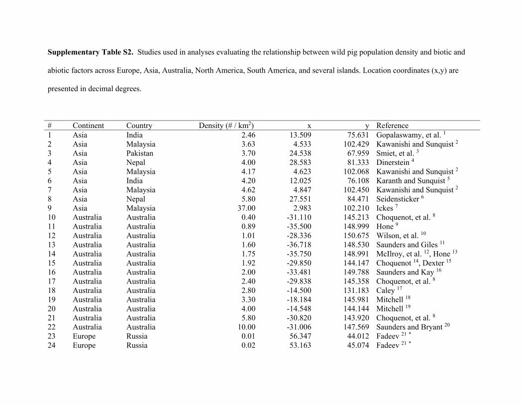
Supplementary Table S2. Studies used in analyses evaluating the relationship between wild pig population density and biotic and

abiotic factors across Europe, Asia, Australia, North America, South America, and several islands. Location coordinates (x,y) are

presented in decimal degrees.

# Continent Country Density (# / km2) x y Reference

1 Asia India 2.46 13.509 75.631 Gopalaswamy, et al. 1

2 Asia Malaysia 3.63 4.533 102.429 Kawanishi and Sunquist 2

3 Asia Pakistan 3.70 24.538 67.959 Smiet, et al. 3

4 Asia Nepal 4.00 28.583 81.333 Dinerstein 4

5 Asia Malaysia 4.17 4.623 102.068 Kawanishi and Sunquist 2

6 Asia India 4.20 12.025 76.108 Karanth and Sunquist 5

7 Asia Malaysia 4.62 4.847 102.450 Kawanishi and Sunquist 2

8 Asia Nepal 5.80 27.551 84.471 Seidensticker 6

9 Asia Malaysia 37.00 2.983 102.210 Ickes 7

10 Australia Australia 0.40 -31.110 145.213 Choquenot, et al. 8

11 Australia Australia 0.89 -35.500 148.999 Hone 9

12 Australia Australia 1.01 -28.336 150.675 Wilson, et al. 10

13 Australia Australia 1.60 -36.718 148.530 Saunders and Giles 11

14 Australia Australia 1.75 -35.750 148.991 McIlroy, et al. 12, Hone 13

15 Australia Australia 1.92 -29.850 144.147 Choquenot 14, Dexter 15

16 Australia Australia 2.00 -33.481 149.788 Saunders and Kay 16

17 Australia Australia 2.40 -29.838 145.358 Choquenot, et al. 8

18 Australia Australia 2.80 -14.500 131.183 Caley 17

19 Australia Australia 3.30 -18.184 145.981 Mitchell 18

20 Australia Australia 4.00 -14.548 144.144 Mitchell 19

21 Australia Australia 5.80 -30.820 143.920 Choquenot, et al. 8

22 Australia Australia 10.00 -31.006 147.569 Saunders and Bryant 20

23 Europe Russia 0.01 56.347 44.012 Fadeev 21 *

24 Europe Russia 0.02 53.163 45.074 Fadeev 21 *

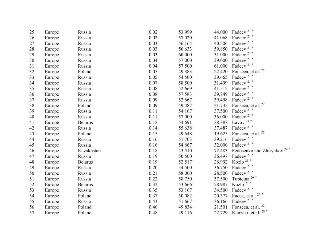
25 Europe Russia 0.02 53.999 44.000 Fadeev 21 *

26 Europe Russia 0.02 57.020 41.068 Fadeev 21 *

27 Europe Russia 0.03 56.164 40.506 Fadeev 21 *

28 Europe Russia 0.03 56.633 59.850 Fadeev 21 *

29 Europe Russia 0.03 60.000 31.000 Fadeev 21 *

30 Europe Russia 0.04 57.000 39.000 Fadeev 21 *

31 Europe Russia 0.04 57.500 61.000 Fadeev 21 *

32 Europe Poland 0.05 49.383 22.420 Fonseca, et al. 22

33 Europe Russia 0.05 54.500 39.665 Fadeev 21 *

34 Europe Russia 0.07 58.500 31.499 Fadeev 21 *

35 Europe Russia 0.08 52.669 41.512 Fadeev 21 *

36 Europe Russia 0.08 57.583 39.749 Fadeev 21 *

37 Europe Russia 0.09 52.667 39.498 Fadeev 21 *

38 Europe Poland 0.09 49.487 21.735 Fonseca, et al. 22

39 Europe Russia 0.11 54.167 37.500 Fadeev 21 *

40 Europe Russia 0.11 57.000 36.000 Fadeev 21 *

41 Europe Belarus 0.12 54.691 28.383 Lavov 23 *

42 Europe Russia 0.14 55.638 37.487 Fadeev 21 *

43 Europe Poland 0.15 49.648 19.625 Fonseca, et al. 22

44 Europe Russia 0.16 51.703 39.216 Fadeev 21 *

45 Europe Russia 0.16 54.667 32.000 Fadeev 21 *

46 Europe Kazakhstan 0.18 43.510 72.483 Fedosenko and Zhiryakov 24 *

47 Europe Russia 0.19 50.500 36.497 Fadeev 21 *

48 Europe Belarus 0.19 52.517 26.992 Kozlo 25 *

49 Europe Russia 0.20 54.500 36.750 Fadeev 21 *

50 Europe Russia 0.21 58.000 28.500 Fadeev 21 *

51 Europe Russia 0.22 58.750 37.500 Tupicina 26 *

52 Europe Belarus 0.32 53.666 28.987 Kozlo 25 *

53 Europe Russia 0.35 53.167 34.500 Fadeev 21 *

54 Europe Poland 0.37 50.082 20.377 Pucek, et al. 27 *

55 Europe Russia 0.43 51.667 36.166 Fadeev 21 *

56 Europe Poland 0.46 49.834 21.501 Fonseca, et al. 22

57 Europe Poland 0.48 49.116 22.729 Kanzaki, et al. 28 *

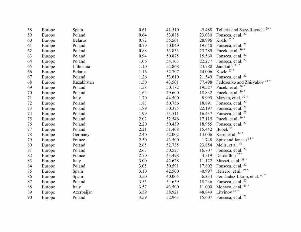
58 Europe Spain 0.61 41.510 -5.488 Tellería and Sáez-Royuela 29 *

59 Europe Poland 0.64 53.885 23.030 Fonseca, et al. 22

60 Europe Belarus 0.72 55.501 28.996 Kozlo 25 *

61 Europe Poland 0.79 50.049 19.640 Fonseca, et al. 22

62 Europe Poland 0.88 53.833 23.289 Pucek, et al. 30 *

63 Europe Poland 0.94 50.875 15.560 Fonseca, et al. 22

64 Europe Poland 1.06 54.103 22.277 Fonseca, et al. 22

65 Europe Lithuania 1.10 54.868 23.780 Janulaitis 31 *

66 Europe Belarus 1.16 52.707 24.006 Kozlo 25 *

67 Europe Poland 1.26 53.610 21.549 Fonseca, et al. 22

68 Europe Kazakhstan 1.50 43.501 77.498 Fedosenko and Zhiryakov 24 *

69 Europe Poland 1.58 50.182 19.527 Pucek, et al. 30 *

70 Europe Poland 1.64 49.600 18.832 Pucek, et al. 30 *

71 Europe Italy 1.70 44.500 8.999 Marsan, et al. 32 *

72 Europe Poland 1.83 50.736 18.891 Fonseca, et al. 22

73 Europe Poland 1.89 50.375 22.197 Fonseca, et al. 22

74 Europe Poland 1.99 53.511 16.437 Fonseca, et al. 22

75 Europe Poland 2.02 52.546 17.115 Pucek, et al. 30 *

76 Europe Poland 2.20 50.459 18.955 Fonseca, et al. 22

77 Europe Poland 2.21 51.408 15.442 Bobek 33

78 Europe Germany 2.40 52.002 13.006 Kern, et al. 34 *

79 Europe France 2.50 43.500 1.748 Spitz and Janeau 35 *

80 Europe Poland 2.65 52.735 23.854 Melis, et al. 36

81 Europe Poland 2.67 50.527 16.707 Fonseca, et al. 22

82 Europe France 2.70 43.498 4.519 Dardaillon 37 *

83 Europe Italy 3.00 42.628 11.122 Massei, et al. 38 *

84 Europe Poland 3.05 50.591 17.802 Fonseca, et al. 22

85 Europe Spain 3.10 42.500 -0.997 Herrero, et al. 39 *

86 Europe Spain 3.50 40.005 -6.334 Fernández-Llario, et al. 40 *

87 Europe Poland 3.55 54.659 18.236 Fonseca, et al. 22

88 Europe Italy 3.57 43.500 11.000 Monaco, et al. 41 *

89 Europe Azerbaijan 3.59 38.921 48.849 Litvinov 42 *

90 Europe Poland 3.59 52.963 15.607 Fonseca, et al. 22

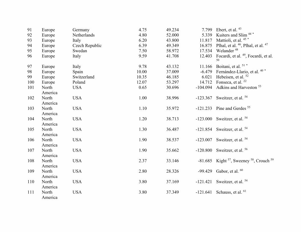
91 Europe Germany 4.75 49.234 7.799 Ebert, et al. 43

92 Europe Netherlands 4.80 52.000 5.339 Kuiters and Slim 44 *

93 Europe Italy 6.20 43.800 11.817 Mattioli, et al. 45 *

94 Europe Czech Republic 6.39 49.349 16.875 Plhal, et al. 46, Plhal, et al. 47

95 Europe Swedan 7.50 58.972 17.534 Welander 48

96 Europe Italy 9.59 41.708 12.403 Focardi, et al. 49, Focardi, et al. 50

97 Europe Italy 9.78 43.132 11.166 Boitani, et al. 51 *

98 Europe Spain 10.00 37.009 -6.479 Fernández-Llario, et al. 40 *

99 Europe Switzerland 10.35 46.185 6.021 Hebeisen, et al. 52

100 Europe Poland 12.07 53.297 14.712 Fonseca, et al. 22

101 North

America

USA 0.65 30.696 -104.094 Adkins and Harveston 53

102 North

America

USA 1.00 38.996 -123.367 Sweitzer, et al. 54

103 North

America

USA 1.10 35.972 -121.233 Pine and Gerdes 55

104 North

America

USA 1.20 38.713 -123.000 Sweitzer, et al. 54

105 North

America

USA 1.30 36.487 -121.854 Sweitzer, et al. 54

106 North

America

USA 1.90 38.537 -123.007 Sweitzer, et al. 54

107 North

America

USA 1.90 35.662 -120.800 Sweitzer, et al. 56

108 North

America

USA 2.37 33.146 -81.685 Kight 57, Sweeney 58, Crouch 59

109 North

America

USA 2.80 28.326 -99.429 Gabor, et al. 60

110 North

America

USA 3.80 37.169 -121.421 Sweitzer, et al. 54

111 North

America

USA 3.80 37.349 -121.641 Schauss, et al. 61

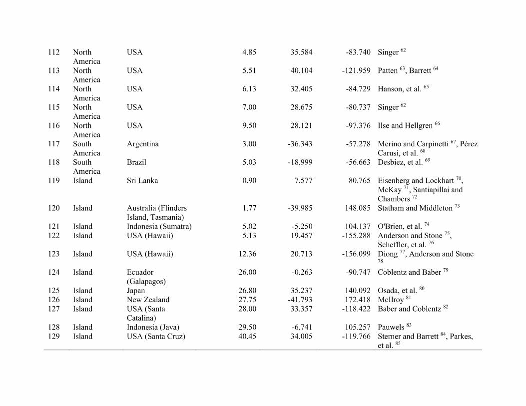
112 North

America

USA 4.85 35.584 -83.740 Singer 62

113 North

America

USA 5.51 40.104 -121.959 Patten 63, Barrett 64

114 North

America

USA 6.13 32.405 -84.729 Hanson, et al. 65

115 North

America

USA 7.00 28.675 -80.737 Singer 62

116 North

America

USA 9.50 28.121 -97.376 Ilse and Hellgren 66

117 South

America

Argentina 3.00 -36.343 -57.278 Merino and Carpinetti 67, Pérez

Carusi, et al. 68

118 South

America

Brazil 5.03 -18.999 -56.663 Desbiez, et al. 69

119 Island Sri Lanka 0.90 7.577 80.765 Eisenberg and Lockhart 70,

McKay 71, Santiapillai and

Chambers 72

120 Island Australia (Flinders

Island, Tasmania)

1.77 -39.985 148.085 Statham and Middleton 73

121 Island Indonesia (Sumatra) 5.02 -5.250 104.137 O'Brien, et al. 74

122 Island USA (Hawaii) 5.13 19.457 -155.288 Anderson and Stone 75,

Scheffler, et al. 76

123 Island USA (Hawaii) 12.36 20.713 -156.099 Diong 77, Anderson and Stone 78

124 Island Ecuador

(Galapagos)

26.00 -0.263 -90.747 Coblentz and Baber 79

125 Island Japan 26.80 35.237 140.092 Osada, et al. 80

126 Island New Zealand 27.75 -41.793 172.418 McIlroy 81

127 Island USA (Santa

Catalina)

28.00 33.357 -118.422 Baber and Coblentz 82

128 Island Indonesia (Java) 29.50 -6.741 105.257 Pauwels 83

129 Island USA (Santa Cruz) 40.45 34.005 -119.766 Sterner and Barrett 84, Parkes,

et al. 85

Notes: * cited in Melis, et al. 36

Literature Cited

1 Gopalaswamy, A., Karanth, K., Kumar, N. & Macdonald, D. Estimating tropical forest ungulate densities from sign surveys

using abundance models of occupancy. Animal Conservation 15, 669-679 (2012).

2 Kawanishi, K. & Sunquist, M. E. Conservation status of tigers in a primary rainforest of Peninsular Malaysia. Biological

Conservation 120, 329-344 (2004).

3 Smiet, A., Fulk, G. & Lathiya, S. Wild boar ecology in Thatta district: a preliminary study. Pak. J. Zool 11, 295-302 (1979).

4 Dinerstein, E. An ecological survey of the Royal Karnali-Bardia Wildlife Reserve, Nepal: Part III: Ungulate populations.

Biological Conservation 18, 5-37 (1980).

5 Karanth, K. U. & Sunquist, M. E. Population structure, density and biomass of large herbivores in the tropical forests of

Nagarahole, India. Journal of Tropical Ecology 8, 21-35 (1992).

6 Seidensticker, J. Ungulate populations in Chitawan valley, Nepal. Biological Conservation 10, 183-210 (1976).

7 Ickes, K. Hyper-abundance of native wild pigs (Sus scrofa) in a lowland Dipterocarp rain forest of peninsular Malaysia

Biotropica 33, 682-690 (2001).

8 Choquenot, D., Lukins, B. & Curran, G. Assessing lamb predation by feral pigs in Australia's semi-arid rangelands. Journal of

Applied Ecology 34, 1445-1454 (1997).

9 Hone, J. Evaluation of methods for ground survey of feral pigs and their sign. Acta Theriologica 33, 451-465 (1988).

10 Wilson, G., Hill, G. & Barnes, A. An aerial survey of feral pigs and emus in southeastern Queensland. Wildlife Research 14,

515-520 (1987).

11 Saunders, G. & Giles, J. Ecological comparison of two wild pig populations in semi-arid and sub-alpine Australia. Journal of

Mountain Ecology 3, 152-155 (1995).

12 McIlroy, J., Braysher, M. & Saunders, G. Effectiveness of a warfarin-poisoning campaign against feral pigs, Sus scrofa, in

Namadgi National Park, ACT. Wildlife Research 16, 195-202 (1989).

13 Hone, J. Feral pigs in Namadgi National Park, Australia: dynamics, impacts and management. Biological Conservation 105,

231-242 (2002).

14 Choquenot, D. The dynamics of feral pig populations in the semi-arid rangelands of eastern Australia Ph.D. thesis, University

of Sydney, (1994).

15 Dexter, N. The behaviour of feral pigs in north-west New South Wales and its implications for the epidemiology of foot and

mouth disease Ph.D. thesis, University of New England, (1996).

16 Saunders, G. & Kay, B. Movements of feral pigs (Sus scrofa) at Sunny Corner, New South Wales. Wildlife Research 18, 49-61

(1991).

17 Caley, P. Population dynamics of feral pigs (Sus scrofa) in a tropical riverine habitat complex. Wildlife Research 20, 625-636

(1993).

18 Mitchell, J. L. Ecology and management of feral pigs (Sus scrofa) in rainforests Ph.D. thesis, James Cook University, (2002).

19 Mitchell, J. The effectiveness of aerial baiting for control of feral pigs (Sus scrofa) in North Queensland. Wildlife Research 25,

297-303 (1998).

20 Saunders, G. & Bryant, H. The evaluation of a feral pig eradication program during a simulated exotic disease outbreak.

Wildlife Research 15, 73-81 (1988).

21 Fadeev, E. Population dynamics of wild boar (Sus scrofa) in European Russia. Zoologicheskii Zhurnal 52, 1214-1219 (1973).

22 Fonseca, C., Kolecki, M., Merta, D. & Bobek, B. Use of line intercept track index and plot sampling for estimating wild boar,

Sus scrofa (Suidae), densities in Poland. Folia Zoologica 56, 389-398 (2007).

23 Lavov, M. Dinamika i regulirovanie chislennosti kabana w Berezinskom zapovednike [Dynamics and regulation of wild boar

abundance in the Berezinskii Reserve]. Zapovedniki Belarusii, 93-98 (1981).

24 Fedosenko, A. & Zhiryakov, V. Ekologiya i povedene kabana v gorakh yuga i yugo-vostoka Kazakhstana.[Ecology and

behaviour of the wild boar in the southern and southeastern Kazakhstan]. Byulleten Moskovskogo Obshchestva Ispytatelei

Prirody, Otdelenie Biologii 89, 36-45 (1984).

25 Kozlo, P. Factors determining the population dynamics of wild boar in Belovezhskyi forest. Zoologicheskii Zhurnal 49, 422-

430 (1970).

26 Tupicina, L. Dinamika chislennosti i razmeshchenie kabana (Sus scrofa) v Darvinskom Zapovednike [Population dynamics

and distribution of wild boar (Sus scrofa) in the Darvinskii Reserve]. Populyacionnye issledovanya zhivotnykh v

zapovednikakh [Populational research in reserves], 128-139 (1988).

27 Pucek, Z., Jędrzejewski, W., Jędrzejewska, B. & Pucek, M. Rodent population dynamics in a primeval deciduous forest

(Białowieża National Park) in relation to weather, seed crop, and predation. Acta Theriologica 38, 199-232 (1993).

28 Kanzaki, N., Perzanowski, K. & Nowosad, M. Factors affecting wild boar (Sus scrofa) population dynamics in Bieszczady,

Poland. Gibier faune sauvage 15, 1171-1178 (1998).

29 Tellería, J. & Sáez-Royuela, C. Ecología de una población ibérica de lobos (Canis lupus). . Acta Vertebrata Doñana 16, 105-

122 (1989).

30 Pucek, Z. et al. Estimates of density and number of ungulates. Polish Ecological Studies 1, 121-135 (1975).

31 Janulaitis, Z. Distribution, abundance and regulation of wild boar population in Lithuania. Acta Zoologica Lituanica 13, 88-88

(2003).

32 Marsan, A., Spano, S. & Tognoni, C. Management attempts of wild boar (Sus scrofa L.): first results and outstanding

researches in northern Apennines (Italy). Journal of Mountain Ecology 3, 219–221 (1995).

33 Bobek, B. Use of a line intercept snow track index and plot sampling for estimating densities of wild boar (Sus scrofa) in

southwestern Poland. Wildlife Biology in Practice 10, 7-16 (2014).

34 Kern, B. et al. Incidence of classical swine fever (CSF) in wild boar in a densely populated area indicating CSF virus

persistence as a mechanism for virus perpetuation. Journal of Veterinary Medicine, Series B 46, 63-68 (1999).

35 Spitz, F. & Janeau, G. Spatial strategies: an attempt to classify daily movements of wild boar. Acta Theriologica 35, 129-149

(1990).

36 Melis, C., Szafrańska, P. A., Jędrzejewska, B. & Bartoń, K. Biogeographical variation in the population density of wild boar

(Sus scrofa) in western Eurasia. Journal of Biogeography 33, 803-811 (2006).

37 Dardaillon, M. Seasonal variations in habitat selection and spatial distribution of wild boar (Sus scrofa) in the Camargue,

Southern France. Behavioural Processes 13, 251-268 (1986).

38 Massei, G., Genov, P., Staines, B. & Gorman, M. Mortality of wild boar, Sus scrofa, in a Mediterranean area in relation to sex

and age. Journal of Zoology 242, 394-400 (1997).

39 Herrero, J., García-Serrano, A. & García-González, R. Wild boar (Sus scrofa L.) hunting in south-western Pyrenees (Spain):

preliminary data. Journal of Mountain Ecology 3, 228-229 (1995).

40 Fernández-Llario, P., Mateos-Quesada, P., Silverio, A. & Santos, P. Habitat effects and shooting techniques on two wild boar

(Sus scrofa) populations in Spain and Portugal. Zeitschrift für Jagdwissenschaft 49, 120-129 (2003).

41 Monaco, A., Pedrotti, L. & Franzetti, B. in 24th Congress of International Union of Game Biologists, Thessaloniki, Greece.

87.

42 Litvinov, V. Vliyanie volka na chislennost kabana v Kyzyl-Agachskom zapovednike [Influence of wolf on wild boar

abundance in the Kyzyl-Agach Reserve]. Kopytnye fauny USSR [Ungulate fauna of the USSR], 173-175 (1980).

43 Ebert, C., Knauer, F., Spielberger, B., Thiele, B. & Hohmann, U. Estimating wild boar Sus scrofa population size using faecal

DNA and capture-recapture modelling. Wildlife Biology 18, 142-152 (2012).

44 Kuiters, A. & Slim, P. Regeneration of mixed deciduous forest in a Dutch forest-heathland, following a reduction of ungulate

densities. Biological Conservation 105, 65-74 (2002).

45 Mattioli, L., Apollonio, M., Mazzarone, V. & Centofanti, E. Wolf food habits and wild ungulate availability in the Foreste

Casentinesi National Park, Italy. Acta Theriologica 40, 387-402 (1995).

46 Plhal, R., Kamler, J., Homolka, M. & Adamec, Z. An assessment of the applicability of photo trapping to estimate wild boar

population density in a forest environment. Folia Zoologica 60, 237-246 (2011).

47 Plhal, R., Kamler, J. & Homolka, M. Faecal pellet group counting as a promising method of wild boar population density

estimation. Acta Theriologica 59, 561-569 (2014).

48 Welander, J. Are wild boars a future threat to the Swedish flora? Journal of Mountain Ecology 3, 165-167 (1995).

49 Focardi, S., Isotti, R., Pelliccioni, E. R. & Iannuzzo, D. The use of distance sampling and mark-resight to estimate the local

density of wildlife populations. Environmetrics 13, 177-186 (2002).

50 Focardi, S., Isotti, R. & Tinelli, A. Line transect estimates of ungulate populations in a Mediterranean forest. The Journal of

Wildlife Management 66, 48-58 (2002).

51 Boitani, L., Trapanese, P. & Mattei, L. Methods of population estimates of a hunted wild boar (Sus scrofa L.) population in

Tuscany (Italy). Journal of Mountain Ecology 3, 204-208 (1995).

52 Hebeisen, C., Fattebert, J., Baubet, E. & Fischer, C. Estimating wild boar (Sus scrofa) abundance and density using capture–

resights in Canton of Geneva, Switzerland. European Journal of Wildlife Research 54, 391-401 (2008).

53 Adkins, R. N. & Harveston, L. A. Demographic and spatial characteristics of feral hogs in the Chihuahuan Desert, Texas.

Human-Wildlife Interactions 1, 152-160 (2007).

54 Sweitzer, R. A., Van Vuren, D., Gardner, I. A., Boyce, W. M. & Waithman, J. D. Estimating sizes of wild pig populations in

the north and central coast regions of California. The Journal of wildlife management 64, 531-543 (2000).

55 Pine, D. & Gerdes, G. Wild pigs in Monterey County, California. California Fish and Game 59, 126-137 (1973).

56 Sweitzer, R. A., Gardner, I. A., Gonzales, B. J., Van Vuren, D. & Boyce, W. M. Population densities and disease surveys of

wild pigs in the coast ranges of central and northern California. Proceedings of 17th Vertebrate Pest Conference, 75-82 (1996).

57 Kight, J. An ecological study of the bobcat, Lynx rufus (Schreber), in west-central South Carolina, University of Georgia,

Athens, GA, USA, (1962).

58 Sweeney, J. Preliminary investigations of a feral hog population on the Savannah River Plant, South Carolina, M.S. Thesis,

University of Georgia, Athens, Georgia, USA, (1970).

59 Crouch, L. C. Movements of and habitat utilization by feral hogs at the Savannah River Plant, South Carolina M.S. Thesis

thesis, Clemson University, Clemson, SC, USA, (1983).

60 Gabor, T. M., Hellgren, E. C., Bussche, R. A. & Silvy, N. J. Demography, sociospatial behaviour and genetics of feral pigs

(Sus scrofa) in a semi-arid environment. Journal of Zoology 247, 311-322 (1999).

61 Schauss, M. E., Coletto, H. J. & Kutilek, M. Population characteristics of wild pigs, Sus scrofa, in eastern Santa Clara County,

California. California Fish and Game 76, 68-77 (1990).

62 Singer, F. J. Wild pig populations in the national parks. Environmental Management 5, 263-270 (1981).

63 Patten, D. C. Feral hogs - boon or burden. Proceedings of the Sixth Vertebrate Pest Conference 6, 210-234 (1974).

64 Barrett, R. H. The feral hog on the Dye Creek Ranch, California. Hilgardia 46, 283-355 (1978).

65 Hanson, L. B. et al. Change-in-ratio density estimator for feral pigs is less biased than closed mark–recapture estimates.

Wildlife Research 35, 695-699 (2008).

66 Ilse, L. M. & Hellgren, E. C. Spatial use and group dynamics of sympatric collared peccaries and feral hogs in southern Texas.

Journal of Mammalogy 76, 993-1002 (1995).

67 Merino, M. L. & Carpinetti, B. N. Feral pig Sus scrofa population estimates in Bahía Samborombón conservation area, Buenos

Aires province, Argentina. Journal of Neotropical Mammal 10, 269-275 (2003).

68 Pérez Carusi, L. C. et al. Relaciones espaciales y numéricas entre venados de las pampas (Ozotoceros bezoarticus celer) y

chanchos cimarrones (Sus scrofa) en el Refugio de Vida Silvestre Bahía Samborombón, Argentina. Ecología Austral 19, 63-71

(2009).

69 Desbiez, A. L. J., Keuroghlian, A., Piovezan, U. & Bodmer, R. E. Invasive species and bushmeat hunting contributing to

wildlife conservation: the case of feral pigs in a Neotropical wetland. Oryx 45, 78-83 (2011).

70 Eisenberg, J. F. & Lockhart, M. An ecological reconnaissance of Wilpattu National Park, Ceylon. (Smithsonian Institution

Press Washington DC, USA, 1972).

71 McKay, G. M. Behavior and ecology of the Asiatic elephant in southeastern Ceylon. (Smithsonian Institution Press

Washington, DC, USA, 1973).

72 Santiapillai, C. & Chambers, M. Aspects of the Population Dynamics of the Wild Pig (Sus scrofa Linnaeus, 1758) in the

Ruhuna National Park. Spixiana 3, 239-250 (1980).

73 Statham, M. & Middleton, M. in Papers and proceedings of the Royal Society of Tasmania. 121-124.

74 O'Brien, T. G., Kinnaird, M. F. & Wibisono, H. T. Crouching tigers, hidden prey: Sumatran tiger and prey populations in a

tropical forest landscape. Animal Conservation 6, 131-139 (2003).

75 Anderson, S. J. & Stone, C. P. Indexing sizes of feral pig populations in a variety of Hawaiian natural areas. Transactions of

the Western Section of the Wildlife Society 30, 26-39 (1994).

76 Scheffler, P. Y., Pratt, L. W., Foote, D. & Magnacca, K. N. A preliminary study of effects of feral pig density on native

Hawaiian montane rainforest vegetation. Technical Report 182 (2012).

77 Diong, C. H. Population biology and management of the feral pig (Sus scrofa L.) in Kipahulu Valley, Maui Ph.D. Thesis

thesis, (1982).

78 Anderson, S. J. & Stone, C. P. Snaring to control feral pigs Sus scrofa in a remote Hawaiian rain forest. Biological

Conservation 63, 195-201 (1993).

79 Coblentz, B. & Baber, D. Biology and control of feral pigs on Isla Santiago, Galapagos, Ecuador. Journal of Applied Ecology

24, 403-418 (1987).

80 Osada, Y., Kuriyama, T., Asada, M., Yokomizo, H. & Miyashita, T. Exploring the drivers of wildlife population dynamics

from insufficient data by Bayesian model averaging. Population Ecology 57, 485-493 (2015).

81 McIlroy, J. Aspects of the ecology of feral pigs (Sus scrofa) in the Murchison area, New Zealand. New Zealand Journal of

Ecology 12, 11-22 (1989).

82 Baber, D. W. & Coblentz, B. E. Density, home range, habitat use, and reproduction in feral pigs on Santa Catalina Island.

Journal of Mammalogy 67, 512-525 (1986).

83 Pauwels, W. Study of Sus scrofa vittatus, its ecology and behavior in Ujung Kulon Nature Reserve, Java, Indonesia, (1980).

84 Sterner, J. D. & Barrett, R. H. Removing feral pigs from Santa Cruz Island, California. Transactions of the Western Section of

the Wildlife Society 27, 47-53 (1991).

85 Parkes, J. P. et al. Rapid eradication of feral pigs (Sus scrofa) from Santa Cruz Island, California. Biological Conservation 143,

634-641 (2010).

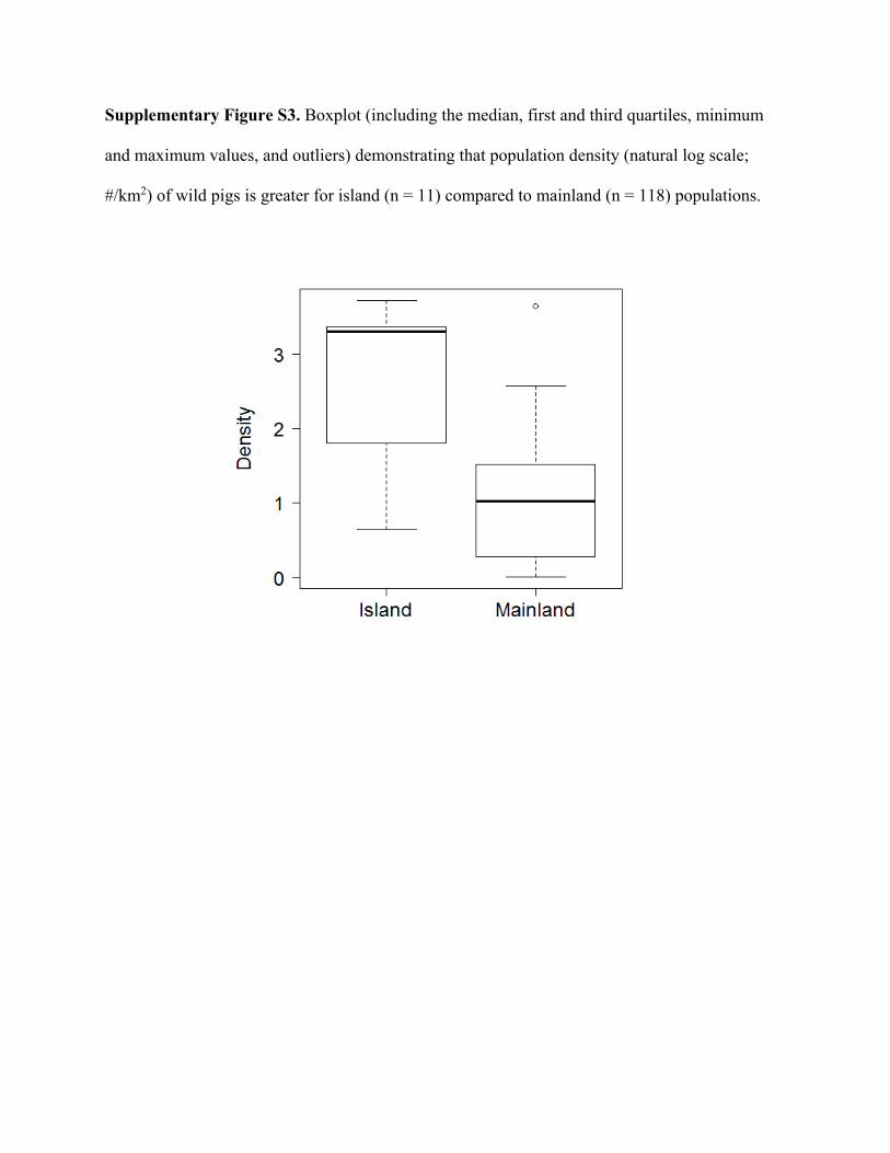
Supplementary Figure S3. Boxplot (including the median, first and third quartiles, minimum

and maximum values, and outliers) demonstrating that population density (natural log scale;

#/km2) of wild pigs is greater for island (n = 11) compared to mainland (n = 118) populations.

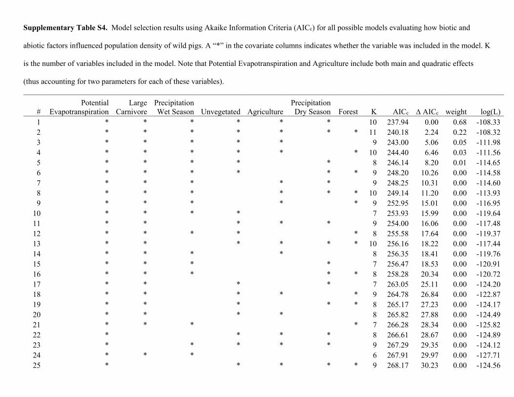
Supplementary Table S4. Model selection results using Akaike Information Criteria (AICc) for all possible models evaluating how biotic and

abiotic factors influenced population density of wild pigs. A “*” in the covariate columns indicates whether the variable was included in the model. K

is the number of variables included in the model. Note that Potential Evapotranspiration and Agriculture include both main and quadratic effects

(thus accounting for two parameters for each of these variables).

#

Potential

Evapotranspiration

Large

Carnivore

Precipitation

Wet Season Unvegetated Agriculture

Precipitation

Dry Season Forest K AICc AICc weight log(L)

1 * * * * * *

10 237.94 0.00 0.68 -108.33

2 * * * * * * * 11 240.18 2.24 0.22 -108.32

3 * * * * *

9 243.00 5.06 0.05 -111.98

4 * * * * *

* 10 244.40 6.46 0.03 -111.56

5 * * * *

*

8 246.14 8.20 0.01 -114.65

6 * * * *

* * 9 248.20 10.26 0.00 -114.58

7 * * *

* *

9 248.25 10.31 0.00 -114.60

8 * * *

* * * 10 249.14 11.20 0.00 -113.93

9 * * *

*

* 9 252.95 15.01 0.00 -116.95

10 * * * *

7 253.93 15.99 0.00 -119.64

11 * *

* * *

9 254.00 16.06 0.00 -117.48

12 * * * *

* 8 255.58 17.64 0.00 -119.37

13 * *

* * * * 10 256.16 18.22 0.00 -117.44

14 * * *

*

8 256.35 18.41 0.00 -119.76

15 * * *

*

7 256.47 18.53 0.00 -120.91

16 * * *

* * 8 258.28 20.34 0.00 -120.72

17 * *

*

*

7 263.05 25.11 0.00 -124.20

18 * *

* *

* 9 264.78 26.84 0.00 -122.87

19 * *

*

* * 8 265.17 27.23 0.00 -124.17

20 * *

* *

8 265.82 27.88 0.00 -124.49

21 * * *

* 7 266.28 28.34 0.00 -125.82

22 *

* * *

8 266.61 28.67 0.00 -124.89

23 *

* * * *

9 267.29 29.35 0.00 -124.12

24 * * *

6 267.91 29.97 0.00 -127.71

25 *

* * * * 9 268.17 30.23 0.00 -124.56

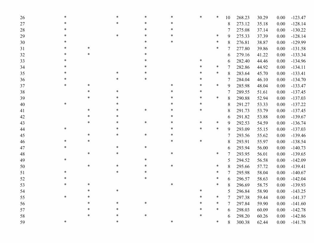
26 *

* * * * * 10 268.23 30.29 0.00 -123.47

27 *

* * *

8 273.12 35.18 0.00 -128.14

28 *

* *

7 275.08 37.14 0.00 -130.22

29 *

* * *

* 9 275.33 37.39 0.00 -128.14

30 *

* *

* 8 276.81 38.87 0.00 -129.99

31 * *

*

* 7 277.80 39.86 0.00 -131.58

32 * *

*

6 279.16 41.22 0.00 -133.34

33 *

*

*

6 282.40 44.46 0.00 -134.96

34 *

*

* * 7 282.86 44.92 0.00 -134.11

35 *

* *

* * 8 283.64 45.70 0.00 -133.41

36 *

* *

*

7 284.04 46.10 0.00 -134.70

37 * *

* * * 9 285.98 48.04 0.00 -133.47

38

* *

* *

7 289.55 51.61 0.00 -137.45

39

* *

* * * 8 290.88 52.94 0.00 -137.03

40 *

*

* *

8 291.27 53.33 0.00 -137.22

41

* * * * *

8 291.73 53.79 0.00 -137.45

42

* *

*

6 291.82 53.88 0.00 -139.67

43

* * * * * * 9 292.53 54.59 0.00 -136.74

44 *

*

* * * 9 293.09 55.15 0.00 -137.03

45

* * * *

7 293.56 55.62 0.00 -139.46

46 * *

* *

8 293.91 55.97 0.00 -138.54

47 *

* *

6 293.94 56.00 0.00 -140.73

48

* *

*

* 7 293.95 56.01 0.00 -139.65

49 *

*

5 294.52 56.58 0.00 -142.09

50

* * * *

* 8 295.66 57.72 0.00 -139.41

51 *

* *

* 7 295.98 58.04 0.00 -140.67

52 *

*

* 6 296.57 58.63 0.00 -142.04

53 * *

*

* 8 296.69 58.75 0.00 -139.93

54

* *

*

5 296.84 58.90 0.00 -143.25

55 * *

* * 7 297.38 59.44 0.00 -141.37

56

* * *

* * 7 297.84 59.90 0.00 -141.60

57

* *

* * 6 298.03 60.09 0.00 -142.78

58

* * *

*

6 298.20 60.26 0.00 -142.86

59 *

*

*

* 8 300.38 62.44 0.00 -141.78

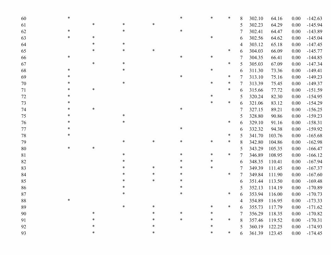
60 *

* * * 8 302.10 64.16 0.00 -142.63

61

* * *

5 302.23 64.29 0.00 -145.94

62 *

*

*

7 302.41 64.47 0.00 -143.89

63 * *

*

6 302.56 64.62 0.00 -145.04

64

* *

4 303.12 65.18 0.00 -147.45

65

* * *

* 6 304.03 66.09 0.00 -145.77

66 *

* *

7 304.35 66.41 0.00 -144.85

67

* *

* 5 305.03 67.09 0.00 -147.34

68 *

*

*

6 311.30 73.36 0.00 -149.41

69 *

*

* 7 313.10 75.16 0.00 -149.23

70 *

*

* * 7 313.39 75.45 0.00 -149.37

71 * *

* 6 315.66 77.72 0.00 -151.59

72 *

*

5 320.24 82.30 0.00 -154.95

73 *

* * 6 321.06 83.12 0.00 -154.29

74 * *

*

7 327.15 89.21 0.00 -156.25

75 *

*

5 328.80 90.86 0.00 -159.23

76 *

*

* 6 329.10 91.16 0.00 -158.31

77 *

*

6 332.32 94.38 0.00 -159.92

78 *

* 5 341.70 103.76 0.00 -165.68

79

* * * * * 8 342.80 104.86 0.00 -162.98

80 * *

5 343.29 105.35 0.00 -166.47

81

*

* * * 7 346.89 108.95 0.00 -166.12

82

*

* *

6 348.35 110.41 0.00 -167.94

83

* * * *

7 349.39 111.45 0.00 -167.37

84

* * *

* 7 349.84 111.90 0.00 -167.60

85

* * *

6 351.44 113.50 0.00 -169.48

86

*

*

5 352.13 114.19 0.00 -170.89

87

*

*

* 6 353.94 116.00 0.00 -170.73

88 *

4 354.89 116.95 0.00 -173.33

89

* *

* * 6 355.73 117.79 0.00 -171.62

90

*

* * *

7 356.29 118.35 0.00 -170.82

91

*

* * * * 8 357.46 119.52 0.00 -170.31

92

*

*

*

5 360.19 122.25 0.00 -174.93

93

*

*

* * 6 361.39 123.45 0.00 -174.45

94

*

* *

6 364.46 126.52 0.00 -175.99

95

*

* * * 7 365.36 127.42 0.00 -175.36

96

* *

*

5 366.68 128.74 0.00 -178.17

97

*

* * 5 367.68 129.74 0.00 -178.67

98

* *

* 5 368.27 130.33 0.00 -178.96

99

* * * * 7 368.31 130.37 0.00 -176.83

100

*

* *

6 368.90 130.96 0.00 -178.21

101

*

*

4 370.36 132.42 0.00 -181.07

102

*

* *

* 7 370.64 132.70 0.00 -178.00

103

* * *

6 370.68 132.74 0.00 -179.10

104

* *

4 372.16 134.22 0.00 -181.97

105

*

*

4 372.62 134.68 0.00 -182.20

106

*

* * 5 373.43 135.49 0.00 -181.54

107

*

*

4 376.60 138.66 0.00 -184.19

108

*

* * 5 376.95 139.01 0.00 -183.30

109

* *

5 377.07 139.13 0.00 -183.36

110

*

*

* 5 378.16 140.22 0.00 -183.91

111

* * * 6 379.21 141.27 0.00 -183.36

112

*

*

* 6 379.42 141.48 0.00 -183.47

113

* *

5 379.92 141.98 0.00 -184.79

114

*

*

4 381.25 143.31 0.00 -186.51

115

* *

* 6 381.81 143.87 0.00 -184.66

116

*

3 382.24 144.30 0.00 -188.05

117

*

* 4 384.24 146.30 0.00 -188.00

118

*

*

5 392.46 154.52 0.00 -191.06

119

*

3 393.53 155.59 0.00 -193.70

120

*

* 5 393.80 155.86 0.00 -191.73

121

*

3 393.98 156.04 0.00 -193.92

122

*

* 4 395.38 157.44 0.00 -193.58

123

*

* 4 395.45 157.51 0.00 -193.61

124

* * 4 395.52 157.58 0.00 -193.64

125

*

4 399.33 161.39 0.00 -195.55

126

*

3 413.34 175.40 0.00 -203.60

127

* 3 421.30 183.36 0.00 -207.58

128 2 428.33 190.39 0.00 -212.13

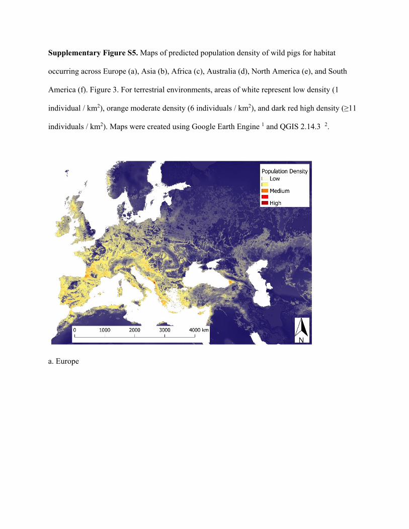
Supplementary Figure S5. Maps of predicted population density of wild pigs for habitat

occurring across Europe (a), Asia (b), Africa (c), Australia (d), North America (e), and South

America (f). Figure 3. For terrestrial environments, areas of white represent low density (1

individual / km2), orange moderate density (6 individuals / km2), and dark red high density (≥11

individuals / km2). Maps were created using Google Earth Engine 1 and QGIS 2.14.3 2.

a. Europe

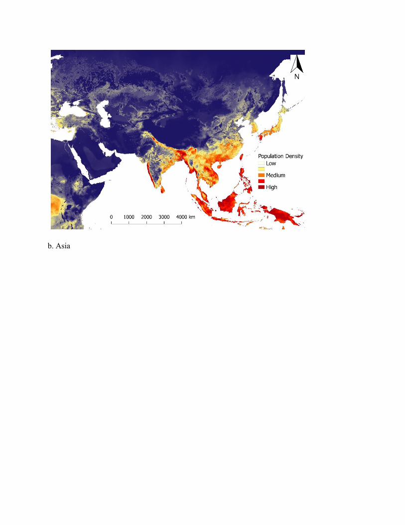
b. Asia

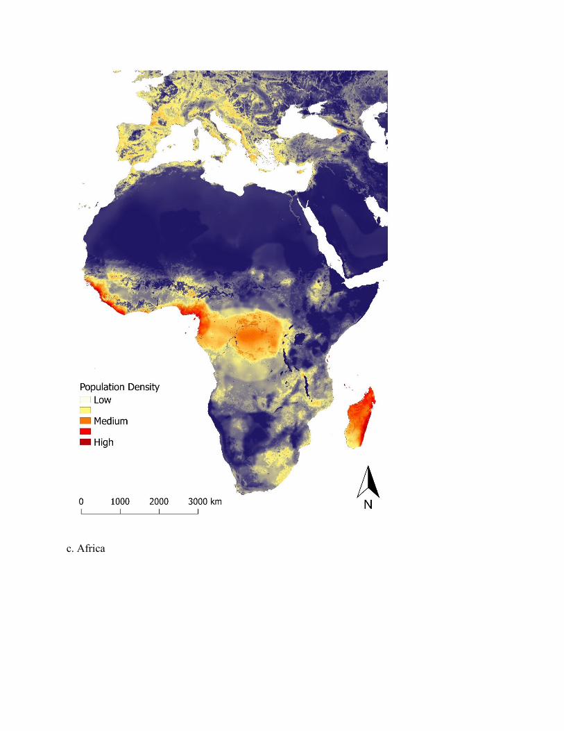
c. Africa

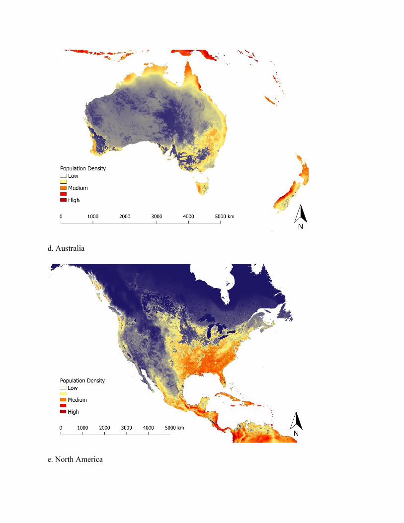
d. Australia

e. North America

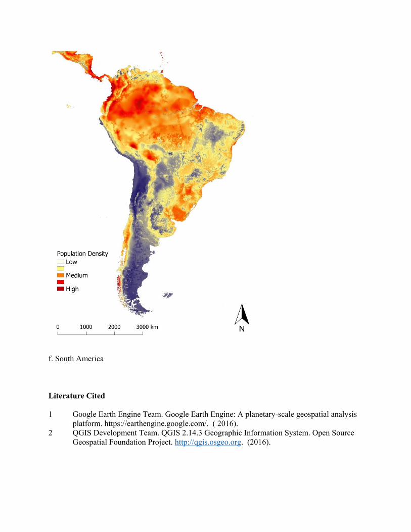
f. South America

Literature Cited

1 Google Earth Engine Team. Google Earth Engine: A planetary-scale geospatial analysis

platform. https://earthengine.google.com/. ( 2016).

2 QGIS Development Team. QGIS 2.14.3 Geographic Information System. Open Source

Geospatial Foundation Project. http://qgis.osgeo.org. (2016).