bk1 - eceweb1.rutgers.edueceweb1.rutgers.edu/~orfanidi/ewa/ch23.pdf · 23 Array Design Methods 23.1 Array Design Methods As we mentioned in Sec. 22.4, the array design problem is

23Array Design Methods

23.1 Array Design Methods

As we mentioned in Sec. 22.4, the array design problem is essentially equivalent to theproblem of designing FIR digital filters in DSP. Following this equivalence, we discussseveral array design methods, such as:

1. Schelkunoff’s zero placement method2. Fourier series method with windowing3. Woodward-Lawson frequency-sampling design4. Narrow-beam low-sidelobe design methods5. Multi-beam array design

Next, we establish some common notation. One-dimensional equally-spaced arraysare usually considered symmetrically with respect to the origin of the array axis. Thisrequires a slight redefinition of the array factor in the case of even number of arrayelements. Consider an array ofN elements at locations xm along the x-axis with elementspacing d. The array factor will be:

A(φ)=∑mamejkxxm =

∑mamejkxm cosφ

where kx = k cosφ (for polar angle θ = π/2.) If N is odd, say N = 2M + 1, we candefine the element locations xm symmetrically as:

xm =md, m = 0,±1,±2, . . . ,±MThis was the definition we used in Sec. 22.4. The array factor can be written then as

a discrete-space Fourier transform or as a spatial z-transform:

A(ψ) =M∑

m=−Mamejmψ = a0 +

M∑m=1

[amejmψ + a−me−jmψ

]

A(z) =M∑

m=−Mamzm = a0 +

M∑m=1

[amzm + a−mz−m

] (23.1.1)

1120 23. Array Design Methods

where ψ = kxd = kd cosφ and z = ejψ. On the other hand, if N is even, say N = 2M,in order to have symmetry with respect to the origin, we must place the elements at thehalf-integer locations:

x±m = ±(md− d

2

) = ±(m− 1

2

)d, m = 1,2, . . . ,M

The array factor will be now:

A(ψ) =M∑m=1

[amej(m−1/2)ψ + a−me−j(m−1/2)ψ

]

A(z) =M∑m=1

[amzm−1/2 + a−mz−(m−1/2)

] (23.1.2)

In particular, if the array weights am are symmetric with respect to the origin, am =a−m, as they are in most design methods, then the array factor can be simplified intothe cosine forms:

A(ψ)= a0 + 2M∑m=1

am cos(mψ), (N = 2M + 1)

A(ψ)= 2M∑m=1

am cos((m− 1/2)ψ)

), (N = 2M)

(23.1.3)

In both the odd and even cases, Eqs. (23.1.1) and (23.1.2) can be expressed as theleft-shifted version of a right-sided z-transform:

A(z)= z−(N−1)/2A(z)= z−(N−1)/2N−1∑n=0

anzn (23.1.4)

where a = [a0, a1, . . . , aN−1] is the vector of array weights reindexed to be right-sided.In terms of the original symmetric weights, we have:

[a0, a1, . . . , aN−1]= [a−M, . . . , a−1, a0, a1, . . . , aM], (N = 2M + 1)

[a0, a1, . . . , aN−1]= [a−M, . . . , a−1, a1, . . . , aM], (N = 2M)(23.1.5)

In time-domain DSP, a factor of z represents a time-advance or left shift. But in thespatial domain, a left shift is represented by z−1 because of the opposite sign conventionin the definition of the z-transform. Thus, the factor z−(N−1)/2 represents a left shift bya distance (N − 1)d/2, which places the middle of the right-sided array at the origin.For instance, see Examples 22.3.1 and 22.3.2.

The corresponding array factors in ψ-space are related in a similar fashion. Settingz = ejψ, we have:

A(ψ)= e−jψ(N−1)/2A(ψ)= e−jψ(N−1)/2N−1∑n=0

anejnψ (23.1.6)

23.1. Array Design Methods 1121

Working with A(ψ) is more convenient for programming purposes, as it can becomputed by an ordinary DTFT routine, such as that in Ref. [49], A(ψ)= dtft(a,−ψ).The phase factor e−jψ(N−1)/2 does not affect the power gain of the array; indeed, wehave |A(ψ)|2 = |A(ψ)|2 = |dtft(a,−ψ)|2.

Some differences arise also for steered array factors. Given a steering phase ψ0 =kd cosφ0, we define the steered array factor as A′(ψ)= A(ψ−ψ0). Then, we have:

A′(ψ)= A(ψ−ψ0)= e−j(ψ−ψ0)(N−1)/2A(ψ−ψ0)= e−jψ(N−1)/2A′(ψ)

It follows that the steered version of A(ψ) will be:

A′(ψ)= ejψ0(N−1)/2A(ψ−ψ0) (23.1.7)

which implies for the weights:

a′n = ane−jψ0(n−(N−1)/2) , n = 0,1, . . . ,N − 1 (23.1.8)

This simply means that the progressive phase is measured with respect to the middleof the array. Again, the common phase factor ejψ0(N−1)/2 is usually unimportant. Onecase where it is important is the case of multiple beams steered towards different angles;these are discussed in Sec. 23.14. In the symmetric notation, the steered weights are asfollows:

a′m = ame−jmψ0 , m = 0,±1,±2, . . . ,±M, (N = 2M + 1)

a′±m = a±me∓j(m−1/2)ψ0 , m = 1,2, . . . ,M, (N = 2M)(23.1.9)

The MATLAB functions scan and steer perform the desired progressive phasing ofthe weights according to Eq. (23.1.8). Their usage is as follows:

ascan = scan(a, psi0); % scan array with given scanning phase ψ0

asteer = steer(d, a, ph0); % steer array towards given angle φ0

Example 23.1.1: For the cases N = 7 and N = 6, we have M = 3. The symmetric and right-sided array weights will be related as follows:

a = [a0, a1, a2, a3, a4, a5, a6]= [a−3, a−2, a−1, a0, a1, a2, a3]

a = [a0, a1, a2, a3, a4, a5]= [a−3, a−2, a−1, a1, a2, a3]

For N = 7 we have (N − 1)/2 = 3, and for N = 6, (N − 1)/2 = 5/2. Thus, the arraylocations along the x-axis will be:

xm ={−3d, −2d, −d, 0, d, 2d, 3d

}

xm ={−5

2d, −3

2d, −1

2d,

1

2d,

3

2d,

5

2d}

Eq. (23.1.4) reads as follows in the two cases:

A(z) = a−3z−3 + a−2z−2 + a−1z−1 + a0 + a1z+ a2z2 + a3z3

= z−3[a−3 + a−2z+ a−1z2 + a0z3 + a1z4 + a2z5 + a3z6

] = z−3A(z)

A(z) = a−3z−5/2 + a−2z−3/2 + a−1z−1/2 + a1z1/2 + a2z3/2 + a3z5/2

= z−5/2[a−3 + a−2z+ a−1z2 + a1z3 + a2z4 + a3z5] = z−5/2A(z)


If the arrays are steered, the weights pick up the progressive phases:

[a−3ej3ψ0 , a−2ej2ψ0 , a−1ejψ0 , a0, a1e−jψ0 , a2e−j2ψ0 , a3e−j3ψ0

]= ej3ψ0

[a−3, a−2e−jψ0 , a−1e−2jψ0 , a0e−3jψ0 , a1e−4jψ0 , a2e−j5ψ0 , a3e−j6ψ0

][a−3ej5ψ0/2, a−2ej3ψ0/2, a−1ejψ0/2, a1e−jψ0/2, a2e−j3ψ0/2, a3e−j5ψ0/2

]= ej5ψ0/2

[a−3, a−2e−jψ0 , a−1e−2jψ0 , a1e−3jψ0 , a2e−j4ψ0 , a3e−j5ψ0

]

where ψ0 = kd cosφ0 is the steering phase. ��

Example 23.1.2: The uniform array of Sec. 22.7, was defined as a right-sided array. In thepresent notation, the weights and array factor are:

a = [a0, a1, . . . , aN−1]= 1

N[1,1, . . . ,1], A(z)= 1

NzN − 1

z− 1

Using Eq. (23.1.4), the corresponding symmetric array factor will be:

A(z)= z−(N−1)/2A(z)= z−(N−1)/2 1

NzN − 1

z− 1= 1

NzN/2 − z−N/2z1/2 − z−1/2

Setting z = ejψ, we obtain

A(ψ)=sin(Nψ

2

)

N sin(ψ2

) (23.1.10)

which also follows from Eqs. (22.7.3) and (23.1.6). ��

23.2 Schelkunoff’s Zero Placement Method

The array factor of an N-element array is a polynomial of degree N− 1 and therefore ithas N − 1 zeros:

A(z)=N−1∑n=0

anzn = (z− z1)(z− z2)· · · (z− zN−1)aN−1 (23.2.1)

By proper placement of the zeros on the z-plane, a desired array factor can be de-signed. Schelkunoff’s paper of more than 45 years ago [1243] discusses this and theFourier series methods.

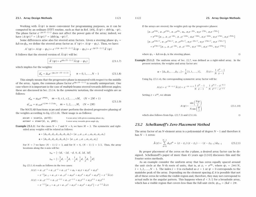
As an example consider the uniform array that has zeros equally spaced aroundthe unit circle at the N-th roots of unity, that is, at zi = ejψi , where ψi = 2πi/N,i = 1,2, . . . ,N − 1. The index i = 0 is excluded as z = 1 or ψ = 0 corresponds to themainlobe peak of the array. Depending on the element spacing d, it is possible that notall of these zeros lie within the visible region and, therefore, they may not correspond toactual nulls in the angular pattern. This happens when d < λ/2 for a broadside array,which has a visible region that covers less than the full unit circle, ψvis = 2kd < 2π.

23.2. Schelkunoff’s Zero Placement Method 1123

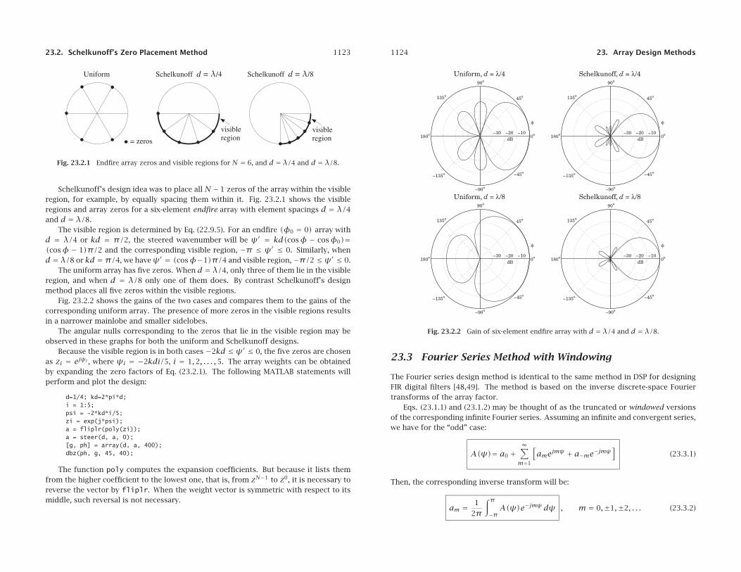
Fig. 23.2.1 Endfire array zeros and visible regions for N = 6, and d = λ/4 and d = λ/8.

Schelkunoff’s design idea was to place all N− 1 zeros of the array within the visibleregion, for example, by equally spacing them within it. Fig. 23.2.1 shows the visibleregions and array zeros for a six-element endfire array with element spacings d = λ/4and d = λ/8.

The visible region is determined by Eq. (22.9.5). For an endfire (φ0 = 0) array withd = λ/4 or kd = π/2, the steered wavenumber will be ψ′ = kd(cosφ − cosφ0)=(cosφ − 1)π/2 and the corresponding visible region, −π ≤ ψ′ ≤ 0. Similarly, whend = λ/8 or kd = π/4, we haveψ′ = (cosφ−1)π/4 and visible region,−π/2 ≤ ψ′ ≤ 0.

The uniform array has five zeros. When d = λ/4, only three of them lie in the visibleregion, and when d = λ/8 only one of them does. By contrast Schelkunoff’s designmethod places all five zeros within the visible regions.

Fig. 23.2.2 shows the gains of the two cases and compares them to the gains of thecorresponding uniform array. The presence of more zeros in the visible regions resultsin a narrower mainlobe and smaller sidelobes.

The angular nulls corresponding to the zeros that lie in the visible region may beobserved in these graphs for both the uniform and Schelkunoff designs.

Because the visible region is in both cases −2kd ≤ ψ′ ≤ 0, the five zeros are chosenas zi = ejψi , where ψi = −2kdi/5, i = 1,2, . . . ,5. The array weights can be obtainedby expanding the zero factors of Eq. (23.2.1). The following MATLAB statements willperform and plot the design:

d=1/4; kd=2*pi*d;i = 1:5;psi = -2*kd*i/5;zi = exp(j*psi);a = fliplr(poly(zi));a = steer(d, a, 0);[g, ph] = array(d, a, 400);dbz(ph, g, 45, 40);

The function poly computes the expansion coefficients. But because it lists themfrom the higher coefficient to the lowest one, that is, from zN−1 to z0, it is necessary toreverse the vector by fliplr. When the weight vector is symmetric with respect to itsmiddle, such reversal is not necessary.


90o

−90o

0o180o

φ

45o

−45o

135o

−135o

−10−20−30dB

Uniform, d = λ/4 90o

−90o

0o180o

φ

45o

−45o

135o

−135o

−10−20−30dB

Schelkunoff, d = λ/4

90o

−90o

0o180o

φ

45o

−45o

135o

−135o

−10−20−30dB

Uniform, d = λ/8 90o

−90o

0o180o

φ

45o

−45o

135o

−135o

−10−20−30dB

Schelkunoff, d = λ/8

Fig. 23.2.2 Gain of six-element endfire array with d = λ/4 and d = λ/8.

23.3 Fourier Series Method with Windowing

The Fourier series design method is identical to the same method in DSP for designingFIR digital filters [48,49]. The method is based on the inverse discrete-space Fouriertransforms of the array factor.

Eqs. (23.1.1) and (23.1.2) may be thought of as the truncated or windowed versionsof the corresponding infinite Fourier series. Assuming an infinite and convergent series,we have for the “odd” case:

A(ψ)= a0 +∞∑m=1

[amejmψ + a−me−jmψ

](23.3.1)

Then, the corresponding inverse transform will be:

am = 1

2π

∫ π−πA(ψ)e−jmψ dψ , m = 0,±1,±2, . . . (23.3.2)

23.4. Sector Beam Array Design 1125

Similarly, in the “even” case we have:

A(ψ)=∞∑m=1

[amej(m−1/2)ψ + a−me−j(m−1/2)ψ

](23.3.3)

with inverse transform:

a±m = 1

2π

∫ π−πA(ψ)e∓j(m−1/2)ψ dψ , m = 1,2, . . . (23.3.4)

In general, a desired array factor requires an infinite number of coefficients am to berepresented exactly. Keeping only a finite number of coefficients in the Fourier seriesintroduces unwanted ripples in the desired response, known as the Gibbs phenomenon[48,49]. Such ripples can be minimized using an appropriate window, but at the expenseof wider transition regions.

The Fourier series method may be summarized as follows. Given a desired response,say Ad(ψ), pick an odd or even window length, for example N = 2M+ 1, and calculatethe N ideal weights by evaluating the inverse transform:

ad(m)= 1

2π

∫ π−πAd(ψ)e−jmψ dψ , m = 0,±1, . . . ,±M (23.3.5)

then, the final weights are obtained by windowing with a length-N window w(m):

a(m)= w(m)ad(m), m = 0,±1, . . . ,±M (23.3.6)

This method is convenient only when the required integral (23.3.5) can be done ex-actly, as when Ad(ψ) has a simple shape such as an ideal lowpass filter. For arbitrarilyshaped Ad(ψ) one must evaluate the integrals approximately using an inverse DFTas is done in the Woodward- Lawson frequency-sampling design method discussed inSec. 23.5.

In addition, the method requires thatAd(ψ) be specified over one complete Nyquistinterval, −π ≤ ψ ≤ π, regardless of whether the visible region ψvis = 2kd is more orless than one Nyquist period.

23.4 Sector Beam Array Design

As an example of the Fourier series method, we discuss the design of an array withangular pattern confined into a desired angular sector.

First, we consider the design in ψ-space of an ideal bandpass array factor centeredat wavenumber ψ0 with bandwidth of 2ψb. We will see later how to map these spec-ifications into an actual angular sector. The ideal bandpass response is defined over−π ≤ ψ ≤ π as follows:

ABP(ψ)={

1, ψ0 −ψb ≤ ψ ≤ ψ0 +ψb0, otherwise


For the odd case, the corresponding ideal weights are obtained from Eq. (23.3.2):

aBP(m)= 1

2π

∫ π−πABP(ψ)e−jmψ dψ = 1

2π

∫ ψ0+ψb

ψ0−ψb1 · e−jmψ dψ

which gives:

aBP(m)= e−jmψ0sin(ψbm)πm

, m = 0,±1,±2, . . . (23.4.1)

This problem is equivalent to designing an ideal lowpass response with cutoff fre-quency ψb and then translating it by ABP(ψ)= ALP(ψ′)= ALP(ψ −ψ0), where ψ′ =ψ−ψ0. The lowpass response is defined as:

ALP(ψ′)={

1, −ψb ≤ ψ′ ≤ ψb0, otherwise

and its ideal weights are:

aLP(m)= 1

2π

∫ π−πALP(ψ′)e−jmψ

′dψ′ = 1

2π

∫ ψb−ψb

1 · e−jmψ′ dψ′ = sin(ψbm)πm

Thus, as expected, the ideal weights for the bandpass and lowpass designs are relatedby a scanning phase: aBP(m)= e−jmψ0aLP(m).

A more realistic design of the bandpass response is to prescribe “brickwall” specifi-cations, that is, defining a passband range over which the response is essentially flat anda stopband range over which the response is essentially zero. These ranges are definedby the bandedge frequencies ψp and ψs, such that the passband is |ψ−ψ0| ≤ ψp andthe stopband |ψ−ψ0| ≥ ψs. The specifications of the equivalent lowpass response areshown in Fig. 23.4.1.

Fig. 23.4.1 Specifications of equivalent lowpass response.

Over the stopband, the attenuation is required to be greater than a minimum value,say A dB. The attenuation over the passband need not be specified, because the windowmethod always results in extremely flat passbands for reasonable values of A, e.g., forA > 35 dB. Indeed, the maximum passband attenuation is related to A by the approxi-mate formula Apass = 17.4δ dB, where δ = 10−A/20 (see Ref. [49].)

Most windows do not allow a user-defined choice for the stopband attenuation. Forexample, the Hamming window has A = 54 dB and the rectangular window A = 21 dB.

23.4. Sector Beam Array Design 1127

The Kaiser window is the best and simplest of a small class of windows that allow avariable choice for A.

Thus, the design specifications are the quantities {ψp,ψs,A}. Alternatively, we cantake them to be {ψp,Δψ,A}, where Δψ = ψs −ψp is the transition width. We preferthe latter choice. The design steps for the bandpass response using the Kaiser windoware summarized below:

1. From the stopband attenuation A, calculate the so-called D-factor of the window(similar to the broadening factor):

D =⎧⎪⎨⎪⎩A− 7.95

14.36, if A > 21

0.922, if A ≤ 21(23.4.2)

and the window’s shape parameter α:

α =

⎧⎪⎪⎨⎪⎪⎩

0.1102(A− 8.7), if A≥ 50

0.5842(A− 21)0.4+0.07886(A− 21), if 21<A< 50

0, if A ≤ 21

(23.4.3)

2. From the transition width Δψ, calculate the length of the window by choosing thesmallest odd integer N = 2M + 1 that satisfies:

Δψ = 2πDN − 1

(23.4.4)

Alternatively, if N is given, calculate the transition width Δψ.

3. Calculate the samples of the Kaiser window:

w(m)= I0(α√

1−m2/M2)

I0(α), m = 0,±1, . . . ,±M (23.4.5)

where I0(x) is the modified Bessel function of first kind and zeroth order.

4. Calculate the ideal cutoff frequency ψb by taking it to be at the middle betweenthe passband and stopband frequencies:

ψb = 1

2(ψp +ψs)= ψp + 1

2Δψ (23.4.6)

5. Calculate the final windowed array weights from a(m)= w(m)aBP(m):

a(m)= w(m)e−jmψ0sin(ψbm)πm

, m = 0,±1, . . . ,±M (23.4.7)


Next, we use the above bandpass design inψ-space to design an array with an angularsector response inφ-space. The ideal array will have a pattern that is uniformly flat overan angular sector [φ1,φ2]:

A(φ)={

1, φ1 ≤ φ ≤ φ2

0, otherwise

Alternatively, we can define the sector by means of its center angle and its width,φc = (φ1 +φ2)/2 and φb = φ2 −φ1. Thus, we have the equivalent definitions of theangular sector:

φc = 1

2(φ1 +φ2)

φb = φ2 −φ1

�φ1 = φc − 1

2φb

φ2 = φc + 1

2φb

(23.4.8)

For a practical design, we may take [φ1,φ2] to represent the passband of the re-sponse and assume an angular stopband with attenuation of at least A dB that beginsafter a small angular transition width Δφ on either side of the passband.

In filter design, the stopband attenuation and the transition width are used to deter-mine the window length N. But in the array problem, because we are usually limited inthe number N of available array elements, we must assume that N is given and deter-mine the transition width Δφ from A and N.

Thus, our design specifications are the quantities {φ1,φ2,N,A}, or alternatively,{φc,φb,N,A}. These specifications must be mapped into equivalent ones in ψ-spaceusing the steered wavenumber ψ′ = kd(cosφ− cosφ0).

We require that the angular passband [φ1,φ2] be mapped onto the lowpass pass-band [−ψp,ψp] in ψ′-space. Thus, we have the conditions:

ψp = kd cosφ1 −ψ0

−ψp = kd cosφ2 −ψ0

They may be solved for ψp and ψ0 as follows:

ψp = 1

2kd(cosφ1 − cosφ2)

ψ0 = 1

2kd(cosφ1 + cosφ2)

(23.4.9)

Using Eq. (23.4.8) and some trigonometry, we have equivalently:

ψp = kd sin(φc)sin(φb

2

)

ψ0 = kd cos(φc)cos(φb

2

) (23.4.10)

Setting ψ0 = kd cosφ0, we find the effective steering angle φ0:

cosφ0 = cos(φc)cos(φb

2

) ⇒ φ0 = acos(cos(φc)cos(φb/2)

)(23.4.11)

23.5. Woodward-Lawson Frequency-Sampling Design 1129

Note that φ0 is not equal to φc, except for very narrow widths φb.The design procedure is then completed as follows. Given the attenuation A, we

calculate the window parameters D,α from Eqs. (23.4.2) and (23.4.3). Since N is given,we calculate the transition width Δψ directly from Eq. (23.4.4). Then, the ideal lowpassfrequency ψb is calculated from Eq. (23.4.6), that is,

ψb = ψp + 1

2Δψ = kd sin(φc)sin

(φb2

)+ πDN − 1

(23.4.12)

Finally, the array weights are obtained from Eq. (23.4.7). The transition width Δφcan be approximated by linearizing ψ = kd cosφ around φ1, or around φ2, or aroundφc. We prefer the latter choice, giving:

Δφ = Δψkd sinφc

= 2πDkd(N − 1)sinφc

(23.4.13)

The design method can be extended to the case of evenN = 2M. The integral (23.3.4)can still be done exactly. The Kaiser window expression (23.4.5) remains the same form = ±1,±2, . . . ,±M. We note the symmetry w(−m)= w(m). After windowing andscanning with ψ0, we get the final designed weights:

a(±m)= w(m)e∓j(m−1/2)ψ0sin(ψb(m− 1/2)

)π(m− 1/2)

, m = 1,2, . . . ,M (23.4.14)

The MATLAB function sector implements the above design steps for either even orodd N. Its usage is as follows:

[a, dph] = sector(d, ph1, ph2, N, A); % A=stopband attenuation in dB

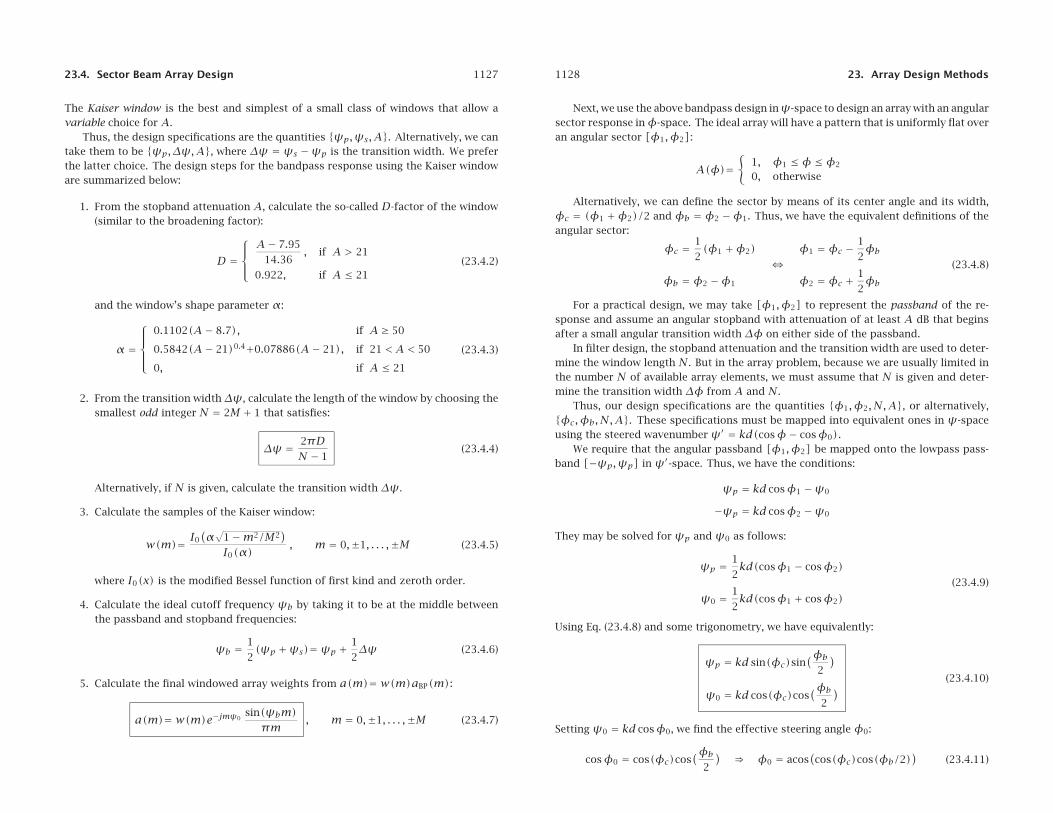
Fig. 23.4.2 shows four design examples having sector [φ1,φ2]= [45o,75o], or cen-ter φc = 60o and width φb = 30o. The number of array elements was N = 21 andN = 41, with half-wavelength spacing d = λ/2. The stopband attenuations wereA = 20and A = 40 dB. The two cases with A = 20 dB are equivalent to using the rectangularwindow. They have visible Gibbs ripples in their passband. Some typical MATLAB codefor generating these graphs is as follows:

d=0.5; ph1=45; ph2=75; N=21; A=20;[a, dph] = sector(d, ph1, ph2, N, A);[g, ph] = array(d, a, 400);dbz(ph,g, 30, 80);addray(ph1, ’--’); addray(ph2, ’--’);

The basic design tradeoff is betweenN andA and is captured by Eq. (23.4.4). BecauseD is linearly increasing with A, the transition width will increase with A and decreasewith N. As A increases, the passband exhibits no Gibbs ripples but at the expense oflarger transition width.

23.5 Woodward-Lawson Frequency-Sampling Design

As we mentioned earlier, the Fourier series method is feasible only when the inversetransform integrals (23.3.2) and (23.3.4) can be done exactly. If not, we may use the


90o

−90o

0o180o

φ

60o

−60o

30o

−30o

120o

−120o

150o

−150o

−20−40−60dB

N = 21, A = 20 dB 90o

−90o

0o180o

φ

60o

−60o

30o

−30o

120o

−120o

150o

−150o

−20−40−60dB

N = 21, A = 40 dB

90o

−90o

0o180o

φ

60o

−60o

30o

−30o

120o

−120o

150o

−150o

−20−40−60dB

N = 41, A = 20 dB 90o

−90o

0o180o

φ

60o

−60o

30o

−30o

120o

−120o

150o

−150o

−20−40−60dB

N = 41, A = 40 dB

Fig. 23.4.2 Angular sector array design with the Kaiser window.

frequency-sampling design method of DSP [48,49]. In the array context, the method isreferred to as the Woodward-Lawson method.

For anN-element array, the method is based on performing an inverseN-point DFT.It assumes thatN samples of the desired array factorA(ψ) are available, that is,A(ψi),i = 0,1, . . . ,N − 1, where ψi are the N DFT frequencies:

ψi = 2πiN

, i = 0,1, . . . ,N − 1, (DFT frequencies) (23.5.1)

The frequency samples A(ψi) are related to the array weights via the forward N-point DFT’s obtained by evaluating Eqs. (23.1.1) and (23.1.2) at the N DFT frequencies:

A(ψi) = a0 +M∑m=1

[amejmψi + a−me−jmψi

],

A(ψi) =M∑m=1

[amej(m−1/2)ψi + a−me−j(m−1/2)ψi

],

(N = 2M + 1)

(N = 2M)

(23.5.2)


where ψi are given by Eq. (23.5.1). The corresponding inverse N-point DFT’s are asfollows. For odd N = 2M + 1,

am = 1

N

N−1∑i=0

A(ψi)e−jmψi , m = 0,±1,±2, . . . ,±M (23.5.3)

and for even N = 2M,

a±m = 1

N

N−1∑i=0

A(ψi)e∓j(m−1/2)ψi , m = 1,2, . . . ,M (23.5.4)

There is an alternative definition of theN DFT frequenciesψi for which the forms ofthe forward and inverse DFT’s, Eqs. (23.5.2)–(23.5.4), remain the same. For either evenor odd N, we define:

ψi = 2π(i−K)N

, (alternative DFT frequencies) (23.5.5)

where i = 0,1, . . . ,N − 1 and K = (N − 1)/2.This definition makes a difference only for evenN, in which case the index i−K takes

on all the half-integer values in the symmetric interval [−K,K]. For odd N, Eq. (23.5.5)amounts to a re-indexing of Eq. (23.5.1), with i−K taking values now over the symmetricinteger interval [−K,K].

For both the standard and the alternative sets, theN complex numbers zi = ejψi areequally spaced around the unit circle. For odd N, they are the N-th roots of unity, thatis, the solutions of the equation zN = 1. For the alternative set with even N, they arethe N solutions of the equation zN = −1.

The alternative set is usually preferred in array processing. In DSP, it leads to thediscrete cosine transform. The MATLAB function woodward implements the inverse DFToperations (23.5.3) and (23.5.4), for either the standard or the alternative definition ofψi. Its usage is as follows:

a = woodward(A, alt); % alt=0,1 for standard or alternative

The frequency-sampling array design method is summarized as follows: Given a setofN frequency response valuesA(ψi), i = 0,1, . . . ,N−1, calculate theN array weightsa(m) using the inverse DFT formulas (23.5.3) or (23.5.4). Then, replace the weights bytheir windowed versions using any symmetric length-N window. The final expressionsfor the windowed weights are, for odd N = 2M + 1,

a(m)= w(m) 1

N

N−1∑i=0

A(ψi)e−jmψi , m = 0,±1,±2, . . . ,±M (23.5.6)

and for even N = 2M,

a(±m)= w(±m) 1

N

N−1∑i=0

A(ψi)e∓j(m−1/2)ψi , m = 1,2, . . . ,M (23.5.7)


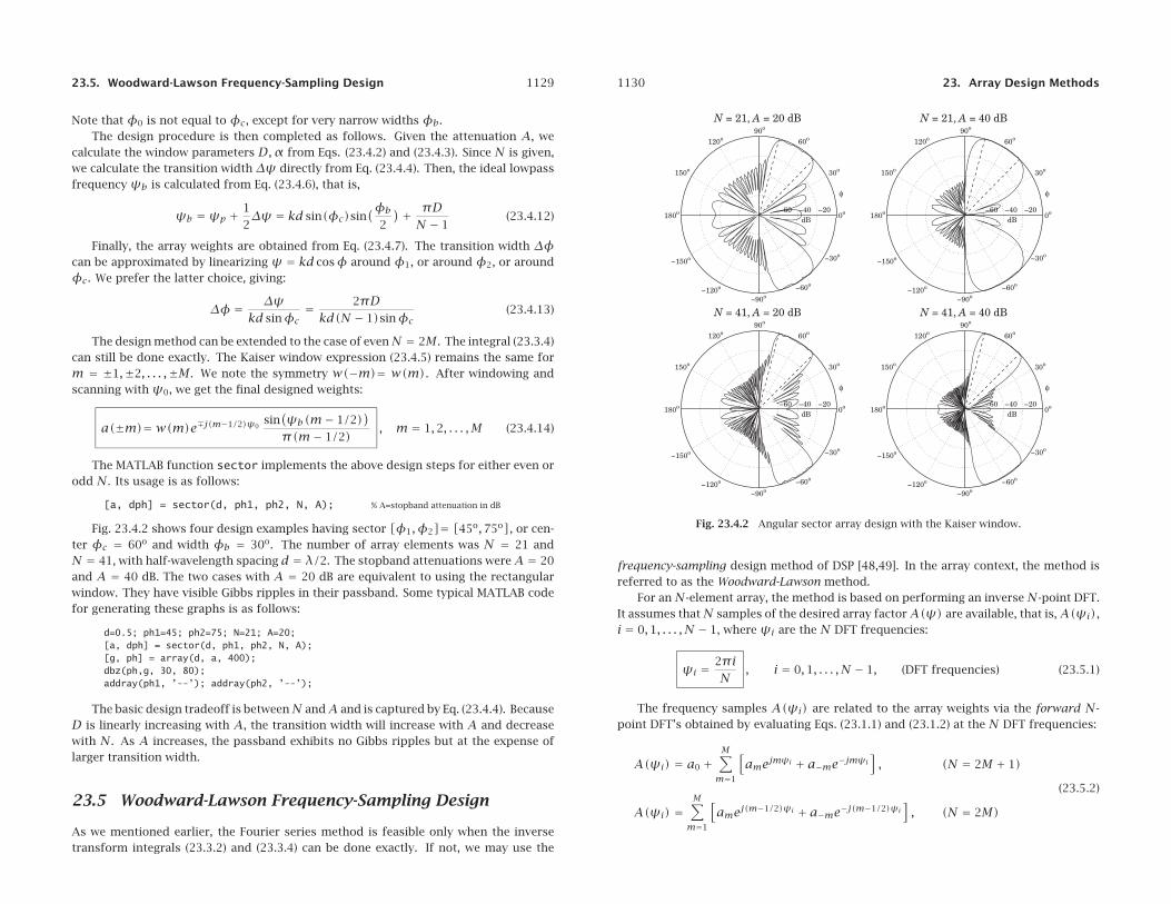
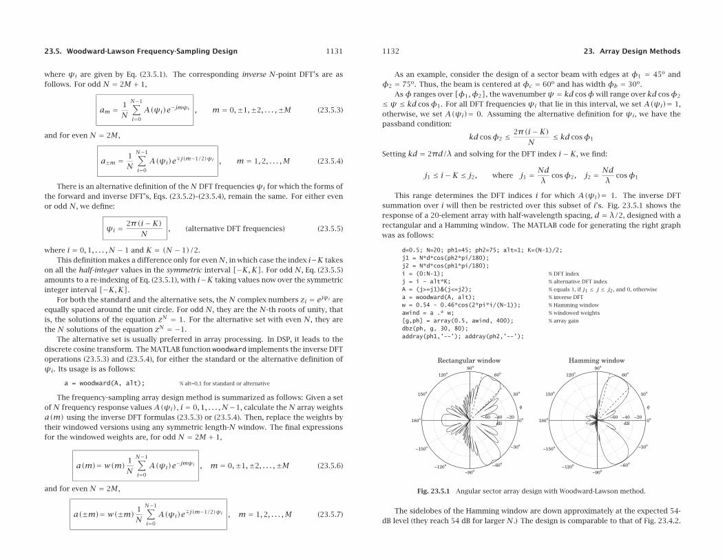
As an example, consider the design of a sector beam with edges at φ1 = 45o andφ2 = 75o. Thus, the beam is centered at φc = 60o and has width φb = 30o.

Asφ ranges over [φ1,φ2], the wavenumberψ = kd cosφ will range over kd cosφ2

≤ ψ ≤ kd cosφ1. For all DFT frequencies ψi that lie in this interval, we set A(ψi)= 1,otherwise, we set A(ψi)= 0. Assuming the alternative definition for ψi, we have thepassband condition:

kd cosφ2 ≤ 2π(i−K)N

≤ kd cosφ1

Setting kd = 2πd/λ and solving for the DFT index i−K, we find:

j1 ≤ i−K ≤ j2, where j1 = Ndλ cosφ2, j2 = Ndλ cosφ1

This range determines the DFT indices i for which A(ψi)= 1. The inverse DFTsummation over i will then be restricted over this subset of i’s. Fig. 23.5.1 shows theresponse of a 20-element array with half-wavelength spacing, d = λ/2, designed with arectangular and a Hamming window. The MATLAB code for generating the right graphwas as follows:

d=0.5; N=20; ph1=45; ph2=75; alt=1; K=(N-1)/2;j1 = N*d*cos(ph2*pi/180);j2 = N*d*cos(ph1*pi/180);i = (0:N-1); % DFT index

j = i - alt*K; % alternative DFT index

A = (j>=j1)&(j<=j2); % equals 1, if j1 ≤ j ≤ j2, and 0, otherwise

a = woodward(A, alt); % inverse DFT

w = 0.54 - 0.46*cos(2*pi*i/(N-1)); % Hamming window

awind = a .* w; % windowed weights

[g,ph] = array(0.5, awind, 400); % array gain

dbz(ph, g, 30, 80);addray(ph1,’--’); addray(ph2,’--’);

90o

−90o

0o180o

φ

60o

−60o

30o

−30o

120o

−120o

150o

−150o

−20−40−60dB

Rectangular window 90o

−90o

0o180o

φ

60o

−60o

30o

−30o

120o

−120o

150o

−150o

−20−40−60dB

Hamming window

Fig. 23.5.1 Angular sector array design with Woodward-Lawson method.

The sidelobes of the Hamming window are down approximately at the expected 54-dB level (they reach 54 dB for larger N.) The design is comparable to that of Fig. 23.4.2.


The power of this method lies in the ability to specify any shape for the array factorthrough its frequency samples. The method works well for half-wavelength spacingd = λ/2, because allN DFT frequenciesψi lie within the visible region, which coincidesin this case with the full Nyquist interval, −π ≤ ψ ≤ π.

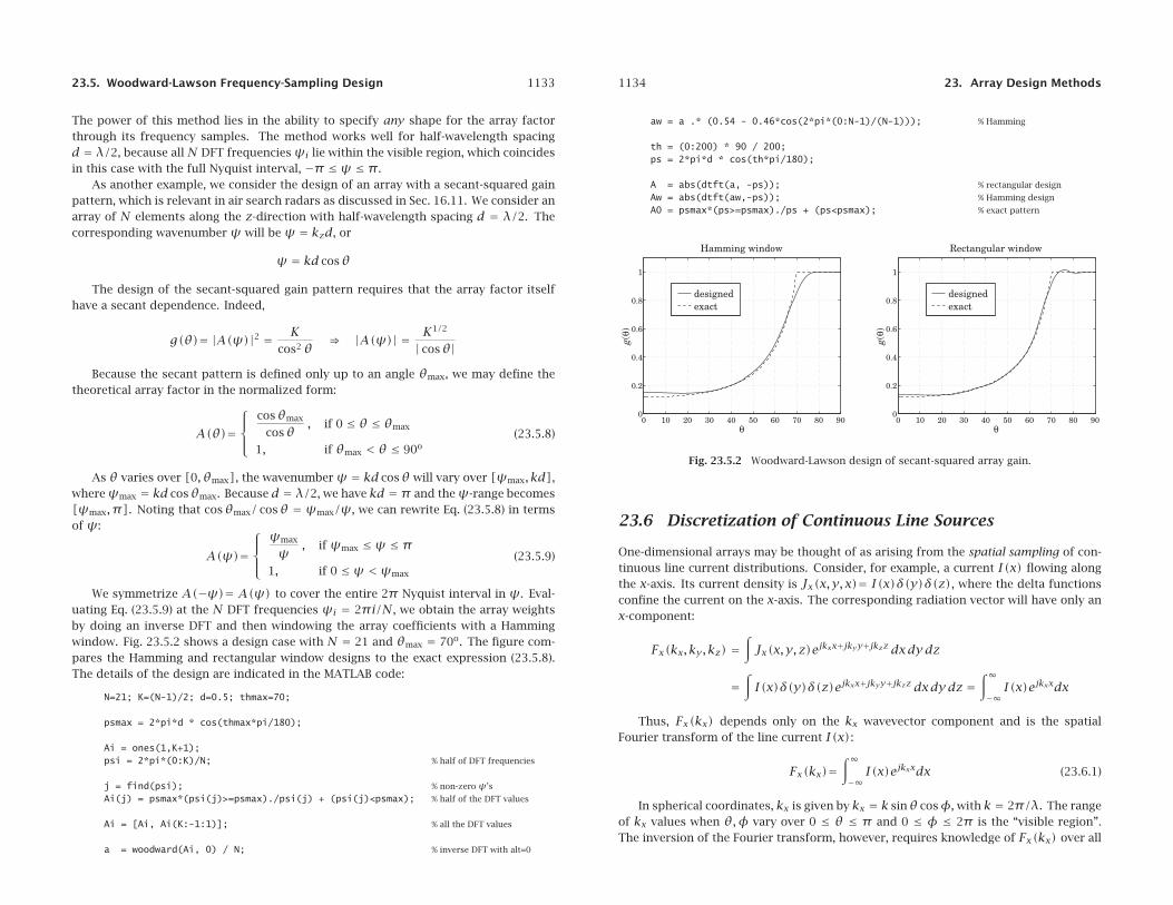
As another example, we consider the design of an array with a secant-squared gainpattern, which is relevant in air search radars as discussed in Sec. 16.11. We consider anarray of N elements along the z-direction with half-wavelength spacing d = λ/2. Thecorresponding wavenumber ψ will be ψ = kzd, or

ψ = kd cosθ

The design of the secant-squared gain pattern requires that the array factor itselfhave a secant dependence. Indeed,

g(θ)= |A(ψ)|2 = Kcos2 θ

⇒ |A(ψ)| = K1/2

| cosθ|Because the secant pattern is defined only up to an angle θmax, we may define the

theoretical array factor in the normalized form:

A(θ)=⎧⎪⎨⎪⎩

cosθmax

cosθ, if 0 ≤ θ ≤ θmax

1, if θmax < θ ≤ 90o(23.5.8)

As θ varies over [0, θmax], the wavenumberψ = kd cosθ will vary over [ψmax, kd],whereψmax = kd cosθmax. Because d = λ/2, we have kd = π and theψ-range becomes[ψmax,π]. Noting that cosθmax/ cosθ = ψmax/ψ, we can rewrite Eq. (23.5.8) in termsof ψ:

A(ψ)=⎧⎪⎨⎪⎩ψmax

ψ, if ψmax ≤ ψ ≤ π

1, if 0 ≤ ψ < ψmax

(23.5.9)

We symmetrize A(−ψ)= A(ψ) to cover the entire 2π Nyquist interval in ψ. Eval-uating Eq. (23.5.9) at the N DFT frequencies ψi = 2πi/N, we obtain the array weightsby doing an inverse DFT and then windowing the array coefficients with a Hammingwindow. Fig. 23.5.2 shows a design case with N = 21 and θmax = 70o. The figure com-pares the Hamming and rectangular window designs to the exact expression (23.5.8).The details of the design are indicated in the MATLAB code:

N=21; K=(N-1)/2; d=0.5; thmax=70;

psmax = 2*pi*d * cos(thmax*pi/180);

Ai = ones(1,K+1);psi = 2*pi*(0:K)/N; % half of DFT frequencies

j = find(psi); % non-zero ψ’s

Ai(j) = psmax*(psi(j)>=psmax)./psi(j) + (psi(j)<psmax); % half of the DFT values

Ai = [Ai, Ai(K:-1:1)]; % all the DFT values

a = woodward(Ai, 0) / N; % inverse DFT with alt=0


aw = a .* (0.54 - 0.46*cos(2*pi*(0:N-1)/(N-1))); % Hamming

th = (0:200) * 90 / 200;ps = 2*pi*d * cos(th*pi/180);

A = abs(dtft(a, -ps)); % rectangular design

Aw = abs(dtft(aw,-ps)); % Hamming design

A0 = psmax*(ps>=psmax)./ps + (ps<psmax); % exact pattern

0 10 20 30 40 50 60 70 80 900

0.2

0.4

0.6

0.8

1

Hamming window

θ

g(θ)

designedexact

0 10 20 30 40 50 60 70 80 900

0.2

0.4

0.6

0.8

1

Rectangular window

θ

g(θ)

designedexact

Fig. 23.5.2 Woodward-Lawson design of secant-squared array gain.

23.6 Discretization of Continuous Line Sources

One-dimensional arrays may be thought of as arising from the spatial sampling of con-tinuous line current distributions. Consider, for example, a current I(x) flowing alongthe x-axis. Its current density is Jx(x, y, x)= I(x)δ(y)δ(z), where the delta functionsconfine the current on the x-axis. The corresponding radiation vector will have only anx-component:

Fx(kx, ky, kz) =∫Jx(x, y, z)ejkxx+jkyy+jkzz dxdydz

=∫I(x)δ(y)δ(z)ejkxx+jkyy+jkzz dxdydz =

∫∞−∞I(x)ejkxxdx

Thus, Fx(kx) depends only on the kx wavevector component and is the spatialFourier transform of the line current I(x):

Fx(kx)=∫∞−∞I(x)ejkxxdx (23.6.1)

In spherical coordinates, kx is given by kx = k sinθ cosφ, with k = 2π/λ. The rangeof kx values when θ,φ vary over 0 ≤ θ ≤ π and 0 ≤ φ ≤ 2π is the “visible region”.The inversion of the Fourier transform, however, requires knowledge of Fx(kx) over all

23.6. Discretization of Continuous Line Sources 1135

kx, and in such case the inverse is:

I(x)= 1

2π

∫∞−∞Fx(kx)e−jkxx dkx (23.6.2)

Suppose now that the current I(x) is sampled at the regular intervals xm = mdwith spacing d and integer m. The sampled current may be represented as the sum ofimpulses:

I(x)=∞∑

m=−∞I(xm)δ(x− xm)=

∞∑m=−∞

Im δ(x−md) (23.6.3)

where we set Im = I(xm)= I(md). Then, the corresponding Fourier transform will be:

Fx(kx)=∫∞−∞I(x)ejkxxdx =

∞∑m=−∞

Im ejmkxd =∞∑

m=−∞Im ejmψ (23.6.4)

This has precisely the form of an array factor with ψ = kxd. The pattern Fx(kx)is periodic in kx with period ks = 2π/d, which is the sampling frequency in unitsof radians/meter. Equivalently, Fx(kx) is periodic in ψ with period 2π. The Poissonsummation formula [48] relates Fx(kx) to the unsampled pattern Fx(kx) as a sum ofshifted replicas:

Fx(kx)= 1

d

∞∑n=−∞

Fx(kx − nks) (23.6.5)

Aliasing, that is, the overlapping of the spectral replicas, can be avoided only ifFx(kx) is bandlimited to within the Nyquist interval, |kx| ≤ ks/2. This would imply thatI(x) have infinite extent.

In practice, I(x) is assumed to be space-limited with a finite extent, say, over an in-terval−l/2 ≤ x ≤ l/2. In this case, Fx(kx) cannot be bandlimited and therefore, aliasingwill always occur. However, if the pattern F(kx) attenuates with large kx, aliasing maybe minimized by selecting a small enough d.

Eqs. (23.6.4) and (23.6.5) provide two equivalent ways to express the spectrum of thesampled current. Eq. (23.6.4) can be inverted to recover the current samples Im:

Im = 1

ks

∫ ks/2−ks/2

Fx(kx)e−jmkxd dkx = 1

2π

∫ π−πFx(ψ)e−jmψ dψ (23.6.6)

which is the inverse discrete-space Fourier transform that we introduced in (22.4.8).By using the z-domain variable z = ejψ, (23.6.4) can also be written as the spatial z-transform:

Fx(z)=∞∑

m=−∞Im zn (23.6.7)

Next, we focus on finite line sources I(x), −l/2 ≤ x ≤ l/2. Then, (23.6.1) reads:

Fx(kx)=∫ l/2−l/2

I(x)ejkxx dx (23.6.8)

It proves convenient to define a normalized wavenumber variable u by:

u = lkx2π

� kx = 2πul

� u = lλ

sinθ cosφ (23.6.9)


and define a scaled pattern F(u)= Fx(kx)/l. Then, we have the Fourier relationships:

F(u)= 1

l

∫ l/2−l/2

I(x)ej2πux/l dx � I(x)=∫∞−∞F(u)e−j2πux/l du (23.6.10)

If I(x)were periodic with period l, then 2π/lwould be its fundamental harmonic and2πu/l would be interpreted as the uth harmonic. Indeed, the continuous-line versionof the Woodward-Lawson method gives u just such an interpretation. Let us define theperiodic extension of the space-limited I(x) with period l to be the sum of its replicas:

I(x)=∞∑

n=−∞I(x− nl) (23.6.11)

Then, I(x), being periodic, could be expanded in a Fourier series with coefficients:

I(x)=∞∑

p=−∞cp e−j2πpx/l , cp = 1

l

∫ l/2−l/2

I(x)ej2πpx/l dx (23.6.12)

Because I(x)= I(x) over the period −l/2 ≤ x ≤ l/2, the above integral for the pthcoefficient implies from (23.6.10) that cp = F(u) with u = p. Thus, restricting x overits basic period, we have the representation:

I(x)=∞∑

p=−∞F(p)e−j2πpx/l , − l

2≤ x ≤ l

2(23.6.13)

The pattern F(u) may itself be expressed in terms of its samples F(p). We havefrom (23.6.13):

F(u)= 1

l

∫ l/2−l/2

I(x)ej2πux/l dx =∞∑

p=−∞F(p)

1

l

∫ l/2−l/2

ej2π(u−p)x/l dx , or,

F(u)=∞∑

p=−∞F(p)

sin(π(u− p))π(u− p) (23.6.14)

Eqs. (23.6.13) and (23.6.14) are the continuous-line version of the Woodward-Lawsonmethod, which is of course equivalent to the application of Shannon’s sampling theoremto the space-limited function I(x), and our derivation is nothing more than the proofof that theorem.

For discrete arrays, we must sample in space xm =md, not in frequency. By takingN samples over the length l, that is, d = l/N, and truncating the summation in (23.6.13)to p = 0,1, . . . ,N− 1, we obtain the practical version of the Woodward-Lawson methodthat we used in the previous section.

For an N-element finite array, the z-transform Fx(z) of Eq. (23.6.7) becomes a poly-nomial of degree N − 1 in z. Such an array can be designed directly in discrete-spacedomain, or it can be designed by mapping a given continuous line source pattern to thediscrete case. This can be accomplished approximately by mapping N − 1 zeros of the

23.6. Discretization of Continuous Line Sources 1137

continuous pattern toN−1 zeros of the array using the mapping z = ejψ = ejkxd. Sinced = l/N, the mapping from u-space toψ-space becomesψ = kxd = 2πud/l = 2πu/N:

ψ = kxd = 2πuN

(23.6.15)

Therefore, if un, n = 1,2, . . . ,N−1 are theN−1 zeros of the pattern F(u) on whichthe design is to be based, then, we may define the corresponding zeros of the array by:

ψn = 2πunN

⇒ zn = ejψn = ej2πun/N , n = 1,2, . . . ,N − 1 (23.6.16)

and construct the array pattern polynomial from these zeros:

A(z)=N−1∏n=1

(z− zn) (23.6.17)

The method is an approximation because F(u) generally has an infinity of zeros.However, good results are obtained if N is large (e.g., N > 10).

To clarify the above definitions and Fourier relationships, we consider three exam-ples: (a) the uniform line source and how it relates to the uniform array, (b) Taylor’sone-parameter line source and its use to design Taylor-Kaiser arrays, and (c) Taylor’sideal line source, which is an idealization of the Chebyshev array, and leads to the so-called Taylor’s n distribution. A uniform line source has constant current:

I(x)=⎧⎨⎩1 , if − l/2 ≤ x ≤ l/2

0 , otherwise(23.6.18)

Its pattern is:

F(u)= 1

l

∫ l/2−l/2

I(x)ej2πux/l dx = 1

l

∫ l/2−l/2

ej2πux/l dx = sin(πu)πu

(23.6.19)

Its zeros are at the non-zero integers un = ±n, for n = 1,2, . . . . By selecting the firstN− 1 of these, un = n, for n = 1,2, . . . ,N− 1, we may map them to the N− 1 zeros ofthe uniform array:

zn = ej2πun/N = ej2πn/N , n = 1,2, . . . ,N − 1

The constructed array polynomial will be then,

A(z)= 1

N

N−1∏n=1

(z− zn)= 1

N

N−1∏n=1

(z− ej2πn/N) = 1

N

N−1∏n=0

(z− ej2πn/N)z− 1

where we introduced a scale factor 1/N and multiplied and divided by the factor (z−1).But the numerator polynomial, being a monic polynomial and having as roots the Nthroots of unity, must be equal to zN − 1. Thus,

A(z)= 1

NzN − 1

z− 1= 1

N(1+ z+ z2 + · · · + zN−1)


which has uniform array weights, am = 1/N. Replacing z = ejψ = ej2πu/N, we have:

A(ψ)= 1

NejψN − 1

ejψ − 1= sin(Nψ/2)N sin(ψ/2)

ejψ(N−1)/2 = sin(πu)N sin(πu/N)

ejπu(N−1)/N

For large N and fixed value of u, we may use the approximation sinx � x in thedenominator which tends to N sin(πu/N)� N(πu/N)= πu, thus, approximating thesinπu/πu pattern of the continuous line case.

Taylor’s one-parameter continuous line source [1262] has current I(x) and corre-sponding pattern F(u) given by the Fourier transform pair [194]:

F(u)=sinh

(π√B2 − u2

)π√B2 − u2

� I(x)= I0(πB√

1− (2x/l)2

)(23.6.20)

where −l/2 ≤ x ≤ l/2 and I0(·) is the modified Bessel function of first kind and zerothorder, and B is a positive parameter that controls the sidelobe level. For u > B, thepattern becomes a sinc-pattern in the variable

√u2 − B2, and for large u, it tends to the

pattern of the uniform line source. We will discuss this further in Sec. 23.10.Taylor’s ideal line source [1602] also has a parameter that controls the sidelobe level

and is is defined by the Fourier pair [194]:

F(u) = cosh(π√A2 − u2

)

I(x) =I1(πA

√1− (2x/l)2

)√

1− (2x/l)2

πAl+ δ

(x− l

2

)+ δ

(x+ l

2

) (23.6.21)

where I1(·) is the modified Bessel function of first kind and first order. Van der Maas[1250] showed first that this pair is the limit of a Dolph-Chebyshev array in the limit ofa large number of array elements. We will explore it further in Sec. 23.12.

23.7 Narrow-Beam Low-Sidelobe Designs

The problem of designing arrays having narrow beams with low sidelobes is equivalent tothe DSP problem of spectral analysis of windowed sinusoids. A single beam correspondsto a single sinusoid, multiple beams to multiple sinusoids.

To understand this equivalence, suppose one wants to design an infinitely narrowbeam toward some look direction φ = φ0. In ψ-space, the array factor (spatial orwavenumber spectrum) should be the infinitely thin spectral line:†

A(ψ)= 2πδ(ψ−ψ0)

where ψ = kd cosφ and ψ0 = kd cosφ0. Inserting this into the inverse DSFT ofEq. (23.3.2), gives the double-sided infinitely-long array, for −∞ < m <∞:

a(m)= 1

2π

∫ π−πA(ψ)e−jmψdψ = 1

2π

∫ π−π

2πδ(ψ−ψ0)e−jmψdψ = e−jψ0m

†To be periodic in ψ, all the Nyquist replicas of this term must be added. But they are not shown herebecause ψ0 and ψ are assumed to lie in the central Nyquist interval [−π,π].

23.7. Narrow-Beam Low-Sidelobe Designs 1139

This is the spatial analog of an infinite sinusoid a(n)= ejω0n whose spectrum is thesharp spectral line A(ω)= 2πδ(ω −ω0). A finite-duration sinusoid is obtained bywindowing with a length-N time window w(n) resulting in a(n)= w(n)ejω0n.

In the frequency domain, the effect of windowing is to replace the spectral lineδ(ω−ω0) by its smeared versionW(ω−ω0), whereW(ω) is the DTFT of the windoww(n). The spectrum W(ω −ω0) exhibits a main lobe at ω = ω0 and sidelobes. Themain lobe gets narrower with increasing N.

A finiteN-element array with a narrow beam and low sidelobes, and steered towardsan angle φ0, can be obtained by windowing the infinite narrow-beam array with anappropriate length-N spatial window w(m). For odd N = 2M+ 1, or even N = 2M, wedefine respectively:

a(m) = e−jmψ0w(m), m = 0,±1,±2, . . . ,±Ma(±m) = e∓j(m−1/2)ψ0w(±m), m = 1,2, . . . ,M

(23.7.1)

In both cases, the array factor of Eqs. (23.1.1) and (23.1.2) becomes:

A(ψ)=W(ψ−ψ0) (narrow beam array factor) (23.7.2)

whereW(ψ) is the DSFT of the window, defined for odd or even N as:

W(ψ) = w(0)+M∑m=1

[w(m)ejmψ +w(−m)e−jmψ

]

W(ψ) =M∑m=1

[w(m)ej(m−1/2)ψ +w(−m)e−j(m−1/2)ψ

] (23.7.3)

Assuming a symmetric window, w(−m)= w(m), we can rewrite:

W(ψ) = w(0)+2M∑m=1

w(m)cos(mψ)

W(ψ) = 2M∑m=1

w(m)cos((m− 1/2)ψ

)(N = 2M + 1)

(N = 2M)

(23.7.4)

At broadside,ψ0 = 0,φ0 = 90o, Eq. (23.7.1) reduces to a(m)= w(m) and the arrayfactor becomesA(ψ)=W(ψ). Thus, the weights of a broadside narrow beam array arethe window samples a(m)= w(m). The steered weights (23.7.1) can be calculated withthe help of the MATLAB function scan, or steer:

a = scan(w, psi0);

a = steer(d, w, phi0);

The primary issue in choosing a window function w(m) is the tradeoff between fre-quency resolution and frequency leakage, that is, between main-lobe width and sidelobe


level [48,49]. Ideally, one would like to meet, as best as possible, the two conflictingrequirements of having a very narrow mainlobe and very small sidelobes.

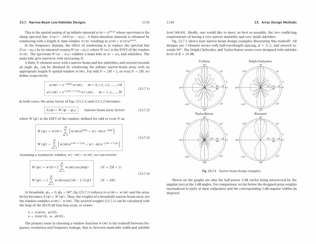
Fig. 23.7.1 shows four narrow-beam design examples illustrating this tradeoff. Alldesigns are 7-element arrays with half-wavelength spacing, d = λ/2, and steered to-wards 90o. The Dolph-Chebyshev and Taylor-Kaiser arrays were designed with sidelobelevel of R = 20 dB.

90o

−90o

0o180o

φ

45o

−45o

135o

−135o

−10−20−30dB

Uniform 90o

−90o

0o180o

φ

45o

−45o

135o

−135o

−10−20−30dB

Dolph−Chebyshev

90o

−90o

0o180o

φ

45o

−45o

135o

−135o

−10−20−30dB

Taylor−Kaiser 90o

−90o

0o180o

φ

45o

−45o

135o

−135o

−10−20−30dB

Binomial

Fig. 23.7.1 Narrow beam design examples.

Shown on the graphs are also the half-power 3-dB circles being intersected by theangular rays at the 3-dB angles. For comparison, we list below the designed array weights(normalized to unity at their endpoints) and the corresponding 3-dB angular widths (indegrees):

23.7. Narrow-Beam Low-Sidelobe Designs 1141

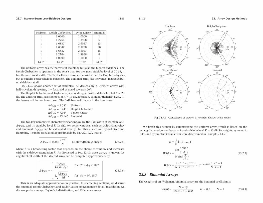
Uniform Dolph-Chebyshev Taylor-Kaiser Binomial1 1.0000 1.0000 11 1.2764 1.8998 61 1.6837 2.6057 151 1.8387 2.8728 201 1.6837 2.6057 151 1.2764 1.8998 61 1.0000 1.0000 1

14.5o 16.4o 16.8o 24.6o

The uniform array has the narrowest mainlobe but also the highest sidelobes. TheDolph-Chebyshev is optimum in the sense that, for the given sidelobe level of 20 dB, ithas the narrowest width. The Taylor-Kaiser is somewhat wider than the Dolph-Chebyshev,but it exhibits better sidelobe behavior. The binomial array has the widest mainlobe butno sidelobes at all.

Fig. 23.7.2 shows another set of examples. All designs are 21-element arrays withhalf-wavelength spacing, d = λ/2, and scanned towards 60o.

The Dolph-Chebyshev and Taylor arrays were designed with sidelobe level of R = 25dB. The uniform array has sidelobes atR = 13 dB. BecauseN is higher than in Fig. 23.7.1,the beams will be much narrower. The 3-dB beamwidths are in the four cases:

Δφ3dB = 5.58o UniformΔφ3dB = 6.44o Dolph-ChebyshevΔφ3dB = 7.03o Taylor-KaiserΔφ3dB = 15.64o Binomial

The two key parameters characterizing a window are the 3-dB width of its main lobe,Δψ3dB, and its sidelobe level R (in dB). For some windows, such as Dolph-Chebyshevand binomial, Δψ3dB can be calculated exactly. In others, such as Taylor-Kaiser andHamming, it can be calculated approximately by Eq. (22.10.2), that is,

Δψ3dB = 0.8862πbN

(3-dB width in ψ-space) (23.7.5)

where b is a broadening factor that depends on the choice of window and increaseswith the sidelobe attenuation R. As discussed in Sec. 22.10, once Δψ3dB is known, theangular 3-dB width of the steered array can be computed approximately by:

Δφ3dB =

⎧⎪⎪⎪⎪⎪⎨⎪⎪⎪⎪⎪⎩

Δψ3dB

kd sinφ0, for 0o < φ0 < 180o

2

√Δψ3dB

kd, for φ0 = 0o, 180o

(23.7.6)

This is an adequate approximation in practice. In succeeding sections, we discussthe binomial, Dolph-Chebyshev, and Taylor-Kaiser arrays in more detail. In addition, wediscuss prolate arrays, Taylor’s n distribution, and Villeneuve arrays.


90o

−90o

0o180o

φ

60o

−60o

30o

−30o

120o

−120o

150o

−150o

−10−20−30dB

Uniform 90o

−90o

0o180o

φ

60o

−60o

30o

−30o

120o

−120o

150o

−150o

−10−20−30dB

Dolph−Chebyshev

90o

−90o

0o180o

φ

60o

−60o

30o

−30o

120o

−120o

150o

−150o

−10−20−30dB

Taylor−Kaiser 90o

−90o

0o180o

φ

60o

−60o

30o

−30o

120o

−120o

150o

−150o

−10−20−30dB

Binomial

Fig. 23.7.2 Comparison of steered 21-element narrow-beam arrays.

We finish this section by summarizing the uniform array, which is based on therectangular window and has b = 1 and sidelobe level R = 13 dB. Its weights, symmetricDSFT, and symmetric z-transform were determined in Example 23.1.2:

w = 1

N[1,1, . . . ,1]

W(ψ) =sin(Nψ

2

)

N sin(ψ2

)

W(z) = 1

NzN/2 − z−N/2z1/2 − z−1/2 = z−(N−1)/2 1

NzN − 1

z− 1

(23.7.7)

23.8 Binomial Arrays

The weights of an N-element binomial array are the binomial coefficients:

w(m)= (N − 1)!m!(N − 1−m)! , m = 0,1, . . . ,N − 1 (23.8.1)

23.8. Binomial Arrays 1143

For example, for N = 4 and N = 5 they are:

w = [1,3,3,1]w = [1,4,6,4,1]

The binomial weights are the expansion coefficients of the polynomial (1 + z)N−1. In-deed, the symmetric z-transform of the binomial array is defined as:

W(z)= (z1/2 + z−1/2)N−1 = z−(N−1)/2(1+ z)N−1 (23.8.2)

Setting z = ejψ, we find the array factor in ψ-space:

W(ψ)= (ejψ/2 + e−jψ/2)N−1 =[

2 cos(ψ

2

)]N−1

(23.8.3)

This response falls monotonically on either side of the peak atψ = 0 until it becomeszero at the Nyquist frequency ψ = ±π. Indeed, the z-transform has a multiple zero oforder N − 1 at z = −1.

Thus, the binomial response has no sidelobes. This is, of course, at the expense ofa fairly wide mainlobe. The 3-dB width Δψ3dB can be determined by finding the 3-dBfrequencies ±ψ3 that satisfy the half-power condition:

|W(ψ3)|2|W(0)|2 = 1

2⇒

[cos(ψ3

2

)]2(N−1)= 1

2

The solution is:ψ3 = 2 acos

(2−0.5/(N−1))

Therefore, the 3-dB width will be Δψ3dB = 2ψ3:

Δψ3dB = 4 acos(

2−0.5/(N−1))

(23.8.4)

Once Δψ3dB is found, the 3-dB width Δφ3dB in angle space, for an array steeredtowards an angle φ0, can be found from Eq. (23.7.6). The MATLAB function binomialgenerates the array weights (steered towards φ0) and 3-dB width. Its usage is:

[a, dph] = binomial(d, ph0, N); % binomial array coefficients and beamwidth

For example, the fourth graph of the binomial response of Fig. 23.7.1 was generatedby the MATLAB code:

[a, dph] = binomial(0.5, 90, 5); % array weights and 3-dB width

[g, ph] = array(0.5, a, 200); % compute array gain

dbz(ph, g, 45, 40); % plot gain in dB with 40-dB scale

addcirc(3, 40, ’--’); % add 3-dB grid circle

addray(90 + dph/2, ’-’); % add rays at 3-dB angles

addray(90 - dph/2, ’-’);


23.9 Dolph-Chebyshev Arrays

Most windows have largest sidelobes near the main lobe. If a window is designed toachieve a minimum sidelobe attenuation of R dB, then typically R will be the atten-uation of the sidelobes nearest to the mainlobe; the sidelobes further away will haveattenuations higher than R.

Because of the tradeoff between mainlobe width and sidelobe attenuation, the extraattenuation of the furthest sidelobes will come at the expense of increased mainlobewidth. If the attenuation of these sidelobes could be decreased (up to the level of theminimum R), then the mainlobe width would narrow.

It follows that for a given minimum desired sidelobe levelR, the narrowest mainlobewidth will be achieved by a window whose sidelobes are all equal to R. Conversely,for a given maximum desired mainlobe width, the largest sidelobe attenuation will beachieved by a window with equal sidelobe levels.

This “optimum” window is the Dolph-Chebyshev window, which is constructed withthe help of Chebyshev polynomials. Themth Chebyshev polynomial Tm(x) is:

Tm(x)= cos(m acos(x)

)(23.9.1)

If |x| > 1, the inverse cosine acos(x) becomes imaginary, and the expression can berewritten in terms of hyperbolic cosines: Tm(x)= cosh

(m acosh(x)

).

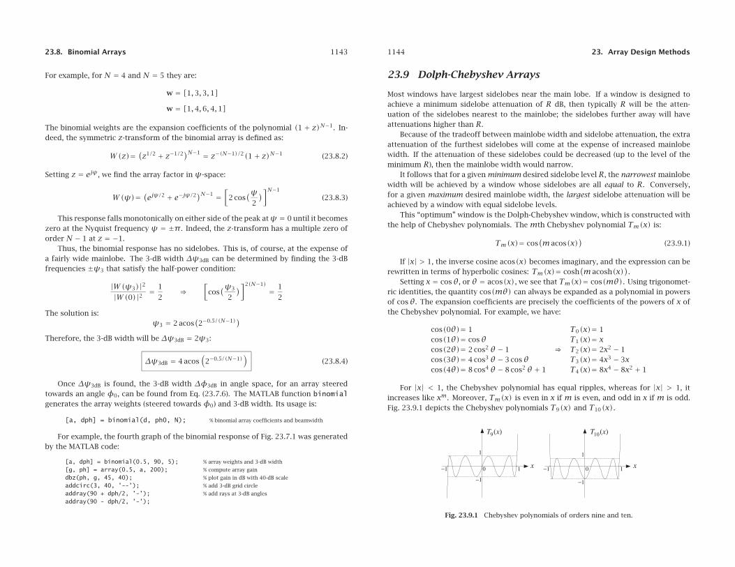
Setting x = cosθ, or θ = acos(x), we see that Tm(x)= cos(mθ). Using trigonomet-ric identities, the quantity cos(mθ) can always be expanded as a polynomial in powersof cosθ. The expansion coefficients are precisely the coefficients of the powers of x ofthe Chebyshev polynomial. For example, we have:

cos(0θ)= 1 T0(x)= 1cos(1θ)= cosθ T1(x)= xcos(2θ)= 2 cos2 θ− 1 ⇒ T2(x)= 2x2 − 1cos(3θ)= 4 cos3 θ− 3 cosθ T3(x)= 4x3 − 3xcos(4θ)= 8 cos4 θ− 8 cos2 θ+ 1 T4(x)= 8x4 − 8x2 + 1

For |x| < 1, the Chebyshev polynomial has equal ripples, whereas for |x| > 1, itincreases like xm. Moreover, Tm(x) is even in x if m is even, and odd in x if m is odd.Fig. 23.9.1 depicts the Chebyshev polynomials T9(x) and T10(x).

Fig. 23.9.1 Chebyshev polynomials of orders nine and ten.

23.9. Dolph-Chebyshev Arrays 1145

The Dolph-Chebyshev window is defined such that its sidelobes will correspond toa portion of the equi-ripple range |x| ≤ 1 of the Chebyshev polynomial, whereas itsmainlobe will correspond to a portion of the range x > 1.

For either even or odd N, Eq. (23.7.4) implies that any window spectrumW(ψ) canbe written in general as a polynomial of degree N − 1 in the variable u = cos(ψ/2).Indeed, we have for themth terms:

cos(mψ)= cos(

2mψ2

)= T2m(u)

cos((m− 1/2)ψ)= cos

((2m− 1)

ψ2

)= T2m−1(u)

Thus in the odd case, the summation in Eq. (23.7.4) will result in a polynomial ofmaximal degree 2M = N − 1 in the variable u, and in the even case, it will result into apolynomial of degree 2M − 1 = N − 1.

The Dolph-Chebyshev [1244] array factor is defined by the Chebyshev polynomial ofdegree N − 1 in the scaled variable x = x0 cos(ψ/2), that is,

W(ψ)= TN−1(x), x = x0 cos(ψ2

)(Dolph-Chebyshev array factor) (23.9.2)

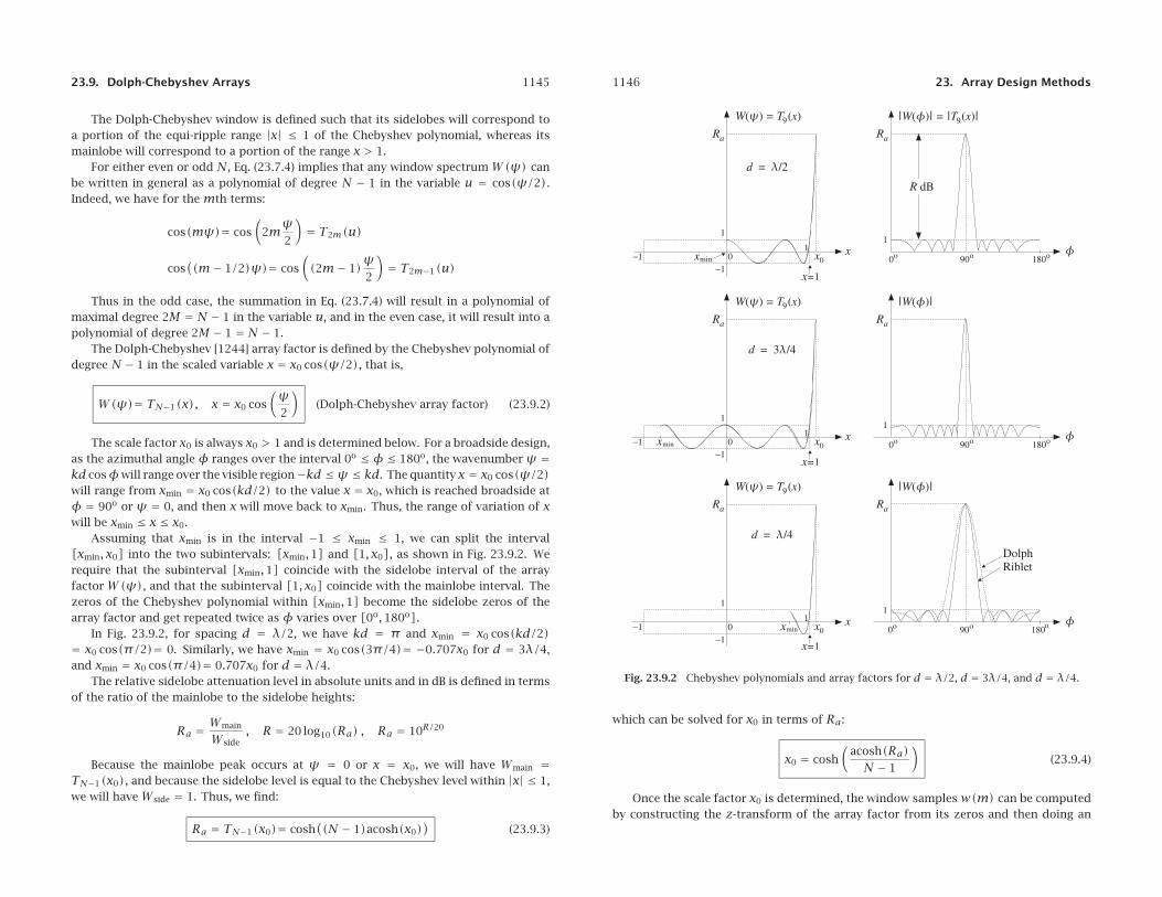
The scale factor x0 is always x0 > 1 and is determined below. For a broadside design,as the azimuthal angle φ ranges over the interval 0o ≤ φ ≤ 180o, the wavenumberψ =kd cosφwill range over the visible region−kd ≤ ψ ≤ kd. The quantity x = x0 cos(ψ/2)will range from xmin = x0 cos(kd/2) to the value x = x0, which is reached broadside atφ = 90o or ψ = 0, and then x will move back to xmin. Thus, the range of variation of xwill be xmin ≤ x ≤ x0.

Assuming that xmin is in the interval −1 ≤ xmin ≤ 1, we can split the interval[xmin, x0] into the two subintervals: [xmin,1] and [1, x0], as shown in Fig. 23.9.2. Werequire that the subinterval [xmin,1] coincide with the sidelobe interval of the arrayfactor W(ψ), and that the subinterval [1, x0] coincide with the mainlobe interval. Thezeros of the Chebyshev polynomial within [xmin,1] become the sidelobe zeros of thearray factor and get repeated twice as φ varies over [0o,180o].

In Fig. 23.9.2, for spacing d = λ/2, we have kd = π and xmin = x0 cos(kd/2)= x0 cos(π/2)= 0. Similarly, we have xmin = x0 cos(3π/4)= −0.707x0 for d = 3λ/4,and xmin = x0 cos(π/4)= 0.707x0 for d = λ/4.

The relative sidelobe attenuation level in absolute units and in dB is defined in termsof the ratio of the mainlobe to the sidelobe heights:

Ra = Wmain

Wside, R = 20 log10(Ra) , Ra = 10R/20

Because the mainlobe peak occurs at ψ = 0 or x = x0, we will have Wmain =TN−1(x0), and because the sidelobe level is equal to the Chebyshev level within |x| ≤ 1,we will haveWside = 1. Thus, we find:

Ra = TN−1(x0)= cosh((N − 1)acosh(x0)

)(23.9.3)


Fig. 23.9.2 Chebyshev polynomials and array factors for d = λ/2, d = 3λ/4, and d = λ/4.

which can be solved for x0 in terms of Ra:

x0 = cosh(

acosh(Ra)N − 1

)(23.9.4)

Once the scale factor x0 is determined, the window samplesw(m) can be computedby constructing the z-transform of the array factor from its zeros and then doing an


inverse z-transform. The N − 1 zeros of TN−1(x) are easily found to be:

TN−1(x)= cos((N − 1)acos(x)

) = 0 ⇒ xi = cos((i− 1/2)πN − 1

)

for i = 1,2, . . . ,N − 1. Solving for the corresponding wavenumbers through xi =x0 cos(ψi/2), we find the pattern zeros:

ψi = 2 acos( xix0

), zi = ejψi , i = 1,2, . . . ,N − 1

We note that the zeros xi do not have to lie within the sidelobe range [xmin,1] andthe corresponding ψi do not all have to be in the visible region.

The symmetric z-transform of the window is constructed in terms of the one-sidedtransform using Eq. (23.1.4) as follows:

W(z)= z−(N−1)/2 W(z)= z−(N−1)/2N−1∏i=1

(z− zi) (23.9.5)

The inverse z-transform of W(z) are the window coefficients w(m). The MATLABfunction dolph.m of Appendix L implements this design procedure with the help ofthe function poly2.m, which calculates the coefficients from the zeros.† The typicalMATLAB code in dolph.m is as follows:

N1 = N-1; % number of zeros

Ra = 10^(R/20); % sidelobe level in absolute units

x0 = cosh(acosh(Ra)/N1); % scaling factor

i = 1:N1;xi = cos(pi*(i-0.5)/N1); % N1 zeros of Chebyshev polynomial

psi = 2 * acos(xi/x0); % N1 array pattern zeros in psi-space

zi = exp(j*psi); % N1 zeros of array polynomial

a = real(poly2(zi)); % zeros-to-polynomial form (N coefficients)

The window coefficients resulting from definition (23.9.5) are normalized to unityvalues at their end-points. This definition differs from that of Eq. (23.9.2) by the scalefactor xN−1

0 /2.The function dolph.m also returns the 3-dB width of the main lobe. The 3-dB fre-

quency ψ3 is defined by the half-power condition:

W(ψ3)= TN−1(x3)= TN−1(x0)√2

= Ra√2

⇒ cosh((N − 1)acosh(x3)

) = Ra√2

Solving for x3 and the corresponding 3-dB angle, x3 = x0 cos(ψ3/2), we have:

x3 = cosh

(acosh(Ra/

√2)

N − 1

), ψ3 = 2 acos

(x3

x0

)(23.9.6)

which yields the 3-dB width in ψ-space, Δψ3dB = 2ψ3. The 3-dB width in angle space,Δφ3dB, is then computed from Eq. (23.7.6) or (22.10.6).

†See Sec. 6.8 regarding the accuracy of poly2 versus poly.


There exist several alternative methods for calculating the Chebyshev array coeffi-cients [1248–1257,1259] and have been compared in [1258]. One particularly accurateand effective method is that of Bresler [1252], which has recently been implemented bySimon [1254] with the MATLAB function chebarray.m.

Example 23.9.1: The second graph of Fig. 23.7.1 was generated by the MATLAB commands:

[a, dph] = dolph(0.5, 90, 5, 20); % array weights and 3-dB width

[g, ph] = array(0.5, a, 200); % compute array gain

dbz(ph, g, 45); % plot gain in dB

addcirc(3, 40, ’--’); % add 3-dB gain circle

addray(90 + dph/2, ’--’); % add 3-dB angles

addray(90 - dph/2, ’--’);

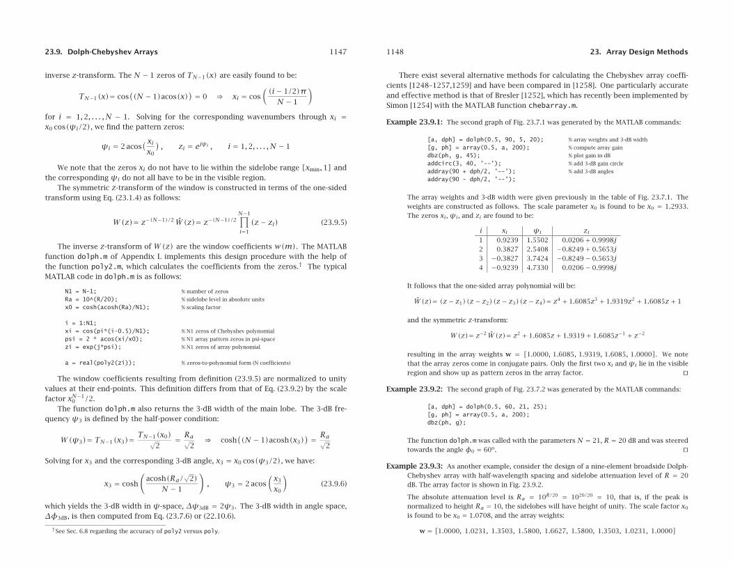
The array weights and 3-dB width were given previously in the table of Fig. 23.7.1. Theweights are constructed as follows. The scale parameter x0 is found to be x0 = 1.2933.The zeros xi, ψi, and zi are found to be:

i xi ψi zi1 0.9239 1.5502 0.0206+ 0.9998j2 0.3827 2.5408 −0.8249+ 0.5653j3 −0.3827 3.7424 −0.8249− 0.5653j4 −0.9239 4.7330 0.0206− 0.9998j

It follows that the one-sided array polynomial will be:

W(z)= (z− z1)(z− z2)(z− z3)(z− z4)= z4 + 1.6085z3 + 1.9319z2 + 1.6085z+ 1

and the symmetric z-transform:

W(z)= z−2 W(z)= z2 + 1.6085z+ 1.9319+ 1.6085z−1 + z−2

resulting in the array weights w = [1.0000, 1.6085, 1.9319, 1.6085, 1.0000]. We notethat the array zeros come in conjugate pairs. Only the first two xi and ψi lie in the visibleregion and show up as pattern zeros in the array factor. ��

Example 23.9.2: The second graph of Fig. 23.7.2 was generated by the MATLAB commands:

[a, dph] = dolph(0.5, 60, 21, 25);[g, ph] = array(0.5, a, 200);dbz(ph, g);

The function dolph.m was called with the parameters N = 21, R = 20 dB and was steeredtowards the angle φ0 = 60o. ��

Example 23.9.3: As another example, consider the design of a nine-element broadside Dolph-Chebyshev array with half-wavelength spacing and sidelobe attenuation level of R = 20dB. The array factor is shown in Fig. 23.9.2.

The absolute attenuation level is Ra = 10R/20 = 1020/20 = 10, that is, if the peak isnormalized to height Ra = 10, the sidelobes will have height of unity. The scale factor x0

is found to be x0 = 1.0708, and the array weights:

w = [1.0000, 1.0231, 1.3503, 1.5800, 1.6627, 1.5800, 1.3503, 1.0231, 1.0000]


The array zeros are constructed as follows:

i xi ψi zi1 0.9808 0.8260 0.6778+ 0.7352j2 0.8315 1.3635 0.2059+ 0.9786j3 0.5556 2.0506 −0.4616+ 0.8871j4 0.1951 2.7752 −0.9336+ 0.3583j5 −0.1951 3.5080 −0.9336− 0.3583j6 −0.5556 4.2326 −0.4616− 0.8871j7 −0.8315 4.9197 0.2059− 0.9786j8 −0.9808 5.4572 0.6778− 0.7352j

The 3-dB width is found from Eq. (23.9.6) to be Δφ3dB = 12.51o. ��

In order for the Chebyshev interval [xmin,1] to be mapped onto the sidelobe regionof the array factor, we must require that xmin ≥ −1.

If d < λ/2, then this condition is automatically satisfied because kd < π/2 andxmin = x0 cos(kd/2)> 0. (In this case, we must also demand that xmin ≤ 1. However,as we discuss below, when d < λ/2 Dolph’s construction is no longer optimal and isreplaced by the alternative procedure of Riblet.)

If λ/2 < d < λ, then π < kd < 2π and xmin < 0 and can exceed the left limitx = −1. This requires that for the given sidelobe level R, the array spacing may notexceed a maximum value that satisfies xmin = x0 cos(kdmax/2)= −1. This gives:

kdmax = 2 acos(− 1

x0

)⇒ dmax = λπ acos

(− 1

x0

)(23.9.7)

An alternative way of phrasing the condition xmin ≥ −1 is to say that for the givenvalue of the array spacing d (such that λ/2 < d < λ), there is a maximum sidelobeattenuation that may be designed. The corresponding maximum value of x0 will satisfyxmin = x0,max cos(kd/2)= −1, which gives:

x0,max = − 1

cos(kd/2)⇒ Ra,max = TN−1(x0,max) (23.9.8)

Example 23.9.4: Consider the case d = 3λ/4, R = 20 dB, N = 9. Then for the given R, themaximum element spacing that we can have is dmax = 0.8836λ.

Alternatively, for the given spacing d = 3λ/4, the maximum sidelobe attenuation that wecan have is Ra,max = 577, or, Rmax = 55.22 dB.

An array designed with the maximum spacing d = dmax will have the narrowest mainlobe,because its total length will be the longest possible. For example, the following two callsto the function dolph will calculate the required 3-dB beamwidths:

[w, dph1] = dolph(0.75, 90, 9, 20); % spacing d = 3/4

[w, dph2] = dolph(0.8836, 90, 9, 20); % spacing d = dmax

We find Δφ1 = 8.34o and Δφ2 = 7.08o. The array weights w are the same in the two casesand equal to those of Example 23.9.3. The gains are shown in Fig. 23.9.3. ��


90o

−90o

0o180o

φ

60o

−60o

30o

−30o

120o

−120o

150o

−150o

−10−20−30dB

d = 0.75λ 90o

−90o

0o180o

φ

60o

−60o

30o

−30o

120o

−120o

150o

−150o

−10−20−30dB

d = dmax = 0.8836λ

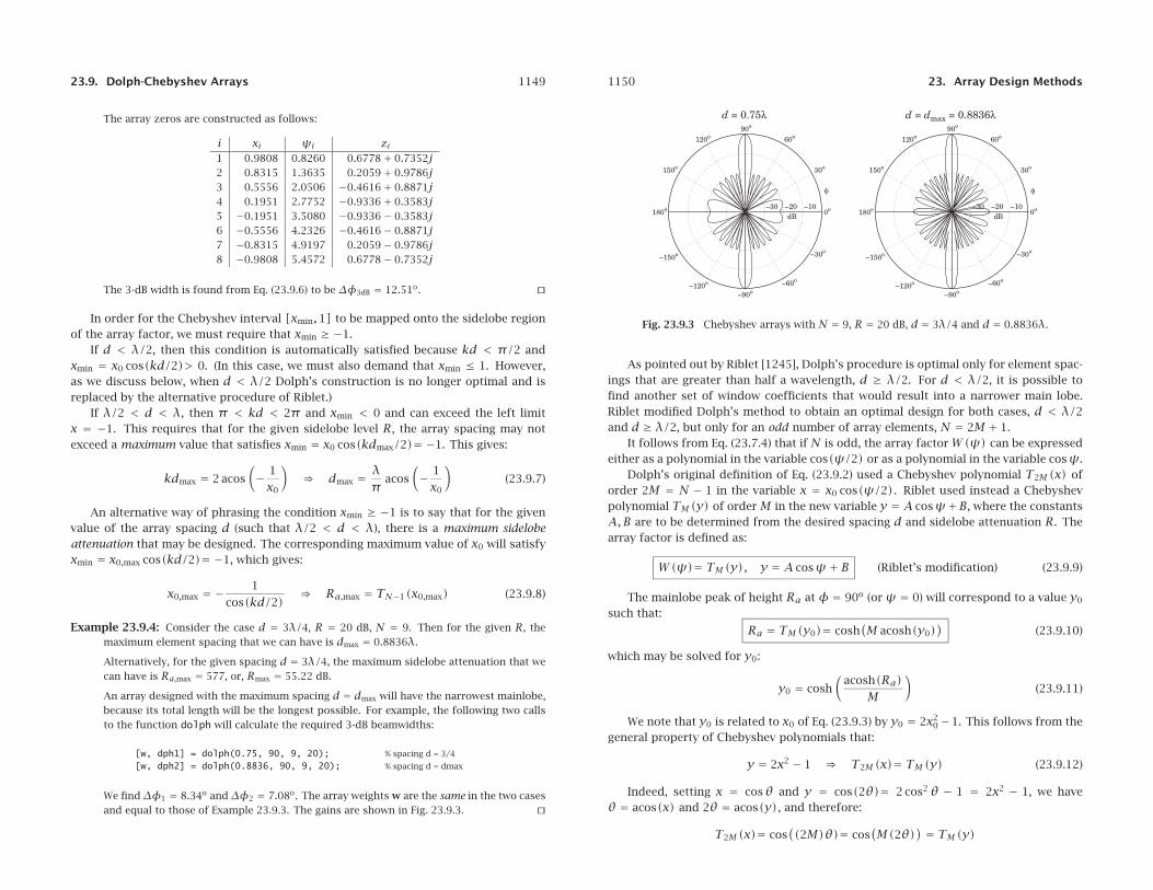
Fig. 23.9.3 Chebyshev arrays with N = 9, R = 20 dB, d = 3λ/4 and d = 0.8836λ.

As pointed out by Riblet [1245], Dolph’s procedure is optimal only for element spac-ings that are greater than half a wavelength, d ≥ λ/2. For d < λ/2, it is possible tofind another set of window coefficients that would result into a narrower main lobe.Riblet modified Dolph’s method to obtain an optimal design for both cases, d < λ/2and d ≥ λ/2, but only for an odd number of array elements, N = 2M + 1.

It follows from Eq. (23.7.4) that if N is odd, the array factorW(ψ) can be expressedeither as a polynomial in the variable cos(ψ/2) or as a polynomial in the variable cosψ.

Dolph’s original definition of Eq. (23.9.2) used a Chebyshev polynomial T2M(x) oforder 2M = N − 1 in the variable x = x0 cos(ψ/2). Riblet used instead a Chebyshevpolynomial TM(y) of orderM in the new variable y = A cosψ+B, where the constantsA,B are to be determined from the desired spacing d and sidelobe attenuation R. Thearray factor is defined as:

W(ψ)= TM(y), y = A cosψ+ B (Riblet’s modification) (23.9.9)

The mainlobe peak of height Ra at φ = 90o (orψ = 0) will correspond to a value y0

such that:

Ra = TM(y0)= cosh(M acosh(y0)

)(23.9.10)

which may be solved for y0:

y0 = cosh(

acosh(Ra)M

)(23.9.11)

We note that y0 is related to x0 of Eq. (23.9.3) by y0 = 2x20−1. This follows from the

general property of Chebyshev polynomials that:

y = 2x2 − 1 ⇒ T2M(x)= TM(y) (23.9.12)

Indeed, setting x = cosθ and y = cos(2θ)= 2 cos2 θ − 1 = 2x2 − 1, we haveθ = acos(x) and 2θ = acos(y), and therefore:

T2M(x)= cos((2M)θ)= cos

(M(2θ)

) = TM(y)


As the azimuthal angle φ varies over 0o ≤ φ ≤ 180o and the wavenumber ψ overthe visible region −kd ≤ ψ ≤ kd, the quantity c = cosψ will vary from c = cos(kd) atφ = 0o to c = 1 at φ = 90o, and then back to c = cos(kd) at φ = 180o.

If λ/2 ≤ d ≤ λ, then π ≤ kd ≤ 2π and ψ = kd cosφ will pass through the valueψ = π before it reaches the valueψ = kd. It follows that the quantity c will go throughc = −1 before it reaches c = cos(kd). Thus, in this case the widest range of variationof c = cosψ is −1 ≤ c ≤ 1.

On the other hand, if d < λ/2, then kd < π and c never reaches the value c = −1.Its minimum value is c = cos(kd), and the range of c is [cos(kd),1]. To summarize,the range of variation of c will be the interval [c0,1], where

c0 ={−1, if d ≥ λ/2cos(kd), if d < λ/2 (23.9.13)

Assuming A > 0, it follows that the range of variation of y = A cosψ+B will be theinterval [Ac0 +B, A+B]. The parameters A,B are fixed by requiring that this intervalcoincide with the interval [−1, y0] so that the right end will correspond to the mainlobepeak, while the left end will ensure that we use the maximum size of the equi-rippleinterval of the Chebyshev variable y. Thus, we require the conditions:

Ac0 + B = −1

A+ B = y0

(23.9.14)

which may be solved for A,B:

A = 1+ y0

1− c0

B = −1+ y0c0

1− c0

(23.9.15)

For d ≥ λ/2, the method coincides with Dolph’s original method. In this case,c0 = −1, and A,B become:

A = y0 + 1

2= x2

0

B = y0 − 1

2= x2

0 − 1

(23.9.16)

where we used y0 = 2x20 − 1, as discussed above. It follows that the y variable will be

related to the Dolph variable x = x0 cos(ψ/2) by:

y = x20 cosψ+ x2

0 − 1 = x20(cosψ+ 1)−1 = 2x2

0 cos2(ψ2

)− 1 = 2x2 − 1

and therefore, Eq. (23.9.12) implies thatW(ψ)= TM(y)= T2M(x).Once the parameters A,B are determined, the window w(m) may be constructed

from the zeros of the Chebyshev polynomials. TheM zeros of TM(y) are:

yi = cos((i− 1/2)π

M

), i = 1,2, . . . ,M


The corresponding wavenumbers are found by inverting yi = A cosψi + B:

ψi = acos(yi − BA

), i = 1,2, . . . ,M

The 2M = N − 1 zeros of the z-transform of the array are the conjugate pairs:{ejψi e−jψi

}, i = 1,2, . . . ,M

The symmetrized z-transform will be then:

W(z)= z−MW(z)= z−MM∏i=1

((z− ejψi)(z− e−jψi))

The inverse z-transform of W(z) will be the desired array weights w(m). Thisprocedure is implemented by the MATLAB function dolph2.m of Appendix L. We noteagain that this definition differs from that of Eq. (23.9.9) by the scale factor AM/2.

The function dolph2 also returns the 3-dB width of the main lobe. The 3-dB fre-quency ψ3 is computed from the half-power condition:

W(ψ3)= TM(y3)= TM(y0)√2

= Ra√2

⇒ y3 = cosh

(acosh(Ra/

√2)

M

)

Inverting y3 = A cosψ3 + B, we obtain the 3-dB width in ψ-space:

ψ3 = acos(y3 − BA

), Δψ3dB = 2ψ3 (23.9.17)

For the case d ≥ λ/2, the maximum element spacing given by Eq. (23.9.7) can alsobe expressed in terms of the variable y0 as follows:

dmax = λ[

1− 1

2πacos

(3− y0

1+ y0

)](23.9.18)

This follows from the condition xmin = x0 cos(kdmax/2)= −1. The correspondingvalue of y will be y = 2x2

min − 1 = 1. Using Eq. (23.9.16), this condition reads:

y = y0 + 1

2cos(kdmax)+y0 − 1

2= 1 ⇒ cos(kdmax)= 3− y0

1+ y0

Because the function acos always returns a value in the range [0,π], and we want avalue kdmax > π, we must invert the cosine as follows:

kdmax = 2π− acos(3− y0

1+ y0

)which implies Eq. (23.9.18).

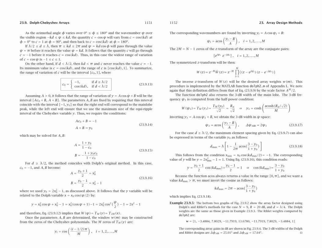
Example 23.9.5: The bottom two graphs of Fig. 23.9.2 show the array factor designed usingDolph’s and Riblet’s methods for the case N = 9, R = 20 dB, and d = λ/4. The Dolphweights are the same as those given in Example 23.9.3. The Riblet weights computed bydolph2 are:

w = [1, −3.4884, 7.8029, −11.7919, 13.6780, −11.7919, 7.8029, −3.4884, 1]

The corresponding array gains in dB are shown in Fig. 23.9.4. The 3-dB widths of the Dolphand Riblet designs are Δφ3dB = 25.01o and Δφ3dB = 17.64o. ��


90o

−90o

0o180o

φ

60o

−60o

30o

−30o

120o

−120o

150o

−150o

−10−20−30dB

Dolph design 90o

−90o

0o180o

φ

60o

−60o

30o

−30o

120o

−120o

150o

−150o

−10−20−30dB

Riblet design

Fig. 23.9.4 Dolph and Riblet designs of Chebyshev array with N = 9, R = 20 dB, d = λ/4.

Next, we discuss steered arrays [1246]. We assume a steering angle 0o < φ0 <180o. The endfire case φ0 = 0o,180o will be treated separately [1247]. The steeredwavenumber will be:

ψ′ = ψ−ψ0 = kd(cosφ− cosφ0) (23.9.19)

where ψ0 = kd cosφ0. The corresponding array weights and array factor will be:

a(m) = e−jmψ0w(m) , −M ≤m ≤MA(ψ) =W(ψ−ψ0)=W(ψ′)= TM(y′), y′ = A cosψ′ + B

(23.9.20)

where we assumed that N is odd, N = 2M + 1. The visible region becomes now:

kd(1− | cosφ0|

) ≤ ψ′ ≤ kd(1+ | cosφ0|)

In order to avoid grating lobes, the element spacing must be less than the maximum:

d0 = λ1+ | cosφ0| (23.9.21)

which satisfies kd0(1+ | cosφ0|

) = 2π.The Chebyshev design method is carried out in the same way, except instead of using

the half-wavelength spacing λ/2 as the dividing line between the Riblet and the Dolphmethods, we must use d0/2. Thus, the variable c = cosψ′ = cos(ψ−ψ0) will vary inthe interval [c0,1], where Eq. (23.9.13) is now replaced by

c0 ={−1, if d ≥ d0/2cos(kd(1+ | cosφ0|)

), if d < d0/2

Replacing 1+ | cosφ0| = λ/d0, we can rewrite this as follows:

c0 =⎧⎪⎨⎪⎩−1, if d ≥ d0/2

cos(2πdd0

), if d < d0/2

(23.9.22)


The solutions for A,B will still be given by Eq. (23.9.15) with this new value for c0.Note that when d < d0/2 the quantities A,B, and hence the array weights w(m), willdepend on φ0. Therefore, the weights must be redesigned for each new value of φ0,instead of simply steering the broadside weights [1246].

When d ≥ d0/2, we have c0 = −1 and the weights w(m) become independent ofφ0. In this case, the steered weights are obtained by steering the broadside weights.

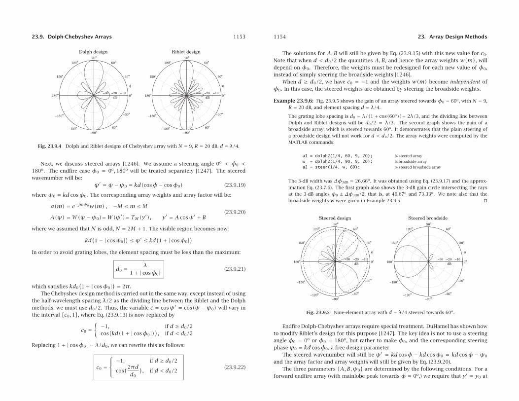
Example 23.9.6: Fig. 23.9.5 shows the gain of an array steered towards φ0 = 60o, with N = 9,R = 20 dB, and element spacing d = λ/4.

The grating lobe spacing is d0 = λ/(1+ cos(60o))= 2λ/3, and the dividing line betweenDolph and Riblet designs will be d0/2 = λ/3. The second graph shows the gain of abroadside array, which is steered towards 60o. It demonstrates that the plain steering ofa broadside design will not work for d < d0/2. The array weights were computed by theMATLAB commands:

a1 = dolph2(1/4, 60, 9, 20); % steered array

w = dolph2(1/4, 90, 9, 20); % broadside array

a2 = steer(1/4, w, 60); % steered broadside array

The 3-dB width was Δφ3dB = 26.66o. It was obtained using Eq. (23.9.17) and the approx-imation Eq. (23.7.6). The first graph also shows the 3-dB gain circle intersecting the raysat the 3-dB angles φ0 ± Δφ3dB/2, that is, at 46.67o and 73.33o. We note also that thebroadside weights w were given in Example 23.9.5. ��

90o

−90o

0o180o

φ

60o

−60o

30o

−30o

120o

−120o

150o

−150o

−10−20−30dB

Steered design 90o

−90o

0o180o

φ

60o

−60o

30o

−30o

120o

−120o

150o

−150o

−10−20−30dB

Steered broadside

Fig. 23.9.5 Nine-element array with d = λ/4 steered towards 60o.

Endfire Dolph-Chebyshev arrays require special treatment. DuHamel has shown howto modify Riblet’s design for this purpose [1247]. The key idea is not to use a steeringangle φ0 = 0o or φ0 = 180o, but rather to make φ0, and the corresponding steeringphase ψ0 = kd cosφ0, a free design parameter.

The steered wavenumber will still be ψ′ = kd cosφ − kd cosφ0 = kd cosφ −ψ0

and the array factor and array weights will still be given by Eq. (23.9.20).The three parameters {A,B,ψ0} are determined by the following conditions. For a

forward endfire array (with mainlobe peak towards φ = 0o,) we require that y′ = y0 at


φ = 0, or, at ψ′ = kd−ψ0. Moreover, we require that the two endpoints y′ = −1 andy′ = 1 of the equi-ripple range of the Chebyshev polynomial are reached at ψ′ = 0 andat φ = 180o, or, ψ′ = −kd−ψ0. These three conditions can be stated as follows:

A cos(kd−ψ0)+B = y0

A+ B = −1

A cos(kd+ψ0)+B = 1

(23.9.23)

For a backward endfire array (with mainlobe towards φ = 180o,) we must replaceψ0 by −ψ0. The solution of Eqs. (23.9.23) is:

A = −y0 + 3+ 2 cos(kd)√

2(y0 + 1)2 sin2(kd)

B = −1−A

ψ0 = ± asin(

y0 − 1

2A sin(kd)

) (23.9.24)

where in the solution forψ0, the plus (minus) sign is chosen for the forward (backward)endfire array. Bidirectional endfire arrays can also be designed. In that case, we setψ0 = 0 and only require the first two conditions in (23.9.23), which become

A cos(kd)+B = y0

A+ B = −1(23.9.25)

with solution:

A = − y0 + 1

1− cos(kd)

B = y0 + cos(kd)1− cos(kd)

(23.9.26)

In all three of the above endfire designs, we must assume d ≤ λ/2 in order to avoidgrating lobes. The MATLAB function dolph3.m of Appendix L implements all threecases.

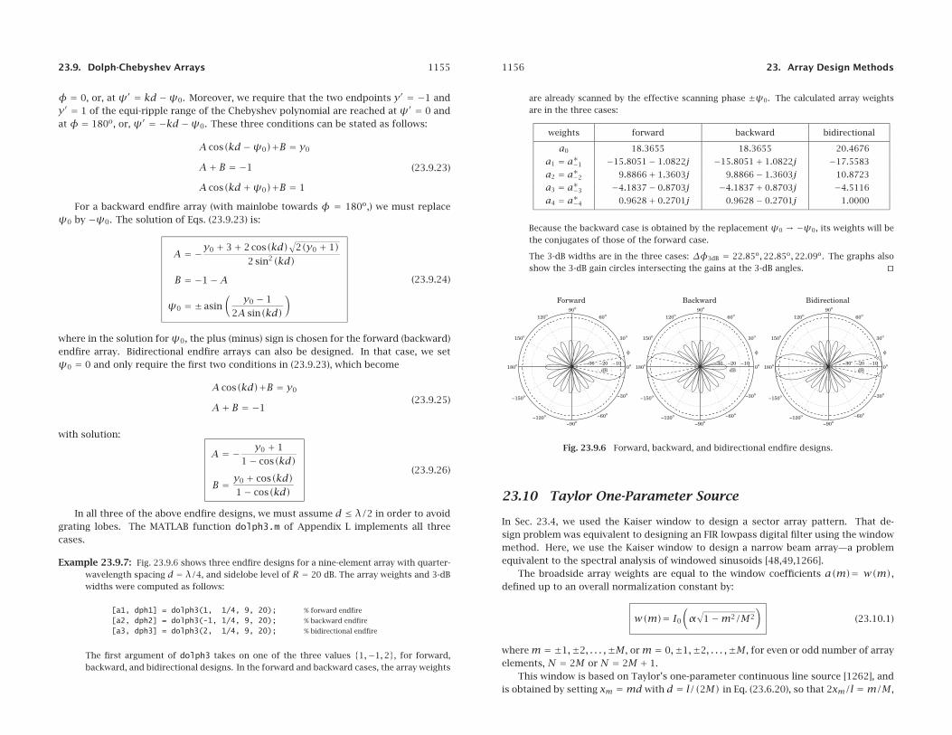
Example 23.9.7: Fig. 23.9.6 shows three endfire designs for a nine-element array with quarter-wavelength spacing d = λ/4, and sidelobe level of R = 20 dB. The array weights and 3-dBwidths were computed as follows:

[a1, dph1] = dolph3(1, 1/4, 9, 20); % forward endfire

[a2, dph2] = dolph3(-1, 1/4, 9, 20); % backward endfire

[a3, dph3] = dolph3(2, 1/4, 9, 20); % bidirectional endfire

The first argument of dolph3 takes on one of the three values {1,−1,2}, for forward,backward, and bidirectional designs. In the forward and backward cases, the array weights


are already scanned by the effective scanning phase ±ψ0. The calculated array weightsare in the three cases:

weights forward backward bidirectional

a0 18.3655 18.3655 20.4676

a1 = a∗−1 −15.8051− 1.0822j −15.8051+ 1.0822j −17.5583

a2 = a∗−2 9.8866+ 1.3603j 9.8866− 1.3603j 10.8723

a3 = a∗−3 −4.1837− 0.8703j −4.1837+ 0.8703j −4.5116

a4 = a∗−4 0.9628+ 0.2701j 0.9628− 0.2701j 1.0000

Because the backward case is obtained by the replacement ψ0 → −ψ0, its weights will bethe conjugates of those of the forward case.

The 3-dB widths are in the three cases: Δφ3dB = 22.85o,22.85o,22.09o. The graphs alsoshow the 3-dB gain circles intersecting the gains at the 3-dB angles. ��

90o

−90o

0o180o

φ

60o

−60o

30o

−30o

120o

−120o

150o

−150o

−10−20−30dB

Forward 90o

−90o

0o180o

φ

60o

−60o

30o

−30o

120o

−120o

150o

−150o

−10−20−30dB

Backward 90o

−90o

0o180o

φ

60o

−60o

30o

−30o

120o

−120o

150o

−150o

−10−20−30dB

Bidirectional

Fig. 23.9.6 Forward, backward, and bidirectional endfire designs.

23.10 Taylor One-Parameter Source

In Sec. 23.4, we used the Kaiser window to design a sector array pattern. That de-sign problem was equivalent to designing an FIR lowpass digital filter using the windowmethod. Here, we use the Kaiser window to design a narrow beam array—a problemequivalent to the spectral analysis of windowed sinusoids [48,49,1266].

The broadside array weights are equal to the window coefficients a(m)= w(m),defined up to an overall normalization constant by:

w(m)= I0(α√

1−m2/M2

)(23.10.1)

wherem = ±1,±2, . . . ,±M, orm = 0,±1,±2, . . . ,±M, for even or odd number of arrayelements, N = 2M or N = 2M + 1.

This window is based on Taylor’s one-parameter continuous line source [1262], andis obtained by setting xm =md with d = l/(2M) in Eq. (23.6.20), so that 2xm/l =m/M,

23.10. Taylor One-Parameter Source 1157

I(xm)= I0(πB√

1− (2xm/l)2

)= I0

(πB√

1− (m/M)2

)

Thus, we note that the Kaiser window shape parameter α is related to Taylor’s pa-rameter B by α = πB. The parameter B or α control the sidelobe level. The continuousline pattern of (23.6.20),

F(u)=sinh

(π√B2 − u2

)π√B2 − u2

=sin(π√u2 − B2

)π√u2 − B2

(23.10.2)

has a first null at u0 =√B2 + 1, and therefore, the first sidelobe will occur for u > u0.

For this range, we must use the sinc-form of F(u) and to find the maximum sidelobelevel, we must find the maximum of the sinc function (for argument other than zero).This can be determined, for example, by the MATLAB command:†

x0=fminbnd(’sinc(x)’, 1,2, optimset(’TolX’,eps)); r0 = abs(sinc(x0));

which yields the values:

x0 = 1.4302966532

r0 =∣∣sinc(x0)

∣∣ = 0.2172336282

R0 = −20 log10(r0)= 13.2614588840 dB

(23.10.3)

The sidelobe levelRa (in absolute units) is defined as the ratio of the pattern at u = 0to the maximum sidelobe level r0, that is,

Ra = 1

r0

sinh(πB)πB

(23.10.4)

and in dB, R = 20 log10(Ra),

R = R0 + 20 log10

(sinh(πB)πB

)(23.10.5)

To avoid having to solve (23.10.4) for B for a given Ra, Kaiser and Schafer [1266]have developed an empirical formula in terms of the sidelobe level R in dB, which isvalid across the range 13 < R < 120 dB:

πB =

⎧⎪⎪⎨⎪⎪⎩

0, R ≤ 13.26

0.76609(R− 13.26)0.4+0.09834(R− 13.26), 13.26<R≤ 60

0.12438(R+ 6.3), 60<R< 120

(23.10.6)

For R ≤ 13.26, w(m) becomes the rectangular window. The broadening factor b,and the 3-dB width in ψ-space can also be expressed in terms of the dB sidelobe levelR by the following empirical formula valid for 20 < R < 100 dB:

b = 0.01330R+ 0.9761 , Δψ3dB = 0.8862πbN

(23.10.7)

†MATLAB’s sinc function is defined as sinc(x)= sinπx/πx.


The 3-dB width in angle space, Δφ3dB, is then calculated from Eq. (23.7.6). The 3-dBbeam width may be more accurately calculated by finding it in u-space, say Δu, andthen transforming it to ψ-space using Eq. (23.6.15), Δψ3dB = 2πΔu/N. The width Δuis given by Δu = 2u3, where u3 is the solution of the half-power condition:

∣∣F(u3)∣∣2 = 1

2

∣∣F(0)∣∣2 ⇒sinh

(π√B2 − u2

3

)

π√B2 − u2

3

= 1√2

sinh(πB)πB

(23.10.8)

For small values of B, the right-hand side becomes less than one, and we must switchthe left-hand side to its sinc form. This happens when B ≤ Bc, where

1√2

sinh(πBc)πBc

= 1 ⇒ Bc = 0.4747380492 (23.10.9)

which, through (23.10.5), corresponds to a sidelobe attenuation ofRc = 16.27 dB. Ratherthan using the above empirical formulas, Eqs. (23.10.4) and (23.10.8) may be solvednumerically in MATLAB. The function taylorbw implements the solution, returning thevalues of B and Δu, for any vector of sidelobe attenuations R:

[B,Du] = taylorbw(R); % Taylor parameter B and beamwidth Δu

It is built on the functions sinhc and asinhc for computing the hyperbolic sincfunction and its inverse:

y = sinhc(x); % hyperbolic sinc function, sinhc(x) = sinh(π x)/π x

x = asinhc(y); % inverse function, finds the x that satisfies sinhc(x) = y

For small x, the equation y = sinh(x)/x is solved for x by using the Taylor seriesexpansion y = sinh(x)x � 1 + x2/6 + x4/120; for larger x, it is solved by the iterationsinh(xn)/xn−1 = y, or, xn = asinh(yxn−1), for n = 1,2, . . . .

Once the B-parameter is determined, the array weightsw(m) can be computed from(23.10.1) using the built-in function besseli, and then steered towards an angle φ0

using Eq. (23.7.1). In this case, to avoid grating lobes, the element spacing must be lessthan the maximum:

d0 = λ1+ | cosφ0| (23.10.10)

As discussed in Sec. 23.9, in order for the visible region is ψ-space to cover at leastone Nyquist period, the element spacing d must be in the range:

d0

2≤ d < d0 (23.10.11)

The MATLAB function taylor1p of Appendix L implements this design procedureand invokes the function taylorbw. The outputs of the function are the steered arrayweights and the 3-dB width. It has usage:

[a, dph] = taylor1p(d, ph0, N, R); % Taylor 1-parameter line source

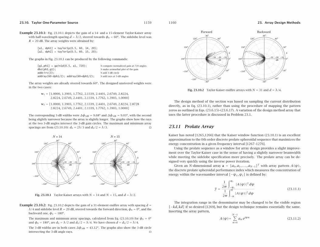
23.10. Taylor One-Parameter Source 1159

Example 23.10.1: Fig. 23.10.1 depicts the gain of a 14- and a 15-element Taylor-Kaiser arraywith half-wavelength spacing d = λ/2, steered towards φ0 = 60o. The sidelobe level wasR = 20 dB. The array weights were obtained by:

[a1, dph1] = taylor1p(0.5, 60, 14, 20);[a2, dph2] = taylor1p(0.5, 60, 15, 20);

The graphs in Fig. 23.10.1 can be produced by the following commands:

[g1,ph1] = gain1d(0.5, a1, 720); % compute normalized gain at 720 angles

dbz(ph1,g1); % make azimuthal plot of the gain

addcirc(3); % add 3-dB circle

addray(60-dph1/2); addray(60+dph1/2); % add rays at 3-dB angles

The array weights are already steered towards 60o. The designed unsteered weights werein the two cases:

w1 = [1.0000, 1.3903, 1.7762, 2.1339, 2.4401, 2.6749, 2.8224,2.8224, 2.6749, 2.4401, 2.1339, 1.7762, 1.3903, 1.0000]

w2 = [1.0000, 1.3903, 1.7762, 2.1339, 2.4401, 2.6749, 2.8224, 2.87282.8224, 2.6749, 2.4401, 2.1339, 1.7762, 1.3903, 1.0000]

The corresponding 3-dB widths were Δφ3dB = 9.68o and Δφ3dB = 9.03o, with the secondbeing slightly narrower because the array is slightly longer. The graphs show how the raysat the two 3-dB angles intersect the 3-dB gain circles. The maximum and minimum arrayspacings are from (23.10.10): d0 = 2λ/3 and d0/2 = λ/3. ��

90o

−90o

0o180o

φ

60o

−60o

30o

−30o

120o

−120o

150o

−150o

−10−20−30dB

N = 14 90o

−90o

0o180o

φ

60o

−60o

30o

−30o

120o

−120o

150o

−150o

−10−20−30dB

N = 15

Fig. 23.10.1 Taylor-Kaiser arrays with N = 14 and N = 15, and d = λ/2.

Example 23.10.2: Fig. 23.10.2 depicts the gain of a 31-element endfire array with spacing d =λ/4 and sidelobe level R = 20 dB, steered towards the forward direction,φ0 = 0o, and thebackward one, φ0 = 180o.

The maximum and minimum array spacings, calculated from Eq. (23.10.10) for φ0 = 0o

and φ0 = 180o, are d0 = λ/2 and d0/2 = λ/4. We have chosen d = d0/2 = λ/4.

The 3-dB widths are in both cases Δφ3dB = 43.12o. The graphs also show the 3-dB circleintersecting the 3-dB angle rays. ��


90o

−90o

0o180o

φ

60o

−60o

30o

−30o

120o

−120o

150o

−150o

−10−20−30dB

Forward 90o

−90o

0o180o

φ

60o

−60o

30o

−30o

120o

−120o

150o

−150o

−10−20−30dB

Backward

Fig. 23.10.2 Taylor-Kaiser endfire arrays with N = 31 and d = λ/4.

The design method of the section was based on sampling the current distributiondirectly, as in Eq. (23.10.1), rather than using the procedure of mapping the patternzeros as outlined in Eqs. (23.6.15)–(23.6.17). A variation of the design method array thatuses the latter procedure is discussed in Problem 23.1.

23.11 Prolate Array

Kaiser has noted [1265,1266] that the Kaiser window function (23.10.1) is an excellentapproximation to the 0th order discrete prolate spheroidal sequence that maximizes theenergy concentration in a given frequency interval [1267–1276].

Using the prolate sequence as a window for array design provides a slight improve-ment over the Taylor-Kaiser case in the sense of having a slightly narrower beamwidthwhile meeting the sidelobe specification more precisely. The prolate array can be de-signed very quickly using the inverse power iteration.

Given an N-dimensional array a = [a0, a1, . . . , aN−1]T with array pattern A(ψ),the discrete prolate spheroidal performance index which measures the concentration ofenergy within the wavenumber interval [−ψc,ψc] is defined by:

J =1

2π

∫ ψc−ψc

|A(ψ)|2 dψ1

2π

∫ π−π|A(ψ)|2 dψ

(23.11.1)

The integration range in the denominator may be changed to be the visible region[−kd, kd] if so desired [1269], but the design technique remains essentially the same.Inserting the array pattern,

A(ψ)=N−1∑n=0

an ejψn (23.11.2)

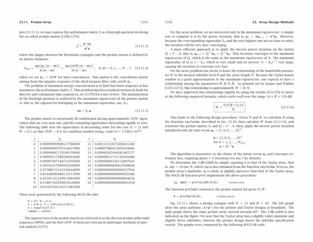
23.11. Prolate Array 1161

into (23.11.1), we may express the performance index J as a Rayleigh quotient involvingthe so-called prolate matrix [1268,1276]:

J = a†Aa

a†a(23.11.3)

where the dagger denotes the Hermitian conjugate and the prolate matrix is defined byits matrix elements:

Anm = sin(ψc(n−m)

)π(n−m) = sin

(2πW(n−m))π(n−m) , n,m = 0,1, . . . ,N − 1 (23.11.4)

where we set ψc = 2πW for later convenience. This matrix is the convolution matrixarising from the impulse response of the ideal lowpass filter with cutoff ψc.

The problem of maximum energy concentration is to find that finite sequence a thatmaximizes the performance indexJ. This problem has been studied extensively both fordiscrete and continuous time sequences, see [1270] for a nice review. The maximizationof the Rayleigh quotient is realized by the maximum eigenvector of the prolate matrixA, that is, the eigenvector belonging to the maximum eigenvalue, say, λ0:

Aa = λ0 a (23.11.5)

The prolate matrix is notoriously ill-conditioned having approximately 2NW eigen-values that are very near one, and the remaining eigenvalues decreasing rapidly to zero.The following table lists the eigenvalues in decreasing order for the case N = 21 andW = 0.2, so that 2NW = 8.4, its condition number being, cond(A)= 5.1063×1016:

i λi0 0.999999999985177860001 0.999999997955146270002 0.999999871705401390003 0.999995173885083630004 0.999879471497147950005 0.997924570999562000006 0.975881221455426440007 0.834460904801197170008 0.455911422409130630009 0.11887181858959120000

10 0.01567636516215985600

i λi11 0.0013155267149002150012 0.0000798691560561804613 0.0000036549438148257714 0.0000001273114920448615 0.0000000033615409764316 0.0000000000662166866817 0.0000000000009432794418 0.0000000000000092018619 0.0000000000000000403420 0.00000000000000001958

These were generated by the following MATLAB code:

N = 21; W = 0.2;n = 0:N-1; f = 2*W*sinc(2*W*n);A = toeplitz(f,f);lambda = svd(A);

The eigenvectors of the prolate matrix are referred to as the discrete prolate spheroidalsequences (DPSS), and the first 2NW of them are relevant in multitaper methods of spec-tral analysis [1275] .


For the array problem, we are interested only in the maximum eigenvector. A simpleway to compute it is by the power iteration, that is, an = Aan−1 = Ana0. However,because the corresponding eigenvalue λ0 and the next highest one are so close to unity,the iteration will be very slow converging.

A more efficient approach is to apply the inverse power iteration on the matrixQ = I − A, that is, an+1 = Q−1an = Q−na0. This iteration converges to the minimumeigenvector of Q, which is the same as the maximum eigenvector of A. The minimumeigenvalue of Q is 1 − λ0, which is very small and its inverse (1 − λ0)−1 very large,causing the iteration to converge very fast.

For the array problem one needs to know the relationship of the bandwidth parame-terW to the desired sidelobe level R and the array length N. Because the Taylor-Kaiserwindow is a good approximation to the maximum eigenvector, one expects to have arelationship among the parameters W,B,N,R. As pointed out by Kaiser and Walden[1265,1272], this relationship is approximatelyW = B/N.

We have improved this relationship slightly by using the results of [1276] to arriveat the following empirical formula, which works well over the range 14 ≤ R ≤ 120 dB:

W = 0.95B+ 0.14

N(23.11.6)

This leads to the following design procedure. Given N and R, we calculate B usingthe function taylorbw, described in Sec. 23.10, then calculate W from (23.11.6), andconstruct the prolate matrix A, and Q = I −A, then, apply the inverse power iterationinitialized with the unit vector a0 = [1,0,0, . . . ,0]T:

a = [1,0,0, . . . ,0]Tfor n = 1,2, . . . ,Niter,

a = Q−1a

The algorithm is insensitive to the choice of the initial vector a0 and converges ex-tremely fast, requiring about 1–3 iterations (we use 3 by default).

We determine the 3-dB width by simply equating it to that of the Taylor array, thatis, Δψ = 2πΔu/N, whereΔu is also obtained from the function taylorbw. Even so, theprolate array’s mainlobe, as a whole, is slightly narrower than that of the Taylor array.The MATLAB function prol implements the above procedure:

[a, dph] = prol(d,ph0,N,R); % prolate array

The function prolmat constructs the prolate matrix for given N,W:

A = prolmat(N,W); % prolate matrix

Fig. 23.11.1 shows a design example with N = 21 and R = 30. The left graphplots the array patterns |A(ψ)| for the prolate and Taylor designs at broadside. Theright graph shows the same prolate array steered towards 60o. The 3-dB width is alsoindicated on the figure. We note that the Taylor array has a slightly wider mainlobe andslightly lower sidelobes, whereas the prolate design meets the sidelobe specificationexactly. The graphs were computed by the following MATLAB code:

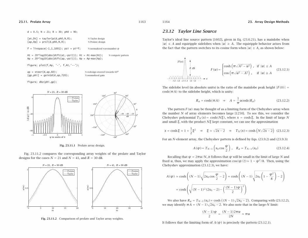
23.11. Prolate Array 1163

d = 0.5; N = 21; R = 30; ph0 = 90;

[at,Dt] = taylor1p(d,ph0,N,R); % Taylor design

[ap,Dp] = prol(d,ph0,N,R); % Prolate design

f = linspace(-1,1,1001); psi = pi*f; % normalized wavenumber ψ

At = 20*log10(abs(dtft(at,-psi))); At = At-max(At); % compute pattern

Ap = 20*log10(abs(dtft(ap,-psi))); Ap = Ap-max(Ap);

figure; plot(f,Ap, ’-’, f,At,’--’);

ap = steer(d,ap,60); % redesign steered towards 60o

[gp,phi] = gain1d(d,ap,720); % normalized gain

figure; dbz(phi,gp);

−1 −0.5 0 0.5 1

−60

−30

0

ψ in units of π

|A

(ψ)|

in d

B

N = 21, R = 30 dB

ProlateTaylor

90o

−90o

0o180o

φ

60o

−60o

30o

−30o

120o

−120o

150o

−150o

−10−20−30dB

Fig. 23.11.1 Prolate array design.

Fig. 23.11.2 compares the corresponding array weights of the prolate and Taylordesigns for the cases N = 21 and N = 41, and R = 30 dB.

0 5 10 15 200

0.5

1

m

a(m

)

N = 21, R = 30 dB

ProlateTaylor

0 10 20 30 400

0.5

1

m

a(m

)

N = 41, R = 30 dB

ProlateTaylor

Fig. 23.11.2 Comparison of prolate and Taylor array weights.


23.12 Taylor Line Source

Taylor’s ideal line source pattern [1602], given in Eq. (23.6.21), has a mainlobe when|u| ≤ A and equiripple sidelobes when |u| ≥ A. The equiripple behavior arises fromthe fact that the pattern switches to its cosine form when |u| ≥ A, as shown below:

F(u)=⎧⎪⎨⎪⎩

cosh(π√A2 − u2

), if |u| ≤ A

cos(π√u2 −A2

), if |u| ≥ A

(23.12.1)

The sidelobe level (in absolute units) is the ratio of the mainlobe peak height |F(0)| =cosh(πA) to the sidelobe height, which is unity:

Ra = cosh(πA) ⇒ A = 1

πacosh(Ra) (23.12.2)

The pattern F(u)may be thought of as a limiting form of the Chebyshev array whenthe number N of array elements becomes large [1250]. To see this, we consider theChebyshev polynomial TN(x)= cosh(Nξ), where x = coshξ. In the limit of large Nand small ξ, with the product Nξ kept constant, we can use the approximation

x = coshξ � 1+ 1

2ξ2 ⇒ ξ � √2x− 2 ⇒ TN(x)� cosh

(N√

2x− 2)

(23.12.3)

For an N-element array, the Chebyshev pattern is defined by Eqs. (23.9.2) and (23.9.3):

A(ψ)= TN−1

(x0 cos

ψ2

), Ra = TN−1(x0) (23.12.4)

Recalling thatψ = 2πu/N, it follows thatψ will be small in the limit of largeN andfixed u, thus, we may apply the approximation cos(ψ/2)� 1 −ψ2/8. Then, using theChebyshev approximation (23.12.3), we have:

A(ψ) � cosh

((N − 1)

√2x0 cos

ψ2− 2

)= cosh

⎛⎝(N − 1)

√√√√2x0

(1− ψ

2

8

)− 2

⎞⎠

= cosh

⎛⎝√(N − 1)2(2x0 − 2)−

((N − 1)ψ

2

)2⎞⎠

We also have Ra = TN−1(x0)� cosh((N − 1)

√2x0 − 2

). Comparing with (23.12.2),

we may identify πA = (N − 1)√

2x0 − 2. We also note that in the large-N limit:

(N − 1)ψ2

= (N − 1)2πu2N

� πu

It follows that the limiting form of A(ψ) is precisely the pattern (23.12.1).

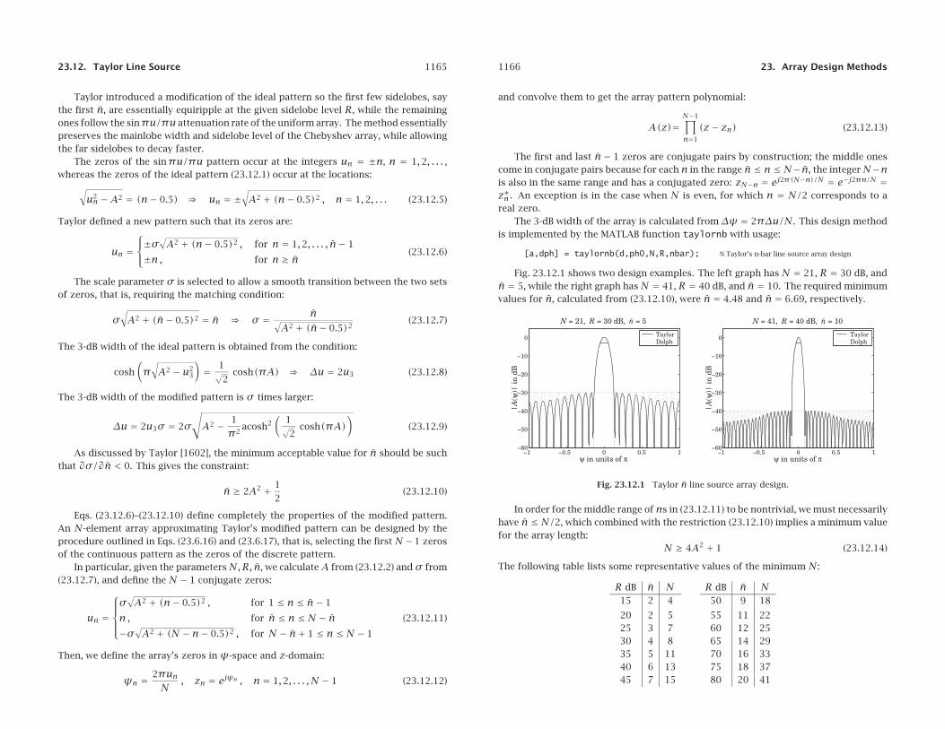
23.12. Taylor Line Source 1165

Taylor introduced a modification of the ideal pattern so the first few sidelobes, saythe first n, are essentially equiripple at the given sidelobe level R, while the remainingones follow the sinπu/πu attenuation rate of the uniform array. The method essentiallypreserves the mainlobe width and sidelobe level of the Chebyshev array, while allowingthe far sidelobes to decay faster.

The zeros of the sinπu/πu pattern occur at the integers un = ±n, n = 1,2, . . . ,whereas the zeros of the ideal pattern (23.12.1) occur at the locations:√

u2n −A2 = (n− 0.5) ⇒ un = ±

√A2 + (n− 0.5)2 , n = 1,2, . . . (23.12.5)

Taylor defined a new pattern such that its zeros are:

un =⎧⎨⎩±σ

√A2 + (n− 0.5)2 , for n = 1,2, . . . , n− 1

±n , for n ≥ n (23.12.6)

The scale parameter σ is selected to allow a smooth transition between the two setsof zeros, that is, requiring the matching condition:

σ√A2 + (n− 0.5)2 = n ⇒ σ = n√

A2 + (n− 0.5)2(23.12.7)

The 3-dB width of the ideal pattern is obtained from the condition:

cosh(π√A2 − u2

3

)= 1√

2cosh(πA) ⇒ Δu = 2u3 (23.12.8)

The 3-dB width of the modified pattern is σ times larger:

Δu = 2u3σ = 2σ

√A2 − 1

π2acosh2

(1√2

cosh(πA))

(23.12.9)

As discussed by Taylor [1602], the minimum acceptable value for n should be suchthat ∂σ/∂n < 0. This gives the constraint:

n ≥ 2A2 + 1

2(23.12.10)

Eqs. (23.12.6)–(23.12.10) define completely the properties of the modified pattern.An N-element array approximating Taylor’s modified pattern can be designed by theprocedure outlined in Eqs. (23.6.16) and (23.6.17), that is, selecting the firstN−1 zerosof the continuous pattern as the zeros of the discrete pattern.

In particular, given the parametersN,R, n, we calculateA from (23.12.2) andσ from(23.12.7), and define the N − 1 conjugate zeros:

un =

⎧⎪⎪⎨⎪⎪⎩σ√A2 + (n− 0.5)2 , for 1 ≤ n ≤ n− 1

n , for n ≤ n ≤ N − n−σ√A2 + (N − n− 0.5)2 , for N − n+ 1 ≤ n ≤ N − 1

(23.12.11)

Then, we define the array’s zeros in ψ-space and z-domain:

ψn = 2πunN

, zn = ejψn , n = 1,2, . . . ,N − 1 (23.12.12)


and convolve them to get the array pattern polynomial:

A(z)=N−1∏n=1

(z− zn) (23.12.13)

The first and last n − 1 zeros are conjugate pairs by construction; the middle onescome in conjugate pairs because for each n in the range n ≤ n ≤ N−n, the integerN−nis also in the same range and has a conjugated zero: zN−n = ej2π(N−n)/N = e−j2πn/N =z∗n . An exception is in the case when N is even, for which n = N/2 corresponds to areal zero.

The 3-dB width of the array is calculated from Δψ = 2πΔu/N. This design methodis implemented by the MATLAB function taylornb with usage:

[a,dph] = taylornb(d,ph0,N,R,nbar); % Taylor’s n-bar line source array design

Fig. 23.12.1 shows two design examples. The left graph has N = 21, R = 30 dB, andn = 5, while the right graph hasN = 41, R = 40 dB, and n = 10. The required minimumvalues for n, calculated from (23.12.10), were n = 4.48 and n = 6.69, respectively.

−1 −0.5 0 0.5 1−60

−50

−40

−30

−20

−10

0

ψ in units of π

|A

(ψ)|

in d

B

N = 21, R = 30 dB, n = 5

TaylorDolph

−1 −0.5 0 0.5 1−60

−50

−40

−30

−20

−10

0

ψ in units of π

|A

(ψ)|

in d

B

N = 41, R = 40 dB, n = 10

TaylorDolph

Fig. 23.12.1 Taylor n line source array design.

In order for the middle range of ns in (23.12.11) to be nontrivial, we must necessarilyhave n ≤ N/2, which combined with the restriction (23.12.10) implies a minimum valuefor the array length:

N ≥ 4A2 + 1 (23.12.14)

The following table lists some representative values of the minimum N:

R dB n N15 2 4

20 2 525 3 730 4 835 5 1140 6 1345 7 15

R dB n N50 9 18

55 11 2260 12 2565 14 2970 16 3375 18 3780 20 41

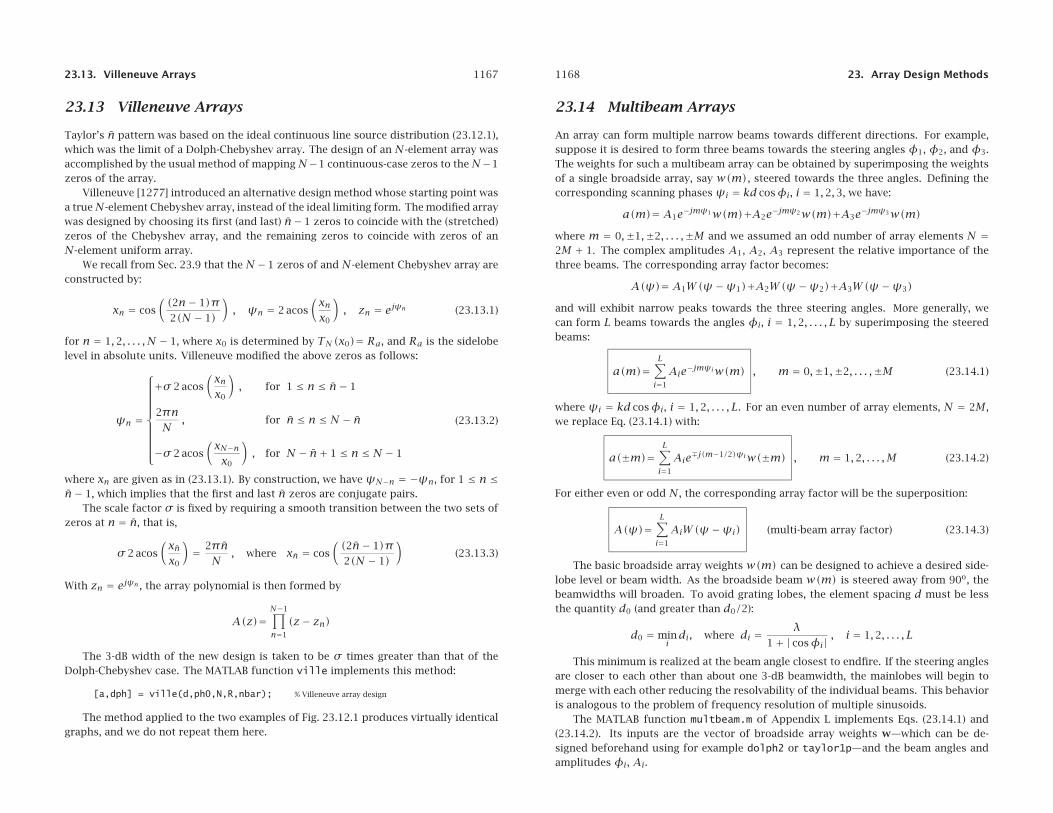
23.13. Villeneuve Arrays 1167

23.13 Villeneuve Arrays

Taylor’s n pattern was based on the ideal continuous line source distribution (23.12.1),which was the limit of a Dolph-Chebyshev array. The design of an N-element array wasaccomplished by the usual method of mappingN−1 continuous-case zeros to theN−1zeros of the array.

Villeneuve [1277] introduced an alternative design method whose starting point wasa trueN-element Chebyshev array, instead of the ideal limiting form. The modified arraywas designed by choosing its first (and last) n− 1 zeros to coincide with the (stretched)zeros of the Chebyshev array, and the remaining zeros to coincide with zeros of anN-element uniform array.

We recall from Sec. 23.9 that the N−1 zeros of and N-element Chebyshev array areconstructed by:

xn = cos((2n− 1)π2(N − 1)

), ψn = 2 acos

(xnx0

), zn = ejψn (23.13.1)

for n = 1,2, . . . ,N − 1, where x0 is determined by TN(x0)= Ra, and Ra is the sidelobelevel in absolute units. Villeneuve modified the above zeros as follows:

ψn =

⎧⎪⎪⎪⎪⎪⎪⎪⎪⎪⎨⎪⎪⎪⎪⎪⎪⎪⎪⎪⎩

+σ 2 acos(xnx0

), for 1 ≤ n ≤ n− 1

2πnN, for n ≤ n ≤ N − n

−σ 2 acos(xN−nx0

), for N − n+ 1 ≤ n ≤ N − 1

(23.13.2)

where xn are given as in (23.13.1). By construction, we have ψN−n = −ψn, for 1 ≤ n ≤n− 1, which implies that the first and last n zeros are conjugate pairs.

The scale factor σ is fixed by requiring a smooth transition between the two sets ofzeros at n = n, that is,

σ 2 acos(xnx0

)= 2πnN, where xn = cos

((2n− 1)π2(N − 1)

)(23.13.3)

With zn = ejψn , the array polynomial is then formed by

A(z)=N−1∏n=1

(z− zn)

The 3-dB width of the new design is taken to be σ times greater than that of theDolph-Chebyshev case. The MATLAB function ville implements this method:

[a,dph] = ville(d,ph0,N,R,nbar); % Villeneuve array design

The method applied to the two examples of Fig. 23.12.1 produces virtually identicalgraphs, and we do not repeat them here.


23.14 Multibeam Arrays

An array can form multiple narrow beams towards different directions. For example,suppose it is desired to form three beams towards the steering angles φ1, φ2, and φ3.The weights for such a multibeam array can be obtained by superimposing the weightsof a single broadside array, say w(m), steered towards the three angles. Defining thecorresponding scanning phases ψi = kd cosφi, i = 1,2,3, we have:

a(m)= A1e−jmψ1w(m)+A2e−jmψ2w(m)+A3e−jmψ3w(m)

where m = 0,±1,±2, . . . ,±M and we assumed an odd number of array elements N =2M + 1. The complex amplitudes A1, A2, A3 represent the relative importance of thethree beams. The corresponding array factor becomes:

A(ψ)= A1W(ψ−ψ1)+A2W(ψ−ψ2)+A3W(ψ−ψ3)

and will exhibit narrow peaks towards the three steering angles. More generally, wecan form L beams towards the angles φi, i = 1,2, . . . , L by superimposing the steeredbeams:

a(m)=L∑i=1

Aie−jmψiw(m) , m = 0,±1,±2, . . . ,±M (23.14.1)

where ψi = kd cosφi, i = 1,2, . . . , L. For an even number of array elements, N = 2M,we replace Eq. (23.14.1) with:

a(±m)=L∑i=1

Aie∓j(m−1/2)ψiw(±m) , m = 1,2, . . . ,M (23.14.2)

For either even or odd N, the corresponding array factor will be the superposition:

A(ψ)=L∑i=1

AiW(ψ−ψi) (multi-beam array factor) (23.14.3)

The basic broadside array weights w(m) can be designed to achieve a desired side-lobe level or beam width. As the broadside beam w(m) is steered away from 90o, thebeamwidths will broaden. To avoid grating lobes, the element spacing d must be lessthe quantity d0 (and greater than d0/2):

d0 = minidi, where di = λ

1+ | cosφi| , i = 1,2, . . . , L

This minimum is realized at the beam angle closest to endfire. If the steering anglesare closer to each other than about one 3-dB beamwidth, the mainlobes will begin tomerge with each other reducing the resolvability of the individual beams. This behavioris analogous to the problem of frequency resolution of multiple sinusoids.

The MATLAB function multbeam.m of Appendix L implements Eqs. (23.14.1) and(23.14.2). Its inputs are the vector of broadside array weights w—which can be de-signed beforehand using for example dolph2 or taylor1p—and the beam angles andamplitudes φi, Ai.

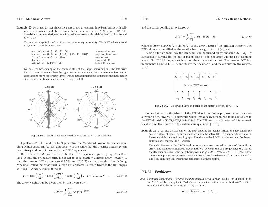
23.14. Multibeam Arrays 1169

Example 23.14.1: Fig. 23.14.1 shows the gains of two 21-element three-beam arrays with half-wavelength spacing, and steered towards the three angles of 45o, 90o, and 120o. Thebroadside array was designed as a Taylor-Kaiser array with sidelobe level of R = 20 andR = 30 dB.

The relative amplitudes of the three beams were equal to unity. The MATLAB code usedto generate the right figure was:

w = taylor1p(0.5, 90, 21, 30); % unsteered weights

a = multbeam(0.5, w, [1,1,1], [45, 90, 120]); % equal-amplitude beams

[g, ph] = array(d, a, 400); % compute gain

dbz(ph, g); % plot gain in dB

addray(45); addray(-45); % add ± 45o grid rays

We note the broadening of the beam widths of the larger beam angles. The left arrayhas narrower mainlobes than the right one because its sidelobe attenuation is less. But, italso exhibits more constructive interference between mainlobes causing somewhat smallersidelobe attenuations than the desired one of 20 dB. ��

90o

−90o

0o180o

φ

60o

−60o

30o

−30o

120o

−120o

150o

−150o

−10−20−30dB

R = 20 dB 90o

−90o

0o180o

φ

60o

−60o

30o

−30o

120o

−120o

150o

−150o

−10−20−30dB

R = 30 dB

Fig. 23.14.1 Multi-beam arrays with R = 20 and R = 30 dB sidelobes.

Equations (23.14.1) and (23.14.2) generalize the Woodward-Lawson frequency sam-pling design equations (23.5.6) and (23.5.7) in the sense that the steering phasesψi canbe arbitrary and do not have to be the DFT frequencies.

However, if the ψi are chosen to be the DFT frequencies given by Eq. (23.5.1) or(23.5.5), and the broadside array is chosen to be a length-N uniform array, w(m)= 1,then the inverse DFT expressions (23.5.6) and (23.5.7) can be thought of as definingN beams—called the Woodward-Lawson-Butler beams—steered towards the DFT anglesφi = acos(ψi/kd), that is, towards

φi = acos(ψikd

)= acos

(2πiNkd

)= acos

(λiNd

), i = 0,1, . . . ,N − 1 (23.14.4)

The array weights will be given then by the inverse DFT:

a(m)= 1

N

N−1∑i=0

A(ψi)e−jmψi (23.14.5)


and the corresponding array factor by:

A(ψ)= 1

N

N−1∑i=0

A(ψi)W(ψ−ψi) (23.14.6)

where W(ψ)= sin(Nψ/2)/ sin(ψ/2) is the array factor of the uniform window. TheDFT values are identified as the relative beam weights Ai = A(ψi)/N.

A single Butler beam, say the jth beam, can be turned on by choosing Ai = δij. Bysuccessively turning on the Butler beams one by one, the array will act as a scanningarray. Fig. 23.14.2 depicts such a multi-beam array structure. The inverse DFT boximplements Eq. (23.14.5). The inputs are the “beams”Ai and the outputs are the weightsa(m).

Fig. 23.14.2 Woodward-Lawson-Butler beam matrix network for N = 8.

Somewhat before the advent of the FFT algorithm, Butler proposed a hardware re-alization of the inverse DFT network, which was quickly recognized to be equivalent tothe FFT algorithm [1278,1279,1281–1284]. The DFT matrix realization of this networkis called the Blass matrix in the antenna array context [18,10].

Example 23.14.2: Fig. 23.14.3 shows the individual Butler beams turned on successively foran eight-element array. Both the standard and alternative DFT frequency sets are shown.There are eight beams in each graph. For the standard DFT set, the two endfire beamscount as one, that is, the i = 0 beam.

The sidelobes are at the 13-dB level because these are scanned versions of the uniformarray. The mainlobes intersect exactly half-way between the DFT frequencies ψi, that is,the ith beam intersects the neighboring ones at ψ = ψi +π/N = 2π(i + 0.5)/N. Theseintersection points are approximately 4 dB down (3.92 dB to be exact) from the main peaks.The 4-dB gain circle intersects the gain curves at these points. ��

23.15 Problems

23.1 Computer Experiment—Taylor’s one-parameter/n array design. Taylor’s n distribution ofSec. 23.12 can also be applied to Taylor’s one-parameter continuous distribution of Sec. 23.10.First, show that the zeros of Eq. (23.10.2) occur at

un =√B2 + n2 , n = 1,2, . . .

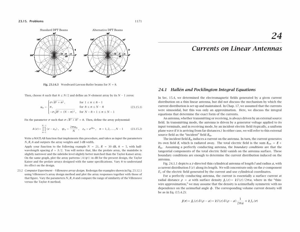
23.15. Problems 1171

90o

−90o

0o180o

φ

45o

−45o

135o

−135o

−4−8−12dB

90o

−90o

0o180o

φ

45o

−45o

135o

−135o

−4−8−12dB

90o

−90o

0o180o

φ

45o

−45o

135o

−135o

−4−8−12dB

90o

−90o

0o180o

φ

45o

−45o

135o

−135o

−4−8−12dB

90o

−90o

0o180o

φ

45o

−45o

135o

−135o

−4−8−12dB

90o

−90o

0o180o

φ

45o

−45o

135o

−135o

−4−8−12dB

90o

−90o

0o180o

φ

45o

−45o

135o

−135o

−4−8−12dB

90o

−90o

0o180o

φ

45o

−45o

135o

−135o

−4−8−12dB

Standard DFT Beams 90o

−90o

0o180o

φ

45o

−45o

135o

−135o

−4−8−12dB

90o

−90o

0o180o

φ

45o

−45o

135o

−135o

−4−8−12dB

90o

−90o

0o180o

φ

45o

−45o

135o

−135o

−4−8−12dB

90o

−90o

0o180o

φ

45o

−45o

135o

−135o

−4−8−12dB

90o

−90o

0o180o

φ

45o

−45o

135o

−135o

−4−8−12dB

90o

−90o

0o180o

φ

45o

−45o

135o

−135o

−4−8−12dB

90o

−90o

0o180o

φ

45o

−45o

135o

−135o

−4−8−12dB

90o

−90o

0o180o

φ

45o

−45o

135o

−135o

−4−8−12dB

Alternative DFT Beams

Fig. 23.14.3 Woodward-Lawson-Butler beams for N = 8.

Then, choose n such that n ≤ N/2 and define an N-element array by its N − 1 zeros:

un =

⎧⎪⎪⎪⎨⎪⎪⎪⎩σ√B2 + n2 , for 1 ≤ n ≤ n− 1

n , for n ≤ n ≤ N − n−σ

√B2 + (N − n)2 , for N − n+ 1 ≤ n ≤ N − 1

(23.15.1)

Fix the parameter σ such that σ√B2 + n2 = n. Then, define the array polynomial:

A(z)=N−1∏n=1

(z− zn) , ψn = 2πunN

, zn = ejψn , n = 1,2, . . . ,N − 1 (23.15.2)

Write a MATLAB function that implements this procedure, and takes as input the parametersN,R, n and outputs the array weights and 3-dB width.

Apply your function to the following example N = 21, R = 30 dB, n = 5, with half-wavelength spacing d = λ/2. You will notice that, like the prolate array, the mainlobe isslightly narrower and the sidelobe level slightly better matched than the Taylor-Kaiser array.On the same graph, plot the array patterns |A(ψ)| in dB for the present design, the TaylorKaiser and the prolate arrays designed with the same specifications. Vary n to understandits effect on the design.

23.2 Computer Experiment—Villeneuve array design. Redesign the examples shown in Fig. 23.12.1using Villeneuve’s array design method and plot the array responses together with those ofthat figure. Vary the parametersN,R, n and compare the range of similarity of the Villeneuveversus the Taylor n method.

24Currents on Linear Antennas

24.1 Hallen and Pocklington Integral Equations

In Sec. 15.4, we determined the electromagnetic fields generated by a given currentdistribution on a thin linear antenna, but did not discuss the mechanism by which thecurrent distribution is set up and maintained. In Chap. 17, we assumed that the currentswere sinusoidal, but this was only an approximation. Here, we discuss the integralequations that determine the exact form of the currents.

An antenna, whether transmitting or receiving, is always driven by an external sourcefield. In transmitting mode, the antenna is driven by a generator voltage applied to itsinput terminals, and in receiving mode, by an incident electric field (typically, a uniformplane wave if it is arriving from far distances.) In either case, we will refer to this externalsource field as the “incident” field Ein.

The incident field Ein induces a current on the antenna. In turn, the current generatesits own field E, which is radiated away. The total electric field is the sum Etot = E +Ein. Assuming a perfectly conducting antenna, the boundary conditions are that thetangential components of the total electric field vanish on the antenna surface. Theseboundary conditions are enough to determine the current distribution induced on theantenna.

Fig. 24.1.1 depicts a z-directed thin cylindrical antenna of length l and radius a, witha current distribution I(z) along its length. We will concentrate only on the z-componentEz of the electric field generated by the current and use cylindrical coordinates.

For a perfectly conducting antenna, the current is essentially a surface current atradial distance ρ = a with surface density Js(z)= z I(z)/2πa, where in the “thin-wire approximation,” we may assume that the density is azimuthally symmetric with nodependence on the azimuthal angle φ. The corresponding volume current density willbe as in Eq. (15.4.2):

J(r)= Js(z)δ(ρ− a)= z I(z)δ(ρ− a) 1

2πa≡ zJz(r)

Documents

bk1 - eceweb1.rutgers.edueceweb1.rutgers.edu/~orfanidi/ewa/ch23.pdf · 23 Array Design Methods 23.1 Array Design Methods As we mentioned in Sec. 22.4, the array design problem is