BLIND SEPARATION OF NON-STATIONARYCONVOLUTIVELY MIXED SIGNALS IN THE TIME

DOMAIN

Iain Russell∗, Jiangtao Xi∗, Alfred Mertins∗∗, and Joe Chicharo∗

∗ School of Elec., Comp., and Tele. Eng., University of Wollongong,Wollongong, N.S.W. 2522, Australia, Email:{iainr,jiangtao,chicharo}@uow.edu.au

∗∗ Signal Processing Group, Institute of Physics, University of Oldenburg,26111 Oldenburg, Germany, Email: alfred.mertins@uni-oldenburg.de

Abstract— This paper proposes a new algorithm forsolving the Blind Signal Separation (BSS) problem forconvolutive mixing completely in the time domain. Theclosed form expressions used for first and second orderoptimization techniques derived in [1] are extendedto accommodate the more practical convolutive mixingscenario. Traditionally convolutive BSS problems aresolved in the frequency domain [2], [3], [4] but thisrequires additional solving of the inherent frequencypermutation problem. We demonstrate the performanceof the algorithm using two optimization methods with aconvolutive synthetic mixing system and real speech data.

I. I NTRODUCTION

Blind Signal Separation (BSS) [5], [6] has beena topic which attracted many researchers in recentyears. With the advent of more powerful processorsand the ability to realize more complex algorithmsBSS has found useful applications in the areas ofaudio processing such as speech recognition, audiointerfaces, and hands free telephony in reverberantenvironments. In view of the exponential growth ofmobile users in the wireless-communications worldtogether with the limited capacity of resources avail-able for data transmission, modern communicationsystems increasingly require training-less adaptation,to save on bandwidth capacity or to accommodateunpredictable channel changes. Future systems mustutilize spatial diversity multiple access techniques thatobtain their channel information exclusively from thereceived signal. These systems fit the instantaneous andconvolutive BSS models. Blind algorithms are usefulhere as they can be self-recovering and do not requirea priori knowledge of any training sequence [7]. Forexample communication systems such as GSM candevote up to 22% of their transmission time to pilottones which could be otherwise used for data transmis-sion [8]. BSS has also found a fruitful application inmultimedia modelling and recent work on modellingcombined text/image data for the purpose of cross-media retrieval has been made using ICA [9].

There is an abundance of various methods usedto solve BSS problems and these are often applica-tion dependent, however; this paper investigates analgorithm which demonstrates the convolutive mixingmodel which is relevant to the applications mentioned

above and provides a method that avoids the frequencypermutation problem in the time domain. The mostprevalent of the aforementioned applications suitablefor this particular BSS criterion is in the area ofspeech processing as it exploits the non-stationarityassumption of the algorithm.

This paper extends approaches in [1] to the convolu-tive mixing cases. Section II gives a brief description ofmodelling BSS in a convolutive mixing environment.In Section III the approaches in [1] are briefly re-viewed. The extended approach in convolutive mixingcases is given in Section IV. Section V presents thesimulation results giving the performance of two opti-mization methods: Gradient, and Newton optimizationwith speech data. Finally, a conclusion is provided inSection VI.

The following notations are used in this paper. Vec-tors and matrices are printed in boldface with matricesbeing in capitals. Matrix and vector transpose, com-plex conjugation, and Hermitian transpose are denotedby (·)T , (·)∗, and (·)H , ((·)∗)T , respectively.† isthe pseudo-inverse whileE(·) means the expectationoperation.‖ · ‖F is the Frobenius norm of a matrix.With a = diag(A) we obtain a vector whose elementsare the diagonal elements ofA and diag(a) is asquare diagonal matrix which contains the elements ofa. ddiag(A) is a diagonal matrix where its diagonalelements are the same as the diagonal elements ofAand

off(A) , A− ddiag(A). (1)

II. BSS MODEL

The main issue of BSS is that neither the sig-nal sources nor the mixing system are knownapriori . The only assumption made is that the un-known signal sources are statistically independent.Assume there areN statistically independent sources,s(t) = [s1(t), ..., sN (t)]T . These sources are mixed ina medium providingM sensor or observed signals,x(t) = [x1(t), ..., xM (t)]T , given by:

x(t) = H(t) ∗ s(t) (2)

whereH(t) is aM×N mixing matrix with its elementhij(t) being the impulse response fromjth source

signal to ith measurement.∗ defines the convolutionof corresponding elements ofH(t) ands(t) followingthe same rules for matrix multiplication.

Assuming that the mixing channels can be modelledas FIR filters with lengthP , Equation (2) can berewritten as:

x(t) =P−1∑τ=0

H(τ)s(t− τ). (3)

The M observed signalsx(t) are coupled to theNreconstructed signalss(t) via the de-mixing system.The de-mixing system has a similar structure to themixing system. It containsN×M FIR filters of lengthQ,where Q ≥ P. The de-mixing system can alsobe expressed as anN × M matrix W(t), with itselementwij(t) being the impulse response fromjthmeasurement toith output. The reconstructed signalcan be obtained as:

s(t) =Q−1∑τ=0

W(τ)x(t− τ) (4)

where s(t) = [s1(t), ..., sN (t)]T . A straight forwardapproach for BSS is to identify the unknown systemfirst and then to apply the inverse of the identifiedsystem to the measurement signals in order to restorethe signal sources. This approach can lead to problemsof instability. Therefore it is desired that the de-mixingsystem be estimated based on the observations ofmixed signals.

The simplest case is the instantaneous mixing inwhich matrix H(t) is a constant matrix with all el-ements being scalar values. In practical applicationssuch as hands free telephony or mobile communica-tions where multi-path propagation is evident mixingis convolutive, in which situation BSS is much moredifficult due to the added complexity of the mixingsystem. The frequency domain approaches are consid-ered to be effective to separate signal sources in con-volutive cases, but another difficult issue, the inherentpermutation and scaling ambiguity in each individualfrequency bin, arises which makes the reconstructionof signal sources almost impossible [10]. Therefore itis worthwhile to develop an effective approach in thetime domain. Joho and Rahbar [1] proposed a BSSapproach based on joint diagonalization of the outputsignal correlation matrix using gradient and Newtonoptimization methods. However the approaches in [1]are limited to the instantaneous mixing cases whilst inthe time domain.

III. O PTIMIZATION OF INSTANTANEOUSBSS

This section gives a brief review of the algorithmsproposed in [1]. Assuming that the sources are statis-tically independent and non-stationary, observing thesignals overK different time slots, we define thefollowing noise free instantaneous BSS problem. Inthe instantaneous mixing cases both the mixing andde-mixing matrices are constant, that is,H(t) = H

andW(t) = W. In this case the reconstructed signalvector can be expressed as:

s(t) = Wx(t). (5)

The instantaneous correlation matrix ofs(t) at timeframek can be obtained as:

Rss,k = WRxx,kWH (6)

Rxx,k = E{x(k)xH(k)}. (7)

For a given set ofK observed correlation matrices,{Rxx,k}K

k=1, the aim is to find a matrixW thatminimizes the following cost function:

J1 ,K∑

k=1

βk‖off(WRxx,kWH)‖2F (8)

where{βk} are positive weightingnormalizationfac-tors such that the cost function is independent of theabsolute norms and are given as:

βk = (K∑

k=1

‖Rxx,k‖2F )−1. (9)

Perfect joint diagonalization is possible under the con-dition that {Rxx,k} = {HΛss,kHH} where{Λss,k}are diagonal matrices due to the assumption of themutually independent unknown sources. This meansthat full diagonalization is possible, and when thisis achieved, the cost function is zero at its globalminimum. This constrained non-linear multivariate op-timization problem can be solved using various tech-niques including gradient-based steepest descent andNewton optimization routines. However, the perfor-mance of these two techniques depends on the initialguess of the global minimum, which in turn reliesheavily on an initialization of the unknown system thatis near the global trough. If this is not the case thenthe solution may be sub-optimal as the algorithm getstrapped in one of the local multi-minima points.

To prevent a trivial solution whereW = 0 wouldminimize Equation (8), some constraints need to beplaced on the unknown systemW to prevent this. Onepossible constraint is thatW is unitary. This can beimplemented as a penalty term such as given below:

J2 , ‖WWH − I‖2F (10)

or as a hard constraint that is incorporated into theadaptation step in the optimization routine. For prob-lems where the unknown system is constrained to beunitary, Manton presented a routine for computingthe Newton step on the manifold of unitary matricesreferred to as thecomplex Stiefel manifold. For furtherinformation on derivation and implementation of thishard constraint refer to [1] and references therein.

The closed form analytical expressions for firstand second order information used for gradient andHessian expressions in optimization routines are takenfrom Joho and Rahbar [1] and will be referred to

when generating results for convergence. Both theSteepest gradient descent (SGD) and Newton methodsare implemented following the same frameworks usedby Joho and Rahbar. The primary weakness of theseoptimization methods is that although they do convergerelatively quickly there is no guarantee for convergenceto a global minimum which provides the only true solu-tion. This is exceptionally noticeable when judging theaudible separation of speech signals. To demonstratethe algorithm we assume a good initial starting pointfor the unknown separation system to be identified bysetting the initial starting point of the unknown systemin the region of the global trough of the multivariateobjective function.

IV. OPTIMIZATION OF CONVOLUTIVE BSS IN THE

TIME DOMAIN

As mentioned previously and as with most BSSalgorithms that assume convolutive mixing, solvingmany BSS problems in the frequency domain for indi-vidual frequency bins can exploit the same algorithmderivation as the instantaneous BSS algorithms in thetime domain. However the inherentfrequency permu-tation problem remains a major challenge and willalways need to be addressed. The tradeoff is that byformulating algorithms in the frequency domain we canperform less computations and processing time falls,but we still must fix the permutations for individualfrequency bins so that they are all aligned correctly.The main contribution in this paper is to provide away to utilize the existing algorithm developed forinstantaneous BSS but avoid the permutation problem.

Now we extend the above approach to the convolu-tive cases. We still assume that the de-mixing systemsare defined by Equation (4), which consists ofN ×MFIR filters with length Q. We want to get a similarexpression to those in the instantaneous cases. It can beshown that Equation (4) can be written as the followingmatrix form:

s(n) = WX (n) (11)

whereW is a (N ×QM) matrix given by:

W = [W(0),W(1), ...,W(Q− 1)] (12)

andX (n) is a (QM × 1)vector defined as:

X (n) =

x(n)x(n− 1)

...x(n− (Q− 1))

. (13)

Then the output correlation matrix at timek can bederived as:

Rss,k(0) = WRXX ,k(0)WH (14)

where,

RXX ,k(0) = E{X (k)XH(k)}. (15)

Correlation matrices for the recovered sources for allnecessary time lags can also be obtained as:

Rss,k(τ) = WE{X (k)XH(k + τ)}WH

= WRXX ,k(τ)WH (16)

Using the joint-diagonalization criterion in [1] forthe instantaneous modelling of the BSS problem wecan formulate a similar expression for convolutivemixing in the time domain. Consider the correlationmatrices with all different time lags we should havethe following cost function:

J3 ,τmax∑

τ=−τmin

K∑

k=1

βk‖off(WRXX ,k(τ)WH)‖2F .

(17)The only difference betweenJ1 andJ3 is that we nowtake into account all the different time lagsτ for thecorrelation matrices for each respective time epochkwhere the SOS are changing. Alsoβk is now definedas,

βk = (τmax∑

τ=−τmin

K∑

k=1

‖RXX ,k(τ)‖2F )−1, (18)

and we note the new structure ofW. In the idealcase where we know the exact systemWideal, all off-diagonal elements would equal zero and the value ofthe objective function would reach its global minimumwhereJ3 = 0. Each value ofk represents a differenttime window frame where the Second Order Statistics(SOS) are considered stationary over that particulartime frame. In adjacent non-overlapping time framesk, the SOS are changing due to the non-stationarityassumption. As this is a non-linear constrained opti-mization problem withNQM unknown parameters wecan rewrite it as,

Wopt = arg min J3(W)W

s/t ‖ddiag(WWH − I)‖2F = 0(19)

Due to the structure of the matrices and with thetechnique of matrix multiplication to perform con-volution in the time domain, optimization algorithmssimilar to those performed in the instantaneous climatecan be utilized. Notice also that in the instantaneousversion the constraint used to prevent the trivial solu-tion W = 0 was a unitary one. In the convolutivecase a different constraint is used where the rowvectors ofW are normalized to have length one. Againreferring to the SGD and Newton algorithms closedform analytical expressions of the gradient and Hessiandeduced by Joho and Rahbar [1] are extended slightlyto accommodate the time domain convolutive climateof the new algorithm. These expressions are shown inTable 1.RXX ,k(τ) will be denoted asRτ

XX ,k. Withthese expressions the SGD and Newton methods aresummarized in the Tables 2 and 3 respectively and aremainly similar to the method proposed in [1], however,they work for convolutive mixing. Table 2 is relatively

Cost function -JWJW , ∑τmax

τ=−τmin

∑Kk=1 ‖off(WRτ

XX ,kWH)‖2F

Gradient -GWGW = 2

∑τmaxτ=−τmin

∑Kk=1{off(WRτ

XX ,kWH)WRτXX ,k

H

+off(WRτXX ,k

HWH)WRτXX ,k}

Hessian -HWHW = 2

∑τmaxτ=−τmin

∑Kk=1{(Rτ

XX ,k∗ ⊗ off(WRτ

XX ,kWH))

+(RτXX ,k

T ⊗ off(WRτXX ,k

HWH))

+(RτXX ,k

TWT ⊗ I)Poff (W∗RτXX ,k

∗ ⊗ I)

+(RτXX ,k

∗WT ⊗ I)Poff (W∗RτXX ,k

T ⊗ I)

+(RτXX ,kWH ⊗ I)PvecPoff (W∗Rτ

XX ,k∗ ⊗ I)

+(RτXX ,k

HWH ⊗ I)PoffPvec(W∗RτXX ,k

T ⊗ I)}Row-normalized Constraint

J4 = ‖ddiag(WWH − I)‖2FConstraint Gradient

G4 = 4ddiag(WWH − I)WTABLE I

CLOSED FORM ANALYTICAL EXPRESSIONS FOR THE GRADIENT

AND HESSIAN OF THE COST FUNCTION AND CONSTRAINTS

Initialization (k = 0) : W0

For k = 1, 2, ...

4Wk = −µ(GW + αG4)Wk+1 = Wk +4Wk

TABLE II

STEEPEST-DESCENT ALGORITHM FOR THE

JOINT-DIAGONALIZATION TASK WITH A WEIGHTED CONSTRAINT

easy to interpret as it is a simple iterative update orlearning rule with a fixed step size. As an alternativeto a constant step-sizeµ the natural gradient methodproposed by Amari [11] could be used instead of theabsolute gradient. Table 3 gives the general Newtonupdate with penalty terms incorporated to ensure thatthe Hessian of the constraintH4 and the gradient ofthe constraintG4 are accounted for in the optimizationprocess.

V. SIMULATION RESULTS

To investigate the performance of the extended in-stantaneous BSS algorithm to the convolutive casein the time domain the SGD and Newton algorithmimplementations in [1] were slightly altered to thelearning rules given in Tables 2 and 3 respectively. Asthe constraint no longer requires the unknown system

Initialization (k = 0) : W0

For k = 1, 2, ...

4Wk = (HW + αH4)−1(GW + αG4)Wk+1 = Wk −4Wk

TABLE III

NEWTON ALGORITHM FOR THE JOINT-DIAGONALIZATION TASK

WITH A WEIGHTED CONSTRAINT

W to be unitary the constraint was changed to thatgiven in Equation (19). The technique of weightedpenalty functions was used to ensure the constraintspreventing the trivial solution were met. No longerperforming the optimization on the Stiefel manifold asin [1] the SGD and Newton algorithms were changedto better reflect the row normalization constraint forthe convolutive case. A two-input-two-output (TITO)two tap FIR known mixing system was chosen and isgiven below in thez domain.

H(z) =[

1 + z−1 −1 + z−1

−1 + z−1 1 + z−1

]. (20)

A first order system was chosen to demonstrate theconvergence properties of the SGD compared to theNewton algorithm. The corresponding known un-mixing system which would separate mixed signalswhich are produced by convolving the source signalswith the TITO mixing systemH(z) given above is

Wideal(z) =[

1 + z−1 1− z−1

1− z−1 1 + z−1

]. (21)

This is the exact known inverse multiple-input-multiple-output (MIMO) FIR system of the same order.The convolution of these two systems in cascade wouldensure the global systemG(z) = Wideal(z)H(z)would be a delayed version of the identity, i.e.z−1I.Using matrix multiplication to perform convolutionin the time domain, Equation (12) can be used torepresent the equivalent structure of Equation (21),

Wideal =[

1 1 1 −11 1 −1 1

]. (22)

Through empirical analysis we set the parametersµ =0.6 andα = 0.2 and solve the constrained optimizationproblem given in Equation (19) using the SGD andNewton methods. With the Newton method it should benoted that in Table 3 a closed form expression for theHessian of the constraint has not been given. For thispart numerical differentiation using finite differenceswas used to obtainH4. A set of K = 15 realdiagonal square uncorrelated matrices for the unknownsource input signals were randomly generated. Usingconvolution in the time domain a corresponding set ofcorrelation matricesRτ

XX ,k for each respective timeinstant k = 1, ..., 15 at multiple time lagsτ weregenerated for the observed signals. Each optimizationalgorithm was run ten independent times and conver-gence graphs were observed and are shown in Figure 1.The various slopes of the different convergence curvesof the gradient method depends entirely on the tendifferent sets of randomly generated diagonal inputmatrices. Poor initial values for the unknown systemlead to convergence to local minima as opposed tothe desired global minimum. The initialization of theSGD and Newton algorithms plays an important role inthe convergence to either a local or global minimum.Initial values for the estimated un-mixing systemWwere randomly generated by adding Gaussian random

variables with standard deviationσ = 0.1 to thecoefficients of the true system. As a possible alternativestrategy, a global optimization routineglcClusterfromTOMLAB [12], a robust global optimization softwarepackage, can be used where no initial value for theunknown system is needed. This particular solver usesa global search to approximately obtain the set of allglobal solutions and then uses a local search methodwhich utilizes the derivative expressions to obtain moreaccuracy on each global solution. This method will befurther analyzed as a future alternative to obtainingadditional information on the initial system value.

After convergence of the objective function to anorder of magnitude approximately equal to10−34 theunknown de-mixing FIR filter systemW in cascadewith the known mixing systemH(z) resulted in aglobal system which was equivalent to a scaled andpermuted version of the true global systemz−1I ascan be seen by the following example,

G(0) =[ −0.17 0.17

0.19 −0.19

]× 10−14,

G(1) =[

2 00 2

],

G(2) =[ −0.23 −0.23−0.14 −0.14

]× 10−14.

(23)

A first order system has been identified up to anarbitrary global permutation and scaling factor. TheTITO system identified above using the optimizationalgorithms has only 8 unknown variables to identify.We now examine a MIMO FIR mixing system with ahigher dimension. Again we have chosen an analyticalMIMO multivariate system whose exact FIR inverse isknown. The 3rd order mixing system is given belowin the z domain

H11(z) = −4− 4z−1 + z−2 + z−3, (24)

H12(z) = −7− 7z−1 + z−3, (25)

H21(z) = 7− 7z−1 + z−3, (26)

H22(z) = 9− 9z−1 − z−2 + z−3. (27)

The corresponding known inverse FIR system of thesame order is given below also in thez domain as

Wideal11 (z) =

113

H22(z), (28)

Wideal12 (z) = − 1

13H12(z), (29)

Wideal21 (z) = − 1

13H21(z), (30)

Wideal22 (z) =

113

H11(z). (31)

The convolution of the mixing and un-mixingMIMO FIR systems given in Equations (24-31) givesthe identity matrixI exactly. Again a comparison of

the convergence behavior for both SGD and Newtonmethods was made using the same methods describedfor the first order mixing system. Due to the lack ofinformation about the error surface of the multivariateobjective function and how it varies with a highernumber of dimensions, convergence of the SGD andNewton methods is not as good. In Figure 2 we cansee that the SGD method only converges to a localminima of about10−5 when ideally it should be closeto 10−34. The Newton method also shows instability.The limiting factor here is that even with relativelygood initial values we cannot predict how the errorsurface of the objective function behaves without morecomplex analysis on the error surface of the multivari-ate function. This does not mean that the algorithmdoes not work for higher order systems but rather moreinformation such as error surface characteristics shouldbe known for a better initialization of the SGD andNewton algorithms and their step-size values given inTables 2 and 3.

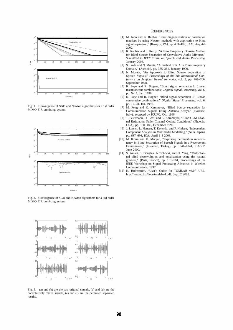
To test the performance of the algorithm on realspeech data two independent segments of speech wereused as input signals to the MIMO FIR mixing sys-tem given in Equation (20). These signals were both4 seconds long and sampled at 8kHz. The signalswere convolutively mixed with the synthetic mixingsystem to obtain 2 mixed signals. With the assump-tion that speech is quasi-stationary over a period ofapproximately 20ms, the observed mixed signals werebuffered and segmented into 401 frames each having160 samples in length. The non-stationarity assumptionassumes that the SOS in each frame does not change.The correlation matricesRτ

XX ,k can be found viaEquations (15,16) forK = 401 frames of the twomixed signals. This allows the method of joint diago-nalization by minimizing the off-diagonal elements ofthe correlation matrices of the recovered signals at eachrespective time lagτ as defined in Equations (17,19).Figure 3 shows the input, mixed and recovered speechsignals. A good qualitative recovery is confirmed bysubjective listening to the recovered audio signals andinspection of graphs (e) and (f) in Figure 3.

VI. CONCLUSION

A new method for convolutive BSS in the timedomain using an existing instantaneous BSS frame-work has been presented. This method avoids theinherent permutation problem when dealing with solv-ing the convolutive BSS problem in the frequencydomain. Optimization algorithms including SGD andNewton methods have been compared for convolutivemixing environments. Future work will be directedat implementing the simulations with recorded datasuch as speech in real reverberant environments wherethe orders of the mixing and un-mixing MIMO FIRsystems are very high.

0 20

20

40

40

60

60

80

80

100

100

120

120

140

140

160

160

180

180

10−40

10−30

10−20

10−10

100

Gradient Method

J(W

)

Iteration k

010

−40

10−30

10−20

10−10

100

Newton Method

Fig. 1. Convergence of SGD and Newton algorithms for a 1st orderMIMO FIR unmixing system.

0 20 40 60 80 100 120 140 160 18010

−20

10−15

10−10

10−5

100

Iteration k

J(W

)

Gradient Method

0 20 40 60 80 100 120 140 160 18010

−20

10−15

10−10

10−5

100

Newton Method

Fig. 2. Convergence of SGD and Newton algorithms for a 3rd orderMIMO FIR unmixing system.

0 1 2 3x 10

x 10

x 10

x 10

x 10

x 10

4

4

4 4

4

4

−0.5

0

0.5

0 1 2 3−0.5

0

0.5

0 1 2 3−1

−0.5

0

0.5

1

0 1 2 3−1

−0.5

0

0.5

1

0 1 2 3−0.5

0

0.5

0 1 2 3−0.5

0

0.5

(a) (b)

(c) (d)

(e) (f)

Fig. 3. (a) and (b) are the two original signals, (c) and (d) are theconvolutively mixed signals, (e) and (f) are the permuted separatedresults.

REFERENCES

[1] M. Joho and K. Rahbar, “Joint diagonalization of correlationmatrices by using Newton methods with application to blindsignal separation,” (Rossyln, VA), pp. 403–407, SAM, Aug 4-62002.

[2] K. Rahbar and J. Reilly, “A New Frequency Domain Methodfor Blind Source Separation of Convolutive Audio Mixtures,”Submitted to IEEE Trans. on Speech and Audio Processing,January 2003.

[3] S. Ikeda and N. Murata, “A method of ICA in Time-FrequencyDomain,” (Aussois), pp. 365–361, January 1999.

[4] N. Murata, “An Approach to Blind Source Separation ofSpeech Signals,”Proceedings of the 8th International Con-ference on Artificial Neural Networks, vol. 2, pp. 761–766,September 1998.

[5] K. Pope and R. Bogner, “Blind signal separation I: Linear,instantaneous combinations,”Digitial Signal Processing, vol. 6,pp. 5–16, Jan. 1996.

[6] K. Pope and R. Bogner, “Blind signal separation II: Linear,convolutive combinations,”Digitial Signal Processing, vol. 6,pp. 17–28, Jan. 1996.

[7] M. Feng and K. Kammeyer, “Blind Source separation forCommunication Signals Using Antenna Arrays,” (Florence,Italy), accepted by ICUPC, Oct. 1998.

[8] T. Petermann, D. Boss, and K. Kammeyer, “Blind GSM Chan-nel Estimation Under Channel Coding Conditions,” (Phoenix,USA), pp. 180–185, December 1999.

[9] J. Larsen, L. Hansen, T. Kolenda, and F. Nielsen, “IndependentComponent Analysis in Multimedia Modelling,” (Nara, Japan),pp. 687–696, ICA, April 1-4 2003.

[10] M. Ikram and D. Morgan, “Exploring permutation inconsis-tency in Blind Separation of Speech Signals in a ReverberantEnvironment,” (Instanbul, Turkey), pp. 1041–1044, ICASSP,June 2000.

[11] S. Amari, S. Douglas, A.Cichocki, and H. Yang, “Multichan-nel blind deconvolution and equalization using the naturalgradient,” (Paris, France), pp. 101–104, Proceedings of theIEEE Workshop on Signal Processing Advances in WirelessCommunications, 1997.

[12] K. Holmstrom, “User’s Guide for TOMLAB v4.0.” URL:http://tomlab.biz/docs/tomlabv4.pdf, Sept. 2 2002.