Embed Size (px)
Citation preview

ARTICLE IN PRESS
0925-2312/$ - se
doi:10.1016/j.ne
�CorrespondE-mail addr
Neurocomputing 69 (2006) 1442–1457
www.elsevier.com/locate/neucom
Optimizing blind source separation with guided genetic algorithms
J.M. Gorriza, C.G. Puntonetb, F. Rojasb, R. Martinc, S. Hornilloc, E.W. Langd,�
aDepartment Signal Theory and Communications, Facultad de Ciencias, University of Granada, Fuentenueva s/n 18071, Granada, SpainbDepartment Architecture and Computer Technology, E.T.S.I. Informatica, University of Granada, Daniel Saucedo s/n 18071, Granada, Spain
cDepartment of Signal Theory and Communications, Escuela Superior de Ingenieros, University of Seville, Camino de los Descubrimientos 41092,
Sevilla, SpaindInstitute of Biophysics, University of Regensburg, UniversitatsstraX e 31 D-93040 Regensburg, Germany
Available online 10 February 2006
Abstract
This paper proposes a novel method for blindly separating unobservable independent component (IC) signals based on the use of a
genetic algorithm. It is intended for its application to the problem of blind source separation (BSS) on post-nonlinear mixtures. The
paper also includes a formal proof on the convergence of the proposed algorithm using guiding operators, a new concept in the GA
scenario. This approach is very useful in many fields such as forecasting indexes in financial stock markets, where the search for
independent components is the major task to include exogenous information into the learning machine; or biomedical applications which
usually use a high number of input signals. The guiding GA (GGA) presented in this work, is able to extract IC with faster rate than the
previous ICA algorithms, as input space dimension increases. It shows significant accuracy and robustness than the previous approaches
in any case. In addition, we present a simple though effective contrast function which evaluates individuals of each population (candidate
solutions) based (a) on estimating the probability densities of the outputs through histogram approximation and (b) evaluating higher-
order statistics of the outputs.
r 2006 Elsevier B.V. All rights reserved.
Keywords: Independent component analysis (ICA); Genetic algorithm (GA); Guiding genetic algorithm (GGA); Higher order statistics (HOS); Mutual
information
1. Introduction
The guiding principle for independent componentanalysis (ICA) is statistical independence, meaning thatthe value of any of the components gives no informationon the values of the other components. This method differsfrom other statistical approaches such as principalcomponent analysis (PCA) and factor analysis preciselyin the fact that it is not a correlation-based transformation,but also reduces higher-order statistical dependencies. Thestarting point in ICA research can be found in [2] where aprinciple of redundancy reduction as a coding strategy inneurons was suggested, i.e. each neural unit was supposedto encode statistically independent features over a set ofinputs. But it was in the 1990s when Bell and Sejnowskiapplied this theoretical concept to blindly separate mixed
e front matter r 2006 Elsevier B.V. All rights reserved.
ucom.2005.12.030
ing author.
ess: [email protected] (E.W. Lang).
sources using a well-known stochastic gradient learningrule [3], thus initiating a productive period of research inthis area [5,7,15,20]. In this way ICA algorithms have beenapplied successfully to several fields such as biomedicine,speech, sonar and radar, signal processing, etc. and morerecently also to time series forecasting using stock data [11].In the latter application, the mixing process of multiplesensors is based on linear transformations making thefollowing assumptions:
(1)
the original (unobservable) sources are statisticallyindependent which are related to social-economicevents;(2)
the number of sensors (stock series) is equal to that ofsources;(3)
the Darmois–Skitovich conditions are satisfied [4].The extensive use of ICA as the statistical technique forsolving blind source separation (BSS) may have led in some

ARTICLE IN PRESS
Fig. 1. Schematic representation of the separation system in ICA-GA.
J.M. Gorriz et al. / Neurocomputing 69 (2006) 1442–1457 1443
situations to the erroneous utilization of both concepts asequivalent. In any case, ICA is just the technique which incertain situations can be sufficient to solve a given problem,that of BSS. In fact, statistical independence insuresseparation of sources in linear mixtures, up to the knownindeterminacies of scale and permutation. However,generalizing to the situation in which mixtures are theresult of an unknown transformation (linear or not) of thesources, independence alone is not a sufficient condition inorder to accomplish BSS successfully. Indeed, in [16] it isformally demonstrated how for nonlinear mixtures, aninfinity of mutually independent solutions can be foundthat have nothing to do with the unknown sources. Thus,in order to successfully separate the observed signals into awave-preserving estimation of the sources, we needadditional information about either the sources or themixing process.
On the other hand, there is a wide class of interestingapplications for which no reasonably fast algorithms havebeen developed, i.e. optimization problems that appearfrequently in several applications such as VLSI design orthe travelling salesman problem. In general, any abstracttask to be accomplished can be viewed as a search througha space of potential solutions and whenever we work withlarge spaces, GAs are suitable artificial intelligencetechniques for developing this optimization [18]. GA arestochastic algorithms whose search methods model somenatural phenomena according to genetic inheritance andDarwinian strife for survival. Such search requires balan-cing two goals: exploiting the best solutions and exploringthe whole search space. In order to carry out them out, GAperforms an efficient multi-directional search maintaining apopulation of potential solutions instead of methods suchas simulated annealing or Hill Climbing.
In this work we apply GA to ICA in the search of theseparation matrix, in order to improve speeding upconvergence rates of the real-time series applications (i.e.EEG and scenarios with the BSS problem in higherdimension) and proving the convergence to the optimum.
2. Definition of ICA
We define ICA using a statistical latent variables model(Jutten and Herault, 1991). Assuming the number ofsources n is equal to the number of mixtures, the linearmodel can be expressed as follows:
xjðtÞ ¼ bj1s1 þ bj2s2 þ � � � þ bjnsn 8j ¼ 1; . . . ; n, (1)
where we explicitly emphasize the time dependence of thesamples of the random variables and assume that both themixture variables and the original sources have zero meanwithout loss of generality. Using matrix notation instead ofsums and including additive noise, the latter mixing modelcan be written as follows:
xðtÞ ¼ B � sðtÞ þ bðtÞ, (2)
or
sðtÞ ¼ A � xðtÞ þ cðtÞ; where A ¼ B�1,
cðtÞ ¼ �B�1 � bðtÞ. ð3Þ
Due to the nature of the mixing model we are able toestimate the original sources ~si and the de-mixing weightsbij applying i.e. ICA algorithms based on higher orderstatistics like cumulants
~si ¼XN
i¼1
bijxj. (4)
Using vector–matrix notation and defining a time seriesvector x ¼ ðx1; . . . ;xnÞ
T, s, ~s and the matrix A ¼ faijg andB ¼ fbijg we can write the overall process as follows:
~s ¼ Bx ¼ BAs ¼ Gs, (5)
where we define G as the overall transfer matrix. Theestimated original sources will be, under some conditionsincluded in the Darmois–Skitovich theorem [4], a permutedand scaled version of the original ones. Thus, in general, itis only possible to find G such that G ¼ PD where P is apermutation matrix and D is a diagonal scaling matrix(Fig. 1).
2.1. Post-non-linear model
The linear assumption is an approximation of nonlinearphenomena in many real world situations. Thus, the linearassumption may lead to incorrect solutions. Hence,researchers in BSS have started addressing the nonlinearmixing models; however, a fundamental difficulty innonlinear ICA is that it is highly non-unique without someextra constraints, therefore, finding independent compo-nents does not lead us necessarily to the originalsources [16].BSS in the nonlinear case is, in general, impossible. Taleb
and Jutten [24] added some extra constraints to thenonlinear mixture so that the nonlinearities are indepen-dently applied in each channel after a linear mixture (seeFig. 2). In this way, the indeterminacies are the same as for

ARTICLE IN PRESS
Fig. 2. Post-nonlinear model.
1In practice, we need independence between sources two against two.
J.M. Gorriz et al. / Neurocomputing 69 (2006) 1442–14571444
the basic linear instantaneous mixing model: invertiblescaling and permutation.
The mixture model can be described by the followingequation:
xðtÞ ¼ FðA � sðtÞÞ. (6)
The unmixing stage, which will be performed by thealgorithm here proposed is expressed by
yðtÞ ¼W �G:ðxðtÞÞ (7)
The post-nonlinearity assumption is reasonable in manysignal processing applications where the nonlinearities areintroduced by sensors and preamplifiers, as usuallyhappens in speech processing. In this case, the nonlinearityis assumed to be introduced by the signal acquisitionsystem.
2.2. Statistical independence criterion based on cumulants
The statistical independence of a set of random variablescan be described in terms of their joint and individualprobability distribution. The independence condition forthe independent components of the output vector y is givenby the definition of independence of random variables:
pyðyÞ ¼Yn
i¼1
pyiðyiÞ, (8)
where py is the joint pdf of random vector (observedsignals) y and pyi
is the marginal pdf of yi. In order tomeasure the independence of the outputs we express Eq. (8)in terms of higher order statistics (cumulants) using thecharacteristic function (or moment generating function)fðkÞ, where k is a vector of variables in the Fouriertransform domain, and considering its natural logarithmF ¼ logðfðkÞÞ. We first evaluate the difference between theterms in Eq. (8) to get
pðyÞ ¼ pyðyÞ �Yn
i¼1
pyðyiÞ
����������2
, (9)
where the norm k . . . k2 can be defined using the convolu-tion operator with different window functions according tothe specific application [25] as follows:
kF ðyÞk2 ¼
ZfF ðyÞ � vðyÞg2 dy (10)
and vðyÞ ¼Qn
i¼1 vðyiÞ. In the Fourier domain and takingnatural log (in order to use higher order statistics, i.e.
cumulants) this equation transforms into:
PðkÞ ¼Z
WyðkÞ �Xn
i¼1
WyiðkiÞ
����������2
VðkÞdk, (11)
where W is the cumulant generating or characteristicfunction (the natural log of the moment generatingfunction) and V is the Fourier transform of the selectedwindow function vðyÞ. If we take Taylor expansion aroundthe origin of the characteristic function we obtain:
WyðkÞ ¼Xl
1
l!qjljWy
qkl11 . . . qkln
n
ð0Þkl11 . . . k
lnn , (12)
where we define jlj � l1 þ � � � þ ln, l � fl1 . . . lng, l! �l1! . . . ln! and:
WyiðkiÞ ¼
Xli
1
li!
qliWyi
qklii
ð0Þklii , (13)
where the factors in the latter expansions are the cumulantsof the outputs (cross and not cross cumulants):
Cl1...lny1...yn¼ ð�jÞjlj
ql1þ���þlnWy
qkl11 . . . qkln
n
ð0Þ
Cliyi¼ ð�jÞ
liqliWyi
qklii
ð0Þ. ð14Þ
Thus, if we define the difference of the terms in Eq. (11) asfollows:
bl ¼1
l!ðjÞjlj
Cly
(15)
that contains the infinite set of cumulants of the outputvector y. Substituting (15) into (11) we have
PðkÞ ¼Z X
l
blkl11 . . . k
lnn
����������2
VðkÞdk. (16)
Hence vanishing cross-cumulants are a necessary conditionfor y1; . . . ; yn to be independent.1 Eq. (16) can betransformed into:
PðkÞ ¼Z X
l;l�
blb�
l�kl1þl
�1
1 . . . klnþl�nn VðkÞdk. (17)
Finally, interchanging the sequence of summation andintegral we can rewrite Eq. (17) as follows:
P ¼Xl;l�
blb�
l�Cl;l� , (18)
where C ¼R
kl1þl
�1
1 . . . klnþl�nn VðkÞdk. In this way, we finally
describe the fitness function f in the evolutionary processin terms of Eq. (18). In practice, we must impose someadditional restrictions to f, it will be a version of theprevious one but limiting the set l. That is, we only considera finite set of cumulants fl; l�g such us jlj þ jl�jo~l.Mathematically, we can express this restriction

ARTICLE IN PRESSJ.M. Gorriz et al. / Neurocomputing 69 (2006) 1442–1457 1445
as follows:
P ¼Xfl;l�g
blb�
l�Cl;l� ; jlj þ jl�jo~l. (19)
A similar expression can be found in [25] but in terms ofmoments. The latter defined function satisfies the definitionof a contrast function C defined in [8] as can be seen in thefollowing generalized proposition given in [9].
Proposition 1. The criterion of statistical independence
based on cumulants defines a contrast function C given by
cðGÞ ¼ P� log j detðGÞj � hðsÞ, (20)
where hðsÞ is the entropy of the sources and G is the overall
transfer matrix.
Proof. To prove this proposition see Appendix A in [9] andapply the multi-linear property of the cumulants [6]. &
2.3. Mutual information approximation
The proposed algorithm will be based on the estimationof mutual information value which cancels out when thesignals involved are independent. Mutual information I
between the elements of a multi-dimensional variable y isdefined as follows:
Iðy1; y2; . . . ; ynÞ ¼Xn
i¼1
HðyiÞ �Hðy1; y2; . . . ; ynÞ, (21)
where HðxÞ is the entropy measure of the random variableor variable set x.
For Eq. (21), in the case that all components y1 . . . yn areindependent, the joint entropy is equal to the sum ofthe marginal entropies. Therefore, mutual information willbe zero. In the rest of the cases (not independentcomponents), the sum of marginal entropies will be higherthan the joint entropy, leading thus to a positive value ofmutual information.
In order to exactly compute mutual information, weneed also to calculate entropies, which likewise requireknowing the analytical expression of the probabilitydensity function (PDF) which is generally not available inpractical applications of speech processing. Thus, wepropose to approximate densities through the discretiza-tion of the estimated signals building histograms and thencalculate their joint and marginal entropies. In this way, wedefine a number of bins m that covers the selectedestimation space and then we calculate how many pointsof the signal fall in each of the bins (Bi i ¼ 1; . . . ;m).Finally, we easily approximate marginal entropies using thefollowing formula:
HðyÞ ¼ �Xn
i¼1
pðyiÞ log2 pðyiÞ � �Xm
j¼1
CardðBjðyÞÞ
n
�log2CardðBjðyÞÞ
n, ð22Þ
where CardðBÞ denotes cardinality of set B, n is the numberof points of estimation y, and (Bj) is the set of points whichfall in the ðjthÞ bin.The same method can be applied for computing the joint
entropies of all the estimated signals:
Hðy1; . . . ; ypÞ ¼Xp
i¼1
Hðyijyi�1; . . . ; y1Þ
� �Xm
i1¼1
Xm
i2¼1
� � �Xm
in¼1
CardðBi1 i2...ipðyÞÞ
n
�log2
CardðBi1 i2 ...ipðyÞÞ
n, ð23Þ
where p is the number of components which need to beapproximated and m is the number of bins in eachdimension.Therefore, substituting entropies in Eq. (21) by approx-
imations of Eqs. (22) and (23), we obtain an approximationof mutual information (Eq. (24)) which will reach itsminimum value when the estimations are independent:
EstðIðyÞÞ
¼Xp
i¼1
EstðHðyiÞÞ � EstðHðyÞÞ
¼ �Xp
i¼1
Xm
j¼1
CardðBjðyiÞÞ
nlog2
CardðBjðyiÞÞ
n
" #
þ � � � þXm
i1¼1
Xm
i2¼1
� � �Xm
in¼1
CardðBi1 i2 ���ipðyÞÞ
n
�log2
CardðBi1 i2 ���ipðyÞÞ
n, ð24Þ
where EstðX Þ stands for ‘‘estimation of x’’.Next section describes an evolution-based algorithm that
minimizes the contrast function defined in the previoussub-sections, escaping from local minima.
3. Background of genetic algorithms and Markov chains
A GA can be modelled by means of a time inhomoge-
neous Markov chain (MC) [12] obtaining interestingproperties related with weak and strong ergodicity,convergence and the distribution probability of the process[22]. A canonical GA (CGA) is constituted by operationsof parameter encoding, population initialization, cross-over, mutation, mate selection, population replacement,fitness scaling, etc. proving that with these simple operatorsa GA does not converge to a population containing onlyoptimal members. However, there are GAs that convergeto the optimum, The Elitist GA [23] and those whichintroduce Reduction Operators [10]. We have borrowed thenotation mainly from [22] where the model for GAs is ainhomogeneous Markov chain model on probabilitydistributions ðSÞ over the set of all possible populationsof a fixed finite size.

ARTICLE IN PRESSJ.M. Gorriz et al. / Neurocomputing 69 (2006) 1442–14571446
In this section we introduce the notions of strong andweak ergodicity of MCs. We study how these notions arenecessary for the concept of convergence and stabilitysummarizing the key concepts and definitions. Then wepresent the GA used with the new set of operators whichallow us to prove convergence to the optimum in theconvergence analysis section.
3.1. MC basis
We first state the definition of a MC with values in thegeneral space ðX;BÞ where X is a metric space and B is theBorel s�algebra and then present basic ergodic theoremsfor functional of MCs which help us to prove theconvergence of the proposed algorithms to a probabilitydistribution that assigns non-zero probabilities only tothose populations that contain the optimum, and then to auniform probability distribution containing only theoptimum.
Definition 1. Let ðX;BÞ be a measurable space and letðO;F;PÞ be a probability space. A MC is defined as aparticular discrete-time stochastic process x� ¼ fxn; n ¼0; 1; . . .g on X with the Markov property:
Pðxnþ1 2 Bjx0; . . . ; xnÞ ¼ Pðxnþ1 2 BjxnÞ
8B 2 B; n ¼ 0; 1; . . . ð25Þ
The next two definitions introduce the notions of strongand weak ergodicity of MC. These notions are related tothe concept of ‘‘stability’’ and are the first step in thedemonstration of the convergence to the optimum. Ofcourse, the existence of invariant probability measure isassumed during this article [13].
Definition 2. Let x� be a MC on a LCS metric space X withtransition probability function (t.p.f.) P, and assume that P
has an invariant p.m. m. Then x� is said to be weaklyergodic if 2
Pnðx; :Þ ) m 8x 2 X . (26)
Definition 3. Let x� be a MC on X with t.p.f P, and assumethat P has an invariant p.m. m. The MC is said to be
�
2
Strongly ergodic if
kPnðx; :Þ � mk ! 0 8x 2 X . (27)
�
Uniformly ergodic ifsupx2X
kPnðx; :Þ � mk ! 0 8x 2 X . (28)
The latter general definitions are equivalent to defini-tions in terms of ergodicity coefficients [17] or stationarydistributions [1] or the asymptotic property of the sequenceof probability distributions. They are also related to the
‘‘)’’ denotesR
f dmn !R
f dm.
effect of the initial distribution of states and to theconvergence to a certain probability distribution matrixin time.
3.2. GA basis
Let C be the set of all possible creatures in a given worldand a function f : C! Rþ be called fitness function. LetX : C!VC a bijection from the creature space onto thefree vector space over A‘, where A ¼ faðiÞ; 0pipa� 1gis the alphabet which can be identified by V1 the freevector space over A. Then we can establish VC ¼ �
‘l¼1V1
and define the free vector space over populations VP ¼
�Ns¼1VC with dimension L ¼ ‘ �N and aL elements.
Finally, let S VP be the set of probability distributionsover PN, that is the state which identifies populations withtheir probability value.In the initial population generation step (choosing
randomly p 2}N , where }N is the set of populations, i.e.the set of N-tuples of creatures containing aL�N�‘ elements).3
After the initial population p has been generated, the fitnessof each chromosome ci is determined using a contrastfunction (i.e. based on cumulants or neg-entropy) whichmeasures the pair-wise statistical independence betweensources in the current individual (see Section 2). The nextstep in CGA is to define the selection operator. Newgenerations for mating are selected depending on theirfitness function values using roulette wheel selection. Letp ¼ ðc1; . . . ; cNÞ 2}N , N 2N and f the fitness functionacting in each component of p. Scaled fitness selection of p
is a lottery for every position 1pipN in population p suchthat creature cj is selected with probability proportional toits fitness value. Thus, proportional fitness selection can bedescribed by column stochastic matrices Fn, N 2N, withcomponents:
hq;Fnpi ¼YaL�1
i¼0
ziqf nðp; qiÞPN
j¼1 f nðp; jÞ, (29)
where p; q 2}N so pi; qi 2 C, h. . .i denotes the standardinner product, and ziq the number of occurrences of qi in p.Once the two individuals have been selected, an elementarycrossover operator CðK ;PcÞ is applied (setting the crossoverrate at a value, i.e. Pc ! 0, which implies children similar toparent individuals) that is given (assuming N even) by
CðK ;PcÞ ¼YN=2i¼1
ðð1� PcÞIþ PcCð2i � 1; 2i; kiÞÞ, (30)
where Cð2i � 1; 2i; kiÞ denotes elementary crossover opera-tion of ci; cj creatures at position 1pkp‘ and I the identitymatrix, to generate two offspring (see [22] for furtherproperties of the crossover operator), K ¼ ðk1; . . . ; kN=2Þ avector of cross over points and Pc the cross overprobability. The next step in a CGA is the mutation
3In our application we assume that creatures lie in a bounded region
½�1; 1, i.e. components of the mixing matrix.

ARTICLE IN PRESSJ.M. Gorriz et al. / Neurocomputing 69 (2006) 1442–1457 1447
operator. The mutation operator used in the algorithm is anextension of the standard one.
3.3. Local search multiple-spot mutation
Let m 2 f0; a� 1=ag. Local search multiple spot mutationis defined as the following procedure:
�
4
exp
For l ¼ 1; . . . ;L do the following steps.
� Decide whether or not mutation takes place at spot l inthe current population with probability
PmðiÞ ¼ m � exp�modfði � 1Þ=Ng
;
� �,
where ; is a normalization constant and m the changeprobability at the beginning of each creature pi inpopulation p.4
�
If mutation takes places at spot l, then change the currentletter in the underlying alphabet A in accordance with thebasic mutation matrix m1. The following propositioncollects the spectral information about the stochasticmatrixMm;; describing local search multiple-spot mutation.
Proposition 2. Let Mm;; denote the symmetric, stochastic
matrix acting on V} describing transition probabilities for
entire populations under local search multiple-spot mutation.
We have
(1)
A
o
Let p; q 2}N . The coefficients of Mm;; are as follows:
hq;Mm;;pi ¼m
a� 1
� �Dðp;qÞ
� exp �XDðp;qÞdif ðiÞ
modfði � 1Þ=Ng
;
!
�YL�Dðp;qÞ
equðiÞ
½1� PmðiÞ, ð31Þ
where Dðp; qÞ is the Hamming distance between p and q
2}N , dif ðiÞ resp. equðiÞ is the set of indexes where p and
q are different resp. equal.
(2) Checking how the matrices act on populations:Mm;; ¼YNl¼1
ð½1� PmðiÞ1þ PmðiÞm1ðlÞÞ, (32)
where m1ðlÞ ¼ 1� 1 � � � � m
1z}|{l
� � � � � 1 is a linear
operator on V}, the free vector space over AL and m
1
is the linear 1-bit mutation operator on V 1, the free
vector space over A. The latter operator is defined acting
on Alphabet as follows:
haðt0Þ; m1aðtÞi ¼ ða� 1Þ�1; 0pt0atpa� 1 (33)
i.e. probability of change a letter in the Alphabet once
mutation occurs with probability equal to Lm.
multi-bit mutation operator with changing probability following an
nential law with respect to the position 1pipL in p 2}N .
(3)
The spectrum can be evaluated according to the followingexpression:
spðMm;;Þ ¼ 1�mðlÞ
a� 1
� �l
; l 2 ½0;L
( ), (34)
where
mðlÞ ¼ am � exp�modfðl� 1ÞNg
;
� �.
Consequently, Mm;; is fully C� positive (since
hq;Mm;;pi40) and is invertible (eigenvalues a0), except
for mðlÞ ¼ ða� 1Þ (then Mm;; ¼ Pe, where Pe is the
orthogonal projection onto the subspace generated by e,the vector of maximal entropy probability distribution).
(4)
Mm;; has similar properties to the constant multiple-bitmutation operator (for ; ! 1), i.e. is a contracting map
in the sense presented in [22]. We can also compare the
coefficients of ergodicity:
trðMm;;ÞptrðMmÞ (35)
where
trðXÞ ¼ maxfkXvkr : v 2 Rn; v ? e and kvkr ¼ 1g.
Mutation is more likely at the beginning of the string ofbinary digits (‘‘small neighborhood philosophy’’).
Definition 4. Let S VP, n; k 2N and fPc;Pmg a varia-tion schedule. A GA is a product of stochastic matrices(mutation, selection, crossover, etc.) acting by matrixmultiplication from the left:
Gn¼ Fn � C
k
Pnc�MPnm
, (36)
where Fn is the selection operator, Ck
Pnc¼ CðK ;PcÞ is the
simple crossover operator and MPnmis the local or standard
mutation operator (see Section 3.3).
In order to improve the convergence speed of thealgorithm we could include another mechanism such aselitist strategy (a further discussion about reductionoperators, can be found in [21]). Another possibility is:
4. Guided genetic algorithms
In order to include statistical information into thealgorithm (it would be a nonsense to ignore it!) we definethe hybrid statistical genetic operator based on reductionoperators as follows (in standard notation acting onpopulations). The value of the probability to go fromindividual pi to qi depends on contrast functions (i.e. basedon cumulants) as follows:
Pðxnþ1 ¼ qijxn ¼ piÞ ¼1
@ðTnÞexp �
jjqi � Sn� pijj
2
Tn
� �,
pi; qi 2 C, ð37Þ
ARTICLE IN PRESS
Table 1
Pseudo-code of GA
Initialize Population
i=0
while not stop do
do N/2 times
Select two mates from piGenerate two offspring using crossover operator
Local Mutate the two children
Include children in new generation pnewend do
Build population pnewApply Guiding Operator (Selection-Elitist Strategies)
to get piþ1i=i+1
end
J.M. Gorriz et al. / Neurocomputing 69 (2006) 1442–14571448
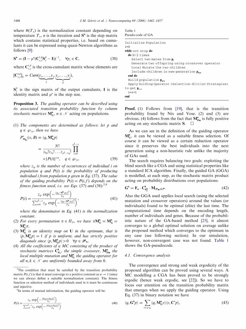
where @ðTnÞ is the normalization constant depending ontemperature Tn, n is the iteration and S
n is the step matrixwhich contains statistical properties, i.e. based on cumu-lants it can be expressed using quasi-Newton algorithms asfollows [9]:
Sn¼ ðI� mnðC
1;by;yS
by � IÞÞ
�1; 8pi 2 C, (38)
where C1;by;y is the cross-cumulant matrix whose elements are
½Ca;by;y ij ¼ Cumðyi; . . . ; yi|fflfflfflfflffl{zfflfflfflfflffl}
a
; yj; . . . ; yj|fflfflfflfflffl{zfflfflfflfflffl}b
Þ,
Sby is the sign matrix of the output cumulants, I is the
identity matrix and mn is the step size.
Proposition 3. The guiding operator can be described using
its associated transition probability function by column
stochastic matrices Mn
G, n 2N acting on populations.
(1)
5T
matr
we
func
and6I
PðiÞ
The components are determined as follows: let p and
q 2}N , then we have
Pn
MGðx;BÞ � hq;Mn
Gpi
¼N!
z0q!z1q! . . . zaL�1q!
YaL�1
i¼0
�fPðiÞgziq; q 2}N , ð39Þ
where ziq is the number of occurrences of individual i on
population q and PðiÞ is the probability of producing
individual i from population p given in Eq. (37). The value
of the guiding probability PðiÞ ¼ Pði; f Þ depends on the
fitness function used, i.e. see Eqs. (37) and (38):5;6
PðiÞ ¼zip exp �
kqi�Sn �pik
2
Tn
� �PaL�1
i¼0 zip exp �kqi�S
n�pi jj2
Tn
� � , (41)
where the denominator in Eq. (41) is the normalization
constant.
(2) For every permutation p 2 PN , we have pMnG¼Mn
G¼
Mn
Gp.
(3)
MnGis an identity map on U in the optimum, that is
hp;Mn
Gpi ¼ 1 if p is uniform; and has strictly positive
diagonals since hp;Mn
Gpi40 8p 2PN.
(4)
All the coefficients of a MC consisting of the product ofstochastic matrices Ck
Pc, the simple crossover, Mn
Pmthe
local multiple mutation and Mn
Gthe guiding operator for
all n; k 2N are uniformly bounded away from 0.
he condition that must be satisfied by the transition probability
ix Pði; f Þ is that it must converge to a positive constant as n! 1 (since
can always define a suitable normalization constant). The fitness
tion or selection method of individuals used in it must be continuous
injective.
n terms of mutual information, the guiding operator will be:
¼zip exp �
jjIðqi ÞþI ðpi Þjj2
Tn
� �PaL�1
i¼0 zip exp �jjI ðqi ÞþIðpi Þjj
2
Tn
� � (40)
Proof. (1) Follows from [19], that is the transitionprobability found by Nix and Vose. (2) and (3) areobvious. (4) follows from the fact that Mn
Pmis fully positive
acting on any stochastic matrix S. &
As we can see in the definition of the guiding operatorMn
G, it can be viewed as a suitable fitness selection. Of
course it can be viewed as a certain reduction operatorsince it preserves the best individuals into the nextgeneration using a non-heuristic rule unlike the majorityof GAs used.The search requires balancing two goals: exploiting the
blind search like a CGA and using statistical properties likea standard ICA algorithm. Finally, the guided GA (GGA)is modelled, at each step, as the stochastic matrix productacting on probability distributions over populations:
Gn¼ Fn � C
k
Pnc�MðPm ;GÞn . (42)
Also the GGA used applies local search (using the selectedmutation and crossover operators) around the values (orindividuals) found to be optimal (elite) the last time. Thecomputational time depends on the encoding length,number of individuals and genes. Because of the probabil-istic nature of the GA-based method [25], it almostconverges to a global optimal solution on average unlikethe proposed method which converges to the optimum inany case (see following section). In our simulation,however, non-convergent case was not found. Table 1shows the GA-pseudocode.
4.1. Convergence analysis
The convergence and strong and weak ergodicity of theproposed algorithm can be proved using several ways. AMC modelling a CGA has been proved to be stronglyergodic (hence weak ergodic, see [22]). So we have tofocus our attention on the transition probability matrixthat emerges when we apply the guiding operator. UsingEq. (37) in binary notation we have
hq;Gnpi ¼X
v2}N
hq;Mn
Gvihv;Cnpi, (43)

ARTICLE IN PRESS
7A scaling sequence fn : ðRþÞ
N! ðRþÞN is a sequence of functions
connected with a injective fitness criterion f as f nðpÞ ¼ fnðf ðpÞÞ p 2}N
such as M1
G¼ limn!1Mn
Gexist.
J.M. Gorriz et al. / Neurocomputing 69 (2006) 1442–1457 1449
where Cn is the stochastic matrix associated to the CGA
and Mn
Gis given by Eq. (39).
Based on the definitions of strong and weak ergodicitywe can establish the following
Proposition 4 (Weak ergodicity). A MC modelling a GGA
satisfies weak ergodicity if the t.p.f associated to guiding
operators converges to uniform populations (populations with
the same individual).
Proof. If we define a GGA on CGAs, the ergodicityproperties depend on the newly defined operator since theysatisfy them as we said before. To prove this propositionwe just have to check the convergence of the t.p.f. of theguiding operator on uniform populations. If the followingcondition is satisfied:
Pn
Gðx;BÞ ! PU; hu;G
npi ! 1 u 2 U. (44)
Then we can find a series of numbers which satisfies:X1n¼1
minn;pðhu;GnpiÞ ¼ 1p
X1n¼1
minq;p
Xv2}N
�minðhv;Mn
Gpihv;CnqiÞ ð45Þ
which is equivalent to weak ergodicity [17]. &
Applying this proposition (a novel necessary conditionof weak ergodicity) to the set of operators used in theexperimental sections we have the following lemma:
Lemma 1. The GA modelled by the time inhomogeneous MC
described in Eq. (41) is weakly ergodic.
Proof. To get this result we have to check Eq. (44) with theproposed operator. If we take limit in the latter expressionwe have that the probability of going from any populationto uniform populations as n tends to infinity is
limn!1hu;Gnpi ! 1 u 2 U (46)
since
hu;Gnpi
¼X
v2}N
N!
z0u!z1u! . . . zaL�1u!|fflfflfflfflfflfflfflfflfflfflfflffl{zfflfflfflfflfflfflfflfflfflfflfflffl}1
�YaL�1
i¼0
zip exp �jjui�S
n �pik2
Tn
� �PaL�1
i¼0 zip exp �kui�S
n �pik2
Tn
� �8<:
9=;ziu
|fflfflfflfflfflfflfflfflfflfflfflfflfflfflfflfflfflfflfflfflfflfflfflfflfflfflfflffl{zfflfflfflfflfflfflfflfflfflfflfflfflfflfflfflfflfflfflfflfflfflfflfflfflfflfflfflffl}n!1 f�g!1
hv;Cnpi
ð47Þ
and Cn is a column stochastic matrix (the sum of its
columns is equal to 1). Hence using Proposition 4 thelemma is proved. &
The strong ergodicity of the MC will be proved using theresults obtained with CGAs in the next proposition:
Proposition 5 (Strong ergodicity). Let Mn
Pmdescribe multi-
ple local mutation, Ck
Pncdescribe a model for crossover and Fn
describe the fitness selection. Let ðPn
m;Pn
cÞn 2N be a
variation schedule and ðfnÞn2N a fitness scaling sequence
associated to Mn
Gdescribing the guiding operator according
to this scaling.7 Let Cn¼ F
n�M
n
Pm� C
k
Pncrepresent the first n
steps of a CGA. In this situation,
v1 ¼ limn!1
Gnv0 ¼ lim
n!1ðM1
GC1Þ
nv0 (48)
exists and is independent of the choice of v0, the initial
probability distribution. Furthermore, the coefficients hv1; piof the limit probability distribution are strictly positive for
every population p 2}N .
Proof. The demonstration of this proposition is ratherobvious using the results of Theorem 16 in [22] and point 4in Proposition 3. In order to obtain the results of the lattertheorem we only have to replace the canonical selectionoperator Fn with our guiding selection operator Mn
Gwhich
has the same essential properties. &
At this moment, we only have demonstrated that ouralgorithm behaves the same as CGAs. Now we have toprove the convergence to optimal populations. Of course, itis necessary that the MC modelling the GGA must bestrongly ergodic. The following result shows that thesequence of stochastic matrices modelling the GGAconverges to a probability distribution that assigns non-zero probabilities only to those uniform populations thatcontain the optimum (all the individuals being the same).
Proposition 6 (Convergence to the optimum). Let Mn
Pm
describe multiple local mutation, Ck
Pncdescribe a model for
crossover and Fn describe the fitness selection. Let
ðPn
m;Pn
cÞn 2N be a variation schedule and ðfnÞn2N a fitness
scaling sequence associated to Mn
Gdescribing the guiding
operator according to this scaling and given in Lemma 1. Let
Cn¼ F
n�M
n
Pm� C
k
Pncrepresent the first n steps of a CGA. In
this situation, the GGA algorithm converges to the optimum.
Proof. To reach this result, one has to prove that theprobability to go from any uniform population to thepopulation p� containing only the optimum is equal to 1when n!1:
limn!1hp�;Gnui ¼ 1 (49)
since the GGA is an strongly ergodic MC hence anypopulation tends to uniformity in time. If we check thisexpression (similar to (47)) we finally have Eq. (49). Thus,any guiding operator following a simulated annealing lawconverges to the optimum uniform population in time. &
Assembling all the properties and restrictions describedalong the paper we can finally reach to the followingproposition:

ARTICLE IN PRESS
g1 = 3x 5 + 2x 3 + 4.25x,
g2 = 2.14x 5 + 12x.
3 2 4.25 2.14 0 12
Chromosome
Gene
Fig. 3. Encoding example for p ¼ 2 signals and polynomials up to grade 5.
1. Randomly initialize population
2. Create offspring throughgenetic operators
3. Evaluate the fitness ofeach candidate solution
(independence of outputs y)
4. Apply elitist selection
6. Solution y = g [W.x]
5. Termiante?(nr. Iteration = max)
(taking g from best solution and W from FastICA)
Yes
No
Fig. 4. Genetic algorithm scheme for post-nonlinear blind separation of
sources.
J.M. Gorriz et al. / Neurocomputing 69 (2006) 1442–14571450
Proposition 7. Any contrast function C can be used to build
a transition matrix probability PðiÞ in the guiding operator
Mn
Gsatisfying Proposition 6.
Proof. It is obvious that a contrast function can be used asfitness function. By definition a contrast function is nullonly in the separation point. A selection based on acontrast function does not ignore spatial structure withinthe population unlike standard selection. The injectiveproperty ofC can be achieved independently of it replacingits fitness value of each creature by eCðpiÞ ¼ CðpiÞþ
kpik2 pi 2 C. Applying the norm and a normalizationconstant into the new function we get a fully positive andstochastic guiding matrix. The guiding operator is definedfor any contrast function as follows:
hq;Mn
Gpi ¼
Xv2}N
N!
z0q!z1q! . . . zaL�1q!
YaL�1
i¼0
�zip � P kCðqiÞk
2� �PaL�1
i¼0 zip � P kCðqiÞk2
� �( )ziq
, ð50Þ
where P is a decreasing p.d.f. (definite positive) andsatisfying that it tends to a constant (greater than zero)in time. &
5. Experimental framework
This section illustrates the validity of the geneticalgorithms here proposed and investigates the accuracyof the method. We combined voice signals and noisenonlinearly and then try to recover the original sources. Inorder to measure the accuracy of the algorithm, weevaluate it using the mean square error (MSE) and thecrosstalk in decibels (CT):
MSEi ¼
PN
t¼1 ðsiðtÞ � yiðtÞÞ2
N,
CTi ¼ 10 log
PN
t¼1 ðsiðtÞ � yiðtÞÞ2PN
t¼1 ðsiðtÞÞ2
!. ð51Þ
5.1. Non-linear ICA examples
First of all, it should be recalled that the proposedalgorithm needs to estimate two different mixtures (seeEq. (2)): a family of nonlinearities g which approximatesthe inverse of the nonlinear mixtures f and a linearunmixing matrix W which approximates the inverse ofthe linear mixture A. This linear demixing stage will beperformed by the well-known FastICA algorithm byHyvarinen and Oja [14]. To be precise, FastICA will beembedded into the GA in order to approximate the linearmixture.
Therefore, the encoding scheme for the chromosome inthe post-nonlinear mixture will be the coefficients of theodd polynomials which approximate the family of non-
linearities g. Fig. 3 shows an example of polynomialapproximation and encoding of the inverse non-linearities.The fitness function is easily derived from Eq. (24) which
is precisely the inverse of the approximation of mutualinformation, so that the GA maximizes the fitness function,which is more usual in evolution programs literature
FitnessðyÞ ¼1
EstðIðyÞÞ. (52)
Expression (52) obeys to the desired properties of acontrast function [8], that is, a mapping c from the set ofprobability densities fpx; x 2 RN
g to R satisfying the fol-lowing requirements:
(1)
cðpxÞ does not change if the components of ðxiÞ arepermuted.(2)
cðpxÞ is invariant to invertible scaling. (3) If x has independent components, then cðpAxÞpcðpxÞ;8A invertible.Regarding other aspects of the GA, the population (i.e.set of chromosomes) was initialized randomly within aknown interval of search for the polynomial coefficients.The genetic operators involved were simple ‘‘One-pointCross-over’’ and ‘‘Non-Uniform Mutation’’ [18]. Selectionstrategy is elitist, keeping the best individual of ageneration for the next one (Fig. 4).

ARTICLE IN PRESS
Sources s Mixtures x Estimations y1
0.5
-0.5
-10 6750 13500
0 6750 13500 0 6750 13500
0 6750 13500 6750 13500
6750 13500
0
1
0.50.5
0
5
-5
0
-0.5-0.5
-1
-1 0 1 -1 0 1
0
1
0.5
-0.5
-1
0
1
0.5
-0.5
-1-10 0 10
0
5
-5
-10
0
1
0.5
-0.5
-1
0
5
-5
0
Fig. 5. Sources, mixtures and estimations (along time and scatter plots in
the bottom line) for two voice signals.
Fig. 6. Original images (s), PNL-mixtures (x) and estimations (y) applying
the genetic algorithm.
J.M. Gorriz et al. / Neurocomputing 69 (2006) 1442–1457 1451
5.1.1. Two voice signals
This experiment corresponds to a ‘‘Cocktail Party Problem’’situation, that is, separating one voice from another. Two voicesignals corresponding to two persons saying the numbers fromone to 10 in English and Spanish were non-linearly mixedaccording to the following matrix and functions:
A ¼1 0:87
�0:9 0:14
; F ¼ ½f 1ðxÞ ¼ f 2ðxÞ ¼ tanhðxÞ. (53)
Then the GA was applied (population size ¼ 40, number ofiterations ¼ 60). Polynomials of fifth order were used as theapproximators for ðg ¼ f
�1Þ. Performance results and a plot of
the original and estimated signals are briefly depicted in (Fig. 5and Eqs. (54) and (55))
MSEðy1; s1Þ ¼ 0:0012; Crosstalkðy1; s1ÞðdBÞ ¼ �17:32 dB,
(54)
MSEðy2; s2Þ ¼ 0:0009 Crosstalkðy2; s2ÞðdBÞ ¼ �19:33 dB.
(55)
As can be seen, estimations (y) are approximately equivalentto the original sources (s) up to invertible scalings andpermutations. E.g. estimation ðy1Þ is scaled and inverted inrelation to ðs1Þ.
5.1.2. Three image signals
In this experiment, source signals correspond to threeimage signals (‘‘Lena’’, ‘‘Cameraman’’, ‘‘University ofGranada emblem’’). They were mixed according to thePNL scheme (Fig. 2) with the following values:
A ¼
0:9 0:3 0:6
0:6 �0:7 0:1
�0:2 0:9 0:7
264375; f ¼
f 1ðxÞ ¼ tanhðxÞ;
f 2ðxÞ ¼ tanhð0:8 � xÞ;
f 3ðxÞ ¼ tanhð0:5 � xÞ
264375.(56)
In this case, the simulation results draw a slightly worseperformance than the former case, due to the increase ofthe dimensionality from two to three sources:
MSEðy1; s2Þ ¼ 0:0006, Crosstalkðy1; s2Þ (dB) ¼
�16:32 dB, MSEðy2; s1Þ ¼ 0:0010, Crosstalkðy2; s1Þ (dB)¼ �12:12 dB, MSEðy3; s3Þ ¼ 0:0011, Crosstalkðy3; s3Þ (dB)¼ �11:58 dB.
Original images can be clearly distinguished through theestimations, although some remains of the other imagesinterfere. Also note that an inversion in the signal resultsobviously in the negative estimation of the source (e.g. thecameraman) (Fig.6).
5.2. Experiments GGA vs GA
At the first step, we compare the previous canonicalmethod to apply GAs to ICA [25] with the GGA versionfor a reduced input space dimension ðn ¼ 3Þ. The computerused in these simulations was a PC 2GHz, 256MB RAMin the case of a low number of signals and the softwareused is an extension of ICATOOLBOX2.0 in MatLab
code, protected by the Spanish law No. CA-235/04. We testthese two algorithms for a set of independent signalsplotted in Fig. 7(a) using 50 randomly chosen mixingmatrices (50 runs); i.e. using the mixing matrix:
B ¼
1:0000 �0:9500 0:5700
�0:5800 1:0000 0:0900
0:6300 �0:0100 1:0000
8><>:9>=>; (57)

ARTICLE IN PRESS
0 0.5 1 1.5 2 2.5 3 3.5 4 4.5 5 0 0.5 1 1.5 2 2.5 3 3.5 4 4.5 5
0 0.5 1 1.5 2 2.5 3 3.5 4 4.5 5 0 0.5 1 1.5 2 2.5 3 3.5 4 4.5 5
x 104
x 104
x 104
x 104
0 0.5 1 1.5 2 2.5 3 3.5 4 4.5 5
x 104
0 0.5 1 1.5 2 2.5 3 3.5 4 4.5 5
x 104
1
− 0.5
0
0.5
− 1
1
− 0.5
0
0.5
− 1
1
− 0.5
0
0.5
− 1
1
− 0.5
0
0.5
− 1
1
− 0.5
0
0.5
− 1
1
− 0.5
0
0.5
(a) (b)
Fig. 7. Set of independent series used in the comparison GA-GGA and a mixed case: (a) original signals; (b) mixed signals.
− 1 −0.8 −0.6 −0.4 −0.2 0 0.2 0.4 0.6 0.8 10
500
1000
1500
2000
2500
3000Sinus
signal 1 signal 2 signal 30.5 0.4 0.3 0.2 0.1 0 0.1 0.2 0.3 0.40
0.5
1
1.5
2
2.5
3x 10
4 Bacalao1.wav
− 1 − 0.8 − 0.6 − 0.4 − 0.2 0 0.2 0.40
2000
4000
6000
8000
10000
12000
14000
16000
(a) (b) (c)
Fig. 8. Histograms: (a) signal 1; (b) signal 2; (c) signal 3.
J.M. Gorriz et al. / Neurocomputing 69 (2006) 1442–14571452
we get the signals shown in Fig. 7(b). We have chosen twosuper-Gaussian signals and one bimodal signal as shown inFig. 8 for the first attempt ðninps ¼ 3Þ and show how theyare transformed into a set of dependent components usingthe matrix in Eq. (57). The order of the statistics used is thesame in both the methods (cumulants of fourth order)8andthe size of population was 100. In this way we can comparethe search efficiency of both methods. Later we will focusour attention with a third statistical algorithm for ICA, the
8Based on the above discussion, we can define the fitness function
approach for BSS as follows:
f ðp0Þ ¼Xi;j;...
kCumðyi; yj ; . . .zfflfflfflfflffl}|fflfflfflfflffl{stimes
Þk 8i; j; . . . 2 ½1; . . . ; n, (58)
where p0 is the parameter vector (individual) containing the separation
matrix and k . . . k denotes the absolute value.
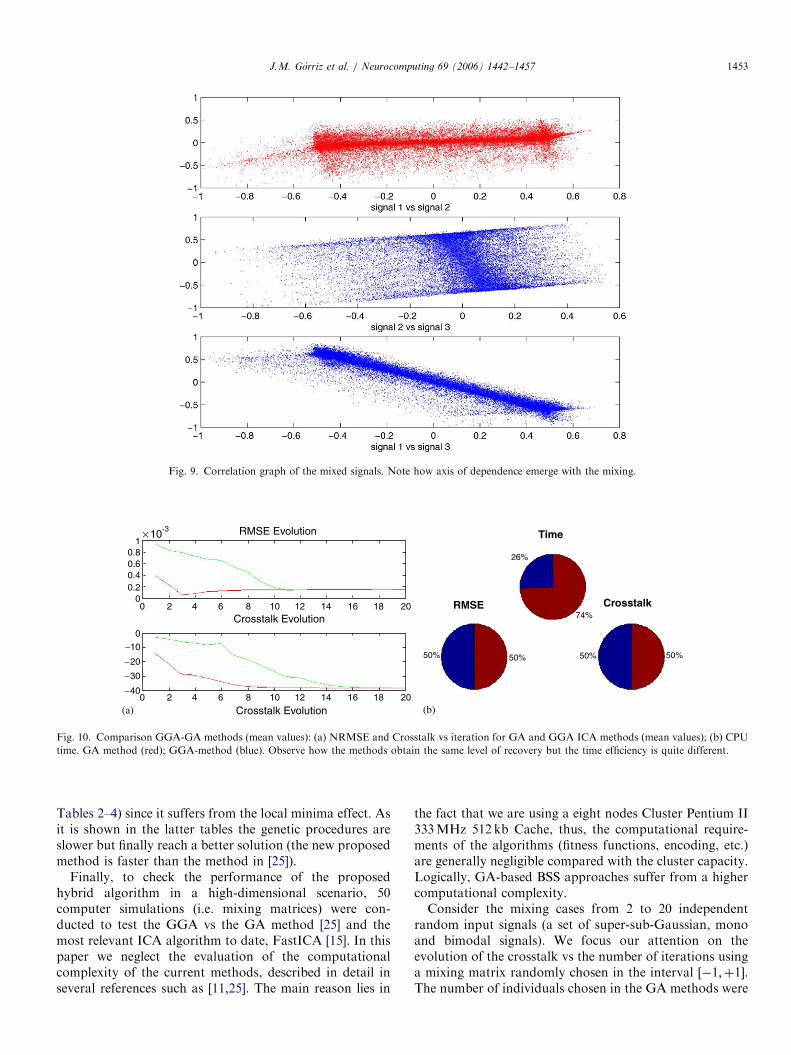
well-known FastICA [15]. This method uses the same levelof information in its contrast function (fourth order) thusthe comparison is significant. Results obtained fromsimulations are conclusive Figs. 9 and 10(a). We see howthe number of iterations needed to reach convergence ishigher using the proposed method in [25]. This is due toblind search strategy used in the latter reference unlike theguided strategy proposed in this paper. We measureconvergence by means of the well-known methods: cross-talk (between original and recovered signals) and normal-ized round mean square error (NRMSE). The set ofrecovering signals using GGA method can be found inFig. 11(b). In the case of the three method comparisonwe observe how the efficiency of the FastICA inlow dimension is better than the genetic approaches (seeFig. 11(a). Somehow the standard deviation in time anderror measure is higher than with the genetic methods (see
ARTICLE IN PRESS
10.80.60.40.2
0
0
0
−10
− 20
− 30
− 40
2 4 6 8 10 12 14 16 18 20Crosstalk Evolution
RMSE Evolution
0 2 4 6 8 10 12 14 16 18 20
Crosstalk Evolution
× 10-3Time
RMSE Crosstalk
26%
74%
50% 50%50% 50%
(a) (b)
Fig. 10. Comparison GGA-GA methods (mean values): (a) NRMSE and Crosstalk vs iteration for GA and GGA ICA methods (mean values); (b) CPU
time. GA method (red); GGA-method (blue). Observe how the methods obtain the same level of recovery but the time efficiency is quite different.
Fig. 9. Correlation graph of the mixed signals. Note how axis of dependence emerge with the mixing.
J.M. Gorriz et al. / Neurocomputing 69 (2006) 1442–1457 1453
Tables 2–4) since it suffers from the local minima effect. Asit is shown in the latter tables the genetic procedures areslower but finally reach a better solution (the new proposedmethod is faster than the method in [25]).
Finally, to check the performance of the proposedhybrid algorithm in a high-dimensional scenario, 50computer simulations (i.e. mixing matrices) were con-ducted to test the GGA vs the GA method [25] and themost relevant ICA algorithm to date, FastICA [15]. In thispaper we neglect the evaluation of the computationalcomplexity of the current methods, described in detail inseveral references such as [11,25]. The main reason lies in
the fact that we are using a eight nodes Cluster Pentium II333MHz 512 kb Cache, thus, the computational require-ments of the algorithms (fitness functions, encoding, etc.)are generally negligible compared with the cluster capacity.Logically, GA-based BSS approaches suffer from a highercomputational complexity.Consider the mixing cases from 2 to 20 independent
random input signals (a set of super-sub-Gaussian, monoand bimodal signals). We focus our attention on theevolution of the crosstalk vs the number of iterations usinga mixing matrix randomly chosen in the interval ½�1;þ1.The number of individuals chosen in the GA methods were

ARTICLE IN PRESS
0 0.5 1 1.5 2 2.5 3 3.5 4 4.5 5
x 104
0 0.5 1 1.5 2 2.5 3 3.5 4 4.5 5
x 104
0 0.5 1 1.5 2 2.5 3 3.5 4 4.5 5
x 104
− 0.5
0
0.5
1
− 0.5
0
1
0.5
1
− 0.5
0
1
0.5
1
(a) (b)31%
31%30%
65%
24%
11%
37%
35%
35%
CrosstalkRMSE
Time
Fig. 11. Set of recovering signals using GGA method and global comparison: (a) set of recovering signals GGA method; (b) comparison for number of
inputs equal to 3 GGA (red), GA (light blue) and FastICA (blue).
Table 2
Mean and deviation of the parameters in the separation over 50 runs for the cost function of fourth order by the GA-method, GGA method and the
FASTICA method
Method Param. a11 a12 a13 a21 a22
GA-ICA mean �0:2562 0.1473 �0:1657 �0:0647 �0:1393dev. (%) p5 p5 p5 p5 p5
GGA-ICA mean �0:1481 0.1647 �0:2564 0.1401 �0:2464dev. (%) p6:5 p6:5 p6:5 p6:5 p6:5
FastICA mean 0.0756 �0:1099 0.2271 �0:0715 0.1648
dev. (%) p10 p10 p10 p10 p10
Table 3
Mean and deviation of the parameters in the separation over 50 runs for the cost function of fourth order by the GA-method, GGA method and the
FASTICA method
Method Param. a23 a31 a32 a33
GA-ICA mean 0.2475 �0:4910 0.0998 �0:0350dev. (%) p5 p5 p5 p5
GGA-ICA mean �0:0649 �0:1003 0.0345 �0:4914dev. (%) p6:5 p6:5 p6:5 p6:5
FastICA mean 0.0659 0.0512 �0:0226 0.4435
dev. (%) p10 p10 p10 p10
Table 4
Mean and deviation of the parameters in the separation over 50 runs for the cost function of fourth order by the GA-method, GGA method and the
FASTICA method (cont)
Method Param. Comp. time (s) NRMSE Crosstalk (dB)
GA-ICA mean 10.21 1:5635�4 �34:709
dev. (%) p2 p1 p1
GGA-ICA mean 3.3 1:5408�4 �37:7507
dev. (%) p2 p1 p1
FastICA mean 1.64 1:6355�4 �29:663
dev. (%) p5 p2 p4
J.M. Gorriz et al. / Neurocomputing 69 (2006) 1442–14571454
ARTICLE IN PRESS
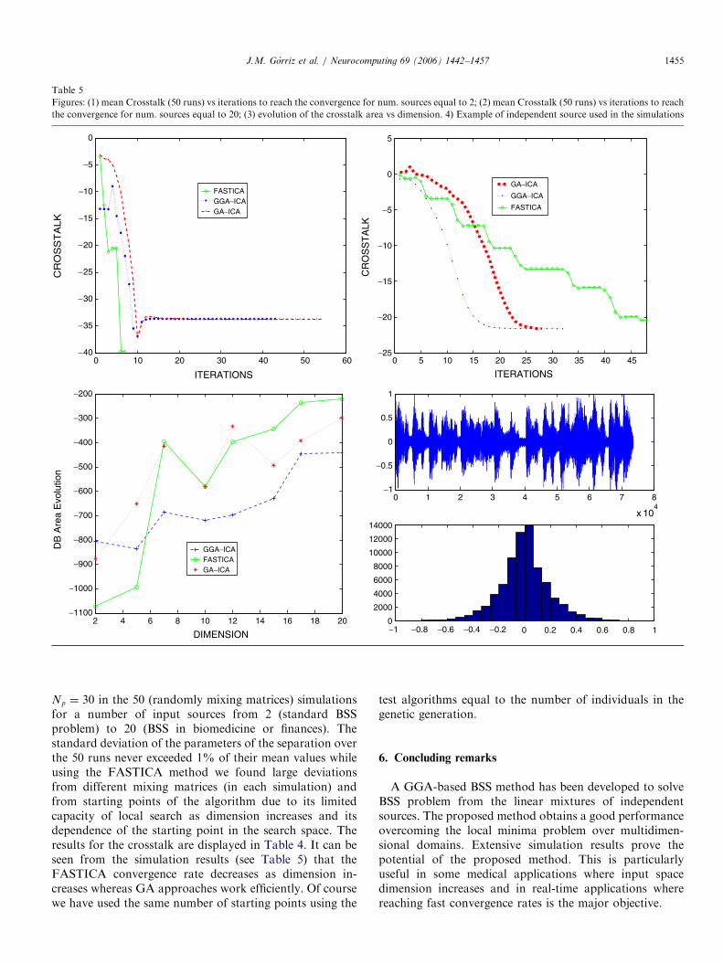
Table 5
Figures: (1) mean Crosstalk (50 runs) vs iterations to reach the convergence for num. sources equal to 2; (2) mean Crosstalk (50 runs) vs iterations to reach
the convergence for num. sources equal to 20; (3) evolution of the crosstalk area vs dimension. 4Þ Example of independent source used in the simulations
0 10 20 30 40 50
5
0
60− 40
− 35
− 30
− 25
− 20
−15
−10
−5
−5
−10
−15
−20
−25
0
ITERATIONS
CR
OS
ST
ALK
0 5 10 15 20 25 30 35 40 45
ITERATIONSC
RO
SS
TA
LK
2 4 6 8 10 12 14 16 18 20−1100
−1000
−900
−800
−700
−600
−500
−400
−300
−200
DIMENSION
DB
Are
a E
volu
tion
GGA−ICAFASTICAGA−ICA
0 1 2 3 4 5 6 7 8
x 104
−1
−0.5
0
0.5
1
−1 −0.8 −0.6 −0.4 −0.2 0 0.2 0.4 0.6 0.8 10
2000
4000
6000
8000
10000
12000
14000
GGA−ICAFASTICA
GA−ICA
GGA−ICA
FASTICA
GA−ICA
J.M. Gorriz et al. / Neurocomputing 69 (2006) 1442–1457 1455
Np ¼ 30 in the 50 (randomly mixing matrices) simulationsfor a number of input sources from 2 (standard BSSproblem) to 20 (BSS in biomedicine or finances). Thestandard deviation of the parameters of the separation overthe 50 runs never exceeded 1% of their mean values whileusing the FASTICA method we found large deviationsfrom different mixing matrices (in each simulation) andfrom starting points of the algorithm due to its limitedcapacity of local search as dimension increases and itsdependence of the starting point in the search space. Theresults for the crosstalk are displayed in Table 4. It can beseen from the simulation results (see Table 5) that theFASTICA convergence rate decreases as dimension in-creases whereas GA approaches work efficiently. Of coursewe have used the same number of starting points using the
test algorithms equal to the number of individuals in thegenetic generation.
6. Concluding remarks
A GGA-based BSS method has been developed to solveBSS problem from the linear mixtures of independentsources. The proposed method obtains a good performanceovercoming the local minima problem over multidimen-sional domains. Extensive simulation results prove thepotential of the proposed method. This is particularlyuseful in some medical applications where input spacedimension increases and in real-time applications wherereaching fast convergence rates is the major objective.
ARTICLE IN PRESSJ.M. Gorriz et al. / Neurocomputing 69 (2006) 1442–14571456
In this work we have focussed our attention to linearmixtures. The nonlinear problem can be interpreted as apiece-wise linear model and is expected that results improveeven more since the higher parameters to encode the betterresults we obtain. GAs are the best strategies in high-dimensional domains so it would be interesting how thesealgorithms (non-CGAs) face the nonlinear ICA. A specificcase of a nonlinear source separation problem has beentackled by an ICA algorithm based on the use of GAs. Asthe separation of sources through the independence basisonly is impossible in nonlinear mixtures, we assumed alinear mixture followed by a nonlinear distortion in eachchannel (Post-Non-Linear model) which constrains thesolution space. Experimental tests showed promisingresults, although future research will focus on the adapta-tion of the algorithm for higher dimensionality andstronger nonlinearities.
In the theoretical section we have proved the convergenceof the proposed algorithm to the optimum unlike the ICAalgorithms which usually suffer from local minima and non-convergent cases. Any injective contrast function can beused to build a guiding operator, as an elitist strategy i.e.the simulated annealing function defined in Section 4.
Acknowledgement
This work has been supported by the SESIBONNTEC2004-06096-C03-00 and the CICYT TIC2001-2845Spanish Projects.
References
[1] S. Anily, A. Federgruen, Ergodicity in parametric nonstationary
Markov chains: an application to simulated annealing methods,
Oper. Res. 35 (6) (1987) 867–874.
[2] H.-B. Barlow, Possible principles underlying transformation of
sensory messages, in: W.A. Rosenblith (Ed.), Sensory Communica-
tion, MIT Press, New York, USA, 1961.
[3] A.-J. Bell, T.-J. Sejnowski, An information-maximization approach
to blind separation and blind deconvolution, Neural Comput. 7
(1995) 1129–1159.
[4] X. Cao, W. Liu, General approach to blind source separation, IEEE
Trans. Signal Process. 44 (3) (1996) 562–571.
[5] J.-F. Cardoso, Infomax and maximun likelihood for source separa-
tion, IEEE Lett. Signal Process. 4 (1997) 112–114.
[6] C. Chryssostomos, A.-P. Petropulu, Higher Order Spectra Analysis:
A Non-linear Signal Processing Framework, 1999.
[7] A. Cichoki, R. Unbehauen, Robust neural networks with on-line
learning for blind identification and blind separation of sources,
IEEE Trans. Circuits Syst. 43 (211) (1996) 894–906.
[8] P. Comon, Independent component analysis, a new concept?, Signal
Process. 36 (1994) 287–314.
[9] S. Cruces, L. Castedo, A. Cichocki, Robust blind source separation
algorithms using cumulants, Neurocomputing 49 (2002) 87–118.
[10] A.-E. Eiben, E.-H. Aarts, K.V. Hee, Global convergence of genetic
algorithms: a Markov chain analysis, Lecture Notes in Computer
Science, vol. 496, Springer, Berlin, pp. 4–12.
[11] J.-M. Gorriz, C.-G. Puntonet, M. Salmeron, J.-G. delaRosa, New
model for time series forecasting using rbfs and exogenous data,
Neural Comput. Appl. J. 13 (2) (2004) 101–111.
[12] O. Haggstrom, Finite Markov Chains and Algorithmic Applications,
1998.
[13] O. Hernandez-Lerma, J.-B. Lasserre, Markov Chains and Invariant
Probabilities, 1995.
[14] A. Hyvarinen, E. Oja, A fast fixed-point algorithm for independent
component analysis, Neural Comput. 9 (7) (1997) 1483–1492.
[15] A. Hyvarinen, E. Oja, A fast fixed point algorithm for independent
component analysis, Neural Comput. 9 (1997) 1483–1492.
[16] A. Hyvarinen, P. Pajunen, Nonlinear independent component
analysis: existence and uniqueness results, Neural Networks 12 (3)
(1999) 429–439.
[17] D.-L. Isaacson, D.-W. Madsen, Markov Chains: Theory and
Applications, 1985.
[18] Z. Michalewicz, Genetic Algorithms þ Data Structures ¼ Evolution
Programs, tercera ed., Springer, New York, 1999.
[19] A.-E. Nix, M.-D. Vose, Modelling genetic algorithms with Markov
chains, Ann. Math. Artif. Intell. 5 (1992) 79–88.
[20] C.-G. Puntonet, A. Prieto, Neural net approach for blind separation
of sources based on geometric properties, Neurocomputing 18 (1998)
141–164.
[21] G. Rudolf, Convergence analysis of canonical genetic algorithms,
IEEE Trans. Neural Networks 5 (1) (1994) 96–101.
[22] L.-M. Schmitt, C.-L. Nehaniv, R.-H. Fujii, Linear analysis of genetic
algorithms, Theoret. Comput. Sci. 200 (1998) 101–134.
[23] J. Suzuki, A Markov chain analysis on simple genetic algorithms,
IEEE Trans. Systems, Man, Cybernetics 25 (4) (1995) 655–659.
[24] A. Taleb, C. Jutten, Source separation in post-nonlinear mixtures,
IEEE Trans. Signal Process. 47 (10) (1999) 2807–2820.
[25] Y. Tan, J. Wang, Nonlinear blind source separation using higher
order statistics and a genetic algorithm, IEEE Trans. Evolutionary
Comput. 5 (6) (2001) 600–612.
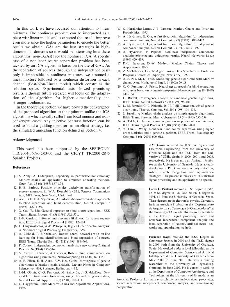
J.M. Gorriz received the B.Sc. in Physics and
Electronic Engineering from the University of
Granada, Spain and the Ph.D. from the Uni-
versity of Cadiz, Spain in 2000, 2001, and 2003,
respectively. He is currently an Assistant Profes-
sor at the University of Granada. He is actually
developing a Ph.D. in voice activity detection,
robust speech recognition and optimization
strategies. His present interests are in statistical
signal processing and its applications to speech.
Carlos G. Puntonet received a B.Sc. degree in 1982,
an M.Sc. degree in 1986 and his Ph.D. degree in
1994, all from the University of Granada, Spain.
These degrees are in electronics physics. Currently,
he is an Associate Professor at the ‘‘Departamento
de Arquitectura y Tecnologıa de Computadores’’ at
the University of Granada. His research interests lie
in the fields of signal processing, linear and
nonlinear independent component analysis and
blind separation of sources, artificial neural net-
works and optimization methods.
Fernando Rojas received the B.Sc. Degree in
Computer Science in 2000 and the Ph.D. degree
in 2004 both from the University of Granada,
Spain. He worked under a local fellowship at the
Department of Computer Science and Artificial
Intelligence at the University of Granada from
May 2000 to June 2001. He was a visiting
researcher at the University of Regensburg,
Germany, in June 2002. He is currently working
at the Department of Computer Architecture and
Technology, at the University of Granada as an
Associate Professor. His main research interests include signal processing,
source separation, independent component analysis, and evolutionary
computation.

ARTICLE IN PRESSJ.M. Gorriz et al. / Neurocomputing 69 (2006) 1442–1457 1457
Ruben Martin-Clemente was born on August 9,
1973, in Cordoba, Spain. He received the M.Sc.
and Ph.D. degrees in Telecommunications en-
gineering from the University of Seville, Seville,
Spain, in 1996 and 2000, respectively.
He is currently an Associate Professor with the
Department of Signal Theory and Communica-
tions, University of Seville. His research interests
include blind signal separation, higher order
statistics and statistical signal processing.
Susana Hornillo-Mellado received the M.Sc.
degree in Telecommunications Engineering from
the University of Seville, Seville, Spain, in 2001.
She is currently pursuing the Ph.D. degree in
Telecommunications Engineering with the
Department of Signal Theory and Communica-
tions, University of Seville. Her research interests
include blind signal separation, independent
component analysis and image processing.
E.W. Lang received his physics diploma with
excellent grade in 1977 and his Ph.D. in physics
(summa cum laude) in 1980 and habilitated in
Biophysics in 1988 at the University of Regens-
burg. He is apl. Professor of Biophysics at the
University of Regensburg. He is currently associ-
ate editor of Neurocomputing and Neural
Information Processing—Letters and Reviews.
His current research interests focus mainly on
machine learning and include biomedical signal
processing, independent component analysis and
blind source separation, neural networks for classification and pattern
recognition as well as stochastic process limits in queuing applications.