2005 IEEE Workshop on Applications of Signal Processing to Audio and Acoustics October 16-19, 2005, New Paltz, NY

BLIND SOURCE SEPARATION OF 3-D LOCATED MANY SPEECH SIGNALS

Ryo Mukai Hiroshi Sawada Shoko Araki Shoji Makino

NTT Communication Science Laboratories, NTT Corporation

2–4 Hikaridai, Seika-cho, Soraku-gun, Kyoto 619–0237, Japan

ryo@cslab.kecl.ntt.co.jp

http://www.kecl.ntt.co.jp/icl/signal/mukai/

ABSTRACT

This paper presents a prototype system for Blind Source

Separation (BSS) of many speech signals and describes the

techniques used in the system. Our system uses 8 micro-

phones located at the vertexes of a 4cm×4cm×4cm cube

and has the ability to separate signals distributed in three-

dimensional space. The mixed signals observed by the mi-

crophone array are processed by Independent Component

Analysis (ICA) in the frequency domain and separated into

a given number of signals (up to 8). We carried out exper-

iments in an ordinary office and obtained more than 20 dB

of SIR improvement.

1. INTRODUCTION

The Blind Source Separation (BSS) [1] of audio signals hasa wide range of applications. In most realistic applications,the number of source signals is large, and the signals aremixed in a convolutive manner with reverberations. Inde-pendent component analysis (ICA) [2] is one of the mainstatistical methods used for BSS. It is theoretically possibleto solve the BSS problem with a large number of sources byICA, if we assume that the number of sensors is equal to orgreater than the number of source signals. However, thereare many practical difficulties. Although many studies havebeen undertaken on BSS in a reverberant environment [3],most of them have assumed two source signals, and only afew studies have dealt with more than two source signals.

In this paper, we present techniques for the BSS of manyspeech signals distributed in three-dimensional space and aprototype system that we have developed. In our previouswork [4], we described the separation of six source signalsconsisting of simulated data, i.e. signals made by convolv-ing impulse responses. In contrast, this prototype systemperforms an on-the-spot BSS of live recorded signals. Thispaper is an extended version of our previous work [5].

2. FREQUENCY DOMAIN BLIND SOURCESEPARATION

There are two major approaches to solving the convolutiveBSS problem. The first is the time domain approach, whereICA is applied directly to the convolutive mixture model[6, 7, 8]. The time domain approach incurs considerable

W(f )

DOAestimation

Separationmatrix

Direction-of-arrival (DOA) offrequency components

ICAFrequency

domain

x(t)

Mixedsignals

Timedomain

f

Separatedsignalsy(t)

Separation filter

STFT IDFT

P(f) D(f)

Permutation

w(l)

Scaling

Figure 1: Flow of frequency domain BSS

computational cost, and it is difficult to obtain a solution ina practical time when the number of source signals is large.

The other approach is frequency domain BSS, whereICA is applied to multiple instantaneous mixtures in the fre-quency domain [9, 10, 11]. This approach takes much lesscomputation time than time domain BSS.

2.1. ICA in frequency domain

When N source signals are s1(t), ..., sN (t) and the signalsobserved by M sensors are x1(t), ..., xM (t), the mixingmodel can be described by

xj(t) =∑N

i=1

∑l hji(l)si(t − l), (1)

where hji(l) is the impulse response from source i to sensorj. The separation system typically consists of a set of FIRfilters wkj(l) of length L designed to produce N separatedsignals y1(t), ..., yN (t), and it is described as:

yk(t) =∑M

j=1

∑L−1l=0 wkj(l)xj(t − l). (2)

Figure 1 shows the flow of BSS in the frequency do-main. Each convolutive mixture in the time domain is con-verted into multiple instantaneous mixtures in the frequencydomain. By using a short-time discrete Fourier transform(DFT), the mixing model is approximated as:

x(f, m) = H(f)s(f, m), (3)

where f denotes the frequency, m is the frame index,s(f, m) = [s1(f, m), ..., sN (f, m)]T is the vector ofthe source signals in the frequency bin f , x(f, m) =[x1(f, m), ..., xM (f, m)]T is the vector of the observed sig-nals, and H(f) is a matrix consisting of the frequency re-

90-7803-9154-3/05/$20.00 ©2005 IEEE

2005 IEEE Workshop on Applications of Signal Processing to Audio and Acoustics October 16-19, 2005, New Paltz, NY

θi,jj′

si

pj

pj′ai

Figure 2: Direction of source i relative to sensor pair j and

j′

si

ai

v1

v2

v3

θi,13

θi,21θi,24

1

4

3

2

j(1)j′(1) = 13, j(2)j′(2) = 24, j(3)j′(3) = 21

Index of sensor pairs

Figure 3: Solving ambiguity of estimated DOAs

sponses Hji(f) from source i to sensor j. The separationprocess can be formulated in each frequency bin as:

y(f, m) = W(f)x(f, m), (4)

where y(f, m) = [y1(f, m), ..., yN (f, m)]T is the vector ofthe separated signals, and W(f) represents the separationmatrix. Therefore, we can apply an ordinary (instantaneous)ICA algorithm to each frequency bin and calculate the sep-aration matrices. W(f) is determined so that the elementsof y(f, m) become mutually independent for each f .

The ICA solution suffers from scaling and permutationambiguities. This is because that if W(f) is a solution, thenD(f)P(f)W(f) is also a solution, where D(f) is a diago-nal complex valued scaling matrix, and P(f) is an arbitrarypermutation matrix. There is a simple and reasonable solu-tion for the scaling problem:

D(f) = diag{[P(f)W(f)]−1}, (5)

which is obtained by the minimal distortion principle(MDP) [12] or the projection back method [13], and wecan use it. On the other hand, the permutation problem iscomplicated, especially when the number of source signalsis large. Before constructing a separation filter in the timedomain, we have to align the permutation so that each chan-nel contains frequency components from one source signal.The time domain filters are obtained by the inverse discreteFourier transform of frequency domain separation matrices.

2.2. DOA estimation using ICA solution

The frequency response matrix H(f) is closely related tothe locations of the sources and sensors. If a separation ma-trix W(f) is calculated successfully and it extracts sourcesignals with a scaling ambiguity, there is a diagonal ma-trix D(f), and D(f)W(f)H(f) = I holds. Because ofthe scaling ambiguity, we cannot obtain H(f) simply from

the ICA solution W(f). However, the ratio of elements inthe same column Hji(f)/Hj′i(f) is invariable in relation toD(f), and is given by

Hji(f)

Hj′i(f)=

[W−1(f)D−1(f)]ji

[W−1(f)D−1(f)]j′i=

[W−1(f)]ji

[W−1(f)]j′i, (6)

where [·]ji denotes the ji-th element of the matrix.

We can estimate the DOA of a source signal by usingthis invariant [4]. With a far-field model, a frequency re-sponse is formulated as:

Hji(f) = e2πfc−1a

Ti pj , (7)

where c is the wave propagation speed, ai is a unit vectorthat points to the direction of source i (absolute DOA), andpj represents the location of sensor j. According to thismodel, we have

Hji(f)/Hj′i(f) = e2πfc−1a

Ti (pj−pj′ ) (8)

= e2πfc−1‖pj−pj′‖ cos θi,jj′ (f), (9)

where θi,jj′ (f) is the direction of source i relative to thesensor pair j and j ′ (relative DOA). Figure 2 shows the re-lation of the absolute DOA and the relative DOA. By usingthe argument of (9) and (6), we can estimate:

θi,jj′ (f) = arccosarg(Hji/Hj′i)

2πfc−1‖(pj − pj′ )‖

= arccosarg([W−1]ji/[W−1]j′i)

2πfc−1‖(pj − pj′ )‖. (10)

θi,jj′ (f) is estimated for each frequency bin f , but we omitthe argument f to simplify the notation in the following de-scription.

The DOA estimation involves certain ambiguities.When we use only one pair of sensors or a linear array, the

estimated θi,jj′ determines a cone rather than a direction.This ambiguity can be solved by using multiple sensor pairs(Fig. 3). If we use sensor pairs that have different axis direc-tions, we can estimate cones with various vertex angles for

one source direction. If the relative DOA θi,jj′ is estimatedwithout any error, the absolute DOA ai satisfies:

(pj − pj′ )T ai

‖pj − pj′‖= cos θi,jj′ . (11)

When we use L sensor pairs whose indexes arej(l)j′(l)(1 ≤ l ≤ L), ai is given by the solution of thefollowing equation:

Vai = ci, (12)

where V�= (v1, ...,vL)T

, vl�=

pj(l)−pj′(l)

‖pj(l)−pj′(l)‖is a normal-

ized axis, and ci�= [cos(θi,j(1)j′(1)), ..., cos(θi,j(L)j′(L))]

T .Sensor pairs should be selected so that rank(V) ≥ 3 if thepotential source locations are three-dimensional.

In a practical situation, θi,j(l)j′(l) has an estimation er-ror, and (12) has no exact solution. Thus we adopt an opti-mal solution by employing certain criteria such as:

ai = argmina

||Va − ci|| (subject to ||a|| = 1) (13)

This can be solved approximately by using the Moore-

10

2005 IEEE Workshop on Applications of Signal Processing to Audio and Acoustics October 16-19, 2005, New Paltz, NY

x y

z

-1

-0.5

0

0.5

1

-0.5

0

0.5

-1

-0.5

0

0.5

1

-1

-0.5

0

0.5

1

-0.5

0

0.5

-1

-0.5

0

0.5

1

x y

z

Figure 4: Estimated DOAs of frequency components

(above) and clustered result (below)

Penrose pseudo-inverse V+ �= (VT V)−1VT , and we

have:

ai ≈V+ci

||V+ci||. (14)

Accordingly, we can determine a unit vector ai pointing tothe direction of source si.

Figure 4 shows an example of a DOA estimation re-sult. Each point plotted on a unit sphere denotes the es-timated DOA of a frequency component in one frequencybin. The points can be clustered by using an ordinary clus-tering method such as the k-means algorithm [14], then theDOAs of source signals are given as the centroids of theclusters. This information is useful for solving the permuta-tion problem.

2.3. Permutation solver using DOA and correlation

This subsection outlines the procedure for permutationalignment by integrating a DOA based approach and a cor-relation approach. This procedure has been detailed in [11],and consists of the following steps:

1. Cluster separated frequency components yk(f, m) for

all k and all f by using the estimated DOA, and de-cide the permutations at certain frequencies where theconfidence of DOA estimation is sufficiently high.

2. Decide the permutations to maximize the sum of theinter-frequency correlation of the separated signals.The correlation should be calculated for the ampli-tude |yk(f, m)| or (log-scaled) power |yk(f, m)|2 in-stead of the raw complex-valued signals yk(f, m),since the correlation of raw signals would be verylow because of the short-time DFT property. The sumof the correlations between |yk(f, m)| and |yk(g, m)|within distance δ (i.e. |f − g| < δ) is used as a cri-terion. The permutations are decided for frequencieswhere the criterion gives a clear-cut decision.

3. Calculate the correlations between |yk(f, m)| and itsharmonics |yk(g, m)| (g = 2f, 3f, 4f, ...), and decidethe permutations that maximize the sum of the corre-lations. The permutations are decided for frequencieswhere the correlation among harmonics is sufficientlyhigh.

4. Decide the permutations for the remaining frequen-cies based on neighboring correlations.

The DOA estimation suffers from errors in a reverberantenvironment and the classification according to the DOA isinconsistent in some frequency bins. The correlation basedmethod is not robust since a misalignment at one frequencybin causes consecutive misalignments. The main advantageof the integrated method is that it does not cause a largemisalignment as long as the permutations fixed by the DOAbased approach are correct. Moreover, the correlation part(steps 2, 3 and 4) compensates for the lack of preciseness ofthe DOA based approach. The correlation part consists ofthree steps for two reasons. First, the harmonics part (step3) works well if most of the other permutations are fixed.Second, the method becomes more robust by quitting thestep 2 if there is no clear-cut decision. With this structure,we can avoid fixing the permutations for consecutive fre-quencies without high confidence. This integrated methodis effective when the number of source signals is large.

2.4. Spectral smoothing with error minimization

Frequency domain BSS is influenced by the circularity ofthe discrete frequency representation. This causes a prob-lem when we convert separation matrices in the frequencydomain into a separation filter in the time domain. Thisproblem is not apparent when there are two sources, how-ever it is crucial when the number of source signals exceedstwo. Our technique for solving this problem involves spec-tral smoothing of separation filters by using a window thattapers smoothly to zero at each end. The direct applicationof windowing changes the frequency responses for separa-tion obtained by ICA and causes an error. Therefore, we ad-just the frequency responses before windowing so that theerror is minimized. The procedure is presented in detail in[15].

11

2005 IEEE Workshop on Applications of Signal Processing to Audio and Acoustics October 16-19, 2005, New Paltz, NY

Note PC

A/D converter

D/A converter

1

2

3

4

6

6 loudspeakers

5

4cm

8 omnidirectional

microphones

4cm

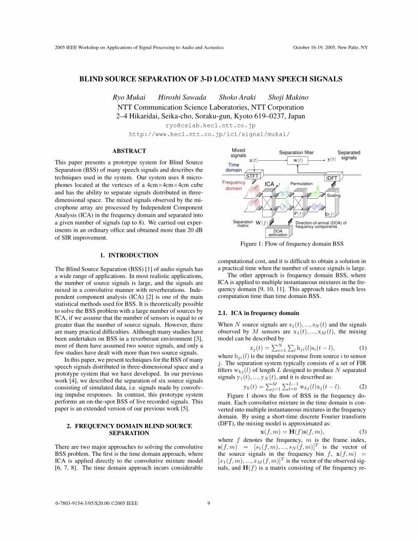
Figure 5: Prototype system and experimental settings

Table 1: Specifications of prototype systemMicrophone 8 omni-directional microphones

Sampling rate 8 kHzFrame length 2048 points (256 ms)

Frame shift 512 points (64 ms)

ICA algorithm FastICA + Infomax (complex valued)CPU Intel Pentium M (2.0 GHz)

Coding MATLAB + C

Computation time 25 s for 6 sources 8 s data

3. PROTOTYPE SYSTEM AND EXPERIMENTS

We have developed a prototype using the techniques de-scribed above. Our system uses 8 microphones located atthe vertexes of a 4cm×4cm×4cm cube and has the abil-ity to separate six signals distributed in three-dimensionalspace (Fig. 5). The system specifications are summarized inTable 1. This system is implemented in software (MATLAB+ C) and needs no special hardware except for an A/D con-verter. We calculated W by using a complex-valued versionof FastICA [16] and improved it further by using InfoMax[17] combined with the natural gradient whose nonlinearfunction is based on the polar coordinate [18].

We carried out experiments in an ordinary office andevaluated the Signal to Interference Ratio (SIR) perfor-mance. The source locations are shown in Fig. 5. Wecalculated the separation filter by using live recorded mix-tures, and evaluated the SIRs by using individually activatedsource signals. The experimental results are shown in Ta-ble 2. We obtained good separation performance in spite ofthe very low input SIR. The average SIR improvement wasmore than 20 dB.

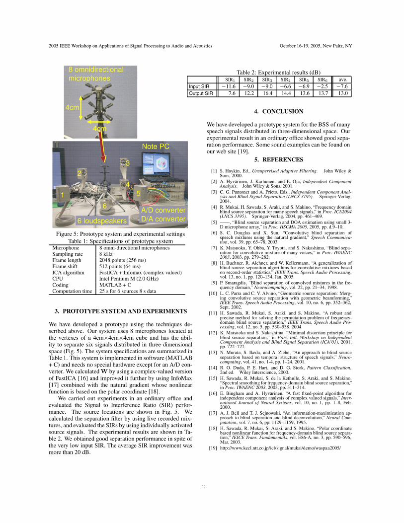
Table 2: Experimental results (dB)SIR1 SIR2 SIR3 SIR4 SIR5 SIR6 ave.

Input SIR −11.6 −9.0 −9.0 −6.6 −6.9 −2.5 −7.6

Output SIR 7.6 12.2 16.4 14.4 13.6 13.7 13.0

4. CONCLUSION

We have developed a prototype system for the BSS of manyspeech signals distributed in three-dimensional space. Ourexperimental result in an ordinary office showed good sepa-ration performance. Some sound examples can be found onour web site [19].

5. REFERENCES

[1] S. Haykin, Ed., Unsupervised Adaptive Filtering. John Wiley &Sons, 2000.

[2] A. Hyvarinen, J. Karhunen, and E. Oja, Independent ComponentAnalysis. John Wiley & Sons, 2001.

[3] C. G. Puntonet and A. Prieto, Eds., Independent Component Anal-ysis and Blind Signal Separation (LNCS 3195). Springer-Verlag,2004.

[4] R. Mukai, H. Sawada, S. Araki, and S. Makino, “Frequency domainblind source separation for many speech signals,” in Proc. ICA2004(LNCS 3195). Springer-Verlag, 2004, pp. 461–469.

[5] ——, “Blind source separation and DOA estimation using small 3-D microphone array,” in Proc. HSCMA 2005, 2005, pp. d.9–10.

[6] S. C. Douglas and X. Sun, “Convolutive blind separation ofspeech mixtures using the natural gradient,” Speech Communica-tion, vol. 39, pp. 65–78, 2003.

[7] K. Matsuoka, Y. Ohba, Y. Toyota, and S. Nakashima, “Blind sepa-ration for convolutive mixture of many voices,” in Proc. IWAENC2003, 2003, pp. 279–282.

[8] H. Buchner, R. Aichner, and W. Kellermann, “A generalization ofblind source separation algorithms for convolutive mixtures basedon second-order statistics,” IEEE Trans. Speech Audio Processing,vol. 13, no. 1, pp. 120–134, Jan. 2005.

[9] P. Smaragdis, “Blind separation of convolved mixtures in the fre-quency domain,” Neurocomputing, vol. 22, pp. 21–34, 1998.

[10] L. C. Parra and C. V. Alvino, “Geometric source separation: Merg-ing convolutive source separation with geometric beamforming,”IEEE Trans. Speech Audio Processing, vol. 10, no. 6, pp. 352–362,Sept. 2002.

[11] H. Sawada, R. Mukai, S. Araki, and S. Makino, “A robust andprecise method for solving the permutation problem of frequency-domain blind source separation,” IEEE Trans. Speech Audio Pro-cessing, vol. 12, no. 5, pp. 530–538, 2004.

[12] K. Matsuoka and S. Nakashima, “Minimal distortion principle forblind source separation,” in Proc. Intl. Workshop on IndependentComponent Analysis and Blind Signal Separation (ICA’01), 2001,pp. 722–727.

[13] N. Murata, S. Ikeda, and A. Ziehe, “An approach to blind sourceseparation based on temporal structure of speech signals,” Neuro-computing, vol. 41, no. 1-4, pp. 1–24, 2001.

[14] R. O. Duda, P. E. Hart, and D. G. Stork, Pattern Classification,2nd ed. Wiley Interscience, 2000.

[15] H. Sawada, R. Mukai, S. de la Kethulle, S. Araki, and S. Makino,“Spectral smoothing for frequency-domain blind source separation,”in Proc. IWAENC 2003, 2003, pp. 311–314.

[16] E. Bingham and A. Hyvarinen, “A fast fixed-point algorithm forindependent component analysis of complex valued signals,” Inter-national Journal of Neural Systems, vol. 10, no. 1, pp. 1–8, Feb.2000.

[17] A. J. Bell and T. J. Sejnowski, “An information-maximization ap-proach to blind separation and blind deconvolution,” Neural Com-putation, vol. 7, no. 6, pp. 1129–1159, 1995.

[18] H. Sawada, R. Mukai, S. Araki, and S. Makino, “Polar coordinatebased nonlinear function for frequency-domain blind source separa-tion,” IEICE Trans. Fundamentals, vol. E86-A, no. 3, pp. 590–596,Mar. 2003.

[19] http://www.kecl.ntt.co.jp/icl/signal/mukai/demo/waspaa2005/

12