bLSM:∗ A General Purpose Log Structured Merge Tree

Russell SearsYahoo! ResearchSanta Clara, CA

Raghu RamakrishnanYahoo! ResearchSanta Clara, CA

ABSTRACTData management workloads are increasingly write-intensiveand subject to strict latency SLAs. This presents a dilemma:Update in place systems have unmatched latency but poorwrite throughput. In contrast, existing log structured tech-niques improve write throughput but sacrifice read perfor-mance and exhibit unacceptable latency spikes.

We begin by presenting a new performance metric: readfanout, and argue that, with read and write amplification,it better characterizes real-world indexes than approachessuch as asymptotic analysis and price/performance.

We then present bLSM, a Log Structured Merge (LSM)tree with the advantages of B-Trees and log structured ap-proaches: (1) Unlike existing log structured trees, bLSMhas near-optimal read and scan performance, and (2) itsnew “spring and gear” merge scheduler bounds write latencywithout impacting throughput or allowing merges to blockwrites for extended periods of time. It does this by ensuringmerges at each level of the tree make steady progress with-out resorting to techniques that degrade read performance.

We use Bloom filters to improve index performance, andfind a number of subtleties arise. First, we ensure reads canstop after finding one version of a record. Otherwise, fre-quently written items would incur multiple B-Tree lookups.Second, many applications check for existing values at in-sert. Avoiding the seek performed by the check is crucial.

Categories and Subject DescriptorsH.3.2 [Information Storage]: File organization

General TermsAlgorithms, Performance

KeywordsLog Structured Merge tree, merge scheduling, read fanout,read amplification, write amplification

∗Pronounced “Blossom”

Permission to make digital or hard copies of all or part of this work forpersonal or classroom use is granted without fee provided that copies arenot made or distributed for profit or commercial advantage and that copiesbear this notice and the full citation on the first page. To copy otherwise, torepublish, to post on servers or to redistribute to lists, requires prior specificpermission and/or a fee.SIGMOD ’12, May 20–24, 2012, Scottsdale, Arizona, USA.Copyright 2012 ACM 978-1-4503-1247-9/12/05 ...$10.00.

1. INTRODUCTIONModern web services rely upon two types of storage for

small objects. The first, update-in-place, optimizes for ran-dom reads and worst case write latencies. Such stores areused by interactive, user facing portions of applications. Thesecond type is used for analytical workloads and emphasizeswrite throughput and sequential reads over latency or ran-dom access. This forces applications to be broken into “fast-path” processing, and asynchronous analytical tasks.

This impacts end-users (e.g., it may take hours for ma-chine learning models to react to users’ behavior), and forcesoperators to manage redundant storage infrastructures.

Such limitations are increasingly unacceptable. Cloudcomputing, mobile devices and social networking write dataat unprecedented rates, and demand that updates be syn-chronously exposed to devices, users and other services. Un-like traditional write-heavy workloads, these applicationshave stringent latency SLAs.

These trends have two immediate implications at Yahoo!.First, in 2010, typical low latency workloads were 80-90%reads. Today the ratio is approaching 50%, and the shiftfrom reads to writes is expected to accelerate in 2012. Thesetrends are driven by applications that ingest event logs (suchas user clicks and mobile device sensor readings), and latermine the data by issuing long scans, or targeted point queries.

Second, the need for performant index probes in writeoptimized systems is increasing. bLSM is designed to beused as backing storage for PNUTS, our geographically-distributed key-value storage system [10], and Walnut, ournext-generation elastic cloud storage system [9].

Historically, limitations of log structured indexes have pre-sented a trade off. Update-in-place storage provided su-perior read performance and predictability for writes; log-structured trees traded this for improved write throughput.This is reflected in the infrastructures of companies such asYahoo!, Facebook [6] and Google, each of which employsInnoDB and either HBase [1] or BigTable [8] in production.

This paper argues that, with appropriate tuning and ourmerge scheduler improvements, LSM-trees are ready to sup-plant B-Trees in essentially all interesting application sce-narios. The two workloads we describe above, interactiveand analytical, are prime examples: they cover most appli-cations, and, as importantly, are the workloads that most-frequently push the performance envelope of existing sys-tems. Inevitably, switching from B-Trees to LSM-Trees en-tails a number of tradeoffs, and B-Trees still outperform logstructured approaches in a number of corner cases. Theseare summarized in Table 1.

217

Operation Our bLSM-Tree B-Tree LevelDB

Point lookup (seeks) 1 §3.1.1 1 §2.2 O(log(n))Read modify write (seeks) 1 §2.3 2 §2.2 O(log(n))

Apply delta to record (seeks) 0 §2.3 2 §2.2 0Insert or overwrite (seeks) 0 §3.1.2 2 §2.2 0

Short (≤ 1 page) scans (seeks) 2 §3.3 1 §2.2 O(log(n))Long (N page) scans (seeks) 2 §3.3 Up to N §2.2 O(log(n))

Uniform random insert latency Bounded §4.1-§4.3 Bounded §2.2 UnboundedWorst-case insert latency Unbounded See §4.2.2 for a fix Bounded §2.2 Unbounded

Table 1: Summary of results. bLSM-Trees outperform B-Trees and LSM-Tees in most interesting scenarios.

12

3 4

51

2

34

5

A

BC

D E

AE

D C

BA

E

DC

B

Applicationwrites

C0:C1merge

C1':C2merge

% full

C0 C1 C1'

in progress= [1-5]

out progress= [A-E]

C2

in progress= [A-E]

Applicationreads

1

2 3 4

BloomFilters

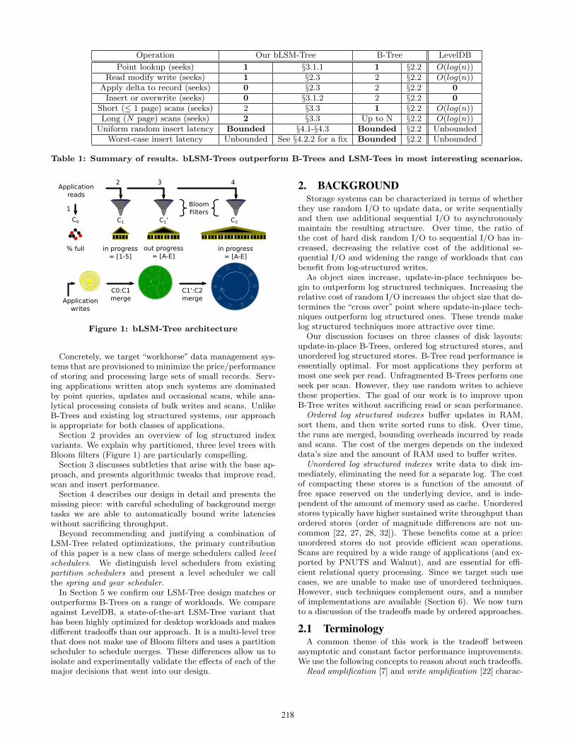
Figure 1: bLSM-Tree architecture

Concretely, we target “workhorse” data management sys-tems that are provisioned to minimize the price/performanceof storing and processing large sets of small records. Serv-ing applications written atop such systems are dominatedby point queries, updates and occasional scans, while ana-lytical processing consists of bulk writes and scans. UnlikeB-Trees and existing log structured systems, our approachis appropriate for both classes of applications.

Section 2 provides an overview of log structured indexvariants. We explain why partitioned, three level trees withBloom filters (Figure 1) are particularly compelling.

Section 3 discusses subtleties that arise with the base ap-proach, and presents algorithmic tweaks that improve read,scan and insert performance.

Section 4 describes our design in detail and presents themissing piece: with careful scheduling of background mergetasks we are able to automatically bound write latencieswithout sacrificing throughput.

Beyond recommending and justifying a combination ofLSM-Tree related optimizations, the primary contributionof this paper is a new class of merge schedulers called levelschedulers. We distinguish level schedulers from existingpartition schedulers and present a level scheduler we callthe spring and gear scheduler.

In Section 5 we confirm our LSM-Tree design matches oroutperforms B-Trees on a range of workloads. We compareagainst LevelDB, a state-of-the-art LSM-Tree variant thathas been highly optimized for desktop workloads and makesdifferent tradeoffs than our approach. It is a multi-level treethat does not make use of Bloom filters and uses a partitionscheduler to schedule merges. These differences allow us toisolate and experimentally validate the effects of each of themajor decisions that went into our design.

2. BACKGROUNDStorage systems can be characterized in terms of whether

they use random I/O to update data, or write sequentiallyand then use additional sequential I/O to asynchronouslymaintain the resulting structure. Over time, the ratio ofthe cost of hard disk random I/O to sequential I/O has in-creased, decreasing the relative cost of the additional se-quential I/O and widening the range of workloads that canbenefit from log-structured writes.

As object sizes increase, update-in-place techniques be-gin to outperform log structured techniques. Increasing therelative cost of random I/O increases the object size that de-termines the “cross over” point where update-in-place tech-niques outperform log structured ones. These trends makelog structured techniques more attractive over time.

Our discussion focuses on three classes of disk layouts:update-in-place B-Trees, ordered log structured stores, andunordered log structured stores. B-Tree read performance isessentially optimal. For most applications they perform atmost one seek per read. Unfragmented B-Trees perform oneseek per scan. However, they use random writes to achievethese properties. The goal of our work is to improve uponB-Tree writes without sacrificing read or scan performance.

Ordered log structured indexes buffer updates in RAM,sort them, and then write sorted runs to disk. Over time,the runs are merged, bounding overheads incurred by readsand scans. The cost of the merges depends on the indexeddata’s size and the amount of RAM used to buffer writes.

Unordered log structured indexes write data to disk im-mediately, eliminating the need for a separate log. The costof compacting these stores is a function of the amount offree space reserved on the underlying device, and is inde-pendent of the amount of memory used as cache. Unorderedstores typically have higher sustained write throughput thanordered stores (order of magnitude differences are not un-common [22, 27, 28, 32]). These benefits come at a price:unordered stores do not provide efficient scan operations.Scans are required by a wide range of applications (and ex-ported by PNUTS and Walnut), and are essential for effi-cient relational query processing. Since we target such usecases, we are unable to make use of unordered techniques.However, such techniques complement ours, and a numberof implementations are available (Section 6). We now turnto a discussion of the tradeoffs made by ordered approaches.

2.1 TerminologyA common theme of this work is the tradeoff between

asymptotic and constant factor performance improvements.We use the following concepts to reason about such tradeoffs.

Read amplification [7] and write amplification [22] charac-

218

terize the cost of reads and writes versus optimal schemes.We measure read amplification in terms of seeks, since atleast one random read is required to access an uncached pieceof data, and the seek cost generally dwarfs the transfer cost.In contrast, writes can be performed using sequential I/O,so we express write amplification in terms of bandwidth.By convention, our computations assume worst-case accesspatterns and optimal caching policies.

read amplification = worst case seeks per index probe

write amplification =total seq. I/O for object

object size

Write amplification includes both the synchronous cost ofthe write, and the cost of deferred merges or compactions.

Given a desired read amplification, we can compute theread fanout (our term) of an index. The read fanout is theratio of the data size to the amount of RAM used by theindex. To simplify our calculations, we linearly approximateread fanout by only counting the cost of storing the bottom-most layer of the index pages in RAM. Main memory hasgrown to the point where read amplifications of one (or evenzero) are common (Appendix A). Here, we focus on readfanouts with a read amplification of one.

2.2 B-TreesAssuming that keys fit in memory, B-Trees provide opti-

mal random reads; they perform a single disk seek each timean uncached piece of data is requested. In order to performan update, B-Trees read the old version of the page, modifyit, and asynchronously write the modification to disk. Thisworks well if data fits in memory, but performs two disk seekswhen the data to be modified resides on disk. Update-in-place hashtables behave similarly, except that they give upthe ability to perform scans in order to make more efficientuse of RAM.

Update in place techniques’ effective write amplificationsdepend on the underlying disk. Modern hard disks transfer100-200MB/sec, and have mean access times over 5ms. Onethousand byte key value pairs are fairly common; it takes the

disk 103

108seconds = 10us to write such a tuple sequentially.

Performing two seeks takes a total of 10ms, giving us a writeamplification of approximately 1000.

Appendix A applies these calculations and a variant of thefive minute rule [15] to estimate the memory required for aread amplification of one with various disk technologies.

2.3 LSM-TreesThis section begins by describing the base LSM-Tree al-

gorithm, which has unacceptably high read amplification,cannot take advantage of write locality, and can stall appli-cation writes for arbitrary periods of time. However, LSM-Tree write amplification is much lower than that of a B-Tree,and the disadvantages are avoidable.

Write skew can be addressed with tree partitioning, whichis compatible with the other optimizations. However, wefind that long write pauses are not adequately addressed byexisting proposals or by state-of-the-art implementations.

2.3.1 Base algorithmLSM-Trees consist of a number of append-only B-Trees

and a smaller update-in-place tree that fits in memory. Wecall the in-memory tree C0. Repeated scans and merges of

these trees are used to spill memory to disk, and to boundthe number of trees consulted by each read.

The trees are stored in key order on disk and the in-memory tree supports efficient ordered scans. Therefore,each merge can be performed in a single pass. In the ver-sion of the algorithm we implement (Figure 1), the numbertrees is constant. The on-disk trees are ordered by freshness;the newest data is in C0. Newly merged trees replace thehigher-numbered of the two input trees. Tree merges arealways performed between Ci and Ci+1.

The merge threads attempt to ensure that the trees in-crease in size exponentially, as this minimizes the amortizedcost of garbage collection. This can be proven in many dif-ferent ways, and stems from a number of observations [25]:

1. Each update moves from tree Ci to Ci+1 at most once.All merge costs are due to such movements.

2. The cost of moving an update is proportional to thecost of scanning the overlapping data range in the large

tree. On average, this cost is Ri =|Ci+1||Ci|

per byte of

data moved.

3. The size of the indexed data is roughly |C0|∗∏N−1

i=0 Ri.

This defines a simple optimization problem in which we varythe Ri in order to minimize the sum of costs (bullet 2) whileholding the index size constant (bullet 3). This optimization

tells us to set each Ri = N−1

√|data||C0|

. It immediately follows

that the amortized cost of insertion is O( N−1√|data|).

Note that the analysis holds for best, average and worst-case workloads. Although LSM-Tree write amplification ismuch lower than B-Trees’ worst case, B-Trees naturally lever-age skewed writes. Skew allows B-Trees to provide muchlower write amplifications than the base LSM-Tree algo-rithm. Furthermore, LSM-Tree lookups and scans performN − 1 times as many seeks as a B-Tree lookup, since (in theworst case), they examine each tree component.

2.3.2 Leveraging write skewAlthough we describe a special case solution in Section 4.2,

partitioning is the best way to allow LSM-Trees to leveragewrite skew [16]. Breaking the LSM-Tree into smaller treesand merging the trees according to their update rates con-centrates merge activity on frequently updated key ranges.

It also addresses one source of write pauses. If the dis-tribution of the keys of incoming writes varies significantlyfrom the existing distribution, then large ranges of the largertree component may be disjoint from the smaller tree. With-out partitioning, merge threads needlessly copy the disjointdata, wasting I/O bandwidth and stalling merges of smallertrees. During these stalls, the application cannot make for-ward progress.

Partitioning can intersperse merges that will quickly con-sume data from the small tree with merges that will slowlyconsume the data, “spreading out” the pause over time. Sec-tions 4.1 and 5 argue and show experimentally that, al-though necessary in some scenarios, such techniques are in-adequate protection against long merge pauses. This con-clusion is in line with the reported behavior of systems withpartition-based merge schedulers, [1, 12, 19] and with pre-vious work, [16] which finds that partitioned and baselineLSM-Tree merges have similar latency properties.

219

With fractional cascading, lookups begin bysearching the index, then check short runs

of data pages at each level of the tree.0 2 4 6 8 10 12 14 16

Data size (multiples of available RAM)

0

1

2

3

4

5

6

Read

am

plifi

cati

on (

seeks

)

Variable R with Bloom Filters (our approach)R=2R=3R=4R=5R=6R=7R=8R=9R=10

0 2 4 6 8 10 12 14 16

Data size (multiples of available RAM)

0

2

4

6

8

10

12

Read

am

plifi

cati

on (

band

wid

th) Variable R with Bloom Filters (our approach)

R=2R=3R=4R=5R=6R=7R=8R=9R=10

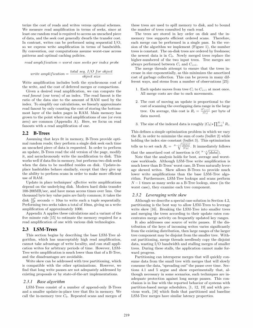
Figure 2: Fractional cascading reduces the cost of lookups from O(log(n)2) to O(log(n)), but mixes keys anddata, increasing read amplification. For our scenarios, Bloom filters’ maximum amplification is 1.03.

3. ALGORITHMIC IMPROVEMENTSWe now present bLSM, our new LSM-Tree variant, which

addresses the LSM-Tree limitations we describe above. Thefirst limitation of LSM-Trees, excessive read amplification,is only partially addressed by Bloom filters, and is closelyrelated to two other issues: exhaustive lookups which need-lessly retrieve multiple versions of a record, and seeks duringinsert. The second issue, write pauses, requires schedulinginfrastructure that is missing from current implementations.

3.1 Reducing read amplificationFractal cascading and Bloom filters both reduce read am-

plification. Fractal cascading reduces asymptotic costs; Bloomfilters instead improve performance by a constant factor.

The Bloom filter approach protects the C1...CN tree com-ponents with Bloom filters. The amount of memory it re-quires is a function of the number of items to be inserted, notthe items’ sizes. Allocating 10 bits per item leads to a 1%false positive rate,1 and is a reasonable tradeoff in practice.Such Bloom filters reduce the read amplification of LSM-Tree point lookups from N to 1+ N

100. Unfortunately, Bloom

Filters do not improve scan performance. Appendix A runsthrough a“typical”application scenario; Bloom filters wouldincrease memory utilization by about 5% in that setting.

Unlike Bloom filters, fractional cascading [18] reduces theasymptotic complexity of write-optimized LSM-Trees. In-stead of varying R, these trees hold R constant and addadditional levels as needed, leading to a logarithmic numberof levels and logarithmic write amplification. Lookups andscans access a logarithmic (instead of constant) number oftree components. Such techniques are used in systems thatmust maintain large number of materialized views, such asthe TokuDB MySQL storage engine [18].

Fractional cascading includes pointers in tree componentleaf pages that point into the leaves of the next largest tree.Since R is constant, the cost of traversing one of these point-ers is also constant. This eliminates the logarithmic factorassociated with performing multiple B-Tree traversals.

The problem with this scheme is that the cascade stepsof the search examine pages that likely reside on disk. Ineffect, it eliminates a logarithmic in-memory overhead byincreasing read amplification by a logarithmic factor.

Figure 2 provides an overview of the lookup process, and

1Bloom filters can claim to contain an item that has notbeen inserted, causing us to unnecessarily examine the disk.

plots read amplification vs. fanout for fractional cascadingand for three-level LSM-Trees with Bloom filters. No settingof R allows fractional cascading to provide reads competitivewith Bloom filters—reducing read amplification to 1 requiresan R large enough to ensure that there is a single on-disktree component. Doing so leads to O(n) write amplifications.Given this, we opt for Bloom filters.

3.1.1 Limiting read amplification for frequently up-dated data

On their own, Bloom filters cannot ensure that read am-plifications are close to 1, since copies of a record (or itsdeltas) may exist in multiple trees. To get maximum readperformance, applications should avoid writing deltas, andinstead write base records for each update.

Our reads begin with the lowest numbered tree compo-nent, continue with larger components in order and stop atthe first base record. Our reads are able to terminate earlybecause they distinguish between base records and deltas,and because updates to the same tuple are placed in treelevels consistent with their ordering. This guarantees thatreads encounter the most recent version first, and has nonegative impact on write throughput. Other systems non-deterministically assign reads to on-disk components, anduse timestamps to infer write ordering. This breaks earlytermination, and can lead to update anomalies [1].

3.1.2 Zero-seek “insert if not exists”One might think that maintaining a Bloom filter on the

largest tree component is a waste; this Bloom filter is by farthe largest in the system, and (since C2 is the last tree to besearched) it only accelerates lookups of non-existent data.It turns out that such lookups are extremely common; theyare performed by operations such as “insert if not exists.”

In Section 5.2, we present performance results for bulkloads of bLSM, InnoDB and LevelDB. Of the three, onlybLSM could efficiently load and check our modest 50GBunordered data set for duplicates. “Insert if not exists” is awidely used primitive; lack of efficient support for it rendershigh-throughput writes useless in many environments.

3.2 Dealing with write pausesRegardless of optimizations that improve read amplifica-

tion and leverage write skew, index implementations thatimpose long, sporadic write outages on end users are notparticularly practical. Despite the lack of good solutions,

220

LSM-Trees are regularly put into production. We describeworkarounds that are used in practice here.

At the index level, the most obvious solution (other thanunplanned downtime) is to introduce extra C1 componentswhenever C0 is full and the C1 merge has not yet com-pleted [13]. Bloom filters reduce the impact of extra trees,but this approach still severely impacts scan performance.Systems such as HBase allow administrators to temporarilydisable compaction, effectively implementing this policy [1].As we mentioned above, applications that do not requireperformant scans would be better off with an unordered logstructured index.

Passing the problem off to the end user increases opera-tions costs, and can lead to unbounded space amplification.However, merges can be run during off-peak periods, increas-ing throughput during peak hours. Similarly, applicationsthat index data according to insertion time end up writingdata in “almost sorted” order, and are easily handled by ex-isting merge strategies, providing a stop-gap solution untilmore general purposes systems become available.

Another solution takes partitioning to its logical extreme,creating partitions so small that even worst case merges in-troduce short pauses. This is the technique taken by Parti-tioned Exponential Files [16] and LevelDB [12]. Our exper-imental results show that this, on its own, is inadequate. Inparticular, with uniform inserts and a “fair” partition sched-uler, each partition would simultaneously evolve into thesame bad state described in Figure 4. At best, this wouldlead to a throughput collapse (instead of a complete cessa-tion of application writes).

Obviously, we find each of these approaches to be un-acceptable. Section 4.1 presents our approach to mergescheduling. After presenting a simple merge scheduler, wedescribe an optimization and extensions designed to allowour techniques to coexist with partitioning.

3.3 Two-seek scansScan operations do not benefit from Bloom filters and

must examine each tree component. This, and the impor-tance of delta-based updates led us to bound the number ofon-disk tree components. bLSM currently has three compo-nents and performs three seeks. Indeed, Section 5.6 presentsthe sole experiment in which InnoDB outperforms bLSM: ascan-heavy workload.

We can further improve short-scan performance in con-junction with partitioning. One of the three on-disk compo-nents only exists to support the ongoing merge. In a systemthat made use of partitioning, only a small fraction of thetree would be subject to merging at any given time. Theremainder of the tree would require two seeks per scan.

4. BLSMAs the previous sections explained, scans and reads are

crucial to real-world application performance. As we de-cided which LSM-Tree variants and optimizations to use inour design, our first priority was to outperform B-Trees inpractice. Our second concern was to do so while providingasymptotically optimal LSM-Tree write throughput. Theprevious section outlined the changes we made to the baseLSM-Tree algorithm in order to meet these requirements.

Figure 1 presents the architecture of our system. We usea three-level LSM-Tree and protect the two on-disk levelswith Bloom filters. We have not yet implemented parti-

A-F

G-M

N-Q

R-ZDeci

de w

hic

h k

ey

part

itio

n t

o m

erg

e

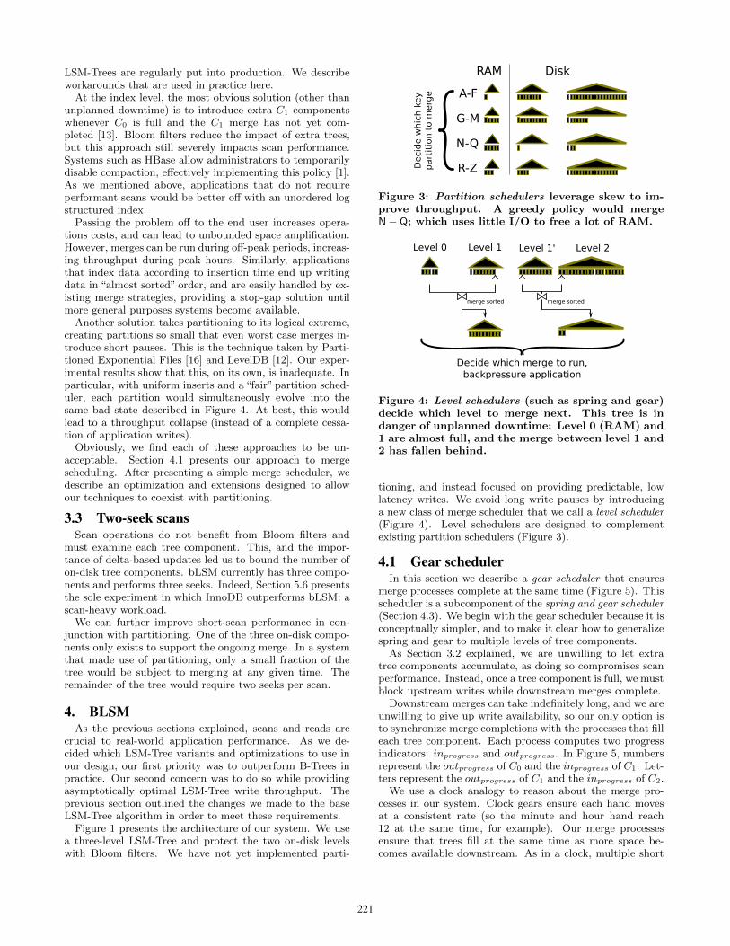
RAM Disk

Figure 3: Partition schedulers leverage skew to im-prove throughput. A greedy policy would mergeN− Q; which uses little I/O to free a lot of RAM.

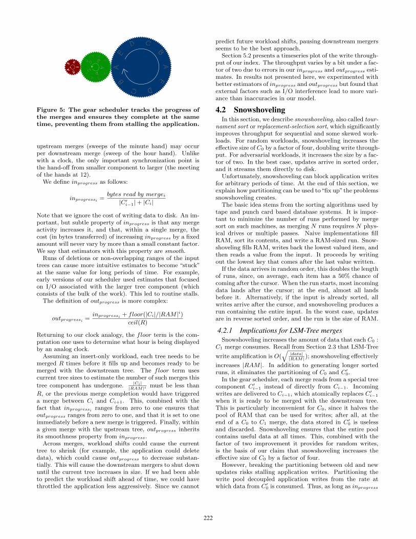
Level 1 Level 1' Level 2Level 0

Decide which merge to run,backpressure application

merge sorted merge sorted

Figure 4: Level schedulers (such as spring and gear)decide which level to merge next. This tree is indanger of unplanned downtime: Level 0 (RAM) and1 are almost full, and the merge between level 1 and2 has fallen behind.

tioning, and instead focused on providing predictable, lowlatency writes. We avoid long write pauses by introducinga new class of merge scheduler that we call a level scheduler(Figure 4). Level schedulers are designed to complementexisting partition schedulers (Figure 3).

4.1 Gear schedulerIn this section we describe a gear scheduler that ensures

merge processes complete at the same time (Figure 5). Thisscheduler is a subcomponent of the spring and gear scheduler(Section 4.3). We begin with the gear scheduler because it isconceptually simpler, and to make it clear how to generalizespring and gear to multiple levels of tree components.

As Section 3.2 explained, we are unwilling to let extratree components accumulate, as doing so compromises scanperformance. Instead, once a tree component is full, we mustblock upstream writes while downstream merges complete.

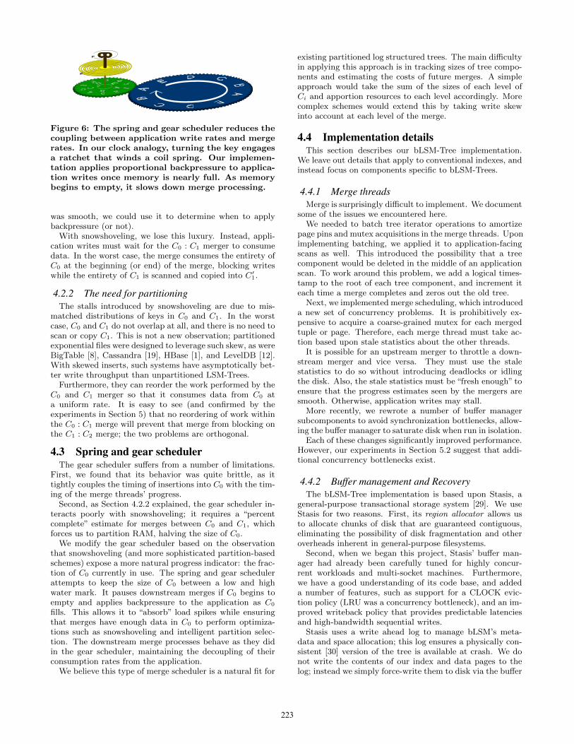
Downstream merges can take indefinitely long, and we areunwilling to give up write availability, so our only option isto synchronize merge completions with the processes that filleach tree component. Each process computes two progressindicators: inprogress and outprogress. In Figure 5, numbersrepresent the outprogress of C0 and the inprogress of C1. Let-ters represent the outprogress of C1 and the inprogress of C2.

We use a clock analogy to reason about the merge pro-cesses in our system. Clock gears ensure each hand movesat a consistent rate (so the minute and hour hand reach12 at the same time, for example). Our merge processesensure that trees fill at the same time as more space be-comes available downstream. As in a clock, multiple short

221

12

3 4

51

2

34

5543

2

1 A

BC

D E

AE

D C

BA

E

DC

B

Figure 5: The gear scheduler tracks the progress ofthe merges and ensures they complete at the sametime, preventing them from stalling the application.

upstream merges (sweeps of the minute hand) may occurper downstream merge (sweep of the hour hand). Unlikewith a clock, the only important synchronization point isthe hand-off from smaller component to larger (the meetingof the hands at 12).

We define inprogress as follows:

inprogressi =bytes read by mergei|C′i−1|+ |Ci|

Note that we ignore the cost of writing data to disk. An im-portant, but subtle property of inprogress is that any mergeactivity increases it, and that, within a single merge, thecost (in bytes transferred) of increasing inprogress by a fixedamount will never vary by more than a small constant factor.We say that estimators with this property are smooth.

Runs of deletions or non-overlapping ranges of the inputtrees can cause more intuitive estimates to become “stuck”at the same value for long periods of time. For example,early versions of our scheduler used estimates that focusedon I/O associated with the larger tree component (whichconsists of the bulk of the work). This led to routine stalls.

The definition of outprogress is more complex:

outprogressi =inprogressi + floor(|Ci|/|RAM |i)

ceil(R)

Returning to our clock analogy, the floor term is the com-putation one uses to determine what hour is being displayedby an analog clock.

Assuming an insert-only workload, each tree needs to bemerged R times before it fills up and becomes ready to bemerged with the downstream tree. The floor term usescurrent tree sizes to estimate the number of such merges this

tree component has undergone. |Ci||RAM|i must be less than

R, or the previous merge completion would have triggereda merge between Ci and Ci+1. This, combined with thefact that inprogressi ranges from zero to one ensures thatoutprogress ranges from zero to one, and that it is set to oneimmediately before a new merge is triggered. Finally, withina given merge with the upstream tree, outprogress inheritsits smoothness property from inprogress.

Across merges, workload shifts could cause the currenttree to shrink (for example, the application could deletedata), which could cause outprogress to decrease substan-tially. This will cause the downstream mergers to shut downuntil the current tree increases in size. If we had been ableto predict the workload shift ahead of time, we could havethrottled the application less aggressively. Since we cannot

predict future workload shifts, pausing downstream mergersseems to be the best approach.

Section 5.2 presents a timeseries plot of the write through-put of our index. The throughput varies by a bit under a fac-tor of two due to errors in our inprogress and outprogress esti-mates. In results not presented here, we experimented withbetter estimators of inprogress and outprogress but found thatexternal factors such as I/O interference lead to more vari-ance than inaccuracies in our model.

4.2 SnowshovelingIn this section, we describe snowshoveling, also called tour-

nament sort or replacement-selection sort, which significantlyimproves throughput for sequential and some skewed work-loads. For random workloads, snowshoveling increases theeffective size of C0 by a factor of four, doubling write through-put. For adversarial workloads, it increases the size by a fac-tor of two. In the best case, updates arrive in sorted order,and it streams them directly to disk.

Unfortunately, snowshoveling can block application writesfor arbitrary periods of time. At the end of this section, weexplain how partitioning can be used to“fix up”the problemssnowshoveling creates.

The basic idea stems from the sorting algorithms used bytape and punch card based database systems. It is impor-tant to minimize the number of runs performed by mergesort on such machines, as merging N runs requires N phys-ical drives or multiple passes. Naive implementations fillRAM, sort its contents, and write a RAM-sized run. Snow-shoveling fills RAM, writes back the lowest valued item, andthen reads a value from the input. It proceeds by writingout the lowest key that comes after the last value written.

If the data arrives in random order, this doubles the lengthof runs, since, on average, each item has a 50% chance ofcoming after the cursor. When the run starts, most incomingdata lands after the cursor; at the end, almost all landsbefore it. Alternatively, if the input is already sorted, allwrites arrive after the cursor, and snowshoveling produces arun containing the entire input. In the worst case, updatesare in reverse sorted order, and the run is the size of RAM.

4.2.1 Implications for LSM-Tree mergesSnowshoveling increases the amount of data that each C0 :

C1 merge consumes. Recall from Section 2.3 that LSM-Tree

write amplification is O(√|data||RAM| ); snowshoveling effectively

increases |RAM |. In addition to generating longer sortedruns, it eliminates the partitioning of C0 and C′0.

In the gear scheduler, each merge reads from a special treecomponent C′i−1 instead of directly from Ci−1. Incomingwrites are delivered to Ci−1, which atomically replaces C′i−1

when it is ready to be merged with the downstream tree.This is particularly inconvenient for C0, since it halves thepool of RAM that can be used for writes; after all, at theend of a C0 to C1 merge, the data stored in C′0 is uselessand discarded. Snowshoveling ensures that the entire poolcontains useful data at all times. This, combined with thefactor of two improvement it provides for random writes,is the basis of our claim that snowshoveling increases theeffective size of C0 by a factor of four.

However, breaking the partitioning between old and newupdates risks stalling application writes. Partitioning thewrite pool decoupled application writes from the rate atwhich data from C′0 is consumed. Thus, as long as inprogress

222

1 2 3 4 512

345 A

BC D E A E D C BAE

DCB

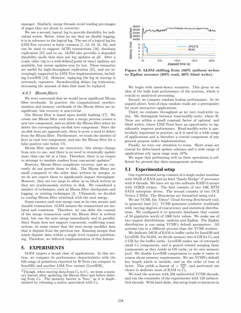
Figure 6: The spring and gear scheduler reduces thecoupling between application write rates and mergerates. In our clock analogy, turning the key engagesa ratchet that winds a coil spring. Our implemen-tation applies proportional backpressure to applica-tion writes once memory is nearly full. As memorybegins to empty, it slows down merge processing.

was smooth, we could use it to determine when to applybackpressure (or not).

With snowshoveling, we lose this luxury. Instead, appli-cation writes must wait for the C0 : C1 merger to consumedata. In the worst case, the merge consumes the entirety ofC0 at the beginning (or end) of the merge, blocking writeswhile the entirety of C1 is scanned and copied into C′1.

4.2.2 The need for partitioningThe stalls introduced by snowshoveling are due to mis-

matched distributions of keys in C0 and C1. In the worstcase, C0 and C1 do not overlap at all, and there is no need toscan or copy C1. This is not a new observation; partitionedexponential files were designed to leverage such skew, as wereBigTable [8], Cassandra [19], HBase [1], and LevelDB [12].With skewed inserts, such systems have asymptotically bet-ter write throughput than unpartitioned LSM-Trees.

Furthermore, they can reorder the work performed by theC0 and C1 merger so that it consumes data from C0 ata uniform rate. It is easy to see (and confirmed by theexperiments in Section 5) that no reordering of work withinthe C0 : C1 merge will prevent that merge from blocking onthe C1 : C2 merge; the two problems are orthogonal.

4.3 Spring and gear schedulerThe gear scheduler suffers from a number of limitations.

First, we found that its behavior was quite brittle, as ittightly couples the timing of insertions into C0 with the tim-ing of the merge threads’ progress.

Second, as Section 4.2.2 explained, the gear scheduler in-teracts poorly with snowshoveling; it requires a “percentcomplete” estimate for merges between C0 and C1, whichforces us to partition RAM, halving the size of C0.

We modify the gear scheduler based on the observationthat snowshoveling (and more sophisticated partition-basedschemes) expose a more natural progress indicator: the frac-tion of C0 currently in use. The spring and gear schedulerattempts to keep the size of C0 between a low and highwater mark. It pauses downstream merges if C0 begins toempty and applies backpressure to the application as C0

fills. This allows it to “absorb” load spikes while ensuringthat merges have enough data in C0 to perform optimiza-tions such as snowshoveling and intelligent partition selec-tion. The downstream merge processes behave as they didin the gear scheduler, maintaining the decoupling of theirconsumption rates from the application.

We believe this type of merge scheduler is a natural fit for

existing partitioned log structured trees. The main difficultyin applying this approach is in tracking sizes of tree compo-nents and estimating the costs of future merges. A simpleapproach would take the sum of the sizes of each level ofCi and apportion resources to each level accordingly. Morecomplex schemes would extend this by taking write skewinto account at each level of the merge.

4.4 Implementation detailsThis section describes our bLSM-Tree implementation.

We leave out details that apply to conventional indexes, andinstead focus on components specific to bLSM-Trees.

4.4.1 Merge threadsMerge is surprisingly difficult to implement. We document

some of the issues we encountered here.We needed to batch tree iterator operations to amortize

page pins and mutex acquisitions in the merge threads. Uponimplementing batching, we applied it to application-facingscans as well. This introduced the possibility that a treecomponent would be deleted in the middle of an applicationscan. To work around this problem, we add a logical times-tamp to the root of each tree component, and increment iteach time a merge completes and zeros out the old tree.

Next, we implemented merge scheduling, which introduceda new set of concurrency problems. It is prohibitively ex-pensive to acquire a coarse-grained mutex for each mergedtuple or page. Therefore, each merge thread must take ac-tion based upon stale statistics about the other threads.

It is possible for an upstream merger to throttle a down-stream merger and vice versa. They must use the stalestatistics to do so without introducing deadlocks or idlingthe disk. Also, the stale statistics must be “fresh enough” toensure that the progress estimates seen by the mergers aresmooth. Otherwise, application writes may stall.

More recently, we rewrote a number of buffer managersubcomponents to avoid synchronization bottlenecks, allow-ing the buffer manager to saturate disk when run in isolation.

Each of these changes significantly improved performance.However, our experiments in Section 5.2 suggest that addi-tional concurrency bottlenecks exist.

4.4.2 Buffer management and RecoveryThe bLSM-Tree implementation is based upon Stasis, a

general-purpose transactional storage system [29]. We useStasis for two reasons. First, its region allocator allows usto allocate chunks of disk that are guaranteed contiguous,eliminating the possibility of disk fragmentation and otheroverheads inherent in general-purpose filesystems.

Second, when we began this project, Stasis’ buffer man-ager had already been carefully tuned for highly concur-rent workloads and multi-socket machines. Furthermore,we have a good understanding of its code base, and addeda number of features, such as support for a CLOCK evic-tion policy (LRU was a concurrency bottleneck), and an im-proved writeback policy that provides predictable latenciesand high-bandwidth sequential writes.

Stasis uses a write ahead log to manage bLSM’s meta-data and space allocation; this log ensures a physically con-sistent [30] version of the tree is available at crash. We donot write the contents of our index and data pages to thelog; instead we simply force-write them to disk via the buffer

223

manager. Similarly, merge threads avoid reading pre-imagesof pages they are about to overwrite.

We use a second, logical, log to provide durability for indi-vidual writes. Below, when we say that we disable logging,it is in reference to the logical log. The use of a logical log forLSM-Tree recovery is fairly common [1, 12, 19, 31, 34], andcan be used to support ACID transactions [16], databasereplication [31] and so on. bLSM also provides a degradeddurability mode that does not log updates at all. After acrash, older (up to a well-defined point in time) updates areavailable, but recent updates may be lost. These semanticsare useful for high-throughput replication [31], and are in-creasingly supported by LSM-Tree implementations, includ-ing LevelDB [12]. However, replaying the log at startup isextremely expensive. Snowshoveling delays log truncation,increasing the amount of data that must be replayed.

4.4.3 Bloom filtersWe were concerned that we would incur significant Bloom

filter overheads. In practice, the computational, synchro-nization and memory overheads of the Bloom filters are in-significant, but recovery is non-trivial.

Our Bloom filter is based upon double hashing [17]. Wecreate one Bloom filter each time a merge process creates anew tree component, and we delete the Bloom filter when wedelete the corresponding on-disk tree component. Since theon-disk trees are append-only, there is never a need to deletefrom the Bloom filter. Furthermore, we track the number ofkeys in each tree component, and size the Bloom filter for afalse positive rate below 1%.

Bloom filter updates are monotonic; bits always changefrom zero to one, and there is no need to atomically updatemore than one bit at a time. Therefore, there is no reasonto attempt to insulate readers from concurrent updates.2

However, Bloom filters complicate recovery, and we cur-rently do not persist them to disk. The Bloom filters aresmall compared to the other data written by merges, sowe do not expect them to significantly impact throughput.However, they are too large to allow us to block writers asthey are synchronously written to disk. We considered anumber of techniques, such as Bloom filter checkpoints andlogging, or existing techniques [4]. Ultimately, we decidedto overlap Bloom filter writeback with the next merge.

Stasis ensures each tree merge runs in its own atomic anddurable transaction. bLSM ensures the transactions are iso-lated and consistent. Therefore, we can defer the commitof the merge transaction until the Bloom filter is writtenback, but run the next merge immediately and in parallel.Since Stasis does not support concurrent, conflicting trans-actions, we must ensure that the next merge modifies datathat is disjoint from the previous one. Running merges thattouch disjoint data within a single level requires partition-ing. Therefore, we deferred implementation of this feature.

5. EXPERIMENTSbLSM targets a broad class of applications. In this sec-

tion, we compare its performance characteristics with thefull range of primitives exported by B-Trees (we compare toInnoDB) and another LSM-Tree variant (LevelDB).

2Though, when moving data from C0 to C1, we issue a mem-ory barrier after updating the Bloom filter and before delet-ing from C0. The memory barrier is “free,” as it is imple-mented by releasing a mutex associated with C0.

ops/

sec

4400048000520005600060000

elapsed time (s)10 510 1010 1510 2010

late

ncy

(ms)

02468

UPDATEREAD

Figure 9: bLSM shifting from 100% uniform writesto Zipfian accesses (80% read, 20% blind write).

We begin with insert-heavy scenarios. This gives us anidea of the bulk load performance of the systems, which iscrucial to analytical processing.

Second, we compare random lookup performance. As weargued above, best-of-class random reads are a prerequisitefor most interactive applications.

Third, we evaluate throughput as we vary read:write ra-tios. We distinguish between read-modify-write, where B-Trees are within a small constant factor of optimal, andblind writes, where LSM-Trees have an opportunity to sig-nificantly improve performance. Read-modify-write is par-ticularly important in practice, as it is used by a wide rangeof applications and is therefore a crucial component of anygeneral purpose index implementation.

Finally, we turn our attention to scans. Short scans arecrucial for delta-based update schemes and a wide range ofapplications rely upon range scan APIs.

We argue that performing well on these operations is suf-ficient for present-day data management systems.

5.1 Experimental setupOur experimental setup consists of a single socket machine

with 16GB of RAM and an Intel “Sandy Bridge” i7 processorwith 8 threads. We have set up two software RAID 0 arrayswith 512KB stripes. The first consists of two 10K RPMSATA enterprise drives. The second consists of two OCZVertex 2 SSDs. The filesystems are formatted using ext4.

We use YCSB, the Yahoo! Cloud Serving Benchmark tool,to generate load [11]. YCSB generates synthetic workloadswith varying degrees of concurrency and statistical distribu-tions. We configured it to generate databases that consistof 50 gigabytes worth of 1000 byte values. We make use oftwo request distributions: uniform and Zipfian. The Zipfiandistribution is run using YCSB’s default parameters. Allsystems run in a different process than the YCSB workers.

We dedicate 10GB of RAM to buffer cache for InnoDB andLevelDB. For bLSM, we divide memory into 8 GB for C0 and2 GB for the buffer cache. LevelDB makes use of extremelysmall C0 components, and is geared toward merging thesecomponents as they reside in OS cache, or its own memorypool. We disable LevelDB compression to make it easier toreason about memory requirements. We use YCSB’s defaultkey length which is variable, and on the order of tens ofbytes. This yields a fanout of > 4096

50, and motivated our

choice to dedicate most of RAM to C0.We load the systems with 256 unthrottled YCSB threads,

and run the remainder of the experiments with 128 unthrot-tled threads. With hard disks, this setup leads to latencies in

224

ops/

sec

500015000250003500045000

elapsed time (s)10 510 1010 1510 2010 2510

late

ncy

(ms)

010203040

INSERT

ops/

sec

010000200003000040000500006000070000

elapsed time (s)10 2010 4010 6010 8010 10010

late

ncy

(ms)

02000400060008000

1000012000

INSERT

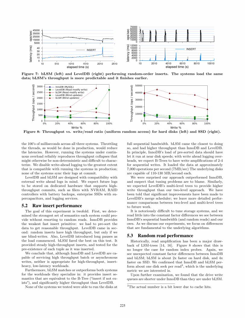
Figure 7: bLSM (left) and LevelDB (right) performing random-order inserts. The systems load the samedata; bLSM’s throughput is more predictable and it finishes earlier.

0% 20% 40% 60% 80% 100%

Write %

0

500

1000

1500

2000

2500

3000

Thro

ughput

(ops

/ se

cond)

InnoDB (MySQL)LevelDB (Read modify write)bLSM (Read modify write)LevelDB (Blind updates)bLSM (Blind updates)

0% 20% 40% 60% 80% 100%

Write %

0

10000

20000

30000

40000

50000

Thro

ughput

(ops

/ se

cond)

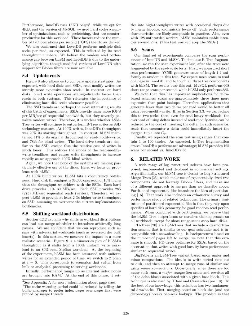
Figure 8: Throughput vs. write/read ratio (uniform random access) for hard disks (left) and SSD (right).

the 100’s of milliseconds across all three systems. Throttlingthe threads, as would be done in production, would reducethe latencies. However, running the systems under contin-uous overload reliably reproduces throughput collapses thatmight otherwise be non-deterministic and difficult to charac-terize. We disable write-ahead logging to the greatest extentthat is compatible with running the systems in production;none of the systems sync their logs at commit.

LevelDB and bLSM are designed with compatibility withexternal write ahead logs in mind. We expect future logsto be stored on dedicated hardware that supports high-throughput commits, such as filers with NVRAM, RAIDcontrollers with battery backups, enterprise SSDs with su-percapacitors, and logging services.

5.2 Raw insert performanceThe goal of this experiment is twofold. First, we deter-

mined the strongest set of semantics each system could pro-vide without resorting to random reads. InnoDB providesthe weakest fast insert primitive: we had to pre-sort thedata to get reasonable throughput. LevelDB came in sec-ond: random inserts have high throughput, but only if weuse blind-writes. Also, LevelDB introduced long pauses asthe load commenced. bLSM fared the best on this test. Itprovided steady high-throughput inserts, and tested for thepre-existence of each tuple as it was inserted.

We conclude that, although InnoDB and LevelDB are ca-pable of servicing high throughput batch or asynchronouswrites, neither is appropriate for high-throughput, insert-heavy, low-latency workloads.

Furthermore, bLSM matches or outperforms both systemsfor the workloads they specialize in: it provides insert se-mantics that are equivalent to the B-Tree (“insert if not ex-ists”), and significantly higher throughput than LevelDB.

None of the systems we tested were able to run the disks at

full sequential bandwidth. bLSM came the closest to doingso, and had higher throughput than InnoDB and LevelDB.In principle, InnoDB’s load of pre-sorted data should havelet it run at near disk speeds; with write ahead logging over-heads, we expect B-Trees to have write amplifications of 2-4for sequential writes. It loaded the data at approximately7,000 operations per second (7MB/sec) The underlying disksare capable of 110-130 MB/second each.

We were surprised our approach outperformed InnoDB,and suspect that tuning problems are to blame. Similarly,we expected LevelDB’s multi-level trees to provide higherwrite throughput than our two-level approach. We havebeen told that significant improvements have been made toLevelDB’s merge scheduler; we leave more detailed perfor-mance comparisons between two-level and multi-level treesto future work.

It is notoriously difficult to tune storage systems, and weread little into the constant factor differences we see betweenInnoDB’s sequential bandwidth (and random reads) and ourown. As we discuss our experiments, we focus on differencesthat are fundamental to the underlying algorithms.

5.3 Random read performanceHistorically, read amplification has been a major draw-

back of LSM-trees [14, 16]. Figure 8 shows that this isno longer the case for random index probes. Again, wesee unexpected constant factor differences between InnoDBand bLSM; bLSM is about 2x faster on hard disk, and 4xfaster on SSD. We confirmed that InnoDB and bLSM per-form about one disk seek per read3, which is the underlyingmetric we are interested in.

Upon further examination, we found that the drive writequeues are shorter under InnoDB than they are under bLSM.

3The actual number is a bit lower due to cache hits.

225

Furthermore, InnoDB uses 16KB pages4, while we opt for4KB, and the version of MySQL we used hard codes a num-ber of optimizations, such as prefetching, that are counter-productive for this workload. These factors reduce the num-ber of I/O operations per second (IOPS) the drives deliver.

We also confirmed that LevelDB performs multiple diskseeks per read, as expected. This is reflected by its readthroughput numbers. We believe the random read perfor-mance gap between bLSM and LevelDB is due to the under-lying algorithm, though modified versions of LevelDB withsupport for Bloom filters are now available.

5.4 Update costsFigure 8 also allows us to compare update strategies. As

expected, with hard disks and SSDs, read-modify-writes arestrictly more expensive than reads. In contrast, on harddisks, blind write operations are significantly faster thanreads in both systems. This reiterates the importance ofeliminating hard disk seeks whenever possible.

The SSD trends are perhaps the most interesting resultsof this batch of experiments. SSDs provide many more IOPSper MB/sec of sequential bandwidth, but they severely pe-nalize random writes. Therefore, it is unclear whether LSM-Tree writes will continue to outperform B-Tree writes as SSDtechnology matures. At 100% writes, InnoDB’s throughputwas 20% its starting throughput. In contrast, bLSM main-tained 41% of its original throughput for read-modify-write,and 78% for blind writes. The hard drive trends are sim-ilar to the SSD, except that the relative cost of writes ismuch lower. This reduces the slopes of the read-modify-write trendlines, and causes write throughputs to increaserapidly as we approach 100% blind writes.

Again, we note that none of the systems are making par-ticularly effective use of the disks. Here, we focus on prob-lems with bLSM.

At 100% blind writes, bLSM hits a concurrency bottle-neck. Hard disk throughput is 33,000 ops/second; 10% higherthan the throughput we achieve with the SSDs. Each harddrive provides 110-130 MB/sec. Each SSD provides 285(275) MB/sec sequential reads (writes). Therefore, we ex-pect bLSM to provide at least 2-3x higher write throughputon SSD, assuming we overcome the current implementationbottlenecks.

5.5 Shifting workload distributionsSection 4.2.2 explains why shifts in workload distributions

can lead our merge scheduler to introduce arbitrarily longpauses. We are confident that we can reproduce such is-sues with adversarial workloads (such as reverse-order bulkinserts). In this section, we measure the impact in a morerealistic scenario. Figure 9 is a timeseries plot of bLSM’sthroughput as it shifts from a 100% uniform write work-load to an 80% read Zipfian workload. At the beginningof the experiment, bLSM has been saturated with uniformwrites for an extended period of time; we switch to Zipfianat t = 0. This corresponds to scenarios that switch frombulk or analytical processing to serving workloads.

Initially, performance ramps up as internal index nodesare brought into RAM.5 At the end of this phase, it set-

4See Appendix A for more information about page sizes.5The cache warming period could be reduced by telling thebuffer manager to prefer index pages over pages that werepinned by merge threads.

tles into high-throughput writes with occasional drops dueto merge hiccups, and quickly levels off. Such performancecharacteristics are likely acceptable in practice. Also, evenwith 128 unthrottled workers, bLSM maintains stable laten-cies around 2ms. (This test was run atop the SSDs.)

5.6 ScansOur final set of experiments compares the scan perfor-

mance of InnoDB and bLSM. To simulate B-Tree fragmen-tation, we ran the scan experiment last, after the trees werefragmented by the read-write tests. First, we measured shortscan performance. YCSB generates scans of length 1-4 uni-formly at random in this test. We expect most scans to readone page in InnoDB, and to touch all three tree componentswith bLSM. The results bear this out. MySQL performs 608short range scans per second, while bLSM only performs 385.

We note that this has important implications for delta-based schemes: scans are approximately three times moreexpensive than point lookups. Therefore, applications thatgenerate fewer than two deltas per read would be better offusing read-modify-write. If, as in Section 3.3, we can reducethis to two seeks, then, even for read heavy workloads, theoverhead of using deltas instead of read-modify-write can bereduced to the cost of inserting the delta. In such scenarios,reads that encounter a delta could immediately insert themerged tuple into C0.

Finally, we repeated the scan test using ranges that con-tain 1 to 100 tuples. As expected, B-Tree fragmentationerases InnoDB’s performance advantage; bLSM provides 165scans per second vs. InnoDB’s 86.

6. RELATED WORKA wide range of log structured indexes have been pro-

posed, implemented and deployed in commercial settings.Algorithmically, our bLSM-tree is closest to Log StructuredMerge Trees [25], which make use of exponentially sized treecomponents, do not leverage Bloom filters, and make useof a different approach to merges than we describe above.Partitioned exponential files introduce the idea of partition-ing [16]. That work also includes an exhaustive survey andperformance study of related techniques. The primary limi-tation of partitioned exponential files is that they rely uponspecifics of hard disk geometry for good random read perfor-mance. When combined with partitioning, we believe thatthe bLSM-Tree outperforms or matches their approach onall workloads except for short range scans atop hard disks.

FD-Trees [20] are LSM-Trees that include a deamortiza-tion scheme that is similar to our gear scheduler and is in-compatible with snowshoveling. It backpressures based onthe number of pages left to merge; we note that this esti-mate is smooth. FD-Trees optimize for SSDs, based on theobservation that writes with good locality have performancesimilar to sequential writes.

BigTable is an LSM-Tree variant based upon major andminor compactions. The idea is to write sorted runs outto disk, and then to attempt to merge runs of similar sizeusing minor compactions. Occasionally, when there are toomany such runs, a major compaction scans and rewrites allof the delta blocks associated with a given base block. Thistechnique is also used by HBase and Cassandra (pre 1.0). Tothe best of our knowledge, this technique has two fundamen-tal drawbacks. First, merging based on block size (and notchronology) breaks one-seek lookups. The problem is that

226

some unsearched block could have a newer delta, so extrabase records and deltas must be fetched from disk. Fur-thermore, without a more specific merge policy, it is verydifficult to reason about the amortized cost of inserts. Tothe best of our knowledge, all current implementations ofthis approach suffer from write pauses or degraded reads.

Cassandra version 1.0 adds a merger based upon exponen-tial sizing and addresses the problem of write pauses [13].If merges fall behind it writes additional (perhaps overlap-ping) range partitions to C1, degrading scans but allowingwrites to continue to be serviced.

TokuDB [18] and LevelDB [12] both make use of parti-tioned, exponentially sized levels and fractional cascading.As we argued above, this improves write throughput at theexpense of reads and scans. Riak modified LevelDB to sup-port Bloom filters and improved the merge scheduler [3].These structures are related to cache oblivious lookup arrays(COLA) and streaming B-trees [5], which include deamorti-zation algorithms with goals similar to our merge schedulers,except that they introduce extra work to each operation,while we focus on rate-limiting asynchronous backgroundprocesses to keep the system in a favorable steady state.

The bLSM implementation is based upon Rose, a column-compressed LSM-Tree for database replication tasks [31].Rose does not employ Bloom filters and has a naive mergescheduler with unbounded write latency. The compressiontechniques lead to constant factor decreases in write ampli-fication and do not impact reads. LevelDB makes use of ageneral-purpose compression algorithm.

A number of flash-optimized indexes have been proposedfor use in embedded systems, including FlashDB [24], whichvaries its layout based upon read-write ratios and hardwareparameters (as do TokuDB and many major-minor com-paction systems), and MicroHash [35], which targets embed-ded devices and has extremely high read fanout. In contrastto these systems, we achieve lower read and write amplifica-tions, but assume ample main memory is available.

We do not have space to cover unordered approaches insufficient detail; the LFS (Log File System) introduced manyof the techniques used by such systems. WAFL [27] is acommercially-available hybrid filesystem that stores smallobjects in an LFS-like format. BitCask [33], BDB-JE [26]and Primebase [2] are contemporary examples in the keyvalue and database space. BDB-JE uses unordered storagefor data, but a B-Tree for the index, allowing it to perform(potentially seek-intensive) scans. Primebase is a log struc-tured MySQL storage engine. SILT is an unordered storethat uses 0.7 bytes per key to achieve a read amplificationof 1 [21].

A number of indexes target hybrid storage systems. LHAMindexes provide historical queries over write-once-read-many(WORM) storage [23], and multi-tier GTSSL log structuredindexes target hybrid disk-flash systems and adapt to vary-ing read-write ratios [34].

7. CONCLUSIONbLSM-Trees provide a superset of standard B-Tree func-

tionality; they introduce a zero-seek “blind write” primi-tive. Blind writes enable high-throughput writes and insertsagainst existing data structures, which are crucial for ana-lytical processing and emerging classes of applications.

Our experiments show that, with the exception of shortrange scans (a primitive which is primarily useful for leverag-

ing blind writes), bLSM-Trees provide superior performanceacross the entire B-Tree API. These results rely heavily uponour use of a three-level bLSM-tree and Bloom filters.

However, our spring and gear scheduler is what ultimatelyallows bLSM-Trees to act as drop-in B-Tree replacements.Eliminating write throughput collapses greatly simplifies op-erations tasks and allows bLSM-Trees to be deployed as theprimary backing store for interactive workloads.

These results come with two caveats. First, the rela-tive performance of update-in-place and log-structured ap-proaches is subject to changes in the underlying devices.Second, we target applications that manage small pieces ofdata. Fundamentally, log structured approaches work byreplacing random I/O with sequential I/O. As the size ofobjects increase, the sequential costs dominate and update-in-place techniques provide superior performance.

Furthermore, a number of technical issues remain. Oursystem remains a partial solution; it cannot yet leverage(or gracefully cope with) write skew. Also, transitioning tological logging has wide ranging impacts on recovery, lockmanagement, and other higher-level database mechanisms.

Well-known techniques address each of these remainingconcerns; we look forward to applying these techniques tobuild unified transaction and analytical processing systems.

8. ACKNOWLEDGMENTSWe would like to thank Mark Callaghan, Brian Cooper,

the members of the PNUTS team, and our shepherd, RyanJohnson for their invaluable feedback.

bLSM is open source and available for download:

http://www.github.com/sears/bLSM/

9. REFERENCES[1] http://hbase.apache.org/.

[2] https://launchpad.net/pbxt.

[3] http://wiki.basho.com/.[4] M. Bender, M. Farach-Colton, R. Johnson, B. Kuszmaul,

D. Medjedovic, P. Montes, P. Shetty, R. Spillane, andE. Zadok. Don’t thrash: How to cache your hash on flash.In HotStorage, 2011.

[5] M. A. Bender, M. Farach-Colton, J. T. Fineman, Y. R.Fogel, B. C. Kuszmaul, and J. Nelson. Cache-obliviousstreaming B-trees. In SPAA, 2007.

[6] D. Borthakur, J. Gray, J. Sarma, K. Muthukkaruppan,N. Spiegelberg, H. Kuang, K. Ranganathan, D. Molkov,A. Menon, S. Rash, et al. Apache Hadoop goes realtime atFaceBook. In Sigmod, 2011.

[7] M. Callaghan. Read amplification factor. High AvailabilityMySQL, August 2011.

[8] F. Chang et al. Bigtable: A distributed storage system forstructured data. In OSDI, 2006.

[9] J. Chen, C. Douglas, M. Mutsuzaki, P. Quaid,R. Ramakrishnan, S. Rao, and R. Sears. Walnut: A unifiedcloud object store. In Sigmod, 2012.

[10] B. F. Cooper et al. PNUTS: Yahoo!’s hosted data servingplatform. Proc. VLDB Endow., 1(2), 2008.

[11] B. F. Cooper, A. Silberstein, E. Tam, R. Ramakrishnan,and R. Sears. Benchmarking cloud serving systems withYCSB. SoCC ’10, 2010.

[12] J. Dean and S. Ghemawat. LevelDB. Google,http://leveldb.googlecode.com.

[13] J. Ellis. The present and future of Apache Cassandra. InHPTS, 2011.

[14] S. Ghemawat, H. Gobioff, and S. T. Leung. The Google filesystem. In SOSP, 2003.

227

SSD Hard diskSATA PCI-E Server Media

Capacity (GB) 512 5000 300 2000Reads / second 50K 1M 500 250Access Frequency GB of B-Tree index cache per drive

Minute 0.302 6.03 0.003 0.002Five minute 1.51 30.2 0.015 0.008

Half hour 9.05 - 0.091 0.045Hour - - 0.181 0.091Day - - 4.35 2.17

Week - - - 15.2Month - - - -

Full disk 12.5 122 7.32 48.8

Table 2: RAM required to cache B-Tree nodes toaddress various storage devices. Hot data causesdevices to be seek bound, leading to unused capacityand less cache. We assume 100 byte keys, 1000 bytevalues and 4096 byte pages.

[15] J. Gray and G. Graefe. The five-minute rule ten years later,and other computer storage rules of thumb. SIGMODRecord, 26(4), 1997.

[16] C. Jermaine, E. Omiecinski, and W. G. Yee. Thepartitioned exponential file for database storagemanagement. The VLDB Journal, 16(4), 2007.

[17] Kirsch and Mitzenmacher. Less hashing, same performance:Building a better bloom filter. In ESA, 2006.

[18] B. C. Kuszmaul. How TokuDB fractal trees indexes work.Technical report, TokuTek, 2010.

[19] A. Lakshman and P. Malik. Cassandra: a decentralizedstructured storage system. SIGOPS Oper. Syst. Rev.,44(2), April 2010.

[20] Y. Li, B. He, J. Y. 0001, Q. Luo, and K. Yi. Tree indexingon solid state drives. PVLDB, 3(1):1195–1206, 2010.

[21] H. Lim, B. Fan, D. Andersen, and M. Kaminsky. Silt: amemory-efficient, high-performance key-value store. InSOSP, 2011.

[22] M. Moshayedi and P. Wilkison. Enterprise SSDs. ACMQueue, 6, July 2008.

[23] P. Muth, P. O’Neil, A. Pick, and G. Weikum. The LHAMLog-structured history data access method. In VLDBJournal, 2000.

[24] S. Nath and A. Kansal. FlashDB: Dynamic self-tuningdatabase for NAND flash. In IPSN, 2007.

[25] P. O’Neil, E. Cheng, D. Gawlick, and E. O’Neil. Thelog-structured merge-tree (LSM-tree). Acta Informatica,33(4):351–385, 1996.

[26] Oracle. Berkeley DB Java Edition.[27] C. Rev, D. Hitz, J. Lau, and M. Malcolm. File system

design for an NFS file server appliance, 1995.[28] M. Rosenblum and J. K. Ousterhout. The design and

implementation of a log-structured file system. In SOSP,1992.

[29] R. Sears and E. Brewer. Stasis: Flexible transactionalstorage. In OSDI, 2006.

[30] R. Sears and E. Brewer. Segment-based recovery:Write-ahead logging revisited. In VLDB, 2009.

[31] R. Sears, M. Callaghan, and E. Brewer. Rose: Compressed,log-structured replication. VLDB, 2008.

[32] M. Seltzer, K. A. Smith, H. Balakrishnan, J. Chang,S. McMains, and V. Padmanabhan. File system loggingversus clustering: A performance comparison. In UsenixAnnual Technical Conference, 1995.

[33] J. Sheehy and D. Smith. Bitcask, a log-structured hashtable for fast key/value data. Technical report, Basho, 2010.

[34] R. Spillane, P. Shetty, E. Zadok, S. Archak, and S. Dixit.

An efficient multi-tier tablet server storage architecture. InSoCC, 2011.

[35] D. Zeinalipour-Yazti, S. Lin, V. Kalogeraki, D. Gunopulos,and W. Najjar. MicroHash: An efficient index structure forfash-based sensor devices. In FAST, 2005.

APPENDIXA. PAGE SIZES ON MODERN HARDWARE

In this section we argue that modern database systemsmake use of excessively large page sizes. Most systems makeuse of a computation that balances the cost of reading a pageagainst the search progress made by each page traversal [15].

This approach is flawed for two reasons: (1) Index pagesgenerally fit in RAM and should be sized to reduce the size ofthe tree’s upper levels. This is a function of key size, not thehardware. (2) Systems (but not the original analysis [15])often conflate optimal index page sizes with optimal datapage sizes. This simplifies implementations, but can severelyimpact performance if it leads to oversized data pages.

A.1 Index nodes generally fit in RAMAssuming index nodes are large enough to hold many keys,

we can ignore the upper levels of the tree and space wasteddue to index page boundaries. Therefore, we can fit approxi-mately memory size

key size+pointer sizepointers to leaf pages in memory.

Each such pointer addresses approximately

max(page size, key size + value size)

bytes of data, giving us a read fanout of:

max(page size, key size + value size)

key size + pointer size≈ page size

key size

“Typical” keys are under 100 bytes, and we use 4KB pages.This yields a read fanout of 40. Prefix compression andincreased data page sizes significantly improve matters.

Table 2 applies these calculations to various hardware de-vices, and reports the amount of RAM needed for a readamplification of one. As data becomes hotter, the devices be-come seek-bound instead of capacity-bound. This decreasesmemory requirements until data becomes so hot that it ismore economical to store it in memory than on disk [15].

Our Bloom filters consume 1.25 bytes per key and storeentries for all keys, not just those in index nodes. Fourentries fit on a leaf, leading to a 4 ∗ 1.25 = 5% overhead.

A.2 Choosing page sizes when RAM is largeSince index nodes generally fit in RAM, we choose their

size independently of the underlying disk. Index pages 10xthe average size of keys ensure that upper levels of the treeuse a small (and ignorable) fraction of RAM.

Pages that store data are subject to different page sizetradeoffs than pages that store index nodes. bLSM uses asimple append-only data page format that efficiently storesrecords that span multiple pages and bounds the fraction ofspace wasted by inconveniently sized records.

We set these pages to 4KB, which is the minimum SSDtransfer size. This minimizes transfer times and also im-proves cache behavior for workloads with poor locality: Itreduces the number of cold records that are read and cachedalongside hot records, increasing the average heat of thepages cached in RAM.

228