Bond Price Volatility - 國立臺灣大學lyuu/finance1/2008/20080227.pdf · † For a bond with positive convexity, the price rises more ... † In the bond price formula, Xn i=1

Bond Price Volatility

c©2008 Prof. Yuh-Dauh Lyuu, National Taiwan University Page 71

“Well, Beethoven, what is this?”— Attributed to Prince Anton Esterhazy


Price Volatility

• Volatility measures how bond prices respond to interestrate changes.

• It is key to the risk management ofinterest-rate-sensitive securities.

• Assume level-coupon bonds throughout.


Price Volatility (concluded)

• What is the sensitivity of the percentage price change tochanges in interest rates?

• Define price volatility by

−∂P∂y

P.


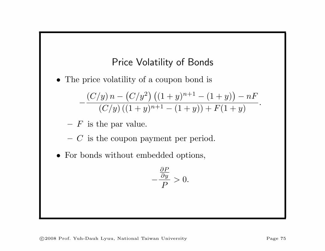
Price Volatility of Bonds

• The price volatility of a coupon bond is

− (C/y)n− (C/y2

) ((1 + y)n+1 − (1 + y)

)− nF

(C/y) ((1 + y)n+1 − (1 + y)) + F (1 + y).

– F is the par value.

– C is the coupon payment per period.

• For bonds without embedded options,

−∂P∂y

P> 0.


Macaulay Duration

• The Macaulay duration (MD) is a weighted average ofthe times to an asset’s cash flows.

• The weights are the cash flows’ PVs divided by theasset’s price.

• Formally,

MD ≡ 1P

n∑

i=1

iCi

(1 + y)i.

• The Macaulay duration, in periods, is equal to

MD = −(1 + y)∂P

∂y

1P

. (7)


MD of Bonds

• The MD of a coupon bond is

MD =1P

[n∑

i=1

iC

(1 + y)i+

nF

(1 + y)n

]. (8)

• It can be simplified to

MD =c(1 + y) [ (1 + y)n − 1 ] + ny(y − c)

cy [ (1 + y)n − 1 ] + y2,

where c is the period coupon rate.

• The MD of a zero-coupon bond equals its term tomaturity n.

• The MD of a coupon bond is less than its maturity.


Finesse

• Equations (7) on p. 76 and (8) on p. 77 hold only if thecoupon C, the par value F , and the maturity n are allindependent of the yield y.

– That is, if the cash flow is independent of yields.

• To see this point, suppose the market yield declines.

• The MD will be lengthened.

• But for securities whose maturity actually decreases as aresult, the MD (as originally defined) may actuallydecrease.


How Not To Think about MD

• The MD has its origin in measuring the length of time abond investment is outstanding.

• The MD should be seen mainly as measuring pricevolatility.

• Many, if not most, duration-related terminology cannotbe comprehended otherwise.


Conversion

• For the MD to be year-based, modify Eq. (8) on p. 77 to

1P

[n∑

i=1

i

k

C(1 + y

k

)i+

n

k

F(1 + y

k

)n

],

where y is the annual yield and k is the compoundingfrequency per annum.

• Equation (7) on p. 76 also becomes

MD = −(1 +

y

k

) ∂P

∂y

1P

.

• By definition, MD (in years) = MD (in periods)k .


Modified Duration

• Modified duration is defined as

modified duration ≡ −∂P

∂y

1P

=MD

(1 + y). (9)

• By Taylor expansion,

percent price change ≈ −modified duration× yield change.


Example

• Consider a bond whose modified duration is 11.54 with ayield of 10%.

• If the yield increases instantaneously from 10% to10.1%, the approximate percentage price change will be

−11.54× 0.001 = −0.01154 = −1.154%.


Modified Duration of a Portfolio

• The modified duration of a portfolio equals∑

i

ωiDi.

– Di is the modified duration of the ith asset.

– ωi is the market value of that asset expressed as apercentage of the market value of the portfolio.


Effective Duration

• Yield changes may alter the cash flow or the cash flowmay be so complex that simple formulas are unavailable.

• We need a general numerical formula for volatility.

• The effective duration is defined asP− − P+

P0(y+ − y−).

– P− is the price if the yield is decreased by ∆y.

– P+ is the price if the yield is increased by ∆y.

– P0 is the initial price, y is the initial yield.

– ∆y is small.

• See plot on p. 85.


y

P0

P+

P-

y+

y-


Effective Duration (concluded)

• One can compute the effective duration of just aboutany financial instrument.

• Duration of a security can be longer than its maturity ornegative!

• Neither makes sense under the maturity interpretation.

• An alternative is to use

P0 − P+

P0 ∆y.

– More economical but less accurate.


The Practices

• Duration is usually expressed in percentage terms—callit D%—for quick mental calculation.

• The percentage price change expressed in percentageterms is approximated by

−D% ×∆r

when the yield increases instantaneously by ∆r%.

– Price will drop by 20% if D% = 10 and ∆r = 2because 10× 2 = 20.

• In fact, D% equals modified duration as originallydefined (prove it!).


Hedging

• Hedging offsets the price fluctuations of the position tobe hedged by the hedging instrument in the oppositedirection, leaving the total wealth unchanged.

• Define dollar duration as

modified duration× price (% of par) = −∂P

∂y.

• The approximate dollar price change per $100 of parvalue is

price change ≈ −dollar duration× yield change.


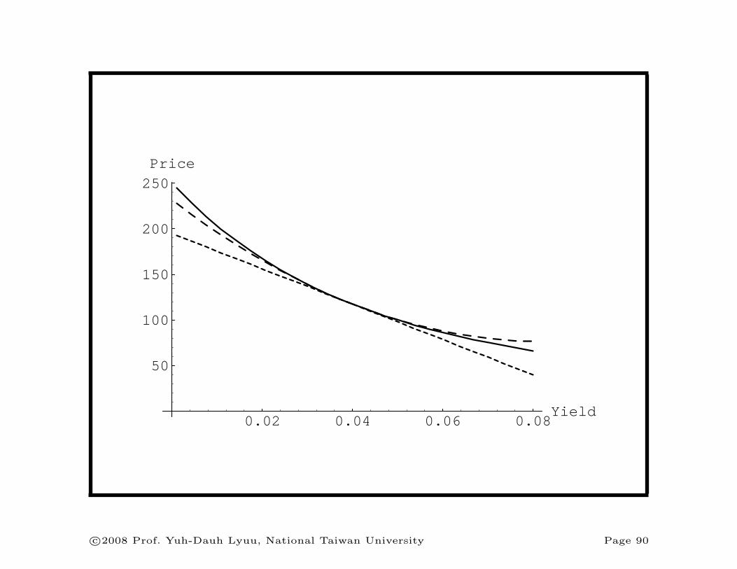
Convexity

• Convexity is defined as

convexity (in periods) ≡ ∂2P

∂y2

1P

.

• The convexity of a coupon bond is positive (prove it!).

• For a bond with positive convexity, the price rises morefor a rate decline than it falls for a rate increase of equalmagnitude (see plot next page).

• Hence, between two bonds with the same duration, theone with a higher convexity is more valuable.


0.02 0.04 0.06 0.08Yield

50

100

150

200

250

Price


Convexity (concluded)

• Convexity measured in periods and convexity measuredin years are related by

convexity (in years) =convexity (in periods)

k2

when there are k periods per annum.


Use of Convexity

• The approximation ∆P/P ≈ − duration× yield change

works for small yield changes.

• To improve upon it for larger yield changes, use

∆P

P≈ ∂P

∂y

1P

∆y +12

∂2P

∂y2

1P

(∆y)2

= −duration×∆y +12× convexity× (∆y)2.

• Recall the figure on p. 90.


The Practices

• Convexity is usually expressed in percentage terms—callit C%—for quick mental calculation.

• The percentage price change expressed in percentageterms is approximated by −D% ×∆r + C% × (∆r)2/2when the yield increases instantaneously by ∆r%.

– Price will drop by 17% if D% = 10, C% = 1.5, and∆r = 2 because

−10× 2 +12× 1.5× 22 = −17.

• In fact, C% equals convexity divided by 100 (prove it!).


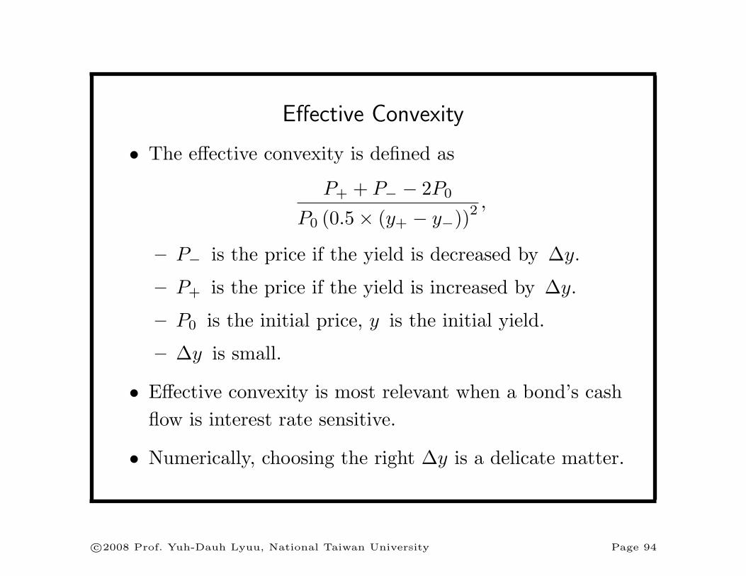
Effective Convexity

• The effective convexity is defined as

P+ + P− − 2P0

P0 (0.5× (y+ − y−))2,

– P− is the price if the yield is decreased by ∆y.

– P+ is the price if the yield is increased by ∆y.

– P0 is the initial price, y is the initial yield.

– ∆y is small.

• Effective convexity is most relevant when a bond’s cashflow is interest rate sensitive.

• Numerically, choosing the right ∆y is a delicate matter.


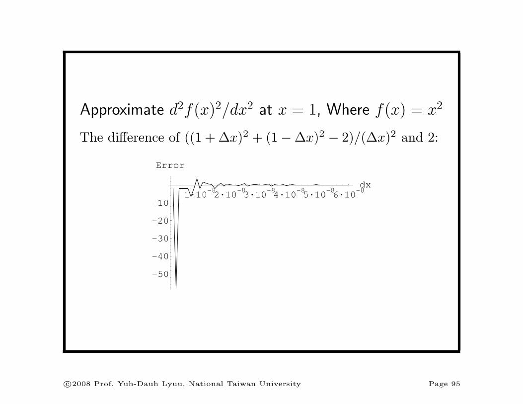
Approximate d2f(x)2/dx2 at x = 1, Where f(x) = x2

The difference of ((1 + ∆x)2 + (1−∆x)2 − 2)/(∆x)2 and 2:

1·10-82·10-83·10-84·10-85·10-86·10-8dx

-50

-40

-30

-20

-10

Error


Term Structure of Interest Rates


Why is it that the interest of money is lower,when money is plentiful?

— Samuel Johnson (1709–1784)

If you have money, don’t lend it at interest.Rather, give [it] to someone

from whom you won’t get it back.— Thomas Gospel 95


Term Structure of Interest Rates

• Concerned with how interest rates change with maturity.

• The set of yields to maturity for bonds forms the termstructure.

– The bonds must be of equal quality.

– They differ solely in their terms to maturity.

• The term structure is fundamental to the valuation offixed-income securities.


0 5 10 15 20 25 30Year

1234567

Yield (%)


Term Structure of Interest Rates (concluded)

• Term structure often refers exclusively to the yields ofzero-coupon bonds.

• A yield curve plots yields to maturity against maturity.

• A par yield curve is constructed from bonds tradingnear par.


Four Typical Shapes

• A normal yield curve is upward sloping.

• An inverted yield curve is downward sloping.

• A flat yield curve is flat.

• A humped yield curve is upward sloping at first but thenturns downward sloping.


Spot Rates

• The i-period spot rate S(i) is the yield to maturity ofan i-period zero-coupon bond.

• The PV of one dollar i periods from now is

[ 1 + S(i) ]−i.

• The one-period spot rate is called the short rate.

• Spot rate curve: Plot of spot rates against maturity.


Problems with the PV Formula

• In the bond price formula,n∑

i=1

C

(1 + y)i+

F

(1 + y)n,

every cash flow is discounted at the same yield y.

• Consider two riskless bonds with different yields tomaturity because of their different cash flow streams:

n1∑

i=1

C

(1 + y1)i+

F

(1 + y1)n1,

n2∑

i=1

C

(1 + y2)i+

F

(1 + y2)n2.


Problems with the PV Formula (concluded)

• The yield-to-maturity methodology discounts theircontemporaneous cash flows with different rates.

• But shouldn’t they be discounted at the same rate?


Spot Rate Discount Methodology

• A cash flow C1, C2, . . . , Cn is equivalent to a package ofzero-coupon bonds with the ith bond paying Ci dollarsat time i.

• So a level-coupon bond has the price

P =n∑

i=1

C

[ 1 + S(i) ]i+

F

[ 1 + S(n) ]n. (10)

• This pricing method incorporates information from theterm structure.

• Discount each cash flow at the corresponding spot rate.


Discount Factors

• In general, any riskless security having a cash flowC1, C2, . . . , Cn should have a market price of

P =n∑

i=1

Cid(i).

– Above, d(i) ≡ [ 1 + S(i) ]−i, i = 1, 2, . . . , n, are calleddiscount factors.

– d(i) is the PV of one dollar i periods from now.

• The discount factors are often interpolated to form acontinuous function called the discount function.


Extracting Spot Rates from Yield Curve

• Start with the short rate S(1).

– Note that short-term Treasuries are zero-couponbonds.

• Compute S(2) from the two-period coupon bond priceP by solving

P =C

1 + S(1)+

C + 100[ 1 + S(2) ]2

.


Extracting Spot Rates from Yield Curve (concluded)

• Inductively, we are given the market price P of then-period coupon bond and S(1), S(2), . . . , S(n− 1).

• Then S(n) can be computed from Eq. (10) on p. 105,repeated below,

P =n∑

i=1

C

[ 1 + S(i) ]i+

F

[ 1 + S(n) ]n.

• The running time is O(n) (see text).

• The procedure is called bootstrapping.


Some Problems

• Treasuries of the same maturity might be selling atdifferent yields (the multiple cash flow problem).

• Some maturities might be missing from the data points(the incompleteness problem).

• Treasuries might not be of the same quality.

• Interpolation and fitting techniques are needed inpractice to create a smooth spot rate curve.

– Any economic justifications?


Yield Spread

• Consider a risky bond with the cash flowC1, C2, . . . , Cn and selling for P .

• Were this bond riskless, it would fetch

P ∗ =n∑

t=1

Ct

[ 1 + S(t) ]t.

• Since riskiness must be compensated, P < P ∗.

• Yield spread is the difference between the IRR of therisky bond and that of a riskless bond with comparablematurity.


Static Spread

• The static spread is the amount s by which the spotrate curve has to shift in parallel to price the risky bond:

P =n∑

t=1

Ct

[ 1 + s + S(t) ]t.

• Unlike the yield spread, the static spread incorporatesinformation from the term structure.


Of Spot Rate Curve and Yield Curve

• yk: yield to maturity for the k-period coupon bond.

• S(k) ≥ yk if y1 < y2 < · · · (yield curve is normal).

• S(k) ≤ yk if y1 > y2 > · · · (yield curve is inverted).

• S(k) ≥ yk if S(1) < S(2) < · · · (spot rate curve isnormal).

• S(k) ≤ yk if S(1) > S(2) > · · · (spot rate curve isinverted).

• If the yield curve is flat, the spot rate curve coincideswith the yield curve.


Shapes

• The spot rate curve often has the same shape as theyield curve.

– If the spot rate curve is inverted (normal, resp.), thenthe yield curve is inverted (normal, resp.).

• But this is only a trend not a mathematical truth.a

aSee a counterexample in the text.


Forward Rates

• The yield curve contains information regarding futureinterest rates currently “expected” by the market.

• Invest $1 for j periods to end up with [ 1 + S(j) ]j

dollars at time j.

– The maturity strategy.

• Invest $1 in bonds for i periods and at time i invest theproceeds in bonds for another j − i periods where j > i.

• Will have [ 1 + S(i) ]i[ 1 + S(i, j) ]j−i dollars at time j.

– S(i, j): (j − i)-period spot rate i periods from now.

– The rollover strategy.


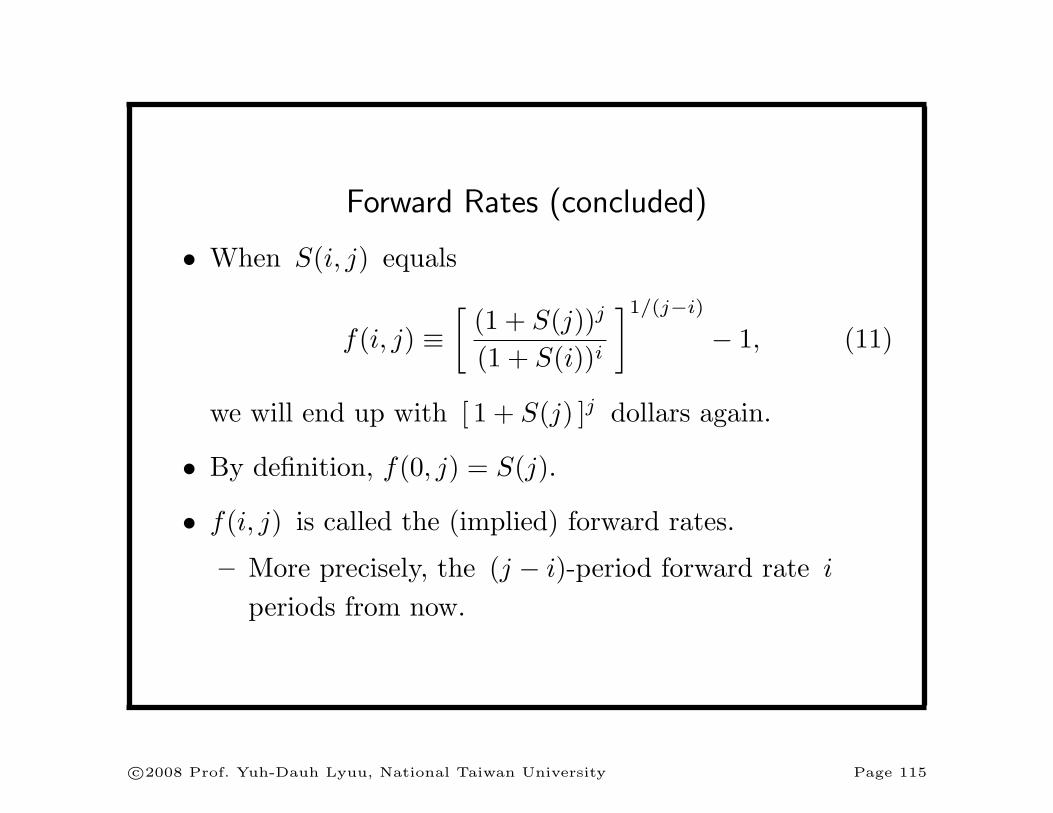
Forward Rates (concluded)

• When S(i, j) equals

f(i, j) ≡[

(1 + S(j))j

(1 + S(i))i

]1/(j−i)

− 1, (11)

we will end up with [ 1 + S(j) ]j dollars again.

• By definition, f(0, j) = S(j).

• f(i, j) is called the (implied) forward rates.

– More precisely, the (j − i)-period forward rate i

periods from now.


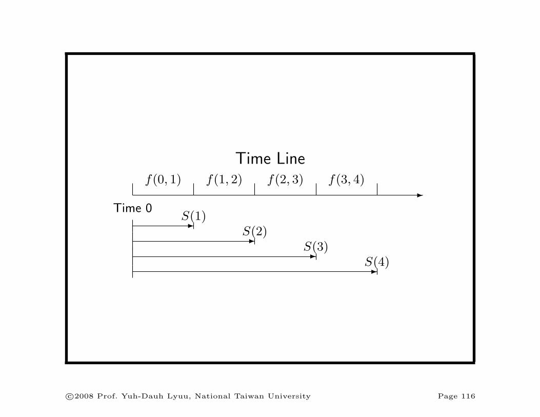
Time Line

-f(0, 1) f(1, 2) f(2, 3) f(3, 4)

Time 0-S(1)

-S(2)

-S(3)

-S(4)


Forward Rates and Future Spot Rates

• We did not assume any a priori relation between f(i, j)and future spot rate S(i, j).

– This is the subject of the term structure theories.

• We merely looked for the future spot rate that, ifrealized, will equate two investment strategies.

• f(i, i + 1) are instantaneous forward rates or one-periodforward rates.


Spot Rates and Forward Rates

• When the spot rate curve is normal, the forward ratedominates the spot rates,

f(i, j) > S(j) > · · · > S(i).

• When the spot rate curve is inverted, the forward rate isdominated by the spot rates,

f(i, j) < S(j) < · · · < S(i).


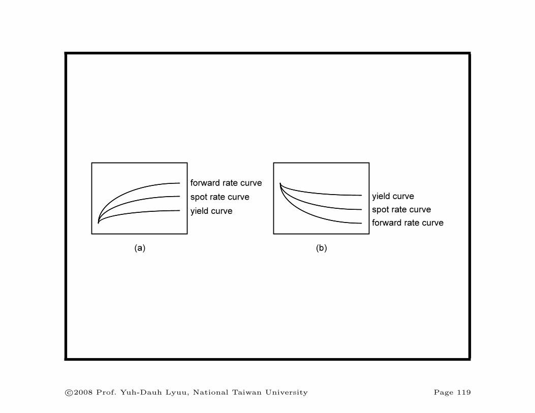
spot rate curve

forward rate curve

yield curve

(a)

spot rate curve

forward rate curve

yield curve

(b)


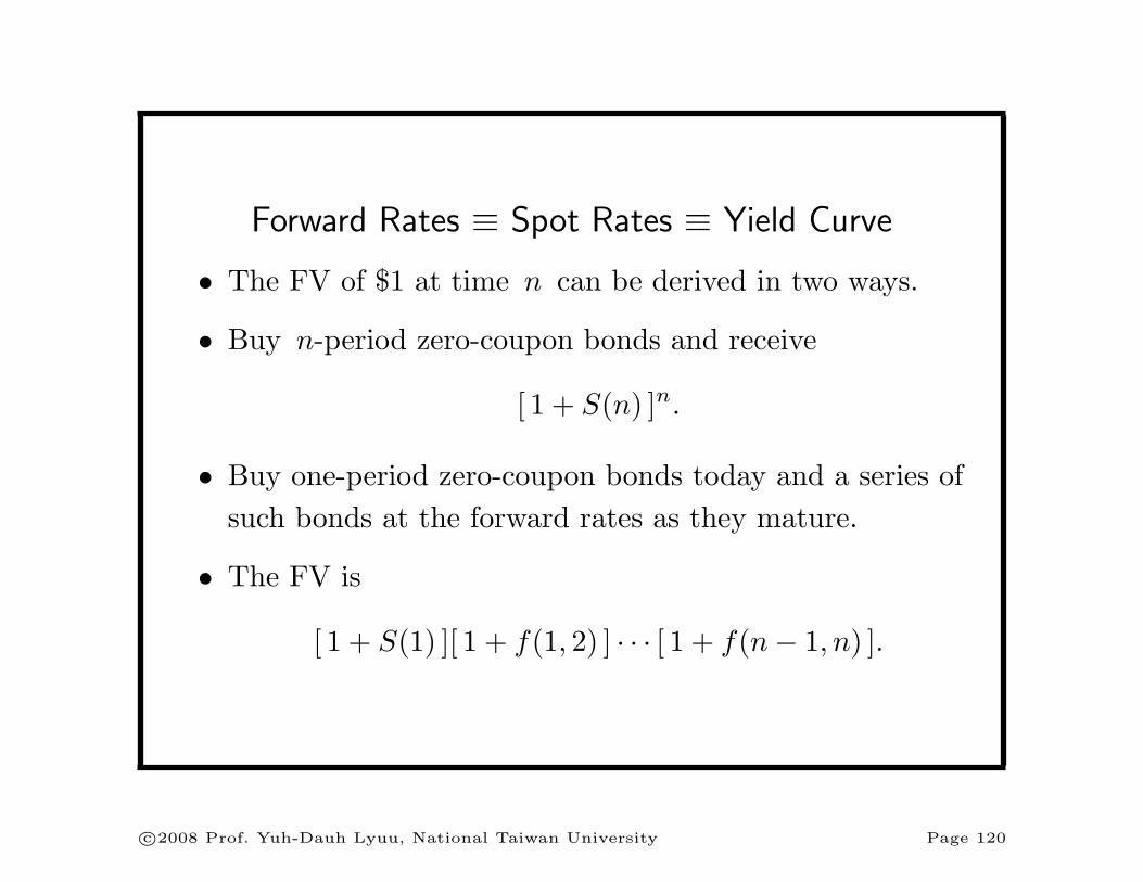
Forward Rates ≡ Spot Rates ≡ Yield Curve

• The FV of $1 at time n can be derived in two ways.

• Buy n-period zero-coupon bonds and receive

[ 1 + S(n) ]n.

• Buy one-period zero-coupon bonds today and a series ofsuch bonds at the forward rates as they mature.

• The FV is

[ 1 + S(1) ][ 1 + f(1, 2) ] · · · [ 1 + f(n− 1, n) ].


Forward Rates ≡ Spot Rates ≡ Yield Curves(concluded)

• Since they are identical,

S(n) = {[ 1 + S(1) ][ 1 + f(1, 2) ]

· · · [ 1 + f(n− 1, n) ]}1/n − 1. (12)

• Hence, the forward rates, specifically the one-periodforward rates, determine the spot rate curve.

• Other equivalencies can be derived similarly, such as

f(T, T + 1) =d(T )

d(T + 1)− 1.


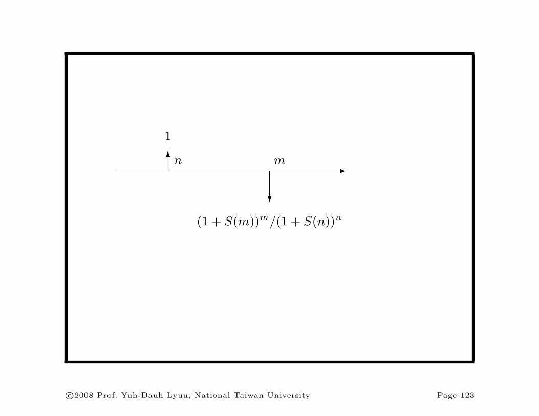
Locking in the Forward Rate f(n,m)

• Buy one n-period zero-coupon bond for 1/(1 + S(n))n.

• Sell (1 + S(m))m/(1 + S(n))n m-period zero-couponbonds.

• No net initial investment because the cash inflow equalsthe cash outflow 1/(1 + S(n))n.

• At time n there will be a cash inflow of $1.

• At time m there will be a cash outflow of(1 + S(m))m/(1 + S(n))n dollars.

• This implies the rate f(n,m) between times n and m.


-6

?

n m

1

(1 + S(m))m/(1 + S(n))n


Forward Contracts

• We generated the cash flow of a financial instrumentcalled forward contract.

• Agreed upon today, it enables one to borrow money attime n in the future and repay the loan at time m > n

with an interest rate equal to the forward rate

f(n,m).

• Can the spot rate curve be an arbitrary curve?a

aContributed by Mr. Dai, Tian-Shyr (R86526008, D8852600) in 1998.


Spot and Forward Rates under ContinuousCompounding

• The pricing formula:

P =n∑

i=1

Ce−iS(i) + Fe−nS(n).

• The market discount function:

d(n) = e−nS(n).

• The spot rate is an arithmetic average of forward rates,

S(n) =f(0, 1) + f(1, 2) + · · ·+ f(n− 1, n)

n.


Spot and Forward Rates under ContinuousCompounding (concluded)

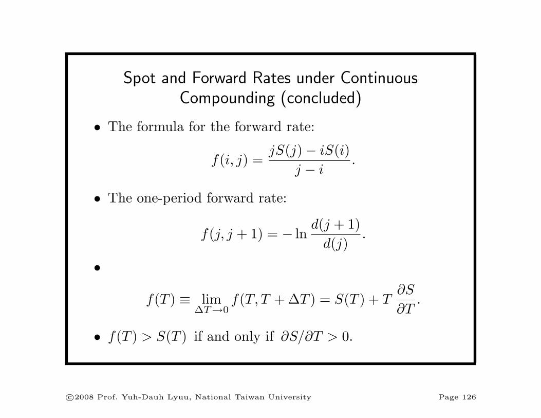
• The formula for the forward rate:

f(i, j) =jS(j)− iS(i)

j − i.

• The one-period forward rate:

f(j, j + 1) = − lnd(j + 1)

d(j).

•

f(T ) ≡ lim∆T→0

f(T, T + ∆T ) = S(T ) + T∂S

∂T.

• f(T ) > S(T ) if and only if ∂S/∂T > 0.


Unbiased Expectations Theory

• Forward rate equals the average future spot rate,

f(a, b) = E[ S(a, b) ]. (13)

• Does not imply that the forward rate is an accuratepredictor for the future spot rate.

• Implies the maturity strategy and the rollover strategyproduce the same result at the horizon on the average.


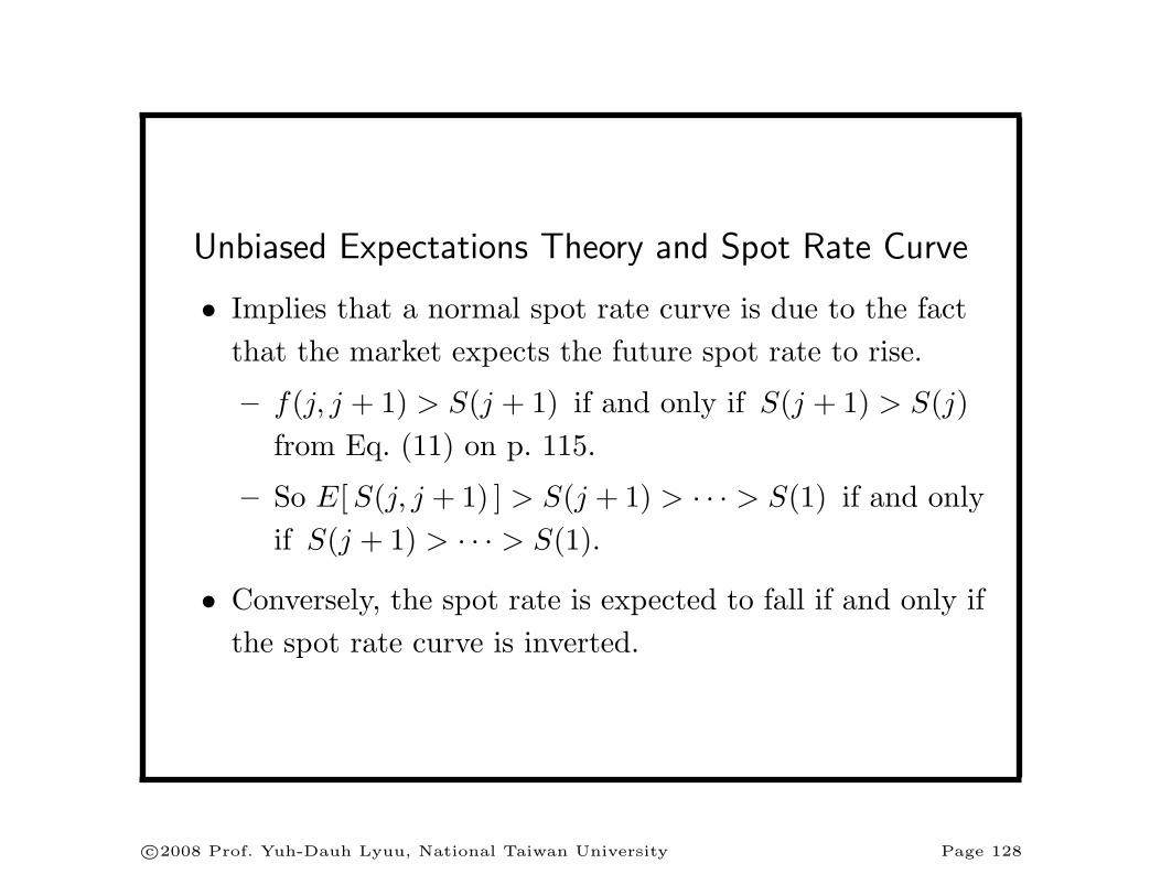
Unbiased Expectations Theory and Spot Rate Curve

• Implies that a normal spot rate curve is due to the factthat the market expects the future spot rate to rise.

– f(j, j + 1) > S(j + 1) if and only if S(j + 1) > S(j)from Eq. (11) on p. 115.

– So E[ S(j, j + 1) ] > S(j + 1) > · · · > S(1) if and onlyif S(j + 1) > · · · > S(1).

• Conversely, the spot rate is expected to fall if and only ifthe spot rate curve is inverted.


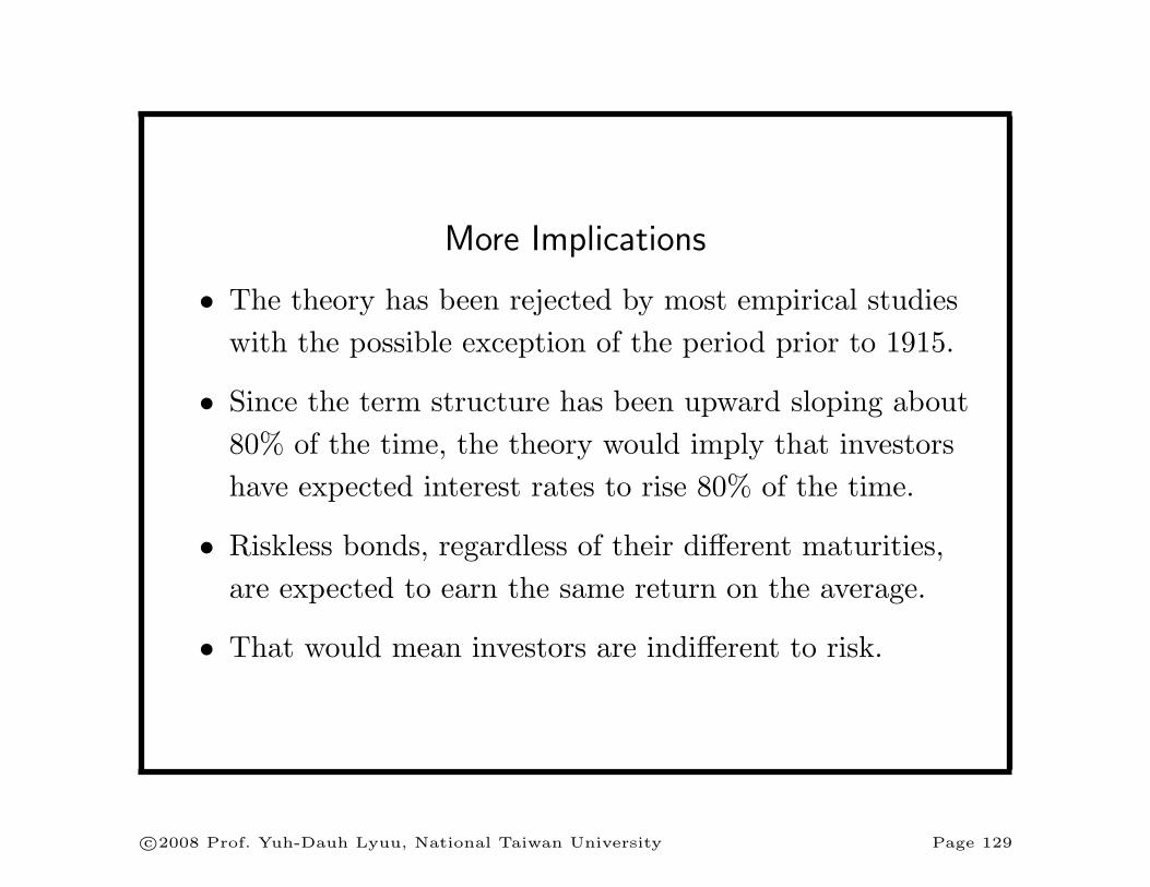
More Implications

• The theory has been rejected by most empirical studieswith the possible exception of the period prior to 1915.

• Since the term structure has been upward sloping about80% of the time, the theory would imply that investorshave expected interest rates to rise 80% of the time.

• Riskless bonds, regardless of their different maturities,are expected to earn the same return on the average.

• That would mean investors are indifferent to risk.


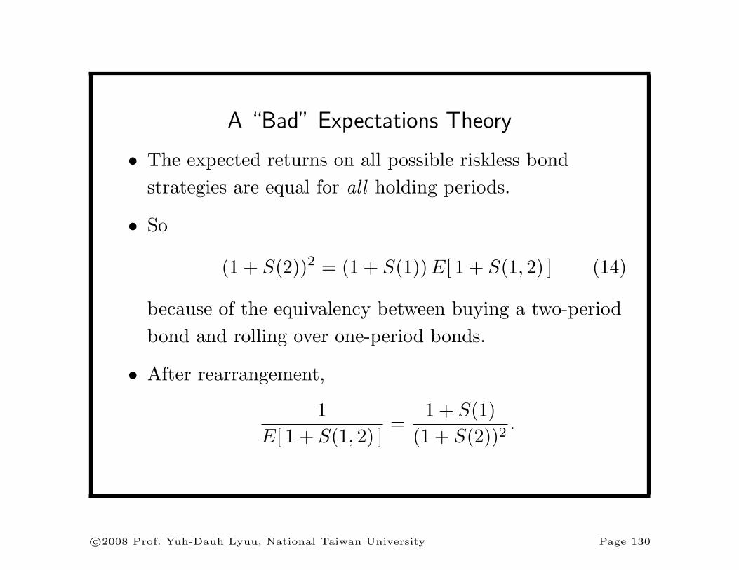
A “Bad” Expectations Theory

• The expected returns on all possible riskless bondstrategies are equal for all holding periods.

• So

(1 + S(2))2 = (1 + S(1)) E[ 1 + S(1, 2) ] (14)

because of the equivalency between buying a two-periodbond and rolling over one-period bonds.

• After rearrangement,

1E[ 1 + S(1, 2) ]

=1 + S(1)

(1 + S(2))2.


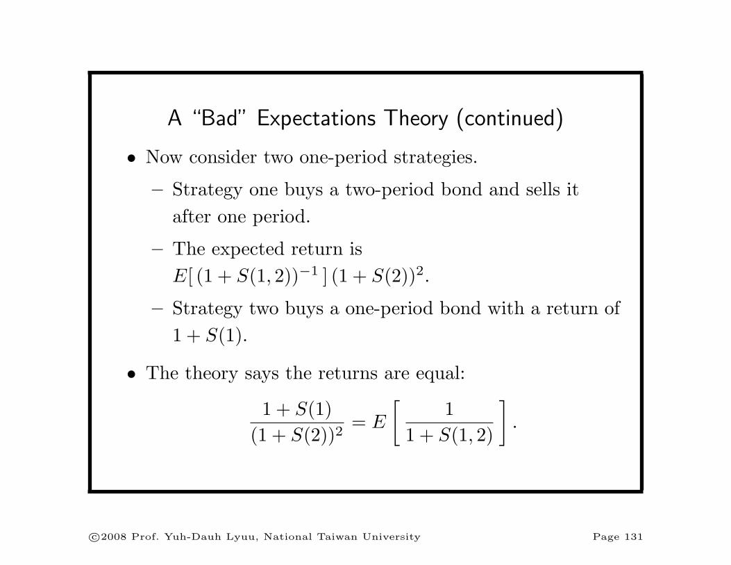
A “Bad” Expectations Theory (continued)

• Now consider two one-period strategies.

– Strategy one buys a two-period bond and sells itafter one period.

– The expected return isE[ (1 + S(1, 2))−1 ] (1 + S(2))2.

– Strategy two buys a one-period bond with a return of1 + S(1).

• The theory says the returns are equal:

1 + S(1)(1 + S(2))2

= E

[1

1 + S(1, 2)

].


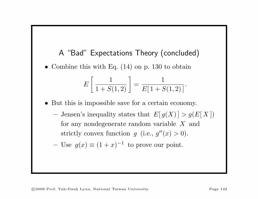
A “Bad” Expectations Theory (concluded)

• Combine this with Eq. (14) on p. 130 to obtain

E

[1

1 + S(1, 2)

]=

1E[ 1 + S(1, 2) ]

.

• But this is impossible save for a certain economy.

– Jensen’s inequality states that E[ g(X) ] > g(E[X ])for any nondegenerate random variable X andstrictly convex function g (i.e., g′′(x) > 0).

– Use g(x) ≡ (1 + x)−1 to prove our point.


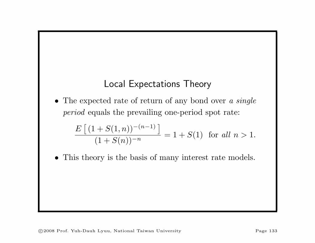
Local Expectations Theory

• The expected rate of return of any bond over a singleperiod equals the prevailing one-period spot rate:

E[(1 + S(1, n))−(n−1)

]

(1 + S(n))−n= 1 + S(1) for all n > 1.

• This theory is the basis of many interest rate models.


Duration Revisited

• To handle more general types of spot rate curve changes,define a vector [ c1, c2, . . . , cn ] that characterizes theperceived type of change.

– Parallel shift: [ 1, 1, . . . , 1 ].

– Twist: [ 1, 1, . . . , 1,−1, . . . ,−1 ].

– · · ·• Let P (y) ≡ ∑

i Ci/(1 + S(i) + yci)i be the priceassociated with the cash flow C1, C2, . . . .

• Define duration as

−∂P (y)/P (0)∂y

∣∣∣∣y=0

.


Documents

Bond Price Volatility - 國立臺灣大學lyuu/finance1/2008/20080227.pdf · † For a bond with positive convexity, the price rises more ... † In the bond price formula, Xn i=1