arX

iv:a

stro

-ph/

0105

148v

1 9

May

200

1

The Boomerang North America instrument: a balloon-borne

bolometric radiometer optimized for measurements of cosmic

background radiation anisotropies from 0.3 to 4.

F. Piacentini1, P.A.R. Ade2, R. Bathia3, J.J. Bock3,4, A. Boscaleri5, P. Cardoni6,

B.P. Crill3, P. de Bernardis1, H. Del Castillo4, G. De Troia1, P. Farese1, M. Giacometti1,

E.F. Hivon3, V.V. Hristov3, A. Iacoangeli1, A.E. Lange3, S. Masi1, P.D. Mauskopf3,7,

L. Miglio1,8, C.B. Netterfield3,8, P. Palangio9, E. Pascale3,5, A. Raccanelli1, S. Rao1,9,

G. Romeo9, J. Ruhl10, F. Scaramuzzi6

ABSTRACT

We describe the Boomerang North America (BNA) instrument, a balloon-

borne bolometric radiometer designed to map the Cosmic Microwave Background

(CMB) radiation with 0.3 resolution over a significant portion of the sky. This

receiver employs new technologies in bolometers, readout electronics, millimeter-

wave optics and filters, cryogenics, scan and attitude reconstruction. All these

subsystems are described in detail in this paper. The system has been fully

calibrated in flight using a variety of techniques which are described and com-

pared. Using this system, we have obtained a measurement of the first peak in

the CMB angular power spectrum in a single, few hour long balloon flight. The

instrument described here was a prototype of the Boomerang Long Duration

Balloon (BLDB) experiment.

1Dipartimento di Fisica, Universita’ La Sapienza, P.le A. Moro 2, 00185, Roma, Italy, e-mail:

francesco.piacentini@roma1.infn.it

2Department of Physics, Queen Mary and Westfield College, Mile End Road, London, E1 4NS, U.K.

3Department of Physics, Math, and Astronomy, California Institute of Technology, Pasadena, CA, USA

4Jet Propulsion Lab, Pasadena, CA, USA

5IROE-CNR, Via Panciatichi 54, 50127 Firenze, Italy

6Ente Nazionale Energie Alternative, Frascati, Italy

7Dept. of Physics and Astronomy, University of Massachusets, Amherst, MA, USA

8Department of Astronomy, University of Toronto, Canada

9Istituto Nazionale di Geofisica, Roma, Italy

10Dept. of Physics, Univ. of California, Santa Barbara, CA, USA

– 2 –

Subject headings: cosmology: observations — cosmic microwave background —

instrumentation: photometers

1. Introduction

The existence of the 2.7 K Cosmic Microwave Background (CMB) Radiation is evidence

that our universe originated from a hot, dense plasma (Hu et al. 1997). This radiation was

emitted in the early universe, when the plasma cooled enough for protons and electrons to

form hydrogen atoms. Before recombination, photons and baryons where tightly coupled by

Compton scattering. After recombination the photons and baryons are highly decoupled,

with a mean free path longer than the causal horizon. This event is dated ∼ 300000 years

after the Big Bang when the universe was ∼ 1000 times smaller and ∼ 50000 times younger

(red shift z=1000). The properties of the CMB reflect the conditions of the early universe

and are closely linked with global properties of the universe, such as the energy density

(Ωtot), composition (Ωb, ΩΛ, ΩDM), and expansion rate (H0).

In particular, variations in the brightness of the CMB, or anisotropies, reflect variations

in temperature, density, and velocity of the last scattering surface. These fluctuations, that

originated from random noise at an earlier phase of expansion, are the seeds for the formation

of structures such as galaxies and clusters of galaxies present in the universe today. Precise

measurements of the angular power spectrum of CMB anisotropies (White et al. 1994) will

discriminate between competing cosmological models and, if the inflationary scenario is

correct, will accurately determine many of the physical parameters of the universe.

The COBE-DMR detection (Smoot et al. 1991; Smoot et al. 1992) of anisotropies in

the CMB at large angular scales provides a point of reference for theoretical models of the

origin of fluctuations in the CMB (Bond et al. 1994). Measurements at smaller angular

scales are needed to fully understand the nature of these fluctuations. Since the launching

of COBE, many other experiments have made significant detections of CMB anisotropy at

a wide variety of angular scales, from 0.3 to 10, but until 1998, none of the measurements

provided enough information for serious cosmological parameter determination.

The new generation of CMB experiments is designed to probe models of structure for-

mation with a combination of higher sensitivity, sky coverage and resolving power. Advances

in detector technology have resulted in radiometers that are over 100 times more sensitive

than the COBE-DMR per unit time. In addition, improved techniques for removing noise

from atmospheric fluctuations with both single dish instruments and interferometers allow

increased sensitivity with ground-based telescopes. Long Duration Balloon (LDB) platforms

– 3 –

provide the opportunity to obtain the long integration times needed for large sky coverage

with balloon-borne telescopes.

Boomerang is an experiment designed to measure the detailed structure of the CMB

at angular scales from 0.2 to 4 with high sensitivity. The Boomerang instrument consists

of a 1.3 m balloon-borne telescope and pointing platform with a 300 mK bolometric array

receiver. The receiver is contained inside a liquid Nitrogen (LN2) and liquid Helium (LHe)

cryostat with a hold-time of two weeks.

The measurement technique consists of measuring a sky brightness map by slowly scan-

ning the telescope (and the full payload) in azimuth, using the earth rotation to cover a wide

sky region. There is no mechanical chopper. The scan converts CMB anisotropies at differ-

ent angular scales into detector signals at different sub-audio frequencies. The instrument

features a new total power readout of the detectors, optimized to preserve the information

content of the signal while rejecting very low and very high frequency noise. This approach

pioneers in several aspects the HFI instrument on the Planck satellite.

In this paper we describe the instrument prototype as it was used for the test flight,

on Aug.30, 1997, to qualify all the flight subsystems for later use in the Antarctic LDB

flight. During the 1997 test flight we observed about 200 square degrees of sky at high

Galactic latitudes. Science results from that flight are reported in (Mauskopf et al. 2000)

and (Melchiorri A. et al. 2000). Here we give all the technical details of the instrument as

well as its performance during the test flight: thermal performance, bolometer loading and

noise, scan performance, attitude reconstruction, calibration on Jupiter and on the CMB

Dipole. The LDB instrument is described in (Crill et al. 2001).

2. Instrument

Boomerang is designed to take advantage of the long integration time possible from

a balloon borne platform flown over the Antarctic. Antarctic summer ballooning is very at-

tractive for CMB anisotropy experiments for two reasons. The first is that the flight duration

(up to ∼ 20 days) allows for substantial sky coverage and deep checks for systematics; the

second is that very low foreground regions are observable in the direction generally opposite

the sun during the Antarctic summer.

There are, however, a number of challenges peculiar to Antarctic ballooning. The long

flight duration requires special cryogenic systems. The cosmic ray flux in polar regions is

enhanced by a factor of about ten with respect to North American latitudes, thus resulting

in a high noise in standard bolometric detectors. The continual presence of the sun during

– 4 –

an Antarctic LDB flight is a general concern for the thermal performance of the payload and

for pickup in the sidelobes of the telescope. The balloon is far from the ground equipment,

so special data collection and telemetry systems have to be used, and interactivity with the

system is reduced.

We describe in the following the solutions we have adopted to overcome these prob-

lems, developing custom subsystems: a long duration cryostat, spider-web bolometers, low

sidelobes off-axis optics, special sun shields and telescope baffling, total power readout.

A general view of the experiment with its main subsystems is shown in Figure 1.

Fig. 1.— Boomerang payload. Special shields in aluminized mylar protect from sun and

earth radiation reducing sidelobes. Radiation coming from the sky is reflected into the

cryostat by means of the 1.3 m primary mirror. Solar panel are used for power supply in

the LDB flight while Lithium batteries ware used in the BNA flight. The Attitude Contol

System (ACS) provides pointing and scanning of the telescope.

– 5 –

2.1. Optics

The Boomerang telescope consists of an ambient temperature 1.3 m diameter off-axis

parabolic primary mirror (f=1280 mm, 45 off-axis) which feeds cold reimaging secondary

and tertiary mirrors inside a large liquid helium cryostat. The telescope and the cryostat are

both mounted on an aluminum frame (the inner frame of the payload) which can be tipped in

elevation by −12 to +20 to cover elevation angles from 33 to 65. The primary mirror has

a 45 off-axis angle. Radiation from the sky is reflected by the primary mirror and enters the

cryostat through a thin (50 µm) polypropylene window near the prime focus. Two circular

windows side by side, each 66 mm in diameter, are used. This geometry provides a wide field

of view while allowing the use of thin window material which minimizes the emission from

this ambient temperature surface. Filters rejecting high frequency radiation are mounted on

the 77 K and 2 K shields in front of the cold reimaging optics. Fast off-axis secondary and

tertiary mirrors surrounded by absorbing baffles reimage the prime focus onto the detector

focal plane.

The Boomerang optics (Figure 2) is optimized for an array with widely separated

pixels. The advantage of having large spacing between pixels in the focal plane is the ability

to difference (or compare) the signals from two such pixels and remove correlated optical

fluctuations such as temperature drift of the telescope, while retaining high sensitivity to

structure on the sky at angles up to the pixel separation. This scheme eliminates the need

for moving optical components and simplifies the design and operation of the experiment.

We optimized the optics for diffraction limited performance at 1 mm over a 2 × 5

field of view. The reimaging optics are configured to form an image of the primary mirror

at the 10 cm diameter tertiary mirror. The size of the tertiary mirror therefore limits the

illumination pattern on the primary mirror, which is underfilled by 50% in area (85 cm in

diameter) to improve sidelobe rejection.

The secondary mirror is an ellipsoid and the tertiary is a paraboloid, 10 cm in diameter,

corresponding to an 85 cm diameter aperture on the 1.3 m primary mirror. The equation

describing the three mirrors is

z(r) =r2

R

[

1 +√

1− (1 + k) r2

R2

] + Ar4 +Br6 (1)

with parameters R, k, A, B as in Table 1.

The BNA focal plane contains single frequency channels fed by conical or Winston

horns. Although the image quality from the optics is diffraction limited over a 2 × 5 field,

all of the feed optics are placed inside two circles 2 in diameter, separated by 3.5 center

– 6 –

Fig. 2.— Boomerang optics. Secondary and tertiary mirrors project the image on the

focal plane. They are cooled to 2 K inside the main cryostat. An image of the 1.3 m primary

mirror is formed on the tertiary mirror which works as a cold Lyot stop, improving the

off-axis rejection of the photometer.

to center. The focal plane area outside these circles is vignetted by blocking filters at the

entrance to the optics box and on the 77 K shield and is unusable. Due to the curvature of

the focal plane, the horns are placed at the positions of the beam centroids determined by

geometric ray tracing. All of the feeds are oriented towards the center of the tertiary mirror.

The configuration of the focal plane for the North American Flight is in Figure 3.

The BNA frequency bands are centered at 90 and 150 GHz and are optimized to max-

imize sensitivity to CMB fluctuations, identify dust emission and reject radiation from at-

mospheric line emission. The low pass filters mounted on the 77 K and 2 K optical entrance

windows provide good transmission across these bands while effectively blocking higher fre-

quency radiation. Two metal mesh low pass filters with cutoff frequencies of 480 GHz are

mounted on the 77 K stage. The filters are 65 mm in diameter and each one is directly

– 7 –

Mirror R (mm) k A (mm−3) B (mm−5)

Primary 2560 -1.0 0.0 0.0

Secondary 363.83041 -0.882787413818 1.3641139×10−9 1.8691461×10−15

Tertiary 545.745477407 -1.0 4.3908607×10−10 -3.2605391×10−15

Table 1: Ideal parameters for the equation of the three Boomerang mirrors (see eqn.1)

behind one of the 50 µm polypropylene vacuum windows. Two more low pass filters with a

cutoff frequency of 300 GHz are mounted on the 2 K stage at the entrance to the cold optics

box. Although each filter has a leak at twice the cutoff frequency, the combination eliminates

these leaks. Because these filters are reflective at frequencies above the cutoff, they minimize

the radiation heat load on the cryogens. While the metal mesh filters have high reflectivity

at high frequencies, they are not impenetrable, and above a few THz any transmission at

the level of less than 10−3 is significant. Therefore, we place a dielectric absorber behind

the 300 GHz filter on the 2 K stage that has a cutoff frequency of 1650 GHz. The absorber

is 0.5 mm thick alkali-halide filter coated with a 130 µm thick layer of black polyethylene.

This low pass filter stack has a transmission of > 80% at all frequencies from 90 to 410 GHz,

while attenuates by a factor 5 · 10−4 between 1650 GHz and 100 THz and by a factor 10−3

over 100 THz. All of the other filtering is done in the focal plane elements.

We have produced two different feeds designed to efficiently couple to the telescope and

produce beam sizes on the sky of 20′ and 40′. These sizes are larger than the diffraction

limit: we traded resolution for throughput to obtain good sensitivity to diffuse radiation

even in a short test flight. The design of the single frequency feed structure is shown in

Figure 4 and is similar to the feed design described in (Church et al. 1996). This design

allows us to illuminate correctly the band defining filters and create an effective Faraday

cage surrounding the bolometric detectors.

Each feed consists of a band defining filter stack mounted inside waveguide optics that

couple the radiation from the tertiary mirror into an integrating bolometer cavity. The feed

is divided in two parts separated by a 0.5 mm gap, one held at 2 K and the other at 300 mK.

The entrance horns are mounted in a horn positioning flange held at 2 K. Each horn

couples to a section of waveguide with length 2λ that acts as a high pass filter and rejects

radiation with wavelength λ > 3.41a, where a is the radius of the waveguide. The 20′ horns

have an entrance aperture of 19.7 mm at f = 3.3 and a waveguide diameter of 2.54 mm. The

throughput is limited by a combination of the entrance aperture of the horns and the size of

the Lyot stop to be AΩtotal = 0.1 cm2sr for the 20′ horns. This value is over the diffraction

limit throughput AΩhorn ≃ λ2 = 0.04 cm2sr at λ ≃ 2 mm (150 GHz). The 40′ horns have

– 8 –

Fig. 3.— Location of the beams in the focal plane of the BNA photometer.

an entrance aperture of 33 mm and a waveguide diameter of 5.1 mm. These channels have

approximately three times the throughput of the 20′ channels with AΩ ≃ 0.3 cm2sr, while

the diffraction limit is 0.1 cm2sr.

On the other side of the waveguide is an f/4 conical horn that expands the waveguide to

a diameter of 17.8 mm in the 20′ channel and 27.9 mm in the 40′ channel. At the end of this

cone, the feed opens up to allow the mounting of a converging lens and an oversized metal

mesh dichroic filter. A band pass filter followed by another identical converging lens and

conical horn are held at 300 mK across the small gap of < 1 mm. This final horn feeds a small

cavity containing a micromesh bolometer which absorbs > 90% of the radiation entering the

cavity. In the geometrical limit, the lenses reimage to infinity a point at the vertex of the

horns on which they are mounted. In the diffraction limit, they each produce a beam waist

at the center of the length of waveguide that contains the filters, thereby improving the

coupling between the expanding horn at 2 K and the concentrating horn at 300 mK.

The spectral bands are defined by the 300 mK band pass filters, metal-mesh resonant

grid filters with nominal central frequencies of 90 GHz and 150 GHz and 30% bandwidth.

– 9 –

Fig. 4.— 150 GHz feed horn. The upper part is cooled at less than 2 K and the lower part

to 0.280 K. See text for description.

These filters have high transmission in band with sharp band edges, but their performance

degrades quickly as a function of off-axis angle. The f/4 horns in the intermediate section of

the feed structure insure that the filters are illuminated with small off-axis angles. The band

pass filters also have a leak at approximately twice the central frequency. The 2 K dichroic

filters in the feed structure eliminate these leaks and provide additional high frequency

blocking with cutoff frequencies of 172 GHz for the 90 GHz channel and 217 GHz for the

150 GHz channel. The frequency response of a 90 GHz and a 150 GHz channel, measured

with a Fourier Transform Spectrometer, are shown in Figure 5. The out-of-band transmission

is < −25 dB for ν < 900 GHz.

We have measured the optical efficiency of this structure equipped with filters for both

90 GHz and 150 GHz operation. The optical efficiency measurements were made using black

– 10 –

100 150 2001E-3

0.01

0.1

1

90 GHz 150 GHz

spec

tral

eff

icie

ncy

frequency (GHz)

Fig. 5.— Frequency response of a 90 and a 150 GHz channel as measured with a Fourier

Transform Spectrometer.

loads of eccosorb foam at 77 K and 300 K. We measure the difference in optical power on

a bolometer by comparing the DC-coupled I-V curves of the detector under the different

loading conditions. Pre-flight results are in Section 5.

Tables 2 and 3 give the band centroids and widths for the Boomerang photometers,

along with the estimated loadings from the CMB, the telescope, and the atmosphere.

2.2. Detectors

Boomerang uses bolometers to detect the fluctuations in incoming radiation. A

bolometer consists of a broadband absorber with heat capacity C, that has a weak thermal

link G, to a thermal bath at a temperature Tb. Incident radiation produces a temperature

rise in the absorber that is read out with a current biased thermistor. The sensitivity of a

bolometer expressed in Noise Equivalent Power (NEP) is given by:

NEPbolo = γ√

4kTb2G (2)

– 11 –

νnominal νpeak νCMB0 νR−J

0 ∆νFWHM

(GHz) (GHz) (GHz) (GHz) (GHz)

90 88.5 93.6 94.1 33

150 136.5 155.7 157.9 54

Table 2: Boomerang North America Filter Bands. νpeak is the peak for a flat spectrum,

νCMB0 and νR−J

0 are respectively the peaks for a CMB and a Rayleigh-Jeans spectra.

νpeak AΩ Patm PCMB Ptel

(GHz) cm2sr (pW) (pW) (pW)

BOOM/NA 88.5 0.3 0.004 0.10 0.42

136.5 0.1 0.28 0.17 1.6

Table 3: Boomerang/NA in flight expected loadings

where γ is a constant of order unity that depends weakly on the sensitivity of the thermistor

and k is Boltzmann’s constant. The dynamical equation for the temperature of the thermistor

can be expressed as:dTbolo

dt=

Pin −G(Tbolo − Tb)

C(3)

where Pin is the incident power. From this equation, we can see that bolometers have a

finite bandwidth limited by the time for the absorber to come to equilibrium after a change

in incident power, τ = C/G. Previous balloon-borne bolometric receivers have been limited

in sensitivity or bandwidth by the properties of the materials used for fabrication of the

detectors.

Bolometers are also limited in sensitivity by external sources of noise such as cosmic

rays, microphonic disturbances, and Radio Frequencies Interference (RFI). Of particular

importance for Boomerang is the cosmic ray rate on the Antarctic stratosphere, which is

about an order of magnitude higher than at North American latitudes because the magnetic

field of the earth funnels charged particles to the poles. We have experience of cosmic ray hits

from many bolometric receivers flown at balloon altitude at temperate latitudes. The cosmic

ray hit rate for the MAX experiment (Alsop et al. 1992) during a North American balloon

flight was 0.14 Hz. In order to remove spurious signals from these cosmic ray interactions,

cosmic rays were identified and a length of data corresponding to 10 detector time constants

was removed. Because the MAX detector time constants were all less than 30 ms, this

resulted in a loss of 5% of the data which did not severely affect the sensitivity. Almost half

of the data would be contaminated by cosmic rays with the same detectors operated from a

– 12 –

Long Duration Balloon over the Antarctic.

In the North American flight of Boomerang we tested for the first time bolometers

with a new architecture, consisting of a micromesh absorber with an indium bump-bonded

NTD germanium thermistor. These bolometers can have lower heat capacity, lower thermal

conductivities, lower cosmic ray cross section, and less sensitivity to microphonic heating

than previous 300 mK bolometers. The micromesh absorbers and support structures are

fabricated from a thin film of silicon nitride using microlithography. The absorber is a

circular grid with 60-400 µm grid spacing and 2-10% filling factor, metallized with 50 A

of chromium and 200 A of gold. It is designed to efficiently couple to millimeter wave

radiation and have low heat capacity and low cosmic ray cross section. Stiff mechanical

support consists in strands of silicon nitride 1000 µm long with 3-5 µm2 cross sectional

area connecting the absorber to a silicon frame, with a thermal conductivity of less than

2× 10−11 W K−1. The design and construction of the micromesh absorbers as well as their

optical and mechanical properties are described in (Mauskopf et al. 1997).

The thermistor is a rectangular prism of Neutron Transmutation Doped germanium

50 µm × 100 µm × 300 µm, a factor of 10 times smaller volume than NTD themistors

typically used in composite bolometers. Using these small thermistors decreases the heat ca-

pacity of the bolometer by a factor of 5 and increases the fundamental microphonic frequency

by a factor of 10. To allow the thermistor to be indium bump-bonded to the micromesh,

one of the long faces of the NTD material is metallized with two pads 50 µm wide at either

end. Each pad is first implanted with boron and then sputtered with 200 A of palladium

and 4000 A of gold. Electrical leads, gold pads, and indium bumps are patterned on the

micromesh while the silicon nitride still has a solid backing of silicon. Gold pads and indium

bumps are deposited at the center of the micromesh on a 300 µm × 300 µm solid square

of silicon nitride. For electrical leads, 200 A of gold is deposited on some of the support

legs of the silicon nitride connecting the pads for the thermistor with large gold pads on the

silicon frame. The thermistor is pressed onto the indium bumps and finally the silicon is

etched from the back of the micromesh. The front of the silicon nitride is coated in wax to

protect the chip and the metallization during etching. This technique minimizes the amount

of material used for reading out the thermistors and therefore minimizes the heat capacity

of the device. The indium bump-bonds have survived repeated thermal cycling. A draw of

a micromesh bolometer is shown in Figure 6. The performance of bolometers with indium

bump-bonded thermistors is described in (Bock et al. 1996).

– 13 –

Fig. 6.— Schematic draw of a micromesh spider web bolometer absorber.

2.3. Readout Electronics

Most bolometric detectors in use today employ a high-impedence semiconductor ther-

mistor biased with a constant current. JFET preamplifiers have been used to provide a

combination of low voltage and current noise well matched to typical bolometer impedences

(Halpern 1986), but exhibit excess voltage noise at frequencies typically below a few Hz and

have limited the achievable bandwidth of these DC biased bolometers. At lower frequen-

cies, drifts in the bias current, drifts in the temperature of the heat sink, and amplifier gain

fluctuations have been expected to limit the ultimate stability of single bolometer systems.

AC bridge circuits have been successfully used in many experiments to read out pairs

of bolometers with stability to 30 mHz (Wilbanks et al. 1990; Devlin et al. 1994). In this

scheme a pair of detectors is biased with an alternating current so that resistance fluctuations

are transfomed into changes in the AC bias amplitude across each detector. These signals are

differenced in a bridge, amplified and demodulated. The AC signal modulation eliminates

the effects of 1/f noise in the preamplifiers since the resulting signal spectrum is centered

about the carrier frequency. The effects of drifts in the bias amplitude, amplifier gain,

and heat sink temperature are greatly reduced if the two detectors in the bridge are well

matched. The optical responsivity of each of the detectors in the bridge is equivalent to

that of a detector biased with the same rms DC power and is constant in time as long as

– 14 –

the average power on the detector is constant over the course of one detector thermal time

constant.

Boomerang employs an AC stabilized total power readout system for individual bolome-

ters, mounted on a temperature regulated stage (Hristov et al. 2001a). The circuit is sum-

marized in Figure 7.

Fig. 7.— Block diagram of the bolometers readout electronics (one channel shown). The

bolometer is AC biased with a differential, low-pass filtered square wave at ∼500 Hz. The AC

voltage across the bolometer is modulated by the resistance variations induced by changes

in the microwave power absorbed. A matched pair of low noise J-FETs inside the cryostat

reduce the signal impedance from ∼ 10MΩ down to ∼ 1kΩ; the signal is then amplified

by a differential preamp (AD624), band-pass filtered to remove noise outside the signal

bandwidth, and synchronously demodulated by a phase sensitive detector (AD630). The

output of the AD630 is proportional to the instantaneous resistance of the bolometer. Signal

components below 10 mHz are attenuated to get rid of 1/f noise and drifts using a single

pole high pass filter. High frequencies (above 10 Hz, i.e. above the cutoff frequency of the

bolometer) are also removed by means of a 4-th order low-pass filter. The resulting signal is

analog to digital converted with 16 bits resolution, at a sampling frequency of 62.5 Hz.

This system contains a cold J-FETs input stage (based on Infrared Laboratries TIA)

and contributes less than 10 nVrms/√Hz noise at all frequencies within the bolometer signal

bandwidth down to 20 mHz. The warm readout circuit has a gain stability of < 10 ppm/C.

We remove the large offset due to the background power on the detector with a final stage

high pass filter with a cutoff frequency of 16 mHz. With this circuit, we have measured the

noise spectrum of a low background micromesh bolometer with NEP = 1.2×10−17 W/√Hz,

biased for maximum responsivity to be flat down to a frequency of 20 mHz.

– 15 –

2.4. RF Filtering

There are many sources of Radio Frequency Interference (RFI) on the balloon that

could couple to bolometers. Microwave transmitters (400 MHz to 1.5 GHz, few W) that

send the data stream to the ground and high current wires that drive the motors of the

Attitude Control System (20 kHz PWM, several Amps) are situated within a few meters of

the cryostat. The Boomerang wiring and focal plane are designed to prevent RFI from

contributing to the noise of the bolometers.

The bolometers are contained inside a 2 K Faraday cage inside the cryostat. RFI can

enter the cryostat through the optical entrance window and propagate into the 2 K optics

box. However, the exit aperture of the optics box is RF sealed by the horn positioning plate.

This plate contains feed horns with small waveguide apertures for radiation from the sky

to pass through to the detectors. The largest waveguide feedthrough in this plate is 5.1

mm in diameter which corresponds to a waveguide cutoff of ∼ 35 GHz. Lower frequency

RFI is reflected by this surface. Readout wires entering the bolometer Faraday cage can

also propagate RF signals as coaxial cables. We run all of the bolometer wires through cast

eccosorb filters mounted to the wall of the Faraday cage to attenuate these signals. The

filters are 30 cm long and have a measured attenuation of < −20 dB at frequencies from

20 MHz to a few GHz.

The readout electronics are also sensitive to RFI. We enclose all of the cryostat elec-

tronics in an RF tight box that forms an extension of the outer shell of the cryostat. The

signals from the detectors pass through flexible KF-40 hose that is RF sealed to the hermetic

connector flange on the cryostat and to the wall of the electronics box. The amplified signals

exit the electronics box through Spectrum RF filters mounted on the wall of the box.

2.5. Cryogenics

A “heavy duty” 3He fridge and a large 4He cryostat have been developed specifically for

the Boomerang experiment. A cutaway view of the cryostat is shown in Figure 8.

The main 4He cryostat has to be large enough to contain refocusing optics and a wide

focal plane with several multiband photometers. The design and performance of the cryostat

and refrigerator are described in detail elsewhere (Masi et al. 1998; Masi et al. 1999). The

total volume occupied by the cryogenic section of the receiver is 69 liters. The design hold

time is about 20 days; the helium tank volume is 60 liters, the nitrogen tank volume is

65 liters. Conduction thermal input is reduced by suspending both the tanks with Kevlar

ropes (1.6 mm diameter). The vibration frequencies of these structures are all above 20 Hz,

– 16 –

Fig. 8.— Main cryostat. The evaporating 4He gas flow through the serpentine and the heat

exchanger to cool a copper shield that minimize the heat input on the main Helium bath.

The tanks are supported by kevlar cord. Nitrogen lines are not shown.

and the amplitude of the vibrations excited during the flight is expected to be very small.

Radiation thermal input on the nitrogen tank is reduced by means of 30 layers of aluminized

mylar for superinsulation. The total thermal input on the nitrogen bath is 6.6± 0.4 W.

The radiative thermal load on the L4He is minimized by the use of a vapor cooled shield.

As the liquid helium evaporates, the cold gas flows through a spiral tube that is soldered to

the outside of a copper shield which surrounds the Helium tank and through a copper heat

exchanger that is attached to the top of the vapor cooled shield before emerging from the

cryostat. The temperature of the vapor cooled shield depends on the gas flow rate from the

Helium tank. During normal operation, the shield remains at a temperature of 15-17 K. The

total thermal input on the helium bath is linked to the radiative input through the cryostat

window and in flight conditions is about 75 mW.

The cryostat has two circular windows 66 mm in diameter, made with 50 µm polypropy-

lene supported by an aluminum frame.

– 17 –

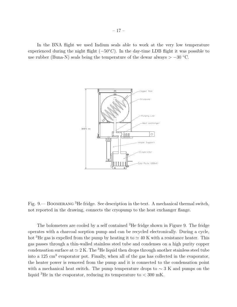
In the BNA flight we used Indium seals able to work at the very low temperature

experienced during the night flight (−50C). In the day-time LDB flight it was possible to

use rubber (Buna-N) seals being the temperature of the dewar always > −30 C.

Fig. 9.— Boomerang3He fridge. See description in the text. A mechanical thermal switch,

not reported in the drawing, connects the cryopump to the heat exchanger flange.

The bolometers are cooled by a self contained 3He fridge shown in Figure 9. The fridge

operates with a charcoal sorption pump and can be recycled electronically. During a cycle,

hot 3He gas is expelled from the pump by heating it to ≃ 40 K with a resistance heater. This

gas passes through a thin-walled stainless steel tube and condenses on a high purity copper

condensation surface at≃ 2 K. The 3He liquid then drops through another stainless steel tube

into a 125 cm3 evaporator pot. Finally, when all of the gas has collected in the evaporator,

the heater power is removed from the pump and it is connected to the condensation point

with a mechanical heat switch. The pump temperature drops to ∼ 3 K and pumps on the

liquid 3He in the evaporator, reducing its temperature to < 300 mK.

– 18 –

The pump is made of two stainless steel hemispheres crossed by a copper rod that

extends outside, to provide thermal attachment points to both the heater and the thermal

switch. The pump is connected to the copper condensation plate (∼ 2 K) through a 1 cm

diameter stainless steel tube. There is a 1 cm diameter hole that horizontally passes through

the condensation plate, with a 1 cm path to provide more surface area to transfer heat from

the 3He gas to the copper. The evaporator consists of a stainless steel cylinder with a 6 cm

diameter copper endcap with a ring of 6 mm diameter bolt holes for thermal attachment.

The charge is 34 liters STP at 40 bars. The heat load on the 3He stage is about 20 µW.

About half of this is due to thermal conduction from the condensation point to the evaporator

through the 0.010” diameter stainless steel pump tube. The remaining 10 µW is from the

mechanical supports for the focal plane. The focal plane weighs 2.5 Kg and must be rigidly

held with a mounting structure strong enough to withstand 10 G acceleration in any direction

while providing minimal additional thermal input to the 3He fridge. We use four thin-walled

vespel tubes to satisfy these requirements. Vespel has an extremely high strength to thermal

conductivity ratio at temperatures from 0.3 to 2 K. The tubes are 1” in diameter, 0.030”

thick and 3” long. The yield strength of a tube can be calculated from standard formulae.

The criterion we use for strength is that the maximum deflection be less than 1% of the

elastic limit of the material. Additional heat load from electrical leads is minimized by the

use of 0.005” diameter manganin wires that run up the length of the vespel tubes between

the cold JFET amplifier box and the detectors. The wires are firmly attached to fixed

surfaces along their entire length with teflon tape to eliminate vibrations which can make

the detectors microphonically sensitive. The length of the wires is minimized to reduce their

contribution to the input capacitance at the JFETs. The RC cutoff frequency for a 5 MΩ

detector impedence is measured to be > 2 kHz, for an input capacitance of < 40 pF.

During observations, the temperature of the focal plane can be maintained constant with

a high precision temperature regulation circuit (Hristov et al. 2001b). In fact, temperature

fluctuations of the 300 mK stage can contribute to excess bolometer noise. The temperature

of the bolometer is determined by:

Tbolo = T0 +Popt

∫ Tbolo

T0κ0TαdT

(4)

where Popt is the optical power on the detector and∫ Tbolo

T0κ0T

αdT, indicated as Geff (W K−1)

hereafter, is the effective thermal conductivity per unit of temperature between the thermis-

tor and the bath at T0. Therefore the change in bolometer temperature for a change in base

plate temperature is given by:

∆Tbolo = β∆T0 (5)

where β is a constant of order unity. The bolometer NEP is related to these temperature

– 19 –

fluctuations by:

NEPT = Geff∆Tbolo (6)

where NEPT is in W/√Hz and ∆Tbolo (K/

√Hz) is the spectrum of temperature fluctuations.

Therefore, the condition for temperature stability of the cold stage is NEPT < NEPbolo. For

the Boomerang bolometers with Geff = 8×10−11 W K−1 and NEPbolo ≃ 2×10−17 W/√Hz

the requirement for the stability of the cold stage is:

∆Tbolo < 250nK/√Hz (7)

Two NTD thermistors are mounted on the 300 mK stage and read out with DC cou-

pled bridge circuits. One channel is used as the control sensor and the other is a monitor

sensor. We measure the spectrum of fluctuations from the monitor channel while the tem-

perature regulation circuit is running to be flat down to < 30 mHz with an amplitude of

40 µVrms/√Hz corresponding to a temperature stability of 120 nK/

√Hz. This is better

than is needed to insure that the Boomerang bolometers do not have a significant noise

contribution from temperature fluctuations.

2.6. Pressure control systems

The pressure on the main helium bath is maintained around 10 mbar in lab and in flight

to keep the bath temperature below 2 K, while the pressure on the nitrogen bath is kept

around 1 atm to prevent the formation of fluffy solid. We used two pressurization systems.

The helium pressurization system allows us to pump on the bath at ground and to open to

atmosphere pressure at float by means of a motorized high vacuum seal valve. The nitrogen

system controls the pressure using an absolute sensor and three electrovalves. Both systems

have relief valves to allow safety and functionality even in the case of electronic failures.

2.7. Internal calibrator

An internal calibrator in the reimaging optics box allows us to monitor the detector

sensitivity during flight. The calibrator consists of a high background bolometer with an

NTD 4 Ge thermistor attached to the center of a 5.6 mm diameter Silicon Nitride absorber,

electrically connected with 0.001” diameter copper leads. The calibrator is mounted on the

2 K stage directly behind a 1 cm hole in the center of the tertiary mirror, where all of the

beams from the concentrating horns are coincident. The calibrator can be heated with a

current pulse to give a temperature rise of several Kelvin with a recovery time of a few

– 20 –

milliseconds. The corresponding power on the detectors is:

Pcal ≃ 2k∆Tcal

ν2

c2∆ν · Ωǫf (8)

where ǫ is the calibrator efficiency and f is the effective Lyot stop fraction area filled by the

calibrator. This corresponds to an equivalent signal on the sky of

∆TCMB = ǫ∆Tcalf (9)

Response to the internal calibrator during flight for one of the detectors is shown in Figure 10.

The equivalent signal on the sky is ∼ 175 mK.

0 2 4 6 8Time (sec)

-2.0•103

0

2.0•103

4.0•103

6.0•103

8.0•103

1.0•104

1.2•104

Sig

nal (

A2D

uni

ts)

B15

0B2

Fig. 10.— Bolometer signal during a pulse from the internal calibrator. A/D units are used,

corresponding to a full scale of ±10 Volts in 16 bits.

3. Attitude Control System

The Attitude Control System (ACS) must be able to point in a selected sky direction,

and track it or scan over it with a reasonable speed. The specifications are 1 arcmin rms

for pointing stability, with a reconstruction capability better than ∼ 0.5 arcmin maximum.

Our main modulation is obtained scanning in azimuth, with a saw-tooth scan, with an

amplitude of 40 deg (p-p) and a scan rate of about 2 deg s−1. We have developed an ACS

for Boomerang with these capabilities based on the ACS systems designed and built for

the ARGO and MAX-5 experiments (deBernardis et al. 1993; Tanaka et al. 1995). The

– 21 –

Boomerang ACS is based on a pivot which decouples the payload from the flight chain

and controls the azimuth, plus one linear actuator controlling the elevation of the inner

frame of the payload. The pivot has two flywheels, moved by powerful torque motors with

tachometers. On the inner frame, which is steerable in elevation with respect to the gondola

frame, are mounted both the telescope and the cryogenic receiver. The observable elevation

range is between 33 and 65 deg. The sensors are different for night (North America) and

day (Antarctic) flights. For night flights we have a magnetometer and an elevation encoder;

additional information on the average attitude is obtained by means of a sensitive tilt sensor.

A CCD star camera is used outside the feedback loop for absolute attitude reconstruction.

A CPU handles commands and observation sequencing; the same CPU digitizes sensor data,

and controls the current of the three torque motors.

3.1. CCD Star Camera

We used a video CCD camera (Cohu 4910) with a large aperture lens (Fujinon CF50L)

as a star sensor. The focal length is 50 mm, the numerical aperture is f/0.7. The CCD

format is 1/2′′ and the video signal is RS-170 at 60 Hz. The image area in the CCD is

6.4mm × 4.8mm, with 768 × 494 pixels. The resulting field angle is 7.30 × 5.50. The

optics are baffled to protect the lens input against stray rays from reflecting surfaces in the

payload. The baffle is a corrugated cylindrical structure painted black on the internal surface

and dimensioned for complete protection of the lens input. We removed the CCD protection

glass in order to accommodate the lens output surface close enough to the CCD chip surface.

Boresight between the star camera and the millimeter wave telescope is trimmed at ground,

and cannot be changed in flight. The CCD is mounted on the gondola through fiberglass

supports and is surrounded by a protective and thermally insulating foam box. A few

resistors, dissipating a total of ∼ 10 W, are used to keep the system warm.

CCD images are processed on board in real time. We used a Matrox Image-LC board as

a frame grabber and signal processing unit (DSP). The board accepts an analog (video) input

and returns a VGA output image. The star sensor computer is connected to the other flight

computers through serial ports. These electronics were assembled inside a pressure vessel

in order to let the system operating at standard pressure during the flight. This is required

for both the correct operation of the hard disk and the thermalization of the components.

A thermostat and two fans inside the vessel control the internal air temperature. The total

heat dissipation of the system is ∼ 50 W. When the fans are operating the heat dissipating

devices are thermally connected to the outer shell of the vessel, radiating away the heat and

effectively cooling the system. If the air gets too cold, the fans stop, effectively insulating

– 22 –

the system. In this way we can maintain the operation temperature close to 20oC during

the flight, despite of the low temperature (∼ 230 K) and pressure (∼ 3 mbar). We used

the Matrox Imaging Library (MIL) package for the in flight star recognition software in

an optimized C code. The image analysis algorithm uses blob analysis to select the two

brightest stars in the field. The system is able to compute and transmit the pixel and

brightness information five times per second.

Before the flight we tested the performances of the CCD and of the optics in a vacuum

chamber at room temperature and at T ≃ 240 K. We found a small increase of the sensitivity

of the CCD at lower temperature, while there is no detectable defocusing of the image.

The sensitivity of the camera was checked observing a star field from the Campo Imper-

atore Astronomical Observatory (at an altitude 2200 m above the sea level). It was possible

to identify sources of magnitude m ≤ 6.5, not far from the sensitivity we obtained during

the flight.

When tested with suitable sources (i.e. stars with m ≤ 4 and negligible seeing, as

at float), the camera produces very accurate positions of the target. Taking advantage of

averaging insite in centroid determination, the accuracy of the coordinates of the selected

target is close to 1/10 of a pixel (∼ 3 arcsec).

The alignment of the CCD axis with the microwave beam was obtained by observing

a strong chopped thermal source placed at a distance of ∼ 120 m and correcting for the

parallax due to the offset between the mm-wave telescope and the camera (540 mm in the

meridian axis, 640 mm in the horizontal axis). We also tested the tilt of the CCD field

respect to the horizontal axis performing pure azimuthal scans on the same source. We

reduced the tilt below 2-3 pixels along a 6 azimuthal scan.

Since not all frames have two stars present, the pointing was recontructed between

good frames by integrating the data from the gyroscopes (sampled at 10 Hz). This led to a

precision of less than 1 arcmin rms in the pointing solution.

Pendulations of the gondola was monitored by roll and pitch gyroscopes. The typical

power spectrum of the pitch fluctuations is reported in figure 11.

4. Scan strategy

The Boomerang scan strategies are designed to obtain high signal to noise measure-

ments of CMB anisotropies covering as wide a range of angular scales as possible, limited

only by the functional bandwidth of the detectors. The maximum scan speed is limited by

– 23 –

Fig. 11.— Power spectrum of the pitch of the payload during scans. Small pendulations

are at 107 and 398 mHz corresponding to periods of 9.35 seconds (full flight chain) and 2.51

seconds (payload).

the mechanics of the Attitude Control System (ACS) and by the thermal time constant of

the bolometers. The minimum scan speed is set by the stability of the detectors, readout

electronics, and sources of local emission. The ratio of these maximum and minimum signal

frequencies for the Boomerang detectors is ≈ 30 allowing us to cover a range in angular

scale, corresponding to multipoles 10 < ℓ < 900.

The range of spatial frequencies, or multipole number ℓ, that we sample depends pri-

marily on the beam size. Because we use bolometric detectors, we are free to select any beam

size at a given wavelength equal to or larger than the diffraction limit, θdiff = 1.22λ/D where

D is the diameter of the illumination pattern on the primary that is fixed for all channels by

the Lyot stop to be 85 cm. The throughput for such a system is a function of the beam size:

AΩ(λ, θ) = λ2

(

θ

θdiff

)2

(10)

The optical loading on the detector and the optimal thermal conductance, G, are proportional

to the throughput, AΩ. The absorbing area of the detectors also must be proportional to AΩ,

however the heat capacity, C, of the micromesh bolometers is dominated by the thermistor,

so it is independent of throughput. Therefore, the time constant of optimized bolometers

decreases as the beam size increases, τ ∝ 1/(AΩ). In addition, the signal from the CMB is

proportional to the throughput but the detector noise increases like the square root, so that

the sensitivity to CMB fluctuations improves like√AΩ. Therefore, overmoded bolometers

– 24 –

are faster and more sensitive than diffraction limited channels. We can make use of this to

scan faster and cover a larger area of sky with overmoded channels with high sensitivity and

scan slower and obtain higher angular resolution with diffraction limited channels. We have

optimized each Boomerang focal plane for angular resolution and sensitivity.

Fig. 12.— Sky coverage and integration time distribution during the flight of 1997, August

30.

The Boomerang North American flight, in 1997 August, covered a region of sky

approximately 700 square degrees (figure 12). This region was selected to have a low column

density of dust as estimated from the IRAS 100 µm measurements and provided even sky

coverage with an appropriate integration time per pixel based on our detector sensitivity

estimates. The focal plane shown in Figure 3 contained two 40′ pixels at 90 GHz and four

20′ pixels at 150 GHz. The gondola was scanned continuously in a triangle wave with peak

to peak amplitude of 40 degrees and a maximum scan velocity of 2 deg s−1 corresponding to

∼2 bolometer time constants per beam.

5. Pre-Flight Calibration

The pre-flight calibration procedure is performed before declaring flight-readiness, in

order to have a precise forecast of the flight performance of the instrument. For our telescope

and receiver the most important tests are:

1. Bolometers load curves under different radiative loads. This is performed filling the

photometer beam with blackbody loads at room temperature and at 77 K, and inserting

– 25 –

in the beam a cold attenuator, with 1% transmission, to simulate the in-flight radiative

background. Results for throughput and optical efficiency are in Table 4.

Channel throughput (cm2 sr) optical efficiency

NA-B150A1 0.11 8%

NA-B150A2 0.08 19%

NA-B150B1 0.11 8%

NA-B150B2 0.08 20%

NA-B90A 0.27 7%

NA-B90B 0.27 9%

Table 4: Pre-flight throughput and optical efficiency calibration for the six detectors

2. Voltage noise measurements of the system were performed to estimate the sensitivity

and to check for 1/f noise in the detectors. Results in Table 5. Also a preliminary

measure of the detectors time constants τ was done to have an indication of perfor-

mance. This measurement has to be repeated in flight in order to have the correct

values, strongly dependent on the background radiation (see section 6.1)

Channel Noise 1/f knee Responsivity NEP NETCMB

nV/√Hz Hz V/W W/

√Hz µK

√s

NA-B150A1 12 0.8 4.5 · 108 2.6 · 10−17 260

NA-B150A2 12 0.2 3.1 · 108 3.8 · 10−17 220

NA-B150B1 16 0.5 4.4 · 108 3.6 · 10−17 360

NA-B150B2 11 < 0.1 3.6 · 108 3.1 · 10−17 160

NA-B90A 12 0.8 4.7 · 108 2.6 · 10−17 210

NA-B90B 14 0.8 3.5 · 108 4.0 · 10−17 240

Table 5: Pre-flight voltage noise measurements

3. Spectral characterization was made using a Lamellar Grating Interferometer with a

Hg Vapor Lamp as Rayleigh-Jeans source. A check for near-band leak in the optical

filters was made by means of three thick grill filters at 4.9, 7.7 and 10.5 cm−1, which

reduced the integrated signal by more than a factor 100 in the corresponding bands.

4. Beam profiles ware measured using a collimated source, filling the telescope acceptance

area. The wide (1 meter diameter) parallel beam is produced by a thermal source in

the focus of a large parabolic reflector.

– 26 –

5. Sidelobes measurements or upper limits. We have illuminated the fully integrated pay-

load using a high power (30 mW) 90 GHz Gunn oscillator, completed with calibrated

attenuators and high gain horn (20 deg FWHM). The microwave source was electroni-

cally chopped at 11 Hz. The payload was located at the center of a wide, flat area, and

the source was setup at a distance of ∼ 50 m from the payload, at an apparent eleva-

tion of ∼ 39 degrees, so that the microwave beam over-illuminated the payload. We

first boresighted the Boomerang telescope to the fully attenuated microwave source,

to record the axial gain of the instrument. We then rotated the payload in azimuth,

reducing the source attenuation as necessary, to record the far sidelobe response of the

instrument for different off-axis locations of the source. We made several spins, with

different apparent elevations of the source. Results for a sample elevation are reported

in Figure 13.

-200 -100 0 100 200Azimuth (deg)

-90

-80

-70

-60

-50

-40

Sig

nal (

dB)

Fig. 13.— Sidelobes measurements at ground. The source is positioned at an elevation of

39 deg, while the telescope is pointed at 49 deg during this scan. The sharp cutoff at large

angles is due to the effect of the large sun shields.

6. Observations and in flight performances

The system was flown for 6 hours on 1997 August 30 from the National Scientific Bal-

loon Facility in Palestine, Texas. All the subsystems performed well during the flight: the

He vent valve was opened at float and was closed at termination, the Nitrogen bath was

– 27 –

pressurized to 1000 mbar, the 3He fridge temperature (290mK) drifted with the 4He temper-

ature by less than 10 mK during the 7.5 hours of the flight, with a maximum temperature

of 300 mK before venting to atmosphere and slowly drifting down to 290 mK. The main 4He

cryostat wormed to 2.05 K during ascent and then recovered to 1.65 K. Pendulations were

not generated during CMB scans at a level greater than 0.5 arcmin, and both azimuth scans

at 2 deg s−1 (see Figure 14) and full azimuth rotations (at 2 and 3 rpm) of the payload were

performed effectively. The loading on the bolometers was as expected, and the bolometers

were effectively CR immune, with white noise ranging between 500 and 1000 µK/√Hz.

0 50 100 150 200Time (sec)

-30

-20

-10

0

10

20

30

AZ

(de

g)

Fig. 14.— Azimuth read by the magnetometer during a scan. The amplitude is ±20 deg,

the shape is a smoothed saw tooth function. In this configuration the fraction of the scan at

constant speed fraction is about one half of the total.

Measurements of the in flight performance (time constants, beam mapping and cal-

ibration constants) are essential to a good determination of the power spectrum of the

anisotropies. The measured power spectrum is in fact the convolution of the real power

spectrum with an angular function given by the shape of the beam (see Figure 15) and the

amplitude of the spectrum depends on the calibration constant.

6.1. In-flight time constants of the bolometers

The total transfer function of the system is the combination of the electronics and the

bolometer transfer functions. A high pass filter (τ ∼ 10 s) and a two pole Butterworth

low pass filter determine the electronic transfer function, which was measured in lab. From

– 28 –

0 500 1000 1500Multipoles

0

20

40

60

80

Pow

er s

pect

rum

(µK

)

Fig. 15.— Convolution of the best fit power spectrum of CMB anisotropy

(Mauskopf et al. 2000) with the BNA beams. The continuum line is the original power

spectrum, the dashed line is the convolution with a 150 GHz channel(16.6 arcmin FWHM)

and the dash-dotted line is the convolution with a 90 GHz channel (26.0 arcmin FWHM).

The importance of a good determination of the beam shape is evident.

equation (3) we see that the bolometer behaves like a low pass filter with a time constant

τ = C/G. The value of τ changes with the temperature of the receiver and with the radiative

input, and has to be measured in flight. For a given input (IN(t)) on the bolometer, the

output (OUT (t)) of the system with transfer function T (ω) (bolometer and electronics) is

OUT (t) = IFT (FT (IN(t)) · T (ω)) (11)

where FT and IFT are the Fourier Transform and Inverse Fourier Transform operator

respectively. It is possible to fit the parameters in the T (ω) using the OUT (t) data. As

input we use the signal from a planet in a fast scan mode. When the scan speed is 3 rpm

(18 deg s−1) the time of transit of the planet in the beam (< 40′) is about the time of two

samples (sampling rate is 62.5 Hz). So the IN(t) signal has to be modeled with a beam

shape function. Simulations show that for this sample rate and scan speed the results are

the same within the error, assuming either gaussian or square beam. The measured time

constants are reported in Table 6. These values are longer than expected for spider web

bolometers. The source of the problem was tracked to excess heat capacity of the chromium

layer, and was corrected for the devices used in the subsequent LDB flight.

– 29 –

channel Time constant (ms)

NA-B150A1 102± 11

NA-B150B1 83± 13

NA-B150B2 83± 12

NA-B90A 165± 9

NA-B90B 71± 8

Table 6: In-flight time constants of the Boomerang NA bolometers. All values except NA-

B150B2 are calculated from fast scans across Jupiter. The NA-B150B2 value is calculated

by comparing that detector’s cosmic ray signals with those of NA-150B1, which are the same

to within error.

6.2. Jupiter calibration and beam mapping

During the August, 1997 North American flight of Boomerang, we calibrated the in-

strument and produced a detailed beammap by scanning the planet Jupiter (deBernardis et al. 1999).

In addition, we made a secondary calibration through measurements of the CMB dipole,

which is known to≃ 1% accuracy from the measurements of the COBE satellite (Kogut et al. 1993).

The responsivity of the instrument is defined as

R =∆V

∆W(12)

Where ∆W is the radiative input and ∆V the output of the bolometers. The calibration

constant directly converts the signal in Volt into CMB temperature (in Kelvin) and is defined

as

K =∆V

∆TCMB

(13)

The use of planets for calibration is a standard in mid latitude CMB experiments.

Planets are bright sources, and their mm-wave brightness temperature is known at the 5%

level. Moreover, they are point-like sources when compared to our beam, so they are perfectly

suitable for mapping the shape of the beam pattern of the telescope.

The signal from the planet is

∆Vplanet = RAΩplanet

∫

E(ν)BB(Teff , ν)dν (14)

where Teff is the brightness temperature of the planet, E(ν) is the spectral efficiency and

Ωplanet is the (small) solid angle filled by the planet as computed from the ephemerides on the

– 30 –

day of the observation. The CMB signal is related to the derivative of the Planck function

with respect to the temperature:

∆VCMB = RAΩ∆TCMB

TCMB

∫

E(ν)BB(TCMB , ν)xex

ex − 1dν (15)

where AΩ is the throughput of the system, x = hν/kTCMB and BB(ν, T ) is the Planck

function. Note that the beam solid angle Ω is the angular response function RA(θ,Φ)

integrated over all the angles :

Ω =

∫

4π

RA(θ,Φ) cos θ sin θdθdΦ (16)

From the (14) and the (15) the resulting expression for the calibration constant is:

K =∆VCMB

∆TCMB

=∆Vplanet

TCMB

Ω

Ωplanet

∫

E(ν)BB(TCMB, ν)xex(ex − 1)−1dν

∫

E(ν)BB(Teff , ν)dν(17)

E(ν) has been measured in laboratory, ∆Vplanet is the maximum signal from the planet and

Ω can be determined from a raster scan on the planet.

0 1 2 3 4Time (s)

-5.0•103

0

5.0•103

1.0•104

1.5•104

2.0•104

2.5•104

3.0•104

A2D

Uni

ts

Fig. 16.— Raw data of a single scan on Jupiter at 150 GHz. S/N is > 100, scan speed is

1.1 deg s−1. The negative tail of the data is due to the AC-coupling of the signal.

The telescope made two series of scans on Jupiter with an amplitude of 15 deg and a

speed of 1.1 deg s−1. Jupiter has an effective source temperature of Teff = (173 ± 9) K

(Ulich 1981; Goldin et al. 1997). The data have a high signal to noise ratio (> 100) (see

Figure 16) and permit to produce the beam profile of each receiver. The solid angles Ω are

– 31 –

computed integrating the angular response, RA(θ,Φ), given by the pixellized Jupiter map.

Errors are given by the pointing error and the noise. The beams are symmetric with minor

and major axes equivalent within 5%. FWHM are computed averaging the data in annuli

around the center and fitting the shape with a gaussian function (see Figure 17).

Fig. 17.— Jupiter data averaged in annuli around the centroid and gaussian fits. The small

shoulders evident at a few percent level are real and are due to aberrations in the optical

system.

Solid angles and FWHM are summarized in Table 7. The calibration constants are in

Table 8.

channel FWHM (arcmin) Ω(sr)

NA-B150A1 19.5 (3.04± 0.17)10−5

NA-B150B1 19 (3.03± 0.25)10−5

NA-B150B2 16.6 (2.63± 0.10)10−5

NA-B90A 24 (5.61± 0.36)10−5

NA-B90B 26 (6.47± 0.27)10−5

Table 7: Beam size measurements for the Boomerang NA telescope.

– 32 –

channel KJupiter(nV/mK) Kdipole(nV/mK)

NA-B150A1 57.1± 5.1 54.1± 3.2

NA-B150B1 59.9± 7.8 53.0± 2.1

NA-B150B2 71.4± 5.7 66.4± 1.5

NA-B90A 48.1± 8.2 43.1± 1.1

NA-B90B 60.9± 8.5 61.9± 2.5

Table 8: Calibration constants for the Boomerang NA telescope. The dipole calibration

comes from the set of revolutions immediately after the Jupiter calibration.

6.3. Dipole calibration

The dipole (Fixsen et al. 1994) is a well calibrated source, featuring the same spectrum

as CMB anisotropies and completely filling the beam of CMB anisotropy experiments. It is

available at any time during the observations, thus allowing repeated checks for the calibra-

tion of the experiment. If a scanning experiment can perform large scale scans, the dipole

will appear as a scan synchronous signal with an amplitude ∆Tdipole of the order of a few

mK (depending on the actual scan geometry), thus perfectly suitable for calibration. The

calibration constant is simply

K =∆Vdipole

∆Tdipole

(18)

where ∆Vdipole is the amplitude of the signal during dipole observations. The precision of

this measurement is affected by the presence of atmospheric emission and by 1/f noise of

the system. The BNA bolometers showed noise spectra white down to 10 mHz. In these

conditions it is possible to make dipole scans with a period of the order of a minute without

being significantly affected by 1/f noise.

Dipole scans consisted in full azimuth revolutions of the gondola at 18 deg s−1 and were

carried out for 10 minutes every hour. The instantaneous signal to noise ratio of the dipole

scans was ∼3. Raw data from one of the dipole scans are shown in Figure 18.

In Figure 19 we plot the azimuth of the maximum dipole signal versus the azimuth

of the CMB dipole as observed from the payload position at the time of the observations,

thus providing evidence for detection of the CMB dipole, and convincingly rejecting any

hypothesized local origin of the signal.

The CMB dipole calibration in the first set of revolutions is consistent with Jupiter cali-

bration performed immediately before (see Table 8). We note however that the dipole signal

shape and size changes in the subsequent set of rotations for both B90B and B150B2 chan-

– 33 –

0 50 100 150 200Time (s)

-1000

-500

0

500

A2D

Uni

ts

Fig. 18.— Raw data of a fast rotation. The CMB dipole produces a sinusoidal signal. The

spike at regular phase is the signal from Jupiter used for time constant measurements. Full

rotations of the payload have been repeated 4 times during the flight, at intervals of more

than one hour.

nels, producing calibrations not completely consistent with those derived from the internal

calibrator (see Figure 20).

Even if the atmospheric emission is greatly reduced at balloon altitude (> 35 km),

large scale fluctuations of the atmospheric brightness could be non-negligible with respect

to the CMB dipole, thus giving a contamination at large scales hard to remove without a

monitoring high frequency (240, 400 GHz) channel (Page et al. 1990; Lee et al. 1999). For

this reason we have used the Jupiter calibration and the internal calibrator transfer for the

data analysis of this flight of Boomerang.

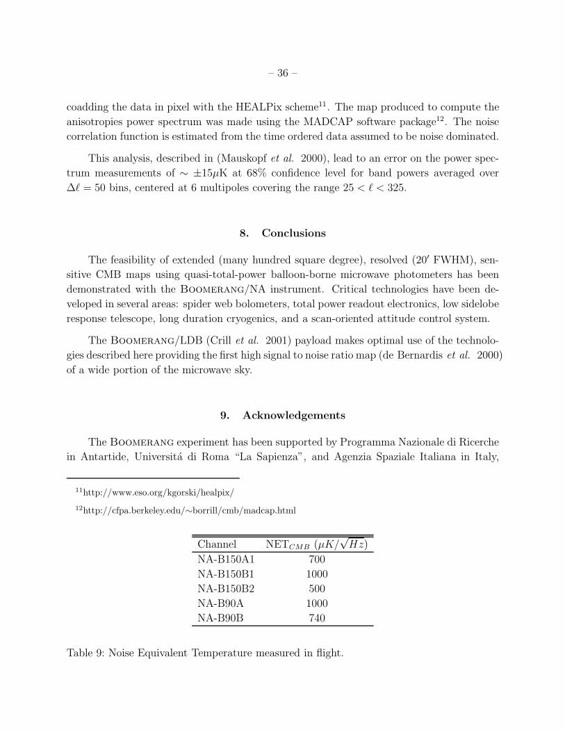
6.4. In flight noise

In flight noise performance is measured computing the power spectrum of the bolometers

signals after de-spiking and deconvolution, avoiding data taken when the gondola inverts the

scanning direction (turnarounds). Noise equivalent temperatures (NET) are calculated using

in flight calibration constants. In flight noise includes bolometer noise, electronics noise,

signal from the atmosphere, radio frequency noise, signal from the Galaxy and signal from

the CMB. Results are in Table 9. Power spectra are reported in Figure 21 for the channels

used in the analysis.

– 34 –

280 300 320 340 360 380 400 420

280

300

320

340

360

380

400

420

B90B B150B2

Mea

sure

d A

zim

uth

of B

97 D

ipol

e (d

egre

es)

Azimuth of COBE Dipole (maximum, degrees)

Fig. 19.— Azimuth of the maximum signal versus azimuth of the expected dipole direction

during fast rotations. The good correlation is a proof that the signal is originated by the

CMB dipole and it is not a local effect.

7. Sensitivity and Data Analysis

The sensitivity of a receiver to fluctuations in sky brightness at different angular scales

can be represented by a window function. The shape of the window function depends on

the details of the measurement. Calculations have been made for the window functions of

different experiments (e.g. (White et al. 1994)) taking into account different beam shapes

and sizes, chopping strategies, signal processing electronics, and data analysis strategies.

Because of the complex chopping strategies employed to obtain stable offsets in these ex-

periments, the window functions are often complicated. Recent experiments attempt to use

specially tailored filters to generate multiple well-defined window functions from a single

chop (Big Plate, MSAM). In addition, upcoming space missions will attempt to make fully

reconstructed maps of diffuse millimeter-wave emission (MAP, Plank). For all of these ex-

periments, the scan strategy is driven by the achievable bandwidth of the detectors which

limits the maximum and minimum scan speed.

– 35 –

0 1 2 3 4 5 6 7

0.98

1.00

1.02

1.04

1.06

1.08

1.10

1.12 B150B2 B90B

Cal

ibra

tion

cons

tant

s (n

orm

aliz

ed t

o #1

0)

Time (hours)

Fig. 20.— Fractional responsivity variations during the flight as measured from the internal

calibrator signals, for both the channels used in the analysis. Starting from the second hour

of flight the variations are less than 10%. The first two hours aren’t used in the data analysis.

In Boomerang we have designed our scan strategy and beam size to utilize the full

bandwidth and sensitivity of our detectors. The scan speed for both flights of Boomerang

is matched to the signal bandwidth of the detectors and the sensitivity to large angular

scales is limited by the stability of the readout electronics and atmospheric fluctuations.

Boomerang can operate in either total power mode with the data from each detector

analyzed independently, or in chopped mode, differencing between symmetric pixels in the

focal plane to remove common mode noise sources. In total power mode, the window function

of each channel is limited only by the beam size and the scan length. In differenced mode,

the window function is determined by the beam size and beam separation in the focal plane.

The data from the BNA flight have been analyzed as a pixellized map with an experi-

mentally determined correlation matrix describing the noise.

Maps of the B150B2 and B90B channels are in Figure 22. The ∼ 25000 pixels maps

are noise dominated. These maps are produced just filtering the Time Ordered Data and

– 36 –

coadding the data in pixel with the HEALPix scheme11. The map produced to compute the

anisotropies power spectrum was made using the MADCAP software package12. The noise

correlation function is estimated from the time ordered data assumed to be noise dominated.

This analysis, described in (Mauskopf et al. 2000), lead to an error on the power spec-

trum measurements of ∼ ±15µK at 68% confidence level for band powers averaged over

∆ℓ = 50 bins, centered at 6 multipoles covering the range 25 < ℓ < 325.

8. Conclusions

The feasibility of extended (many hundred square degree), resolved (20′ FWHM), sen-

sitive CMB maps using quasi-total-power balloon-borne microwave photometers has been

demonstrated with the Boomerang/NA instrument. Critical technologies have been de-

veloped in several areas: spider web bolometers, total power readout electronics, low sidelobe

response telescope, long duration cryogenics, and a scan-oriented attitude control system.

The Boomerang/LDB (Crill et al. 2001) payload makes optimal use of the technolo-

gies described here providing the first high signal to noise ratio map (de Bernardis et al. 2000)

of a wide portion of the microwave sky.

9. Acknowledgements

The Boomerang experiment has been supported by Programma Nazionale di Ricerche

in Antartide, Universita di Roma “La Sapienza”, and Agenzia Spaziale Italiana in Italy,

11http://www.eso.org/kgorski/healpix/

12http://cfpa.berkeley.edu/∼borrill/cmb/madcap.html

Channel NETCMB (µK/√Hz)

NA-B150A1 700

NA-B150B1 1000

NA-B150B2 500

NA-B90A 1000

NA-B90B 740

Table 9: Noise Equivalent Temperature measured in flight.

– 37 –

Fig. 21.— Noise Equivalent Temperature versus frequency for the two channels used in the

analysis of the angular power spectrum of the CMB. At low frequencies 1/f noise dominates.

The rise at high frequencies is due to the bolometer time constants: the receiver looses

sensitivity and the NET is increased after deconvolution. The most interesting frequencies

are around 1.5 Hz where is expected to be the first peak of the anisotropies in the CMB

(with scan speed of 2 deg s−1 at the elevation of 41 deg).

by NSF and NASA in the USA, and by PPARC in the UK. Doe/NERSC provided the

supercomputing facilities. We acknowledge the use of HEALPix.

– 38 –

Fig. 22.— Maps of the measured flight from B150B2 and the B90B channels. Both maps

are smoothed with a 0.5 deg FWHM gaussian in order to increase the signal to noise ratio.

The structures in the maps are only partially concordant, showing that these maps are noise

dominated rather than signal dominated. For better visualization only a portion of the full

map (see coverage in Figure 12) is reported here.

– 39 –

REFERENCES

Alsop, D. C., Inman, C., Lange, A. E., and Wilbanks, T. 1992, Applied Optics, 31, 6610

Bock, J. J. et al. 1996, Proc. 30th ESLAB Symp. Submillimetre and Far-Infrared Space

Instrumentation, ESTEC, Noordwijk, Netherlands, ESA SP-388.

Bond, J. R., Crittenden, R., Davis, R. L., Efstathiou, G., Steinhardt, P. J. 1994, Phys. Rev.

Lett., 72, 13, astro-ph/9309041

Church, S. E., Ganga, K. M., Holzapfel, W. L., Ade, P. A. R., Mauskopf, P. D., Wilbanks,

T. M., and Lange A. E. submitted to Ap. J.

Crill, B. P. et al. 2000, in preparation.

de Bernardis, P., Aquilini, E., Boscaleri, A., De Petris, M., Gervasi, M., Martinis, L., Masi,

S., Natale, V., Palumbo, P., Scaramuzzi, F., Valenziano, L., 1993, Astron. Astrophys.

271, 683

deBernardis, P., DeTroia, G., Miglio, L., 1999, New Astronomy Review, 43, pag. 281-287

deBernardis, P. et al. , 2000, Nature , 404, pag. 955-959, astro-ph/0004404

Devlin, M. J., Clapp, A. C., Gundersen, J. O., Hagmann, C. A., Hristov, V. V., Lange, A.

E., Lim, M. A., Lubin, P. M., Mauskopf, P. D., Richards, P. L., Smoot, G. F., Tanaka,

S. T. 1994, Ap. J. , 433, L57, astro-ph/9404036

Fixsen, D. J., et al. 1994, Ap. J. , 420, 445

Goldin, A. B., et al. 1997, Ap. J. Lett. , 488, 161

Gundersen, J. O., Clapp, A. C., Devlin, M. J., Holmes, W., Fischer, M. L., Meinhold, P. R.,

Lange, A. E., Lubin, P. M., Richards, P. L., et al. 1993, Ap. J. , 413, L1

Halpern, M., Gush, H.P., Wishnow, E., De Cosmo, V., 1986, Applied Optics, 25, 565

Hristov, V. et al. in preparation

Hristov, V. et al. in preparation

Hu, W., Sugiyama, N., Silk, J., 1997, Nature , 386, 37-43, astro-ph/9604166

Kogut, A., and 19 colleagues 1993, Ap. J. , 419, 1

– 40 –

Lee, A. T. et al. , 1999, in ’3K Cosmology’, AIP conference proceedings 476, pag. 224,

Woodbury - New York, Maiani Melchiorri Vittorio Editors

Masi, S., Aquilini, E., Cardoni, P., de Bernardis, P., Martinis, L., Scaramuzzi, F., Sforna.

D., 1998, Cryogenics, 38, N.3

Masi, S., Cardoni, P., de Bernardis, P., Piacentini, F., Raccanelli, A., Scaramuzzi, F., 1999,

Cryogenics, 217-224, N.39

Mather, J. C. et al. 1994, Ap. J. , 420, 439

Mauskopf, P. et al. , 2000, Ap. J. Lett. 536, L59, astro-ph/9911444

Mauskopf P. D., et al., Applied Optics, 36, 765, 1997

Melchiorri, A. et al. , 2000, Ap. J. Lett. 536, L63, astro-ph/9911445

Page, L.A., Cheng, E.S. & Myers, S.S., 1990, Ap. J. 335, L1

Smoot, G. F., et al. 1991, Ap. J. Lett. , 371, L1

Smoot, G., F., et al. 1992, Ap. J. 396, L1

Tanaka, S. T., Clapp, A. C., Devlin, M. J., Figueiredo, N., Gundersen, J. O., Hanany, S.,

Hristov, V. V., Lange, A. E., Lim, M. A., et al. 1996, Ap. J. , 468, L81

Ulich B.L. 1981, AJ, 86, 1619

White, M., Scott, D. & Silk, J. 1994, ARA&A, 32, 319

Wilbanks, T., Devlin, M., Lange, A. E., Sato, S., Beeman, J. W., and Haller, E. E. 1990,

IEEE Transactions on Nuclear Science, 37, 566

This preprint was prepared with the AAS LATEX macros v5.0.