���

Queen’s Economics Department Working Paper No. 1127

Bootstrap Hypothesis Testing

James MacKinnonQueen’s University

Department of EconomicsQueen’s University

94 University AvenueKingston, Ontario, Canada

K7L 3N6

6-2007

Bootstrap Hypothesis Testing

James G. MacKinnon

Department of EconomicsQueen’s University

Kingston, Ontario, CanadaK7L 3N6

jgm@econ.queensu.ca

http://www.econ.queensu.ca/faculty/mackinnon/

Abstract

This paper surveys bootstrap and Monte Carlo methods for testing hypotheses ineconometrics. Several different ways of computing bootstrap P values are discussed,including the double bootstrap and the fast double bootstrap. It is emphasized thatthere are many different procedures for generating bootstrap samples for regressionmodels and other types of model. As an illustration, a simulation experiment exam-ines the performance of several methods of bootstrapping the supF test for structuralchange with an unknown break point.

June 2007; minor revisions, November 2008 and June 2009

This research was supported, in part, by grants from the Social Sciences and HumanitiesResearch Council of Canada. The computations were performed on a Linux cluster fundedby a grant from the Canada Foundation for Innovation, for which I am very grateful toRussell Davidson. I would like to thank John Nankervis and two anonymous referees forhelpful comments. An earlier version was presented at the Conference on Computational andFinancial Econometrics at the University of Geneva in April 2007.

1. Introduction

The basic idea of any sort of hypothesis test is to compare the observed value of a teststatistic, say τ , with the distribution that it would follow if the null hypothesis weretrue. The null is then rejected if τ is sufficiently extreme relative to this distribution.In certain special cases, such as t and F tests on the coefficients of a linear regressionmodel with exogenous regressors and normal errors, this distribution is known, andwe can perform exact tests. In most cases of interest to econometricians, however, thedistribution of the test statistic we use is not known. We therefore have to compare τwith a distribution that is only approximately correct. In consequence, the test mayoverreject or underreject.

Traditionally, the approximations that we use in econometrics have been based onasymptotic theory. But advances in computing have made an alternative approachincreasingly attractive. This approach is to generate a large number of simulatedvalues of the test statistic and compare τ with the empirical distribution function, orEDF, of the simulated ones. Using the term “bootstrap” in a rather broad sense, Iwill refer to this approach as bootstrap testing, although the term simulation-based

testing is more general and might perhaps be more accurate. Bootstrap testing canwork very well indeed in some cases, but it is, in general, neither as easy nor as reliableas practitioners often seem to believe.

Although there is a very large literature on bootstrapping in statistics, a surprisinglysmall proportion of it is devoted to bootstrap testing. Instead, the focus is usually onestimating bootstrap standard errors and constructing bootstrap confidence intervals.Two classic books are Efron and Tibshirani (1993) and Davison and Hinkley (1997).There have been many useful survey papers, including DiCiccio and Efron (1996),MacKinnon (2002), Davison, Hinkley, and Young (2003), and Horowitz (2001, 2003).

The next section discusses the basic ideas of bootstrap testing and its relationshipwith Monte Carlo testing. Section 3 explains what determines how well bootstraptests perform under the null hypothesis. Section 4 discusses double bootstrap andfast double bootstrap tests. Section 5 discusses various bootstrap data generatingprocesses. Section 6 discusses tests of multiple hypotheses. Section 7 presents somesimulation results for a particular case which illustrate how important the choice ofbootstrap DGP can be, and Section 8 concludes.

2. Bootstrap and Monte Carlo Tests

Suppose that τ is the observed value of a test statistic τ , and we wish to perform atest at level α that rejects when τ is in the upper tail. Then the P value, or marginal

significance level, of τ isp(τ) = 1 − F (τ), (1)

where F (τ) is the cumulative distribution function of τ under the null hypothesis. Ifwe knew F (τ), we would simply calculate p(τ) and reject the null whenever p(τ) < α.This is equivalent to rejecting whenever τ exceeds the critical value F1−α(τ), which is

–1–

the 1 − α quantile of F (τ). When we do not know F (τ), which is usually the case, itis common to use an asymptotic approximation to it. This may or may not work well.

An increasingly popular alternative is to perform a bootstrap test. We first gener-ate B bootstrap samples, or simulated data sets, indexed by j. The procedure forgenerating the bootstrap samples is called a bootstrap data generating process, orbootstrap DGP, and there are often a number of choices. Some bootstrap DGPs maybe fully parametric, others may be fully nonparametric, and still others may be partlyparametric; see Section 5. Each bootstrap sample is then used to compute a bootstrap

test statistic, say τ∗

j , most commonly by the same procedure used to calculate τ fromthe real sample. It is strongly recommended that the bootstrap samples should satisfythe null hypothesis, but this is not always possible. When they do not satisfy the null,the τ∗

j cannot be calculated in quite the same way as τ itself.

If we wish to reject when τ is in the upper tail, the bootstrap P value is simply

p∗(τ) = 1 − F ∗(τ) =1

B

B∑

j=1

I(τ∗

j > τ), (2)

where F ∗ denotes the empirical distribution function, or EDF, of the τ∗

j , and I(·)denotes the indicator function, which is equal to 1 when its argument is true and 0otherwise. The inequality would be reversed if we wished to reject when τ is in thelower tail, as with many unit root tests. Thus the bootstrap P value is, in general,simply the proportion of the bootstrap test statistics τ∗

j that are more extreme thanthe observed test statistic τ . In the case of (2), it is in fact the empirical analog of (1).Of course, rejecting the null hypothesis whenever p∗(τ) < α is equivalent to rejectingit whenever τ exceeds the 1 − α quantile of F ∗.

Perhaps surprisingly, this procedure can actually yield an exact test in certain cases.The key requirement is that the test statistic τ should be pivotal, which means thatits distribution does not depend on anything that is unknown. This implies that τ andthe τ∗

j all follow the same distribution if the null is true. In addition, the number ofbootstrap samples B must be such that α(B + 1) is an integer, where α is the level ofthe test. If a bootstrap test satisfies these two conditions, then it is exact. This sort oftest, which was originally proposed in Dwass (1957), is generally called a Monte Carlo

test. For an introduction to Monte Carlo testing, see Dufour and Khalaf (2001).

It is quite easy to see why Monte Carlo tests are exact. Imagine sorting all B + 1 teststatistics. Then rejecting the null whenever p(τ) < α implies rejecting it wheneverτ is one of the largest α(B + 1) statistics. But, if τ and the τ∗

j all follow the samedistribution, this happens with probability precisely α. For example, if B = 999 andα = .01, we reject the null whenever τ is one of the 10 largest test statistics.

Since a Monte Carlo test is exact whenever α(B + 1) is an integer, it is tempting tomake B very small. In principle, it could be as small as 19 for α = .05 and as smallas 99 for α = .01. There are two problems with this, however. The first problem is

–2–

that the smaller is B the less powerful is the test. The loss of power is proportionalto 1/B; see Jockel (1986) and Davidson and MacKinnon (2000).

The second problem is that, when B is small, the results of the test can depend non-trivially on the particular sequence of random numbers used to generate the bootstraptest statistics, and most investigators find this unsatisfactory. Since p∗ is just a fre-quency, the variance of p∗ is p∗(1−p∗)/B. Thus, when p∗ = .05, the standard error ofp∗ is 0.0219 for B = 99, 0.0069 for B = 999, and 0.0022 for B = 9999. This suggeststhat, if computational cost is not a serious concern, it might be dangerous to use avalue of B less than 999, and it would not be unreasonable to use B = 9999.

When computational cost is a concern, but it is not extremely high, it is often possibleto obtain reliable results for a small value of B by using an iterative procedure proposedin Davidson and MacKinnon (2000). The idea is to start with a small value of B, decidewhether the outcome of the test would almost certainly have been the same if B hadbeen ∞, and then increase B if not. This process is then repeated until either anunambiguous result is obtained or it is clear that p∗(τ) is very, very close to α. Forexample, if B = 19, and 5 or more of the τ∗

j are greater than τ , we can safely decidenot to reject at the .05 level, because the probability of obtaining that many values ofτ∗

j larger than τ by chance if p∗ = .05 is very small (it is actually .00024). However, iffewer than 5 of the τ∗

j are greater than τ , we need to generate some more bootstrapsamples and calculate a new P value. Much of the time, especially when the nullhypothesis is true, this procedure stops when B is under 100.

When computational cost is extremely high, two useful procedures have recently beenproposed. Racine and MacKinnon (2007a) proposes a very simple method for per-forming Monte Carlo tests that does not require α(B + 1) to be an integer. However,this procedure may lack power. Racine and MacKinnon (2007b) proposes a more com-plicated method for calculating bootstrap P values that is based on kernel smoothing.The P value depends on the actual values of τ and the τ∗

j , not just on the rank of τ inthe sorted list of all the test statistics. This method does not quite yield exact tests,but it can substantially increase power when B is very small. In some cases, one canreliably reject the null at the .05 level using fewer than 20 bootstrap samples.

Quite a few popular specification tests in econometrics are pivotal if we conditionon the regressors and the distribution of the error terms is assumed to be known.These include any test that just depends on ordinary least squares residuals and onthe matrix of regressors and that does not depend on the variance of the error terms.Examples include the Durbin-Watson test and several other tests for serial correla-tion, as well as popular tests for heteroskedasticity, skewness, and kurtosis. Tests forheteroskedasticity will be discussed further in the next section.

It is very easy to perform this sort of Monte Carlo test. After we calculate τ from theresidual n--vector u and, possibly, the regressor matrix X, we generate B bootstrapsamples. We can do this by generating B vectors of length n from the standard normaldistribution, or possibly from some other assumed distribution, and regressing each ofthem on X so as to obtain B vectors of bootstrap residuals u∗

j . We then calculate each

–3–

of the bootstrap statistics τ∗

j from u∗

j in the same way that we calculated τ from u.Provided we have chosen B correctly, the bootstrap P value (2) will then provide uswith an exact test.

Even when τ is not pivotal, using the bootstrap to compute a P value like (2) isasymptotically valid. Moreover, this type of bootstrap testing can in many cases yieldmore accurate results than using an asymptotic distribution to compute a P value.This subject will be discussed in the next section.

When we wish to perform a two-tailed test, we cannot use equation (2) to computea bootstrap P value. If we are willing to assume that τ is symmetrically distributedaround zero, we can use the symmetric bootstrap P value

p∗s (τ) =1

B

B∑

j=1

I(|τ∗

j | > |τ |), (3)

which effectively converts a two-tailed test into a one-tailed test. If we are not willing tomake this assumption, which can be seriously false for t statistics based on parameterestimates that are biased, we can instead use the equal-tail bootstrap P value

p∗et(τ) = 2 min

(1

B

B∑

j=1

I(τ∗

j ≤ τ),1

B

B∑

j=1

I(τ∗

j > τ)

). (4)

Here we actually perform two tests, one against values in the lower tail of the distri-bution and the other against values in the upper tail. The factor of 2 is necessary totake account of this. Without it, p∗et would lie between 0 and 0.5. If the mean of theτ∗

j is far from zero, p∗s and p∗et may be very different, and tests based on them mayhave very different properties under both null and alternative hypotheses.

Of course, equation (3) can only apply to test statistics that can take either sign,such as t statistics. For test statistics that are always positive, such as ones that areasymptotically chi-squared, only equation (2) is usually applicable. But we could use(4) if we wanted to reject for small values of the test statistic as well as for large ones.

Equations (2), (3), and (4) imply that the results of a bootstrap test are invariantto monotonically increasing transformations of the test statistic. Applying the sametransformation to all the test statistics does not affect the rank of τ in the sortedlist of τ and the τ∗

j , and therefore it does not affect the bootstrap P value. One ofthe implications of this result is that, for linear and nonlinear regression models, abootstrap F test and a bootstrap likelihood ratio test based on the same bootstrapDGP must yield the same outcome.

3. Finite-Sample Properties of Bootstrap Tests

Even when B is infinite, bootstrap tests will generally not be exact when τ is notpivotal. Their lack of exactness arises from the difference between the true distribution

–4–

characterized by the CDF F (τ) and the bootstrap distribution characterized by theCDF F ∗(τ). When more than one sort of bootstrap DGP can be used, we shouldalways use the one that makes F ∗(τ) as close as possible to F (τ) in the neighborhoodof the critical value F1−α(τ). Unfortunately, this is easier said than done. Either verysophisticated econometric theory or extensive simulation experiments may be neededto determine which of several bootstrap DGPs leads to the most reliable tests.

A very important result, which may be found in Beran (1988), shows that, when atest statistic is asymptotically pivotal, bootstrapping yields what is generally calledan asymptotic refinement. A test statistic is asymptotically pivotal if its asymptoticdistribution does not depend on anything that is unknown. If a test statistic has aconventional asymptotic distribution such as standard normal or chi-squared, then itmust be asymptotically pivotal. But a test statistic can be asymptotically pivotalwithout having a known asymptotic distribution. In this context, what is meant byan asymptotic refinement is that the error in rejection probability, or ERP, of thebootstrap test is of a lower order in the sample size n than the ERP of an asymptotictest based on the same test statistic.

A serious treatment of asymptotic refinements is well beyond the scope of this paper.Rigorous discussions are generally based on Edgeworth expansions of the distributionsof test statistics; see Beran (1988) and Hall (1992). Davidson and MacKinnon (1999)take a different approach based on what they call the rejection probability function,or RPF, which relates the probability that a test will reject the null to one or morenuisance parameters. Strictly speaking, this approach applies only to parametric boot-strap tests, but it helps to illuminate other cases as well.

Consider the case in which the DGP depends on a single nuisance parameter. If theRPF is flat, as it must be when a test statistic is pivotal, then a parametric bootstraptest will be exact, because the value of the nuisance parameter does not matter. Whenthe RPF is not flat, as is commonly the case, a bootstrap test will generally not beexact, because the estimated parameter of the bootstrap DGP will differ from the(unknown) parameter of the true DGP. How well a bootstrap test performs in such acase depends on the slope and curvature of the RPF and the bias and precision of theestimated nuisance parameter.

Although the actual behavior of bootstrap tests in simulation experiments does notaccord well with theory in every case, the literature on the finite-sample properties ofbootstrap tests has produced several theoretical results of note:

• When a test statistic is asymptotically pivotal, bootstrapping it will generally yielda test with an ERP of lower order in the sample size than that of an asymptotictest based on the same statistic.

• When a test statistic is not asymptotically pivotal, bootstrapping it will generallyyield an asymptotically valid test, but the ERP of the bootstrap test will not beof lower order in the sample size than that of an asymptotic test.

–5–

• In many cases, the reduction in ERP due to bootstrapping is O(n−1/2) for one-tailed tests and O(n−1) for two-tailed tests that assume symmetry around theorigin. Note that, when a test statistic is asymptotically chi-squared, a test thatrejects when the statistic is in the upper tail has the properties of a two-tailed testfrom the point of view of this theory. In contrast, a test based on the equal-tailP value (4) has the properties of a one-tailed test.

• To minimize the Type I errors committed by bootstrap tests, we should attemptto estimate the bootstrap DGP as efficiently as possible. This generally meansimposing the null hypothesis whenever it is possible to do so.

In general, bootstrap tests can be expected to perform well under the null wheneverthe bootstrap DGP provides a good approximation to those aspects of the true DGPto which the distribution of the test statistic is sensitive. Since different test statisticsmay be sensitive to different features of the DGP, it is quite possible that a particularbootstrap DGP may work well for some tests and poorly for others.

It is not always easy to impose the null hypothesis on a bootstrap DGP without alsoimposing parametric assumptions that the investigator may not be comfortable with.Various partly or wholly nonparametric bootstrap DGPs, some of which impose thenull and some of which do not, are discussed in Section 5. Martin (2007) discusseshow to impose the null in a nonparametric way in certain cases of interest.

Although there is always a modest loss of power due to bootstrapping when B issmall, bootstrapping when B is large generally has little effect on power. Comparingthe power of tests that do not have the correct size is fraught with difficulty; seeDavidson and MacKinnon (2006a). It is shown in that paper that, if bootstrap andasymptotic tests based on the same test statistic are size-corrected in a sensible way,then any difference in power should be modest.

Since Monte Carlo tests are exact, and bootstrap tests are generally not exact, it mayseem attractive to use the former whenever possible. The problem is that, in orderto do so, it is generally necessary to make strong distributional assumptions. Forconcreteness, consider tests for heteroskedasticity. Dufour et al. (2004) show that manypopular test statistics for heteroskedasticity in the linear regression model y = Xβ+u

are pivotal when the regressors are treated as fixed and the distribution of the errorterms is known up to a scale factor. These statistics all have the form τ(Z, MXu).That is, they simply depend on a matrix Z of regressors that is treated as fixed andon the residual vector MXu, where the projection matrix MX yields residuals from aregression on X. Moreover, they are invariant to σ2, the variance of the error terms.

One particularly popular procedure, proposed in Koenker (1981), involves taking thevector of residuals MXy, squaring each element, regressing the squared residuals ona constant and the matrix Z, and then calculating the usual F statistic for all slopecoefficients to be zero. The Koenker procedure is asymptotically invariant to thedistribution of the error terms. It was originally proposed as a modification to the LMtest of Breusch and Pagan (1979), which is asymptotically valid only when the errorterms are normally distributed.

–6–

Performing a Monte Carlo test for heteroskedasticity simply involves drawing B errorvectors u∗

j from an assumed distribution, using each of them to calculate a bootstrapstatistic τ(Z, MXu∗

j ), and then calculating a P value by (2). But what if the assumeddistribution is incorrect? As Godfrey, Orme, and Santos Silva (2005) show, when thedistribution from which the u∗

j are drawn differs from the true distribution of u, MonteCarlo tests for heteroskedasticity can be seriously misleading. In particular, MonteCarlo versions of Breusch-Pagan tests can overreject or underreject quite severely insamples of any size, while Monte Carlo versions of Koenker tests can suffer from modestsize distortions when the sample size is small. In contrast, nonparametric bootstraptests in which the u∗

j are obtained by resampling residuals (this sort of bootstrap DGPwill be discussed in Section 5) always yield valid results for large samples and generallyperform reasonably well even in small samples.

None of these results is at all surprising. In order to obtain valid results in largesamples, we either need to use a test statistic, such as the F statistic of Koenker (1981),that is asymptotically invariant to the distribution of the error terms, or we need touse a bootstrap DGP that adapts itself asymptotically to the distribution of the errorterms, or preferably both. Using a Monte Carlo test based on the wrong distributionalassumption together with a test statistic that is not asymptotically invariant to thedistribution of the error terms is a recipe for disaster.

Another way to get around this sort of problem, instead of using a nonparametricbootstrap, is proposed in Dufour (2006). This paper introduces maximized Monte

Carlo tests. In principle, these can be applied to any sort of test statistic where thenull distribution depends on one or more nuisance parameters. The idea is to performa (possibly very large) number of simulation experiments, each for a different set ofnuisance parameters. Using some sort of numerical search algorithm, the investigatorsearches over the nuisance parameter(s) in an effort to maximize the bootstrap Pvalue. The null hypothesis is rejected only if the maximized P value is less thanthe predetermined level of the test. In the context of testing for heteroskedasticity,it is necessary to search over a set of possible error distributions. An application ofmaximized Monte Carlo tests to financial economics may be found in Beaulieu, Dufour,and Khalaf (2007).

The idea of maximized Monte Carlo tests is elegant and ingenious, but these tests canbe very computationally demanding. Moreover, their actual rejection frequency maybe very much less than the level of the test, and they may in consequence be severelylacking in power. This can happen when the RPF is strongly dependent on the value(s)of one or more nuisance parameters, and there exist parameter values (perhaps far awayfrom the ones that actually generated the data) for which the rejection probabilityunder the null is very high. The maximized Monte Carlo procedure will then assigna much larger P value than the one that would have been obtained if the true, butunknown, values of the nuisance parameters had been used.

–7–

4. Double Bootstrap and Fast Double Bootstrap Tests

It seems plausible that, if bootstrapping a test statistic leads to an asymptotic refine-ment, then bootstrapping a quantity that has already been bootstrapped will lead to afurther refinement. This is the basic idea of the iterated bootstrap, of which a specialcase is the double bootstrap, proposed in Beran (1987, 1988).

There are at least two quite different types of double bootstrap test. The first typepotentially arises whenever we do not have an asymptotically pivotal test statistic tostart with. Suppose, for example, that we obtain a vector of parameter estimates θ

but no associated covariance matrix Var(θ), either because it is impossible to estimateVar(θ) at all or because it is impossible to obtain a reasonably accurate estimate. Wecan always use the bootstrap to estimate Var(θ). If θ∗

j denotes the estimate from thej th bootstrap sample, and θ∗ denotes the average of the bootstrap estimates, then

Var(θ) ≡ 1

B

B∑

j=1

(θ∗

j − θ∗)(θ∗

j − θ∗)⊤

provides a reasonable way to estimate Var(θ). Note that whatever bootstrap DGP isused here should not impose any restrictions on θ.

We can easily construct a variety of Wald statistics using θ and Var(θ). The simplestwould just be an asymptotic t statistic for some element of θ to equal a particularvalue. Creating a t statistic from a parameter estimate, or a Wald statistic from avector of parameter estimates, is sometimes called prepivoting, because it turns aquantity that is not asymptotically pivotal into one that is.

Even though test statistics of this sort are asymptotically pivotal, their asymptoticdistributions may not provide good approximations in finite samples. Thus it seemsnatural to bootstrap them. Doing so is conceptually easy but computationally costly.The procedure works as follows:

1. Obtain the estimates θ.

2. Generate B2 bootstrap samples from a bootstrap DGP that does not impose anyrestrictions, and use them to estimate Var(θ).

3. Calculate whatever test statistic τ ≡ τ(θ, Var(θ)

)is of interest.

4. Generate B1 bootstrap samples using a bootstrap DGP that imposes whateverrestrictions are to be tested. Use each of them to calculate θ∗

j .

5. For each of the B1 bootstrap samples, perform steps 2 and 3 exactly as before.This yields B1 bootstrap test statistics τ∗

j ≡ τ(θ∗

j , Var(θ∗

j )).

6. Calculate the bootstrap P value for τ using whichever of the formulas (2), (3), or(4) is appropriate, with B1 playing the role of B.

This procedure is conceptually simple, and, so long as the procedure for computingθ is reliable, it should be straightforward to implement. The major problem is com-putational cost, which can be formidable, because we need to obtain no less than

–8–

(B1 + 1)(B2 + 1) estimates of θ. For example, if B1 = 999 and B2 = 500, we needto obtain 501,000 sets of estimates. It may therefore be attractive to utilize eitherthe method of Davidson and MacKinnon (2000) or the one of Racine and MacKinnon(2007b), or both together, because they can allow B1 to be quite small.

The second type of double bootstrap test arises when we do have an asymptoticallypivotal test statistic τ to start with. It works as follows:

1. Obtain the test statistic τ and whatever estimates are needed to generate boot-strap samples that satisfy the null hypothesis.

2. Generate B1 bootstrap samples that satisfy the null, and use each of them tocompute a bootstrap statistic τ∗

j for j = 1, . . . , B1.

3. Use τ and the τ∗

j to calculate the first-level bootstrap P value p∗(τ) according to,for concreteness, equation (2).

4. For each of the B1 first-level bootstrap samples, generate B2 second-level boot-strap samples, and use each of them to compute a second-level bootstrap teststatistic τ∗∗

jl for l = 1, . . . , B2.

5. For each of the B1 first-level bootstrap samples, compute the second-level boot-strap P value

p∗∗j =1

B2

B2∑

l=1

I(τ∗∗

jl > τ∗

j ).

Observe that this formula is very similar to equation (2), but we are comparingτ∗

j with the τ∗∗

jl instead of comparing τ with the τ∗

j .

6. Compute the double-bootstrap P value as the proportion of the p∗∗j that aresmaller (i.e., more extreme) than p∗(τ):

p∗∗(τ) =1

B1

B1∑

j=1

I(p∗∗j < p∗(τ)

). (5)

In order to avoid the possibility that p∗∗j = p∗(τ), which would make the strictinequality here problematical, it is desirable that B2 6= B1.

This type of double bootstrap simply treats the single bootstrap P value as a teststatistic and bootstraps it. Observe that (5) is just like (2), but with the inequalityreversed. Like the first type of double bootstrap, this one is computationally demand-ing, as we need to calculate 1 + B1 + B1B2 test statistics, and it may therefore beattractive to employ methods that allow B1 and/or B2 to be small.

The computational cost of performing this type of double bootstrap procedure canbe substantially reduced by utilizing one or more ingenious stopping rules proposed inNankervis (2005). The idea of these stopping rules is to avoid unnecessarily calculatingsecond-level bootstrap test statistics that do not affect the decision on whether or notto reject the null hypothesis.

–9–

The asymptotic refinement that we can expect from the second type of double boot-strap test is greater than we can expect from the first type. For the first type, theERP will normally be of the same order in the sample size as the ERP of an ordinary(single) bootstrap test. For the second type, it will normally be of lower order. Ofcourse, this does not imply that double bootstrap tests of the second type will alwayswork better than double bootstrap tests of the first type.

Davidson and MacKinnon (2007) proposes a procedure for computing fast double

bootstrap, or FDB, P values for asymptotically pivotal test statistics. It is muchless computationally demanding than performing a true double bootstrap, even if theprocedures of Nankervis (2005) are employed, because there is just one second-levelbootstrap sample for each first-level one, instead of B2 of them. Steps 1, 2, and 3 ofthe procedure just given are unchanged, except that B replaces B1. Steps 4, 5, and 6are replaced by the following ones:

4. For each of the B bootstrap samples, generate a single dataset using a second-levelbootstrap sample, and use it to compute a second-level test statistic τ∗∗

j .

5. Calculate the 1 − p∗ quantile of the τ∗∗

j , denoted by Q∗∗

B (1 − p∗) and definedimplicitly by the equation

1

B

B∑

j=1

I(τ∗∗

j < Q∗∗

B

(1 − p∗(τ)

))= 1 − p∗(τ). (6)

Of course, for finite B, there will be a range of values of Q∗∗

B that satisfy (6), andwe must choose one of them somewhat arbitrarily.

6. Calculate the FDB P value as

p∗∗F (τ) =1

B

B∑

j=1

I(τ∗

j > Q∗∗

B (1 − p∗(τ)))

.

Thus, instead of seeing how often the bootstrap test statistics are more extremethan the actual test statistic, we see how often they are more extreme than the1 − p∗ quantile of the τ∗∗

j .

The great advantage of this procedure is that it involves the calculation of just 2B +1test statistics, although B should be reasonably large to avoid size distortions on theorder of 1/B. However, for the FDB to be asymptotically valid, τ must be asymp-totically independent of the bootstrap DGP. This is a reasonable assumption for theparametric bootstrap when the parameters of the bootstrap DGP are estimated underthe null hypothesis, because a great many test statistics are asymptotically indepen-dent of all parameter estimates under the null; see Davidson and MacKinnon (1999).1

1 For the linear regression model y = X1β1 + X2β2 + u with normal errors, it is easyto show that the F statistic for β2 = 0 is independent of the restricted estimates β1,because the latter depend on the projection of y onto the subspace spanned by thecolumns of X1, and the former depends on its orthogonal complement. For moregeneral types of model, the same sort of independence holds, but only asymptotically.

–10–

The assumption makes sense in a number of other cases as well, including the residualand wild bootstraps when they use parameter estimates under the null.

There is no guarantee that double bootstrap tests will always work well. Experiencesuggests that, if the improvement in ERP from using a single-level bootstrap test ismodest, then the further gain from using either a double bootstrap test of the secondtype or an FDB test is likely to be even more modest.

5. Bootstrap Data Generating Processes

From the discussion in Section 3, it is evident that the choice of bootstrap DGPis absolutely critical. Just what choices are available depend on the model beingestimated and on the assumptions that the investigator is willing to make.

At the heart of many bootstrap DGPs is the idea of resampling, which was the keyfeature of the earliest bootstrap methods proposed in Efron (1979, 1982). Supposewe are interested in some quantity θ(y), where y is an n--vector of data with typicalelement yt. What is meant by resampling is that each element of every bootstrapsample y∗

j is drawn randomly from the EDF of the yt, which assigns probability 1/nto each of the yt. Thus each element of every bootstrap sample can take on n possiblevalues, namely, the values of the yt, each with probability 1/n. Each bootstrap sampletherefore contains some of the yt just once, some of them more than once, and someof them not at all.

Resampling is conceptually simple and computationally efficient. It works in theory,at least asymptotically, because the EDF consistently estimates the distribution ofthe yt. For regression models, and other models that involve averaging, it often worksvery well in practice. However, in certain respects, the bootstrap samples y∗

j differfundamentally from the original sample y. For example, the largest element of y∗

j cannever exceed the largest element of y and will be less than it nearly 37% of the time.Thus resampling is likely to yield very misleading results if we are primarily interestedin the tails of a distribution.

Bootstrap samples based on resampling are less diverse than the original sample. Whenthe yt are drawn from a continuous distribution, the n elements of y are all different.But the n elements of each bootstrap sample inevitably include a number of duplicates,because the probability that any element of the original sample will not appear in aparticular bootstrap sample approaches 1/e = 0.3679 as n → ∞. This can causebootstrap DGPs based on resampling to yield invalid inferences, even asymptotically.An important example is discussed in Abadie and Imbens (2006), which shows thatcertain bootstrap methods based on resampling are invalid for matching estimators.

Resampling can be used in a variety of ways. One of the most general and widelyused bootstrap DGPs is the pairs bootstrap, or pairwise bootstrap, which dates backto Freedman (1981, 1984). The idea is simply to resample the data, keeping thedependent and independent variables together in pairs. In the context of the linearregression model y = Xβ + u, this means forming the matrix [y X] with typical row

–11–

[yt Xt] and resampling the rows of this matrix. Each observation of a bootstrapsample is [y∗

t X∗t ], a randomly chosen row of [y X]. This method implicitly assumes

that each observation [yt Xt] is an independent random drawing from a multivariatedistribution, which may or may not be a reasonable assumption.

The pairs bootstrap can be applied to a very wide range of models, not merely regres-sion models. It is most natural to use it with cross-section data, but it is often usedwith time-series data as well. When the regressors include lagged dependent variables,we simply treat them the same way as any other column of X. The pairs bootstrapdoes not require that the error terms be homoskedastic. Indeed, error terms do notexplicitly appear in the bootstrap DGP at all. However, a serious drawback of thismethod is that it does not condition on X. Instead, each bootstrap sample has adifferent X∗ matrix. This can lead to misleading inferences in finite samples when thedistribution of a test statistic depends strongly on X.

In the context of bootstrap testing, the pairs bootstrap is somewhat unsatisfactory.Because it is completely nonparametric, the bootstrap DGP does not impose anyrestrictions on the parameters of the model. If we are testing such restrictions, asopposed to estimating covariance matrices or standard errors, we need to modify thebootstrap test statistic so that it is testing something which is true in the bootstrapDGP. Suppose the actual test statistic takes the form of a t statistic for the hypothesisthat β = β0:

τ =β − β0

s(β).

Here β is the unrestricted estimate of the parameter β that is being tested, and s(β) isits standard error. The bootstrap test statistic cannot test the hypothesis that β = β0,because that hypothesis is not true for the bootstrap DGP. Instead, we must use thebootstrap test statistic

τ∗

j =β∗

j − β

s(β∗

j ), (7)

where β∗

j is the estimate of β from the j th bootstrap sample, and s(β∗

j ) is its standarderror, calculated by whatever procedure was employed to calculate s(β) using theactual sample. Since the estimate of β from the bootstrap samples should, on average,be equal to β, at least asymptotically, the null hypothesis tested by τ∗

j is “true” forthe pairs bootstrap DGP.

As an aside, when s(β) is difficult to compute, it is very tempting to replace s(β∗

j )in (7) by s(β). This temptation should be resisted at all costs. If we were to usethe same standard error to compute both τ and τ∗

j , then we would effectively beusing the nonpivotal quantity β − β0 as a test statistic. Bootstrapping it would beasymptotically valid, but it would offer no asymptotic refinement. We can always usethe bootstrap to compute s(β) and the s(β∗

j ), which will lead to the first type of doublebootstrap test discussed in the previous section.

–12–

In the case of a restriction like β = β0, it is easy to modify the bootstrap test statistic,as in (7), so that bootstrap testing yields valid results. But this may not be so easyto do when there are several restrictions and some of them are nonlinear. Great caremust be taken when using the pairs bootstrap in such cases.

Many simulation results suggest that the pairs bootstrap is never the procedure ofchoice for regression models. Consider the nonlinear regression model

yt = xt(β) + ut, ut ∼ IID(0, σ2), (8)

where xt(β) is a regression function, in general nonlinear in the parameter vector β,that implicitly depends on exogenous and predetermined variables. It is assumedeither that the sample consists of cross-section data or that the regressand and allregressors are stationary. Note that the error terms ut are assumed to be independentand identically distributed.

A good way to bootstrap this sort of model is to use the residual bootstrap. Thefirst step is to estimate (8) under the null hypothesis, obtaining parameter estimatesβ and residuals ut. If the model (8) does not have a constant term or the equivalent,then the residuals may not have mean zero, and they should be recentered. Unless thetest statistic to be bootstrapped is invariant to the variance of the error terms, it isadvisable to rescale the residuals so that they have the correct variance. The simplesttype of rescaled residual is

ut ≡(

n

n − k1

)1/2

ut, (9)

where k1 is the number of parameters estimated under the null hypothesis. The firstfactor here is the inverse of the square root of the factor by which 1/n times the sumof squared residuals underestimates σ2. A somewhat more complicated method usesthe diagonals of the hat matrix, that is, X(X⊤X)−1X⊤, to rescale each residual by adifferent factor. It may work a bit better than (9) when some observations have highleverage. Note that this method is a bit more complicated than the analogous onefor the wild bootstrap that is described below, because we need to ensure that therescaled residuals have mean zero; see Davidson and MacKinnon (2006b).

The residual bootstrap DGP may be written as

y∗

t = xt(β) + u∗

t , u∗

t ∼ EDF(ut). (10)

In other words, we evaluate the regression function at the restricted estimates and thenresample from the rescaled residuals. There might be a slight advantage in terms ofpower if we were to use unrestricted rather than restricted residuals in (10). This wouldinvolve estimating the unrestricted model to obtain residuals ut and then replacing ut

by ut and k1 by k in (9). What is important is that we use β rather than β. Doingso allows us to compute the bootstrap test statistics in exactly the same way as theactual one. Moreover, since β will, in most cases, be more precisely estimated than β,

–13–

the bootstrap DGP (10) will more closely approximate the true DGP than it would ifwe used β.

When xt(β) includes lagged values of the dependent variable, the residual bootstrapshould be modified so that the y∗

t are generated recursively. For example, if therestricted model were yt = β1 + β2zt + β3yt−1 + ut, the bootstrap DGP would be

y∗

t = β1 + β2zt + β3y∗

t−1 + u∗

t , u∗

t ∼ EDF(ut). (11)

In most cases, the observed pre-sample value(s) of yt are used to start the recursion.It is important that the bootstrap DGP should be stationary, which in this case meansthat |β3| < 1. If this condition is not satisfied naturally, it should be imposed on thebootstrap DGP.

The validity of the residual bootstrap depends on the strong assumption that theerror terms are independent and identically distributed. We cannot use it when theyare actually heteroskedastic. If the form of the heteroskedasticity is known, we caneasily modify the residual bootstrap by introducing a skedastic function, estimatingit, using feasible weighted least squares (linear or nonlinear), and then resamplingfrom standardized residuals. But if the form of the heteroskedasticity is unknown, thebest method that is currently available, at least for tests on β, seems to be the wild

bootstrap, which was originally proposed in Wu (1986).

For a restricted version of a model like (8), with independent but possibly heteroskedas-tic error terms, the wild bootstrap DGP is

y∗

t = xt(β) + f(ut)v∗

t ,

where f(ut) is a transformation of the tth residual ut, and v∗

t is a random variable withmean 0 and variance 1. One possible choice for f(ut) is just ut, but a better choice is

f(ut) =ut

(1 − ht)1/2, (12)

where ht is the tth diagonal of the “hat matrix” that was defined just after (9). Whenthe f(ut) are defined by (12), they would have constant variance if the error termswere homoskedastic.

There are various ways to specify the distribution of the v∗t . The simplest, but not the

most popular, is the Rademacher distribution,

v∗

t = 1 with probability 1

2; v∗

t = −1 with probability 1

2. (13)

Thus each bootstrap error term can take on only two possible values. Davidson andFlachaire (2008) have shown that wild bootstrap tests based on (13) usually performbetter than wild bootstrap tests which use other distributions when the conditionaldistribution of the error terms is approximately symmetric. When this distribution is

–14–

sufficiently asymmetric, however, it may be better to use another two-point distribu-tion, which is the one that is most commonly used in practice:

v∗

t =

{−(

√5 − 1)/2 with probability (

√5 + 1)/(2

√5);

(√

5 + 1)/2 with probability (√

5 − 1)/(2√

5).

In either case, since the expectation of the square of ut is approximately the varianceof ut, the wild bootstrap error terms will, on average, have about the same variance asthe ut. In many cases, this seems to be enough for the wild bootstrap DGP to mimicthe essential features of the true DGP.

Although it is most natural to use the wild bootstrap with cross-section data, it canalso be used with at least some types of time-series model, provided the error termsare uncorrelated. See Goncalves and Kilian (2004). The wild bootstrap can also beused with clustered data. In this case, the entire vector of residuals for each clusteris multiplied by v∗

t for each bootstrap sample so as to preserve any within-clusterrelationships among the error terms. See Cameron, Gelbach, and Miller (2008).

Bootstrap methods may be particularly useful in the case of multivariate regressionmodels, because standard asymptotic tests often overreject severely; see Stewart (1997)and Dufour and Khalaf (2002). When there are g dependent variables, a multivariatenonlinear regression model can be written, using notation similar to that of (8), as

yti = xti(β) + uti, t = 1, . . . , n, i = 1, . . . , g. (14)

If we arrange the yti, xti, and uti into g--vectors yt, xt, and ut, respectively, the model(14) can be written more compactly as

yt = xt(β) + ut, E(utut⊤) = Σ. (15)

Here the conventional assumption that the error terms are correlated across equations,but homoskedastic and serially uncorrelated, is made explicit. The model (15) istypically estimated by either feasible GLS or maximum likelihood. Doing so under thenull hypothesis yields parameter estimates β and residuals ut.

The residual bootstrap DGP for the model (15) is simply

y∗

t = xt(β) + u∗

t , u∗

t ∼ EDF(ut), (16)

which is analogous to (10). We evaluate the regression functions at the restrictedestimates β and resample from vectors of residuals, as in the pairs bootstrap. Thisresampling preserves the joint empirical distribution of the residuals, and in particularthe correlations among them, without imposing any distributional assumptions. Thisapproach is simpler and less restrictive than drawing the u∗

t from a multivariate normaldistribution with covariance matrix estimated from the ut, which is a procedure thatis also sometimes used. Of course, we may wish to impose the normality assumption

–15–

since, in some cases, doing so makes it possible to perform Monte Carlo tests onmultivariate linear regression models; see Dufour and Khalaf (2002). Alternatively, ifwe wished to allow for heteroskedasticity, we could use a wild bootstrap.

A particularly important type of multivariate regression model is the simultaneous

equations model. Often, we are only interested in one equation from such a model,and it is estimated by generalized instrumental variables (also called two-stage leastsquares). A model with one structural equation and one or more reduced form equa-tions may be written as

y = Zβ1 + Yβ2 + u (17)

Y = WΠ + V . (18)

Here y is an n× 1 vector of the endogenous variable of interest, Y is an n× g matrixof other endogenous variables, Z is an n × k matrix of exogenous variables, and W

is an n × l matrix of instruments, which must include all the exogenous variables. Infinite samples, inferences about β1 and β2 based on asymptotic theory can be veryunreliable, so it is natural to think about bootstrapping.

However, bootstrapping this model requires some effort. Even if we are only interestedin the structural equation (17), the bootstrap DGP must generate both y∗ and Y ∗.We could just use the pairs bootstrap (Freedman, 1984), but it often does not workvery well. In order to use the residual bootstrap, we need estimates of β1, β2, andΠ, as well as a way to generate the bootstrap error terms u∗ and V ∗. It is naturalto use 2SLS estimates of β1 and β2 from (17) under the null hypothesis, along withOLS estimates of Π from (18). The bootstrap error terms may then be obtained byresampling from the residual vectors [ut, Vt], as in (16).

Although the residual bootstrap DGP just described is asymptotically valid and gen-erally provides less unreliable inferences than using asymptotic tests, it often does notwork very well. But its finite-sample properties can be greatly improved if we use OLSestimates Π ′ from the system of regressions

Y = WΠ + uδ⊤ + residuals (19)

rather than the usual OLS estimates Π from (18). In (19), u is the vector of 2SLSresiduals from estimation of (17) under the null hypothesis, and δ is a g--vector ofcoefficients to be estimated. We also use V ′ ≡ Y − WΠ ′ instead of V when weresample the bootstrap error terms.

It was shown in Davidson and MacKinnon (2008) that, in the case in which thereis just one endogenous right-hand-side variable, t statistics for β2 = 0 are far morereliable when the bootstrap DGP uses Π ′ and V ′ than when it uses Π and V . Thisis especially true when the instruments are weak, which is when asymptotic tests tendto be seriously unreliable. A wild bootstrap variant of this procedure, which allowsfor heteroskedasticity of unknown form, was proposed in Davidson and MacKinnon(2009).

–16–

Any sort of resampling requires independence. Either the data must be treated asindependent drawings from a multivariate distribution, as in the pairs bootstrap, orthe error terms must be treated as independent drawings from either univariate ormultivariate distributions. In neither case can serial dependence be accommodated.Several bootstrap methods that do allow for serial dependence have been proposed,however. Surveys of these methods include Buhlmann (2002), Horowitz (2003), Politis(2003), and Hardle, Horowitz, and Kreiss (2003).

One way to generalize the residual bootstrap to allow for serial correlation is to usewhat is called the sieve bootstrap, which assumes that the error terms follow anunknown, stationary process with homoskedastic innovations. The sieve bootstrap,which was given its name in Buhlmann (1997), attempts to approximate this stationaryprocess, generally by using an AR(p) process, with p chosen either by some sort ofmodel selection criterion or by sequential testing. One could also use MA or ARMAprocesses, and this appears to be preferable in some cases; see Richard (2007).

After estimating the regression model, say (8), under the null hypothesis, we retainthe residuals and use them to select the preferred AR(p) process and estimate itscoefficients, making sure that it is stationary. Of course, this two-step procedurewould not be valid if (8) were a dynamic model. Then the bootstrap DGP is

u∗

t =

p∑

i=1

ρiu∗

t−i + ε∗t , t = −m, . . . , 0, 1, . . . , n,

y∗

t = xt(β) + u∗

t , t = 1, . . . , n,

where the ρi are the estimated parameters, and the ε∗t are resampled from the (possiblyrescaled) residuals of the AR(p) process. Here m is an arbitrary number, such as 100,chosen so that the process can be allowed to run for some time before the sampleperiod starts. We set the initial values of u∗

t−i to zero and discard the u∗

t for t < 1.

The sieve bootstrap is somewhat restrictive, because it rules out GARCH models andother forms of conditional heteroskedasticity. Nevertheless, it is quite popular. It hasrecently been applied to unit root testing in Park (2003) and Chang and Park (2003),and it seems to work quite well in many cases.

Another approach that is more in the spirit of resampling and imposes fewer assump-tions is the block bootstrap, originally proposed in Kunsch (1989). The idea is todivide the quantities that are being resampled into blocks of b consecutive observa-tions. These quantities may be either rescaled residuals or [y, X] pairs. The blocks,which may be either overlapping or nonoverlapping and may be either fixed or vari-able in length, are then resampled. Theoretical results due to Lahiri (1999) suggestthat the best approach is to use overlapping blocks of fixed length. This is called themoving-block bootstrap.

For the moving-block bootstrap, there are n − b + 1 blocks. The first contains obser-vations 1 through b, the second contains observations 2 through b + 1, and the last

–17–

contains observations n− b +1 through n. Each bootstrap sample is then constructedby resampling from these overlapping blocks. Unless n/b is an integer, one or more ofthe blocks will have to be truncated to form a sample of length n.

A variant of the moving-block bootstrap for dynamic models is the block-of-blocks

bootstrap (Politis and Romano, 1992), which is analogous to the pairs bootstrap.Consider the dynamic regression model

yt = Xtβ + γyt−1 + ut, ut ∼ IID(0, σ2).

If we define Zt as [yt, yt−1, Xt], then we can construct n− b + 1 overlapping blocks as

Z1 . . .Zb; Z2 . . .Zb+1; . . . . . . ; Zn−b+1 . . .Zn.

These overlapping blocks are then resampled. Note that the block-of-blocks bootstrapcan be used with any sort of dynamic model, not just regression models.

Because of the way the blocks overlap in a moving-block bootstrap, not all observationsappear with equal frequency in the bootstrap samples. Observations 1 and n eachoccur in only one block, observations 2 and n − 1 each occur in only two blocks, andso on. This can have implications for the way one should calculate the bootstrap teststatistics. See Horowitz et al. (2006).

Block bootstrap methods inevitably suffer from two problems. The first problem isthat the bootstrap samples cannot possibly mimic the original sample, because thedependence is broken at the start of each new block; this is often referred to as thejoin-point problem. The shorter the blocks, the more join points there are. The secondproblem is that the bootstrap samples look too much like the particular sample westarted with. The longer the blocks, the fewer the number of different blocks in anybootstrap sample, and hence the less opportunity there is for each of the bootstrapsamples to differ from the original one.

For any block bootstrap method, the choice of b is very important. If b is too small,the join-point problem may well be severe. If b is too large, the bootstrap samplesmay well be insufficiently random. In theory, b must increase with n, and the rate ofincrease should often be proportional to n1/3. Of course, since actual sample sizes aregenerally fixed, it is not clear what this means in practice. It often requires quite alarge sample size for it to be possible to choose b so that the blocks are neither tooshort nor too long.

Block bootstrap methods have many variants designed for different types of problem.For example, Paparoditis and Politis (2003) proposes a residual-based block bootstrap

designed for unit root testing. Andrews (2004) proposes an ingenious block-block

bootstrap that involves modifying the original test statistic, so that its join-pointfeatures resemble those of the bootstrap statistics.

The finite-sample properties of block bootstrap methods are generally not very good.In some cases, it can require substantial effort just to show that they are asymptot-ically valid; see Goncalves and White (2004). In theory, these methods frequently

–18–

offer higher-order accuracy than asymptotic methods, but the rate of improvement isgenerally quite small; see Hall, Horowitz, and Jing (1995) and Andrews (2002, 2004).

6. Multiple Test Statistics

Whenever we perform two or more tests at the same time, we cannot rely on ordinaryP values, or ordinary critical values, because the probability of obtaining an unusuallylarge test statistic by chance increases with the number of tests we perform. However,controlling the overall significance level of several tests without sacrificing power isdifficult to do using classical procedures. In order to ensure that the overall significancelevel is no greater than α, we must use a significance level α′ for each test that issmaller than α. If there are m tests, the well-known Bonferroni inequality tells us toset α′ = α/m. A closely related approach is to set α′ = 1− (1−α)1/m. This will yielda very similar, but slightly less conservative, answer. If we are using P values, theBonferroni P value is simply m times the smallest P value for each of the individualtests. Thus, when performing five tests, we would need one of them to have a P valueof less than .01 before we could reject at the .05 level.

When some of the test statistics are positively correlated, the Bonferroni approachcan be much too conservative. In the extreme case in which all of the statistics wereperfectly correlated, it would be appropriate just to use α as the significance level foreach of the tests. One attractive feature of bootstrap testing is that it is easily adaptedto situations in which there is more than one test statistic. Westfall and Young (1993)provides an extensive discussion of how to test multiple hypotheses using bootstrapmethods. However, with the recent exception of Godfrey (2005), there seems to havebeen little work on this subject in econometrics.

Suppose we have m test statistics, τ1 through τm. If these all follow the same distri-bution under the null hypothesis, then it makes sense to define

τmax ≡ max(τl), l = 1, . . . , m, (20)

and treat τmax like any other test statistic for the purpose of bootstrapping. We simplyneed to calculate all m test statistics for the actual sample and for each bootstrapsample and use them to compute τmax and B realizations of τ∗

max. However, if the τl

follow different distributions, perhaps because the statistics have different numbers ofdegrees of freedom, or perhaps because the discrepancies between their finite-sampleand asymptotic distributions differ, then the value of τmax will be excessively influencedby whichever of the τl tend to be most extreme under the null hypothesis.

In most cases, therefore, it make sense to base an overall test on the minimum of theP values of all the individual tests,

pmin ≡ min(p(τl)

), l = 1, . . . , m. (21)

This can be thought of as a test statistic to be bootstrapped, where we reject whenpmin is in the lower tail of the empirical distribution of the p∗min. In equation (21), p(τl)

–19–

denotes a P value associated with the test statistic τl. It could be either an asymptoticP value or a bootstrap P value; the latter may or may not be more reliable. If it isa bootstrap P value, then bootstrapping pmin will require a double bootstrap. Sucha double bootstrap scheme has been proposed in Godfrey (2005) for dealing withmultiple diagnostic tests for linear regression models.

In many cases, it should not be necessary to use a double bootstrap. If asymptotic Pvalues are reasonably reliable, then using a single bootstrap with pmin can be expectedto work well. Whenever the test statistics τ1 through τm have a joint asymptoticdistribution that is free of unknown parameters, then τmax, and by extension pmin,must be asymptotically pivotal. Thus bootstrapping either of them will provide anasymptotic refinement. However, this is a stronger condition than assuming that eachof τ1 through τm is asymptotically pivotal, and it may not always hold. When it doesnot, a (single) bootstrap test based on τmax or pmin will still be asymptotically valid,but it will not offer any asymptotic refinement. Of course, one can then apply a doublebootstrap scheme like the second one discussed in Section 4, and doing so will offer anasymptotic refinement; see Godfrey (2005).

Test statistics like (20) arise naturally when testing for structural change with anunknown break point. Here each of the τl is an F , Wald, or LR statistic that testsfor a break at a different point in time. Such tests are often called “sup” (short for“supremum”) tests. Thus, in the case of a regression model where each of the τl is anF statistic, τmax is referred to as a supF statistic. The number of test statistics is thenumber of possible break points, which is typically between 0.6n and 0.9n, where nis the sample size. Various authors, notably Andrews (1993), Andrews and Ploberger(1994), and Hansen (1997), have calculated asymptotic critical values for many cases,but these values may not be reliable in finite samples.

It is natural to apply the the bootstrap to this sort of problem. Diebold and Chen(1996) and Hansen (2000) seem to have been among the first papers to do so. Thetwo fixed regressor bootstrap procedures suggested in Hansen (2000) are essentiallyvariants of the residual bootstrap and the wild bootstrap. They are called “fixed re-gressor” because, when the regressors include lagged dependent variables, the latterare treated as fixed rather than generated recursively as in (11). This seems unsat-isfactory, but it allows the proposed procedures to work for nonstationary as well asstationary regressors. Note that, since τmax in this case has an asymptotic distribu-tion, it is evidently asymptotically pivotal, and so bootstrapping should, in principle,yield an asymptotic refinement.

The supF test for structural change will be examined further in the next section,partly because it provides a simple example of a procedure that is conceptually easierto perform as a bootstrap test than as an asymptotic one, and partly because itillustrates the importance of how the bootstrap DGP is chosen.

Another case in which it would be very natural to use the bootstrap with multiple teststatistics is when performing point-optimal tests. Suppose there is some parameter,say θ, that equals θ0 under the null hypothesis. The idea of a point-optimal test

–20–

is to construct a test statistic that is optimal for testing θ = θ0 against a specificalternative, say θ = θ1. Such a test may have substantially more power when θ is inthe neighborhood of θ1 than conventional tests that are locally optimal. Classic paperson point-optimal tests for serial correlation include King (1985) and Dufour and King(1991). Elliott, Rothenberg, and Stock (1996) applies the idea to unit root testing.

The problem with point-optimal tests is that, if the actual value of θ happens to befar from θ1, the test may not be very powerful. To guard against this, it is natural tocalculate several test statistics against different, plausible values of θ. This introducesthe usual problems associated with performing multiple tests, but they are easilyovercome by using the bootstrap.

In the case of tests for first-order serial correlation in the linear regression modely = Xβ + u with normal errors, point-optimal tests for ρ0 against ρ1 have the form

τ(ρ1, ρ0) =u⊤Σ−1

0 u

u⊤Σ−11 u

, (22)

where Σ0 and Σ1 are n × n positive definite matrices proportional to the covariancematrices of the error terms under the null and alternative hypotheses, respectively,and u and u are vectors of GLS residuals corresponding to those two error covariancematrices. When the null hypothesis is that the errors are serially uncorrelated, so thatρ0 = 0, Σ0 is an identity matrix, and u is a vector of OLS residuals.

Although the test statistic (22) does not follow any standard distribution, it is nothard to show that it is asymptotically pivotal if the distribution of the error terms isknown. With fixed regressors as well as error terms that follow a known distribution,it will be exactly pivotal, and Monte Carlo testing will be exact. More generally, sincethe distribution of the error terms evidently matters for the distribution of τ(ρ1, ρ0),even asymptotically, one would expect bootstrap testing to be asymptotically valid butnot to offer any asymptotic refinement. Nevertheless, since the EDF of the residualsshould provide a good estimate of the distribution of the error terms in large samples,it seems plausible that bootstrap testing will work reasonably well if the sample sizeis large enough.

Bootstrapping this sort of test statistic is much more convenient than looking up non-standard critical values even if we are just performing a single point-optimal test. Itis even more convenient when we wish to perform several such tests. For example, ifthere are m alternative values of ρ, we just need to calculate

τmax ≡ max(τ(ρ1, ρ0), τ(ρ2, ρ0), . . . , τ(ρm, ρ0)

)

and bootstrap it in the usual way. Of course, the bootstrap P value associated withτmax will inevitably be larger than the one associated with any individual point-optimaltest statistic. Thus a test based on τmax must have less power than one based onτ(ρ1, ρ0) for ρ sufficiently close to ρ1.

–21–

Yet another case in which it would be natural to use the bootstrap with multipletest statistics is when testing more than two nonnested hypotheses. Consider a set ofnonnested and possibly nonlinear regression models, H0 through Hm:

Hl : y = xl(βl) + ul, l = 0, . . . , m,

where y is an n--vector of observations on a dependent variable, and each of the xl(βl)is a vector of regression functions, which may be linear or nonlinear in βl. The objectis to test the specification of one of these models by using the evidence obtained byestimating the others. See Davidson and MacKinnon (2004, Chapter 15).

The easiest way to test H0 against any one of the other models, say H1, is to use the Ptest proposed in Davidson and MacKinnon (1981), which reduces to the better-knownJ test, proposed in the same paper, when H0 is a linear regression model. The P testis based on the Gauss-Newton regression

y − x0(β0) = X0(β0)b + α(x1(β1) − x0(β0)

)+ residuals. (23)

Here β0 and β1 are vectors of least squares estimates, x0(β0) and x1(β1) are vectorsof fitted values, and X0(β0) is a matrix of the derivatives of x0(β0) with respect toβ0, evaluated at β0. The P statistic is simply the t statistic for α = 0. Under theassumption of homoskedasticity, this t statistic would be based on the usual OLS covar-iance matrix for regression (23). Under the weaker assumption of heteroskedasticity ofunknown form, it would be based on a heteroskedasticity-consistent covariance matrix.

Under the null hypothesis that the data are generated by H0 and a suitable assump-tion about the error terms, either sort of P statistic is asymptotically distributed asstandard normal. However, in samples of moderate size, the P statistic is often farfrom its asymptotic distribution. It generally has a positive expectation, which can bequite large, and, in consequence, it tends to overreject severely. Thus, in a great manycases, it is not safe to compare the P statistic to the standard normal distribution.

However, at least for homoskedastic errors, bootstrapping the P statistic using theresidual bootstrap generally works very well. Davidson and MacKinnon (2002a) pro-vides a detailed analysis for the case in which H0 and H1 are both linear models. Evenwhen the asymptotic test rejects more than half the time at the .05 level, the bootstraptest typically overrejects quite modestly. There are some, generally unrealistic, casesin which the ordinary bootstrap test performs much better than the asymptotic testbut still overrejects noticeably. In such cases, using the fast double bootstrap generallyresults in a substantial further improvement, so that the overrejection often becomesnegligible; see Davidson and MacKinnon (2002b).

It is customary to test H0 separately against each of H1 through Hm, although onecould also test H0 against all the other models jointly by generalizing (23) in theobvious way and using an F statistic with m numerator degrees of freedom. When wecompute m separate P statistics, there is the usual problem of how to make inferences.If we denote the m test statistics by τ1 through τm, we could simply calculate τmax

–22–

as in (20), but this is probably not a good thing to do, because the τl may have quitedifferent finite-sample distributions under the null hypothesis.

It would be better to use a double bootstrap, in which we first assign a bootstrap Pvalue p∗(τl) to each of the τl. This should be an equal-tail P value based on equation(4) if we wish to perform a two-tailed test, because the distribution of the τl is oftenfar from being symmetric around the origin. We would then bootstrap the overall teststatistic

p∗min = min(p∗(τl)

), l = 1, . . . , m.

Under the assumption of homoskedasticity, it would be appropriate to employ theordinary t statistic for α = 0 in (23) and the residual bootstrap. Under the weakerassumption of heteroskedasticity of unknown form, it would be appropriate to employa heteroskedasticity-robust t statistic and the wild bootstrap.

7. Finite-Sample Properties of Bootstrap SupF Tests

Although bootstrap tests can work very well indeed, they certainly do not alwaysperform particularly well. Moreover, the precise form of the bootstrap DGP is oftenvery important. In this section, these two points are illustrated by examining theperformance of several bootstrap tests based on the supF statistic introduced in theprevious section.

The supF statistic may be calculated whenever we have a linear regression modelestimated using time series data. Such a model may be written as

yt = Xtβ + ut, t = 1, . . . , n,

where Xt is a 1 × k vector of observations on regressors that may include laggeddependent variables. To calculate the statistic, we first estimate this model by OLS toobtain the sum of squared residuals, or SSR. Let π be a number greater than 0 and, inmost cases, substantially less than 0.50 (typical values are 0.10, 0.15, and 0.20), andlet n1 be the integer closest to πn. We next run the regression again for every pair ofsubsamples

1, . . . , n1 and n1 + 1, . . . , n;

1, . . . , n1 + 1 and n1 + 2, . . . , n;

· · · · · · · · ·1, . . . , n − n1 and n − n1 + 1, . . . , n.

Let the sum of squared residuals from the first of each pair of regressions be denotedSSR1, and the one from the second be denoted SSR2. Then, for the l th pair of sub-sample regressions, we can calculate the usual F , or Chow, statistic for the coefficientsto be the same in both subsamples:

Fl(k, n − 2k) =(SSR − SSR1 − SSR2)/k

(SSR1 + SSR2)/(n − 2k). (24)

–23–

The supF statistic is just the maximum of the statistics (24) over the n−2n1 +1 pairsof subsamples. The asymptotic distribution of this statistic depends on k and π; seeAndrews (1993) and Hansen (1997). The programs from Hansen (1997) are actually interms of k times supF, since the same asymptotic distribution applies to a much widerclass of tests for structural stability than just the supF test, and the test statistic is,in general, the maximum of n− 2n1 + 1 statistics that each have an asymptotic χ2(k)distribution.

Results for three sets of simulation experiments are reported. In the first set, thereare no lagged dependent variables. The vector Xt simply consists of a constant termand k − 1 independent, normally distributed random variables, and the error term ut

is also IID normal. Of course, this is not a very realistic model for time-series data,but it makes it easy to focus on the role of k, the number of regressors. There arefour sets of experiments, for sample sizes n = 50, 100, 200, and 400. In all of them,π = 0.15. The number of regressors, k, varies from 2 to 7 when n = 50 and from 2to 12 for the remaining values of n. Note that, when n = 50, πn = 7.5, and thereforen1 = 8. This is why k ≤ 7 when n = 50.

Four different tests are investigated. The first is an asymptotic test based on theapproximate asymptotic distribution functions of Hansen (1997). The others arebootstrap tests using the residual bootstrap, as in equation (10), the wild bootstrap(Davidson-Flachaire version), and the pairs bootstrap, respectively. Note that, for thesupF test, the pairs bootstrap does impose the null hypothesis, because all the [yt, Xt]pairs are implicitly assumed to come from the same joint distribution, and so we donot need to modify the test statistic.

Every experiment has 100,000 replications, and all bootstrap methods use B = 199.This is a much smaller value of B than would normally be used in practice, but errorstend to cancel out across replications in a simulation experiment like this one. Thevalue of B is small because these experiments are very expensive, especially for thelarger sample sizes. Each replication involves running (B + 1)(2n − 4n1 + 3) linearregressions.

The results of the experiments are shown in Figure 1. There are four panels, whichcorrespond to the four different sample sizes. Note that the vertical axis in the twotop panels, for n = 50 and n = 100, is not the same as in the two bottom panels,for n = 200 and n = 400. This choice was made because, as expected, all the testsperform better for larger sample sizes.

Although the asymptotic test works very well for k = 2, it overrejects more and moreseverely as k increases. In contrast, the residual bootstrap seems to perform verywell for all values of k, and the wild bootstrap underrejects just a little for largevalues of k and small values of n. The pairs bootstrap performs very differently from,but no better than, the asymptotic test; it underrejects more and more severely ask increases. In this case, since the errors are IID, there is no need to use eitherthe wild or the pairs bootstrap. In practice, however, one might well want to guardagainst heteroskedasticity by using one of these methods. The cost of using the wild

–24–

bootstrap appears to be modest, but the pairs bootstrap should always be avoided.Of course, it would also be desirable to use a heteroskedasticity-robust test statistic ifheteroskedasticity were suspected.

In the second set of experiments, there are only two regressors, a constant term and alagged dependent variable. Thus the model is really the AR(1) process

yt = β1 + β2yt−1 + ut, ut ∼ NID(0, σ2). (25)

There are 19 cases for each sample size, corresponding to the following values of β2:−0.9,−0.8, . . . , 0.8, 0.9. All results are invariant to the values of β1 and σ.

This time, five different tests are investigated. Once again, the first is an asymp-totic test, and the others are bootstrap tests. There are two versions of the residualbootstrap. One is the fixed regressor bootstrap of Hansen (2000), which is calculatedexactly the same way as the residual bootstrap in the first experiment, incorrectlytreating the Xt as fixed. The other is a recursive residual bootstrap, in which themodel is assumed to be known and estimates of β1 and β2 from the entire sample areused, along with resampled rescaled residuals, to generate the bootstrap samples. Thisis the type of bootstrap that was studied in Diebold and Chen (1996) for the samemodel. The value of |β2| is constrained to be less than 0.99 to ensure stationarity.When β2 is greater than 0.99 or less than −0.99, it is set to 0.99 or −0.99, as appro-priate. This happened just twice in all the experiments when n = 100 and β2 = −0.9,and a few hundred times when n = 50 and |β2| = 0.9.

The other two bootstrap methods are block-of-blocks variants of the moving blockbootstrap. These are essentially generalizations of the pairs bootstrap. The length ofthe blocks is set to the smallest integer greater than n1/3 in one case, and to twicethat in the other. The actual block lengths are indicated in Figure 2, which showsrejection frequencies as a function of β2 for all five tests.

From Figure 2, we can see that the performance of all the tests is sensitive to the valueof β2. For the largest sample sizes, the recursive residual bootstrap performs quite wellfor all values of β2. For the smaller sample sizes, it underrejects slightly for negativeand small positive values of β2, and it overrejects noticeably for large positive values.None of the other methods performs at all well. They all underreject for most valuesof β2 and overreject, often severely, for positive ones that are sufficiently large. Thefixed regressor bootstrap performs almost the same as the asymptotic test. The twomoving block bootstraps always reject less often than the asymptotic test, both whenit underrejects and when it overrejects. This is more true for the variant that useslonger blocks, which overrejects only for the largest positive values of β2.

Notice that every one of the rejection frequency curves in Figure 2 is below 0.05 forsome values of β2 and above it for others. Thus we can always find a value of β2 forwhich any of the tests, whether bootstrap or asymptotic, happens to work perfectly.Nevertheless, with the exception of the recursive residual bootstrap, it is fair to saythat, overall, none of these methods works well.

–25–

Although the recursive residual bootstrap works reasonably well, it is interesting to seewhether it can be improved upon, especially for extreme values of β2. Two variants ofthis procedure are therefore examined. The first is the fast double bootstrap, or FDB,which was discussed in Section 4. This method is easy to implement, although theprobability of obtaining estimates of β2 greater than 0.99 in absolute value is muchgreater than for the single bootstrap, because of the random variation in the valuesof β2 used in the second-level bootstrap DGPs. All such estimates were replaced byeither 0.99 or −0.99, as appropriate.

The third method that is studied is cruder but less computationally intensive thanthe FDB. One obvious problem with the recursive residual bootstrap is that the OLSestimate of β2 is biased. A simple way to reduce this bias is to generate B bootstrapsamples, calculate the average value β∗

2 over them, and then obtain the estimator

β′

2 ≡ β2 − (β∗

2 − β2) = 2β2 − β∗

2 .

The term in parentheses here is an estimate of the bias; see MacKinnon and Smith(1998). The idea is simply to use β′

2 instead of β2 in the bootstrap DGP. This sortof bias correction has been used successfully when bootstrapping confidence intervalsfor impulse response functions from vector autoregressions; see Kilian (1998). When|β′

2| > 0.99, something which occurs not infrequently when the absolute value of β2 islarge, β′

2 is replaced by a value halfway between β2 and either 1 or −1. This value isin turn replaced by 0.99 or −0.99, if necessary.

In the third set of experiments, the model is once again (25), but there are now23 values of β2, with −0.95, −0.85, 0.85, and 0.95 added to the values consideredpreviously so as to obtain more information about what happens near the edge of thestationarity region. Because the recursive residual bootstrap works very well indeedfor n = 400, the sample sizes are now 25, 50, 100, and 200. Also, because the FDBsuffers from size distortions when B is small, B is now 999 instead of 199.

Figure 3 shows rejection frequencies for the recursive residual bootstrap test and thebias-corrected and FDB variants of it as functions of β2. It is clear that bias correction,at least as it is implemented here, generally does not improve the performance of therecursive residual bootstrap test. In contrast, the FDB typically does improve itsperformance. For the smaller sample sizes, this improvement is noticeable for mostvalues of β2. For the larger sample sizes, it is noticeable only for large, positive valuesof β2, the values for which both bootstrap and asymptotic tests perform worst.

8. Conclusion

Tests based on asymptotic theory can be difficult to implement and do not alwayswork well in finite samples. In such cases, bootstrap testing may be very attractive.There are at least four ways to compute bootstrap P values. We may wish to rejectin the upper tail, the lower tail, or both tails. In the latter case, we may or may notwish to impose the assumption that the distribution of the test statistic is symmetric

–26–

around the origin. Equations (3) and (4) are both perfectly valid ways of computingP values for two-tailed tests, but they may yield quite different results.

In certain circumstances, which generally involve rather strong distributional assump-tions, bootstrap tests can actually be exact, and they are called Monte Carlo tests.However, the idea that bootstrap tests always perform well is quite false, as the resultsin Figures 1 and 2 illustrate. Procedures such as the double bootstrap and fast doublebootstrap may help matters, but this is by no means guaranteed.

More importantly, there are often many ways to specify a bootstrap DGP. Whether abootstrap test works well or badly depends on how well the bootstrap DGP mimicsthe essential features of the true DGP under the null hypothesis. In general, it seemsthat bootstrap procedures which are at least partly parametric perform better thanones that are fully nonparametric. That is certainly true for the supF test studiedin Section 7. The parameters should always be estimated under the null hypothesis,if possible. Of course, we would not expect a parametric bootstrap to work well ifthe rejection probabilities depended strongly on one or more nuisance parameters andthose parameters were hard to estimate reliably.

One of the big advantages of bootstrap testing is that it can be used in situations whereasymptotic theory is unavailable or difficult to employ. For example, it can easily beused to assign a P value to the maximum of a possibly large number of test statistics.Examples where this may be useful include nonnested hypothesis tests when there areseveral alternative hypotheses, point-optimal tests, and tests for structural change.

–27–

References

Abadie, A., and G. W. Imbens (2006). “On the failure of the bootstrap for matching estima-tors,” NBER Working Paper No. T0325.

Andrews, D. W. K. (1993). “Tests for parameter instability and structural change with un-known change point,” Econometrica, 61, 821–856.

Andrews, D. W. K. (2002). “Higher-order improvements of a computationally attractive k-step bootstrap for extremum estimators,” Econometrica, 70, 119–162.

Andrews, D. W. K. (2004). “The block-block bootstrap: Improved asymptotic refinements,”Econometrica, 72, 673–700.

Andrews, D. W. K. and W. Ploberger (1994). “Optimal tests when a nuisance parameter ispresent only under the alternative,” Econometrica, 62, 1383–1414.

Beaulieu, M.-C., Dufour, J.-M., and L. Khalaf (2007). “Multivariate tests of mean-variance ef-ficiency with possibly non-Gaussian errors: An exact simulation-based approach,” Journal

of Business and Economic Statistics, 25, 398–410.

Beran, R. (1987). “Prepivoting to reduce level error in confidence sets,” Biometrika, 74, 457–468.

Beran, R. (1988). “Prepivoting test statistics: A bootstrap view of asymptotic refinements,”Journal of the American Statistical Association, 83, 687–697.

Breusch, T. S., and A. R. Pagan (1979). “A simple test for heteroskedasticity and randomcoefficient variation,” Econometrica, 47, 1287–1294.

Buhlmann, P. (1997). “Sieve bootstrap for time series,” Bernoulli, 3, 123–148.

Buhlmann, P. (2002). “Bootstraps for time series,” Statistical Science, 17, 52–72.

Cameron, A. C., J. B. Gelbach, and D. L. Miller (2008). “Bootstrap-based improvements forinference with clustered errors,” Review of Economics and Statistics, 90, 414–427.

Chang, Y., and J. Y. Park (2003). “A sieve bootstrap for the test of a unit root,” Journal of

Time Series Analysis, 24, 379–400.

Davidson, R., and E. Flachaire (2008). “The wild bootstrap, tamed at last,” Journal of

Econometrics, 146, 162–169.

Davidson, R., and J. G. MacKinnon (1981). “Several tests for model specification in thepresence of alternative hypotheses,” Econometrica, 49, 781–793.

Davidson, R., and J. G. MacKinnon (1999). “The size distortion of bootstrap tests,” Econo-

metric Theory, 15, 361–376.

Davidson, R., and J. G. MacKinnon (2000). “Bootstrap tests: How many bootstraps?”Econometric Reviews, 19, 55–68.

Davidson, R., and J. G. MacKinnon (2002a). “Bootstrap J tests of nonnested linear regressionmodels,” Journal of Econometrics, 109, 167–193.

Davidson, R., and J. G. MacKinnon (2002b). “Fast double bootstrap tests of nonnested linearregression models,” Econometric Reviews, 21, 417–427.

–28–

Davidson, R., and J. G. MacKinnon (2004). Econometric Theory and Methods, New York,Oxford University Press.

Davidson, R., and J. G. MacKinnon (2006a). “The power of bootstrap and asymptotic tests,”Journal of Econometrics, 133, 421–441.

Davidson, R., and J. G. MacKinnon (2006b). “Bootstrap methods in econometrics,” Chapter23 in Palgrave Handbook of Econometrics: Volume 1 Theoretical Econometrics, ed. K.Patterson and T. C. Mills, Basingstoke, Palgrave Macmillan, 812–838.

Davidson, R., and J. G. MacKinnon (2007). “Improving the reliability of bootstrap tests withthe fast double bootstrap,” Computational Statistics and Data Analysis, 51, 3259–3281.

Davidson, R., and J. G. MacKinnon (2008). “Bootstrap inference in a linear equation esti-mated by instrumental variables,” Ecoonometrics Journal, 11, 443–477.

Davidson, R., and J. G. MacKinnon (2009). “Wild bootstrap tests for IV regression,” Journal

of Business and Economic Statistics, 27, forthcoming.

Davison, A. C., and D. V. Hinkley (1997). Bootstrap Methods and Their Application, Cam-bridge, Cambridge University Press.

Davison, A. C., D. V. Hinkley, and G. A. Young (2003). “Recent developments in bootstrapmethodology,” Statistical Science, 18, 141–157.

DiCiccio, T. J., and B. Efron (1996). “Bootstrap confidence intervals” (with discussion),Statistical Science, 11, 189–228.

Diebold, F. X., and C. Chen (1996). “Testing structural stability with endogenous breakpoint:A size comparison of bootstrap and analytic procedures,” Journal of Econometrics, 70,221–241.

Dufour, J.-M. (2006). “Monte Carlo tests with nuisance parameters: A general approachto finite-sample inference and nonstandard asymptotics,” Journal of Econometrics, 133,443–477.

Dufour, J.-M., and L. Khalaf (2001). “Monte Carlo test methods in econometrics,” Chapter23 in A Companion to Econometric Theory, ed. B. Baltagi, Oxford, Blackwell Publishers,494–519.

Dufour, J.-M., and L. Khalaf (2002). “Simulation based finite and large sample tests inmultivariate regressions,” Journal of Econometrics, 111, 303–322.

Dufour, J.-M., L. Khalaf, J.-T. Bernard, and I. Genest (2004). “Simulation-based finite-sample tests for heteroskedasticity and ARCH effects,” Journal of Econometrics, 122, 317–347.

Dufour, J.-M., and M. L King (1991). “Optimal invariant tests for the autocorrelation co-efficient in linear regressions with stationary or nonstationary AR(1) errors,” Journal of

Econometrics, 47, 115–143.

Dwass, M. (1957). “Modified randomization tests for nonparametric hypotheses,” Annals of

Mathematical Statistics, 28, 181–187.

Efron, B. (1979). “Bootstrap methods: Another look at the jackknife,” Annals of Statistics,7, 1–26.

–29–

Efron, B. (1982). The Jackknife, the Bootstrap and Other Resampling Plans, Philadelphia,Society for Industrial and Applied Mathematics.

Efron, B., and R. J. Tibshirani (1993). An Introduction to the Bootstrap, New York, Chapmanand Hall.

Elliott, G., T. J. Rothenberg, and J. H. Stock (1996). “Efficient tests for an autoregressiveunit root,” Econometrica, 64, 813–836.

Freedman, D. A. (1981). “Bootstrapping regression models,” Annals of Statistics, 9, 1218–1228.

Freedman, D. A. (1984). “On bootstrapping two-stage least-squares estimates in stationarylinear models,” Annals of Statistics, 12, 827–842.

Godfrey, L. G. (2005). “Controlling the overall significance level of a battery of least squaresdiagnostic tests,” Oxford Bulletin of Economics and Statistics, 67, 263–279.

Godfrey, L. G., C. D. Orme, and J. M. Santos Silva (2005). “Simulation-based tests for het-eroskedasticity in linear regression models: Some further results,” Econometrics Journal,9, 76–97.

Goncalves, S., and L. Kilian (2004). “Bootstrapping autoregressions with heteroskedasticityof unknown form,” Journal of Econometrics, 123, 89–120.

Goncalves, S., and H. White (2004). “Maximum likelihood and the bootstrap for dynamicnonlinear models,” Journal of Econometrics, 119, 199–219.

Hall, P. (1992). The Bootstrap and Edgeworth Expansion, New York, Springer-Verlag.

Hall, P., J. L. Horowitz, and B. Y. Jing (1995). “On blocking rules for the bootstrap withdependent data,” Biometrika, 82, 561–574.

Hansen, B. E. (1997). “Approximate asymptotic P values for structural change tests,” Journal

of Business and Economic Statistics, 15, 60–67.

Hansen, B. E. (2000). “Testing for structural change in conditional models,” Journal of Econo-

metrics, 97, 93–115.

Hardle, W., J. L. Horowitz, and J.-P. Kreiss (2003). “Bootstrap methods for time series,”International Statistical Review, 71, 435–459.

Horowitz, J. L. (2001). “The bootstrap,” Chapter 52 in Handbook of Econometrics Vol. 5,ed. J. J. Heckman and E. E. Leamer, Amsterdam, North-Holland, 3159–3228.

Horowitz, J. L. (2003). “The bootstrap in econometrics,” Statistical Science, 18, 211–218.

Horowitz, J. L., I. L. Lobato, J. C. Nankervis, and N. E. Savin (2006). “Bootstrapping theBox-Pierce Q test: A robust test of uncorrelatedness,” Journal of Econometrics, 133, 841–862.

Jockel, K.-H. (1986). “Finite sample properties and asymptotic efficiency of Monte Carlotests,” Annals of Statistics, 14, 336–347.

Kilian, L. (1998). “Small sample confidence intervals for impulse response functions,” Review

of Economics and Statistics, 80, 218–230.

–30–

King, M. L. (1985). “A point optimal test for autoregressive disturbances,” Journal of Econo-

metrics, 27, 21–37.

Koenker, R. (1981). “A note on Studentizing a test for heteroskedasticity,” Journal of Econo-

metrics, 17, 107–112.

Kunsch, H. R. (1989). “The jackknife and the bootstrap for general stationary observations,”Annals of Statistics, 17, 1217–1241.

Lahiri, S. N. (1999). “Theoretical comparisons of block bootstrap methods,” Annals of Stat-

istics, 27, 386–404.

MacKinnon, J. G. (2002). “Bootstrap inference in econometrics,” Canadian Journal of Econ-

omics, 35, 615–645.

MacKinnon, J. G., and A. A. Smith (1998). “Approximate bias correction in econometrics,”Journal of Econometrics, 85, 205–230.

Martin, M. A. (2007). “Bootstrap hypothesis testing for some common statistical problems:A critical evaluation of size and power properties,” Computational Statistics and Data

Analysis, 51, 6321–6342.

Nankervis, J. C. (2005). “Stopping rules for double bootstrap tests,” University of Essex,working paper.

Paparoditis, E., and D. N. Politis (2003). “Residual based block bootstrap for unit roottesting,” Econometrica, 71, 813–855.

Park, J. Y. (2003). “Bootstrap unit root tests,” Econometrica, 71, 1845–1895.

Politis, D. N., and J. P. Romano (1992). “General resampling scheme for triangular arrays ofα-mixing random variables with application to the problem of spectral density estimation,”Annals of Statistics, 20, 1985–2007.

Politis, D. N. (2003). “The impact of bootstrap methods on time series analysis,” Statistical

Science, 18, 219–230.

Racine, J. S., and J. G. MacKinnon (2007a). “Simulation-based tests that can use any numberof simulations,” Communications in Statistics: Simulation and Computation, 36, 357–365.

Racine, J. S., and J. G. MacKinnon (2007b). “Inference via kernel smoothing of bootstrap P

values,” Computational Statistics and Data Analysis, 51, 5949–5957.

Richard, P. (2007). Sieve Bootstrap Unit Root Tests, Ph.D. Thesis, Department of Economics,McGill University.

Stewart, K. G. (1997). “Exact testing in multivariate regression,” Econometric Reviews, 16,321–352.

Westfall, P. H., and S. Young (1993). Resampling-Based Multiple Testing, New York, Wiley.

Wu, C. F. J. (1986). “Jackknife, bootstrap and other resampling methods in regression anal-ysis,” Annals of Statistics, 14, 1261–1295.

–31–

2 3 4 5 6 7 8 9 10 11 120.00

0.01

0.02

0.03

0.04

0.05

0.06

0.07

0.08

0.09

0.10

0.11

0.12

...............................................................................................................................................................................................................................................................................................................................

..........................................................................................Asymptotic

................................................................................

............................................................

..............................

......................................................................Residual bootstrap................................

.............Wild bootstrap..............................................................................................................................................................................

..................................................................Pairs bootstrap

Sample Size 50

k2 3 4 5 6 7 8 9 10 11 12

0.00

0.01

0.02

0.03

0.04

0.05

0.06

0.07

0.08

0.09

0.10

0.11

0.12

.................................................................

................................................................................................................................................................................................................................................................................................................................................................................................................................................

.......................................................................................... Asymptotic

................................................................................................................................................................................................................................................

...................................................................................

.......

...................................................................... Residual bootstrap

...............................................................

............. Wild bootstrap

....................................................................................................................................................................................................................................................................................................................................

.................................................................. Pairs bootstrap

Sample Size 100

k

2 3 4 5 6 7 8 9 10 11 120.02

0.03

0.04

0.05

0.06

0.07

0.08

..

..........................................................................................................

....................................................................................................

...................................................................................................................................................................................................................................................

..

..

........................................................

.......................................................................................... Asymptotic

......................................................................

........................................

............................................................

......................................................................

........................................

..............................

......................

...................................................................... Residual bootstrap

................................................................

............. Wild bootstrap

............................................................................................................................................................................................................................................................................................................................................

.................................................................. Pairs bootstrap

Sample Size 200

k2 3 4 5 6 7 8 9 10 11 12

0.02

0.03

0.04

0.05

0.06

0.07

0.08

................................................................................................................

.....................................................................................................................................................

...........................................................................................................................................................................................

........................................

.......................................................................................... Asymptotic

..........................................................................................

..........................................................................................

.........................

...........................................................................

...................................................

...................................................................... Residual bootstrap

.................................................................

............. Wild bootstrap

.......................................................................................................................................................................................................................................................................................................................................

.................................................................. Pairs bootstrap

Sample Size 400

k

Figure 1. Rejection frequencies for bootstrap and asymptotic tests, static regression model

–32–

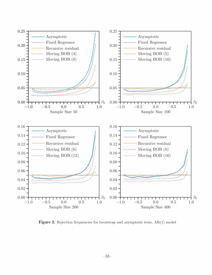
−1.0 −0.5 0.0 0.5 1.00.00

0.05

0.10

0.15

0.20

0.25

...............................................................................................................................................................

........................................................................................................................................................................................................................................................................................................................................................................................................................................................................................................................................................................................

...................................................................................... Asymptotic

...........................................................................................................................................................................

.........................................

..........................................................................................................................................................................................................................................................

............................................................ Fixed Regressor

.......................................................................................................................................................................................

.....................................

.......................................................

.........................

..........

..........

..........

................................................................. Recursive residual

.............................................

.........

........................

............ Moving BOB (4)

...................................................................

.................

............... Moving BOB (8)

Sample Size 50

β2

−1.0 −0.5 0.0 0.5 1.00.00

0.05

0.10

0.15

0.20

0.25

.......................................................................................................................................................................................

..............................................................................................................................................................................................................................................................................................................................................................................................................................................................................................

...................................................................................... Asymptotic

..........................................................................................................................................................................................

..........................................

............................

................................................................................................................................................................................

............................................................ Fixed Regressor

................................................

......................................................................................................

..................................................

........................................

......................................................................

..........

..........

................................................................. Recursive residual

...................................................

...........................

............ Moving BOB (5)

........................................................................

............

............... Moving BOB (10)

Sample Size 100

β2

−1.0 −0.5 0.0 0.5 1.00.00

0.02

0.04

0.06

0.08

0.10

0.12

0.14

0.16

........................................................................................................................................................................

..............................................................

.................................................................................................................................................................................................................................................................................................................................................................................................................................................................................................................................................. Asymptotic

.....................................................................................................................................................................................

...............................................

.................................................................................................................................................................................................................................................................................... Fixed Regressor

....................................................................................................

..........................

.........................................................................................................................................

.................................................................

................................................................. Recursive residual

.....................................................

............................................ Moving BOB (6)

.......................................................................

..................

............... Moving BOB (12)

Sample Size 200

β2

−1.0 −0.5 0.0 0.5 1.00.00

0.02

0.04

0.06

0.08

0.10

0.12

0.14

0.16

..........................................................................................................................................................................................

.....................................................................

...................................................

.....................................................................................................................................................................................................................................................................

...................................................................................... Asymptotic

..................................................................................................................................................................................................................

..............................................

..........................................................................................................................

............................................................ Fixed Regressor

............................................................

..............................

.........................................................................................................

.................................................................

...........................

.......................................

................................................................. Recursive residual

.........................................................

.................

............ Moving BOB (8)

...........................................................................

.........

............... Moving BOB (16)

Sample Size 400

β2

Figure 2. Rejection frequencies for bootstrap and asymptotic tests, AR(1) model

–33–

−1.0 −0.5 0.0 0.5 1.00.03

0.04

0.05

0.06

0.07

0.08

..........

..........

..........

..........

..........

..........

....................................

..............................................................................................

........................................

..............................................

...

.

..........

..............................

..........

..........

...

.......

..........

...

...

...

.

...

..

...

..

..

...

...

..

..

...

...

..

..

...

...

..

..

...

...

..

...

...

..

..

..

...

...

..

..

..

..

..

..

..

..

..

..

..

..

..

..

..

..

..

..

..

..

..

..

..

..

..

..

..

..

..

..

..

..

..

..

..

..

..

..

...

..

.

..

...

..

..

.

................................................................. Recursive residual

..............................................

.........................................................................

............... BC Recursive residual

..................................................................................................................................................................

................................................................................................

......................................................................................................................................................

............................................................ FDB Recursive residual

Sample Size 25

β2

−1.0 −0.5 0.0 0.5 1.00.03

0.04

0.05

0.06

0.07

0.08

..........

..........

....................

........................................

....................................

................................................................

..........

...

...

.............................................................

.................................

........................................

..

...

..

...

...

...

..

..

...

..

...

..

..

...

...

..

...

...

...

.

...

..

...

..

..

..

..

...

.

..

...

..

...

..

..

..

..

..

..

..

..

..

..

..

...

..

..

.

..

..

..

..

..

..

..

..

..

..

..

..

..

...

.

..

..

..

..

..

................................................................. Recursive residual

.....................

....................................................................

..................

............... BC Recursive residual

.......................................................................................................................................................................

..................................................................................................................................................

...............................................................

............................................................ FDB Recursive residual

Sample Size 50

β2

−1.0 −0.5 0.0 0.5 1.00.040

0.045

0.050

0.055

0.060

0.065

...

...

...

.

...

...

....

..........

..........

..........

...

.......

..................................................

........................................

..........

...

.................

......................................................................................................................................................

....................

..

...

...

..

..

..

...

...

...

...

..

..

...

...

..............

..

..

..

..

..

..

..

..

..

..

..

..

..

..

..

..

..

..

..

..

...

..

..

..

.

..

..

..

..

..

...

..

..

..

.

..

..

..

..

..

..

..

..

..

..

..

..

..

..

..

..

..

..

..

..

..

..

..

..

..

..

..

..

..

..

..

..

..

..

..

..

..

..

..

..

................................................................. Recursive residual

...............

.........................

..................

...............................................................

............... BC Recursive residual

.........................................................................................................................................

.......................................................................................................................................

........................

................................................................................................

........................................

............................................................ FDB Recursive residual

Sample Size 100

β2

−1.0 −0.5 0.0 0.5 1.00.040

0.045

0.050

0.055

0.060

0.065

...

...

..

..

..

...

..

...

..........

..........

..........

..............................

..................................................

..............................................................................................................

....................

..........

..............................

..........

....................

...

...

..

..

...

...

...

.

...

...

....

..........

....................

..

..

..

..

..

..

..

...

..

.

..

..

..

..

..

..

..

..

...

.

..

..

..

..

..

..

..

..

..

..

..

..

...

..

.

..

..

..

..

..

..

..

..

..

..

..

..

..

..

..

..

..

..

..

..

................................................................. Recursive residual

.......................................

.............................................................................

............... BC Recursive residual

..........................................

...............................................................................................

......................................................................................................................................................

...................................................................................................................

.................................

............................................................ FDB Recursive residual

Sample Size 200

β2

Figure 3. Rejection frequencies for bootstrap tests, AR(1) model

–34–