Embed Size (px)
Citation preview

Important Notice
This copy may be used only for the purposes of research and
private study, and any use of the copy for a purpose other than research or private study may require the authorization of the copyright owner of the work in
question. Responsibility regarding questions of copyright that may arise in the use of this copy is
assumed by the recipient.
THE UNIVERSITY OF CALGARY
Borehole seismic surveying: 3C-3D VSP and land vertical cable analysis
by
Jitendra Gulati
A THESIS
SUBMITTED TO THE FACULTY OF GRADUATE STUDIES
IN PARTIAL FULFILMENT OF THE REQUIREMENTS FOR THE
DEGREE OF MASTER OF SCIENCE
DEPARTMENT OF GEOLOGY AND GEOPHYSICS
CALGARY, ALBERTA
DECEMBER, 1998
© Jitendra Gulati 1998

ii
THE UNIVERSITY OF CALGARY
FACULTY OF GRADUATE STUDIES
The undersigned certify that they have read, and recommend to the Faculty of Graduate
Studies for acceptance, a thesis entitled “Borehole seismic surveying: 3C-3D VSP and
land vertical cable analysis” submitted by Jitendra Gulati in partial fulfilment of the
requirements for the degree of Master of Science
Supervisor, Dr. Robert R. Stewart
Department of Geology and Geophysics
Dr. Donald C. Lawton
Department of Geology and Geophysics
Dr. Laurence R. Lines
Department of Geology and Geophysics
Dr. Michael A. Slawinski
Department of Mechanical and
Manufacturing Engineering
——————————Date
iii
ABSTRACT
This thesis presents analysis of data from two new borehole seismic methods,
namely the 3C-3D vertical seismic profile (VSP) and the land vertical cable techniques.
Synthetic seismograms and field data from surveys over the Blackfoot oil field in
Alberta, Canada are used for the analysis.
Processing flows for the two techniques are developed. A method that uses
statistical velocity analysis for VSPCDP stacking is also implemented.
Hodogram analysis, median filtering, VSPCDP stack, and f-xy deconvolution are
key steps used in processing the 3C-3D VSP data. Processing of the land vertical cable
data primarily involved predictive deconvolution, velocity filtering, VSPCDP stacking,
and migration.
The structural images from the two techniques are correlated and interpreted with
previously interpreted surface seismic images. Evidence of the productive region (a
Glauconitic sand channel) on the 3-D VSP time slices and on the land vertical cable
image indicate the promise of these techniques.

iv
ACKNOWLEDGEMENTS
My introduction to borehole seismic methods is largely due to the enthusiasm and
inspiration of my supervisor, Dr. Rob Stewart. Through his ideas and feedback, Rob has
been instrumental in teaching me about other fields in geophysics as well. Without his
support and without the opportunities and facilities in CREWES, this thesis would not
have seen the light of day.
Discussions with Dr. Gary Margrave were thoroughly enjoyable and lent a different
perspective about geophysics. Brian Hoffe patiently answered some of my most naïve
questions and was extremely helpful during processing of the land vertical cable data.
Carlos Rodriguez and XinXiang Li have always been there to give geophysical advice
during troubleshooting of data processing. Dan Cieslewicz generously shared his
experiences with the Blackfoot buried geophone experiment.
I would also like to thank Drs. Kurt M. Strack, Arthur Cheng and Janusz Peron at Baker
Atlas, Houston for employing me as a summer intern in 1997. Baker Atlas kindly allowed
me to use their SEISLINK processing package on the Blackfoot 3-D VSP and land
vertical cable data. The 3-D VSP data used in this thesis was partly processed by John
Parkin at Baker Atlas, Calgary. John has been very helpful in giving hints on VSP
processing.
I am fortunate to have loving parents such as mine. They have constantly guided and
understood me. Last but not least, I thank my wife Anupama for without her I would be
doing something other than geophysics.

v
Dedicated to my parents for their love, support, and teachings.

vi
TABLE OF CONTENTS
APPROVAL PAGE ........................................................................................................ii
ABSTRACT...................................................................................................................iii
ACKNOWLEDGEMENTS............................................................................................ iv
DEDICATION................................................................................................................v
TABLE OF CONTENTS ...............................................................................................vi
LIST OF FIGURES......................................................................................................viii
CHAPTER 1: INTRODUCTION ....................................................................................1
1.1 New technologies in vertical seismic profiling ...............................................1
1.2 Introduction to the thesis ................................................................................3
1.3 Hardware and software used ..........................................................................4
CHAPTER 2: VSP MOVEOUT CORRECTION, MAPPING AND POST-VSPCDP-
STACK MIGRATION ....................................................................................................5
2.1 Introduction ...................................................................................................5
2.2 Normal moveout correction of VSP data ........................................................7
2.2.1 Power series expansion for traveltimes of reflected signals in the
VSP geometry ..........................................................................................7
2.2.2 VSP moveout correction method ...................................................11
2.3 Dix interval velocities from VSP data ..........................................................19
2.4 VSPCDP mapping........................................................................................19
2.4.1 VSPCDP mapping equations .........................................................19
2.4.1 VSPCDP mapping of P-wave reflections .......................................21
2.4.2 VSPCCP mapping of converted-wave reflections ..........................24
2.5 Post-VSPCDP stack migration .....................................................................25
2.5.1 Diffractions on VSPCDP stacked data ...........................................29
2.5.2 Synthetic example on post-VSPCDP stack migration.....................31
2.6 Conclusions .................................................................................................35
CHAPTER 3: 3C-3D VSP IMAGING: THE BLACKFOOT EXPERIMENT................36
3.1 Introduction .................................................................................................36
vii
3.2 Acquisition of the Blackfoot 3C-3D VSP.....................................................39
3.3 Processing the 3C-3D VSP data ...................................................................42
3.3.1 Upgoing compressional and shear wavefield separation.................42
3.3.2 P-wave and converted-wave 3-D imaging ......................................45
3.4 P-wave and converted-wave correlation and interpretation ...........................57
3.4.1 P-wave interpretation.....................................................................57
3.4.2 Converted-wave interpretation.......................................................61
3.5 Conclusions .................................................................................................62
CHAPTER 4: LAND VERTICAL CABLE ACQUISITION AND IMAGING..............70
4.1 Introduction .................................................................................................70
4.2 Field description and data acquisition...........................................................72
4.3 Vertical hydrophone cable data versus geophone data ..................................75
4.5 Processing the hydrophone cable data ..........................................................80
4.6 Correlation and interpretation of the hydrophone data ..................................89
4.7 Discussion....................................................................................................91
4.8 Conclusions .................................................................................................92
CHAPTER 5: CONCLUSIONS AND FUTURE WORK ..............................................93
5.1 Thesis conclusions .......................................................................................93
5.2 Future work .................................................................................................94
REFERENCES..............................................................................................................96

viii
LIST OF FIGURES
Fig.2.1. Sorting of surface seismic and VSP data...........................................................12
Fig.2.2. Method to calculate the normal incidence time of VSP reflections ....................14
Fig.2.3. Elastic model used to generate P-P and P-S traveltimes ....................................15
Fig.2.4. Traveltimes for direct and reflected P-wave arrivals for borehole receiver. .......15
Fig.2.5. Normal incidence times estimated after semblance analysis. .............................16
Fig.2.6. Method to calculate the normal incidence time of VSP reflections ....................17
Fig.2.7. Normal incidence P-S times estimated after semblance analysis. ......................18
Fig.2.8. Dix estimates of the model compared with the actual model. ............................18
Fig.2.9. Comparision of mapped reflection points for P-wave reflections ......................22
Fig.2.10. Comparision of mapped reflection points........................................................23
Fig.2.11. Comparison of mapped conversion points.......................................................26
Fig.2.12. Comparision of mapped conversion points......................................................27
Fig.2.13. Comparison of reflection map errors using the converted-wave mapping. .......28
Fig.2.14. Reflection and diffraction arrivals in a VSP geometry.....................................29
Fig.2.15. Model used for generating synthetic data by Kirchhoff diffraction modelling. 32
Fig.2.16. Diffractions from the fault edges.....................................................................33
Fig.2.17. VSPCDP stack of synthetic data. ....................................................................33
Fig.2.18. VSPCDP stacked data in Figure 2.16 after post-stack Kirchhoff migration. ....34
Fig.2.19. Raytracing showing specular reflections from the layer at 1200m depth..........34
Fig.3.1. Map of the Blackfoot surveys ...........................................................................41
Fig.3.2. Processing flow to obtain deconvolved upgoing P-wave and converted-waves..46
Fig.3.3. Shot gathers for shot at an offset of 372m from the well. ..................................48
Fig.3.4. Deconvolved upgoing waves for the same shot gather as in Fig. 3.3. ................49
Fig.3.5. Raw vertical component receiver gather for receiver at depth 655m..................49
Fig.3.6. Raw H1 component receiver gather for receiver at depth 655m.........................50
Fig.3.7. Raw H2 component receiver gather for receiver at depth 655m.........................50
Fig.3.8. Deconvolved upgoing P-waves on vertical component receiver gather..............51
Fig.3.9. Deconvolved upgoing converted-waves on radial component receiver gather ...51
Fig.3.10. Flow for imaging the deconvolved upgoing P-wave and converted-wave........53

ix
Fig.3.11. Fold distribution at the target depth of 1500m.................................................54
Fig.3.12. An inline section from the P-wave 3-D volume obtained from raytracing........54
Fig.3.13. An inline section from the P-wave 3-D volume obtained from semblance. ......55
Fig.3.14. Correlation of the 3-D VSPCDP stacking of P-wave reflections......................55
Fig.3.15. Same inline section as in Figure 3.12 but after f-xy deconvolution. .................56
Fig.3.16. An inline section from the converted-wave 3-D volume..................................58
Fig.3.17. Same inline section as in Figure 3.16 but after f-xy deconvolution. .................58
Fig.3.18. 3-D VSP P-wave correlation with migrated surface 3-D P-wave data..............59
Fig.3.19. P-wave time slice at the channel level from the raytraced VSPCDP volume....59
Fig.3.20. P-wave time slice at the channel level from the semblance VSPCDP volume..60
Fig.3.21. P-wave time slice at the channel level from the migrated surface 3-D volume.60
Fig.3.22. P-wave time slice at the channel level for the entire surface 3-D survey .........63
Fig.3.23. VSP P-wave time slice at the channel level from Figure 3.17 inset . ...............64
Fig.3.24. 3-D VSP converted-wave correlation with 3-D converted-wave data ..............65
Fig.3.25. Correlations between synthetic and different data ...........................................59
Fig.3.26. Converted-wave time slice at the channel level from the 3-D VSP. .................67
Fig.3.27. Converted-wave time slice at the channel level from the surface 3-D..............67
Fig.3.28. Converted-wave time slice at the channel level from the surface 3-D..............68
Fig.3.29. VSP Converted-wave time slice at the channel level inset...............................69
Fig.4.1. Map showing the location of the PanCanadian Blackfoot field..........................73
Fig.4.2. A schematic diagram of the Blackfoot 3C-2D survey (not to scale)...................74
Fig.4.3. Receiver gather for hydrophone at 18m depth...................................................77
Fig.4.4. Receiver gather for vertical component geophone at 18m depth........................78
Fig.4.5. Receiver gather for inline horizontal component geophone at 18m depth. .........78
Fig.4.8. Amplitude spectrum of stacked receiver gather.................................................79
Fig.4.7. Hydrophone vertical cable processing flow.......................................................82
Fig.4.9. Raw receiver gather for hydrophone at 98m depth after shot statics. .................83
Fig.4.10. Same receiver gather as in Fig.4.9 but after predictive deconvolution. ............84
Fig.4.11. Same receiver gather as in Fig.4.10 but after f-k filtering of shot gathers.........85
Fig.4.12. Shot gathers after application of gain. .............................................................86
Fig.4.13. Shot gathers in Fig.4.12 after predictive deconvolution...................................86

x
Fig.4.14. Shot gathers in Fig.4.13 after f-k filtering........................................................87
Fig.4.15. VSPCDP stacked section of the hydrophone data............................................88
Fig.4.16. f-x deconvolution of the whitened VSPCDP stack in Figure 4.15....................88
Fig.4.17. Post-stack migration of whitened VSPCDP stack in Figure 4.15. ....................89
Fig.4.18. Migrated hydrophone traces near the borehole spliced into a seismic section. .90
Fig.4.19. Migrated hydrophone traces inserted into a 3-D crossline. ..............................90
Fig.4.20. Interpreted hydrophone data. ..........................................................................91

1
CHAPTER 1: INTRODUCTION
1.1 New technologies in vertical seismic profiling
The vertical seismic profiling (VSP) is a technique in which seismic signals generated at
the surface of the earth are recorded by geophones at various depths in a borehole. The
VSP has found a number of applications in the oil industry. Primarily, VSP data have
been used to assist surface seismic interpretation through time-to-depth values and a zero-
phase, largely multiple-free reflectivity trace. It has given insight into the nature of
seismic wave propagation in the earth and provided estimates of rock properties such as
interval velocities and attenuation near the borehole. Detailed descriptions about the
history and applications of the VSP can be found in Hardage (1983) and in Toksoz and
Stewart (1984). Hardage (1992) also describes the reverse VSP (RVSP) technique in
which seismic signals generated by a source in a borehole are recorded by receivers at the
surface of the earth.
Most VSP surveys to date have either been 1-D (source near the well head) or 2-D
(sources in a line out from the well). But the inherent 3-D nature of the earth and a desire
to obtain detailed 3-D reservoir information near the well has led to interest in acquiring
some type of 3-D data in boreholes. Basically, a 3-D VSP survey is a measurement of
seismic signal in borehole detectors using an areal distribution of surface shots. One of
the first 3-D VSP surveys is that conducted by AGIP in 1989 in the Brenda field, but it
has only been recently that 3-D VSP surveys have started appearing in the public domain.
A 3-D VSP conference held in Stavanger, Norway in 1997 and a session dedicated to 3-D

2
VSP in the Annual SEG Meeting at New Orleans in 1998 are some indicators of the
growing interest in 3-D borehole seismic data.
Another area that has recently received renewed interest is the use of hydrophones in
acquiring VSP data. Hydrophones offer a rapid and efficient way to acquire VSP data
and hence the interest in them. White and Sengbush (1953) and Riggs (1955) were
among the first to use hydrophone detectors in acquiring borehole seismic data. Tube
waves are the primary stumbling block in the use of hydrophone data. Therefore,
properly clamped geophones, which are less sensitive to tube waves, have been the
preferred detectors so far. Recently, Findlay et al. (1991), Milligan et al. (1997) and
Sheline (1998) demonstrated the viability of using a vertical hydrophone array in their
borehole reflection imaging programs.
The marine vertical cable is another new technology that is closely related to the VSP
method (Krail, 1994a; Krail, 1994b). In this technique, a cable consisting of a set of
vertically separated hydrophone detectors is suspended in water with the help of an
anchor at the sea bottom and bouyant floats under the water surface. Krail (1994b)
mentions that the marine vertical cable resulted in significant reduction in cost and
acquisition speed in a survey over the Gulf of Mexico. He also indicates that the vertical
cable resulted in a better image compared to the image from a conventional towed
streamer data.

3
3-D VSP surveys and the use of vertical hydrophone arrays on land (henceforth referred
to as land vertical cable) in shallow or deep boreholes are the subject of this thesis.
Techniques relevant to the efficient processing of these data are developed and
investigated; and real data examples from such surveys analyzed, processed and
interpreted in this work. The following sections give an outline of this thesis.
1.2 Introduction to the thesis
Chapter 2 of the thesis is a theoretical development of a VSPCDP mapping technique.
Synthetic data are used for comparing the technique with raytrace VSPCDP mapping;
thus highlighting its advantages and limitations. Finally, the feasibility of using a
standard post-stack migration routine to VSPCDP stacked data is investigated.
Chapter 3 discusses the acquisition, processing and interpretation of real 3-D VSP data.
The data used in this chapter is from the 3-D VSP survey shot over the Blackfoot field,
which is owned by PanCanadian Petroleum Ltd., in Canada in 1995. This survey (to our
knowledge) is the first simultaneous acquisition of a 3-D VSP along with a surface 3-D
survey. Detailed descriptions about the survey are given in the chapter. The processing
flow used to obtain the final interpretable P-wave and converted-wave time slices from
the 3-D VSP data is discussed. Final images from the 3-D VSP data are then correlated
with images from the surface 3-D, an offset VSP and synthetic seismograms and
interpreted.
Chapter 4 is about land vertical cable acquisition and imaging. The data used in this
chapter was obtained during November, 1997 as part of a series of 2-D seismic
4
experiments over the Blackfoot field (see Hoffe et al., 1998 for details). The vertical
cable data were recorded by deploying a 48-channel hydrophone cable in a 100m deep,
cased and water-filled hole. Acquisition parameters of the data are discussed in this
chapter. This is followed by developing a processing flow for land vertical cable data.
The processed data are then correlated with 2-D and 3-D images from the same area and
finally interpreted.
Chapter 5 provides the final conclusions of the thesis. Future work to improve the 3-D
VSP processing flow are also suggested.
1.3 Hardware and software used
The entire work presented in this thesis was performed on the Sun workstation and PC
network of the CREWES Project at the University of Calgary. The testing of the
VSPCDP mapping techniques was done in the Matlab environment. An existing Matlab
P-S raytracing code was adapted to the VSP geometry for this purpose. The
implementation of the VSPCDP mapping technique on real data was performed by
writing C source codes in Western Atlas Logging Services (WALS) SEISLINK
processing package. The 3-D VSP data, as well as the land vertical cable data, were
processed using both SEISLINK and ProMax processing packages. Word and image
processing for the thesis assembly were performed in MICROSOFT WORD and ADOBE
PHOTOSHOP software respectively.
5
CHAPTER 2: VSP MOVEOUT CORRECTION, MAPPING AND POST-VSPCDP-STACK MIGRATION
2.1 Introduction
Offset and walkaway VSP surveys have been useful in extracting structural information
near the well. The structural image from the VSP is, in many cases, obtained from the
VSPCDP stacking process (Wyatt and Wyatt, 1984). VSPCDP stacking is an analogue of
the surface seismic CMP stacking process. VSPCDP stacking is, however, a more
complicated process than CMP stacking. It first involves normal-moveout (NMO)
correction. NMO correction is followed by mapping the reflections to their spatial
locations and subsequently stacking the data to give an offset-time image.
Raytracing can be used to correct VSP data to normal incidence time (Wyatt and Wyatt,
1984). Velocity information from well-logs, known geology of the area or from surface
seismic in the area, and often traveltime inversion of the VSP first-breaks (Stewart, 1984)
provide a starting velocity-depth model for raytracing. As both the geometry and
frequency content of VSP data are different compared to well-log or surface seismic data,
these starting estimates are not optimum for the NMO correction of the VSP data. Also,
in the simple case of a horizontally layered earth, velocity anisotropy further complicates
determination of the optimum model for the VSP data (Dillon and Thomson, 1984). Thus
moveout correction can be a time-consuming process especially for walkaway or 3-D
VSPs where the data volume is large and model building comparatively difficult.
6
Other moveout correction methods such as in Moeckel (1986) and Zhang et. al. (1995)
also require a velocity model. These methods calculate the RMS velocity from a model to
correct the VSP data to normal incidence time. However, from surface seismic surveys,
we know that the stacking velocity is greater than the RMS velocity (Al-Chalabi, 1973).
One would then expect that, in a similar way, the above approximation methods may not
give the optimum stack for VSP data as well. In such a case, a statistical moveout
correction method similar to amplitude semblance analysis (Taner and Koehler, 1969)
used in surface seismic surveys may be more desirable. Byun et. al. (1989) used
amplitude semblance analysis in their study of anisotropic velocities from VSP data.
However, I am not aware of a method described in literature to correct VSP data to
normal incidence time using semblance analysis.
After the final velocity-depth model is built, reflections on moveout-corrected VSP data
are mapped to their subsurface spatial locations by raytracing through the model (Wyatt
and Wyatt, 1984). This process is referred to as VSPCDP transformation or mapping.
Although a raytracing approach is accurate in mapping the reflection points, approximate
mapping methods such as Stewart (1991) also perform with reasonable accuracy in
simple geology. In the case of a 3-D VSP, 3-D raytracing may be a time-consuming
process and likely to be unnecessary in a simple geology.
In this chapter, a method is developed for the rapid VSPCDP stacking of VSP data and
tested on synthetic VSP data. The possibilities and limitations of applying a standard
post-stack migration routine to VSPCDP stacked data are also investigated.

7
2.2 Normal moveout correction of VSP data
Taner and Koehler (1969) used a power series expansion of the parametric traveltime-
distance equations and showed that the offset-traveltime relation is a hyperbola for
surface seismic surveys. This relation provides a framework for normal moveout (NMO)
correction of surface recorded signals in the common midpoint (CMP) domain. In the
following, an equivalent series expansion for VSP-recorded signals is presented which
shows that the traveltime-distance formula is hyperbolic for VSP- recorded signals as
well. This relation provides an opportunity to NMO-correct VSP records, similar to that
performed in surface seismic surveys.
2.2.1 Power series expansion for traveltimes of reflected signals in the VSP geometry
Taner and Koehler (1969) expanded the traveltime of reflected waves recorded on the
surface over a horizontally layered medium into a power series as
t x c c x c x c xn2 2
1 22
34
46( ) ......= + + + + , (2.1)
where the coefficients ic (i=1,2,3,..) are functions of the thickness and velocity of the
layers, and nt is the traveltime for reflection at the n-th layer with source at an offset x
from the receiver.
Using arguments as in Taner and Koehler (1969), one can obtain a similar result for the
VSP geometry as well. The asymmetry of the downgoing and upgoing raypaths in the
VSP geometry makes the derivation similar to that for converted waves as in Tessmer
and Behle (1988). However, I was unaware of this similarity when deriving the following
relations for P-wave arrivals in the VSP based on the Taner and Koehler (1969)
derivation.

8
In a horizontally layered medium, the t-x relationship for reflections recorded in a
borehole can be expressed in the parametric form (Slotnick, 1959) as
xpv d
p v
pv d
p v
k k
kk
k nj j
jj n
j m
=−
+−=
=
=
=
∑ ∑1 12 2
12 2
, and
td v
p v
d v
p v
k k
kk
k nj j
jj n
j m
=−
+−=
=
=
=
∑ ∑1 12 2
12 2
where vk and d k are the P-wave velocity and thickness of the k-th layer and p is the ray
parameter given by Snell’s law as
pv
k
k
=sinθ
, where θk is the angle of incidence of the ray at the k-th layer.
Here for the sake of brevity, I assume that the receiver is located at the base of the (m-1)th
layer. This assumption, however, does not make a difference in the final result.
Using a Taylor series expansion of the function ( )1 2 2 1 2− −p vk , the above equations can be
rewritten as
x pv di
ip v pv d
i
ip vk k
k
k n
i
ik
ij
j n
j m
ji
ji
i
=−−
+−−=
=
=
∞− −
=
=− −
=
∞
∑ ∑ ∑ ∑1 1
2 2 2 2 2 2 2 2
1
135 2 3
2 4 6 2 2
135 2 3
2 4 6 2 2
. . .....( )
. . .....( )
. . ....( )
. . .....( )
=−−
+=
∞− + −
=
=+ −
=
=
∑ ∑ ∑135 2 3
2 4 6 2 21
2 1 2 1 3
1
2 1 3. . ....( )
. . ....( )[ ]( ) ( )i
ip v d v d
i
ik
i
k
k n
k ji
j n
j m
j (2.2)
Let q1 1= , qi
ii =−−
135 2 3
2 4 6 2 2
. . ....( )
. . ....( ) and
j
mj
nj
ij
nk
kk
iki dvdva ∑∑
=
=
−=
=
− += 32
1
32 ;
Substituting the above in (2.2) gives

9
x q a pii
ii=
=
∞
+−∑
11
2 1
Let b q ai i i= +1 , and,
x b pii
i==
∞−∑
1
2 1 (2.3)
Similarly, letting γ i i iq a= , we get
22
1
−∞
=∑= i
ii pt γ (2.4)
Substituting (2.3) and (2.4) in (2.1) and comparing like powers of p2 gives us the
coefficients of the power series in (2.1). Following Taner and Koehler (1969), the
coefficients are calculated as follows:
c q a ad
v
d
vtk
kk
k nj
jj n
j m
r1 12
1 12
12
1
202= = = = + =
=
=
=
=
∑ ∑γ [ ] (2.5)
where t r0 is the zero-offset traveltime for the reflected P-wave arrival to the receiver in
the borehole.
Similarly, ca
a
d v d v
d v d vv
k kk
k n
j jj n
j m
k k j jj n
j m
k
k n21
2
1
1
2
1= =
+
+=
=
=
=
=
=
=
=
=
∑ ∑
∑∑ ( ) (2.6)
where v can be defined as the rms velocity for the reflected P-wave arrival with respect
to the nth reflector at the particular receiver depth.
We can derive other coefficients as well, however, a two-term truncation suffices, as
evidenced later in this thesis. Therefore, the traveltime-distance relationship for the
reflected P-wave arrivals at a receiver in a borehole can be written in the hyperbolic form

10
t tx
vr2
02
2
2= +( )
. (2.7)
Similarly, for direct arrivals at the receiver we find
20
21
11 ][ d
mj
j j
j tv
dc == ∑
−=
=
(2.8)
where t d0 is the zero-offset traveltime for the direct arrival to the receiver in the
borehole.
Furthermore, 21
1
1
12
)(
1
vvd
vd
cmj
jjj
mj
jjj
==
∑
∑−=
=
−=
= (2.9)
where v is the rms velocity for the direct arrival at the receiver.
Thus, a two-term truncation of the power series expansion for direct arrivals gives the
hyperbolic t-x relationship
t tx
vd2
02
2
2= +( )
(2.10)
Tessmer and Behle (1988) showed that a hyperbolic approximation to traveltimes can be
used for converted-wave arrivals on the surface. Since in the VSP, asymmetry in the
raypath is common to both pure P-wave and converted-wave arrivals, we simply extend
the formula for pure P-wave arrivals (Equation 2.7) to the converted-wave arrivals in the
VSP to give the relation
2
220
2
)( PS
PSv
xtt += (2.11)
11
where PSt0 is the zero-offset traveltime to the borehole receiver for the converted-wave
reflection. PSν is the corresponding rms velocity given by
2
1
1
2
12 )(
1
PSnk
k
mj
njjjkk
mj
njjj
nk
kkk
dvd
dvd
a
ac
νβ
β=
+
+==
∑ ∑
∑∑=
=
=
=
=
=
=
= (2.12)
jβ is the shear-wave velocity of the j-th layer.
The convergence properties of the traveltime expansions are the same as discussed in Al-
Chalabi (1973).
2.2.2 VSP moveout correction method
Unlike surface recorded signals, the locus of reflection points for each source-receiver
pair in VSP surveys depends on reflector depth. It tends towards the source-receiver
midpoint with increasing depth in a horizontally layered earth (see Dillon and Thomson,
1984 for excellent examples). Therefore, VSP data cannot be sorted simply in the CMP
domain as in surface seismic surveys. Also, the RMS velocity (Equation 2.6) for reflected
signals in the VSP geometry changes with the receiver depths/locations. This implies that
to use the inherent data redundancy, VSP data needs to be sorted in the receiver domain
for implementation of a NMO correction method similar to the one used in surface
seismic surveys. Figure 2.1 shows the difference between the sorting of surface seismic
and VSP data.

12
S4 S3 S2 S1 R1 R2 R3 R4
(a)
S1 S2 S3 S4
R
(b)
Fig.2.1. (a) Surface seismic data sorted in the CMP domain. (b) VSP data sorted in the
receiver domain.

13
2.2.2.1 Moveout correction of pure P-wave arrivals
After the vertical component data are sorted into the receiver domain, Equation (2.10) is
used on the first-break picks to get the zero-offset time of the direct arrivals (t0d). Further,
amplitude semblance analysis (see Taner and Koehler, 1969 for details) of the reflected
arrivals based on Equation (2.7) gives the zero-offset time (t0r) for each of the reflected
arrivals in the sorted data. The quantities t0d and t0r are then added to obtain the normal
incidence time of the reflected arrivals. Figure 2.2 shows the steps followed in correcting
the reflected arrivals to normal incidence time.
2.2.2.2 Moveout correction of converted-wave arrivals
To correct converted waves to normal incidence P-S times in a manner similar to the
procedure outlined in Figure 2.2, one would need the downgoing direct S-wave arrival
times. These may be available in the form of S-wave arrivals from P-S transmissions near
the surface. When these are not available, one can approximately calculate the zero-offset
time for a downgoing S-wave from the P-wave direct arrivals assuming a constant P-
wave/S-wave velocity ratio. Equation 2.11 is then used to calculate the zero-offset time
of a converted-wave reflection from amplitude semblance analysis. In Figure 2.6, a
schematic diagram is shown to correct the converted-wave arrivals to approximate
normal incidence P-S times using P-wave direct arrivals.
14
2.2.2.3 Synthetic results of the moveout correction methods
Raytracing was used to generate synthetic P-wave traveltimes for a model (Figure 2.3).
Traveltimes were calculated for borehole receivers placed at depths 400m and 910m with
source offsets varying from 50m to 1950m. These times were calculated for the model
with maximum depth of reflection being 2000m. Figure 2.4 shows the traveltimes of the
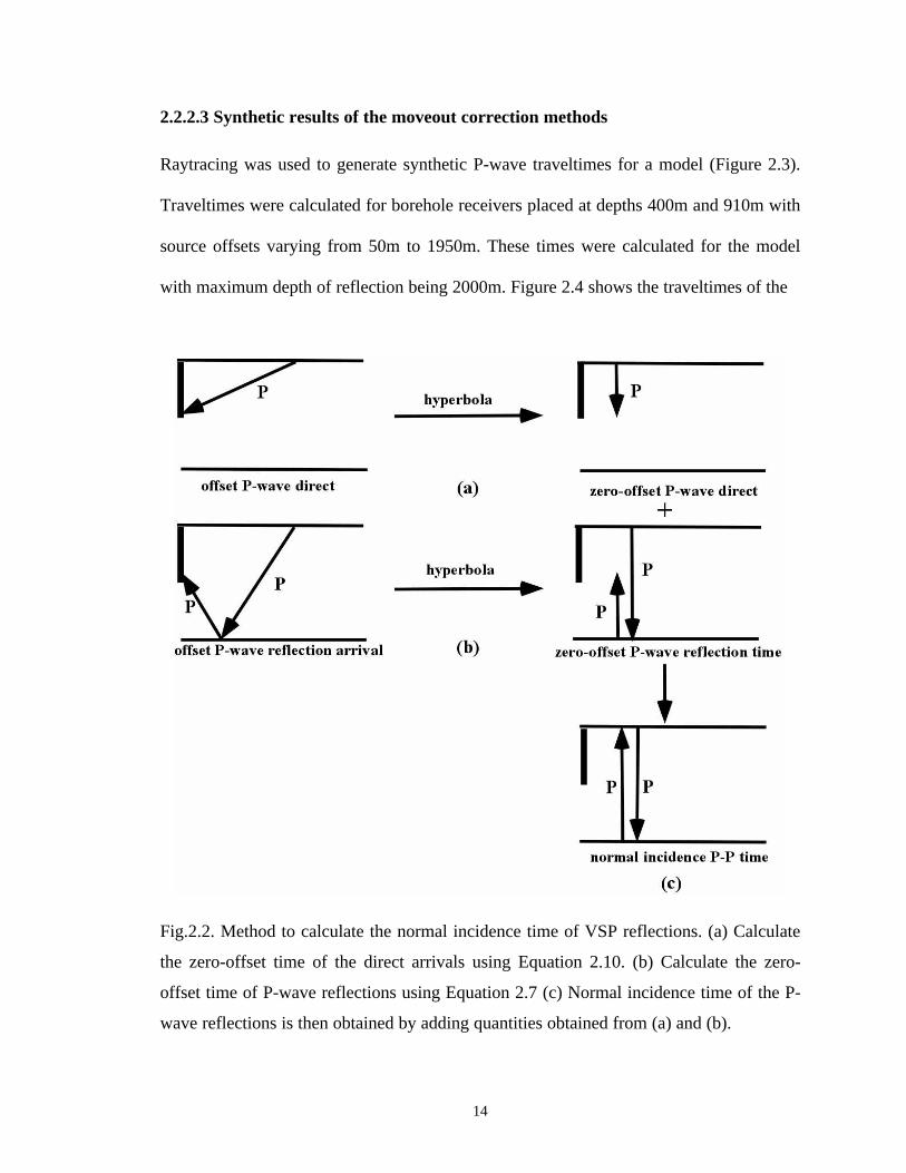
Fig.2.2. Method to calculate the normal incidence time of VSP reflections. (a) Calculate
the zero-offset time of the direct arrivals using Equation 2.10. (b) Calculate the zero-
offset time of P-wave reflections using Equation 2.7 (c) Normal incidence time of the P-
wave reflections is then obtained by adding quantities obtained from (a) and (b).

15
Fig.2.3. Elastic model used to generate P-P and P-S traveltimes for borehole geometries
(from Zhang et al., 1996)
Fig.2.4. Traveltimes for direct and reflected P-wave arrivals for borehole receiver at a
400m depth of the model in Figure 2.3.

16
(a) Normal incidence times for receiver
depth at 400m.
(b) Normal incidence times for receiver
depth at 910m.
Fig.2.5. Normal incidence times estimated after semblance analysis match remarkably
well with the actual times. Circles indicate the times estimated from the method in Figure
2.2 where the line passing through these are the actual times.
P-wave reflected arrivals for the model with borehole receiver at 400m depth; the first
event representing the P-wave direct arrival. Following the steps outlined above, normal
incidence times (Figure 2.5) for reflection events were determined for both receiver
depths. To simulate amplitude semblance analysis, a least-squares solution to the
traveltimes was used to calculate the normal incidence time. The estimated times match
remarkably well with the true zero-offset times, with maximum error being less than 2ms.
Next, synthetic converted-wave traveltimes were used to test the method for converted-
waves. The synthetic converted-wave traveltimes were generated for the same model
(Figure 2.3) using raytracing for the same source-receiver geometry. Following the steps
outlined in Figure 2.6, normal incidence P-S times were determined for converted-waves
assuming a SP V/V ratio of 1.75 (Figure 2.7). Times estimated using the method in

17
Figure 2.6 match well with actual calculated times, the maximum error being less than
7ms.
Fig.2.6. Method to calculate the normal incidence time of VSP reflections. (a) Calculate
the zero-offset time of the direct arrivals using Equation 2.10. Multiply it by an assumed
VP/VS to get approximate zero-offset time of a downgoing S-wave. (b) Calculate the
zero-offset time of converted-wave reflections using Equation 2.11. (c) Normal incidence
time of the converted-wave reflections is then obtained by adding quantities obtained
from (a) and (b).

18
(a)Normal incidence P-S times for
receiver depth at 400m.
(b)Normal incidence P-S times for
receiver depth at 910m.
Fig.2.7. Normal incidence P-S times estimated after semblance analysis match
remarkably well with the actual times. Circles indicate the times estimated from the
method in Figure 2.6 where the line passing through these are the actual times.
Fig.2.8. Dix estimates of the model compared with the actual model.
19
2.3 Dix interval velocities from VSP data
Equation 2.9 results in the same formula nn
nnnn
n tt
tvtvv
−−
=+
++
1
2
1
21
for the P-wave interval
velocity as in Dix (1955). Estimates of interval velocities obtained during moveout
correction of the synthetic P-P traveltimes are compared with the actual model (Figure
2.8). The estimated velocity-depth model using the Dix formula is very close to the actual
model despite the assumption of stacking velocities being equal to the RMS velocities.
When events are closely spaced in time, the estimates deviate more from the actual
values as observed in the case of the last two events.
2.4 VSPCDP mapping
The advantage of doing the NMO correction of VSP data using the method described in
previous sections is that it does not require a model. However, standard procedure for
VSPCDP mapping involves raytracing through a model to map the spatial locations of
reflections. In such a case, methods that use information obtained from semblance
analysis are required to map the reflection points. Approximate mapping methods such as
in Stewart (1985) and Stewart (1991) are easily adapted to serve the above purpose and
are shown in the following section.
2.4.1 VSPCDP mapping equations
The offset xB of the reflection point from the well for a P-wave arrival over a
homogeneous single-layered earth is given in Stewart (1985) as

20
xx vt z
vt zBv
v
=−−2
2[ ] (2.13)
where x v t zv, , , are the source-receiver offset, constant velocity of the homogeneous
single-layered medium, normal incidence time of reflection and depth of the receiver
respectively. Equation 2.13 which is valid for a single-layered is adapted to a multi-
layered earth by simply substituting the stacking velocity v (assumed equal to RMS
velocity) in place of the constant velocity v .
Another formula that can be used for mapping both P-wave and converted-wave
reflections is given in Stewart (1991) as
oU
2U
oD
2D
B
tV
tV1
xx
+
= (2.14)
where UD V V , are the RMS velocities, and oUoD t ,t are the zero-offset time for the
downgoing and upgoing waves respectively.
The quantities in the denominator in Equation 2.14 can be determined as
γ+−
+=11
tVtVtVtV od
2dor
2r
od
2doD
2D
(2.15)
where ort and odt are the zero-offset times, and rV and dV are the RMS velocities for the
reflected and direct wave respectively. These values are obtained during NMO correction
of VSP data using the method discussed in the previous sections. γ is the P-wave to S-
wave interval velocity ratio and is assumed to be a constant for the entire model. γ =1 in
the case of P-wave reflections.
The other quantity in Equation 2.14 is then determined as
21
oD
2Dor
2roU
2U tVtVtV −= (2.16)
2.4.1 VSPCDP mapping of P-wave reflections
Synthetic traveltimes from previous sections are used for testing the accuracy of the
approximate methods. For comparison, reflection points were mapped using a 2-D
raytracing and both of the approximate mapping procedures. Stacking velocities and
normal incidence times for P-wave reflections obtained from moveout correction of the
P-wave synthetic traveltimes are used in the calculations.
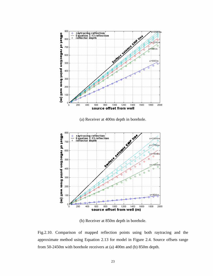
From Figure 2.9, we observe that the approximate reflection points at small source offsets
are accurate when compared to those obtained from raytracing. Even at a large offset of
1950m, the approximate mappings are reasonable relative to bin size. Figure 2.10
displays the reflection point maps for all source-receiver offsets for reflections recorded
at receiver depths of 400m and 850m respectively. It can be seen that the accuracy of the
approximate methods decreases with increasing offset and receiver depth. However, in a
VSP the maximum source offset is usually equal to the depth of the reflector of interest.
Within this limit, the mapping methods are as good as raytracing for the simple earth
model of Figure 2.3. Therefore, in a simple geology the final image will nearly be the
same using either of the mapping methods.

22
(a) Source at 50m offset
(b) Source at 1950m offset
Fig.2.9. Comparison of mapped reflection points for P-wave reflections using raytracing
and approximate mapping methods for borehole receiver at 400m depth.
23
(a) Receiver at 400m depth in borehole.
(b) Receiver at 850m depth in borehole.
Fig.2.10. Comparison of mapped reflection points using both raytracing and the
approximate method using Equation 2.13 for model in Figure 2.4. Source offsets range
from 50-2450m with borehole receivers at (a) 400m and (b) 850m depth.

24
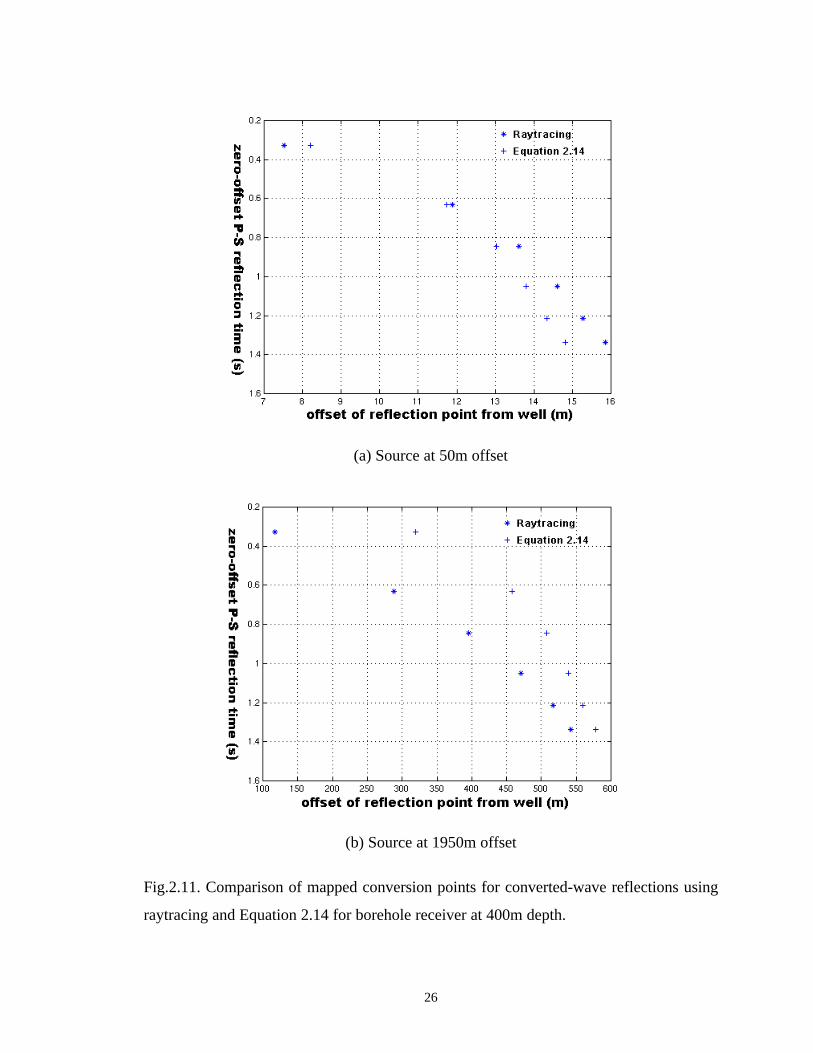
2.4.2 VSPCCP mapping of converted-wave reflections
Equations 2.14-2.16 are used for mapping the converted-wave reflection points. Synthetic
converted-wave traveltimes computed in previous sections were used for testing the
accuracy of the mapping method. Stacking velocities and zero-offset times used in the
equations were obtained from amplitude semblance analysis of the converted-wave
synthetic. Values around 0.2=γ for the model resulted in reflection points closest to that
obtained from raytracing. These are shown and compared with reflection maps obtained
from raytracing (Figure 2.11). The average and time-weighted average γ values for the
synthetic traveltimes was found to be 1.81 and 1.79 respectively. From this, it appears
that γ values slightly higher than the average or a time-weighted average should be used
in the computation of the approximate reflection maps.
From Figure 2.11, we observe that the approximate reflections are again accurate at small
source offsets when compared to those obtained from raytracing. However, at the far
offset of 1950m, the approximate mappings have large errors at shallow depths which
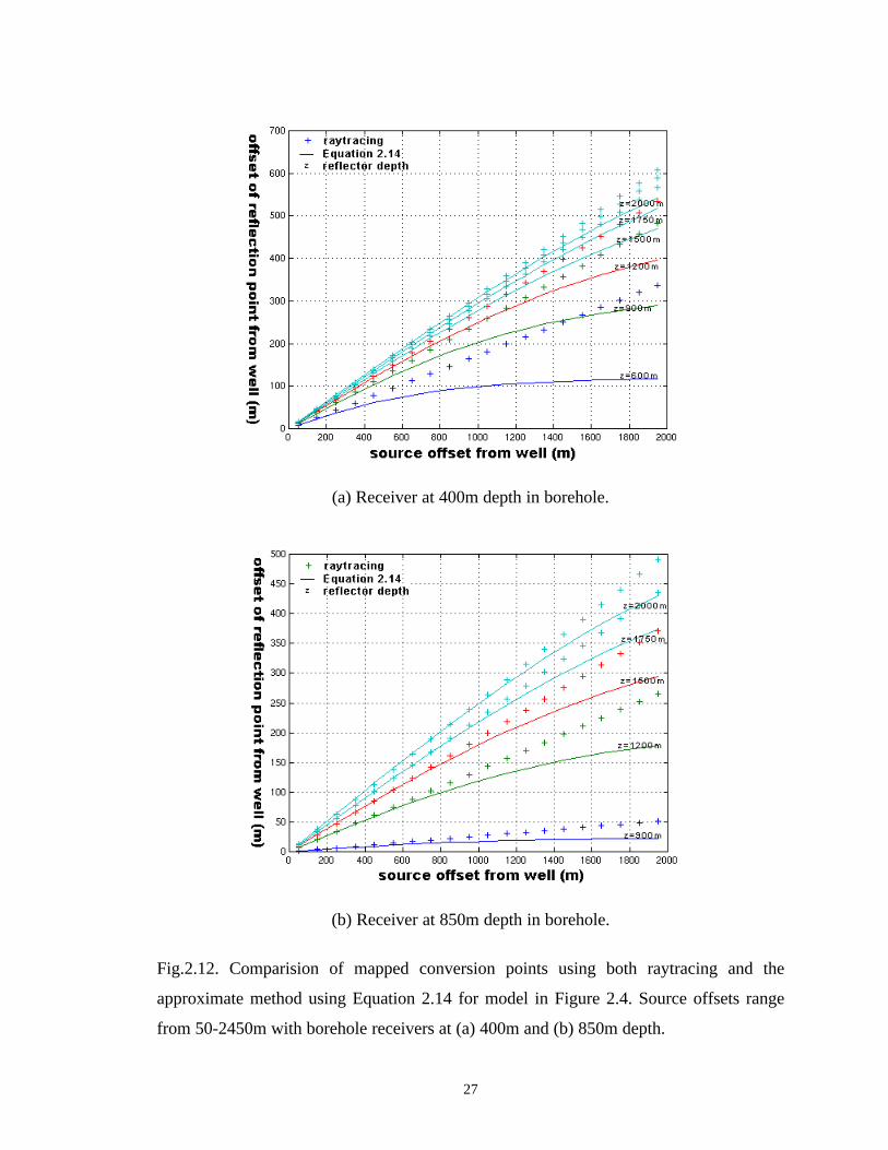
decreases with increasing depth of the reflectors. Figure 2.12 displays the reflection point
maps for all source-receiver offsets for reflections recorded at receiver depths of 400m
and 850m respectively. The increase in accuracy with reflector depth is due to a larger P-
wave leg in the converted-wave reflection and also on effective smaller source offset-to-
depth ratio. We observe that application of the mapping equation to converted-waves is
restricted to the zone where the lateral movement of the reflection point is a linear
function of the source offset.

25
Reflection maps were also calculated for a range of γ values for studying the effect of
errors in the γ value (Figure 2.13). The errors in the figure are relative to the reflection
map for 0.2=γ value, assuming that in a particular area this value gives reflection maps
closest to those obtained from raytracing. It can be seen that even small errors in γ values
result in high errors. It appears that it would be more appropriate to use raytracing than an
approximate equation for VSPCCP mapping.
2.5 Post-VSPCDP stack migration
Methods discussed in the above sections assumed a simple stratified earth model.
Limitations of reflection mapping methods discussed in the previous sections for dipping
layer earth models are well-known. It should also be noted that for the VSP geometry in
the dipping layer case, solving for the hyperbola for zero-offset time is not equivalent to
solving for normal incidence time. In surface seismic surveys, both zero-offset and
normal incidence times are considered equivalent. Moreover, the VSPCDP stacking
methods are not capable of collapsing diffractions.
This would mean unfocussed fault edges, incorrect dips, and therefore,
misinterpretations. In the case of surface seismic data, the conventional approach to
handle diffractions is to use a post-stack migration routine using the exploding reflector
model (Loewenthal et al., 1976). In the VSP, however, the asymmetry of raypaths and
subsequent VSPCDP stack are believed to complicate diffraction patterns on the stacked
section.
26
(a) Source at 50m offset
(b) Source at 1950m offset
Fig.2.11. Comparison of mapped conversion points for converted-wave reflections using
raytracing and Equation 2.14 for borehole receiver at 400m depth.
27
(a) Receiver at 400m depth in borehole.
(b) Receiver at 850m depth in borehole.
Fig.2.12. Comparision of mapped conversion points using both raytracing and the
approximate method using Equation 2.14 for model in Figure 2.4. Source offsets range
from 50-2450m with borehole receivers at (a) 400m and (b) 850m depth.

28
Fig.2.13. Comparison of reflection map errors using the converted-wave mapping
equation with a range of γ values.
Thus, data acquired in a VSP geometry is usually migrated before stack using methods
such as those discussed in Chang and McMechan (1986), Kohler and Koenig (1986), and
Whitmore and Lines (1986). If diffractions on VSPCDP stack do not have a regular
pattern, then it may be advantageous to an interpreter. On the other hand, if they do
follow a certain pattern then it would be worthwhile to investigate if surface seismic
migration routines can be used to enhance interpretation. The problem is analogous to
post-stack converted data recorded on the surface of the earth and is discussed in the
following sections.

29
2.5.1 Diffractions on VSPCDP stacked data
Consider the VSP geometry in Figure 2.14 where a specular reflection occurs at a
distance cx and a diffraction at a further distance R from it. The traveltime rt for the
specular reflection is then given by the double square-root equation as
[ ] [ ]{ }212c
2212c
2r x)zD()xx(D
v
1t +−+−+=
which can be written as
[ ] [ ]{ }212c
22212c
2r x)Dz2z(D)xx(D
v
1t +−++−+= . Assuming that the moveout
contributions are small compared to normal incidence time, the traveltime can
approximately be written as
+−++
−+=
2
2c
2
2
2c
rD2
xDz2z1D
D2
)xx(1D
v
1t ,
i.e.,
+
−+−+=
Dv2
x
Dv2
)xx(
Dv2
Dz2z
v
D2t
2c
2c
2
r . (2.17)
Fig.2.14. Reflection and diffraction arrivals in a VSP geometry.

30
The traveltime for the diffraction in the figure is given by
[ ] [ ]{ }212c
2212c
2d )Rx()zD()Rxx(D
v
1t ++−+−−+= . (2.18)
By repeating the same procedure as in the previous case, the diffraction traveltime can be
approximated to
R)xx2(Dv
1
Dv
R
Dv2
x
Dv2
)xx(
Dv2
Dz2z
v
D2t c
22c
2c
2
d −++
+
−+−+= (2.19)
From Equations 2.17 and 2.19, the residual time rdt for the diffraction after NMO
correction is
R)xx2(Dv
1
Dv
R
v
D2t c
2rd −++= (2.20)
Now let us consider two extreme cases. First consider the case in which the receiver is
closer to the reflector such that Dz → and, therefore, xxc << . Then Dv
xR
Dv
R
v
D2t
2rd −+≈
and thus the diffraction residual is dependent on the geometry as well. Some sort of pre-
stack operator would, therefore, be required so as to apply a standard migration routine
on stacked VSP data.
Now consider the case in which the receiver is closer to the surface than to the reflector
such that Dz0 <<< . In such a case, the reflection point would tend towards the mid-
point of source-receiver offset i.e. 2xxc → . Therefore, Dv
R
v
D2t
2rd +≈ . Squaring and

31
neglecting the term raised to the power of four results in the familiar hyperbola relation
for the surface seismic and given as
2
2
2
2 442
v
R
v
Dt r
d +≈ . Thus, standard surface seismic migration routines could be applied to
a VSPCDP stacked section under the above limitation.
2.5.2 Synthetic example on post-VSPCDP stack migration
We saw the limitations of applying a migration operator to a VSPCDP stacked section in
the previous section. Nonetheless, valuable information could be obtained if the data
could be migrated with reasonable success. This information could then provide
additional knowledge for building the velocity-depth model for pre-stack depth
migration. Synthetic data are tested to evaluate the performance of a post-stack migration
operator on VSPCDP stacked data.
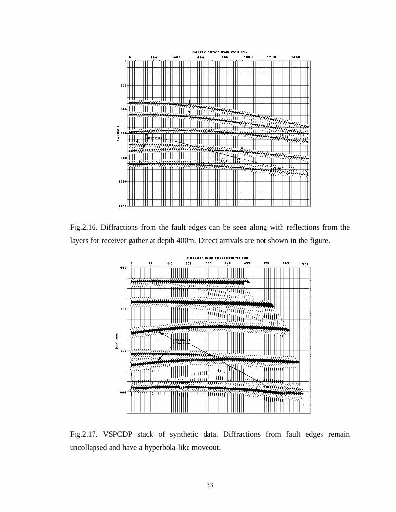
Kirchhoff diffraction modelling was used to generate synthetic P-P data for the model
shown in Figure 2.15. Five borehole receivers were placed at depths between 400-460m
every 15m. The shot interval was 15m and shot offsets from the well ranged from 5-
1500m. Diffractions from the fault edges at A, C and D can be seen on the receiver
gathers (Figure 2.16). Diffractions from zone B are not visible as they interfere with
reflection arrivals from the reflector at about 1600m depth. A VSPCDP stack from the
entire dataset was obtained following the procedure outlined in the previous sections
(Figure 2.17). One can observe that diffractions also stack and have a hyperbola-like
moveout. A post-stack Kirchhoff migration was then applied to the VSPCDP stacked

32
data using moveout velocities obtained from receiver gather at 430m depth (Figure 2.18).
The post-stack migration has significantly collapsed the diffractions and the fault edge is
more visible. Due to the robustness of post-stack time migrations, varying the velocities
by 10% did not result in significant change in the final migrated section shown in the
figure. Comparing the result with raytracing reflections in Figure 2.19, one could infer
that post-stack migration did not correctly position the reflections. This is expected as the
above process is a further approximation to the normal application of post-stack
migrations to surface seismic data.
Fig.2.15. Model used for generating synthetic data by Kirchhoff diffraction modelling.
33
Fig.2.16. Diffractions from the fault edges can be seen along with reflections from the
layers for receiver gather at depth 400m. Direct arrivals are not shown in the figure.
Fig.2.17. VSPCDP stack of synthetic data. Diffractions from fault edges remain
uncollapsed and have a hyperbola-like moveout.

34
Fig.2.18. VSPCDP stacked data in Figure 2.16 after post-stack Kirchhoff migration.
Fig.2.19. Raytracing showing specular reflections from the layer at 1200m depth.

35
2.6 Conclusions
The traveltime-offset relation for reflections recorded in the VSP geometry can be
approximated by a hyperbola. This relation provides a statistical framework to NMO
correct VSP data in the receiver domain by using amplitude semblance analysis. The
method is robust and accurately corrects VSP data to normal incidence time for a
horizontally layered earth. Moveout correction using semblance analysis is easier to use
compared to raytracing especially in the 3-D context where the data volume is large.
VSPCDP mapping of P-wave arrivals based on an approximate mapping method gives
reasonably accurate reflection maps when compared to the raytracing method. However,
raytracing is the preferred option when mapping converted-wave reflections.
Post-stack migration of VSPCDP stacked data, although theoretically incorrect, could be
used keeping in mind the approximations and limitations of such a process. In simple
geology, VSPCDP stack followed by post-stack migration may suffice to give a
reasonably accurate picture of the geology around the borehole.
The methods developed for VSP acquisition are an efficient way to obtain 2-D or 3-D
seismic images in simple geology. In complex geology, however, they could precede
more accurate imaging methods like pre-stack depth migration to give additional
information about the geology.

36
CHAPTER 3: 3C-3D VSP IMAGING: THE BLACKFOOT EXPERIMENT
3.1 Introduction
As discussed in Chapter 1 and from Stewart and Gulati (1997), we know that borehole
seismic surveys have a long history of providing rock properties such as interval velocity,
impedance and attenuation near the borehole. These surveys have also assisted surface-
seismic interpretation through time-to-depth values and the provision of a zero-phase
reflectivity that is largely multiple-free. These results are basically one-dimensional
within a Fresnel zone near the borehole.
With the advent of offset source positions, techniques were developed to obtain a
structural image from VSP data (Wyatt and Wyatt, 1984; Chang and McMechan, 1986,
Whitmore and Lines, 1986). These produced credible 2-D sections. While valuable, this
2-D VSP image still had limitations such as suffering from restricted angular coverage
per bin, limited total bin fold, and difficulty tying various shot statics and moveout.
The fundamental 2-D limitation in a VSP, and indeed many of the other previously
mentioned problems, can be overcome by using an areal distribution of shot points, or in
the reverse VSP case an areal distribution of receivers. This allows a 3-D image to be
constructed near the borehole.
Interest in 3-D well seismic data led to investigations of the feasibility and advantages of
using the 3-D VSP geometry. Chen and McMechan (1992) used a pre-stack depth
37
migration algorithm and synthetic 3-D reverse VSP data to investigate imaging of salt
structures. They found that 3-D imaging provided imaging of dips and structures not
normally accessible to surface surveys. Sun and Stewart (1994) used raytracing over a
dome model in a synthetic 3-D reverse VSP and found that converted-waves provided
significant coverage of the dome compared to compressional waves. Clochard et al.
(1997) used pre-stack migrations and showed the ability of 3-D VSP to image complex
structures.
Early 3-D VSP surveys included those conducted by AGIP in 1986 in Brenda field and
the 1989 Ekofisk 3-D VSP by Phillips Petroleum group of companies (Dangerfield,
1996). Subsequent to these, several more 3-D VSPs have been shot. Shekhtman et al.
(1993) outlined a land VSP where they used vibrators over an area and a 3-level VSP tool
to construct a 3-D image. Shell, UK shot a 3-D VSP over the Brent field, North Sea in
1993 for optimizing the development of the field (Van der Pal et al., 1996). The Ekofisk
reservoir was revisited and more 3-D VSPs were shot over the field (Farmer et al., 1997;
Omnes and Clough, 1998). Fairborn and Harding, Jr. (1996) showed a case in Louisiana
of using a downhole vibratory source and a surface spread of receivers to reconstruct a 3-
D tomographic image of a sinkhole. A CREWES-supported group shot a 3-D VSP over
the Blackfoot field in 1995 simultaneously with a surface 3C-3D survey. The main goal
was to assess the 3-D VSP capability for improved delineation of a Glauconitic sand-
channel (Stewart and Zhang, 1996). Recently, a 3-D VSP was shot over BP’s Magnus
field to improve structural interpretation of the field (First Break, 1997).

38
Several authors have analysed 3-D VSP data processing. Sun and Stewart (1994)
proposed a processing flow that included common receiver and common shot gathering,
statics removal, binning, and pre-stack migration. Boelle et al. (1998) describe the whole
processing sequence used for processing the Oseberg 3-D VSP data. Zhang et al. (1997)
developed rapid moveout correction and VSPCDP mapping methods to process the
Blackfoot 3-D VSP survey. Chen (1998), and Chen and Peron (1998) implemented the
ray-trace mapping method using 3-D velocity models and applied it to real data. Farmer
et al. (1997) used a 3-D tomographic inversion scheme for determining velocities in the
depth migration of a 3-D VSP survey over the Ekofisk field. Mittet et al. (1997) used a 3-
D elastic reverse time migration scheme and applied it to synthetic and the Oseberg 3C-
3D VSP circular shoot. Clochard et al. (1998) showed that elastic depth migration of the
Oseberg VSP data with no wavefield separation gave interpretable images consistent with
those obtained after wavefield separation. Bicquart (1998) applied Kirchhoff depth
migration to two real data examples and obtained images comparable with those from
surface 3-D seismic data.
Standard 3-D seismic interpretive techniques have also been applied to the 3-D volume
obtained from the 3-D VSP surveys. The 1989 Ekofisk 3-D VSP resulted in a clear image
where the surface 3-D had failed (Dangerfield, 1996). The Brent 3-D VSP revealed fault
patterns that were more complex and better resolved compared to those from the surface
seismic (Van der Pal et al., 1996). Results from an initial 3-D VSP processing flow over
the Blackfoot field resulted in an image consistent with that of a 3-D surface seismic
survey in the area (Zhang et al., 1997). Farmer et al. (1997) indicate that processing of a
39
later 3-D VSP survey over the Ekofisk field resulted in a vastly improved image of the
Ekofisk reservoir. Boelle et al. (1998) observed that the 3-D borehole seismic gave more
details within the reservoir formation compared to the surface seismic. These results
show the promise of the 3-D VSP and are nicely summarized by Dangerfield’s (1996)
statement:
“3-D borehole profiles should be considered as a working alternative to 2-D
borehole profiles since the extra rig time and cost are surprisingly small and the
benefits of 3-D are substantial”.
In this chapter, results from the Blackfoot 3C-3D VSP are presented. Initial results from
the Blackfoot survey were first presented by Zhang et al. (1997). Since then
developments in the processing flow have resulted in an improved image of the channel
body in the area and new results presented in this chapter. The following sections give
details of the survey from the acquisition to the interpretation stage.
3.2 Acquisition of the Blackfoot 3C-3D VSP
In 1995, a 3C-3D VSP survey was conducted by the CREWES Project by recording an
existing 3C-3D surface survey over the Blackfoot field. The Blackfoot field, which is
owned by PanCanadian Petroleum Ltd., is located about 15 kilometres southeast of
Strathmore in Alberta, Canada. The producing formation within the Blackfoot area is a
Lower Cretaceous, cemented glauconitic sand. The sand was deposited as incised
channel-fill sediments above Mississippian carbonates (Wood and Hopkins, 1992). The
40
glauconitic sandstone lies at a depth of about 1,500m below surface and is up to 45m
thick. The average porosity in this producing sandstone is near 18% and the cumulative
production from it throughout southern Alberta exceeds 200 million barrels of oil and
400 BCF gas (Margrave et al., 1998).
The simultaneous monitoring of shots used in the surface 3C-3D program enabled very
cost-effective acquisition of the 3-D VSP survey. The objectives of the survey were (i) to
see if it was logistically possible, (ii) to develop acquisition and processing procedures
for 3-D VSP, and (iii) to determine if the 3-D VSP data could image the channel body.
The downhole recording of the surface shots was acquired in well 100/12-16-023-23W4
(Figure 3.1) using Baker Atlas’s 5-level receiver tool. The 3-D VSP recorded 431 source
locations, 4 kg. of dynamite in 18 m holes arranged in 12 lines. The 12 north-south shot
lines for the 3-D VSP were spaced 210 m apart with a shot interval of 60 m. Only the
shots within 2200 m offset from the well were used out of the total 1395 sources acquired
in the whole 3C-3D survey. The shot parameters were designed to meet the criteria of the
surface survey and were not optimized for the 3-D VSP survey.
Zhang et al. (1997) indicate that it was intended to have the receiver tool deep in the well
for near-offset shots to obtain high-resolution coverage of the target near the borehole
and good velocity control. The tool would then be moved progressively shallower for far-
offset shots to obtain wider sub-surface coverage.
41
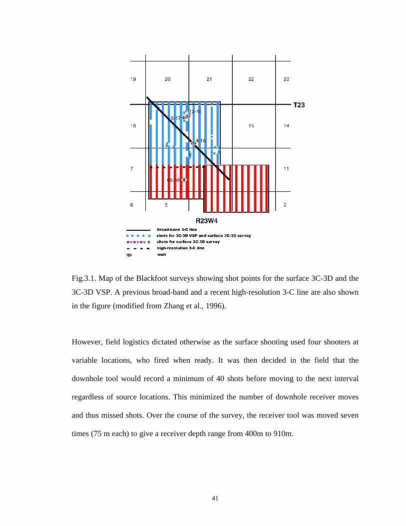
Fig.3.1. Map of the Blackfoot surveys showing shot points for the surface 3C-3D and the
3C-3D VSP. A previous broad-band and a recent high-resolution 3-C line are also shown
in the figure (modified from Zhang et al., 1996).
However, field logistics dictated otherwise as the surface shooting used four shooters at
variable locations, who fired when ready. It was then decided in the field that the
downhole tool would record a minimum of 40 shots before moving to the next interval
regardless of source locations. This minimized the number of downhole receiver moves
and thus missed shots. Over the course of the survey, the receiver tool was moved seven
times (75 m each) to give a receiver depth range from 400m to 910m.

42
3.3 Processing the 3C-3D VSP data
Initial analysis and processing of the raw data was first performed by Zhang et al. (1996).
The results from an improved processing flow are presented here. The first objective of
processing the data was to separate the upgoing compressional and shear wavefields. This
was followed by mapping of the upgoing P-waves and converted-waves to obtain 3-D
images from the survey.
3.3.1 Upgoing compressional and shear wavefield separation
The data were processed by Baker Atlas to obtain the upgoing compressional and shear
wavefields. Although the data volume for the entire 3-D VSP survey was small (about
2000 traces per component), processing the data with conventional VSP wavefield
separation techniques posed new challenges. Wavefield separation and VSP
deconvolution had to be applied with care in lieu of having only 5 levels of receivers for
each shot. Figure 3.2 outlines the steps followed by Baker Atlas in processing the raw
data to separate the two upgoing wavefields, and is discussed in the following sections.
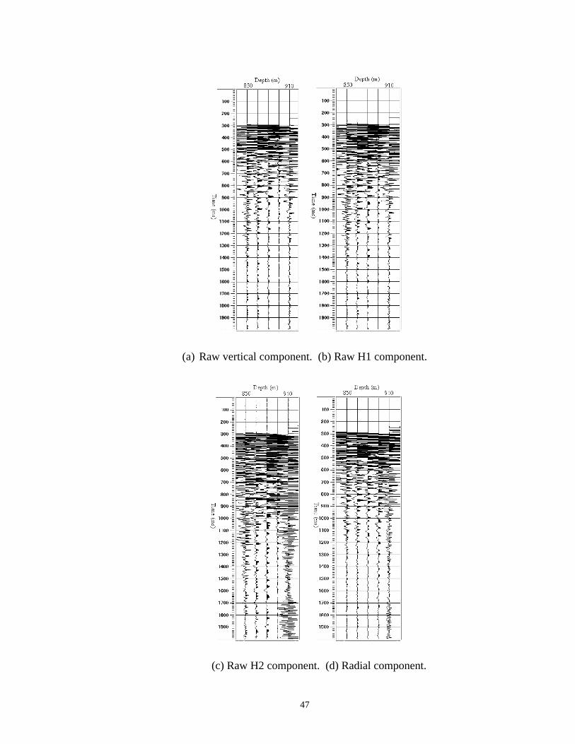
Figures 3.3a-3.3c show the raw shot gathers for shot at an offset of 372m from the well.
Apart from the direct arrivals, it is very difficult to see any events on these gathers. The
coupling resonance is seen to be stronger on the two horizontal components compared to
the vertical component. This indicates that the VSP sonde carrying the three-component
geophones is well coupled vertically but not horizontally for the receiver depths shown in
the figures.

43
After geometry and trace edits, shot statics from the surface 3-D survey were applied to
the three-component VSP data. This was followed by hodogram analysis of the two
horizontal components (here referred to as H1 and H2) in a small window around the
direct arrivals. Hodogram analysis was used to align one of the horizontal components in
the direction of the source. The horizontal component aligned in the direction of the
source is henceforth referred to as the radial component and the other as the transverse
component. Figure 3.3d is the radial component data obtained after hodogram analysis of
the H1 and H2 shots gathers of Figures 3.3b and 3.3c respectively. It is interesting to note
that the presence of casing resonance is weaker on 910m receiver on the radial
component than on the corresponding H2 component. A downgoing wave at about 880ms
is also decipherable on the radial component.
The same exponential gain correction was applied to both the vertical and radial
component data. The two datasets were time-shifted using first-break arrival times to
align downgoing P-waves on both of them. A small median filter of seven traces was then
used to separate downgoing P-waves from the data. Next, downgoing converted-waves
were separated from the data by using a median filter based on the moveout of the
downgoing converted-wave. Figures 3.3e-3.3f show the resultant downgoing and upgoing
compressional and shear wavefields. Although downgoing and upgoing events are now
visible, wavefield separation has also resulted in upgoing energy leaking onto the
downgoing part of the wavefield. Nonetheless, the results are satisfactory considering
that there were only five receiver depths for each shot location. Use of a modal filter

44
(Esmersoy, 1990; Labonte, 1990) would probably give better results than those shown in
Figure 3.3.
Upgoing converted-waves and P-waves were then removed from the vertical and radial
component data respectively by using a three-trace median filter based on the moveout of
the downgoing P-waves. This was followed by a trace-by-trace VSP deconvolution
(Kennett et al., 1980) based on the downgoing P-waves in a window of 180ms around the
first-breaks to give the P-wave and converted-wave reflectivity traces (Figure 3.4).
From the shot gathers in Figure 3.4, we observe that data on the radial component has
larger moveout compared to that on the vertical component data, thereby, indicating
effective wavefield separation. The process of obtaining upgoing P-wave and converted-
wave reflections was carried out either on a trace-by-trace basis or in shot gathers. So in
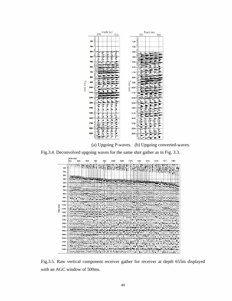
this context, it is important to verify the results by making some observations on receiver
gathers of the data (Figures 3.5-3.7). As the data on each component is a superposition of
several wavefields, the receiver gathers in general look noisy. Nonetheless, several events
can be seen on both the raw vertical component and one of the horizontal components of
the data (Figures 3.5 and 3.6). The H2 horizontal component (Figure 3.7) appears to be
mainly dominated by noise. The upgoing deconvolved P-wave and converted-wave
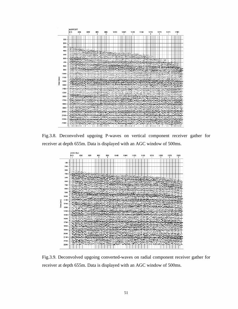
reflections are shown in Figures 3.8 and 3.9 respectively. The reflection signals are strong
on both the vertical and radial component receiver gathers. The results of processing the
data are more evident on the radial component data. In Figures 3.6 and 3.7, the raw
horizontal components lack regular moveout of events. On the contrary, the radial
45
component in Figure 3.9 shows regular moveout of events. Also, events on the radial
component data have larger moveout with offsets when compared to the vertical
component data. These observations increase confidence about the processing results.
3.3.2 P-wave and converted-wave 3-D imaging
The deconvolved upgoing P-wave and converted-wave reflections were then used to
generate 3-D volumes. Equation 2.13 and the velocity model in Figure 2.3 were first used
to calculate the fold distribution for the P-wave at the target depth of 1500m for different
bin configurations. A bin size of 110m by 20m was then decided upon as the smallest bin
size that gave uniform fold distribution at the target depth (Figure 3.11). Due to the
sparse data of about 2000 traces and reflection coverage of about a square km. at the
target depth, the average fold per bin location was a small number. Moreover, although
the bin size of 110m by 20m resulted in uniform fold distribution, the azimuth and offset
coverage in each bin was somewhat variable. This was unavoidable due to the manner in
which shots for the 3-D VSP survey were undertaken and also due to the recording taking
place only in one well location.

46
Fig.3.2. Processing flow to obtain deconvolved upgoing P-wave and converted-waves
from the 3C-3D VSP data.
47
(a) Raw vertical component. (b) Raw H1 component.
(c) Raw H2 component. (d) Radial component.

48
(e) Downgoing P-waves. (f) Downgoing converted-waves.
(f) Upgoing P-waves. (g) Upgoing converted-waves.
Fig.3.3. Shot gathers for shot at an offset of 372m from the well.
49
(a) Upgoing P-waves. (b) Upgoing converted-waves.
Fig.3.4. Deconvolved upgoing waves for the same shot gather as in Fig. 3.3.
Fig.3.5. Raw vertical component receiver gather for receiver at depth 655m displayed
with an AGC window of 500ms.

50
Fig.3.6. Raw H1 component receiver gather for receiver at depth 655m displayed with an
AGC window of 500ms.
Fig.3.7. Raw H2 component receiver gather for receiver at depth 655m displayed with an
AGC window of 500ms.
51
Fig.3.8. Deconvolved upgoing P-waves on vertical component receiver gather for
receiver at depth 655m. Data is displayed with an AGC window of 500ms.
Fig.3.9. Deconvolved upgoing converted-waves on radial component receiver gather for
receiver at depth 655m. Data is displayed with an AGC window of 500ms.
52
3.3.2.1 P-wave imaging
Two approaches were taken for the VSPCDP mapping of P-wave reflections (Figure
3.10). One approach was to use conventional raytracing and the other was to use
amplitude semblance and Equation 2.3 mapping formula as discussed in Chapter 2. The
elastic model used for the raytrace mappings is shown in Table 2.1.
The model was interactively built until traveltimes computed by raytracing through the
model matched with the observed traveltimes (John Parkin, personal communication).
Figures 3.12 and 3.13 show an inline from the VSPCDP stacks using the two mapping
methods. The two are remarkably similar except at bin locations further from the well
where the raytracing method yields more coherent reflections. This is more due to an
incomplete implementation than due to the traveltime moveout approximation of the
latter method. Figure 3.14 shows the correlation between the two results.
The stacked sections were then trace equalized followed by time-variant spectral
whitening. To interpret the stacked volumes using standard interpretive techniques, we
would require that every bin location be represented by a reflectivity value. As this was
not possible with the 3-D VSP survey at hand, f-xy deconvolution was then used to fill in
empty bin locations. F-xy deconvolution also serves to increase the coherency of
reflection events (compare Figures 3.12 and 3.15).
53
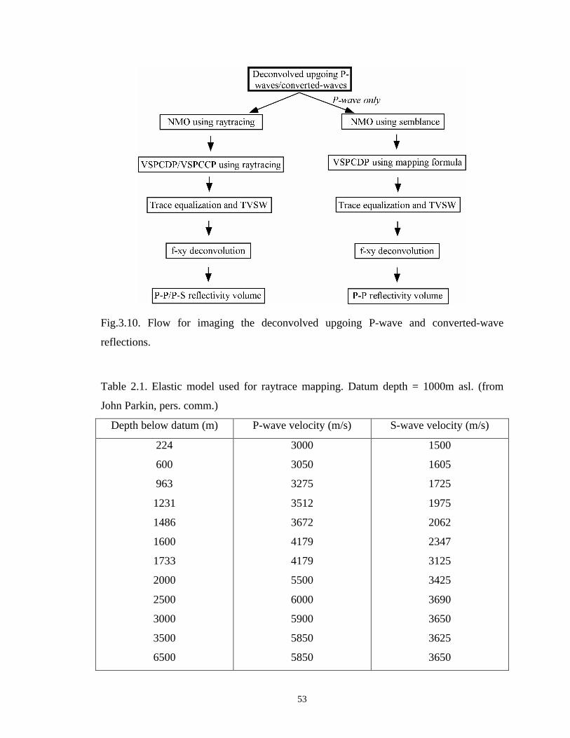
Fig.3.10. Flow for imaging the deconvolved upgoing P-wave and converted-wave
reflections.
Table 2.1. Elastic model used for raytrace mapping. Datum depth = 1000m asl. (from
John Parkin, pers. comm.)
Depth below datum (m) P-wave velocity (m/s) S-wave velocity (m/s)
224
600
963
1231
1486
1600
1733
2000
2500
3000
3500
6500
3000
3050
3275
3512
3672
4179
4179
5500
6000
5900
5850
5850
1500
1605
1725
1975
2062
2347
3125
3425
3690
3650
3625
3650
54
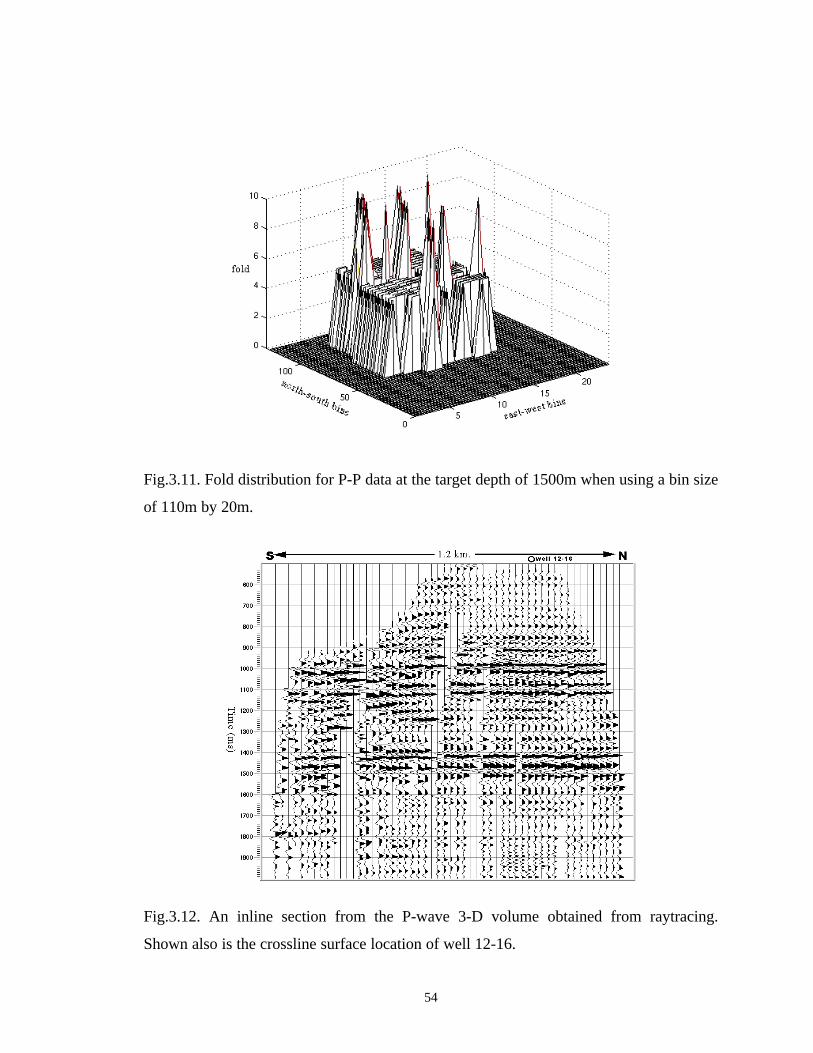
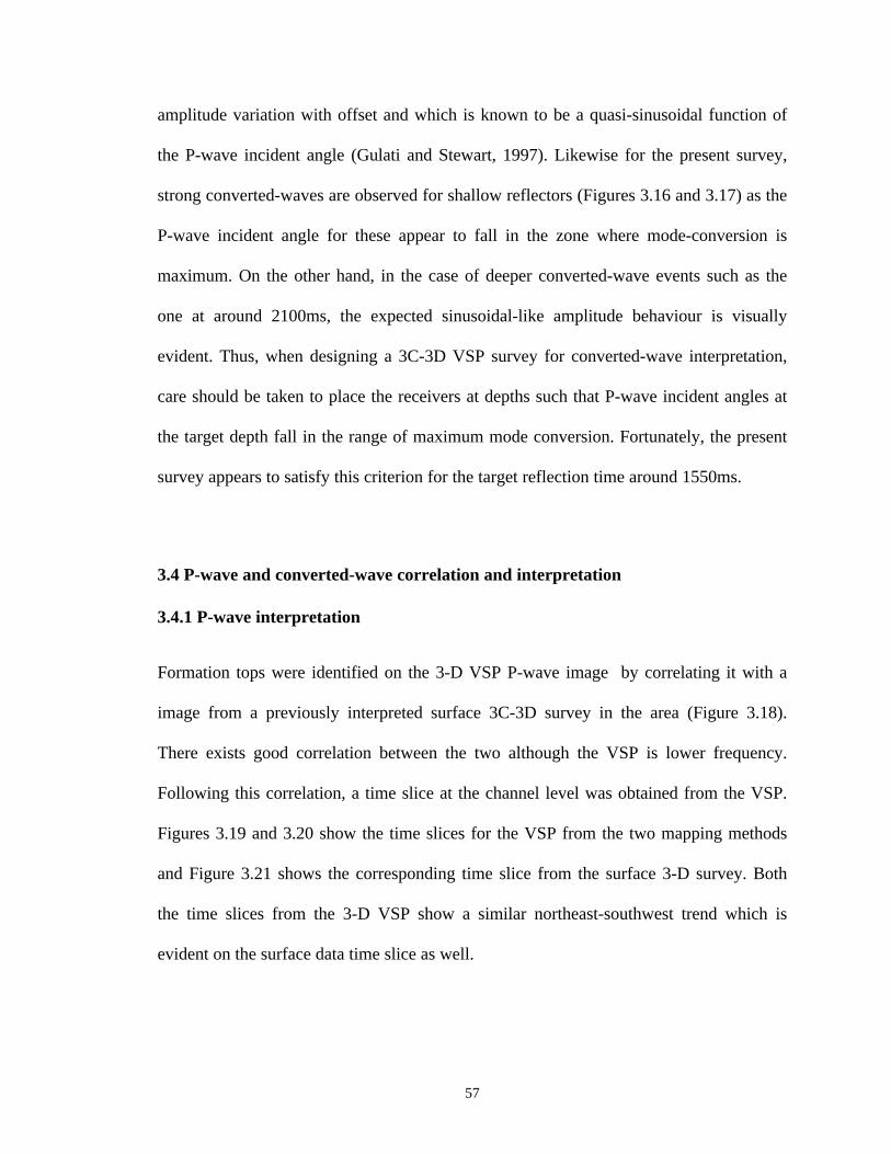
Fig.3.11. Fold distribution for P-P data at the target depth of 1500m when using a bin size
of 110m by 20m.
Fig.3.12. An inline section from the P-wave 3-D volume obtained from raytracing.
Shown also is the crossline surface location of well 12-16.

55
Fig.3.13. An inline section from the P-wave 3-D volume obtained from semblance and
mapping formula. Shown also is the crossline surface location of well 12-16.
Fig.3.14. Correlation of the 3-D VSPCDP stacking of P-wave reflections using two
different mapping methods.

56
Fig.3.15. Same inline section as in Figure 3.12 but after trace equalization, time-variant
spectral whitening and f-xy deconvolution.
3.3.2.2 Converted-wave imaging
The converted-wave reflection mapping was done using the conventional raytracing
approach only. Apart from raytracing being the preferred option for converted-wave
mapping, the approximate converted-wave mapping could not be implemented due to
technical reasons.
The radial component data was VSPCCP stacked using the same bin size of 110m by
20m as in the case of P-wave data (Figure 3.16). The stacked data was then passed
through the same processes as in the case of P-wave data to give the final interpretable
volume (Figure 3.17). Unlike P-wave data, all mode-converted events experience strong
57
amplitude variation with offset and which is known to be a quasi-sinusoidal function of
the P-wave incident angle (Gulati and Stewart, 1997). Likewise for the present survey,
strong converted-waves are observed for shallow reflectors (Figures 3.16 and 3.17) as the
P-wave incident angle for these appear to fall in the zone where mode-conversion is
maximum. On the other hand, in the case of deeper converted-wave events such as the
one at around 2100ms, the expected sinusoidal-like amplitude behaviour is visually
evident. Thus, when designing a 3C-3D VSP survey for converted-wave interpretation,
care should be taken to place the receivers at depths such that P-wave incident angles at
the target depth fall in the range of maximum mode conversion. Fortunately, the present
survey appears to satisfy this criterion for the target reflection time around 1550ms.
3.4 P-wave and converted-wave correlation and interpretation
3.4.1 P-wave interpretation
Formation tops were identified on the 3-D VSP P-wave image by correlating it with a
image from a previously interpreted surface 3C-3D survey in the area (Figure 3.18).
There exists good correlation between the two although the VSP is lower frequency.
Following this correlation, a time slice at the channel level was obtained from the VSP.
Figures 3.19 and 3.20 show the time slices for the VSP from the two mapping methods
and Figure 3.21 shows the corresponding time slice from the surface 3-D survey. Both
the time slices from the 3-D VSP show a similar northeast-southwest trend which is
evident on the surface data time slice as well.

58
Fig.3.16. An inline section from the converted-wave 3-D volume obtained from
raytracing. Shown also is the crossline surface location of well 12-16.
Fig.3.17. Same inline section as in Figure 3.16 but after trace equalization, time-variant
spectral whitening and f-xy deconvolution.
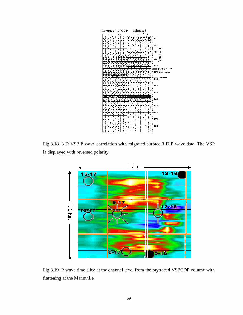
59
Fig.3.18. 3-D VSP P-wave correlation with migrated surface 3-D P-wave data. The VSP
is displayed with reversed polarity.
Fig.3.19. P-wave time slice at the channel level from the raytraced VSPCDP volume with
flattening at the Mannville.
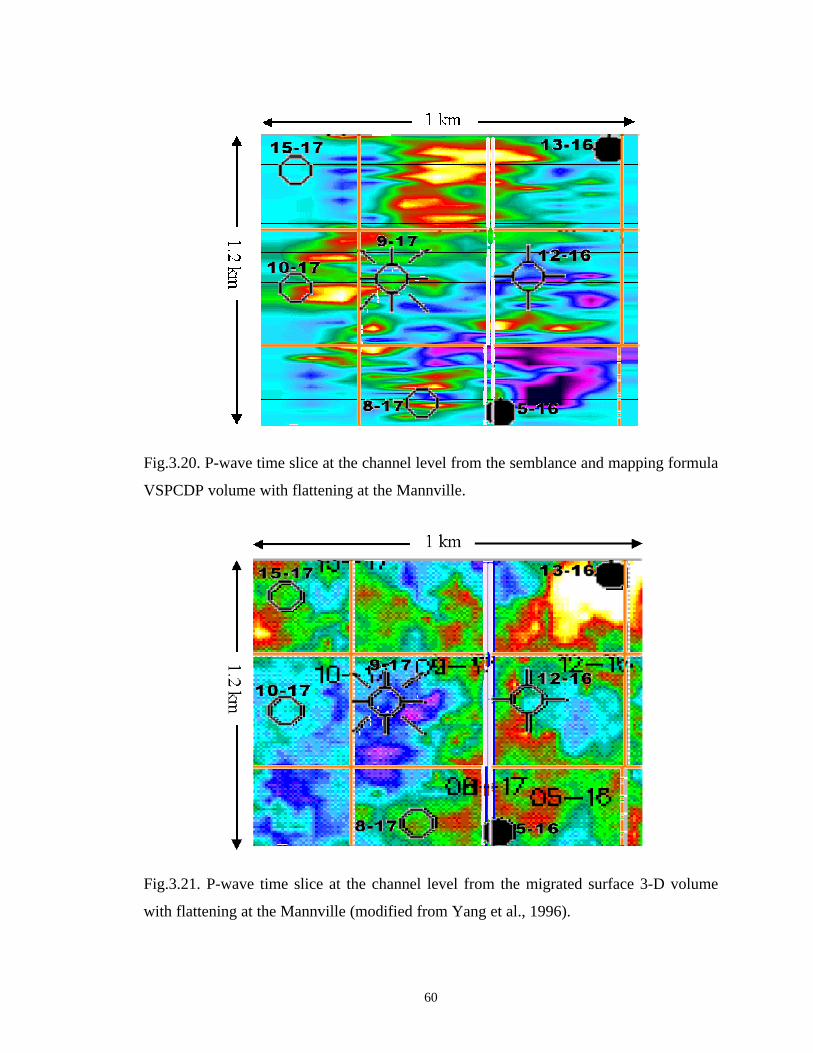
60
Fig.3.20. P-wave time slice at the channel level from the semblance and mapping formula
VSPCDP volume with flattening at the Mannville.
Fig.3.21. P-wave time slice at the channel level from the migrated surface 3-D volume
with flattening at the Mannville (modified from Yang et al., 1996).

61
Figure 3.22 shows the entire time slice from the surface 3-D survey. It shows a north-
south channel trend joined by another channel body from the west in the north-side of the
map. Figure 3.23 shows the same time slice but with the time slice from the raytraced 3-
D VSP inset into it. Comparing Figures 3.22 amd 3.23, one can observe that the channel
trend is similar in both the time slices. However, the channel in the northern part of the
map appears to have a more easterly trend in the original time slice of Figure 3.22.
3.4.2 Converted-wave interpretation
The converted-wave image from the VSP was also correlated and interpreted in a similar
manner. Formation tops were identified on the converted-wave data from the VSP by
correlating it with a previously interpreted surface 3C-3D survey in the area (Figure
3.24). In the zone of interest, the converted-wave from the VSP appears to show
somewhat better resolution than the converted-wave image from the surface seismic data.
However, at later times, the surface seismic image is higher frequency compared to the
VSP image.
In addition, the above converted-wave images were also correlated with P-wave images
from the 3-D VSP and the surface 3-D, with images from an offset 3-C VSP and with
synthetics derived from well-logs (Figure 3.25). From these correlations, the channel
anomaly on the converted-wave 3-D VSP image is seen to be a trough. Following this, a
time slice at the channel level was obtained for the converted-wave image from the 3-D
VSP (Figure 3.26). The corresponding time slice from the surface 3C-3D survey is shown
in Figure 3.27. Due to their small size, it is difficult to interpret these time slices. Figure

62
3.28 shows the converted-wave time slice from the entire 3C-3D survey and Figure 3.29
is the same time slice but with the converted-wave time slice from the 3-D VSP inset into
it. The north-south trending channel has a easterly drift in the north part of the map in
Figure 3.28. The same trend is seen in Figure 3.29 as well but the drift to the east starts
more to the south in Figure 3.29 than in Figure 3.28.
3.5 Conclusions
The Blackfoot 3-D VSP experiment has shown that acquisition of simultaneous 3-D VSP
and surface seismic surveys is possible and is cost-effective. Basic processing of the 3-D
VSP data has shown the robustness of such simultaneous acquisitions. There is also a
need for improvement in the wavefield separation and deconvolution processes and new
techniques need to be developed.
VSPCDP stacking of the 3-D VSP data using amplitude semblance analysis was observed
to yield meaningful results. While the recording geometry for the 3-D VSP was not ideal,
both P-wave and converted-wave VSP images were observed to correlate well with
images from the surface 3C-3D in the same area. Time slices from the 3-D VSP also
indicated the channel trend evident on the surface data. Results from this preliminary
survey show the promise of the 3-D VSP. The 3-D VSP could be a significant tool to
obtain high-resolution 3-D images near the borehole.
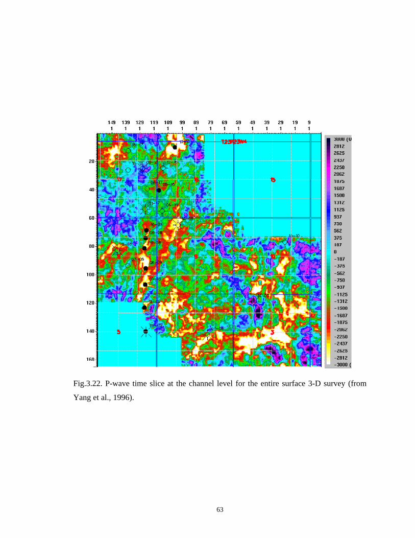
63
Fig.3.22. P-wave time slice at the channel level for the entire surface 3-D survey (from
Yang et al., 1996).
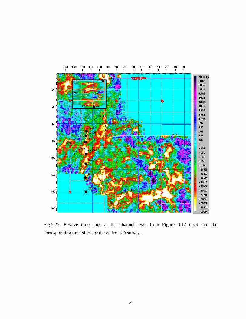
64
Fig.3.23. P-wave time slice at the channel level from Figure 3.17 inset into the
corresponding time slice for the entire 3-D survey.

65
Fig.3.24. 3-D VSP converted-wave correlation with migrated 3-D converted-wave data
from surface seismic.

66

67
Fig.3.26. Converted-wave time slice at the channel level, flattened at the Mannville, from
the 3-D VSP.
Fig.3.27. Converted-wave time slice at the channel level, flattened at the Mannville, for
the area in Figure 3.22 from the migrated surface 3-D radial data (modified from Yang et
al., 1996).
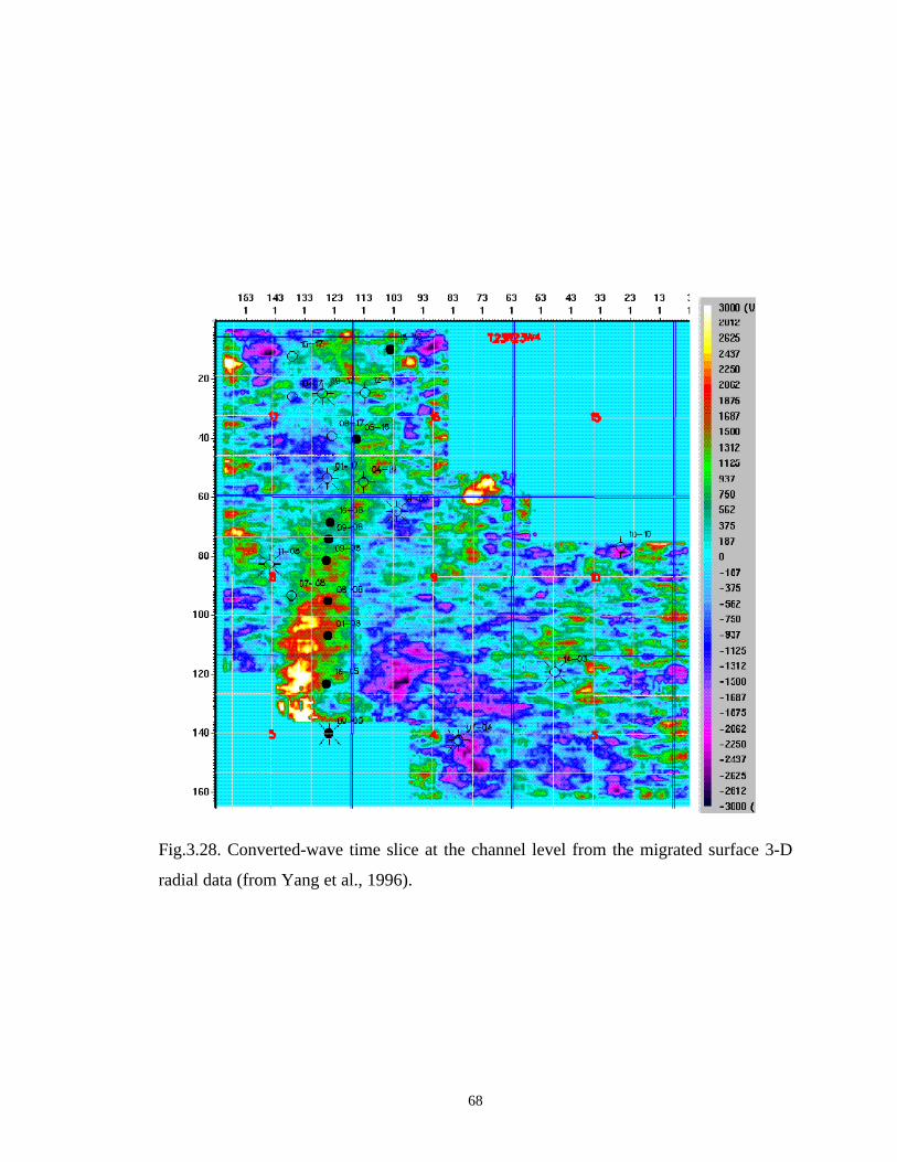
68
Fig.3.28. Converted-wave time slice at the channel level from the migrated surface 3-D
radial data (from Yang et al., 1996).

69
Fig.3.29. Converted-wave time slice at the channel level from Figure 3.22 inset into the
corresponding time slice for the entire 3-D survey.

70
CHAPTER 4: LAND VERTICAL CABLE ACQUISITION AND IMAGING
4.1 Introduction
The widespread use of vertical seismic profile (VSP) data in imaging the earth is partially
hindered by its cost. Apart from a well being required, the VSP is expensive in its present
form also due to the speed at which the data are acquired. VSP data are conventionally
acquired using downhole seismic tools containing three-component geophones clamped
to the borehole wall. Coupling the geophone to the borehole wall is critical to recording
true earth motion (Van Sandt and Levin, 1963; Wuenschel, 1976; Gaiser et. al., 1988;
Wuenschel, 1988) and is a complicated and time-consuming process in the borehole.
Another factor adding to the acquisition time is that most tools have a maximum of five
geophone levels, so the tool is usually moved over the borehole length and shot points
repeated to obtain adequate fold and offset coverage per bin location. Recently, Omnes
and Clough (1998) demonstrate the implementation of a twelve-level tool which
significantly reduced the acquisition time of the VSP surveys they conducted. This is a
welcome advance. Paulsson (1998) shows data from a 40-level receiver tool.
A less expensive alternative for the rapid and efficient acquisition of VSP data is the use
of multi-level vertical hydrophone array. Hydrophones are pressure sensitive receivers
and not required to be clamped to the borehole wall. They are, therefore, easy to deploy
in a borehole and a large number of them can be simultaneously used in the borehole.
Early experiments using hydrophone detectors in borehole were those conducted by
White and Sengbush (1953) and Riggs (1955). Recent experiments to evaluate the
capabilities of using a vertical array of hydrophones for VSP on land were carried out by
71
Marzetta et. al. (1988) and Krohn and Chen (1992). Findlay et al. (1991) and Sheline
(1998) showed the successful implementation of an offshore crosswell reflection imaging
program that used an array of hydrophone receivers. Milligan et. al. (1997) demonstrated
the viability of using a vertical hydrophone array in a walkaway VSP to image shallow
structures on land. Most authors note that a major impediment to the use of vertical
hydrophone array in a borehole has been the presence of strong coherent noise on the
VSP data in the form of tube waves. Tube waves are guided waves confined to the
borehole fluid and hydrophones are more sensitive to the tube waves compared to
properly clamped geophones (Wuenschel, 1988; Krohn and Chen, 1992).
Both field and processing methods to attenuate tube wave noise on VSP data have been
investigated by several authors. Riggs (1955) and Gal’perin (1974) observed that moving
the surface source away from the borehole significantly reduced the intensity of tube
waves. Hardage (1981) made similar observations and also found surface ground roll
sweeping across the well head to be the principal source of tube waves. Krohn and Chen
(1992) used dipole hydrophones to attenuate tube waves in field. Pham et al. (1993) and
Milligan et al. (1997) used closed-cell-foam baffles between hydrophone elements to
suppress tube waves in borehole surveys. Velocity filtering has been very effective in
isolating tube waves in the processing centre (Hardage, 1981; DiSiena et al., 1984;
Marzetta et al., 1988; Milligan et al., 1997). Median and wavelet filtering can also be
used to remove tube waves from VSP data (Schuster and Sun, 1993). Marzetta (1992)
developed an inverse borehole coupling theory to derive a tube-wave free quantity which
he called as “squeeze strain” from data recorded using hydrophones in a borehole.
72
While these field experiments are very important to the study of vertical hydrophone
cable on land, the source-offset and the depth range in these surveys was severely limited.
The use of hydrophones in VSP surveys depends on the ability to obtain reliable offset
sections or seismic volumes of size of current VSP surveys. It was to fill in some of these
gaps that the CREWES Project at the University of Calgary acquired a shallow vertical
hydrophone cable data on land in November 1997 at the Blackfoot oil field located in
Alberta, Canada. The objectives of the hydrophone VSP survey were 1) to compare
hydrophone data with nearby three-component geophone records and determine the
validity of the raw hydrophone records and 2) to see if the hydrophone cable can be used
to obtain reliable stand-alone images. The following sections give details of the Blackfoot
land vertical cable survey from the acquisition to the data analysis and interpretation
stage.
4.2 Field description and data acquisition
On November 1-2, 1997 the CREWES Project at the University of Calgary with
assistance from Boyd PetroSearch Consultants Ltd. and PanCanadian Petroleum Ltd.
recorded a high-resolution 3C-2D seismic survey at the PanCanadian-owned Blackfoot
field. The Blackfoot field is located some 50-55km east of Calgary in Alberta, Canada
(Figure 4.1). As described before, the producing formation within the Blackfoot area is a
Lower Cretaceous, cemented glauconitic sand.

73
Fig.4.1. Map showing the location of the PanCanadian Blackfoot field.
The 3C-2D survey involved the acquisition of a 3km reflection profile which consisted of
a combination of “normal-resolution” 20m and “high-resolution” 2m receiver intervals.
The shot interval employed for the entire 2D profile was 20m and shot on the half-station.
The survey also involved the simultaneous recording into 21×3 buried 3-C geophones
situated in 6, 12 and 18m holes drilled every 50m along the central km of the profile. In
addition to these buried geophones, a 48-channel vertical hydrophone cable with a 2 m
receiver interval was deployed in a 100m cased hole located in the centre of the profile
(Figure 4.2). A walk-away AVO VSP was also recorded in a well located near the centre
of the spread at the same time the surface shots were being taken.
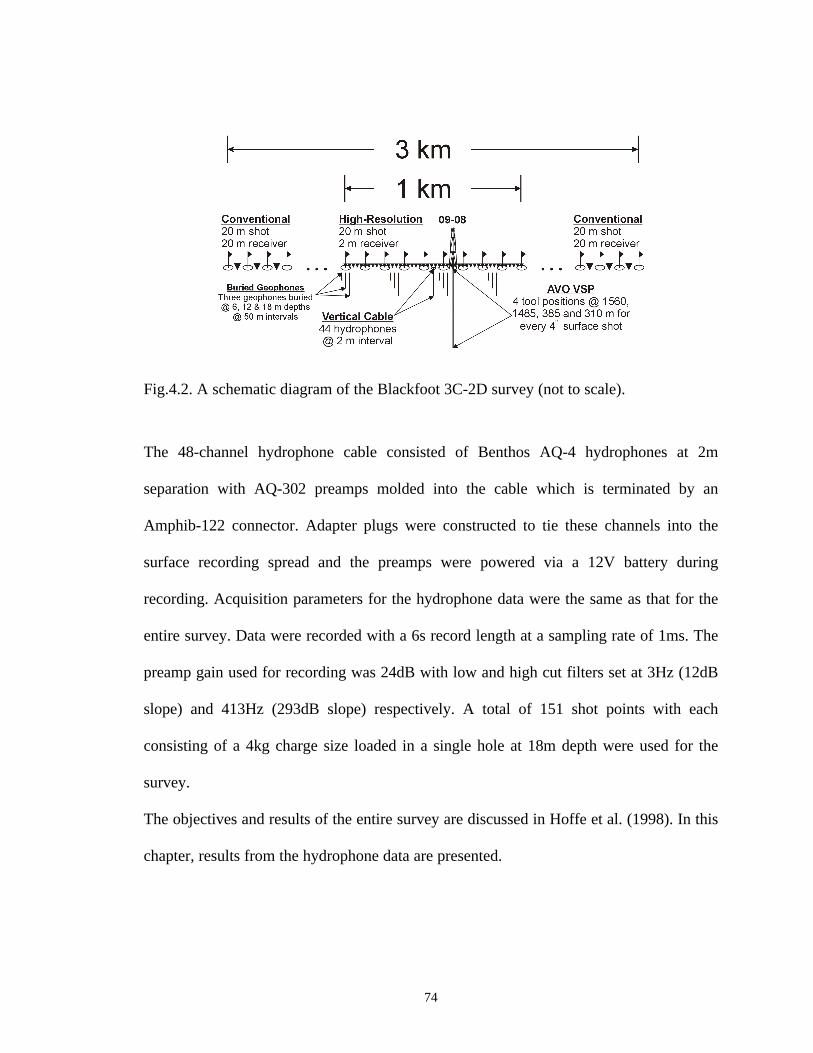
74
Fig.4.2. A schematic diagram of the Blackfoot 3C-2D survey (not to scale).
The 48-channel hydrophone cable consisted of Benthos AQ-4 hydrophones at 2m
separation with AQ-302 preamps molded into the cable which is terminated by an
Amphib-122 connector. Adapter plugs were constructed to tie these channels into the
surface recording spread and the preamps were powered via a 12V battery during
recording. Acquisition parameters for the hydrophone data were the same as that for the
entire survey. Data were recorded with a 6s record length at a sampling rate of 1ms. The
preamp gain used for recording was 24dB with low and high cut filters set at 3Hz (12dB
slope) and 413Hz (293dB slope) respectively. A total of 151 shot points with each
consisting of a 4kg charge size loaded in a single hole at 18m depth were used for the
survey.
The objectives and results of the entire survey are discussed in Hoffe et al. (1998). In this
chapter, results from the hydrophone data are presented.

75
4.3 Vertical hydrophone cable data versus geophone data
Hydrophones and geophones not only measure different physical quantities but also
record data in different physical environments. One is suspended in a fluid medium in a
borehole or in a marine environment whereas the other is clamped to a borehole-solid
interface or an air-ground interface. Properly clamped geophones are believed to portray
the true earth motion. Therefore the use of hydrophones in borehole surveys is justified if
it is known that the pressure waveform in the borehole fluid is directly related to the
stress waveform in the solid when an elastic wave passes the borehole. White (1953)
developed a “borehole coupling” theory which quantified borehole fluid pressure and
motion due to the passage of low frequency elastic waves past the hole. He observed that
the “formation break” [White (1953) defines “formation break” as the pressure signal
that has the same phase velocity as of that of the wave cutting the borehole, and which
was also called as “squeeze strain” by Marzetta (1992)] due to a compressional wave
was in phase with the disturbance in the surrounding solid. This is true when the velocity
of the wave in the solid is larger than that in the borehole fluid. Blair (1984) and
Schoenberg (1986) also made similar observations for low frequency or which is the
same as long wavelength seismic waves.
The borehole radius in which the vertical hydrophone cable was deployed was around
14cm. Using frequency filter panels, the smallest possible wavelength of the seismic data
was calculated to be 20m. The borehole geometry, therefore, satisfied the long
wavelength criterion given by Blair (1984) and the hydrophones should represent the
earth motion similar to a geophone in the surrounding solid. Thus, in theory, we expect

76
the P-wave signal on the pressure and velocity phones to be in phase assuming similar
detector transduction for both phones.
To test the validity of this hypothesis, a hydrophone receiver gather at 18m depth is
compared with a three-component geophone gather at the same depth located about 8m
away from the hydrophone. Field tap tests showed that an upcoming compressive stress
would record as a negative pulse on the geophone and a pressure increase would record
as a positive pulse on the hydrophone. We analyzed the field data considering the above
report. The first break refraction arrivals on the geophone and the hydrophone appeared
opposite polarity. On reversing the polarity of the hydrophone data, the first break
arrivals on the two phones appeared to be in phase with each other. This is in direct
agreement with White’s borehole coupling theory and increased our confidence about the
hydrophone data.
Figures 4.3-4.5 show the hydrophone data at 18m depth, the vertical and the inline
horizontal component of the geophone at the same depth respectively. One can observe
that although the hydrophone is noisy compared to the geophone gather it mimics the
refraction and reflection arrivals of the geophone data. The hydrophone data has the
character of both the vertical and inline horizontal components of the geophone. This is
because the hydrophone is sensitive to pressure generated by both the compressional and
shear wavefields. Notice also that reflections on the hydrophone data are more prominent
for shots at intermediate-to-far offsets as the ground roll arrives later in time. This
conforms well with Hardage’s (1981) observation that ground roll is the major source of
tube waves.

77
Figure 4.6 is a comparison of the amplitude spectrum of the stack of the hydrophone and
vertical component geophone gather at 18m depth. The hydrophone is seen to be lower
frequency compared to the geophone stack. Also, severe notches on the spectrum of the
hydrophone stack are representative of the tube wave interference with body wave
reflections on the hydrophone gather.
Fig.4.3. Receiver gather for hydrophone at 18m depth displayed with reversed polarity
and 250ms AGC window. SW is the zone of shear-wave refraction arrivals.

78
Fig.4.4. Receiver gather for vertical component geophone at 18m depth displayed with
normal polarity and 250ms AGC window.
Fig.4.5. Receiver gather for inline horizontal component geophone at 18m depth
displayed with normal polarity and 250ms AGC window. SW is the zone of shear-wave
refraction arrivals.
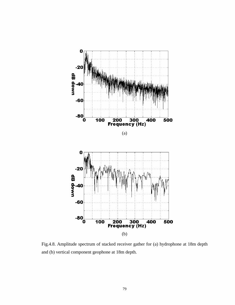
79
(a)
(b)
Fig.4.8. Amplitude spectrum of stacked receiver gather for (a) hydrophone at 18m depth
and (b) vertical component geophone at 18m depth.

80
4.5 Processing the hydrophone cable data
Tube waves are the primary source of noise present on hydrophone data acquired in
boreholes. This is true when the objective is to generate an image of the earth. The main
objective of processing the hydrophone data was, therefore, to suppress tube waves and at
the same time obtain an image that could be reliably interpreted. However, tube waves
can also be used to determine valuable information about the rigidity of the solid
surrounding the borehole as shown in White and Sengbush (1953) and Riggs (1955).
The steps involved in processing the hydrophone data (Figure 4.7) follow. After trace
edits and mutes, shot statics computed during processing of the “low-resolution” 20m
surface seismic survey were applied to the hydrophone data. Shot statics were small and
therefore application of shot statics only marginally changed the moveout of events in the
hydrophone receiver gathers (Figure 4.8). A spherical spreading gain correction using a
preliminary RMS velocity function was then applied to the data.
In the simplest case, we can assume that tube waves bounce back and forth only from the
top and bottom of the borehole. In other words, tube waves are predictable in time. The
time taken for the tube wave to travel from the top to the bottom of the borehole and back
was calculated to be around 150ms. Although an oversimplified assumption, it
nevertheless forms a basis to use predictive deconvolution. It was observed that a
predictive deconvolution operator with a 12ms prediction distance significantly
suppressed tube waves. Several reflection events that were either not visible or feebly
visible on the raw data were now be easily observed on the processed data (compare

81
Figures 4.9 and 4.10). The low-frequency and low-velocity tube waves were further
reduced by f-k filtering of shot gathers of the data (Figure 4.11). Several events at times
less than 1000ms are now clearly visible on the data. Figures 4.12-4.14 show the results
of the above processing steps for three different shot gathers. Upgoing reflection events
are much evident on the data in Figures 4.12 than in Figures 4.14. Notice a change in
character in Figure 4.12 at a depth of about 44m due to the reflection and transmission of
tube waves at that depth. Change in borehole rugosity at that depth is a likely reason for
the reflection and transmission of tube waves at that depth. This change in character is
notably absent on the processed shot gathers in Figures 4.13 and 4.14.
Velocity analysis of receiver gathers was then performed after trace equalization of the
traces. The data were then VSPCDP stacked using the procedure discussed in Chapter 2.
Several coherent reflections typical for the Blackfoot area are seen on the stacked section
(Figure 4.15). Note that a cable every 750m or so would adequately image the reservoir
at around 1000ms. Reflections on the stacked data away from the borehole show a better
continuity compared to those closer to the borehole. This is because the tube wave
contamination was stronger for shots closer to the borehole compared to shots at
intermediate-to-far offsets from the borehole. The dead traces in the section represent
missing shot locations along the profile. Time-variant spectral whitening was applied to
the stacked data which was then passed through either an f-x deconvolution or a post-
stack migration operator to give the final interpretable section.
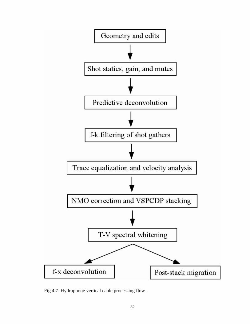
82
Fig.4.7. Hydrophone vertical cable processing flow.

83
(a) with no statics (b) with statics applied
Fig.4.8. Receiver gather for hydrophone at 98m depth.
Fig.4.9. Raw receiver gather for hydrophone at 98m depth after application of shot
statics. AGC is used for display purpose.
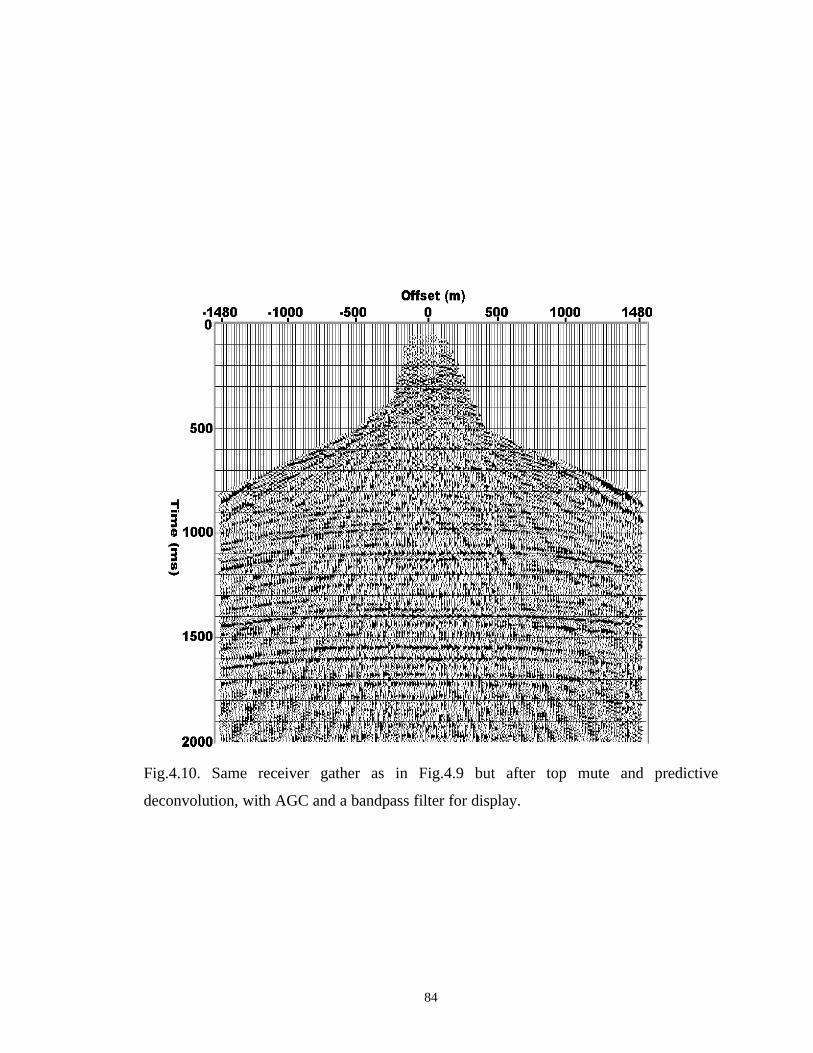
84
Fig.4.10. Same receiver gather as in Fig.4.9 but after top mute and predictive
deconvolution, with AGC and a bandpass filter for display.

85
Fig.4.11. Same receiver gather as in Fig.4.10 but after f-k filtering of shot gathers, with
AGC for display.
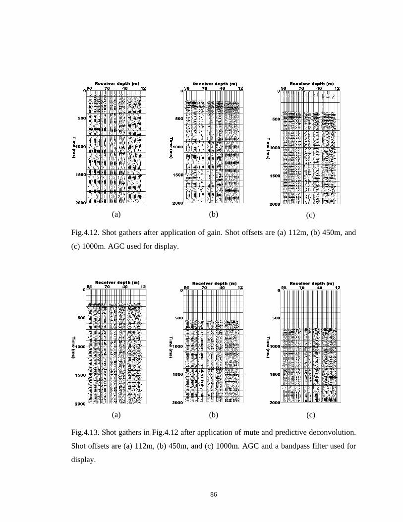
86
(a) (b) (c)
Fig.4.12. Shot gathers after application of gain. Shot offsets are (a) 112m, (b) 450m, and
(c) 1000m. AGC used for display.
(a) (b) (c)
Fig.4.13. Shot gathers in Fig.4.12 after application of mute and predictive deconvolution.
Shot offsets are (a) 112m, (b) 450m, and (c) 1000m. AGC and a bandpass filter used for
display.
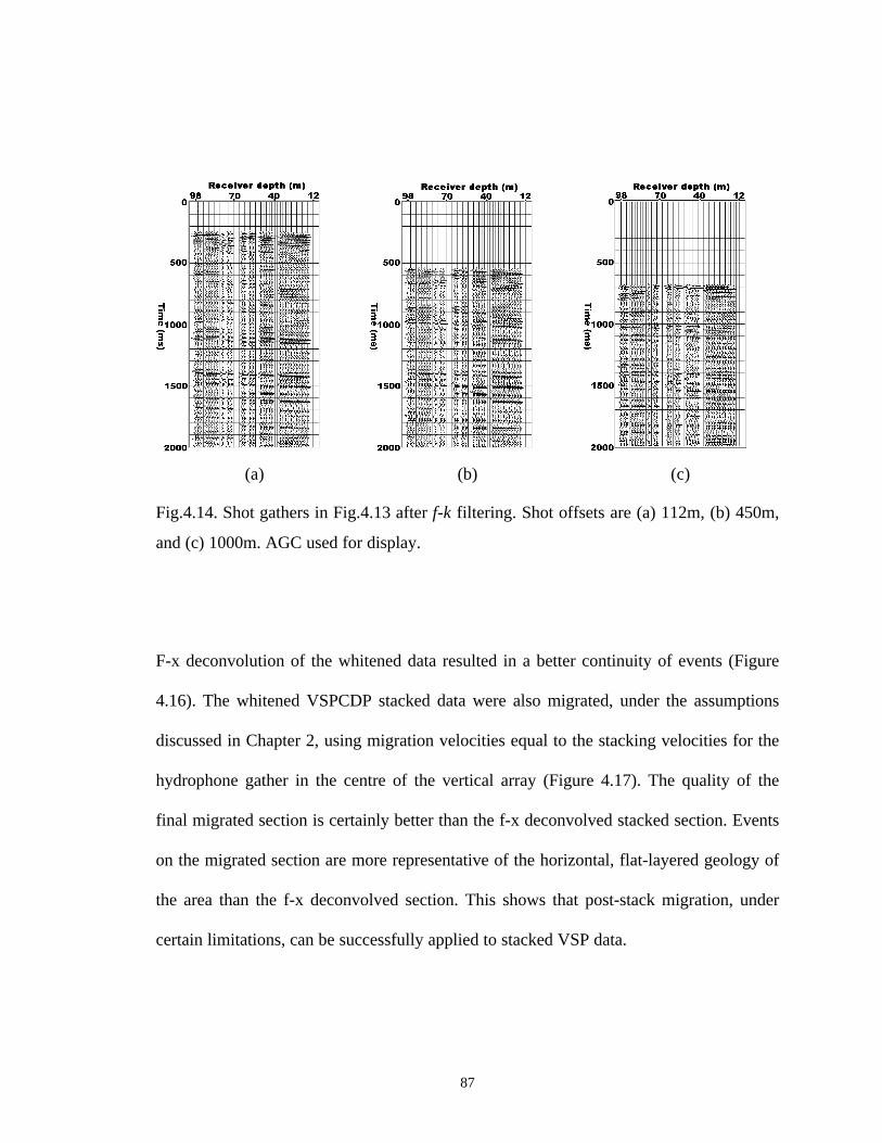
87
(a) (b) (c)
Fig.4.14. Shot gathers in Fig.4.13 after f-k filtering. Shot offsets are (a) 112m, (b) 450m,
and (c) 1000m. AGC used for display.
F-x deconvolution of the whitened data resulted in a better continuity of events (Figure
4.16). The whitened VSPCDP stacked data were also migrated, under the assumptions
discussed in Chapter 2, using migration velocities equal to the stacking velocities for the
hydrophone gather in the centre of the vertical array (Figure 4.17). The quality of the
final migrated section is certainly better than the f-x deconvolved stacked section. Events
on the migrated section are more representative of the horizontal, flat-layered geology of
the area than the f-x deconvolved section. This shows that post-stack migration, under
certain limitations, can be successfully applied to stacked VSP data.

88
Fig.4.15. VSPCDP stacked section of the hydrophone data. Trace normalization used for
display.
Fig.4.16. f-x deconvolution of the whitened VSPCDP stack in Figure 4.15.
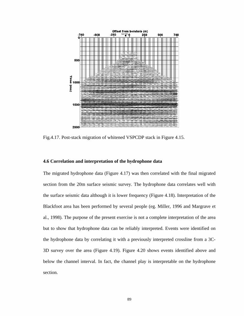
89
Fig.4.17. Post-stack migration of whitened VSPCDP stack in Figure 4.15.
4.6 Correlation and interpretation of the hydrophone data
The migrated hydrophone data (Figure 4.17) was then correlated with the final migrated
section from the 20m surface seismic survey. The hydrophone data correlates well with
the surface seismic data although it is lower frequency (Figure 4.18). Interpretation of the
Blackfoot area has been performed by several people (eg. Miller, 1996 and Margrave et
al., 1998). The purpose of the present exercise is not a complete interpretation of the area
but to show that hydrophone data can be reliably interpreted. Events were identified on
the hydrophone data by correlating it with a previously interpreted crossline from a 3C-
3D survey over the area (Figure 4.19). Figure 4.20 shows events identified above and
below the channel interval. In fact, the channel play is interpretable on the hydrophone
section.

90
Fig.4.18. Migrated hydrophone traces near the borehole spliced into a section of the final
migrated 20m surface seismic data.
Fig.4.19. Migrated hydrophone traces inserted into a previously interpreted crossline
from a 3C-3D survey in the area.
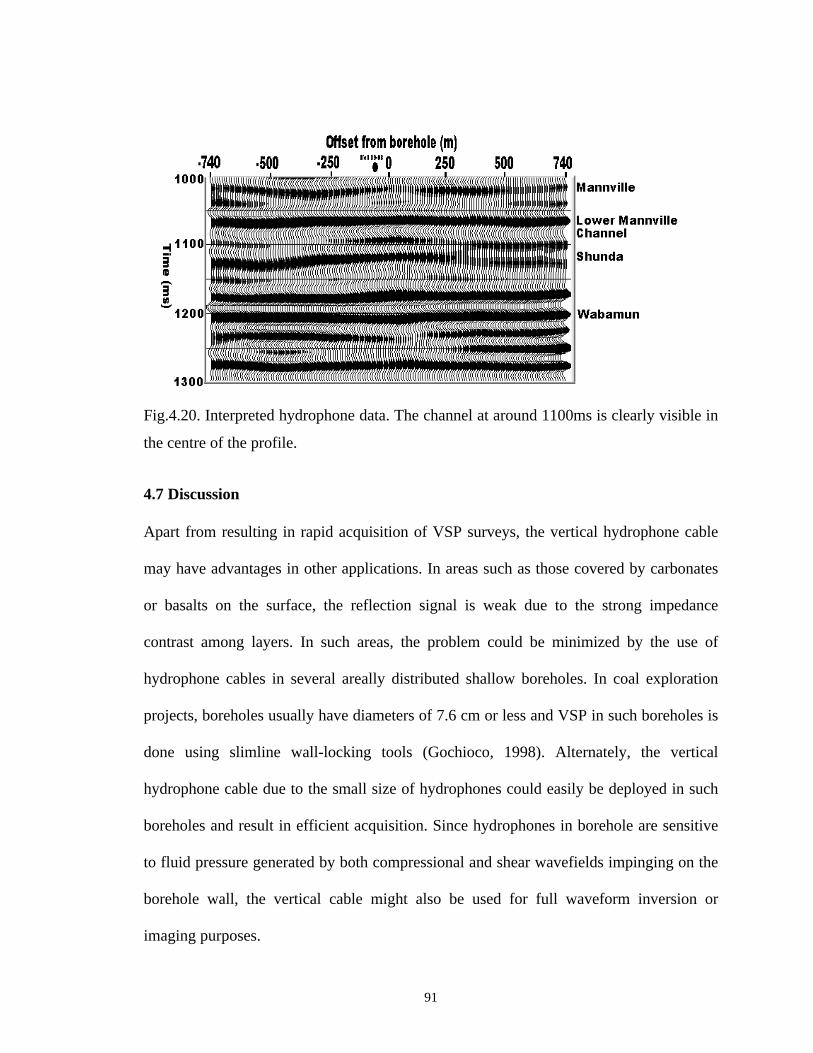
91
Fig.4.20. Interpreted hydrophone data. The channel at around 1100ms is clearly visible in
the centre of the profile.
4.7 Discussion
Apart from resulting in rapid acquisition of VSP surveys, the vertical hydrophone cable
may have advantages in other applications. In areas such as those covered by carbonates
or basalts on the surface, the reflection signal is weak due to the strong impedance
contrast among layers. In such areas, the problem could be minimized by the use of
hydrophone cables in several areally distributed shallow boreholes. In coal exploration
projects, boreholes usually have diameters of 7.6 cm or less and VSP in such boreholes is
done using slimline wall-locking tools (Gochioco, 1998). Alternately, the vertical
hydrophone cable due to the small size of hydrophones could easily be deployed in such
boreholes and result in efficient acquisition. Since hydrophones in borehole are sensitive
to fluid pressure generated by both compressional and shear wavefields impinging on the
borehole wall, the vertical cable might also be used for full waveform inversion or
imaging purposes.

92
4.8 Conclusions
Comparison of vertical hydrophone cable data with geophone data shows that in the long
wavelength case, as predicted by theory (White, 1953), hydrophones in borehole
represent the true earth motion. Tube wave contamination of hydrophone records is
severe at short offsets and decreases with increasing offset. This property of increasing
signal-to-noise ratio with increasing offset is very similar to that observed so commonly
on ground roll affected geophone data.
In the simplest case, tube waves can be assumed to be predictable in time assuming that
they bounce back and forth only from the top and bottom of the borehole. A predictive
deconvolution operator used to suppress tube wave contamination on the hydrophone
data was found to be very effective.
Processing of the vertical hydrophone cable data resulted in an image that correlated well
with that from the 20m surface seismic survey and a previous 3-D seismic survey over
the area. Events present on the surface geophone data were identifiable on the
hydrophone data as well. In fact, the channel structure was very much interpretable on the
hydrophone image. These correlations and interpretations indicate that hydrophones in
boreholes would result not only in efficient acquisition of VSP data but also result in
images that can be interpreted.

93
CHAPTER 5: CONCLUSIONS AND FUTURE WORK
5.1 Thesis conclusions
An approximate method for VSPCDP mapping of P-wave arrivals is developed for
efficient imaging of large VSP data. The method, based on amplitude semblance analysis,
is found to be robust and efficient. It gives reasonably accurate reflection maps when
compared to the raytrace VSPCDP mapping method. It is also found that post-stack
migration of VSPCDP stacked data, although theoretically incorrect, could be used under
certain limitations.
The simultaneous acquisition of the Blackfoot 3-D VSP along with a surface 3-D
program has shown that such surveys are possible and cost-effective. Both P-wave and
converted-wave images from the 3-D VSP were observed to have good correlation with
images from the surface 3C-3D survey. Time slices from the 3-D VSP inset into the
surface seismic time slices also indicated the channel trend of the Blackfoot field.
Although much work needs to be done to improve processing of the 3-D VSP data,
results from this experimental survey were encouraging and showed the potential of the
3-D VSP. The 3-D VSP could be a significant tool to obtain detailed 3-D reservoir
information near the well.
The Blackfoot land vertical cable data showed the promise of using hydrophones for
acquiring VSP data. Tube waves, which were the primary source of coherent noise on the
data, were effectively suppressed by a combination of predictive deconvolution and f-k
velocity operators. The image from the land vertical cable data correlated very well with
94
that from a 20m 2-D surface seismic data and a previous 3-D seismic data from the same
area. The channel structure in the Blackfoot field was very much interpretable on the
hydrophone image. These results show that hydrophones in borehole can not only result
in efficient acquisition of VSP but also result in images that can be interpreted.
5.2 Future work In view of most 3-D VSP surveys having few receiver levels (about 5 in most cases),
accurate wavefield separation of VSP data remains the major concern in processing the 3-
D VSP data. Wavefield separation techniques based on the Radon transform are well
documented in the literature and such techniques could be tested on the Blackfoot 3-D
VSP data for improved images. Also, accuracy of median-based technique may be
improved by applying it on offset-sorted data that has been moved to zero-offset direct
and reflection arrival times.
With increasingly large offsets in 3-D VSP data, VSP deconvolution may be
inappropriate due to the first-break arrivals not being the direct arrivals. In such cases,
statistical techniques such as surface-consistent deconvolution may be more appropriate.
Statics is another aspect of the 3-D VSP processing flow that has room for improvement.
It may be possible to develop a ray parameter approach using the polarization of the VSP
data to solve the statics problem.

95
The land vertical cable data could also be processed for generating converted-wave
images.
96
REFERENCES
Al-Chalabi, M., 1973, Series approximation in velocity and traveltime computations:
Geophysical Prospecting, 21, 783-795.
Bicquart, P., 1998, Application of Kirchhoff migration to 3D-VSP: Presented at 68th
Ann. Intl. SEG Mtg., Expand. Abst., 389-392.
Blair, D.P., 1984, Rise times of attenuated seismic pulses detected in both empty and
fluid-filled cylindrical boreholes: Geophysics, 49, 398-410.
Boelle, J., Kiaser, P. and Maocec, E., 1998, Difficulties and clues in 3D VSP processing:
Presented at 68th Ann. Intl. SEG Mtg., Expand. Abst., 373-376.
Byun, B.S., Corrigan, D. and Gaiser, J.E., 1989, Anisotropic velocity analysis for
lithology discrimination: Geophysics, 54, 1564-1574.
Chang, W. and McMechan, G.A., 1986, Reverse-time migration of offset vertical seismic
profiling data using he excitation-time imaging condition: Geophysics, 51, 67-84.
Chen, G., 1998, 3D VSP CDP mapping with interactive reflection traveltime display:
Presented at 68th Ann. Intl. SEG Mtg., Expand. Abst., 361-364.
Chen, H. and McMechan, G.A., 1992, 3-D pre-stack depth migration for salt and sub-salt
structures using reverse-VSP data: J. Seis. Explor., 281-291.
Chen, G. and Peron, J.F., 1998, Mapping of 3D VSP data using quick ray tracing:
Presented at 68th Ann. Intl. SEG Mtg., Expand. Abst., 365-368.
Clochard, V., Compte, P., Nicoletis, L., Lucas-Svay, J. and Dillon, P.B., 1997, 3D walk-
away imaging in the overthrust model: Presented at the 57th Ann. EAGE Mtg.,
E047.
97
Clochard, V., Nicoletis, L., Svay-Lucas, J., Mendes, M. and Anjos, L., 1998, 3-C
imaging of 3D walk-away data in regard to preprocessing: Presented at 68th Ann.
Intl. SEG Mtg., Expand. Abst., 377-380.
Dangerfield, 1996, Shallow 3-D seismic and a 3-D borehole profile at Ekofisk field, in
Ed. Brown, A., Interpretation of three-dimensional seismic data, AAPG Memoir
42.
DiSiena, J.P., Byun, B.S., Fix, J.E., and Gaiser, J.E., 1984, F-K analysis and tube wave
filtering, in Eds. Toksoz, N.M. and Stewart, R.R., Vertical Seismic Profiling,
Part B-Advanced Concepts, Geophys. Press.
Dillon, P.B. and Thomson, R.C., 1984, Offset source VSP surveys and their image
construction: Geophysical Prospecting, 32, 790-811.
Dix, C.H., 1955, Seismic velocities from surface measurements: Geophysics, 20, 68-86.
Esmersoy, C., 1990, Inversion of P and SV waves from multicomponent offset vertical
seismic profiles: Geophysics, 55, 39-50.
Fairborn, J.W. and Harding, R.S., Jr., 1996, 3D seismic velocity tomography at SPR
sinkhole site, Weeks Island, Louisiana: Presented at 59th Ann. Intl. SEG Mtg.,
Expand. Abst., 896-898.
Farmer, P., Chapman, C., Fryer, A., Paul, A. and Sandvin, O., 1997, 3-D tomographic
inversion and depth migration of VSP data. Presented at 60th Ann. Intl. SEG
Mtg., Expand. Abst.
Findlay, M.J., Goulty, N.R., and Kragh, J.E., 1991, The crosshole seismic reflection
method in opencast coal exploration: First Break, 9, 509-514.

98
First Break, 1997, Large 3D VSP survey completed on BP Magnus field: First Break,
15, 290.
Gaiser, J.E., Fulp, T.J., Petermann, S.G., and Karner, G.M., 1988, Vertical seismic profile
sonde coupling: Geophysics, 53, 206-214.
Gal'perin, 1974, Vertical seismic profiling, Ed. White, J.E., SEG.
Gochioco, L.M., 1998, Shallow VSP work in the U.S. Appalachian coal basin:
Geophysics, 63, 795-799.
Gulati, J.S. and Stewart, R.R., 1997, Seismic exploration through high-velocity layers:
Presented at 67th Ann. Intl. SEG Mtg., Expand. Abst., 1297-1300.
Hardage, B.A., 1981, An examination of tube wave noise in vertical seismic profiling
data: Geophysics, 46, 892-903.
Hardage, B.A., 1983, Vertical seismic profiling: Geophysical Press.
Hardage, B.A., 1992, Crosswell seismology and reverse VSP: Geophysical Press.
Hoffe, B.H., Stewart, R.R., Bland, H.C., Gallant, E.V., and Bertram, M.B., 1998, The
Blackfoot high-resolution 3-C seismic survey: design and initial results, Presented
at 68th Ann. Intl. SEG Mtg., Expand. Abst., 103-106.
Kennett, P., Ireson, R.L., and Conn, P.J., 1980, Vertical seismic profiles: Their
applications in exploration geophysics: Geophysical Prospecting, 28, 676-699.
Kohler, K. and Koenig, M., 1986, Reconstruction of reflecting structures from vertical
seismic profiles with a moving source: Geophysics, 51, 1923-1938.
Krail, P.M., 1994a, Measurements of cable shape in a cross current: Geophysics, 59,
1156-1159.

99
Krail, P.M., 1994b, Vertical cable as a sub-salt imaging tool: The Leading Edge, 885-
887.
Krohn, C.E., and Chen, S.T., 1992, Comparisons of downhole geophones and
hydrophones: Geophysics, 57, 841-847.
Labonte, S., 1990, Modal separation, mapping, and inverting three-component VSP data:
M.Sc. Thesis, The University of Calgary.
Loewenthal, D., Lu, L., Roberson, R., and Sherwood, J., 1976, The wave equation
applied to migration: Geophysical Prospecting, 24, 380-399.
Margrave, G.F., Lawton, D.C., and Stewart, R.R., 1998, Interpreting channel sands with
3C-3D seismic data: The Leading Edge, 4, 509-513.
Marzetta, T.L., Orton, M., Krampe, A., Johnston, L.K., and Wuenschel, P.C., 1988, A
hydrophone vertical seismic profiling experiment: Geophysics, 53, 1437-1444.
Marzetta, T.L., 1992, Inverse borehole coupling theory and its application to hydrophone
vertical seismic profiling: 62nd Ann. Internat. Mtg., Soc. Expl. Geophys.,
Expanded Abstracts, 145-147.
Miller, S.L.M., 1996, Multicomponent seismic data interpretation: M.Sc. thesis,
University of Calgary.
Milligan, P.A., Rector III, J.W., and Bainer, R.W., 1997, Hydrophone VSP imaging at a
shallow site: Geophysics, 62, 842-852.
Mittet, R., Landro, M., Hokstad, K. and Ostmo, S., 1997, A methodology for 3D elastic
depth imaging of marine 3D walkaway data. Presented at the 57th Ann. EAGE
Mtg., E046.

100
Moeckel, G.P., 1986, Moveout correction, bin and stack of offset VSP reflection data:
56th Ann. Int. Mtg. Soc. Expl. Geophys., Expanded Abstracts, 568-572.
Omnes, G., and Clough, P., 1998, Data acquisition with a 12-level 48-channel borehole
seismic system: The Leading Edge, 17, 955-959.
Paulsson, B., and Fuller, B., 1998, An 80-level 3-C clamped receiver array for boreholes:
P/GSI brochure.
Pham, L.D., Krohn, C.E., Murray, T.J., and Chen, S.T., 1993, A tube wave suppression
device for cross-well applications: 63rd Ann. Internat. Mtg., Soc. Expl. Geophys.,
Expanded Abstracts, 17-20.
Riggs, E.D., 1955, Seismic wave types in a borehole: Geophysics, 20, 53-67.
Schuster, G.T., and Sun, Y., 1993, Wavelet filtering of tube and surface waves: 63rd
Ann. Internat. Mtg., Soc. Expl. Geophys., Expanded Abstracts, 25-28.
Schoenberg, M., 1986, Fluid and solid motion in the neighbourhood of a fluid-filled
borehole due to the passage of a low-frequency elastic plane wave: Geophysics,
51, 1191-1205.
Shekhtman, G.A. Zernov, A.E., Potapov, O.A., Lebedeva, I.I., Sokolova, K.B., 1993,
Areal modification of the VSP method: Presented at the 55th Ann. EAGE. Mtg.,
P090.
Sheline, H.E., 1998, Crosswell seismic interpretation and reservoir characterization: An
offshore case study: The Leading Edge, 17, 935-939.
Slotnick M.M., 1959, Lessons in seismic computing: Tulsa, SEG.
Stewart, R.R., 1984, VSP interval velocities from traveltime inversion: Geophysical
Prospecting, 32, 608-628.
101
Stewart R.R., 1985, VSPCDP mapping: course notes ‘Borehole Seismic Methods:
Acquiring, processing, and interpreting VSP surveys’, Western Atlas Logging
Services, 1997.
Stewart R.R., 1991, Rapid map and inversion of P-SV waves: Geophysics, 56, 859-862.
Stewart, R.R. and Zhang, Q., 1996, 2-D and 3-D VSP interpretation: Blackfoot field,
Alberta, CREWES Research Report, Chpt. 41.
Stewart, R.R. and Gulati, J.S., 1997, 3-D VSP: Recent history and future promise,
CREWES Research Report, Chpt. 9.
Sun, Z. and Stewart, R.R., 1994, 3-D reverse VSP: CREWES Research Report, v. 6,Chpt.
12.
Taner, T.M. and Koehler, F., 1969, Velocity spectra-Digital computer derivation and
applications of velocity functions: Geophysics, 34, 859-881.
Tessmer, G. and Behle, A., 1988, Common reflection point data-stacking technique for
converted waves: Geophysical Prospecting, 36, 671-688.
Toksoz, N.M. and Stewart, R.R., 1984, Vertical Seismic Profiling, Part B-Advanced
Concepts, Geophysical Press.
Van der Pal, R.C., Bacon, M. and Pronk, D., 1996, 3D walkaway VSP, enhancing
seismic resolution for development optimization of the Brent field: First Break,
14, 463-469.
Van Sandt, D.R., and Levin, F.K., 1963, A study of cased and open holes for deep-hole
seismic detection: Geophysics, 28, 8-13.
White, J.E., 1953, Signals in a borehole due to plane waves in the solid: J. Acoust. Soc.
Am., 25, 906-915.

102
White, J.E., and Sengbush, R.L., 1953, Velocity measurements in near-surface
formations: Geophysics, 18, 54-69.
Whitmore, N.D., and Lines, L.R., 1986, Vertical seismic profiling depth migration:
Geophysics, 51, 1087-1109.
Wuenschel, P.C., 1976, The vertical array in reflection seismology – Some experimental
studies: Geophysics, 41, 219-232.
Wuenschel, P.C., 1988, Removal of detector-ground coupling effect in the vertical
seismic profiling environment: Geophysics, 53, 359-364.
Wood, J.M., and Hopkins, J.C., 1992, Traps associated with paleovalleys and interfluves
in uncorfomity bounded sequence: Lower Cretaceous Glauconitic Member,
Southern Alberta, Canada: AAPG Bull., 76(6), 904-926.
Wyatt, K.D. and Wyatt, S.B., 1984, Determining subsurface structure using the vertical
seismic profile, in Eds. Toksoz, N.M. and Stewart, R.R., Vertical Seismic
Profiling, Part B-Advanced Concepts, Geophys. Press.
Yang, G.Y.C., Lawton, D.C., Stewart, R.R., Miller, S.L.M., Potter, C.C., and Simin, V.,
1996, Interpretation and analysis of the Blackfoot 3C-3D survey, CREWES
Project Research Report, Chpt. 46.
Zhang, Q., Stewart R.R., and Sun, Z., 1995, 3-D VSP: Survey design and processing:
CREWES Project Research Report, v. 7, ch. 34, 1-24.
Zhang, Q., Stewart R.R. and Sun, Z., 1997, 3D borehole seismic imaging and correlation
– a field experiment. Presented at the 59th Ann. EAGE Mtg., E048.
Zhang, Q., Stewart R.R., Parkin, J.M. and Sun, Z., 1996, Analysis of the Blackfoot 3C-
3D VSP survey, CREWES Project Research Report, Chpt. 40.


![Deep Borehole Field Test Laboratory and Borehole Testing ... · The characterization borehole (CB) is the smaller-diameter borehole (i.e., 21.6 cm [8.5”] diameter at total depth),](https://img.pdfslide.net/doc/110x75/5ebe68817151f10bcd35645a/deep-borehole-field-test-laboratory-and-borehole-testing-the-characterization.jpg)