Embed Size (px)
DESCRIPTION
Index for bothanical study
Citation preview
7/14/2019 Bothanical_Metrics
http://slidepdf.com/reader/full/bothanicalmetrics 1/99
FRAGSTATS METRICS
This page contains a description of each metric computed in FRAGSTATS. Metrics are grouped
into patch, class, and landscape metrics and according to the component of pattern they
measure. Each metric is given in mathematical terms and described in narrative terms, and the
measurement units and theoretical range in values are reported.
FRAGSTATS computes several statistics for each patch and class (patch type) in the landscape
and for the landscape as a whole. At the class and landscape level, some of the metrics quantify
landscape composition, while others quantify landscape configuration. Landscape composition
and configuration can affect ecological processes independently and interactively (see
Background Material). Thus, it is especially important to understand for each metric what aspect
of landscape pattern is being quantified. In addition, many of the metrics are partially or
completely redundant; that is, they quantify a similar or identical aspect of landscape pattern. In
most cases, redundant metrics will be very highly or even perfectly correlated. For example, at
the landscape level, patch density (PD) and mean patch size (MPS) will be perfectly correlated because they represent the same information. These redundant metrics are alternative ways of
representing the same information; they are included in FRAGSTATS because the preferred
form of representing a particular aspect of landscape pattern will differ among applications and
users. It behooves the user to understand these redundancies, because in most applications only 1
of each set of redundant metrics should be employed. It is important to note that in a particular
application, some metrics may be empirically redundant as well; not because they measure the
same aspect of landscape pattern, but because for the particular landscapes under investigation,
different aspects of landscape pattern are statistically correlated. The distinction between this
form of redundancy and the former is important, because little can be learned by interpreting
metrics that are inherently redundant, but much can be learned about landscapes by interpreting
metrics that are empirically redundant.
Many of the patch indices have counterparts at the class and landscape levels. For example, many
of the class indices (e.g., mean shape index) represent the same basic information as the
corresponding patch indices (e.g., patch shape index), but instead of considering a single patch,
they consider all patches of a particular type simultaneously. Likewise, many of the landscape
indices are derived from patch or class characteristics. Consequently, many of the class and
landscape indices are computed from patch and class statistics by summing or averaging over all
patches or classes. Even though many of the class and landscape indices represent the same
fundamental information, naturally the algorithms differ slightly. Class indices represent the
spatial distribution and pattern within a landscape of a single patch type; whereas, landscape
indices represent the spatial pattern of the entire landscape mosaic, considering all patch types
simultaneously. Thus, even though many of the indices have counterparts at the class and
landscape levels, their interpretations may be somewhat different. Most of the class indices can
be interpreted as fragmentation indices because they measure the configuration of a particular
patch type; whereas, most of the landscape indices can be interpreted more broadly as landscape
heterogeneity indices because they measure the overall landscape pattern. Hence, it is important
to interpret each index in a manner appropriate to its scale (patch, class, or landscape).
7/14/2019 Bothanical_Metrics
http://slidepdf.com/reader/full/bothanicalmetrics 2/99
2
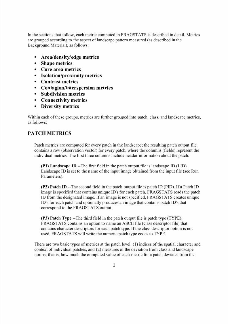
In the sections that follow, each metric computed in FRAGSTATS is described in detail. Metrics
are grouped according to the aspect of landscape pattern measured (as described in the
Background Material), as follows:
• Area/density/edge metrics• Shape metrics
• Core area metrics
• Isolation/proximity metrics
• Contrast metrics
• Contagion/interspersion metrics
• Subdivision metrics
• Connectivity metrics
• Diversity metrics
Within each of these groups, metrics are further grouped into patch, class, and landscape metrics,
as follows:
PATCH METRICS
Patch metrics are computed for every patch in the landscape; the resulting patch output file
contains a row (observation vector) for every patch, where the columns (fields) represent the
individual metrics. The first three columns include header information about the patch:
(P1) Landscape ID.--The first field in the patch output file is landscape ID (LID).
Landscape ID is set to the name of the input image obtained from the input file (see RunParameters).
(P2) Patch ID.--The second field in the patch output file is patch ID (PID). If a Patch ID
image is specified that contains unique ID's for each patch, FRAGSTATS reads the patch
ID from the designated image. If an image is not specified, FRAGSTATS creates unique
ID's for each patch and optionally produces an image that contains patch ID's that
correspond to the FRAGSTATS output.
(P3) Patch Type.--The third field in the patch output file is patch type (TYPE).
FRAGSTATS contains an option to name an ASCII file (class descriptor file) that
contains character descriptors for each patch type. If the class descriptor option is notused, FRAGSTATS will write the numeric patch type codes to TYPE.
There are two basic types of metrics at the patch level: (1) indices of the spatial character and
context of individual patches, and (2) measures of the deviation from class and landscape
norms; that is, how much the computed value of each metric for a patch deviates from the
7/14/2019 Bothanical_Metrics
http://slidepdf.com/reader/full/bothanicalmetrics 3/99
3
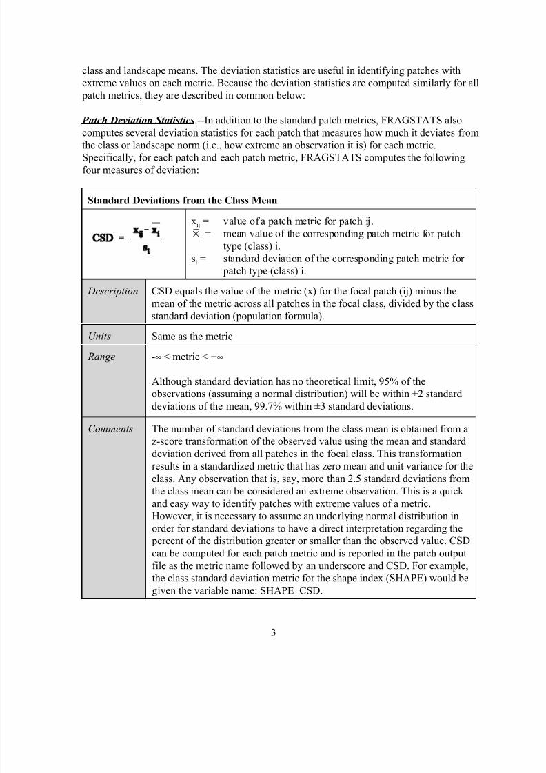
class and landscape means. The deviation statistics are useful in identifying patches with
extreme values on each metric. Because the deviation statistics are computed similarly for all
patch metrics, they are described in common below:
Patch Deviation Statistics.--In addition to the standard patch metrics, FRAGSTATS also
computes several deviation statistics for each patch that measures how much it deviates fromthe class or landscape norm (i.e., how extreme an observation it is) for each metric.
Specifically, for each patch and each patch metric, FRAGSTATS computes the following
four measures of deviation:
Standard Deviations from the Class Mean
xij = value of a patch metric for patch ij.
0i = mean value of the corresponding patch metric for patch
type (class) i.
si = standard deviation of the corresponding patch metric for
patch type (class) i.
Description CSD equals the value of the metric (x) for the focal patch (ij) minus the
mean of the metric across all patches in the focal class, divided by the class
standard deviation (population formula).
Units Same as the metric
Range -4 < metric < +4
Although standard deviation has no theoretical limit, 95% of the
observations (assuming a normal distribution) will be within ±2 standard
deviations of the mean, 99.7% within ±3 standard deviations.
Comments The number of standard deviations from the class mean is obtained from a
z-score transformation of the observed value using the mean and standard
deviation derived from all patches in the focal class. This transformation
results in a standardized metric that has zero mean and unit variance for the
class. Any observation that is, say, more than 2.5 standard deviations from
the class mean can be considered an extreme observation. This is a quick
and easy way to identify patches with extreme values of a metric.
However, it is necessary to assume an underlying normal distribution in
order for standard deviations to have a direct interpretation regarding the
percent of the distribution greater or smaller than the observed value. CSDcan be computed for each patch metric and is reported in the patch output
file as the metric name followed by an underscore and CSD. For example,
the class standard deviation metric for the shape index (SHAPE) would be
given the variable name: SHAPE_CSD.
7/14/2019 Bothanical_Metrics
http://slidepdf.com/reader/full/bothanicalmetrics 4/99
4
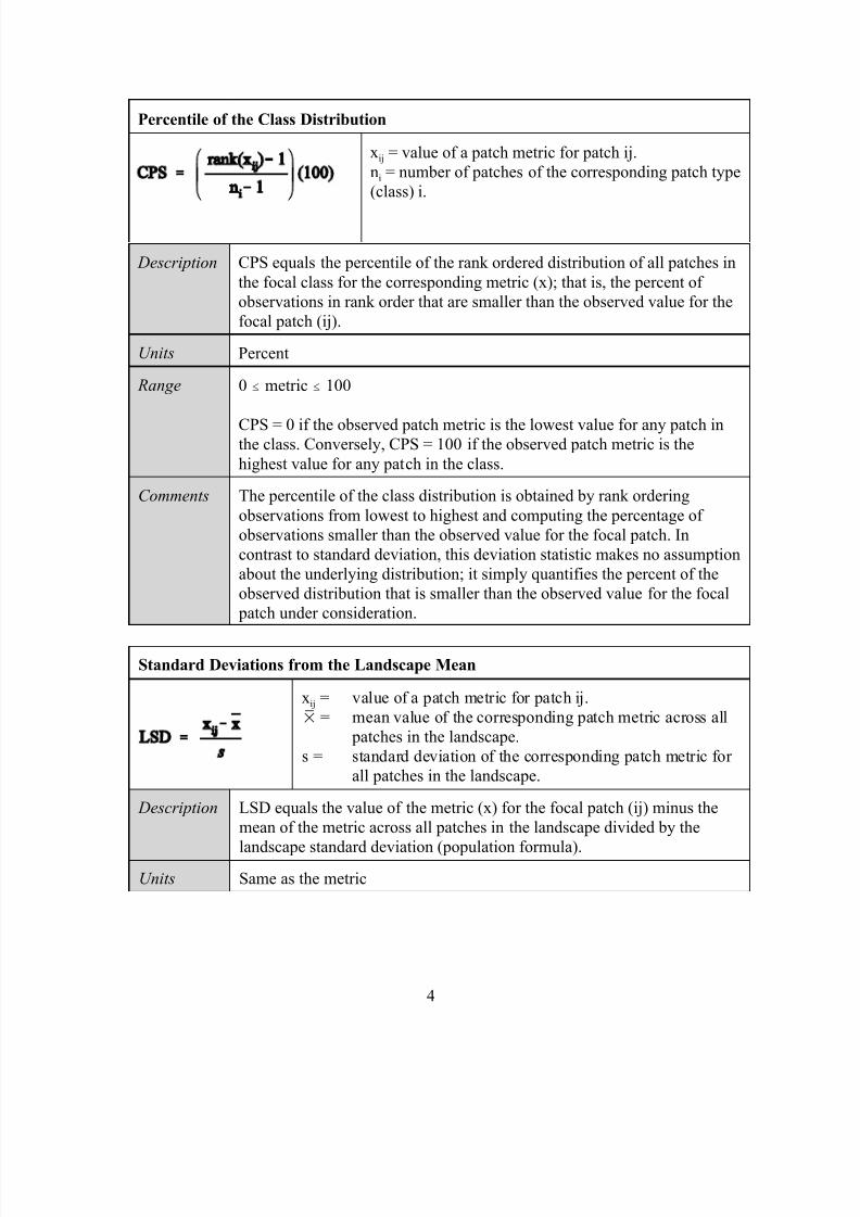
Percentile of the Class Distribution
xij = value of a patch metric for patch ij.
ni = number of patches of the corresponding patch type
(class) i.
Description CPS equals the percentile of the rank ordered distribution of all patches in
the focal class for the corresponding metric (x); that is, the percent of
observations in rank order that are smaller than the observed value for the
focal patch (ij).
Units Percent
Range 0 # metric # 100
CPS = 0 if the observed patch metric is the lowest value for any patch inthe class. Conversely, CPS = 100 if the observed patch metric is the
highest value for any patch in the class.
Comments The percentile of the class distribution is obtained by rank ordering
observations from lowest to highest and computing the percentage of
observations smaller than the observed value for the focal patch. In
contrast to standard deviation, this deviation statistic makes no assumption
about the underlying distribution; it simply quantifies the percent of the
observed distribution that is smaller than the observed value for the focal
patch under consideration.
Standard Deviations from the Landscape Mean
xij = value of a patch metric for patch ij.
0 = mean value of the corresponding patch metric across all
patches in the landscape.
s = standard deviation of the corresponding patch metric for
all patches in the landscape.
Description LSD equals the value of the metric (x) for the focal patch (ij) minus the
mean of the metric across all patches in the landscape divided by the
landscape standard deviation (population formula).Units Same as the metric
7/14/2019 Bothanical_Metrics
http://slidepdf.com/reader/full/bothanicalmetrics 5/99
5
Range -4 < metric < +4
Although standard deviation has no theoretical limit, 95% of the
observations (assuming a normal distribution) will be within ±2 standard
deviations of the mean, 99.7% within ±3 standard deviations.
Comments The number of standard deviations from the landscape mean is obtained
from a z-score transformation of the observed value using the mean and
standard deviation derived from all patches in the landscape. This
transformation results in a standardized metric that has zero mean and unit
variance for the entire landscape. Any observation that is, say, more than
2.5 standard deviations from the landscape mean can be considered an
extreme observation. This is a quick and easy way to identify patches with
extreme values of a metric. However, it is necessary to assume an
underlying normal distribution in order for standard deviations to have a
direct interpretation regarding the percent of the distribution greater or
smaller than the observed value. LSD can be computed for each patchmetric and is reported in the patch output file as the metric name followed
by an underscore and LSD. For example, the landscape standard deviation
metric for the shape index (SHAPE) would be given the variable name:
SHAPE_LSD.
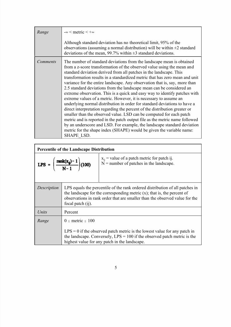
Percentile of the Landscape Distribution
xij = value of a patch metric for patch ij.
N = number of patches in the landscape.
Description LPS equals the percentile of the rank ordered distribution of all patches in
the landscape for the corresponding metric (x); that is, the percent of
observations in rank order that are smaller than the observed value for the
focal patch (ij).
Units Percent
Range 0 # metric # 100
LPS = 0 if the observed patch metric is the lowest value for any patch in
the landscape. Conversely, LPS = 100 if the observed patch metric is the
highest value for any patch in the landscape.
7/14/2019 Bothanical_Metrics
http://slidepdf.com/reader/full/bothanicalmetrics 6/99
6
Comments The percentile of the landscape distribution is obtained by rank ordering
observations from lowest to highest and computing the percentage of
observations smaller than the observed value for the focal patch. In
contrast to standard deviation, this deviation statistic makes no assumption
about the underlying distribution; it simply quantifies the percent of the
observed distribution that is smaller than the observed value for the focal patch under consideration.
CLASS METRICS
Class metrics are computed for every patch type or class in the landscape; the resulting class
output file contains a row (observation vector) for every class, where the columns (fields)
represent the individual metrics. The first two columns include header information about the
class:
(C1) Landscape ID.--The first field in the class output file is landscape ID (LID).
Landscape ID is set to the name of the input image obtained from the input file (see Run
Parameters).
(C2) Patch Type.--The second field in the class output file is patch type (TYPE).
FRAGSTATS contains an option to name an ASCII file (class descriptor file) that
contains character descriptors for each patch type. If the class descriptor option is not
used, FRAGSTATS will write the numeric patch type codes to TYPE.
There are two basic types of metrics at the class level: (1) indices of the amount and spatial
configuration of the class, and (2) distribution statistics that provide first- and second-order statistical summaries of the patch metrics for the focal class. The latter are used to summarize
the mean, area-weighted mean, median, range, standard deviation, and coefficient of
variation in the patch attributes across all patches in the focal class. Because the distribution
statistics are computed similarly for all class metrics, they are described in common below:
Class Distribution Statistics.--Class metrics measure the aggregate properties of the patches
belonging to a single class or patch type. Some class metrics go about this by characterizing
the aggregate properties without distinction among the separate patches that comprise the
class. These metrics are defined elsewhere. Another way to quantify the configuration of
patches at the class level is to summarize the aggregate distribution of the patch metrics for
all patches of the corresponding patch type. In other words, since the class represents anaggregation of patches of the same type, we can characterize the class by summarizing the
patch metrics for the patches that comprise each class. There are many possible first- and
second-order statistics that can be used to summarize the patch distribution. FRAGSTATS
computes the following: (1) mean (MN), (2) area-weighted mean (AMN), (3) median (MD),
(4) range (RA), (5) standard deviation (SD), and (6) coefficient of variation (CV).

7/14/2019 Bothanical_Metrics
http://slidepdf.com/reader/full/bothanicalmetrics 7/99
7
FRAGSTATS computes these distribution statistics for all patch metrics at the class level. In
the class output file, these metrics are labeled by concatenating the metric acronym with an
underscore and the distribution statistic acronym. For example, patch area (AREA) is
summarized at the class level by each of the distribution statistics and reported in the class
output file as follows: mean patch area (AREA_MN), area-weighted mean patch area
(AREA_AMN), median patch area (AREA_MD), range in patch area (AREA_RA), standarddeviation in patch area (AREA_SD), and coefficient of variation in patch area (AREA_CV).
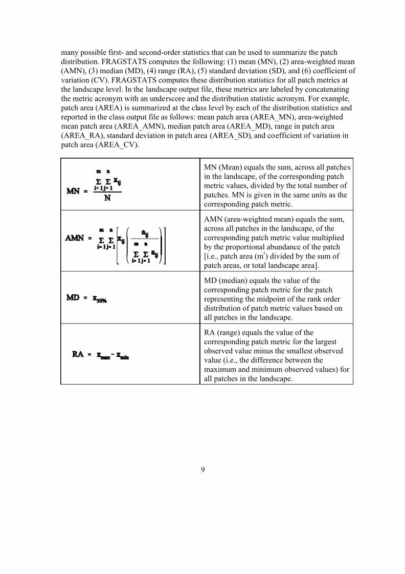
MN (Mean) equals the sum, across all patches
of the corresponding patch type, of the
corresponding patch metric values, divided by
the number of patches of the same type. MN
is given in the same units as the
corresponding patch metric.
AMN (area-weighted mean) equals the sum,
across all patches of the corresponding patch
type, of the corresponding patch metric value
multiplied by the proportional abundance of
the patch [i.e., patch area (m2) divided by the
sum of patch areas].
MD (median) equals the value of the
corresponding patch metric for the patch
representing the midpoint of the rank order
distribution of patch metric values for patches
of the corresponding patch type.
RA (range) equals the value of the
corresponding patch metric for the largest
observed value minus the smallest observed
value (i.e., the difference between the
maximum and minimum observed values) for
patches of the corresponding patch type.
7/14/2019 Bothanical_Metrics
http://slidepdf.com/reader/full/bothanicalmetrics 8/99
8
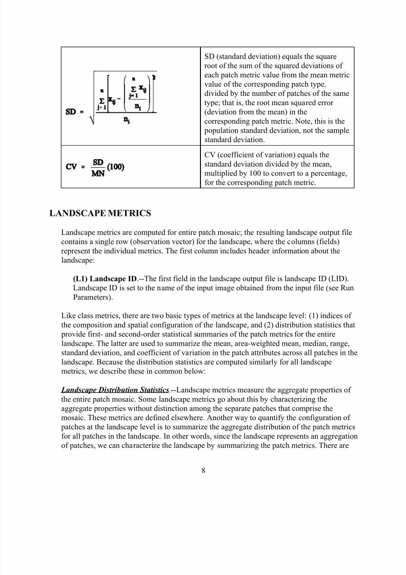
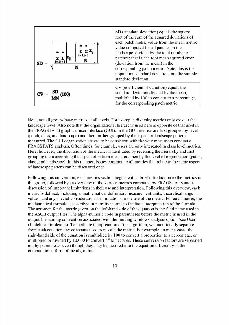
SD (standard deviation) equals the square
root of the sum of the squared deviations of
each patch metric value from the mean metric
value of the corresponding patch type,
divided by the number of patches of the same
type; that is, the root mean squared error (deviation from the mean) in the
corresponding patch metric. Note, this is the
population standard deviation, not the sample
standard deviation.
CV (coefficient of variation) equals the
standard deviation divided by the mean,
multiplied by 100 to convert to a percentage,
for the corresponding patch metric.
LANDSCAPE METRICS
Landscape metrics are computed for entire patch mosaic; the resulting landscape output file
contains a single row (observation vector) for the landscape, where the columns (fields)
represent the individual metrics. The first column includes header information about the
landscape:
(L1) Landscape ID.--The first field in the landscape output file is landscape ID (LID).
Landscape ID is set to the name of the input image obtained from the input file (see Run
Parameters).
Like class metrics, there are two basic types of metrics at the landscape level: (1) indices of
the composition and spatial configuration of the landscape, and (2) distribution statistics that
provide first- and second-order statistical summaries of the patch metrics for the entire
landscape. The latter are used to summarize the mean, area-weighted mean, median, range,
standard deviation, and coefficient of variation in the patch attributes across all patches in the
landscape. Because the distribution statistics are computed similarly for all landscape
metrics, we describe these in common below:
Landscape Distribution Statistics.--Landscape metrics measure the aggregate properties of
the entire patch mosaic. Some landscape metrics go about this by characterizing theaggregate properties without distinction among the separate patches that comprise the
mosaic. These metrics are defined elsewhere. Another way to quantify the configuration of
patches at the landscape level is to summarize the aggregate distribution of the patch metrics
for all patches in the landscape. In other words, since the landscape represents an aggregation
of patches, we can characterize the landscape by summarizing the patch metrics. There are
7/14/2019 Bothanical_Metrics
http://slidepdf.com/reader/full/bothanicalmetrics 9/99
9
many possible first- and second-order statistics that can be used to summarize the patch
distribution. FRAGSTATS computes the following: (1) mean (MN), (2) area-weighted mean
(AMN), (3) median (MD), (4) range (RA), (5) standard deviation (SD), and (6) coefficient of
variation (CV). FRAGSTATS computes these distribution statistics for all patch metrics at
the landscape level. In the landscape output file, these metrics are labeled by concatenating
the metric acronym with an underscore and the distribution statistic acronym. For example, patch area (AREA) is summarized at the class level by each of the distribution statistics and
reported in the class output file as follows: mean patch area (AREA_MN), area-weighted
mean patch area (AREA_AMN), median patch area (AREA_MD), range in patch area
(AREA_RA), standard deviation in patch area (AREA_SD), and coefficient of variation in
patch area (AREA_CV).
MN (Mean) equals the sum, across all patches
in the landscape, of the corresponding patch
metric values, divided by the total number of
patches. MN is given in the same units as the
corresponding patch metric.
AMN (area-weighted mean) equals the sum,
across all patches in the landscape, of the
corresponding patch metric value multiplied
by the proportional abundance of the patch
[i.e., patch area (m2) divided by the sum of
patch areas, or total landscape area].
MD (median) equals the value of the
corresponding patch metric for the patch
representing the midpoint of the rank order distribution of patch metric values based on
all patches in the landscape.
RA (range) equals the value of the
corresponding patch metric for the largest
observed value minus the smallest observed
value (i.e., the difference between the
maximum and minimum observed values) for
all patches in the landscape.
7/14/2019 Bothanical_Metrics
http://slidepdf.com/reader/full/bothanicalmetrics 10/99
10
SD (standard deviation) equals the square
root of the sum of the squared deviations of
each patch metric value from the mean metric
value computed for all patches in the
landscape, divided by the total number of
patches; that is, the root mean squared error (deviation from the mean) in the
corresponding patch metric. Note, this is the
population standard deviation, not the sample
standard deviation.
CV (coefficient of variation) equals the
standard deviation divided by the mean,
multiplied by 100 to convert to a percentage,
for the corresponding patch metric.
Note, not all groups have metrics at all levels. For example, diversity metrics only exist at the
landscape level. Also note that the organizational hierarchy used here is opposite of that used in
the FRAGSTATS graphical user interface (GUI). In the GUI, metrics are first grouped by level
(patch, class, and landscape) and then further grouped by the aspect of landscape pattern
measured. The GUI organization strives to be consistent with the way most users conduct a
FRAGSTATS analysis. Often times, for example, users are only interested in class level metrics.
Here, however, the discussion of the metrics is facilitated by reversing the hierarchy and first
grouping them according the aspect of pattern measured, then by the level of organization (patch,
class, and landscape). In this manner, issues common to all metrics that relate to the same aspect
of landscape pattern can be discussed once.
Following this convention, each metrics section begins with a brief introduction to the metrics in
the group, followed by an overview of the various metrics computed by FRAGSTATS and a
discussion of important limitations in their use and interpretation. Following this overview, each
metric is defined, including a mathematical definition, measurement units, theoretical range in
values, and any special considerations or limitations in the use of the metric. For each metric, the
mathematical formula is described in narrative terms to facilitate interpretation of the formula.
The acronym for the metric given on the left-hand side of the equation is the field name used in
the ASCII output files. The alpha-numeric code in parentheses before the metric is used in the
output file naming convention associated with the moving windows analysis option (see User
Guidelines for details). To facilitate interpretation of the algorithm, we intentionally separate
from each equation any constants used to rescale the metric. For example, in many cases the
right-hand side of the equation is multiplied by 100 to convert a proportion to a percentage, or
multiplied or divided by 10,000 to convert m2 to hectares. These conversion factors are separated
out by parentheses even though they may be factored into the equation differently in the
computational form of the algorithm.
7/14/2019 Bothanical_Metrics
http://slidepdf.com/reader/full/bothanicalmetrics 11/99
11
AREA/DENSITY/EDGE METRICS
The area of each patch comprising a landscape mosaic is perhaps the single most important and
useful piece of information contained in the landscape. Not only is this information the basis for
many of the patch, class, and landscape indices, but patch area has a great deal of ecological
utility in its own right. For example, there is considerable evidence that bird species richness andthe occurrence and abundance of some species are strongly correlated with patch size (e.g.,
Robbins et al. 1989). Most species have minimum area requirements: the minimum area needed
to meet all life history requirements. Some of these species require that their minimum area
requirements be fulfilled in contiguous habitat patches; in other words, the individual habitat
patch must be larger than the species minimum area requirement for them to occupy the patch.
These species are sometimes referred to as “area-sensitive” species. Thus, patch size information
alone could be used to model species richness, patch occupancy, and species distribution patterns
in a landscape given the appropriate empirical relationships derived from field studies.
Similarly, the size and number of patches comprising a class or the entire landscape mosaic is
perhaps the most basic aspect of landscape pattern that can affect myriad processes. For example,although there are myriad effects of habitat fragmentation on individual behavior, habitat use
patterns, and intra- and inter-specific interactions, many of these effects are caused by: (1) a
reduction in habitat area (area effects), and (2) an increase in the proportion of edge-influenced
habitat (edge effects). Briefly, as habitat is lost from the landscape (without being fragmented), at
some point there will be insufficient area of habitat to support even a single individual and the
species will be extirpated from the landscape. This area relationship is expected to vary among
species depending on their minimum area requirements. Moreover, the area threshold for
occupancy may occur when total habitat area is still much greater than the individual’s minimum
area requirement. For example, an individual may not occupy available habitat unless there are
other individuals of the same species occupying the same or nearby patches of habitat, or an
individual’s occupancy may be influenced by what other species are occupying the patch.Similarly, as habitat is lost and simultaneously fragmented into smaller and more isolated
patches, at some point there will be insufficient area of suitable habitat within a home range size
area to support an individual. In either case, the effect of habitat area on the occurrence and
abundance of a species (or species) is referred to as the “area effect.” This is the ultimate
consequence of habitat loss and fragmentation–insufficient habitat quality to support individuals.
Total amount of edge in a landscape is important to many ecological phenomena. In particular, a
great deal of attention has been given to wildlife-edge relationships (Thomas et al. 1978 and
1979, Strelke and Dickson 1980, Morgan and Gates 1982, Logan et al. 1985). In landscape
ecological investigations, much of the presumed importance of spatial pattern is related to edge
effects. The forest edge effect, for example, results primarily from differences in wind and lightintensity and quality reaching a forest patch that alter microclimate and disturbance rates (e.g.,
Gratkowski 1956, Ranney et al. 1981, Chen and Franklin 1990). These changes, in combination
with changes in seed dispersal and herbivory, can influence vegetation composition and structure
(Ranney et al. 1981). The proportion of a forest patch that is affected in this manner is dependent,
therefore, upon patch shape and orientation, and by adjacent land cover. A large but convoluted
7/14/2019 Bothanical_Metrics
http://slidepdf.com/reader/full/bothanicalmetrics 12/99
12
patch, for example, could be entirely edge habitat. It is now widely accepted that edge effects
must be viewed from an organism-centered perspective because edge effects influence organisms
differently; some species have an affinity for edges, some are unaffected, and others are
adversely affected.
One of the most dramatic and well-studied consequences of habitat fragmentation is an increasein the proportional abundance of edge-influenced habitat. Early wildlife management efforts
were focused on maximizing edge habitat because it was believed that most species favored
habitat conditions created by edges and that the juxtaposition of different habitats would increase
species diversity (Leopold 1933). Indeed this concept of edge as a positive influence guided land
management practices for most of the twentieth century. Recent studies, however, have
suggested that changes in microclimate, vegetation, invertebrate populations, predation, brood
parasitism, and competition along forest edges (i.e., edge effects) has resulted in the population
declines of several vertebrate species dependent upon forest interior conditions (e.g., Strelke and
Dickson 1980, Kroodsma 1982, Brittingham and Temple 1983, Wilcove 1985, Temple 1986,
Noss 1988, Yahner and Scott 1988, Robbins et al. 1989). In fact, many of the adverse effects of
forest fragmentation on organisms seem to be directly or indirectly related to these so-called edgeeffects. Forest interior species, therefore, may be sensitive to patch shape because for a given
patch size, the more complex the shape, the larger the edge-to-interior ratio. Total class edge in a
landscape, therefore, often is the most critical piece of information in the study of fragmentation,
and many of the class indices directly or indirectly reflect the amount of class edge. Similarly,
the total amount of edge in a landscape is directly related to the degree of spatial heterogeneity in
that landscape.
FRAGSTATS Metrics.--FRAGSTATS computes several simple statistics representing area and
perimeter (or edge) at the patch, class, and landscape levels. Area metrics quantify landscape
composition, not landscape configuration. As noted above, the area (AREA) of each patch
comprising a landscape mosaic is perhaps the single most important and useful piece of information contained in the landscape. However, the size of a patch may not be as important as
the extensiveness of the patch for some organisms and processes. Radius of gyration (GYRATE)
is a measure of patch extent; that is, how far across the landscape a patch extends its reach. All
other things equal, the larger the patch, the larger the radius of gyration. Similarly, holding area
constant, the more extensive the patch (i.e., elongated and less compact), the greater the radius of
gyration. The radius of gyration can be considered a measure of the average distance an organism
can move within a patch before encountering the patch boundary from a random starting point.
When aggregated at the class or landscape level, radius of gyration provides a measure of
landscape connectivity (known as correlation length) that represents the average traversability of
the landscape for an organism that is confined to remain within a single patch.
Class area (CA) and percentage of landscape (PLAND) are measures of landscape composition;
specifically, how much of the landscape is comprised of a particular patch type. This is an
important characteristic in a number of ecological applications. For example, an important by-
product of habitat fragmentation is habitat loss. In the study of forest fragmentation, therefore, it
is important to know how much of the target patch type (habitat) exists within the landscape. In
7/14/2019 Bothanical_Metrics
http://slidepdf.com/reader/full/bothanicalmetrics 13/99
13
addition, although many vertebrate species that specialize on a particular habitat have minimum
area requirements (e.g., Robbins et al. 1989), not all species require that suitable habitat to be
present in a single contiguous patch. For example, northern spotted owls have minimum area
requirements for late-seral forest that varies geographically; yet, individual spotted owls use late-
seral forest that may be distributed among many patches (Forsman et al. 1984). For this species,
late-seral forest area might be a good index of habitat suitability within landscapes the size of spotted owl home ranges (Lehmkuhl and Raphael 1993). In addition to its direct interpretive
value, class area (in absolute or relative terms) is used in the computations for many of the class
and landscape metrics.
FRAGSTATS computes several simple statistics representing the number or density of patches,
the average size or radius of gyration of patches, and the variation in patch size or radius of
gyration at the class and landscape levels. These metrics usually are best considered as
representing landscape configuration, even though they are not spatially explicit measures.
Number of patches (NP) or patch density (PD) of a particular habitat type may affect a variety of
ecological processes, depending on the landscape context. For example, the number or density of
patches may determine the number of subpopulations in a spatially-dispersed population, or metapopulation, for species exclusively associated with that habitat type. The number of
subpopulations could influence the dynamics and persistence of the metapopulation (Gilpin and
Hanski 1991). The number or density of patches also can alter the stability of species interactions
and opportunities for coexistence in both predator-prey and competitive systems (Kareiva 1990).
The number or density of patches in a landscape mosaic (pooled across patch types) can have the
same ecological applicability, but more often serves as a index of spatial heterogeneity of the
entire landscape mosaic. A landscape with a greater number or density of patches has a finer
grain; that is, the spatial heterogeneity occurs at a finer resolution. Although the number or
density of patches in a class or in the landscape may be fundamentally important to a number of
ecological processes, often it does not have any interpretive value by itself because it conveys no
information about the area or distribution of patches. Number or density of patches is probablymost valuable, however, as the basis for computing other, more interpretable, metrics.
In addition to these primary metrics, FRAGSTATS also summarizes the distribution of patch
area and extent (radius of gyration) across all patches at the class and landscape levels. For
example, the distribution of patch area (AREA) is summarized by its mean and variability. These
summary measures provide a way to characterize the distribution of area among patches at the
class or landscape level. For example, progressive reduction in the size of habitat fragments is a
key component of habitat fragmentation. Thus, a landscape with a smaller mean patch size for
the target patch type than another landscape might be considered more fragmented. Similarly,
within a single landscape, a patch type with a smaller mean patch size than another patch type
might be considered more fragmented. Thus, mean patch size can serve as a habitatfragmentation index, although the limitations discussed below may reduce its utility in this
respect.
Mean patch size at the class level is a function of the number of patches in the class and total
class area. In contrast, patch density is a function of total landscape area. Therefore, at the class
7/14/2019 Bothanical_Metrics
http://slidepdf.com/reader/full/bothanicalmetrics 14/99
14
level, these two indices represent slightly different aspects of class structure. For example, two
landscapes could have the same number and size distribution of patches for a given class and
thus have the same mean patch size; yet, if total landscape area differed, patch density could be
very different between landscapes. Alternatively, two landscapes could have the same number of
patches and total landscape area and thus have the same patch density; yet, if class area differed,
mean patch size could be very different between landscapes. These differences should be kept inmind when selecting class metrics for a particular application. In addition, although mean patch
size is derived from the number of patches, it does not convey any information about how many
patches are present. A mean patch size of 10 ha could represent 1 or 100 patches and the
difference could have profound ecological implications. Furthermore, mean patch size represents
the average condition. Variation in patch size may convey more useful information. For example,
a mean patch size of 10 ha could represent a class with 5 10-ha patches or a class with 2-, 3-, 5-,
10-, and 30-ha patches, and this difference could be important ecologically. For these reasons,
mean patch size is probably best interpreted in conjunction with total class area, patch density (or
number of patches), and patch size variability. At the landscape level, mean patch size and patch
density are both a function of number of patches and total landscape area. In contrast to the class
level, these indices are completely redundant. Although both indices may be useful for "describing" 1 or more landscapes, they would never be used simultaneously in a statistical
analysis of landscape structure.
In many ecological applications, second-order statistics, such as the variation in patch size, may
convey more useful information than first-order statistics, such as mean patch size. Variability in
patch size measures a key aspect of landscape heterogeneity that is not captured by mean patch
size and other first-order statistics. For example, consider 2 landscapes with the same patch
density and mean patch size, but with very different levels of variation in patch size. Greater
variability indicates less uniformity in pattern either at the class level or landscape level and may
reflect differences in underlying processes affecting the landscapes. Variability is a difficult thing
to summarize in a single metric. FRAGSTATS computes three of the simplest measures of variability–range, standard deviation, and coefficient of variation.
Patch size standard deviation (AREA_SD) is a measure of absolute variation; it is a function of
the mean patch size and the difference in patch size among patches. Thus, although patch size
standard deviation conveys information about patch size variability, it is a difficult parameter to
interpret without doing so in conjunction with mean patch size because the absolute variation is
dependent on mean patch size. For example, two landscapes may have the same patch size
standard deviation, e.g., 10 ha; yet one landscape may have a mean patch size of 10 ha, while the
other may have a mean patch size of 100 ha. In this case, the interpretations of landscape pattern
would be very different, even though absolute variation is the same. Specifically, the former
landscape has greatly varying and smaller patch sizes, while the latter has more uniformly-sizedand larger patches. For this reason, patch size coefficient of variation (AREA_CV) is generally
preferable to standard deviation for comparing variability among landscapes. Patch size
coefficient of variation measures relative variability about the mean (i.e., variability as a
percentage of the mean), not absolute variability. Thus, it is not necessary to know mean patch
size to interpret the coefficient of variation. Nevertheless, patch size coefficient of variation also
7/14/2019 Bothanical_Metrics
http://slidepdf.com/reader/full/bothanicalmetrics 15/99
15
can be misleading with regards to landscape structure in the absence of information on the
number of patches or patch density and other structural characteristics. For example, two
landscapes may have the same patch size coefficient of variation, e.g., 100%; yet one landscape
may have 100 patches with a mean patch size of 10 ha, while the other may have 10 patches with
a mean patch size of 100 ha. In this case, the interpretations of landscape structure could be very
different, even though the coefficient of variation is the same. Ultimately, the choice of standarddeviation or coefficient of variation will depend on whether absolute or relative variation is more
meaningful in a particular application. Because these measures are not wholly redundant, it may
be meaningful to interpret both measures in some applications.
It is important to keep in mind that both standard deviation and coefficient of variation assume a
normal distribution about the mean. In a real landscape, the distribution of patch sizes may be
highly irregular. It may be more informative to inspect the actual distribution itself, rather than
relying on summary statistics such as these that make assumptions about the distribution and
therefore can be misleading. Also, note that patch size standard deviation and coefficient of
variation can equal 0 under 2 different conditions: (1) when there is only 1 patch in the
landscape; and (2) when there is more than 1 patch, but they are all the same size. In both cases,there is no variability in patch size, yet the ecological interpretations could be different.
FRAGSTATS computes several statistics representing the amount of perimeter (or edge) at the
patch, class, and landscape levels. Edge metrics usually are best considered as representing
landscape configuration, even though they are not spatially explicit at all. At the patch level, edge
is a function of patch perimeter (PERIM). At the class and landscape levels, edge can be
quantified in other ways. Total edge (TE) is an absolute measure of total edge length of a
particular patch type (class level) or of all patch types (landscape level). In applications that
involve comparing landscapes of varying size, this index may not be useful. Edge density (ED)
standardizes edge to a per unit area basis that facilitates comparisons among landscapes of
varying size. However, when comparing landscapes of identical size, total edge and edge densityare completely redundant. Alternatively, the amount of edge present in a landscape can be
compared to that expected for a landscape of the same size but with a simple geometric shape
(square) and no internal edge. Landscape shape index (LSI) does this. This index measures the
perimeter-to-area ratio for the landscape as a whole. This index is identical to the habitat
diversity index proposed by Patton (1975), except that we apply the index at the class level as
well. Landscape shape index is identical to the shape index at the patch level (SHAPE), except
that it treats the entire landscape as if it were one patch and any patch edges (or class edges) as
though they belong to the perimeter. The landscape boundary must be included as edge in the
calculation in order to use a square standard for comparison. Unfortunately, this may not be
meaningful in cases where the landscape boundary does not represent true edge and/or the actual
shape of the landscape is of no particular interest. In this case, the total amount of true edge, or some other index based on edge, would probably be more meaningful. If the landscape boundary
represents true edge or the shape of the landscape is particularly important, then the landscape
shape index can be a useful index, especially when comparing among landscapes of varying
sizes.
7/14/2019 Bothanical_Metrics
http://slidepdf.com/reader/full/bothanicalmetrics 16/99
16
Limitations.--Area metrics have limitations imposed by the scale of investigation. Minimum
patch size and landscape extent set the lower and upper limits of these area metrics, respectively.
These are critical limits to recognize because they establish the lower and upper limits of
resolution for the analysis of landscape composition and pattern. Otherwise, area metrics have
few limitations. All edge indices are affected by the resolution of the image. Generally, the finer
the resolution (i.e., the greater the detail with which edges are delineated), the greater the edgelength. At coarse resolutions, edges may appear as relatively straight lines; whereas, at finer
resolutions, edges may appear as highly convoluted lines. Thus, values calculated for edge
metrics should not be compared among images with different resolutions. In addition, patch
perimeter and the length of edges will be biased upward in raster images because of the stair-step
patch outline, and this will affect all edge indices. The magnitude of this bias will vary in relation
to the grain or resolution of the image, and the consequences of this bias with regards to the use
and interpretation of these indices must be weighed relative to the phenomenon under
investigation.
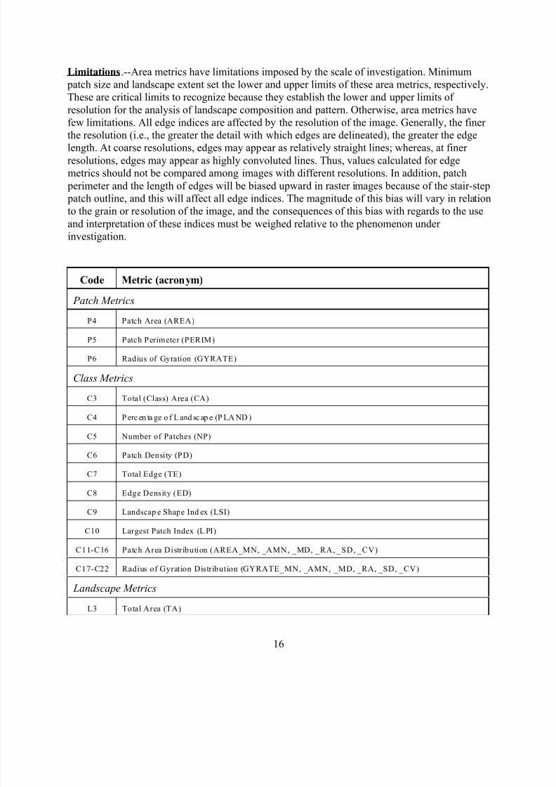
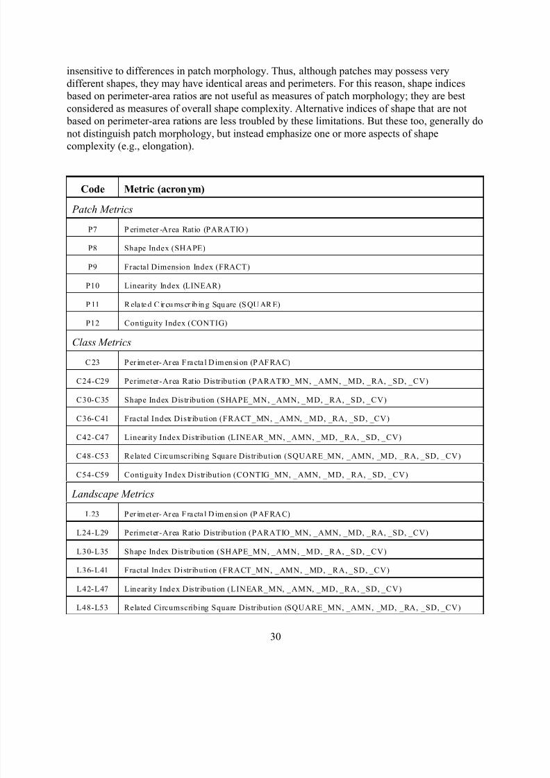
Code Metric (acronym)
Patch Metrics
P4 Patch Area (AREA)
P5 Patch Perimeter (PERIM)
P6 Radius of Gyration (GYRATE)
Class Metrics
C3 Total (Class) Area (CA)
C4 P erc en ta ge o f L and sc ap e (P LA ND )
C5 Number of Patches (NP)
C6 Patch Density (PD)
C7 Total Edge (TE)
C8 Edge Density (ED)
C9 Landscap e Shape Ind ex (LSI)
C10 Largest Patch Index (L PI)
C11-C16 Patch Area Distribution (AREA_MN, _AMN, _MD, _RA, _SD, _CV)
C17-C22 Radius of Gyration Distribution (GYRATE_MN, _AMN, _MD, _RA, _SD, _CV)
Landscape Metrics
L3 Total Area (TA)
7/14/2019 Bothanical_Metrics
http://slidepdf.com/reader/full/bothanicalmetrics 17/99
17
L5 Number of Patches (NP)
L6 Patch Density (PD)
L7 Total Edge (TE)
L8 Edge Density (ED)
L9 Landscap e Shape Ind ex (LSI)
L10 Largest Patch Index (L PI)
L11-L16 Patch Area Distribution (AREA_MN, _AMN, _MD, _RA, _SD, _CV)
L17-L22 Radius of Gyration Distribution (GYRATE_MN, _AMN, _MD, _RA, _SD, _CV)
(P4) Area
aij = area (m2
) of patch ij.
Description AREA equals the area (m2) of the patch, divided by 10,000 (to convert to
hectares).
Units Hectares
Range AREA > 0, without limit.
The range in AREA is limited by the grain and extent of the image, and in a
particular application, AREA may be further limited by the specification of aminimum patch size that is larger than the grain.
Comments The area of each patch comprising a landscape mosaic is perhaps the single
most important and useful piece of information contained in the landscape. Not
only is this information the basis for many of the patch, class, and landscape
indices, but patch area has a great deal of ecological utility in its own right.
Note that the choice of the 4-neighbor or 8-neighbor rule for delineating
patches will have an impact on this metric.
(P5) Perimeter
pij = perimeter (m) of patch ij.
Description PERIM equals the perimeter (m) of the patch, including any internal holes in
the patch.

7/14/2019 Bothanical_Metrics
http://slidepdf.com/reader/full/bothanicalmetrics 18/99
18
Units Meters
Range PERIM > 0, without limit.
Comments Patch perimeter is another fundamental piece of information available about a
landscape and is the basis for many class and landscape metrics. Specifically,
the perimeter of a patch is treated as an edge, and the intensity and distribution
of edges constitutes a major aspect of landscape pattern. In addition, the
relationship between patch perimeter and patch area is the basis for most shape
indices.
(P6) Radius of Gyration
hijr = distance (m) between cell ijr [located within patch ij]
and the centroid of patch ij (the average location),
based on cell center-to-cell center distance.
z = number of cells in patch ij.
Description GYRATE equals the mean distance (m) between each cell in the patch and the
patch centroid.
Units Meters
Range GYRATE $ 0, without limit.
GYRATE = 0 when the patch consists of a single cell and increases without
limit as the patch increases in extent. GYRATE achieves its maximum value
when the patch comprises the entire landscape.
Comments Radius of gyration is a measure of patch extent; thus it is effected by both patch
size and patch compaction. Note that the choice of the 4-neighbor or 8-neighbor
rule for delineating patches will have an impact on this metric.
(C3) Total (Class) Area
aij = area (m2) of patch ij.
Description CA equals the sum of the areas (m2
) of all patches of the corresponding patchtype, divided by 10,000 (to convert to hectares); that is, total class area.
Units Hectares
7/14/2019 Bothanical_Metrics
http://slidepdf.com/reader/full/bothanicalmetrics 19/99
19
Range CA > 0, without limit.
CA approaches 0 as the patch type becomes increasing rare in the landscape.
CA = TA when the entire landscape consists of a single patch type; that is,
when the entire image is comprised of a single patch.
Comments Class area is a measure of landscape composition; specifically, how much of
the landscape is comprised of a particular patch type. In addition to its direct
interpretive value, class area is used in the computations for many of the class
and landscape metrics.
(C4) Percentage of Landscape
Pi = proportion of the landscape occupied by patch
type (class) i.
aij = area (m2) of patch ij.
A = total landscape area (m2).
Description PLAND equals the sum of the areas (m2) of all patches of the corresponding
patch type, divided by total landscape area (m2), multiplied by 100 (to convert
to a percentage); in other words, PLAND equals the percentage the landscape
comprised of the corresponding patch type.
Units Percent
Range 0 < PLAND # 100
PLAND approaches 0 when the corresponding patch type (class) becomesincreasingly rare in the landscape. PLAND = 100 when the entire landscape
consists of a single patch type; that is, when the entire image is comprised of a
single patch.
Comments Percentage of landscape quantifies the proportional abundance of each patch
type in the landscape. Like total class area, it is a measure of landscape
composition important in many ecological applications. However, because
PLAND is a relative measure, it may be a more appropriate measure of
landscape composition than class area for comparing among landscapes of
varying sizes.
(C5) Number of Patches
ni = number of patches in the landscape of patch type (class) i.

7/14/2019 Bothanical_Metrics
http://slidepdf.com/reader/full/bothanicalmetrics 20/99
20
Description NP equals the number of patches of the corresponding patch type (class).
Units None
Range NP $ 1, without limit.
NP = 1 when the landscape contains only 1 patch of the corresponding patch
type; that is, when the class consists of a single patch.
Comments Number of patches of a particular patch type is a simple measure of the extent
of subdivision or fragmentation of the patch type. Although the number of
patches in a class may be fundamentally important to a number of ecological
processes, often it has limited interpretive value by itself because it conveys no
information about area, distribution, or density of patches. Of course, if total
landscape area and class area are held constant, then number of patches conveys
the same information as patch density or mean patch size and may be a useful
index to interpret. Number of patches is probably most valuable, however, as
the basis for computing other, more interpretable, metrics. Note that the choiceof the 4-neighbor or 8-neighbor rule for delineating patches will have an impact
on this metric.
(C6) Patch Density
ni = number of patches in the landscape of patch type
(class) i.
A = total landscape area (m2).
Description PD equals the number of patches of the corresponding patch type (NP) divided
by total landscape area, multiplied by 10,000 and 100 (to convert to 100hectares).
Units Number per 100 hectares
Range PD > 0, constrained by cell size.
PD is ultimately constrained by the grain size of the raster image, because the
maximum PD is attained when every cell is a separate patch. Therefore,
ultimately cell size will determine the maximum number of patches per unit
area. However, the maximum density of patches of a single class is attained
when every other cell is of that focal class (i.e., in a checker board manner; because adjacent cells of the same class would be in the same patch).
7/14/2019 Bothanical_Metrics
http://slidepdf.com/reader/full/bothanicalmetrics 21/99
21
Comments Patch density is a limited, but fundamental, aspect of landscape pattern. Patch
density has the same basic utility as number of patches as an index, except that
it expresses number of patches on a per unit area basis that facilitates
comparisons among landscapes of varying size. Of course, if total landscape
area is held constant, then patch density and number of patches convey the
same information. Like number of patches, patch density often has limitedinterpretive value by itself because it conveys no information about the sizes
and spatial distribution of patches. Note that the choice of the 4-neighbor or 8-
neighbor rule for delineating patches will have an impact on this metric.
(C7) Total Edge
eik = total length (m) of edge in landscape between patch types
(classes) i and k; includes landscape boundary segments
involving patch type i.
Description TE equals the sum of the lengths (m) of all edge segments involving thecorresponding patch type. If a landscape border is present, TE includes
landscape boundary segments involving the corresponding patch type and
representing true edge only (i.e., contrast weight > 0). If a landscape border is
absent, TE includes a user-specified proportion of landscape boundary
segments involving the corresponding patch type. Regardless of whether a
landscape border is present or not, TE includes a user-specified proportion of
background edge segments involving the corresponding patch type.
Units Meters
Range TE$
0, without limit.
TE = 0 when there is no class edge in the landscape; that is, when the entire
landscape and landscape border, if present, consists of the corresponding patch
type and the user specifies that none of the landscape boundary and background
edge be treated as edge.
Comments Total edge at the class level is an absolute measure of total edge length of a
particular patch type. In applications that involve comparing landscapes of
varying size, this index may not be as useful as edge density (see below).
However, when comparing landscapes of identical size, total edge and edge
density are completely redundant.
7/14/2019 Bothanical_Metrics
http://slidepdf.com/reader/full/bothanicalmetrics 22/99
22
(C8) Edge Density
eik = total length (m) of edge in landscape between patch
types (classes) i and k; includes landscape boundary
segments involving patch type i.
A = total landscape area (m2
).
Description ED equals the sum of the lengths (m) of all edge segments involving the
corresponding patch type, divided by the total landscape area (m2), multiplied
by 10,000 (to convert to hectares). If a landscape border is present, ED includes
landscape boundary segments involving the corresponding patch type and
representing true edge only (i.e., contrast weight > 0). If a landscape border is
absent, ED includes a user-specified proportion of landscape boundary
segments involving the corresponding patch type. Regardless of whether a
landscape border is present or not, ED includes a user-specified proportion of
background edge segments involving the corresponding patch type.
Units Meters per hectare
Range ED $ 0, without limit.
ED = 0 when there is no class edge in the landscape; that is, when the entire
landscape and landscape border, if present, consists of the corresponding patch
type and the user specifies that none of the landscape boundary and background
edge be treated as edge.
Comments Edge density at the class level has the same utility and limitations as Total Edge
(see Total Edge description), except that edge density reports edge length on a
per unit area basis that facilitates comparison among landscapes of varying size.
(C9) Landscape Shape Index
e*ik = total length (m) of edge in landscape between patch types
(classes) i and k; includes the entire landscape boundary and
all background edge segments, regardless of whether they
represent edge or not.
A = total landscape area (m2).
Description LSI equals .25 (adjustment for raster format) times the sum of the landscape boundary (regardless of whether it represents true edge or not) and all edge
segments (m) within the landscape boundary involving the corresponding patch
type (including those bordering background), divided by the square root of the
total landscape area (m2).
7/14/2019 Bothanical_Metrics
http://slidepdf.com/reader/full/bothanicalmetrics 23/99
23
Units None
Range LSI $ 1, without limit.
LSI = 1 when the landscape consists of a single square patch of the
corresponding type; LSI increases without limit as landscape shape becomesmore irregular and/or as the length of edge within the landscape of the
corresponding patch type increases.
Comments Landscape shape index provides a standardized measure of total edge or edge
density that adjusts for the size of the landscape. Because it is standardized, it
has a direct interpretation, in contrast to total edge, for example, that is only
meaningful relative to the size of the landscape.
(C10) Largest Patch Index
aij = area (m2
) of patch ij.A = total landscape area (m2).
Description LPI equals the area (m2) of the largest patch of the corresponding patch type
divided by total landscape area, multiplied by 100 (to convert to a percentage);
in other words, LPI equals the percentage of the landscape comprised by the
largest patch.
Units Percent
Range 0 < LPI # 100
LPI approaches 0 when the largest patch of the corresponding patch type is
increasing small. LPI = 100 when the entire landscape consists of a single patch
of the corresponding patch type; that is, when the largest patch comprises 100%
of the landscape.
Comments Largest patch index at the class level quantifies the percentage of total
landscape area comprised by the largest patch. As such, it is a simple measure
of dominance.
(L3) Total Area
A = total landscape area (m2).
7/14/2019 Bothanical_Metrics
http://slidepdf.com/reader/full/bothanicalmetrics 24/99
24
Description TA equals the total area (m2) of the landscape, divided by 10,000 (to convert to
hectares). TA excludes the area of any background patches within the
landscape.
Units Hectares
Range TA > 0, without limit.
Comments Total area (TA) often does not have a great deal of interpretive value with
regards to evaluating landscape pattern, but it is important because it defines
the extent of the landscape. Moreover, total landscape area is used in the
computations for many of the class and landscape metrics. Total landscape area
is included as both a class and landscape index (and included in the
corresponding output files) because it is important regardless of whether the
primary interest is in class or landscape indices.
(L5) Number of Patches
N = total number of patches in the landscape.
Description NP equals the number of patches in the landscape. Note, NP does not include
any background patches within the landscape or patches in the landscape
border.
Units None
Range NP $ 1, without limit.
NP = 1 when the landscape contains only 1 patch.
Comments Number of patches often it has limited interpretive value by itself because it
conveys no information about area, distribution, or density of patches. Of
course, if total landscape area is held constant, then number of patches conveys
the same information as patch density or mean patch size and may be a useful
index to interpret. Number of patches is probably most valuable, however, as
the basis for computing other, more interpretable, metrics. Note that the choice
of the 4-neighbor or 8-neighbor rule for delineating patches will have an impact
on this metric.
(L6) Patch Density
N = total number of patches in the landscape.
A = total landscape area (m2).

7/14/2019 Bothanical_Metrics
http://slidepdf.com/reader/full/bothanicalmetrics 25/99
25
Description PD equals the number of patches in the landscape, divided by total landscape
area, multiplied by 10,000 and 100 (to convert to 100 hectares). Note, PD does
not include any background patches within the landscape or patches in the
landscape border.
Units Number per 100 hectares
Range PD > 0, constrained by cell size.
PD is ultimately constrained by the grain size of the raster image, because the
maximum PD is attained when every cell is a separate patch.
Comments Patch density is a limited, but fundamental, aspect of landscape pattern. Patch
density has the same basic utility as number of patches as an index, except that
it expresses number of patches on a per unit area basis that facilitates
comparisons among landscapes of varying size. Of course, if total landscape
area is held constant, then patch density and number of patches convey the
same information. Like number of patches, patch density often has limitedinterpretive value by itself because it conveys no information about the sizes
and spatial distribution of patches. Note that the choice of the 4-neighbor or 8-
neighbor rule for delineating patches will have an impact on this metric.
(L7) Total Edge
TE = E E = total length (m) of edge in landscape.
Description TE equals the sum of the lengths (m) of all edge segments in the landscape. If a
landscape border is present, TE includes landscape boundary segments
representing true edge only (i.e., contrast weight > 0). If a landscape border isabsent, TE includes a user-specified proportion of the landscape boundary.
Regardless of whether a landscape border is present or not, TE includes a user-
specified proportion of background edge.
Units Meters
Range TE $ 0, without limit.
TE = 0 when there is no edge in the landscape; that is, when the entire
landscape and landscape border, if present, consists of a single patch and the
user specifies that none of the landscape boundary and background edge betreated as edge.
7/14/2019 Bothanical_Metrics
http://slidepdf.com/reader/full/bothanicalmetrics 26/99
26
Comments Total edge is an absolute measure of total edge length of a particular patch type.
In applications that involve comparing landscapes of varying size, this index
may not be as useful as edge density (see below). However, when comparing
landscapes of identical size, total edge and edge density are completely
redundant.
(L8) Edge Density
E = total length (m) of edge in landscape.
A = total landscape area (m2).
Description ED equals the sum of the lengths (m) of all edge segments in the landscape,
divided by the total landscape area (m2), multiplied by 10,000 (to convert to
hectares). If a landscape border is present, ED includes landscape boundary
segments representing true edge only (i.e., contrast weight > 0). If a landscape
border is absent, ED includes a user-specified proportion of the landscape boundary. Regardless of whether a landscape border is present or not, ED
includes a user-specified proportion of background edge.
Units Meters per hectare
Range ED $ 0, without limit.
ED = 0 when there is no edge in the landscape; that is, when the entire
landscape and landscape border, if present, consists of a single patch and the
user specifies that none of the landscape boundary and background edge be
treated as edge.
Comments Edge density has the same utility and limitations as Total Edge (see Total Edge
description), except that edge density reports edge length on a per unit area
basis that facilitates comparison among landscapes of varying size.
(L9) Landscape Shape Index
E* = total length (m) of edge in landscape; includes entire
landscape boundary and background edge segments
regardless of whether they represent edge or not.
A = total landscape area (m2).
Description LSI equals .25 (adjustment for raster format) times the sum of the landscape
boundary (regardless of whether it represents true edge or not) and all edge
segments (m) within the landscape boundary (including those bordering
background), divided by the square root of the total landscape area (m2).
7/14/2019 Bothanical_Metrics
http://slidepdf.com/reader/full/bothanicalmetrics 27/99
27
Units None
Range LSI $ 1, without limit.
LSI = 1 when the landscape consists of a single circular (vector) or square
(raster) patch; LSI increases without limit as landscape shape becomes moreirregular and/or as the length of edge within the landscape increases.
Comments Landscape shape index provides a standardized measure of total edge or edge
density that adjusts for the size of the landscape. Because it is standardized, it
has a direct interpretation, in contrast to total edge, for example, that is only
meaningful relative to the size of the landscape.
(L10) Largest Patch Index
aij = area (m2) of patch ij.
A = total landscape area (m2
).
Description LPI equals the area (m2) of the largest patch in the landscape divided by total
landscape area (m2), multiplied by 100 (to convert to a percentage); in other
words, LPI equals the percent of the landscape that the largest patch comprises.
Units Percent
Range 0 < LPI # 100
LPI approaches 0 when the largest patch in the landscape is increasingly small.LPI = 100 when the entire landscape consists of a single patch; that is, when the
largest patch comprises 100% of the landscape.
Comments Largest patch index quantifies the percentage of total landscape area comprised
by the largest patch. As such, it is a simple measure of dominance.
SHAPE METRICS
Background.--The interaction of patch shape and size can influence a number of important
ecological processes. Patch shape has been shown to influence inter-patch processes such assmall mammal migration (Buechner 1989) and woody plant colonization (Hardt and Forman
1989), and may influence animal foraging strategies (Forman and Godron 1986). However, the
primary significance of shape in determining the nature of patches in a landscape seems to be
related to the "edge effect" (see discussion of edge effects for Area/Density/Edge Metrics).Shape
is a difficult parameter to quantify concisely in a metric.
7/14/2019 Bothanical_Metrics
http://slidepdf.com/reader/full/bothanicalmetrics 28/99
28
FRAGSTATS Metrics.--FRAGSTATS computes several metrics that quantify landscape
configuration in terms of the complexity of patch shape at the patch, class, and landscape levels.
Most of these shape metrics are based on perimeter-area relationships. Perhaps the simplest
shape index is a straightforward perimeter-area ratio (PARATIO). A problem with this metric as
a shape index is that it varies with the size of the patch. For example, holding shape constant, an
increase in patch size will cause a decrease in the perimeter-area ratio. Patton (1975) proposed adiversity index based on shape for quantifying habitat edge for wildlife species and as a means
for comparing alternative habitat improvement efforts (e.g., wildlife clearings). This shape index
(SHAPE) measures the complexity of patch shape compared to a standard shape (square) of the
same size, and therefore alleviates the size dependency problem of PARATIO. This shape index
is widely applicable in landscape ecological research (Forman and Godron 1986).
Another other basic type of shape index based on perimeter-area relationships is the fractal
dimension index. In landscape ecological research, patch shapes are frequently characterized via
the fractal dimension (Krummel et al. 1987, Milne 1988, Turner and Ruscher 1988, Iverson
1989, Ripple et al. 1991). The appeal of fractal analysis is that it can be applied to spatial features
over a wide variety of scales. Mandelbrot (1977, 1982) introduced the concept of fractal, ageometric form that exhibits structure at all spatial scales, and proposed a perimeter-area method
to calculate the fractal dimension of natural planar shapes. The perimeter-area method quantifies
the degree of complexity of the planar shapes. The degree of complexity of a polygon is
characterized by the fractal dimension (D), such that the perimeter (P) of a patch is related to the
area (A) of the same patch by P . /AD (i.e., log P . ½D log A). For simple Euclidean shapes
(e.g., circles and rectangles), P . /A and D = 1 (the dimension of a line). As the polygons
become more complex, the perimeter becomes increasingly plane-filling and P . A with D 6 2.
Although fractal analysis typically has not been used to characterize individual patches in
landscape ecological research, we use this relationship to calculate the fractal dimension of each
patch separately. Note that the value of the fractal dimension calculated in this manner is
dependent upon patch size and/or the units used (Rogers 1993). Therefore, caution should beexercised when using this fractal dimension index as a measure of patch shape complexity.
Fractal analysis usually is applied to the entire landscape mosaic using the perimeter-area
relationship A = k P2/D, where k is a constant (Burrough 1986). If sufficient data are available, the
slope of the line obtained by regressing log(P) on log(A) is equal to 2/D (Burrough 1986). Note,
fractal dimension computed in this manner is equal to 2 divided by the slope; D is not equal to
the slope (Krummel et al. 1987) nor is it equal to 2 times the slope (e.g., O'Neill et al. 1988,
Gustafson and Parker 1992). We refer to this index as the perimeter area fractal dimension
(PAFRAC) in FRAGSTATS. Because this index employs regression analysis, it is subject to
spurious results when sample sizes are small. In landscapes with only a few patches, it is not
unusual to get values that greatly exceed the theoretical limits of this index. Thus, this index is probably only useful if sample sizes are large (e.g., n > 20). If insufficient data are available, an
alternative to the regression approach is to calculate the mean patch fractal dimension
(FRACT_MN) based on the fractal dimension of each patch, or the area-weighted mean patch
fractal dimension (FRACT_AMN) at the class and landscape levels by weighting patches
according to their size.
7/14/2019 Bothanical_Metrics
http://slidepdf.com/reader/full/bothanicalmetrics 29/99
29
An alternative method of assessing shape is based is based on the medial axis transformation
(MAT) of the patch (Gustafson and Parker 1992). The MAT skeleton is derived from a depth
map of the patch, where each pixel value represents the distance (in pixels) to the nearest edge.
The MAT skeleton is then produced by removing all pixels from the depth map except local
maxima (pixels with no neighbors having greater values). The Linearity index (LINEAR) is
based on the fact that elongated patches of a given area have MAT skeletons closer to their edgesthan square patches of the same area. This index reflects linear features of the patch which may
not necessarily be the overall elongation of the patch. Dendritic patterns result in higher values of
LINEAR due to the elongated appendages of the patch. Inflated values may also result from
patches with even small interior openings since these represent edge, and the MAT skeleton will
surround the openings, resulting in lower MAT values than if the openings were not present.
Another method of assessing shape is based on ratio of patch area to the area of the smallest
circumscribing square. Related circumscribing square is similar to the related circumscribing
circle index of Baker and Cai (1992). Here, we use a square standard consistent with the raster
data format. In contrast to the linearity index, related circumscribing square provides a measure
of overall patch elongation. A highly convoluted but narrow patch can have a high linearity indexif the medial axial skeleton is close to the patch edge, but have a low related circumscribing
square index due to the relative compactness of the patch. Conversely, a narrow and elongated
patch can have a high linearity index as well as a high related circumscribing square index. Thus,
this index may be particularly useful for distinguishing patches that are both linear (narrow) and
elongated.
A final method of assessing patch shape is based on the spatial connectedness, or contiguity, of
cells within a grid-cell patch to provide an index on patch boundary configuration and thus patch
shape (LaGro 1991). Contiguity index (CONTIG) is quantified by convolving a 3x3 pixel
template with a binary digital image in which the pixels within the patch of interest are assigned
a value of 1 and the background pixels (all other patch types) are given a value of zero. Atemplate value of 2 is assigned to quantify horizontal and vertical pixel relationships within the
image and a value of 1 is assigned to quantify diagonal relationships. This combination of integer
values weights orthogonally contiguous pixels more heavily than diagonally contiguous pixels,
yet keeps computations relatively simple. The center pixel in the template is assigned a value of
1 to ensure that a single-pixel patch in the output image has a value of 1, rather than 0. The value
of each pixel in the output image, computed when at the center of the moving template, is a
function of the number and location of pixels, of the same class, within the nine cell image
neighborhood. Specifically, the contiguity value for a pixel in the output image is the sum of the
products, of each template value and the corresponding input image pixel value, within the nine
cell neighborhood. Thus, large contiguous patches result in larger contiguity index values.
Limitations.--All shape indices based on perimeter-area relationships have important limitations.
First, perimeter lengths are biased upward in raster images because of the stair-stepping pattern
of line segments, and the magnitude of this bias varies in relation to the grain or resolution of the
image. Thus, the computed perimeter-area ratio will be somewhat higher than it actually is in the
real-world. Second, as an index of "shape", the perimeter-to-area ratio method is relatively
7/14/2019 Bothanical_Metrics
http://slidepdf.com/reader/full/bothanicalmetrics 30/99
30
insensitive to differences in patch morphology. Thus, although patches may possess very
different shapes, they may have identical areas and perimeters. For this reason, shape indices
based on perimeter-area ratios are not useful as measures of patch morphology; they are best
considered as measures of overall shape complexity. Alternative indices of shape that are not
based on perimeter-area rations are less troubled by these limitations. But these too, generally do
not distinguish patch morphology, but instead emphasize one or more aspects of shapecomplexity (e.g., elongation).
Code Metric (acronym)
Patch Metrics
P7 P erimeter -Area Ratio (PARATIO )
P8 Shape Index (SHAPE)
P9 Fractal Dimension Index (FRACT)
P10 Linearity Index (LINEAR)
P 11 R ela te d C ir cu ms cr ib in g Squ are (S QU AR E)
P12 Contiguity Index (CONTIG)
Class Metrics
C 23 Per imet er-Area Fracta l Dimensi on (PAFRAC)
C24-C29 Perimeter-Area Ratio Distribution (PARATIO_MN, _AMN, _MD, _RA, _SD, _CV)
C30-C35 Shape Index Distribution (SHAPE_MN, _AMN, _MD, _RA, _SD, _CV)
C36-C41 Fractal Index Distribution (FRACT_MN, _AMN, _MD, _RA, _SD, _CV)
C42-C47 Linearity Index Distribution (LINEAR_MN, _AMN, _MD, _RA, _SD, _CV)
C48-C53 Related Circumscribing Square Distribution (SQUARE_MN, _AMN, _MD, _RA, _SD, _CV)
C54-C59 Contiguity Index Distribution (CONTIG_MN, _AMN, _MD, _RA, _SD, _CV)
Landscape Metrics
L23 Per imet er-Area Fracta l Dimensi on (PAFRAC)
L24-L29 Perimeter-Area Ratio Distribution (PARATIO_MN, _AMN, _MD, _RA, _SD, _CV)
L30-L35 Shape Index Distribution (SHAPE_MN, _AMN, _MD, _RA, _SD, _CV)
L36-L41 Fractal Index Distribution (FRACT_MN, _AMN, _MD, _RA, _SD, _CV)
L42-L47 Linearity Index Distribution (LINEAR_MN, _AMN, _MD, _RA, _SD, _CV)
L48-L53 Related Circumscribing Square Distribution (SQUARE_MN, _AMN, _MD, _RA, _SD, _CV)
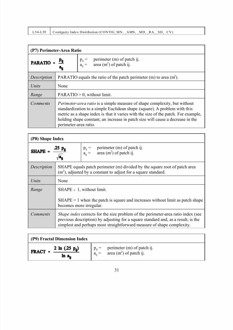
7/14/2019 Bothanical_Metrics
http://slidepdf.com/reader/full/bothanicalmetrics 31/99
31
L54-L59 Contiguity Index Distribution (CONTIG_MN, _AMN, _MD, _RA, _SD, _CV)
(P7) Perimeter-Area Ratio
pij = perimeter (m) of patch ij.aij = area (m2) of patch ij.
Description PARATIO equals the ratio of the patch perimeter (m) to area (m2).
Units None
Range PARATIO > 0, without limit.
Comments Perimeter-area ratio is a simple measure of shape complexity, but without
standardization to a simple Euclidean shape (square). A problem with this
metric as a shape index is that it varies with the size of the patch. For example,holding shape constant, an increase in patch size will cause a decrease in the
perimeter-area ratio.
(P8) Shape Index
pij = perimeter (m) of patch ij.
aij = area (m2) of patch ij.
Description SHAPE equals patch perimeter (m) divided by the square root of patch area
(m2
), adjusted by a constant to adjust for a square standard.
Units None
Range SHAPE $ 1, without limit.
SHAPE = 1 when the patch is square and increases without limit as patch shape
becomes more irregular.
Comments Shape index corrects for the size problem of the perimeter-area ratio index (see
previous description) by adjusting for a square standard and, as a result, is the
simplest and perhaps most straightforward measure of shape complexity.
(P9) Fractal Dimension Index
pij = perimeter (m) of patch ij.
aij = area (m2) of patch ij.
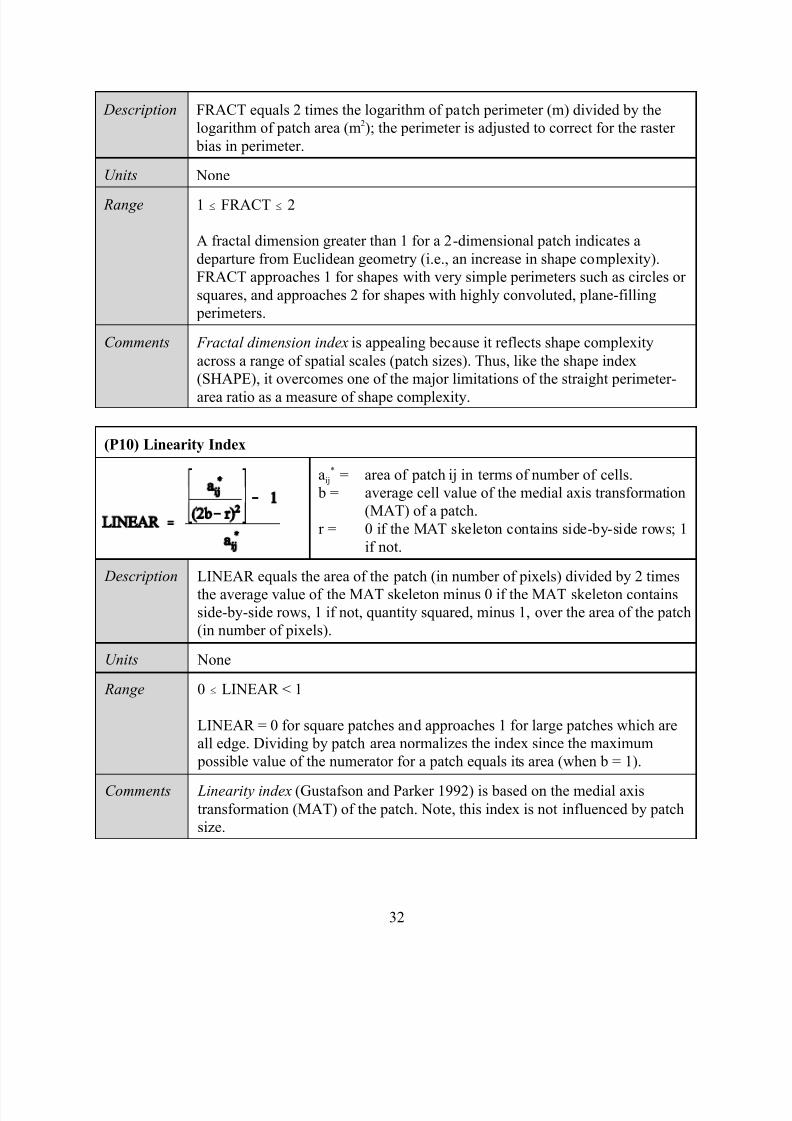
7/14/2019 Bothanical_Metrics
http://slidepdf.com/reader/full/bothanicalmetrics 32/99
32
Description FRACT equals 2 times the logarithm of patch perimeter (m) divided by the
logarithm of patch area (m2); the perimeter is adjusted to correct for the raster
bias in perimeter.
Units None
Range 1 # FRACT # 2
A fractal dimension greater than 1 for a 2-dimensional patch indicates a
departure from Euclidean geometry (i.e., an increase in shape complexity).
FRACT approaches 1 for shapes with very simple perimeters such as circles or
squares, and approaches 2 for shapes with highly convoluted, plane-filling
perimeters.
Comments Fractal dimension index is appealing because it reflects shape complexity
across a range of spatial scales (patch sizes). Thus, like the shape index
(SHAPE), it overcomes one of the major limitations of the straight perimeter-
area ratio as a measure of shape complexity.
(P10) Linearity Index
aij* = area of patch ij in terms of number of cells.
b = average cell value of the medial axis transformation
(MAT) of a patch.
r = 0 if the MAT skeleton contains side-by-side rows; 1
if not.
Description LINEAR equals the area of the patch (in number of pixels) divided by 2 times
the average value of the MAT skeleton minus 0 if the MAT skeleton containsside-by-side rows, 1 if not, quantity squared, minus 1, over the area of the patch
(in number of pixels).
Units None
Range 0 # LINEAR < 1
LINEAR = 0 for square patches and approaches 1 for large patches which are
all edge. Dividing by patch area normalizes the index since the maximum
possible value of the numerator for a patch equals its area (when b = 1).
Comments Linearity index (Gustafson and Parker 1992) is based on the medial axistransformation (MAT) of the patch. Note, this index is not influenced by patch
size.
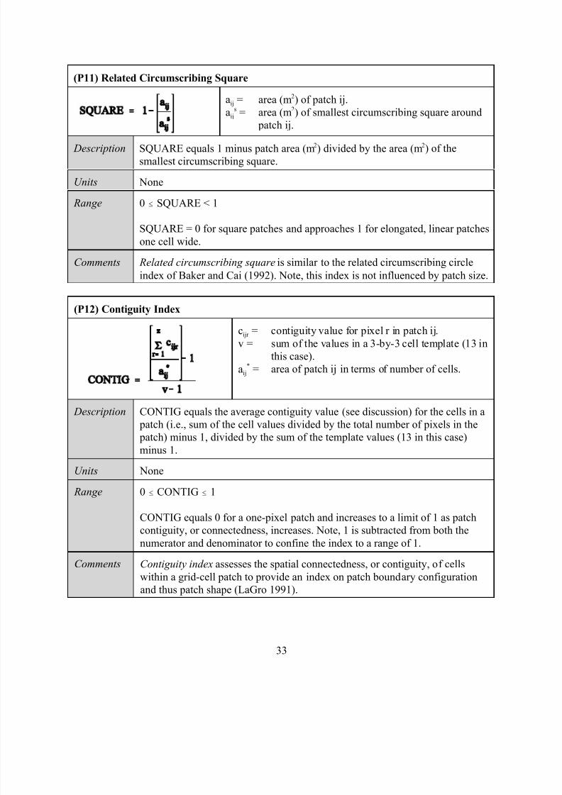
7/14/2019 Bothanical_Metrics
http://slidepdf.com/reader/full/bothanicalmetrics 33/99
33
(P11) Related Circumscribing Square
aij = area (m2) of patch ij.
aijs = area (m2) of smallest circumscribing square around
patch ij.
Description SQUARE equals 1 minus patch area (m2) divided by the area (m2) of the
smallest circumscribing square.
Units None
Range 0 # SQUARE < 1
SQUARE = 0 for square patches and approaches 1 for elongated, linear patches
one cell wide.
Comments Related circumscribing square is similar to the related circumscribing circle
index of Baker and Cai (1992). Note, this index is not influenced by patch size.
(P12) Contiguity Index
cijr = contiguity value for pixel r in patch ij.
v = sum of the values in a 3-by-3 cell template (13 in
this case).
aij
* = area of patch ij in terms of number of cells.
Description CONTIG equals the average contiguity value (see discussion) for the cells in a
patch (i.e., sum of the cell values divided by the total number of pixels in the
patch) minus 1, divided by the sum of the template values (13 in this case)
minus 1.
Units None
Range 0 # CONTIG # 1
CONTIG equals 0 for a one-pixel patch and increases to a limit of 1 as patch
contiguity, or connectedness, increases. Note, 1 is subtracted from both the
numerator and denominator to confine the index to a range of 1.
Comments Contiguity index assesses the spatial connectedness, or contiguity, of cells
within a grid-cell patch to provide an index on patch boundary configuration
and thus patch shape (LaGro 1991).
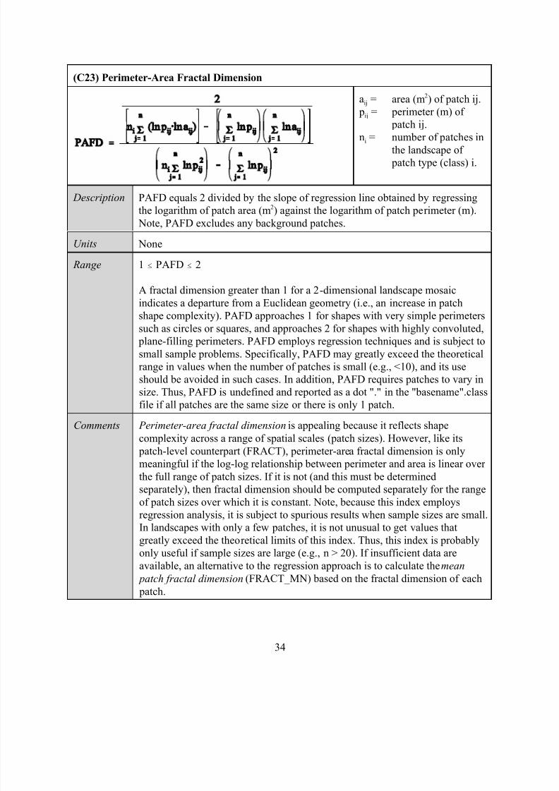
7/14/2019 Bothanical_Metrics
http://slidepdf.com/reader/full/bothanicalmetrics 34/99
34
(C23) Perimeter-Area Fractal Dimension
aij = area (m2) of patch ij.
pij = perimeter (m) of
patch ij.
ni = number of patches inthe landscape of
patch type (class) i.
Description PAFD equals 2 divided by the slope of regression line obtained by regressing
the logarithm of patch area (m2) against the logarithm of patch perimeter (m).
Note, PAFD excludes any background patches.
Units None
Range 1 # PAFD # 2
A fractal dimension greater than 1 for a 2-dimensional landscape mosaic
indicates a departure from a Euclidean geometry (i.e., an increase in patch
shape complexity). PAFD approaches 1 for shapes with very simple perimeters
such as circles or squares, and approaches 2 for shapes with highly convoluted,
plane-filling perimeters. PAFD employs regression techniques and is subject to
small sample problems. Specifically, PAFD may greatly exceed the theoretical
range in values when the number of patches is small (e.g., <10), and its use
should be avoided in such cases. In addition, PAFD requires patches to vary in
size. Thus, PAFD is undefined and reported as a dot "." in the "basename".class
file if all patches are the same size or there is only 1 patch.
Comments Perimeter-area fractal dimension is appealing because it reflects shape
complexity across a range of spatial scales (patch sizes). However, like its
patch-level counterpart (FRACT), perimeter-area fractal dimension is only
meaningful if the log-log relationship between perimeter and area is linear over
the full range of patch sizes. If it is not (and this must be determined
separately), then fractal dimension should be computed separately for the range
of patch sizes over which it is constant. Note, because this index employs
regression analysis, it is subject to spurious results when sample sizes are small.
In landscapes with only a few patches, it is not unusual to get values that
greatly exceed the theoretical limits of this index. Thus, this index is probably
only useful if sample sizes are large (e.g., n > 20). If insufficient data areavailable, an alternative to the regression approach is to calculate the mean
patch fractal dimension (FRACT_MN) based on the fractal dimension of each
patch.
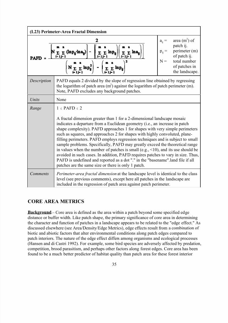
7/14/2019 Bothanical_Metrics
http://slidepdf.com/reader/full/bothanicalmetrics 35/99
35
(L23) Perimeter-Area Fractal Dimension
aij = area (m2) of
patch ij.
pij = perimeter (m)
of patch ij. N = total number
of patches in
the landscape.
Description PAFD equals 2 divided by the slope of regression line obtained by regressing
the logarithm of patch area (m2) against the logarithm of patch perimeter (m).
Note, PAFD excludes any background patches.
Units None
Range 1 # PAFD # 2
A fractal dimension greater than 1 for a 2-dimensional landscape mosaic
indicates a departure from a Euclidean geometry (i.e., an increase in patch
shape complexity). PAFD approaches 1 for shapes with very simple perimeters
such as squares, and approaches 2 for shapes with highly convoluted, plane-
filling perimeters. PAFD employs regression techniques and is subject to small
sample problems. Specifically, PAFD may greatly exceed the theoretical range
in values when the number of patches is small (e.g., <10), and its use should be
avoided in such cases. In addition, PAFD requires patches to vary in size. Thus,
PAFD is undefined and reported as a dot "." in the "basename".land file if all
patches are the same size or there is only 1 patch.
Comments Perimeter-area fractal dimension at the landscape level is identical to the class
level (see previous comments), except here all patches in the landscape are
included in the regression of patch area against patch perimeter.
CORE AREA METRICS
Background.– Core area is defined as the area within a patch beyond some specified edge
distance or buffer width. Like patch shape, the primary significance of core area in determining
the character and function of patches in a landscape appears to be related to the "edge effect." As
discussed elsewhere (see Area/Density/Edge Metrics), edge effects result from a combination of biotic and abiotic factors that alter environmental conditions along patch edges compared to
patch interiors. The nature of the edge effect differs among organisms and ecological processes
(Hansen and di Castri 1992). For example, some bird species are adversely affected by predation,
competition, brood parasitism, and perhaps other factors along forest edges. Core area has been
found to be a much better predictor of habitat quality than patch area for these forest interior
7/14/2019 Bothanical_Metrics
http://slidepdf.com/reader/full/bothanicalmetrics 36/99
36
specialists (Temple 1986). Unlike patch area, core area is affected by patch shape. Thus, while a
patch may be large enough to support a given species, it still may not contain enough suitable
core area to support the species. In some cases, it seems likely that edge effects would vary in
relation to the type and nature of the edge (e.g., the degree of floristic and structural contrast and
orientation). Thus, FRAGSTATS allows the user to specified an edge distance file that contains
edge influence distances for every pairwise combination of patch types. In the absence of suchinformation, the user can specify a single edge width for all edge types. In raster images, there
are different ways to determine core area. FRAGSTATS employs a method in which a cell's 4
parallel neighbors are evaluated for similarity; diagonal neighbors are ignored. This method
tends to slightly over-estimate the true core area. Other methods can seriously under-estimate
core area.
FRAGSTATS Metics.--FRAGSTATS computes several metrics based on core area at the patch,
class, and landscape levels. Most of the indices dealing with number or density of patches, size
of patches, and variability in patch size have corresponding core area indices computed in the
same manner after eliminating the edge or buffer from all patches. For example, patch area, class
area, total landscape area, and the percentage of landscape in each patch type all havecounterparts computed after eliminating edge area defined by the specified edge width; these are
core area (CORE) at the patch level, total core area (TCA) at the class and landscape levels, and
core area percent of landscape (CPLAND) at the class level. The latter index quantifies the core
area in each patch type as a percentage of total landscape area. For organisms strongly associated
with patch interiors, this index may provide a better measure of habitat availability than its
counterpart, percentage of landscape (PLAND). In contrast to their counterparts, these core area
indices integrate into a single measure the affects of patch area, patch shape, and edge effect
distance. Therefore, although they quantify landscape composition, they are affected by
landscape configuration. For this reason, these metrics at the class level may be useful in the
study of habitat loss and fragmentation.
From an organism-centered perspective, a single patch may actually contain several disjunct
patches of suitable interior habitat, and it may be more appropriate to consider disjunct core areas
as separate patches. For this reason, FRAGSTATS computes the number of core areas in each
patch (NCORE), as well as the number in each class and the landscape as a whole (NDCA). If
core area is deemed more important than total area, then these indices may be more applicable
than their counterparts, but they are subject to the same limitations as their counterparts (number
of patches) because they are not standardized with respect to area. For this reason, number of
core areas can be reported on a per unit area basis (disjunct core area density, DCAD) that has
the same ecological applicability as its counterpart (patch density), except that all edge area is
eliminated from consideration. Conversely, this information can be represented as mean core
area (CORE_MN). Like their counterparts, note the difference between core area density andmean core area at the class level. Specifically, core area density is based on total landscape area;
whereas, mean core area is based on total core area for the class. In contrast, at the landscape
level, they are both based on total landscape area and are therefore completely redundant.
Furthermore, mean core area can be defined in 2 ways. First, mean core area can be defined as
the mean core area per patch (CORE_MN). Thus, patches with no core area are included in the
7/14/2019 Bothanical_Metrics
http://slidepdf.com/reader/full/bothanicalmetrics 37/99
37
average, and the total core area in a patch is considered together as 1 observation, regardless of
whether the core area is contiguous or divided into 2 or more disjunct areas within the patch.
Alternatively, mean core area can be defined as the mean area per disjunct core (DCORE_MN).
The distinction between these 2 ways of defining mean core area should be noted.
FRAGSTATS also computes an index that quantifies core area as a percentage of total area. Thecore area index (CAI) at the patch level quantifies the percentage of the patch that is comprised
of core area. Similarly, at the class and landscape levels core area index area-weighted mean
(CAI_AMN) quantifies core area for the entire class or landscape as a percentage of total class or
landscape area, respectively. Note, that this is equivalent to the total core area index reported in
FRAGSTATS 2.0. The core area index is basically an edge-to-interior ratio like many of the
shape indices (see Shape Metrics), the main difference being that the core area index treats edge
as an area of varying width and not as a line (perimeter) around each patch. In addition, the core
area index is a relative measure; it does not reflect patch size, class area, or total landscape area;
it merely quantifies the percentage of available area, regardless of whether it is 10 ha or 1,000 ha,
comprised of core. This index does not confound area and configuration like the previous core
area indices; rather, it isolates the configuration effect. For this reason, the core area index is probably best interpreted in conjunction with total area at the corresponding scale. For example,
in conjunction with total class area, this index could serve as effective fragmentation index for a
particular class.
Limitations.--All core area indices are affected by the interaction of patch size, patch shape, and
the specified edge width. In particular, increasing edge width or shape complexity, or decreasing
patch size will decrease core area, and vice versa. On the one hand, this may be desirable as an
integrative measure that has explicit functional relevance to the organism or process under
consideration. On the other hand, there are potential pitfalls associated with integrative measures
like core area. In particular, the confounding of patch area and configuration effects can
complicate interpretation. For example, if the core area is small, it indicates that very little corearea is available, but it does not discriminate between a small patch (area effect) and a large patch
with a complex shape (configuration effect). In addition, core area is meaningful only if the
specified edge influence distance is meaningful to the phenomenon under investigation.
Unfortunately, in many cases there is no empirical basis for specifying any particular edge
influence distance and so it must be chosen somewhat arbitrarily. The usefulness of core area as a
metric is directly related to the arbitrariness in the specified edge influence distance, and this
should be clearly understood when using these metrics.
Ultimately, the utility of core area metrics compared to their patch area counterparts depends on
the resolution, minimum patch dimensions, and edge influence distance(s) employed. For
example, given a landscape with a resolution of 1 m2 and minimum patch dimensions of 100 x100 m, if an edge influence distance of 1 m is specified, then core area and patch area will be
nearly identical and core area will be relatively insensitive to differences in patch size and shape.
In this case, core area offers little over its patch area counterpart.
7/14/2019 Bothanical_Metrics
http://slidepdf.com/reader/full/bothanicalmetrics 38/99
38
Code Metric (acronym)
Patch Metrics
P13 Core Area (CORE)
P14 Number of Core Areas (NCA)
P15 Core Area Index (CAI)
P16 Average Depth Index (ADEPTH)
P17 Maximum Depth Index (MDEPTH)
Class Metrics
C60 Total Core Area (TCA)
C6 1 C ore Are a P er ce nta ge o f L and sc ap e (C PL AN D)
C62 N umb er of Dis ju nct Co re A re as (N DC A)
C63 D isjun ct C ore A re a D ens it y ( DCA D)
C64-C69 Core Area Distribution (CORE_MN, _AMN, _MD, _RA, _SD, _CV)
C70-C75 Disjunct Core Area Distribution (DCORE_MN, _AMN, _MD, _RA, _SD, _CV)
C76-C81 Core Area Index Distribution (CAI_MN, _AMN, _MD, _RA, _SD, _CV)
Landscape Metrics
L60 Total Core Area (TCA)
L62 N um ber of Dis ju nct Co re A reas (N DC A)
L63 D isj un ct Co re A re a D ens it y ( DCA D)
L64-L69 Core Area Distribution (CORE_MN, _AMN, _MD, _RA, _SD, _CV)
L70-L75 Disjunct Core Area Distribution (DCORE_MN, _AMN, _MD, _RA, _SD, _CV)
L76-L81 Core Area Index Distribution (CAI_MN, _AMN, _MD, _RA, _SD, _CV)
(P13) Core Area
aijc = core area (m2) of patch ij based on specified buffer
width (m).
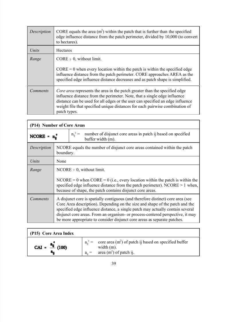
7/14/2019 Bothanical_Metrics
http://slidepdf.com/reader/full/bothanicalmetrics 39/99
39
Description CORE equals the area (m2) within the patch that is further than the specified
edge influence distance from the patch perimeter, divided by 10,000 (to convert
to hectares).
Units Hectares
Range CORE $ 0, without limit.
CORE = 0 when every location within the patch is within the specified edge
influence distance from the patch perimeter. CORE approaches AREA as the
specified edge influence distance decreases and as patch shape is simplified.
Comments Core area represents the area in the patch greater than the specified edge
influence distance from the perimeter. Note, that a single edge influence
distance can be used for all edges or the user can specified an edge influence
weight file that specified unique distances for each pairwise combination of
patch types.
(P14) Number of Core Areas
nijc = number of disjunct core areas in patch ij based on specified
buffer width (m).
Description NCORE equals the number of disjunct core areas contained within the patch
boundary.
Units None
Range NCORE $ 0, without limit.
NCORE = 0 when CORE = 0 (i.e., every location within the patch is within the
specified edge influence distance from the patch perimeter). NCORE > 1 when,
because of shape, the patch contains disjunct core areas.
Comments A disjunct core is spatially contiguous (and therefore distinct) core area (see
Core Area description). Depending on the size and shape of the patch and the
specified edge influence distance, a single patch may actually contain several
disjunct core areas. From an organism- or process-centered perspective, it may
be more appropriate to consider disjunct core areas as separate patches.
(P15) Core Area Index
aij
c = core area (m2) of patch ij based on specified buffer
width (m).
aij = area (m2) of patch ij.

7/14/2019 Bothanical_Metrics
http://slidepdf.com/reader/full/bothanicalmetrics 40/99
40
Description CAI equals the patch core area (m2) divided by total patch area (m2), multiplied
by 100 (to convert to a percentage); in other words, CAI equals the percentage
of a patch that is core area.
Units Percent
Range 0 # CAI < 100
CAI = 0 when CORE = 0 (i.e., every location within the patch is within the
specified edge influence distance from the patch perimeter); that is, when the
patch contains no core area. CAI approaches 100 when the patch, because of
size, shape, and edge width, contains mostly core area.
Comments Core area index is a relative index that quantifies core area as a percentage of
patch area (i.e., the percentage of the patch that is comprised of core area).
(P16) Average Depth Index
Description ADEPTH equals the average value of the MAT skeleton (in number of cells)
times the cell size (m) minus the cell size (m). The subtraction is necessary to
adjust the minimum value to zero for an average MAT of 1 cell.
Units Meters
Range ADEPTH > 0, without limit.
ADEPTH = 0 for a linear patch one cell wide. Here, every cell in the patchwould be on the edge and therefore the patch would have no depth. ADEPTH
increases as the patch increases in size and becomes more Euclidean in shape.
Comments Average depth index (Gustafson and Parker 1992) is based on the medial axis
transformation (MAT) of the patch (see Linearity Index description). The
average depth index is based on the fact that elongated patches of a given area
have MAT skeletons closer to their edges (and therefore a smaller average
distance) than square patches of the same area. Here, we compute the index in
terms of absolute distance (meters) rather than number of cells, to give the
index more direct interpretive value. The average depth index represents the
average depth to the core of the patch and is therefore sensitive to both patchsize and shape. Holding shape constant, larger patches will have greater average
depth to the MAT. Similarly, holding area constant, more compact and
Euclidean shapes will have greater average depth to the MAT.
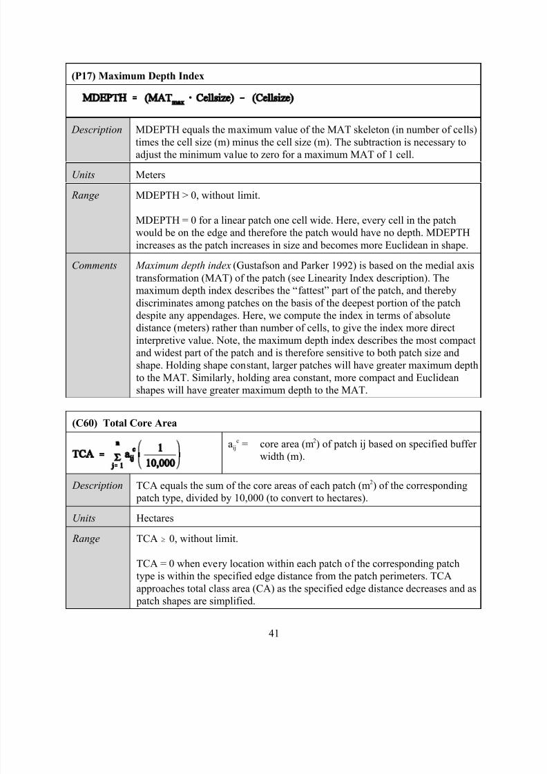
7/14/2019 Bothanical_Metrics
http://slidepdf.com/reader/full/bothanicalmetrics 41/99
41
(P17) Maximum Depth Index
Description MDEPTH equals the maximum value of the MAT skeleton (in number of cells)
times the cell size (m) minus the cell size (m). The subtraction is necessary to
adjust the minimum value to zero for a maximum MAT of 1 cell.
Units Meters
Range MDEPTH > 0, without limit.
MDEPTH = 0 for a linear patch one cell wide. Here, every cell in the patch
would be on the edge and therefore the patch would have no depth. MDEPTH
increases as the patch increases in size and becomes more Euclidean in shape.
Comments Maximum depth index (Gustafson and Parker 1992) is based on the medial axis
transformation (MAT) of the patch (see Linearity Index description). The
maximum depth index describes the “fattest” part of the patch, and thereby
discriminates among patches on the basis of the deepest portion of the patch
despite any appendages. Here, we compute the index in terms of absolute
distance (meters) rather than number of cells, to give the index more direct
interpretive value. Note, the maximum depth index describes the most compact
and widest part of the patch and is therefore sensitive to both patch size and
shape. Holding shape constant, larger patches will have greater maximum depth
to the MAT. Similarly, holding area constant, more compact and Euclidean
shapes will have greater maximum depth to the MAT.
(C60) Total Core Area
aijc = core area (m2) of patch ij based on specified buffer
width (m).
Description TCA equals the sum of the core areas of each patch (m2) of the corresponding
patch type, divided by 10,000 (to convert to hectares).
Units Hectares
Range TCA$
0, without limit.
TCA = 0 when every location within each patch of the corresponding patch
type is within the specified edge distance from the patch perimeters. TCA
approaches total class area (CA) as the specified edge distance decreases and as
patch shapes are simplified.
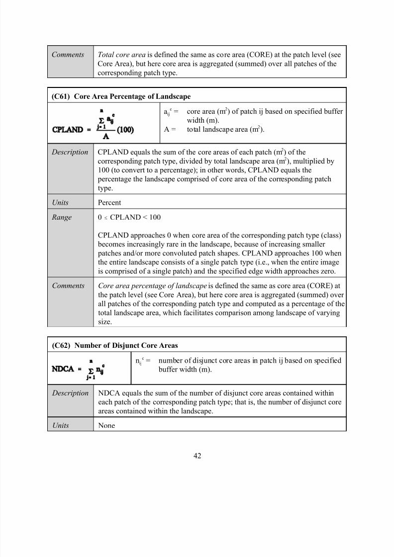
7/14/2019 Bothanical_Metrics
http://slidepdf.com/reader/full/bothanicalmetrics 42/99
42
Comments Total core area is defined the same as core area (CORE) at the patch level (see
Core Area), but here core area is aggregated (summed) over all patches of the
corresponding patch type.
(C61) Core Area Percentage of Landscape
aijc = core area (m2) of patch ij based on specified buffer
width (m).
A = total landscape area (m2).
Description CPLAND equals the sum of the core areas of each patch (m2) of the
corresponding patch type, divided by total landscape area (m2), multiplied by
100 (to convert to a percentage); in other words, CPLAND equals the
percentage the landscape comprised of core area of the corresponding patch
type.
Units Percent
Range 0 # CPLAND < 100
CPLAND approaches 0 when core area of the corresponding patch type (class)
becomes increasingly rare in the landscape, because of increasing smaller
patches and/or more convoluted patch shapes. CPLAND approaches 100 when
the entire landscape consists of a single patch type (i.e., when the entire image
is comprised of a single patch) and the specified edge width approaches zero.
Comments Core area percentage of landscape is defined the same as core area (CORE) at
the patch level (see Core Area), but here core area is aggregated (summed) over all patches of the corresponding patch type and computed as a percentage of the
total landscape area, which facilitates comparison among landscape of varying
size.
(C62) Number of Disjunct Core Areas
nijc = number of disjunct core areas in patch ij based on specified
buffer width (m).
Description NDCA equals the sum of the number of disjunct core areas contained withineach patch of the corresponding patch type; that is, the number of disjunct core
areas contained within the landscape.
Units None
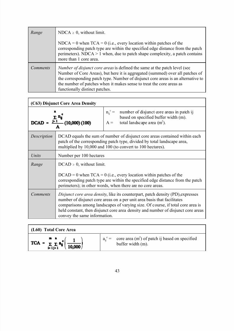
7/14/2019 Bothanical_Metrics
http://slidepdf.com/reader/full/bothanicalmetrics 43/99
43
Range NDCA $ 0, without limit.
NDCA = 0 when TCA = 0 (i.e., every location within patches of the
corresponding patch type are within the specified edge distance from the patch
perimeters). NDCA > 1 when, due to patch shape complexity, a patch contains
more than 1 core area.
Comments Number of disjunct core areas is defined the same at the patch level (see
Number of Core Areas), but here it is aggregated (summed) over all patches of
the corresponding patch type. Number of disjunct core areas is an alternative to
the number of patches when it makes sense to treat the core areas as
functionally distinct patches.
(C63) Disjunct Core Area Density
nijc = number of disjunct core areas in patch ij
based on specified buffer width (m).A = total landscape area (m2).
Description DCAD equals the sum of number of disjunct core areas contained within each
patch of the corresponding patch type, divided by total landscape area,
multiplied by 10,000 and 100 (to convert to 100 hectares).
Units Number per 100 hectares
Range DCAD $ 0, without limit.
DCAD = 0 when TCA = 0 (i.e., every location within patches of thecorresponding patch type are within the specified edge distance from the patch
perimeters); in other words, when there are no core areas.
Comments Disjunct core area density, like its counterpart, patch density (PD),expresses
number of disjunct core areas on a per unit area basis that facilitates
comparisons among landscapes of varying size. Of course, if total core area is
held constant, then disjunct core area density and number of disjunct core areas
convey the same information.
(L60) Total Core Areaaij
c = core area (m2) of patch ij based on specified
buffer width (m).
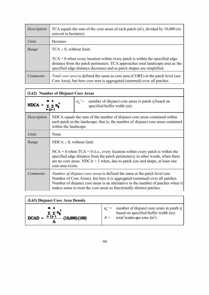
7/14/2019 Bothanical_Metrics
http://slidepdf.com/reader/full/bothanicalmetrics 44/99
44
Description TCA equals the sum of the core areas of each patch (m2), divided by 10,000 (to
convert to hectares).
Units Hectares
Range TCA $ 0, without limit.
TCA = 0 when every location within every patch is within the specified edge
distance from the patch perimeters. TCA approaches total landscape area as the
specified edge distance decreases and as patch shapes are simplified.
Comments Total core area is defined the same as core area (CORE) at the patch level (see
Core Area), but here core area is aggregated (summed) over all patches.
(L62) Number of Disjunct Core Areas
nij
c = number of disjunct core areas in patch ij based on
specified buffer width (m).
Description NDCA equals the sum of the number of disjunct core areas contained within
each patch in the landscape; that is, the number of disjunct core areas contained
within the landscape.
Units None
Range NDCA $ 0, without limit.
NCA = 0 when TCA = 0 (i.e., every location within every patch is within the
specified edge distance from the patch perimeters); in other words, when thereare no core areas. NDCA > 1 when, due to patch size and shape, at least one
core area exists.
Comments Number of disjunct core areas is defined the same at the patch level (see
Number of Core Areas), but here it is aggregated (summed) over all patches.
Number of disjunct core areas is an alternative to the number of patches when it
makes sense to treat the core areas as functionally distinct patches.
(L63) Disjunct Core Area Density
nijc = number of disjunct core areas in patch ij
based on specified buffer width (m).
A = total landscape area (m2).
7/14/2019 Bothanical_Metrics
http://slidepdf.com/reader/full/bothanicalmetrics 45/99
45
Description DCAD equals the sum of number of disjunct core areas contained within each
patch, divided by total landscape area, multiplied by 10,000 and 100 (to convert
to 100 hectares).
Units Number per 100 hectares
Range DCAD $ 0, without limit.
DCAD = 0 when TCA = 0 (i.e., every location within every patch is within the
specified edge distance from the patch perimeters); in other words, when there
are no core areas. DCAD > 1 when, due to patch size and shape, at least one
core area exists.
Comments Disjunct core area density, like its counterpart, patch density (PD),expresses
number of disjunct core areas on a per unit area basis that facilitates
comparisons among landscapes of varying size. Of course, if total core area is
held constant, then disjunct core area density and number of disjunct core areas
convey the same information.
ISOLATION/PROXIMITY METRICS
Background.--Isolation deals explicitly with the spatial and temporal context of habitat patches,
rather than the spatial character of the patches themselves. Isolation of habitat patches is a critical
factor in the dynamics of spatially structured populations. For example, there has been a
proliferation of mathematical models on population dynamics and species interactions in
spatially subdivided populations (Kareiva 1990), and results suggest that the dynamics of local
plant and animal populations in a patch are influenced by their proximity to other subpopulationsof the same or competing species. Patch isolation plays a critical role in island biogeographic
theory (MacArthur and Wilson 1967) and metapopulation theory (Levins 1970, Gilpin and
Hanski 1991). The role of patch isolation (e.g., as measured by interpatch distance) in
metapopulations has had a preeminent role in conservation efforts for endangered species (e.g.,
Lamberson et al. 1992, McKelvey et al. 1992).
Isolation is particularly important in the context of habitat fragmentation. Several authors have
claimed, for example, that patch isolation explains why fragmented habitats often contain fewer
bird species than contiguous habitats (Moore and Hooper 1975, Forman et al. 1976, Helliwell
1976, Whitcomb et al. 1981, Hayden et al. 1985, Dickman 1987). Specifically, as habitat is lost
and fragmented, residual habitat patches become more isolated from each other in space andtime. One of the more immediate consequence of this is the disruption of movement patterns and
the resulting isolation of individuals and local populations. This has important metapopulation
consequences. As habitat is fragmented, it is broken up into remnants that are isolated to varying
degrees. Because remnant habitat patches are relatively small and therefore support fewer
individuals, there will be fewer local (within patch) opportunities for intra-specific interactions.
7/14/2019 Bothanical_Metrics
http://slidepdf.com/reader/full/bothanicalmetrics 46/99
46
This may not present a problem for individuals (and the persistence of the population) if
movement among patches is largely unimpeded by intervening habitats in the matrix and
connectivity across the landscape can be maintained. However, if movement among habitat
patches is significantly impeded or prevented, then individuals (and local populations) in
remnant habitat patches may become functionally isolated. The degree of isolation for any
fragmented habitat distribution will vary among species depending on how they perceive andinteract with landscape patterns (Dale et al. 1994, With and Crist 1995, Pearson et al. 1996, With
et al. 1997, With 1999); less vagile species with very restrictive habitat requirements and limited
gap-crossing ability will likely be most sensitive to isolation effects.
Habitat patches can become functionally isolated in several ways. First, the patch edge may act
as a filter or barrier that impedes or prevents movement, thereby disrupting emigration and
dispersal from the patch (Wiens et al. 1985). Some evidence for this exists for small mammals
(e.g., Wegner and Merriam 1979, Chasko and Gates 1982, Bendell and Gates 1987, Yahner
1986), but the data are scarce for other vertebrates. Whether edges themselves can limit
movement presumably depends on what species are trying to cross the edge and on the structure
of the edge habitat (Kremsater and Bunnell 1999). Second, the distance from remnant habitat patches to other neighboring habitat patches may influence the likelihood of successful
movement of individuals among habitat patches. Again, the distance at which movement rates
significantly decline will vary among species depending on how they scale the environment. In
general, larger organisms can travel longer distances. Therefore, a 100 m-wide agricultural field
may be a complete barrier to dispersal for small organisms such as invertebrates (e.g., Mader
1984), yet be quite permeable for larger and more vagile organisms such as birds. Lastly, the
composition and structure of the intervening landscape mosaic may determine the permeability
of the landscape to movements. Note that under an island biogeographic perspective, habitat
patches exist in a uniform sea that is hostile to both survival and dispersal. In this case, the
matrix is presumed to contain no meaningful structure and isolation is influenced largely by the
distance among favorable habitat patches. However, under a landscape mosaic perspective,habitat patches are bounded by other patches that may be more or less similar (as opposed to
highly contrasting and hostile) and connectivity is assessed by the extent to which movement is
facilitated or impeded through different habitat types across the landscape. Each habitat may
differ in its “viscosity” or resistance to movement, facilitating movement through certain
elements of the landscape and impeding it in others. Again, the degree to which a given
landscape structure facilitates or impedes movement will vary among organisms. Regardless of
how habitat patches become isolated, whether it be due to properties of the edges themselves, the
distance between patches, or properties of the intervening matrix, the end result is the
same–fewer individual movements among habitat patches.
Unfortunately, because of the many factors that influence the functional isolation of a patch, it isa difficult thing to capture in a single measure. In the context of fragmentation, isolation can be
measured as the time since the habitat was physically subdivided, but this is fraught with
practical difficulties. For example, rarely do we have accurate historical data from which to
determine when each patch was isolated. Moreover, given that fragmentation is an ongoing
process, it can be difficult to objectively determine at what point the habitat becomes subdivided,
7/14/2019 Bothanical_Metrics
http://slidepdf.com/reader/full/bothanicalmetrics 47/99
47
since this is largely a function of scale. Isolation can be measured in the spatial dimension in
several ways, depending on how one views the concept of isolation. The simplest measures are
based on Euclidean distance between nearest neighbors (McGarigal and Marks 1995) or the
cumulative area of neighboring habitat patches (weighted by nearest neighbor distance) within
some ecological neighborhood (Gustafson and Parker 1992). These measures adopt an island
biogeographic perspective, as they treat the landscape as a binary mosaic consisting of habitat patches and uniform matrix. Thus, the context of a patch is defined by the proximity and area of
neighboring habitat patches; the role of the matrix is ignored. However, these measures can be
modified to take into account other habitat types in the so-called matrix and their affects on the
insularity of the focal habitat. For example, simple Euclidean distance can be modified to
account for functional differences among organisms. The functional distance between patches
clearly depends on how each organism scales and interacts with landscape patterns (With 1999);
in other words, the same gap between patches may not be perceived as a relevant disconnection
for some organisms, but may be an impassable barrier for others. Similarly, the matrix can be
treated as a mosaic of patch types that contribute differentially to the isolation of the focal
habitat. For example, isolation can be measured by the degree of contrast (i.e., the magnitude of
differences in one or more attributes between adjacent patch types) between the focal habitat andneighboring patches.
FRAGSTATS Metrics.--FRAGSTATS computes several isolation metrics based on nearest-
neighbor distance at the patch, class, and landscape levels. Nearest-neighbor distance is defined
as the distance from a patch to a neighboring patch of the same or different class, based on edge-
to-edge distance. These metrics are all fundamentally patch-level metrics (i.e., measured for each
patch) that can be summarized at the class or landscape levels. FRAGSTATS computes two
metrics that adopt an island biogeographic perspective on patch isolation: (1) Euclidean nearest
neighbor distance and (2) proximity index. Euclidean nearest neighbor distance (ENN) is
perhaps the simplest measure of patch context and has been used extensively to quantify patch
isolation. Here, nearest neighbor distance is defined using simple Euclidean geometry as theshortest straight-line distance between the focal patch and its nearest neighbor of the same class.
Even though nearest neighbor distance is often used to evaluate patch isolation, it is important to
recognize that the single nearest patch may not fully represent the ecological neighborhood of the
focal patch. For example, a neighboring patch 100 m away that is 1 ha is size may not be as
important to the effective isolation of the focal patch as a neighboring patch 200 m away, but
1000 ha is size. To overcome this limitation, the proximity index (PROXIM) was developed by
Gustafson and Parker (1992)[see also Gustafson and Parker 1994, Gustafson et al. 1994,
Whitcomb et al. 1981]. This index considers the size and proximity of all patches whose edges
are within a specified search radius of the focal patch. The index is computed as the sum, over all
patches of the corresponding patch type whose edges are within the search radius of the focal
patch, of each patch size divided by the square of its distance from the focal patch. Note thatFRAGSTATS uses the distance between the focal patch and each of the other patches within the
search radius, similar to the isolation index of Whitcomb et al. (1981), rather than the nearest-
neighbor distance of each patch within the search radius (which could be to a patch other than the
focal patch), as in Gustafson and Parker (1992). The proximity index quantifies the spatial
context of a (habitat) patch in relation to its neighbors of the same class; specifically, the index
7/14/2019 Bothanical_Metrics
http://slidepdf.com/reader/full/bothanicalmetrics 48/99
48
distinguishes sparse distributions of small habitat patches from configurations where the habitat
forms a complex cluster of larger patches. All other things being equal, a patch located in a
neighborhood (defined by the search radius) containing more of the corresponding patch type
than another patch will have a larger index value. Similarly, all other things being equal, a patch
located in a neighborhood in which the corresponding patch type is distributed in larger, more
contiguous, and/or closer patches than another patch will have a larger index value. Thus, the proximity index measures both the degree of patch isolation and the degree of fragmentation of
the corresponding patch type within the specified neighborhood of the focal patch.
At the class and landscape levels, FRAGSTATS computes several distribution statistics
associated with the Euclidean nearest neighbor distance and proximity index. At the class level,
the mean proximity index measures the degree of isolation and fragmentation of the
corresponding patch type and the performance of the index under various scenarios is described
in detail by Gustafson and Parker (1994). FRAGSTATS also summarizes the proximity index at
the landscape level by aggregating across all patches in the landscape, although the performance
of this index as a measure of overall landscape pattern has not been evaluated quantitatively.
Similarly, at the class and landscape levels, FRAGSTATS computes the mean and variability inEuclidean nearest neighbor distance. At the class level, mean nearest-neighbor distance can only
be computed if there are at least 2 patches of the corresponding type. At the landscape level,
mean nearest-neighbor distance considers only patches that have neighbors. Thus, there could be
10 patches in the landscape, but 8 of them might belong to separate patch types and therefore
have no neighbor within the landscape. In this case, mean nearest-neighbor distance would be
based on the distance between the 2 patches of the same type. These 2 patches could be close
together or far apart. In either case, the mean nearest-neighbor distance for this landscape may
not characterize the entire landscape very well. For this reason, these metrics should be
interpreted carefully when landscapes contain rare patch types.
In addition to these first-order statistics, the variability in nearest-neighbor distance measures akey aspect of landscape heterogeneity. Specifically, the standard deviation (SD)in Euclidean
nearest neighbor distance (ENN_SD) is a measure of patch dispersion; a small SD relative to the
mean implies a fairly uniform or regular distribution of patches across landscapes, whereas a
large SD relative to the mean implies a more irregular or uneven distribution of patches. The
distribution of patches may reflect underlying natural processes or human-caused disturbance
patterns. In absolute terms, the magnitude of nearest-neighbor SD is a function of the mean
nearest-neighbor distance and variation in nearest-neighbor distance among patches. Thus, while
SD does convey information about nearest neighbor variability, it is a difficult parameter to
interpret without doing so in conjunction with the mean nearest-neighbor distance. For example,
2 landscapes may have the same nearest-neighbor SD, e.g., 100 m; yet 1 landscape may have a
mean nearest-neighbor distance of 100 m, while the other may have a mean nearest-neighbor distance of 1,000 m. In this case, the interpretations of landscape pattern would be very different,
even though the absolute variation is the same. Specifically, the former landscape has a more
irregular but concentrated pattern of patches, while the latter has a more regular but dispersed
pattern of patches. For these reasons, coefficient of variation (CV) often is preferable to SD for
comparing variability among landscapes. Coefficient of variation measures relative variability
7/14/2019 Bothanical_Metrics
http://slidepdf.com/reader/full/bothanicalmetrics 49/99
49
about the mean (i.e., variability as a percentage of the mean), not absolute variability. Thus, it is
not necessary to know the mean nearest-neighbor distance to interpret this metric. Even so,
nearest-neighbor CV can be misleading with regards to landscape structure without also knowing
the number of patches or patch density and other structural characteristics. For example, 2
landscapes may have the same nearest-neighbor CV, e.g., 100%; yet 1 landscape may have 100
patches with a mean nearest-neighbor distance of 100 m, while the other may have 10 patcheswith a mean nearest-neighbor distance of 1,000 m. In this case, the interpretations of overall
landscape pattern could be very different, even though nearest-neighbor CV is the same;
although the identical CV’s indicate that both landscapes have the same regularity or uniformity
in patch distribution. Finally, both SD and CV assume a normal distribution about the mean. In a
real landscape, nearest-neighbor distribution may be highly irregular. In this case, it may be more
informative to inspect the actual distribution itself (e.g., plot a histogram of the nearest neighbor
distances for the corresponding patches), rather than relying on summary statistics such as SD
and CV that make assumptions about the distribution and therefore can be misleading.
FRAGSTATS computes two isolation metrics that adopt a landscape mosaic perspective on
patch isolation: (1) functional nearest neighbor distance and (2) similarity index. Similarity index(SIMILAR) is a modification of the proximity index, the difference being that similarity
considers the size and proximity of all patches, regardless of class, whose edges are within a
specified search radius of the focal patch. The similarity index quantifies the spatial context of a
(habitat) patch in relation to its neighbors of the same or similar class; specifically, the index
distinguishes sparse distributions of small and insular habitat patches from configurations where
the habitat forms a complex cluster of larger, hospitable (i.e., similar) patches. All other things
being equal, a patch located in a neighborhood (defined by the search radius) deemed more
similar (i.e., containing greater area in patches with high similarity) than another patch will have
a larger index value. Similarly, all other things being equal, a patch located in a neighborhood in
which the similar patches are distributed in larger, more contiguous, and/or closer patches than
another patch will have a larger index value. Essentially, the similarity index performs much thesame way as the proximity index, but instead of focusing on only a single patch type (i.e., island
biogeographic perspective), it considers all patch types in the mosaic (i.e., landscape mosaic
perspective). Thus, the similarity index is a more comprehensive measure of patch isolation than
the proximity index for organisms and processes that perceive and respond to patch types
differentially.
Similarly, functional nearest-neighbor distance accounts for one of the major shortcomings of
using Euclidean distance to assess ecological relationships; namely, that the shortest geographic
distance may not be the shortest ecological distance as perceived by an organism or process. The
character of the intervening landscape can significantly alter the rate of flow of the organism or
process of interest. Therefore, it may be more meaningful to assess distance using a least cost patch approach. Here, the distance across a cell is weighted by the degree of resistence it offers to
the ecological flow of interest. Thus, the functional distance between two patches is increased
proportionate the degree of resistance in the intervening landscape.
7/14/2019 Bothanical_Metrics
http://slidepdf.com/reader/full/bothanicalmetrics 50/99
50
Limitations.--There are significant limitations associated with the use of isolation metrics that
must be understood before they are used. The most important limitation of these particular
metrics is that nearest-neighbor distances are computed solely from patches contained within the
landscape boundary. If the landscape extent is small relative to the scale of the organism or
ecological processes under consideration and the landscape is an "open" system relative to that
organism or process, then nearest-neighbor results can be misleading. For example, consider asmall subpopulation of a bird species occupying a patch near the boundary of a somewhat
arbitrarily defined (from a bird's perspective) landscape. The nearest neighbor within the
landscape boundary might be quite far away, yet in reality the closest patch might be very close,
but just outside the designated landscape boundary. The magnitude of this problem is a function
of scale. Increasing the size of the landscape relative to the scale at which the organism under
investigation perceives and responds to the environment will decrease the severity of this
problem.
Similarly, the proximity and similarity indices involve a search window around the focal patch.
Thus, these metrics may be biased low for patches located within the search radius distance from
the landscape boundary because a portion of the search area will be outside the area under consideration. The magnitude is of this problem is also a function of scale. Increasing the size of
the landscape relative to the average patch size and/or decreasing the search radius will decrease
the severity of this problem at the class and landscape levels. However, at the patch level,
regardless of scale, individual patches located within the search radius of the boundary will have
a biased indices. In addition, these indices evaluate the landscape context of patches at a specific
scale of analysis defined by the size of the search radius. Therefore, these indices are only
meaningful if the specified search radius has some ecological relevance to the phenomenon under
consideration. Otherwise, the results will be arbitrary and therefore meaningless.
Lastly, functional nearest-neighbor distance and the similarity index are functional metrics in that
they require additional parameterization, in this case resistance coefficients that are unique to theecological phenomenon under consideration. Consequently, as with any functional metric, their
relevance depends entirely on the meaningfulness of the resistance coefficients applied. If these
are arbitrary assignments or based on weak observational data, results will be arbitrary and
therefore meaningless.
Code Metric (acronym)
Patch Metrics
P18 Proximity Index (PROXIM)
P19 Similarity Index (SIMILAR)
P20 Euclidean Nearest Neighbor Distance (ENN)
P21 Functional Nearest Neighbor Distance (FNN)
Class Metrics
7/14/2019 Bothanical_Metrics
http://slidepdf.com/reader/full/bothanicalmetrics 51/99
51
C82-C87 Proximity Index Distribution (PROXIM_MN, _AMN, _MD, _RA, _SD, _CV)
C88-C93 Similari ty Index Distribution (SIMILAR_MN, _AMN, _MD, _RA, _SD, _CV)
C94-C99 Euclidean Nearest Neighbor Distance Distribution (NNE_MN, _AMN, _MD, _RA, _SD, _CV)
C100-C105 Functional Nearest Neighbor Distance Distribution (NNF_MN, _AMN, _MD, _RA, _SD, _CV)
Landscape Metrics
L82-L87 Proximity Index Distribution (PROXIM_MN, _AMN, _MD, _RA, _SD, _CV)
L88-L93 Similari ty Index Distribution (SIMILAR_MN, _AMN, _MD, _RA, _SD, _CV)
L94-L99 Euclidean Nearest Neighbor Distance Distribution (NNE_MN, _AMN, _MD, _RA, _SD, _CV)
L100-L105 Functional Nearest Neighbor Distance Distribution (NNF_MN, _AMN, _MD, _RA, _SD, _CV)
(P18) Proximity Index
aijs = area (m2) of patch ijs within specified neighborhood
(m) of patch ij.
hijs = distance (m) between patch ijs and patch ijs, based on
patch edge-to-edge distance.
Description PROXIM equals the sum of patch area (m2) divided by the nearest edge-to-edge
distance squared (m2) between the patch and the focal patch of all patches of the
corresponding patch type whose edges are within a specified distance (m) of the
focal patch. Note, when the search buffer extends beyond the landscape
boundary, only patches contained within the landscape are considered in the
computations. In addition, note that the edge-to-edge distances are from cellcenter to cell center.
Units None
Range PROXIM $ 0.
PROXIM = 0 if a patch has no neighbors of the same patch type within the
specified search radius. PROXIM increases as the neighborhood (defined by
the specified search radius) is increasingly occupied by patches of the same
type and as those patches become closer and more contiguous and less
fragmented in distribution. The upper limit of PROXIM is affected by the
search radius and minimum distance between patches.
7/14/2019 Bothanical_Metrics
http://slidepdf.com/reader/full/bothanicalmetrics 52/99
52
Comments Proximity index was developed by Gustafson and Parker (1992) and considers
the size and proximity of all patches whose edges are within a specified search
radius of the focal patch. Note that FRAGSTATS uses the distance between the
focal patch and each of the other patches within the search radius, similar to the
isolation index of Whitcomb et al. (1981), rather than the nearest-neighbor
distance of each patch within the search radius (which could be to a patch other than the focal patch), as in Gustafson and Parker (1992). The index is
dimensionless (i.e., has no units) and therefore the absolute value of the index
has little interpretive value; instead it is used as a comparative index.
(P19) Similarity Index
aijs = area (m2) of patch ijs within specified neighborhood
(m) of patch ij.
dik = similarity between patch types i and k.
hijs = distance (m) between patch ijs and patch ijs, based on patch edge-to-edge distance.
Description SIMILAR equals the sum, over all neighboring patches with edges within a
specified distance (m) of the focal patch, of neighboring patch area (m2) times a
similarity coefficient between the focal patch type and the class of the
neighboring patch (0-1), divided by the nearest edge-to-edge distance squared
(m2) between the focal patch and the neighboring patch. Note, when the search
buffer extends beyond the landscape boundary, only patches contained within
the landscape are considered in the computations. In addition, note that the
edge-to-edge distances are from cell center to cell center.
Units None
Range SIMILAR $ 0
SIMILAR = 0 if all the patches within the specified neighborhood have a zero
similarity coefficient. SIMILAR increases as the neighborhood (defined by the
specified search radius) is increasingly occupied by patches with greater
similarity coefficients and as those similar patches become closer and more
contiguous and less fragmented in distribution.The upper limit of SIMILAR is
affected by the search radius and minimum distance between patches.
Comments Similarity index is a modification of the proximity index (see Proximity Index
description), the difference being that similarity considers the size and
proximity of all patches, regardless of class, whose edges are within a specified
search radius of the focal patch. Like the proximity index, this index is
dimensionless (i.e., has no units) and therefore the absolute value of the index
has little interpretive value; instead it is used as a comparative index.
7/14/2019 Bothanical_Metrics
http://slidepdf.com/reader/full/bothanicalmetrics 53/99
53
(P20) Euclidean Nearest-Neighbor Distance
hij = distance (m) from patch ij to nearest neighboring patch of the
same type (class), based on patch edge-to-edge distance.
Description ENN equals the distance (m) to the nearest neighboring patch of the same type,
based on shortest edge-to-edge distance. Note that the edge-to-edge distances
are from cell center to cell center.
Units Meters
Range ENN > 0, without limit.
Comments Euclidean nearest-neighbor distance is perhaps the simplest measure of patch
context and has been used extensively to quantify patch isolation. Here, nearest
neighbor distance is defined using simple Euclidean geometry as the shortest
straight-line distance between the focal patch and its nearest neighbor of thesame class.
(P21) Functional Nearest-Neighbor Distance
hij* =distance (m) from patch ij to its nearest neighboring patch of the
same type (class), based on least cost path edge-to-edge distance.
Description FNN equals the distance (m) to the nearest neighboring patch of the same type,
based on the least cost path edge-to-edge distance. Note that the edge-to-edge
distances are from cell center to cell center.
Units Meters
Range FNF > 0, without limit.
Comments Functional nearest-neighbor distance accounts for one of the major
shortcomings of using Euclidean distance to assess ecological relationships;
namely, that the shortest geographic distance may not be the shortest ecological
distance as perceived by an organism or process.
CONTRAST METRICS
Background..--Contrast refers to the magnitude of difference between adjacent patch types with
respect to one or more ecological attributes at a given scale that are relevant to the organism or
process under consideration. The contrast between a patch and its neighborhood can influence a
number of important ecological processes (Forman and Godron 1986). The "edge effects"
described elsewhere (see Area/Density/Edge Metrics), for example, are influenced by the degree
7/14/2019 Bothanical_Metrics
http://slidepdf.com/reader/full/bothanicalmetrics 54/99
54
of contrast between patches. Microclimatic changes (e.g., wind, light intensity and quality, etc.)
are likely to extend farther into a patch along an edge with high structural contrast than along an
edge with low structural contrast (Ranney et al. 1981). Similarly, the adverse affects of brown-
headed cowbird nest parasitism on some forest-dwelling neotropical migratory bird species are
likely to be greatest along high-contrast forest edges (e.g., between mature forest patches and
grassland), because cowbirds prefer to forage in early-seral habitats and parasitize nests in late-seral habitats (Brittingham and Temple 1983). In addition, patch isolation may be a function of
the contrast between a patch and its ecological neighborhood. In particular, the degree of contrast
between a habitat patch and the surrounding landscape may influence dispersal patterns and
survival, and thus indirectly affect the degree of patch isolation. Similarly, an organism's ability
to use the resources in adjacent patches, as in the process of landscape supplementation (Dunning
et al. 1992), may depend on the nature of the boundary between the patches. The boundary
between patches can function as a barrier to movement, a differentially-permeable membrane
that facilitates some ecological flows but impedes others, or as a semipermeable membrane that
partially impairs flows (Wiens et al. 1985, Hansen and di Castri 1992). The contrast along an
edge may influence its function in this regard. For example, high-contrast edges may prohibit or
inhibit some organisms from seeking supplementary resources in surrounding patches.Conversely, some species (e.g., great horned owl, Bubo virginianus) seem to prefer the
juxtaposition of patch types with high contrast, as in the process of landscape complementation
(Dunning et al. 1992).
Clearly, edge contrast can assume a variety of meanings for different ecological processes.
Therefore, contrast can be defined in a variety of ways, but it always reflects the magnitude of
difference between patches with respect to one or more ecological attributes at a given scale that
are important to the phenomenon under investigation (Kotliar and Wiens 1990, Wiens et al.
1985). Similar to Romme (1982), FRAGSTATS employs weights to represent the magnitude of
edge contrast between adjacent patch types; weights must range between 0 (no contrast) and 1
(maximum contrast). Under most circumstances, it is probably not valid to assume that all edgesfunction similarly. Often there will not be a strong empirical basis for establishing a weighting
scheme, but a reasoned guess based on a theoretical understanding of the phenomenon is
probably better than assuming all edges are alike. For example, from an avian habitat use
standpoint, we might weight edges somewhat subjectively according to the degree of structural
and floristic contrast between adjacent patches, because a number of studies have shown these
features to be important to many bird species (Thomas et al. 1978 and 1979, Logan et al. 1985).
FRAGSTATS Metrics.–FRAGSTATS computes several indices based on edge contrast at the
patch, class, and landscape levels. At the patch level, the edge contrast index (EDGECON)
measures the degree of contrast between a patch and its immediate neighborhood. Each segment
of the patch perimeter is weighted by the degree of contrast with the adjacent patch. Total patch perimeter is reduced proportionate to the degree of contrast in the perimeter and reported as a
percentage of the total perimeter. Thus, a patch with a 10% edge contrast index has very little
contrast with its neighborhood; it has the equivalent of 10% of its perimeter in maximum-
contrast edge. Conversely, a patch with a 90% edge contrast index has high contrast with its
neighborhood. Note that this index is a relative measure. Given any amount of edge, it measures
7/14/2019 Bothanical_Metrics
http://slidepdf.com/reader/full/bothanicalmetrics 55/99
55
the degree of contrast in that edge. In other words, high values of EDGECON mean that the edge
present, regardless of whether it is 10 m or 1,000 m, is of high contrast, and vice versa. At the
class and landscape levels, FRAGSTATS computes a total edge contrast index (TECI). Like its
patch-level counterpart, this index quantifies edge contrast as a percentage of maximum possible.
However, this index ignores patch distinctions; it quantifies edge contrast for the landscape as a
whole. FRAGSTATS also computes distribution statistics for the edge contrast index at the classand landscape levels. The mean edge contrast index (EDGECON_MN), for example, quantifies
the average edge contrast for patches of a particular patch type (class level) or for all patches in
the landscape.
These edge contrast indices are relative measures. Given any amount or density of edge, they
measure the degree of contrast in that edge. For this reason, these indices are probably best
interpreted in conjunction with total edge or edge density. High values of these indices mean that
the edge present, regardless of whether it is 10 m or 1,000 m, is of high contrast, and vice versa.
Note that these indices consider landscape boundary segments even if they have a contrast of
zero (i.e., the patch extends beyond the landscape boundary or the user specifies that all
boundary be considered zero-contrast edge). Similarly, background edges are included in thecalculation of these indices as well. Therefore, if a landscape border is absent, the choice of how
to treat the landscape boundary and background edge (i.e., user-specified average edge contrast)
could have significant affects on these indices, depending on the size and heterogeneity of the
landscape. If a landscape border is present, this decision can still have significant affects on these
indices if there is a large amount of background edge.
FRAGSTATS also computes an index that incorporates both edge density and edge contrast in a
single index. Contrast-weighted edge density (CWED) standardizes edge to a per unit area basis
that facilitates comparison among landscapes of varying size. Unlike edge density, however, this
index reduces the length of each edge segment proportionate to the degree of contrast. Thus, 100
m/ha of maximum-contrast edge (i.e., weight = 1) is unaffected; but 100 m/ha of edge with acontrast weight of 0.2 is reduced by 80% to 20 m/ha of contrast-weighted edge. This index
measures the equivalent maximum-contrast edge density. For example, an edge density of 100
means that there are 100 meters of edge per hectare in the landscape. A contrast-weighted edge
density of 80 for the same landscape means that there are the equivalent of 80 meters of
maximum-contrast edge per hectare in the landscape. A landscape with 100 m/ha of edge and an
average contrast weight of 0.8 would have twice the contrast-weighted edge density (80 m/ha) as
a landscape with only 50 m/ha of edge but with the same average contrast weight (40 m/ha).
Thus, both edge density and edge contrast are reflected in this index. For many ecological
phenomena, edge types function differently. Consequently, comparing total edge density among
landscapes may be misleading because of differences in edge types. This contrast-weighted edge
density index attempts to quantify edge from the perspective of its functional significance. Thus,landscapes with the same contrast-weighted edge density are presumed to have the same total
magnitude of edge effects from a functional perspective.
Limitations.– Edge contrast indices are limited by the considerations discussed elsewhere for
metrics based on total edge length (see Area/Density/Edge Metrics). These indices are only
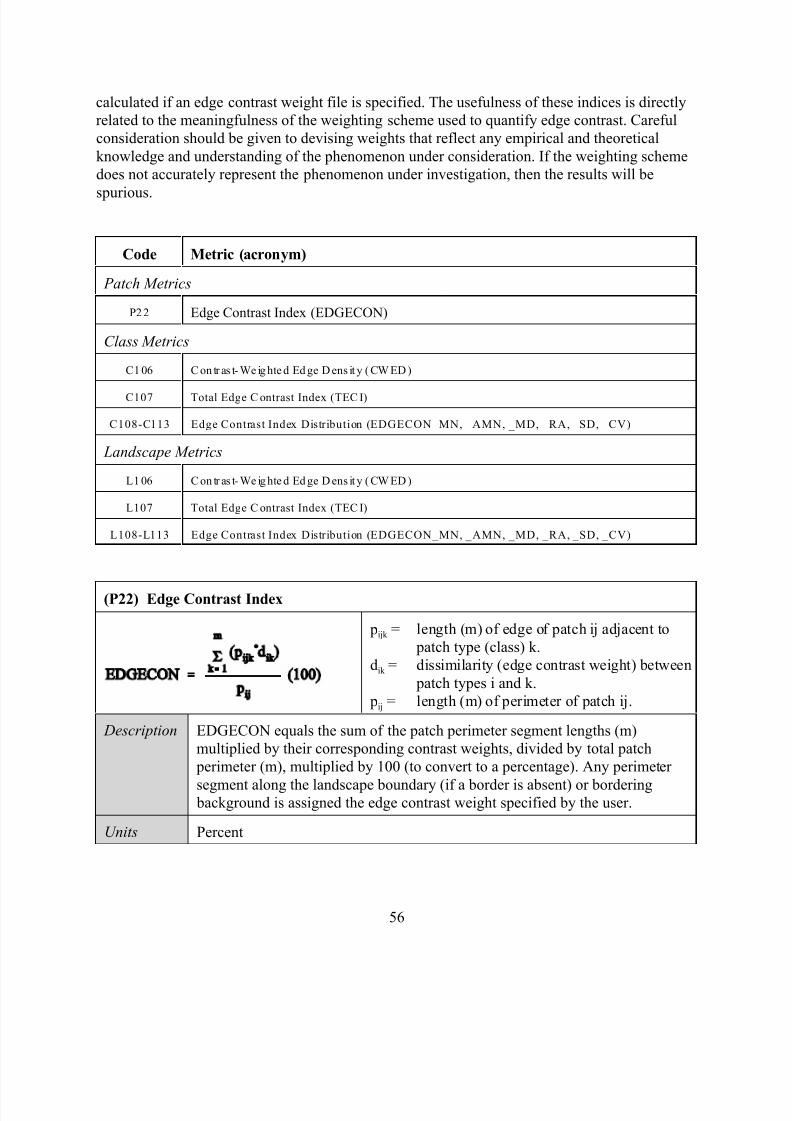
7/14/2019 Bothanical_Metrics
http://slidepdf.com/reader/full/bothanicalmetrics 56/99
56
calculated if an edge contrast weight file is specified. The usefulness of these indices is directly
related to the meaningfulness of the weighting scheme used to quantify edge contrast. Careful
consideration should be given to devising weights that reflect any empirical and theoretical
knowledge and understanding of the phenomenon under consideration. If the weighting scheme
does not accurately represent the phenomenon under investigation, then the results will be
spurious.
Code Metric (acronym)
Patch Metrics
P22 Edge Contrast Index (EDGECON)
Class Metrics
C1 06 C on tr as t- We ig hte d Ed ge D ens it y ( CW ED )
C107 Total Edge C ontrast Index (TEC I)
C108-C113 Edge Contrast Index Distribution (EDGECON_MN, _AMN, _MD, _RA, _SD, _CV)
Landscape Metrics
L1 06 C on tr as t- We ig hte d Ed ge D ens it y ( CW ED )
L107 Total Edge C ontrast Index (TEC I)
L108-L113 Edge Contrast Index Distribution (EDGECON_MN, _AMN, _MD, _RA, _SD, _CV)
(P22) Edge Contrast Index
pijk = length (m) of edge of patch ij adjacent to
patch type (class) k.
dik = dissimilarity (edge contrast weight) between
patch types i and k.
pij = length (m) of perimeter of patch ij.
Description EDGECON equals the sum of the patch perimeter segment lengths (m)
multiplied by their corresponding contrast weights, divided by total patch
perimeter (m), multiplied by 100 (to convert to a percentage). Any perimeter
segment along the landscape boundary (if a border is absent) or bordering background is assigned the edge contrast weight specified by the user.
Units Percent
7/14/2019 Bothanical_Metrics
http://slidepdf.com/reader/full/bothanicalmetrics 57/99
57
Range 0 # EDGECON # 100
EDGECON = 0 if the landscape consists of only 1 patch and either the
landscape boundary contains no edge (when a border is present) or the
boundary is not to be treated as edge (when a border is absent). Also,
EDGECON = 0 when all of the patch perimeter segments involve patch typeadjacencies that have been given a zero-contrast weight (d = 0) in the edge
contrast weight file. EDGECON = 100 when the entire patch perimeter is
maximum-contrast edge (d = 1). EDGECON < 100 when a portion of the patch
perimeter is less than maximum-contrast edge (d < 1).
Comments Edge Contrast Index is founded on the notion that all edges are not created
equal. To account for this, the notion of edge “contrast” was created. This index
is a relative measure of the amount of contrast along the patch perimeter.
(C106) Contrast-Weighted Edge Density
eik = total length (m) of edge in landscape between
patch types (classes) i and k; includes landscape
boundary segments involving patch type i.
dik = dissimilarity (edge contrast weight) between
patch types i and k.
A = total landscape area (m2).
Description CWED equals the sum of the lengths (m) of each edge segment involving the
corresponding patch type multiplied by the corresponding contrast weight,
divided by the total landscape area (m2), multiplied by 10,000 (to convert to
hectares).
Units Meters per hectare
Range CWED $ 0, without limit.
CWED = 0 when there is no class edge in the landscape; that is, when the entire
landscape and landscape border, if present, consists of the corresponding patch
type and the user specifies that none of the landscape boundary and background
edge be treated as edge. CWED increases as the amount of class edge in the
landscape increases and/or as the contrast in edges involving the corresponding
patch type increase (i.e., contrast weight approaches 1).
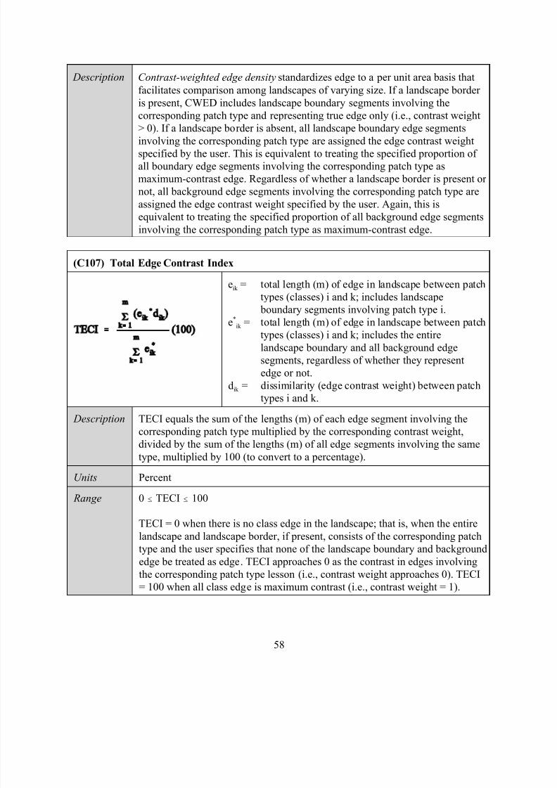
7/14/2019 Bothanical_Metrics
http://slidepdf.com/reader/full/bothanicalmetrics 58/99
58
Description Contrast-weighted edge density standardizes edge to a per unit area basis that
facilitates comparison among landscapes of varying size. If a landscape border
is present, CWED includes landscape boundary segments involving the
corresponding patch type and representing true edge only (i.e., contrast weight
> 0). If a landscape border is absent, all landscape boundary edge segments
involving the corresponding patch type are assigned the edge contrast weightspecified by the user. This is equivalent to treating the specified proportion of
all boundary edge segments involving the corresponding patch type as
maximum-contrast edge. Regardless of whether a landscape border is present or
not, all background edge segments involving the corresponding patch type are
assigned the edge contrast weight specified by the user. Again, this is
equivalent to treating the specified proportion of all background edge segments
involving the corresponding patch type as maximum-contrast edge.
(C107) Total Edge Contrast Index
eik = total length (m) of edge in landscape between patch
types (classes) i and k; includes landscape
boundary segments involving patch type i.
e*ik = total length (m) of edge in landscape between patch
types (classes) i and k; includes the entire
landscape boundary and all background edge
segments, regardless of whether they represent
edge or not.
dik = dissimilarity (edge contrast weight) between patch
types i and k.
Description TECI equals the sum of the lengths (m) of each edge segment involving the
corresponding patch type multiplied by the corresponding contrast weight,
divided by the sum of the lengths (m) of all edge segments involving the same
type, multiplied by 100 (to convert to a percentage).
Units Percent
Range 0 # TECI # 100
TECI = 0 when there is no class edge in the landscape; that is, when the entire
landscape and landscape border, if present, consists of the corresponding patch
type and the user specifies that none of the landscape boundary and backgroundedge be treated as edge. TECI approaches 0 as the contrast in edges involving
the corresponding patch type lesson (i.e., contrast weight approaches 0). TECI
= 100 when all class edge is maximum contrast (i.e., contrast weight = 1).
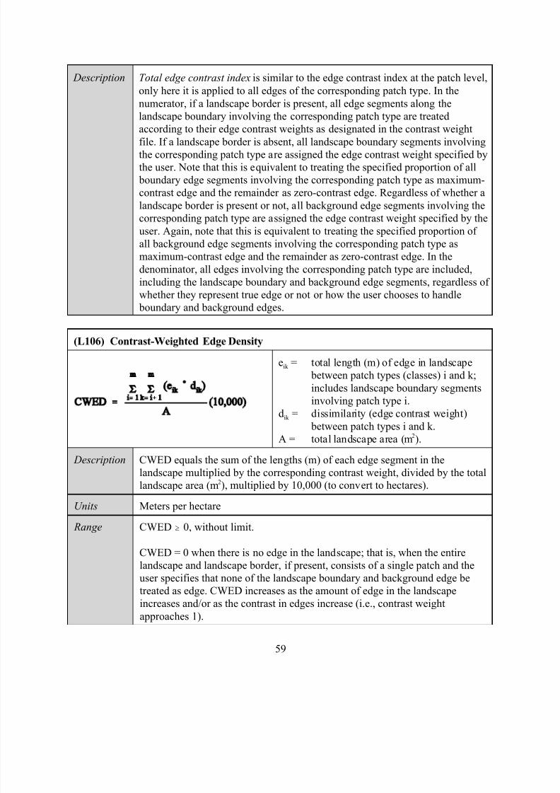
7/14/2019 Bothanical_Metrics
http://slidepdf.com/reader/full/bothanicalmetrics 59/99
59
Description Total edge contrast index is similar to the edge contrast index at the patch level,
only here it is applied to all edges of the corresponding patch type. In the
numerator, if a landscape border is present, all edge segments along the
landscape boundary involving the corresponding patch type are treated
according to their edge contrast weights as designated in the contrast weight
file. If a landscape border is absent, all landscape boundary segments involvingthe corresponding patch type are assigned the edge contrast weight specified by
the user. Note that this is equivalent to treating the specified proportion of all
boundary edge segments involving the corresponding patch type as maximum-
contrast edge and the remainder as zero-contrast edge. Regardless of whether a
landscape border is present or not, all background edge segments involving the
corresponding patch type are assigned the edge contrast weight specified by the
user. Again, note that this is equivalent to treating the specified proportion of
all background edge segments involving the corresponding patch type as
maximum-contrast edge and the remainder as zero-contrast edge. In the
denominator, all edges involving the corresponding patch type are included,
including the landscape boundary and background edge segments, regardless of
whether they represent true edge or not or how the user chooses to handle
boundary and background edges.
(L106) Contrast-Weighted Edge Density
eik = total length (m) of edge in landscape
between patch types (classes) i and k;
includes landscape boundary segments
involving patch type i.
dik = dissimilarity (edge contrast weight) between patch types i and k.
A = total landscape area (m2).
Description CWED equals the sum of the lengths (m) of each edge segment in the
landscape multiplied by the corresponding contrast weight, divided by the total
landscape area (m2), multiplied by 10,000 (to convert to hectares).
Units Meters per hectare
Range CWED $ 0, without limit.
CWED = 0 when there is no edge in the landscape; that is, when the entirelandscape and landscape border, if present, consists of a single patch and the
user specifies that none of the landscape boundary and background edge be
treated as edge. CWED increases as the amount of edge in the landscape
increases and/or as the contrast in edges increase (i.e., contrast weight
approaches 1).
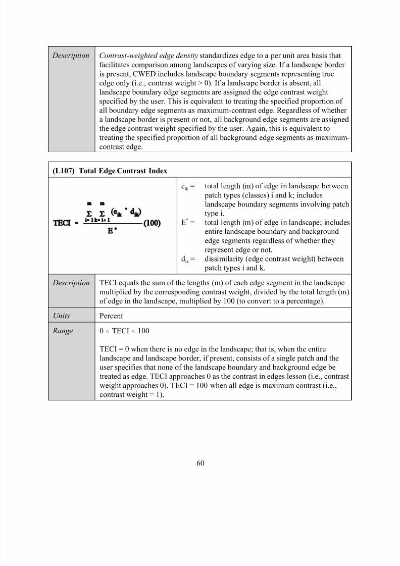
7/14/2019 Bothanical_Metrics
http://slidepdf.com/reader/full/bothanicalmetrics 60/99
60
Description Contrast-weighted edge density standardizes edge to a per unit area basis that
facilitates comparison among landscapes of varying size. If a landscape border
is present, CWED includes landscape boundary segments representing true
edge only (i.e., contrast weight > 0). If a landscape border is absent, all
landscape boundary edge segments are assigned the edge contrast weight
specified by the user. This is equivalent to treating the specified proportion of all boundary edge segments as maximum-contrast edge. Regardless of whether
a landscape border is present or not, all background edge segments are assigned
the edge contrast weight specified by the user. Again, this is equivalent to
treating the specified proportion of all background edge segments as maximum-
contrast edge.
(L107) Total Edge Contrast Index
eik = total length (m) of edge in landscape between
patch types (classes) i and k; includeslandscape boundary segments involving patch
type i.
E* = total length (m) of edge in landscape; includes
entire landscape boundary and background
edge segments regardless of whether they
represent edge or not.
dik = dissimilarity (edge contrast weight) between
patch types i and k.
Description TECI equals the sum of the lengths (m) of each edge segment in the landscape
multiplied by the corresponding contrast weight, divided by the total length (m)
of edge in the landscape, multiplied by 100 (to convert to a percentage).
Units Percent
Range 0 # TECI # 100
TECI = 0 when there is no edge in the landscape; that is, when the entire
landscape and landscape border, if present, consists of a single patch and the
user specifies that none of the landscape boundary and background edge be
treated as edge. TECI approaches 0 as the contrast in edges lesson (i.e., contrast
weight approaches 0). TECI = 100 when all edge is maximum contrast (i.e.,
contrast weight = 1).
7/14/2019 Bothanical_Metrics
http://slidepdf.com/reader/full/bothanicalmetrics 61/99
61
Description Total edge contrast index is similar to the edge contrast index at the patch level,
only here it is applied to all edges across the landscape. In the numerator, if a
landscape border is present, all edge segments along the landscape boundary
are treated according to their edge contrast weights as designated in the contrast
weight file. If a landscape border is absent, all landscape boundary segments
are assigned the edge contrast weight specified by the user. Note that this isequivalent to treating the specified proportion of the landscape boundary as
maximum-contrast edge and the remainder as zero-contrast edge. Regardless of
whether a landscape border is present or not, all background edge segments are
assigned the edge contrast weight specified by the user. Again, note that this is
equivalent to treating the specified proportion of all background edge as
maximum-contrast edge and the remainder as zero-contrast edge. In the
denominator, all edges are included, including the landscape boundary and
background edge segments, regardless of whether they represent true edge or
not or how the user chooses to handle boundary and background edges.
CONTAGION/INTERSPERSION METRICS
Background.--Contagion refers to the tendency of patch types to be spatially aggregated; that is,
to occur in large, aggregated or “contagious” distributions. Contagion ignores patches per se and
measures the extent to which cells of similar class are aggregated. Interspersion, on the other
hand, refers to the intermixing of patches of different types and is based soley on patch (as
opposed to cell) adjacencies. Contagion and interspersion are both aspects of landscape texture;
they both quantify the adjacency of similar patch types, but do so in a different manner. The
texture of a landscape is important in many ecological processes. Contagion, for example, is a
crucial aspect of habitat fragmentation. Specifically, habitat fragmentation involves thesubdivision of contiguous habitat into disjunct patches, which affects the overall spatial
distribution or configuration (i.e., contagion) of habitat within the landscape. As habitat
fragmentation proceeds, habitat contagion decreases and, eventually, ecological function is
impaired (Saunders et al.1991). Similarly, interspersion is presumed to affect the quality of
habitat for many species that require different patch types to meet different life history requisites,
as in the process of landscape complementation (Dunning et al. 1992). Indeed, the notion of
habitat interspersion has had a preeminent role in wildlife management during the past century.
Wildlife management efforts are often focused on maximizing habitat interspersion because it is
believed that the juxtaposition of different habitats will increase species diversity (Leopold
1933).
FRAGSTATS Metrics.–There are several different approaches for measuring contagion and
interspersion. One popular index that subsumes both dispersion and interspersion is the
contagion index (CONTAG) based on the probability of finding a cell of type i next to a cell of
type j. This index was proposed first by O'Neill et al. (1988) and subsequently it has been widely
used (Turner and Ruscher 1988, Turner 1989, Turner et al. 1989, Turner 1990a and b, Graham et
7/14/2019 Bothanical_Metrics
http://slidepdf.com/reader/full/bothanicalmetrics 62/99
62
al. 1991, Gustafson and Parker 1992). Li and Reynolds (1993) showed that the original formula
was incorrect; they introduced 2 forms of an alternative contagion index that corrects this error
and has improved performance. FRAGSTATS computes one of the contagion indices proposed
by Li and Reynolds (1993). This contagion index is based on raster "cell" adjacencies, not
"patch" adjacencies, and consists of the sum, over patch types, of the product of 2 probabilities:
(1) the probability that a randomly chosen cell belongs to patch type i (estimated by the proportional abundance of patch type i), and (2) the conditional probability that given a cell is of
patch type i, one of its neighboring cells belongs to patch type j (estimated by the proportional
abundance of patch type i adjacencies involving patch type j). The product of these probabilities
equals the probability that 2 randomly chosen adjacent cells belong to patch type i and j. This
contagion index is appealing because of the straightforward and intuitive interpretation of this
probability.
The contagion index has been widely used in landscape ecology because it seems to be an
effective summary of overall clumpiness on categorical maps (Turner 1989). In addition, in
many landscapes, it is highly correlated with indices of patch type diversity and dominance
(Ritters et al. 1995) and thus may be an effective surrogate for those important components of pattern (O’Neill et al. 1996). Contagion measures both patch type interspersion (i.e., the
intermixing of units of different patch types) as well as patch dispersion (i.e., the spatial
distribution of a patch type). All other things being equal, a landscape in which the patch types
are well interspersed will have lower contagion than a landscape in which patch types are poorly
interspersed. Contagion measures the extent to which patch types are aggregated or clumped (i.e.,
dispersion); higher values of contagion may result from landscapes with a few large, contiguous
patches, whereas lower values generally characterize landscapes with many small and dispersed
patches. Thus, holding interspersion constant, a landscape in which the patch types are
aggregated into larger, contiguous patches will have greater contagion than a landscape in which
the patch types are fragmented into many small patches. Contagion measures dispersion in
addition to patch type interspersion because cells, not patches, are evaluated for adjacency.Landscapes consisting of large, contiguous patches have a majority of internal cells with like
adjacencies. In this case, contagion is high because the proportion of total cell adjacencies
comprised of like adjacencies is very large and the distribution of adjacencies among edge types
is very uneven.
Unfortunately, as alluded to above, there are alternative procedures for computing contagion, and
this has contributed to some confusion over the interpretation of published contagion values (see
Ritters et al. 1996 for a discussion). Briefly, to calculate contagion, the adjacency of patch types
is first summarized in an “adjacency” or “co-occurrence” matrix, which shows the frequency
with which different pairs of patch types (including like adjacencies between the same patch
type) appear side-by-side on the map. Although this would seem to be a simple task, it is thesource of differences among procedures for calculating contagion. The difference arises out of
the option to count each immediately-adjacent pixel pair once or twice. In the single-count
method, each pixel adjacency is counted once and the order of pixels is not preserved; whereas,
in the double-count method, each pixel adjacency is counted twice and the order of pixels is
preserved. Ritters et al. (1996) discuss the merits of both approaches. FRAGSTATS adopts the
7/14/2019 Bothanical_Metrics
http://slidepdf.com/reader/full/bothanicalmetrics 63/99
63
double-count method in which pixel order is preserved.
McGarigal and Marks (1995) suggest a complementary interspersion and juxtaposition index
(IJI) that increases in value as patches tend to be more evenly interspersed in a "salt and pepper"
mixture. Unlike the earlier contagion indices that are based on raster "cell" adjacencies, this
index is based on "patch" adjacencies; only the patch perimeters are considered in determiningthe total length of each unique edge type. Each patch is evaluated for adjacency with all other
patch types; like adjacencies are not possible because a patch can never be adjacent to a patch of
the same type. Because this index is a measure of "patch" adjacency and not "cell" adjacency, the
interpretation is somewhat different than the contagion index. The interspersion index measures
the extent to which patch types are interspersed (not necessarily dispersed); higher values result
from landscapes in which the patch types are well interspersed (i.e., equally adjacent to each
other), whereas lower values characterize landscapes in which the patch types are poorly
interspersed (i.e., disproportionate distribution of patch type adjacencies). The interspersion
index is not directly affected by the number, size, contiguity, or dispersion of patches per se, as is
the contagion index. Consequently, a landscape containing 4 large patches, each a different patch
type, and a landscape of the same extent containing 100 small patches of 4 patch types will havethe same index value if the patch types are equally interspersed (or adjacent to each other based
on the proportion of total edge length in each edge type); whereas, the value of contagion would
be quite different. Like the contagion index, the interspersion index is a relative index that
represents the observed level of interspersion as a percentage of the maximum possible given the
total number of patch types.
It is important to note the differences between the contagion index and the interspersion and
juxtaposition index. Contagion is affected by both interspersion and dispersion. The interspersion
and juxtaposition index, in contrast, is affected only by patch type interspersion and juxtaposition
and not necessarily by the size, contiguity, or dispersion of patches. Thus, although often
indirectly affected by dispersion, the interspersion and juxtaposition index directly measures patch type interspersion, whereas contagion measures a combination of both patch type
interspersion and dispersion. In addition, contagion and interspersion are typically inversely
related to each other. Higher contagion generally corresponds to lower interspersion and vice
versa. Finally, in contrast to the interspersion and juxtaposition index, the contagion index is
strongly affected by the grain size or resolution of the image. Given a particular patch mosaic, a
smaller grain size will result in greater contagion because of the proportional increase in like
adjacencies from internal cells. The interspersion and juxtaposition index is not affected in this
manner because it considers only patch edges. This scale effect should be carefully considered
when attempting to compare results from different studies.
Other contagion-like metrics can be generated from the matrix of pairwise adjacencies between patch types. FRAGSTATS computes the percentage of like adjacencies (PLADJ), which is
computed as the sum of the diagonal elements (i.e., like adjacencies) of the adjacency matrix
divided by the total number of adjacencies. A landscape containing greater aggregation of patch
types (e.g., larger patches with compact shapes) will contain a higher proportion of like
adjacencies than a landscape containing disaggregated patch types (e.g., smaller patches and
7/14/2019 Bothanical_Metrics
http://slidepdf.com/reader/full/bothanicalmetrics 64/99
64
more complex shapes). In contrast to the contagion index, this metric measures only patch type
dispersion, not interspersion, and is unaffected by the method used to summarize adjacencies. At
the class level, this metric is computed as the percentage of like adjacencies of the focal class. A
highly contagious (aggregated) patch type will contain a higher percentage of like adjacencies.
Conversely, a highly fragmented (disaggregated) patch type will contain proportionately fewer
like adjacencies. As such, this index provides an effective measure of class-specific contagionthat isolates the dispersion (as opposed to interspersion) component of configuration. However,
this index requires careful interpretation because it varies in relation to the proportion of the
landscape comprised of the focal class (Pi). It has been shown that PLADJ for class i will equal Pi
for a completely random map (Gardner and O’Neill 1991). If the focal class is more dispersed
than is expected of a random distribution (i.e., overdispersed), then PLADJ < Pi. If the focal class
is more contagiously distributed, then PLADJ > Pi. Thus, although PLADJ provides an absolute
measure of aggregation of the focal class, it is difficult to interpret as a measure of contagion
without adjusting for Pi. Consequently, FRAGSTATS computes a new class-specific contagion
index based on PLADJ that adjusts for Pi. Specifically, the contagion index at the class level is
computed as a percentage such that it returns a value of 50% for a random distribution, regardless
of Pi, Values less than 50% indicate greater dispersion (or disaggregation) than expected of arandom distribution, and values greater than 50% indicate greater contagion. Hence, this index
provides a measure of class-specific contagion that effectively isolates the configuration
component from the area component and, as such, provides an effective index of fragmentation
of the focal class that is not confounded by changes in class area.
There are alternative methods for calculating class-specific contagion using fractal geometry
(Gardner and O’Neill 1991). FRAGSTATS computes the mass fractal dimension (MFRAC) for
each class, which is based on the scaling relationship between box mass (i.e., the number of
pixels of a focal class within a window) and the size of the box defining the window (r).
Specifically, a range of box sizes is used to delineate windows, from 3 pixels on a side (r=3) to a
maximum of approximatelya of the landscape. For each box size, the mean number of pixels of the focal class is determined by centering the box on every pixel of that class and counting the
number of pixels of that class in the box sample. Mass fractal dimension is equal to the slope
derived from regressing the log of the mean number of pixels for each box size on the log of the
box lengths (Voss 1988, Milne 1991). Mass fractal dimension decreases as the percentage of the
landscape comprised of the focal class decreases. After accounting for this relationship, higher
values of mass fractal dimension are associated with higher contagion.
Lacunarity is another method borrowed from fractal geometry by which contagion can be
characterized at the class level across a range of spatial scales (Plotnick et al. 1993 and 1996,
Dale 2000). Consider a binary ("on/off") raster map of dimension m. The technique involves
using a moving window and is concerned with the frequency with which one encounters thefocal class in a window of different sizes, similar to the mass fractal dimension. To do this, a
gliding box is constructed of dimension r, and a frequency distribution of tallies of S=1,2, ..., r 2
"on" cells is constructed. In this gliding, the box is moved over one cell at a time, so that the
boxes overlap during the sliding. Define n(S,r) as the number of boxes that tally S "on" cells for a
box of size r. There are N(r)=(m-r+1)2 boxes of size r, and the probability associated with n(S,r)
7/14/2019 Bothanical_Metrics
http://slidepdf.com/reader/full/bothanicalmetrics 65/99
65
is Q(S,r)=n(S,r)/N(r). The first and second moments of Q are used to define lacunarity L
(lambda) for this box size as a variance to mean-square ratio. This is repeated for a range of box
sizes r. A log-log plot of lacunarity against window size expresses the contagion of the map, or
its tendency to aggregate into discrete patches, across a range of spatial scales. Note that as r
increases, the tally n(S,r) converges on the mean and its variance converges on 0. Thus, for very
large boxes L=1 and ln(L)=0. At the smallest box size (r=1), L(1) = 1/p, where p is the proportion of the map occupied ("on"). Thus, for the finest resolution of a map, L depends solely
on p. At intermediate scales, lacunarity expresses the contagion of the map, or its tendency to
clump into discrete patches. So the lacunarity plot summarizes the contagion of the map across
all scales.
Limitations.–All measures based on the adjacency matrix (i.e., the number of adjacencies
between each pair of patch types)[contagion and proportion of like adjacencies] are strongly
affected by the grain size or resolution of the image. Given a particular patch mosaic, a smaller
grain size will result in a proportional increase in like adjacencies. Given this scale dependency,
these metrics are best used if the scale is held constant. In addition, there are alternative ways to
consider cell adjacencies. Adjacencies may include only the 4 cells sharing a side with the focalcell, or they may include the diagonal neighbors as well. FRAGSTATS uses the 4-neighbor
approach for the purpose of calculating these metrics. Finally, mass fractal dimension and
lacunarity involve the use of moving windows of many sizes; these can be computationally
demanding and for large landscapes may take a very long time to compute.
Metrics based on fractal geometry such as mass fractal dimension are subject to several
limitations (as discussed by Hargis et al. 1998). First, the simplifications of landscape pattern
produced during the mapping process yield images that are not truly fractal, and the application
of fractal measures in the strictest sense is therefore questionable. Fractal geometry assumes that
the quantity being measured and the ruler length of measurement have a linear relationship when
both are logarithmically transformed (Voss 1988). If this condition is not met, the object (in thiscase, the landscape) may not be fractal. Any smoothing or renormalization of landscape patterns
during the mapping process may cause this relationship to deviate from linearity, and the use of
fractal dimension may be questionable. Second, landscape extent and grain affect the ability to
derive an accurate scaling relationship between box size and mass. A large ratio of extent to grain
is needed to produce a reasonable range of box sizes for generating an accurate slope. Finally, the
relationship between grain and average patch size can affect the accuracy and meaningfulness of
the derived fractal dimension. If map resolution allows only two or three box sizes before the
sample box exceeds the size of the average patch, the slope derived from these points is
questionable. In this case, when larger box sizes are added to the regression line, any interesting
differences are lost in the averaging process.
Code Metric (acronym)
Class Metrics
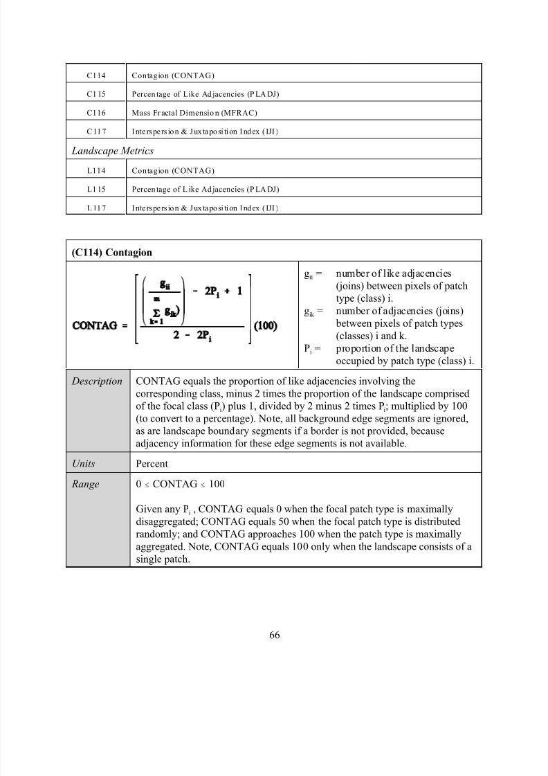
7/14/2019 Bothanical_Metrics
http://slidepdf.com/reader/full/bothanicalmetrics 66/99
66
C114 Contagion (CONTAG)
C1 15 Percen tage of Like Ad jacencies (P LA DJ)
C116 Mass Fr actal Dimensio n (MFRAC)
C 117 Inte rspe rs ion & Juxtaposi ti on Index ( IJI )
Landscape Metrics
L114 Contagion (CONTAG)
L1 15 Percen tage of L ike Ad jacencies (P LA DJ)
L117 Inte rspe rs ion & Juxtaposi ti on Index ( IJI )
(C114) Contagion
gii = number of like adjacencies(joins) between pixels of patch
type (class) i.
gik = number of adjacencies (joins)
between pixels of patch types
(classes) i and k.
Pi = proportion of the landscape
occupied by patch type (class) i.
Description CONTAG equals the proportion of like adjacencies involving the
corresponding class, minus 2 times the proportion of the landscape comprised
of the focal class (Pi) plus 1, divided by 2 minus 2 times Pi; multiplied by 100(to convert to a percentage). Note, all background edge segments are ignored,
as are landscape boundary segments if a border is not provided, because
adjacency information for these edge segments is not available.
Units Percent
Range 0 # CONTAG # 100
Given any Pi , CONTAG equals 0 when the focal patch type is maximally
disaggregated; CONTAG equals 50 when the focal patch type is distributed
randomly; and CONTAG approaches 100 when the patch type is maximally
aggregated. Note, CONTAG equals 100 only when the landscape consists of asingle patch.
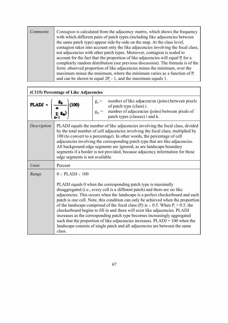
7/14/2019 Bothanical_Metrics
http://slidepdf.com/reader/full/bothanicalmetrics 67/99
67
Comments Contagion is calculated from the adjacency matrix, which shows the frequency
with which different pairs of patch types (including like adjacencies between
the same patch type) appear side-by-side on the map. At the class level,
contagion takes into account only the like adjacencies involving the focal class,
not adjacencies with other patch types. Moreover, contagion is scaled to
account for the fact that the proportion of like adjacencies will equal Pi for acompletely random distribution (see previous discussion). The formula is of the
form: observed proportion of like adjacencies minus the minimum, over the
maximum minus the minimum, where the minimum varies as a function of Pi
and can be shown to equal 2Pi - 1, and the maximum equals 1.
(C115) Percentage of Like Adjacencies
gii = number of like adjacencies (joins) between pixels
of patch type (class) i.
gik = number of adjacencies (joins) between pixels of patch types (classes) i and k.
Description PLADJ equals the number of like adjacencies involving the focal class, divided
by the total number of cell adjacencies involving the focal class; multiplied by
100 (to convert to a percentage). In other words, the percentage of cell
adjacencies involving the corresponding patch type that are like adjacencies.
All background edge segments are ignored, as are landscape boundary
segments if a border is not provided, because adjacency information for these
edge segments is not available.
Units Percent
Range 0 # PLADJ # 100
PLADJ equals 0 when the corresponding patch type is maximally
disaggregated (i.e., every cell is a different patch) and there are no like
adjacencies. This occurs when the landscape is a perfect checkerboard and each
patch is one cell. Note, this condition can only be achieved when the proportion
of the landscape comprised of the focal class (Pi) is # 0.5. When Pi > 0.5, the
checkerboard begins to fill in and there will exist like adjacencies. PLADJ
increases as the corresponding patch type becomes increasingly aggregated
such that the proportion of like adjacencies increases. PLADJ = 100 when the
landscape consists of single patch and all adjacencies are between the sameclass.
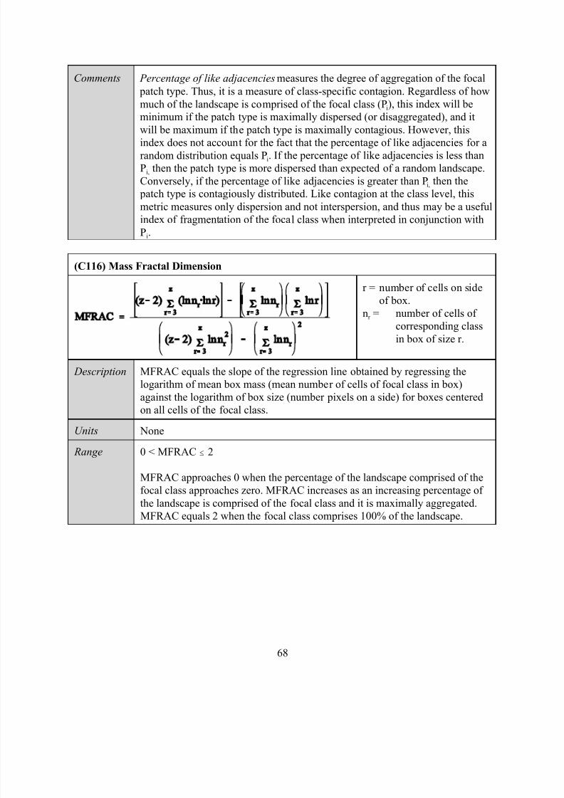
7/14/2019 Bothanical_Metrics
http://slidepdf.com/reader/full/bothanicalmetrics 68/99
68
Comments Percentage of like adjacencies measures the degree of aggregation of the focal
patch type. Thus, it is a measure of class-specific contagion. Regardless of how
much of the landscape is comprised of the focal class (Pi), this index will be
minimum if the patch type is maximally dispersed (or disaggregated), and it
will be maximum if the patch type is maximally contagious. However, this
index does not account for the fact that the percentage of like adjacencies for arandom distribution equals Pi. If the percentage of like adjacencies is less than
Pi, then the patch type is more dispersed than expected of a random landscape.
Conversely, if the percentage of like adjacencies is greater than Pi, then the
patch type is contagiously distributed. Like contagion at the class level, this
metric measures only dispersion and not interspersion, and thus may be a useful
index of fragmentation of the focal class when interpreted in conjunction with
Pi.
(C116) Mass Fractal Dimension
r = number of cells on side
of box.
nr = number of cells of
corresponding class
in box of size r.
Description MFRAC equals the slope of the regression line obtained by regressing the
logarithm of mean box mass (mean number of cells of focal class in box)
against the logarithm of box size (number pixels on a side) for boxes centered
on all cells of the focal class.
Units None
Range 0 < MFRAC # 2
MFRAC approaches 0 when the percentage of the landscape comprised of the
focal class approaches zero. MFRAC increases as an increasing percentage of
the landscape is comprised of the focal class and it is maximally aggregated.
MFRAC equals 2 when the focal class comprises 100% of the landscape.
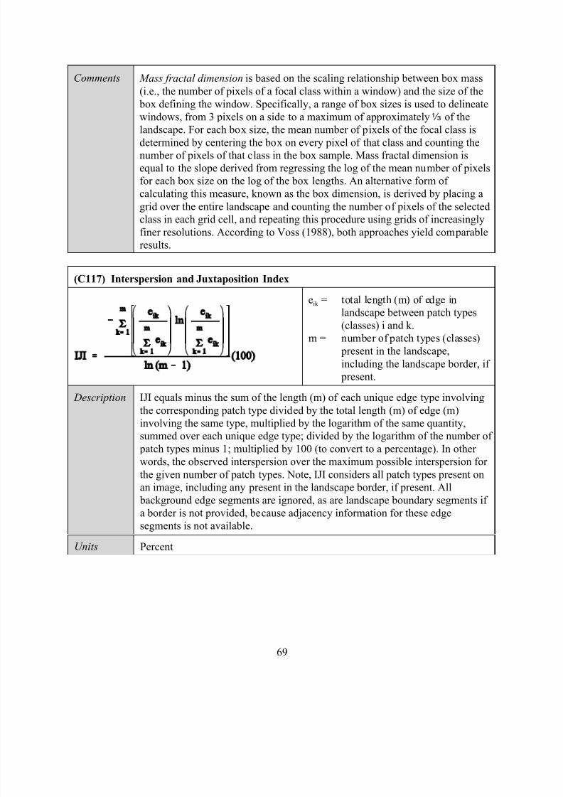
7/14/2019 Bothanical_Metrics
http://slidepdf.com/reader/full/bothanicalmetrics 69/99
69
Comments Mass fractal dimension is based on the scaling relationship between box mass
(i.e., the number of pixels of a focal class within a window) and the size of the
box defining the window. Specifically, a range of box sizes is used to delineate
windows, from 3 pixels on a side to a maximum of approximately a of the
landscape. For each box size, the mean number of pixels of the focal class is
determined by centering the box on every pixel of that class and counting thenumber of pixels of that class in the box sample. Mass fractal dimension is
equal to the slope derived from regressing the log of the mean number of pixels
for each box size on the log of the box lengths. An alternative form of
calculating this measure, known as the box dimension, is derived by placing a
grid over the entire landscape and counting the number of pixels of the selected
class in each grid cell, and repeating this procedure using grids of increasingly
finer resolutions. According to Voss (1988), both approaches yield comparable
results.
(C117) Interspersion and Juxtaposition Index
eik = total length (m) of edge in
landscape between patch types
(classes) i and k.
m = number of patch types (classes)
present in the landscape,
including the landscape border, if
present.
Description IJI equals minus the sum of the length (m) of each unique edge type involving
the corresponding patch type divided by the total length (m) of edge (m)
involving the same type, multiplied by the logarithm of the same quantity,
summed over each unique edge type; divided by the logarithm of the number of
patch types minus 1; multiplied by 100 (to convert to a percentage). In other
words, the observed interspersion over the maximum possible interspersion for
the given number of patch types. Note, IJI considers all patch types present on
an image, including any present in the landscape border, if present. All
background edge segments are ignored, as are landscape boundary segments if
a border is not provided, because adjacency information for these edge
segments is not available.
Units Percent
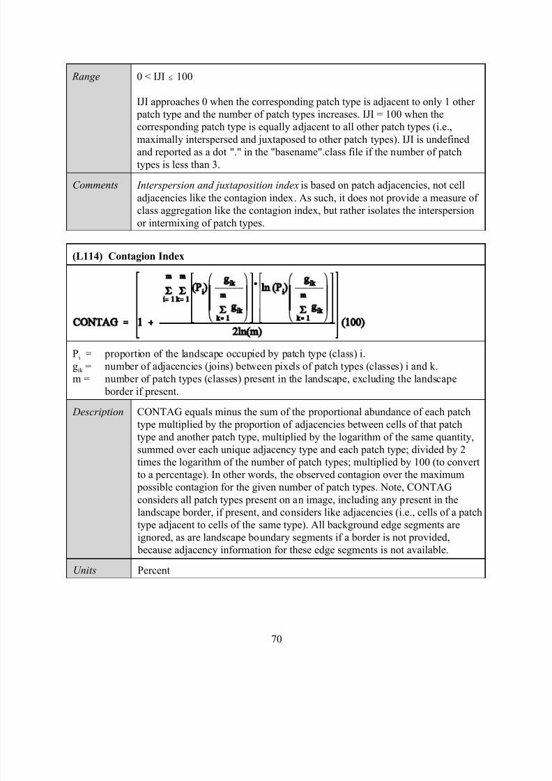
7/14/2019 Bothanical_Metrics
http://slidepdf.com/reader/full/bothanicalmetrics 70/99
70
Range 0 < IJI # 100
IJI approaches 0 when the corresponding patch type is adjacent to only 1 other
patch type and the number of patch types increases. IJI = 100 when the
corresponding patch type is equally adjacent to all other patch types (i.e.,
maximally interspersed and juxtaposed to other patch types). IJI is undefinedand reported as a dot "." in the "basename".class file if the number of patch
types is less than 3.
Comments Interspersion and juxtaposition index is based on patch adjacencies, not cell
adjacencies like the contagion index. As such, it does not provide a measure of
class aggregation like the contagion index, but rather isolates the interspersion
or intermixing of patch types.
(L114) Contagion Index
Pi = proportion of the landscape occupied by patch type (class) i.
gik = number of adjacencies (joins) between pixels of patch types (classes) i and k.
m = number of patch types (classes) present in the landscape, excluding the landscape
border if present.
Description CONTAG equals minus the sum of the proportional abundance of each patchtype multiplied by the proportion of adjacencies between cells of that patch
type and another patch type, multiplied by the logarithm of the same quantity,
summed over each unique adjacency type and each patch type; divided by 2
times the logarithm of the number of patch types; multiplied by 100 (to convert
to a percentage). In other words, the observed contagion over the maximum
possible contagion for the given number of patch types. Note, CONTAG
considers all patch types present on an image, including any present in the
landscape border, if present, and considers like adjacencies (i.e., cells of a patch
type adjacent to cells of the same type). All background edge segments are
ignored, as are landscape boundary segments if a border is not provided,
because adjacency information for these edge segments is not available.
Units Percent
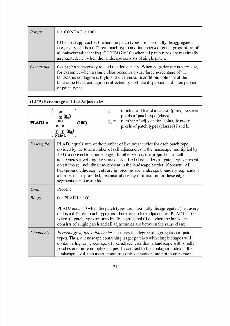
7/14/2019 Bothanical_Metrics
http://slidepdf.com/reader/full/bothanicalmetrics 71/99
71
Range 0 < CONTAG # 100
CONTAG approaches 0 when the patch types are maximally disaggregated
(i.e., every cell is a different patch type) and interspersed (equal proportions of
all pairwise adjacencies). CONTAG = 100 when all patch types are maximally
aggregated; i.e., when the landscape consists of single patch.
Comments Contagion is inversely related to edge density. When edge density is very low,
for example, when a single class occupies a very large percentage of the
landscape, contagion is high, and vice versa. In addition, note that at the
landscape level, contagion is affected by both the dispersion and interspersion
of patch types.
(L115) Percentage of Like Adjacencies
gii = number of like adjacencies (joins) between
pixels of patch type (class) i.gik = number of adjacencies (joins) between
pixels of patch types (classes) i and k.
Description PLADJ equals sum of the number of like adjacencies for each patch type,
divided by the total number of cell adjacencies in the landscape; multiplied by
100 (to convert to a percentage). In other words, the proportion of cell
adjacencies involving the same class. PLADJ considers all patch types present
on an image, including any present in the landscape border, if present. All
background edge segments are ignored, as are landscape boundary segments if a border is not provided, because adjacency information for these edge
segments is not available.
Units Percent
Range 0 # PLADJ # 100
PLADJ equals 0 when the patch types are maximally disaggregated (i.e., every
cell is a different patch type) and there are no like adjacencies. PLADJ = 100
when all patch types are maximally aggregated ( i.e., when the landscape
consists of single patch and all adjacencies are between the same class).
Comments Percentage of like adjacencies measures the degree of aggregation of patch
types. Thus, a landscape containing larger patches with simple shapes will
contain a higher percentage of like adjacencies than a landscape with smaller
patches and more complex shapes. In contrast to the contagion index at the
landscape level, this metric measures only dispersion and not interspersion.
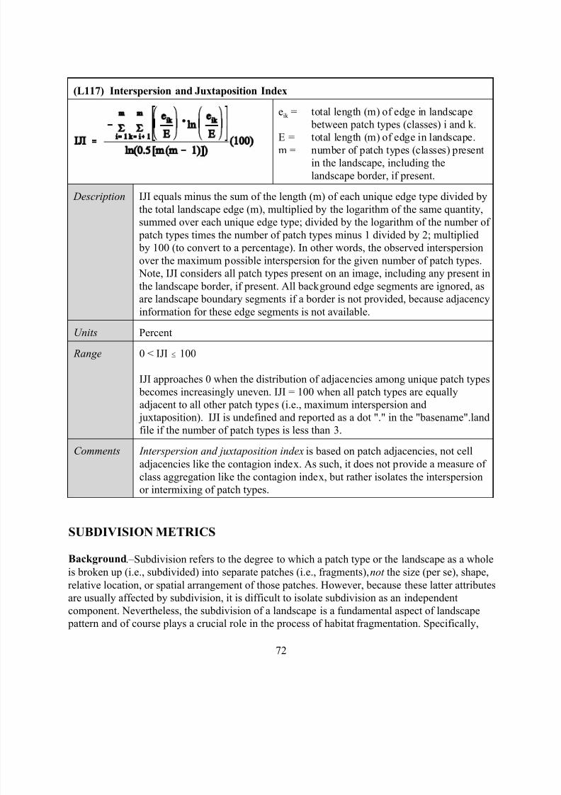
7/14/2019 Bothanical_Metrics
http://slidepdf.com/reader/full/bothanicalmetrics 72/99
72
(L117) Interspersion and Juxtaposition Index
eik = total length (m) of edge in landscape
between patch types (classes) i and k.
E = total length (m) of edge in landscape.m = number of patch types (classes) present
in the landscape, including the
landscape border, if present.
Description IJI equals minus the sum of the length (m) of each unique edge type divided by
the total landscape edge (m), multiplied by the logarithm of the same quantity,
summed over each unique edge type; divided by the logarithm of the number of
patch types times the number of patch types minus 1 divided by 2; multiplied
by 100 (to convert to a percentage). In other words, the observed interspersion
over the maximum possible interspersion for the given number of patch types.
Note, IJI considers all patch types present on an image, including any present inthe landscape border, if present. All background edge segments are ignored, as
are landscape boundary segments if a border is not provided, because adjacency
information for these edge segments is not available.
Units Percent
Range 0 < IJI # 100
IJI approaches 0 when the distribution of adjacencies among unique patch types
becomes increasingly uneven. IJI = 100 when all patch types are equally
adjacent to all other patch types (i.e., maximum interspersion and
juxtaposition). IJI is undefined and reported as a dot "." in the "basename".landfile if the number of patch types is less than 3.
Comments Interspersion and juxtaposition index is based on patch adjacencies, not cell
adjacencies like the contagion index. As such, it does not provide a measure of
class aggregation like the contagion index, but rather isolates the interspersion
or intermixing of patch types.
SUBDIVISION METRICS
Background.–Subdivision refers to the degree to which a patch type or the landscape as a wholeis broken up (i.e., subdivided) into separate patches (i.e., fragments), not the size (per se), shape,
relative location, or spatial arrangement of those patches. However, because these latter attributes
are usually affected by subdivision, it is difficult to isolate subdivision as an independent
component. Nevertheless, the subdivision of a landscape is a fundamental aspect of landscape
pattern and of course plays a crucial role in the process of habitat fragmentation. Specifically,
7/14/2019 Bothanical_Metrics
http://slidepdf.com/reader/full/bothanicalmetrics 73/99
73
habitat fragmentation involves the subdivision of contiguous habitat into disjunct patches, which
affects the overall spatial distribution or configuration (i.e., contagion) of habitat within the
landscape. As habitat fragmentation proceeds, habitat contagion decreases and, eventually,
ecological function is impaired (Saunders et al.1991). Specifically, the subdivision and isolation
of populations caused by this fragmentation can lead to reduced dispersal success and patch
colonization rates which may result in a decline in the persistence of individual populations andan enhanced probability of regional extinction for entire populations across the landscape (e.g.,
Lande 1987; With and King 1999a,b; With 1999). In addition, habitat subdivision may affect the
propagation of disturbances across a landscape (Franklin and Forman 1987). Specifically, a patch
type that is highly subdivided may be more resistant to the propagation of some disturbances
(e.g., disease, fire, etc.), and thus more likely to persist in a landscape than a patch type that is
contiguous. Conversely, habitat fragments may suffer higher rates of disturbance for some
disturbance types (e.g. windthrow) than contiguous habitats.
FRAGSTATS Metrics.–Subdivision can be evaluated using a variety of metrics presented
elsewhere; for example, the number, density, and average size of patches and the degree of
contagion all indirectly relate to subdivision. However, these metrics have been criticized for their insensitivity and inconsistent behavior across a wide of subdivision patterns. Jaeger (2000)
discussed the limitations of these metrics for evaluating habitat fragmentation and concluded that
most of these metrics do not behave in a consistent and logical manner across all phases of the
fragmentation process. He introduced a suite of metrics derived from the cumulative distribution
of patch sizes that provide alternative and more explicit measures of subdivision. When applied
at the class level, these metrics can be used to measure the degree of fragmentation of the focal
patch type. Applied at the landscape level, these metrics measure the graininess of the landscape;
i.e., the tendency of the landscape to exhibit a fine- versus coarse-grain texture. A fine-grain
landscape is characterized by many small patches (highly subdivided); whereas, a coarse-grain
landscape is characterized by fewer large patches.
FRAGSTATS computes three of the subdivision metrics proposed by Jaeger (2000). All of these
metrics are based on the notion that two animals, placed randomly in different areas somewhere
in a region, will have a certain likelihood of being in the same undissected area (i.e., the same
patch) that is a function of the degree of subdivision of the landscape. The landscape division
index (DIVISION) is based on the degree of coherence (C), which is defined as the probability
that two animals placed in different areas somewhere in the region of investigation might find
each other. Degree of coherence is based on the cumulative patch area distribution and is
represented graphically as the area above the cumulative area distribution curve. Degree of
coherence represents the probability that two animals, which have been able to move throughout
the whole region before the landscape was subdivided, will be found in the same patch after the
subdivision is in place. The degree of landscape division is defined as the probability that tworandomly chosen places in the landscape are not situated in the same undissected patch, and is
equal to the complement of the degree of coherence, or the area below the cumulative area
distribution curve.
The splitting index (SPLIT) is defined as the number of patches one gets when dividing the total
7/14/2019 Bothanical_Metrics
http://slidepdf.com/reader/full/bothanicalmetrics 74/99
74
landscape into patches of equal size in such a way that this new configuration leads to the same
degree of landscape division as obtained for the observed cumulative area distribution. Splitting
index can be interpreted to be the “effective mesh number” of a patch mosaic with a constant
patch size dividing the landscape into S patches, where S is the splitting index. The effective
mesh size (MESH) simply denotes the size of the patches when the landscape is divided into S
areas (each of the same size) with the same degree of landscape division as obtained for theobserved cumulative area distribution. Thus, all three subdivision metrics are easily computed
from the cumulative patch area distribution. These measures have the particular advantage over
other conventional measures of subdivision (e.g., mean patch size, patch density) in that they are
insensitive to the omission or addition of very small patches. In practice, this makes the results
more reproducible as investigators do not always use the same lower limit of patch size. Jaeger
(2000) argues that the most important and advantageous feature of these new measures is that
effective mesh size is ‘area-proportionately additive’; that is, it characterizes the subdivision of a
landscape independently of its size.
Limitations.–These metrics are essentially free of any known limitations. Perhaps the greatest
limitation is that they have not yet been used extensively by landscape ecologists, so their behavior under various conditions has not been fully explored. In addition, it is important to keep
in mind the similarities and differences between these metrics and the closely related concept of
contagion. Both contagion and subdivision as defined here refer to the aggregation of patch
types. At the class level, both are exclusively affected by the subdivision of the focal patch type.
However, at the landscape level, contagion is also affected by the interspersion of different patch
types; whereas, these subdivision metrics area not. Moreover, these two groups of metrics are
computed in very different ways. Contagion is computed from the matrix of cell adjacencies,
whereas these subdivision metrics are computed from the cumulative patch area distribution.
Code Metric (acronym)
Class Metrics
C118 L and scap e Divi sion In dex (D IV IS IO N)
C119 Splitting Index (SPLIT)
C120 Effective Mesh Size (MESH)
Landscape Metrics
L118 La nd sc ap e Di vi si on In dex (D IV IS IO N)
L119 Splitting Index (SPLIT)
L120 Effective Mesh Size (MESH)
(C118) Landscape Division Index
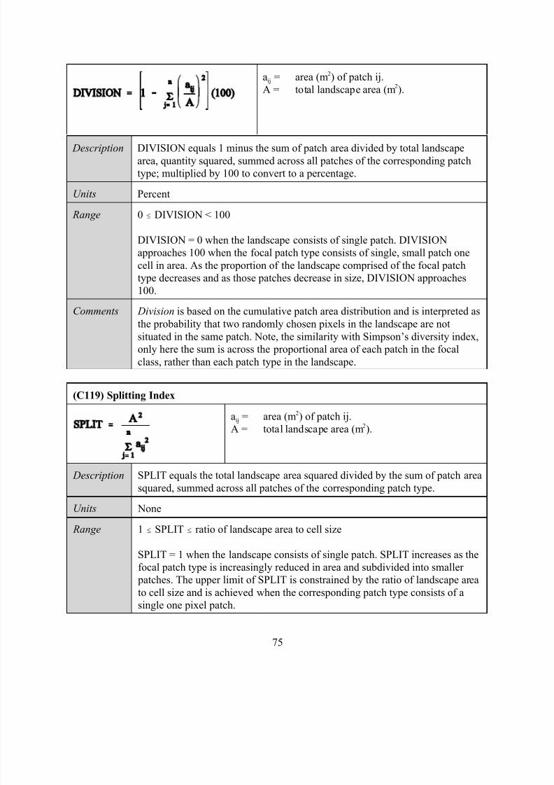
7/14/2019 Bothanical_Metrics
http://slidepdf.com/reader/full/bothanicalmetrics 75/99
75
aij = area (m2) of patch ij.
A = total landscape area (m2).
Description DIVISION equals 1 minus the sum of patch area divided by total landscape
area, quantity squared, summed across all patches of the corresponding patch
type; multiplied by 100 to convert to a percentage.
Units Percent
Range 0 # DIVISION < 100
DIVISION = 0 when the landscape consists of single patch. DIVISION
approaches 100 when the focal patch type consists of single, small patch one
cell in area. As the proportion of the landscape comprised of the focal patch
type decreases and as those patches decrease in size, DIVISION approaches100.
Comments Division is based on the cumulative patch area distribution and is interpreted as
the probability that two randomly chosen pixels in the landscape are not
situated in the same patch. Note, the similarity with Simpson’s diversity index,
only here the sum is across the proportional area of each patch in the focal
class, rather than each patch type in the landscape.
(C119) Splitting Index
aij = area (m2) of patch ij.A = total landscape area (m2).
Description SPLIT equals the total landscape area squared divided by the sum of patch area
squared, summed across all patches of the corresponding patch type.
Units None
Range 1 # SPLIT # ratio of landscape area to cell size
SPLIT = 1 when the landscape consists of single patch. SPLIT increases as the
focal patch type is increasingly reduced in area and subdivided into smaller
patches. The upper limit of SPLIT is constrained by the ratio of landscape area
to cell size and is achieved when the corresponding patch type consists of a
single one pixel patch.
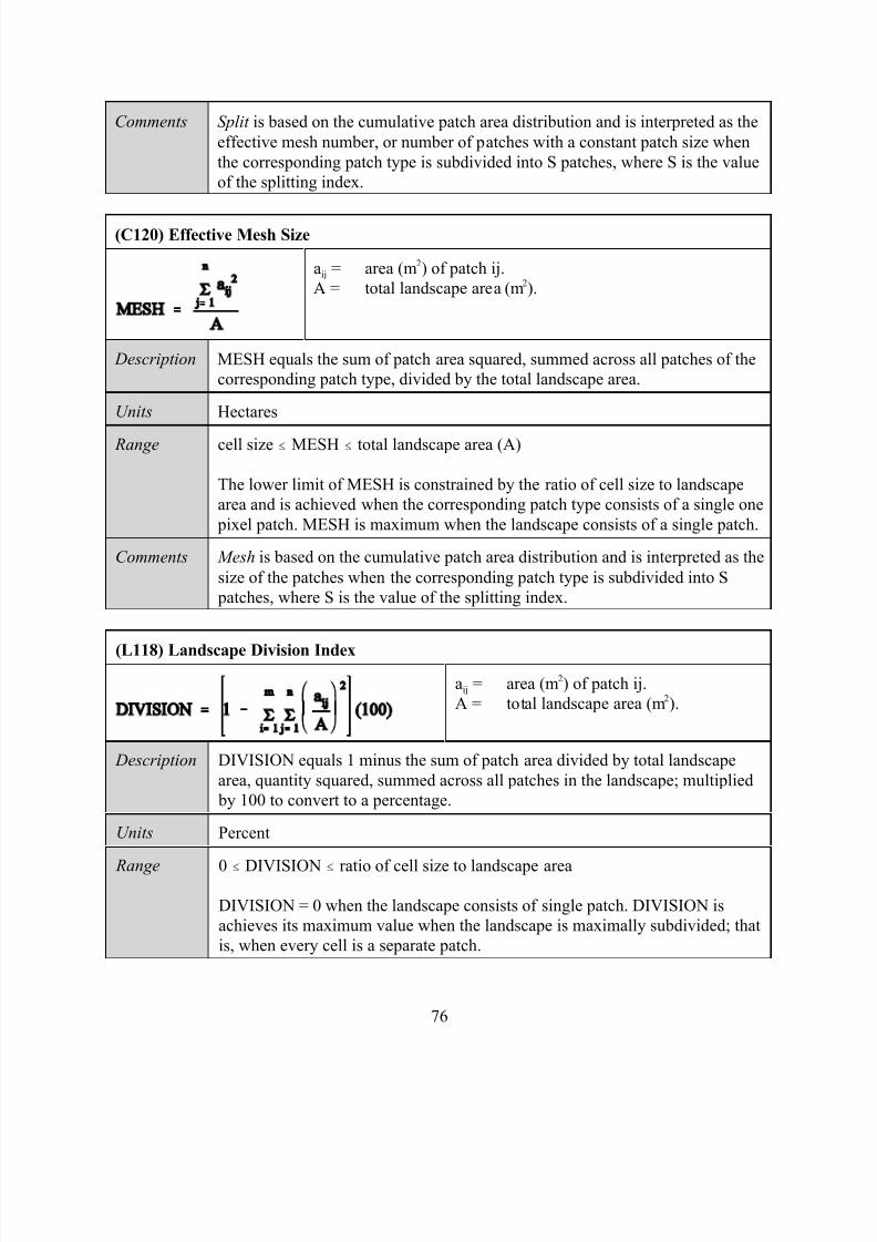
7/14/2019 Bothanical_Metrics
http://slidepdf.com/reader/full/bothanicalmetrics 76/99
76
Comments Split is based on the cumulative patch area distribution and is interpreted as the
effective mesh number, or number of patches with a constant patch size when
the corresponding patch type is subdivided into S patches, where S is the value
of the splitting index.
(C120) Effective Mesh Size
aij = area (m2) of patch ij.
A = total landscape area (m2).
Description MESH equals the sum of patch area squared, summed across all patches of the
corresponding patch type, divided by the total landscape area.
Units Hectares
Range cell size # MESH # total landscape area (A)
The lower limit of MESH is constrained by the ratio of cell size to landscape
area and is achieved when the corresponding patch type consists of a single one
pixel patch. MESH is maximum when the landscape consists of a single patch.
Comments Mesh is based on the cumulative patch area distribution and is interpreted as the
size of the patches when the corresponding patch type is subdivided into S
patches, where S is the value of the splitting index.
(L118) Landscape Division Index
aij = area (m2) of patch ij.
A = total landscape area (m2).
Description DIVISION equals 1 minus the sum of patch area divided by total landscape
area, quantity squared, summed across all patches in the landscape; multiplied
by 100 to convert to a percentage.
Units Percent
Range 0 # DIVISION # ratio of cell size to landscape area
DIVISION = 0 when the landscape consists of single patch. DIVISION is
achieves its maximum value when the landscape is maximally subdivided; that
is, when every cell is a separate patch.
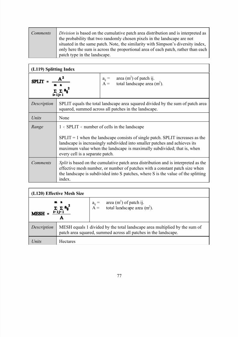
7/14/2019 Bothanical_Metrics
http://slidepdf.com/reader/full/bothanicalmetrics 77/99
77
Comments Division is based on the cumulative patch area distribution and is interpreted as
the probability that two randomly chosen pixels in the landscape are not
situated in the same patch. Note, the similarity with Simpson’s diversity index,
only here the sum is across the proportional area of each patch, rather than each
patch type in the landscape.
(L119) Splitting Index
aij = area (m2) of patch ij.
A = total landscape area (m2).
Description SPLIT equals the total landscape area squared divided by the sum of patch area
squared, summed across all patches in the landscape.
Units None
Range 1 # SPLIT # number of cells in the landscape
SPLIT = 1 when the landscape consists of single patch. SPLIT increases as the
landscape is increasingly subdivided into smaller patches and achieves its
maximum value when the landscape is maximally subdivided; that is, when
every cell is a separate patch.
Comments Split is based on the cumulative patch area distribution and is interpreted as the
effective mesh number, or number of patches with a constant patch size when
the landscape is subdivided into S patches, where S is the value of the splitting
index.
(L120) Effective Mesh Size
aij = area (m2) of patch ij.
A = total landscape area (m2).
Description MESH equals 1 divided by the total landscape area multiplied by the sum of
patch area squared, summed across all patches in the landscape.
Units Hectares
7/14/2019 Bothanical_Metrics
http://slidepdf.com/reader/full/bothanicalmetrics 78/99
78
Range cell size # MESH # total landscape area (A)
The lower limit of MESH is constrained by the cell size and is achieved when
the landscape is maximally subdivided; that is, when every cell is a separate
patch. MESH is maximum when the landscape consists of a single patch.
Comments Mesh is based on the cumulative patch area distribution and is interpreted as the
size of the patches when the landscape is subdivided into S patches, where S is
the value of the splitting index.
CONNECTIVITY METRICS
Background.–Connectivity refers to the degree to which a landscape facilitates or impedes
ecological flows (e.g., the movement of organisms among habitat patches and therefore the rate
of movement among local populations in a metapopulation). An abrupt change in the
connectivity of the landscape, for example, as might be caused by habitat loss and fragmentation,
may interfere with dispersal success, such that formerly widespread populations may suddenly
become fragmented into small, isolated populations. This may in turn lead to an abrupt decline in
patch occupancy (metapopulation dynamics) and ultimately extinction of the population across
the landscape (extinction thresholds).
Although connectivity is considered a “vital element of landscape structure” (Taylor et al., 1993),
it has eluded precise definition and has been difficult to quantify and implement in practice. In
part, this is due to differences between the “structural connectedness” of patch types (or habitat)
and the “functional connectedness” of the landscape as perceived by an organism or ecological
process. Structural connectedness refers to the physical continuity of a patch type (or a habitat)
across the landscape. Contiguous habitat is physically connected, but once subdivided, for
example as a result of habitat fragmentation, it becomes physically disconnected. Structural
connectedness can be evaluated by a combination of measures of habitat extent, subdivision, and
contagion. The notion of structural connectedness adopts an island biogeographic perspective
because the focus is on the physical continuity of a single patch type. What constitutes
"functional connectedness" between patches, on the other hand, clearly depends on the organism
or process of interest; patches that are connected for bird dispersal might not be connected for
salamanders, seed dispersal, fire spread, or hydrologic flow. As With (1999) notes, “what
ultimately influences the connectivity of the landscape from the organism’s perspective is the
scale and pattern of movement (scale at which the organism perceives the landscape) relative to
the scale and pattern of patchiness (structure of the landscape); ...i.e., a species’ gap-crossing or dispersal ability relative to the gap-size distribution on the landscape”(Dale et al. 1994, With and
Crist 1995, Pearson et al. 1996, With et al. 1997). Functional connectedness, therefore, relates to
the interaction of ecological flows (including organisms) with landscape pattern. Functional
connections might be based on: (1) strict adjacency (touching) or some threshold distance (a
maximum dispersal distance); (2) some decreasing function of distance that reflects the
7/14/2019 Bothanical_Metrics
http://slidepdf.com/reader/full/bothanicalmetrics 79/99
79
probability of connection at a given distance; or (3) a resistance-weighted distance function, e.g.,
where the distance between two patches is computed as the least cost distance on a resistance
surface, where each intervening location between habitat patches is assigned a resistance value
based on its permeability to movement by the focal organism. Then various indices of overall
connectedness can be derived based on the pairwise connections between patches.
FRAGSTATS Metrics.–Although connectivity can be evaluated using a wide variety of
FRAGSTATS metrics that indirectly say something about either the structural or functional
connectedness of the landscape, FRAGSTATS computes a few metrics whose sole purpose is to
measure connectivity. Patch cohesion was proposed by Schumaker (1996) to quantify the
connectivity of habitat as perceived by organisms dispersing in binary landscapes. It is well
known that, on random binary maps, patches gradually coalesce as the proportion of habitat cells
increases, forming a large, highly connected patch (termed a percolating cluster) that spans that
lattice at a critical proportion ( pc) that varies with the neighbor rule used to delineate patches
(Staufer 1985, Gardner et al. 1987). Patch cohesion has the interesting property of increasing
monotonically until an asymptote is reached near the critical proportion. Another index,
connectance, can be defined on the number of functional joinings, where each pair of patches iseither connected or not based on some criterion. FRAGSTATS computes connectance using a
threshold distance specified by the user and reports it as a percentage of the maximum possible
connectance given the number of patches. The threshold distance can be based on either
Euclidean distance or functional distance, as described elsewhere (see Isolation/Proximity
Metrics). Connectedness can also be defined in terms of correlation length for a raster map
comprised of patches defined as clusters of connected cells. Correlation length is based on the
average extensiveness of connected cells, and is computed as the area-weighted mean radius of
gyration across all patches in the class or landscape. Correlation length is not included with the
connectivity metrics in the FRAGSTATS graphical user interface because it is already included
as a distribution metric for patch radius of gyration (GYRATE_AMN) under the
Area/Density/Edge metrics. A map's correlation length is interpreted as the average distance onemight traverse the map, on average, from a random starting point and moving in a random
direction, i.e., it is the expected traversability of the map (Keitt et al. 1997).
Finally, FRAGSTATS also computes a traversability index based on the idea of ecological
resistance. A hypothetical organism in a highly traversable neighborhood cell can reach a large
area with minimal crossing of “hostile” cells. This metric uses a least-cost path algorithm to
determine the area that can be reached from each cell in a focal patch. The focal cell gets an
organism-specific “bank account,” which represents, say, an energy budget available to the
organism for dispersal from the focal cell. The size of the account is selected to reflect the
organism’s dispersal or movement ability. Each patch type (including the focal patch type) is
assigned a cost, based on a user-specified resistance matrix. Specifically, relative to a each focal patch type, each patch type is assigned a resistance coefficient in the form of weights ranging
from 1 (minimum resistance, usually associated with focal patch type) to any higher number that
reflects the relative increase in resistance associated with each patch type. The index is computed
at the individual cell level as follows. The metric is computed by simulating movement away
from the focal cell in all directions, where there is a cost to move through every cell. Even a cell
7/14/2019 Bothanical_Metrics
http://slidepdf.com/reader/full/bothanicalmetrics 80/99
80
of the same patch type will have a cost, usually set to 1, so that under the best circumstances (i.e.,
minimum resistance), there will exist a maximum dispersal area based on the specified account
or energy budget. Note that assigning a (small) cost for traveling through the focal community
(typically a cost of 1) results in a linearly decaying function. Moving through more resistant cells
costs more and drains the account faster. Thus, depending on the resistance of the actual
landscape in the vicinity of the focal cell, there will be a certain area that a dispersing organismcan access. This area represents the least-cost hull around the focal cell, or the maximum distance
that can be moved from the cell in all directions until the “bank account” is depleted. This
dispersal area, given as a percentage of the maximum dispersal area under conditions of
minimum resistance, provides a measure of the traversability of the landscape in the vicinity of
the focal cell. Averaging this index across cells at the patch, class, or landscape level provides an
index of traversability.
Limitations.–These metrics are limited in a variety of ways. First, patch cohesion is based on
perimeter and area calculations and is therefore subject to the same limitations discussed
elsewhere (see Area/Density/Edge Metrics) for edge calculations. Moreover, despite its
appealing performance under certain conditions (e.g., Schumaker 1996), this index is plagued bythe lack of a straightforward and intuitive interpretation. As a result, it remains largely untested
in other ecological applications. Like all distance-based metrics, connectance suffers from the
same limitations as nearest-neighbor distance (see Isolation/Proximity Metrics). Specifically,
only patches within the landscape are considered when determining if a patch is connected or
not, despite the fact that a patches’ nearest neighbor may be just outside the landscape boundary.
Finally, like all functional metrics, the traversability index requires substantial knowledge of the
organism or process under consideration in order to specify meaningful resistance coefficients. If
the weighting scheme does not accurately represent the phenomenon under investigation, then
the results will be spurious.
Code Metric (acronym)
Class Metrics
C121 P atc h Co hes io n In dex (C OH ES IO N)
C122 Connectance Index (CONNECT)
C1 23 T rav ersab il ity I ndex (TRA VERS E)
Landscape Metrics
L121 P atch Co hesion Index (COHESIO N)
L122 Connectance Index (CONNECT)
L1 23 T rav ersab ility I nde x (TRA VERS E)
7/14/2019 Bothanical_Metrics
http://slidepdf.com/reader/full/bothanicalmetrics 81/99
81
(C121) Patch Cohesion Index
pij* = perimeter (m) of patch ij in
terms of number of cells.
aij* = area of patch ij in terms of
number of cells.Z = total number of cells in the
landscape.
Description COHESION equals 1 minus the sum of patch perimeter (in terms of number of
cells) divided by the sum of patch perimeter times the square root of patch area
(in terms of number of cells) for patches of the corresponding patch type,
divided by 1 minus 1 over the square root of the total number of cells in the
landscape.
Units None
Range 0 < COHESION < 1
COHESION approaches 0 as the proportion of the landscape comprised of the
focal class decreases and becomes increasingly subdivided and less physically
connected. COHESION increases monotonically as the proportion of the
landscape comprised of the focal class increases until an asymptote is reached
near the percolation threshold (see background discussion).
Comments Patch cohesion index measures the physical connectedness of the
corresponding patch type. Below the percolation threshold, patch cohesion is
sensitive to the aggregation of the focal class. Patch cohesion increases as the
patch type becomes more clumped or aggregated in its distribution; hence,more physically connected. Above the percolation threshold, patch cohesion
does not appear to be sensitive to patch configuration (Gustafson 1998).
(C122) Connectance Index
cijk = joining between patch j and k (0 = unjoined,
1 = joined) of the corresponding patch type
(i), based on a user specified threshold
distance.
ni = number of patches in the landscape of the
corresponding patch type (class).
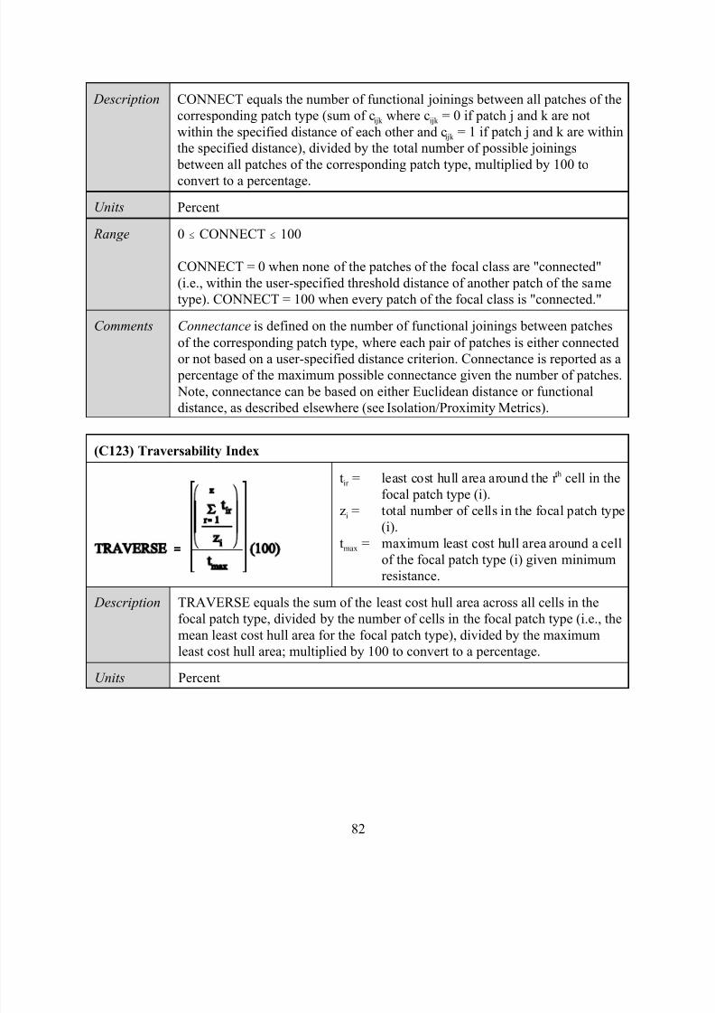
7/14/2019 Bothanical_Metrics
http://slidepdf.com/reader/full/bothanicalmetrics 82/99
82
Description CONNECT equals the number of functional joinings between all patches of the
corresponding patch type (sum of cijk where cijk = 0 if patch j and k are not
within the specified distance of each other and cijk = 1 if patch j and k are within
the specified distance), divided by the total number of possible joinings
between all patches of the corresponding patch type, multiplied by 100 to
convert to a percentage.
Units Percent
Range 0 # CONNECT # 100
CONNECT = 0 when none of the patches of the focal class are "connected"
(i.e., within the user-specified threshold distance of another patch of the same
type). CONNECT = 100 when every patch of the focal class is "connected."
Comments Connectance is defined on the number of functional joinings between patches
of the corresponding patch type, where each pair of patches is either connected
or not based on a user-specified distance criterion. Connectance is reported as a percentage of the maximum possible connectance given the number of patches.
Note, connectance can be based on either Euclidean distance or functional
distance, as described elsewhere (see Isolation/Proximity Metrics).
(C123) Traversability Index
tir = least cost hull area around the r th cell in the
focal patch type (i).
zi = total number of cells in the focal patch type
(i).tmax = maximum least cost hull area around a cell
of the focal patch type (i) given minimum
resistance.
Description TRAVERSE equals the sum of the least cost hull area across all cells in the
focal patch type, divided by the number of cells in the focal patch type (i.e., the
mean least cost hull area for the focal patch type), divided by the maximum
least cost hull area; multiplied by 100 to convert to a percentage.
Units Percent
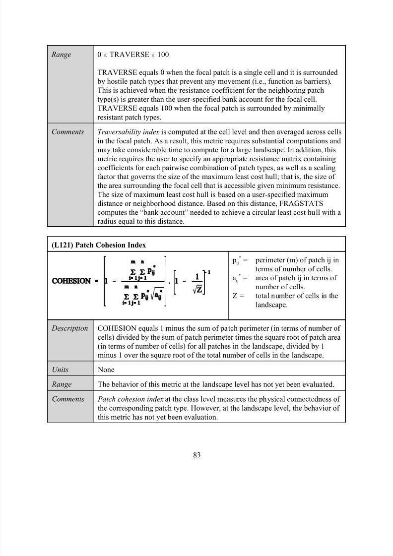
7/14/2019 Bothanical_Metrics
http://slidepdf.com/reader/full/bothanicalmetrics 83/99
83
Range 0 # TRAVERSE # 100
TRAVERSE equals 0 when the focal patch is a single cell and it is surrounded
by hostile patch types that prevent any movement (i.e., function as barriers).
This is achieved when the resistance coefficient for the neighboring patch
type(s) is greater than the user-specified bank account for the focal cell.TRAVERSE equals 100 when the focal patch is surrounded by minimally
resistant patch types.
Comments Traversability index is computed at the cell level and then averaged across cells
in the focal patch. As a result, this metric requires substantial computations and
may take considerable time to compute for a large landscape. In addition, this
metric requires the user to specify an appropriate resistance matrix containing
coefficients for each pairwise combination of patch types, as well as a scaling
factor that governs the size of the maximum least cost hull; that is, the size of
the area surrounding the focal cell that is accessible given minimum resistance.
The size of maximum least cost hull is based on a user-specified maximumdistance or neighborhood distance. Based on this distance, FRAGSTATS
computes the “bank account” needed to achieve a circular least cost hull with a
radius equal to this distance.
(L121) Patch Cohesion Index
pij
* = perimeter (m) of patch ij in
terms of number of cells.
aij* = area of patch ij in terms of
number of cells.
Z = total number of cells in the
landscape.
Description COHESION equals 1 minus the sum of patch perimeter (in terms of number of
cells) divided by the sum of patch perimeter times the square root of patch area
(in terms of number of cells) for all patches in the landscape, divided by 1
minus 1 over the square root of the total number of cells in the landscape.
Units None
Range The behavior of this metric at the landscape level has not yet been evaluated.
Comments Patch cohesion index at the class level measures the physical connectedness of
the corresponding patch type. However, at the landscape level, the behavior of
this metric has not yet been evaluation.
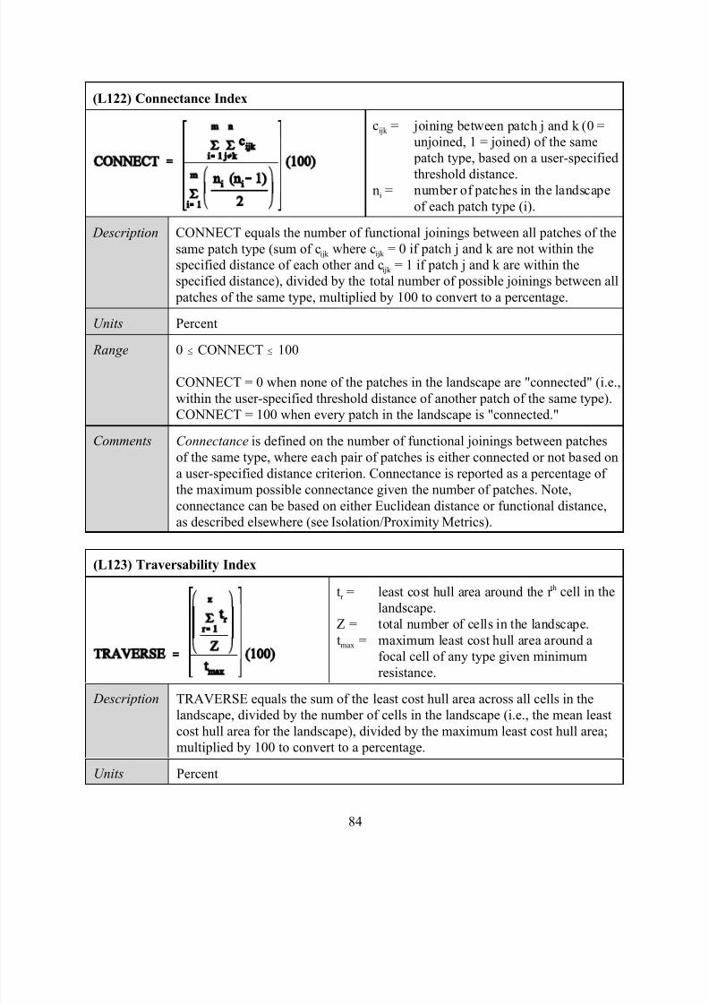
7/14/2019 Bothanical_Metrics
http://slidepdf.com/reader/full/bothanicalmetrics 84/99
84
(L122) Connectance Index
cijk = joining between patch j and k (0 =
unjoined, 1 = joined) of the same
patch type, based on a user-specified
threshold distance.ni = number of patches in the landscape
of each patch type (i).
Description CONNECT equals the number of functional joinings between all patches of the
same patch type (sum of cijk where cijk = 0 if patch j and k are not within the
specified distance of each other and cijk = 1 if patch j and k are within the
specified distance), divided by the total number of possible joinings between all
patches of the same type, multiplied by 100 to convert to a percentage.
Units Percent
Range 0 # CONNECT # 100
CONNECT = 0 when none of the patches in the landscape are "connected" (i.e.,
within the user-specified threshold distance of another patch of the same type).
CONNECT = 100 when every patch in the landscape is "connected."
Comments Connectance is defined on the number of functional joinings between patches
of the same type, where each pair of patches is either connected or not based on
a user-specified distance criterion. Connectance is reported as a percentage of
the maximum possible connectance given the number of patches. Note,
connectance can be based on either Euclidean distance or functional distance,
as described elsewhere (see Isolation/Proximity Metrics).
(L123) Traversability Index
tr = least cost hull area around the r th cell in the
landscape.
Z = total number of cells in the landscape.
tmax = maximum least cost hull area around a
focal cell of any type given minimum
resistance.
Description TRAVERSE equals the sum of the least cost hull area across all cells in thelandscape, divided by the number of cells in the landscape (i.e., the mean least
cost hull area for the landscape), divided by the maximum least cost hull area;
multiplied by 100 to convert to a percentage.
Units Percent
7/14/2019 Bothanical_Metrics
http://slidepdf.com/reader/full/bothanicalmetrics 85/99
85
Range 0 # TRAVERSE # 100
TRAVERSE equals 0 when every cell is a separate patch and is surrounded by
hostile patch types that prevent any movement (i.e., function as barriers). This
is achieved when the resistance coefficients for all patch type(s) are greater than
the user-specified bank account. TRAVERSE equals 100 when every cell issurrounded by minimally resistant patch types. This can occur when the
landscape consists of a single patch type or when all resistance coefficients are
set to the minimum value. However, in the latter case, the use of this metric
would be pointless.
Comments Traversability index is computed at the cell level and then averaged across cells
in the landscape. As a result, this metric requires substantial computations and
may take considerable time to compute for a large landscape. In addition, this
metric requires the user to specify an appropriate resistance matrix containing
coefficients for each pairwise combination of patch types, as well as a scaling
factor that governs the size of the maximum least cost hull; that is, the size of the area surrounding the focal cell that is accessible given minimum resistance.
The size of maximum least cost hull is based on a user-specified maximum
distance or neighborhood distance. Based on this distance, FRAGSTATS
computes the “bank account” needed to achieve a circular least cost hull with a
radius equal to this distance.
DIVERSITY METRICS
Background.–Diversity measures have been used extensively in a variety of ecological
applications. They originally gained popularity as measures of plant and animal species diversity.
There has been a proliferation of diversity indices and we will make no attempt to review them
here. FRAGSTATS computes 3 diversity indices. These diversity measures are influenced by 2
components--richness and evenness. Richness refers to the number of patch types present;
evenness refers to the distribution of area among different types. Richness and evenness are
generally referred to as the compositional and structural components of diversity, respectively.
Some indices (e.g., Shannon's diversity index) are more sensitive to richness than evenness.
Thus, rare patch types have a disproportionately large influence on the magnitude of the index.
Other indices (e.g., Simpson's diversity index) are relatively less sensitive to richness and thus
place more weight on the common patch types. These diversity indices have been applied by
landscape ecologists to measure one aspect of landscape structure--landscape composition (e.g.,Romme 1982, O'Neill et al. 1988, Turner 1990a).
FRAGSTATS Metrics.–FRAGSTATS computes several statistics that quantify diversity at the
landscape level. These metrics quantify landscape composition at the landscape level; they are
not affected by the spatial configuration of patches. The most popular diversity index is
7/14/2019 Bothanical_Metrics
http://slidepdf.com/reader/full/bothanicalmetrics 86/99
86
Shannon's diversity index (SHDI) based on information theory (Shannon and Weaver 1949). The
value of this index represents the amount of "information" per individual (or patch, in this case).
Information is a somewhat abstract mathematical concept that we will not attempt to define. The
absolute magnitude of Shannon's diversity index is not particularly meaningful; therefore, it is
used as a relative index for comparing different landscapes or the same landscape at different
times. Simpson's diversity index (SIDI) is another popular diversity measure that is not based oninformation theory (Simpson 1949). Simpson's index is less sensitive to the presence of rare
types and has an interpretation that is much more intuitive than Shannon's index. Specifically, the
value of Simpson's index represents the probability that any types selected at random would be
different types. Thus, the higher the value the greater the likelihood that any 2 randomly drawn
patches would be different patch types (i.e., greater diversity. Because Simpson's index is a
probability, it can be interpreted in both absolute and relative terms. FRAGSTATS also
computes a modified Simpson's diversity index (MSIDI) based on Pielou's (1975) modification of
Simpson's diversity index; this index was used by Romme (1982). The modification eliminates
the intuitive interpretation of Simpson's index as a probability, but transforms the index into one
that belongs to a general class of diversity indices to which Shannon's diversity index belongs
(Pielou 1975). Thus, the modified Simpson's and Shannon's diversity indices are similar in manyrespects and have the same applicability.
Patch richness (PR) measures the number of patch types present; it is not affected by the relative
abundance of each patch type or the spatial arrangement of patches. Therefore, two landscapes
may have very different structure yet have the same richness. For example, one landscape may be
comprised of 96% patch type A and 1% each of patch types B-E, whereas another landscape may
be comprised of 20% each of patch types A-E. Although, patch richness would be the same, the
functioning of these landscapes and the structure of the animal and plant communities would
likely be greatly different. Because richness does not account for the relative abundance of each
patch type, rare patch types and common patch types contribute equally to richness.
Nevertheless, patch richness is a key element of landscape structure because the variety of landscape elements present in a landscape can have an important influence on a variety of
ecological processes. Because many organisms are associated with a single patch type, patch
richness often correlates well with species richness.
Richness is partially a function of scale. Larger areas are generally richer because there is
generally greater heterogeneity over larger areas than over comparable smaller areas. This
contributes to the species-area relationship predicted by island biogeographic theory (MacArthur
and Wilson 1967). Therefore, comparing richness among landscapes that vary in size can be
problematic. Patch richness density (PRD) standardizes richness to a per area basis that
facilitates comparison among landscapes, although it does not correct for this interaction with
scale. FRAGSTATS also computes a relative richness index. Relative patch richness (RPR) issimilar to patch richness, but it represents richness as a percentage of the maximum potential
richness as specified by the user (Romme 1982). This form may have more interpretive value
than absolute richness or richness density in some applications. Note that relative patch richness
and patch richness are completely redundant and would not be used simultaneously in any
subsequent statistical analysis.
7/14/2019 Bothanical_Metrics
http://slidepdf.com/reader/full/bothanicalmetrics 87/99
87
Evenness measures the other aspect of landscape diversity--the distribution of area among patch
types. There are numerous ways to quantify evenness and most diversity indices have a
corresponding evenness index derived from them. In addition, evenness can be expressed as its
compliment--dominance (i.e., evenness = 1 - dominance). Indeed, dominance has often been the
chosen form in landscape ecological investigations (e.g., O'Neill et al. 1988, Turner et al. 1989,
Turner 1990a), although we prefer evenness because larger values imply greater landscapediversity. FRAGSTATS computes 3 evenness indices (Shannon's evenness index, SHEI;
Simpson's evenness index, SIEI; modified Simpson's evenness index, MSIEI), corresponding to
the 3 diversity indices. Each evenness index isolates the evenness component of diversity by
controlling for the contribution of richness to the diversity index. Evenness is expressed as the
observed level of diversity divided by the maximum possible diversity for a given patch richness.
Maximum diversity for any level of richness is based on an equal distribution among patch types.
Therefore, the observed diversity divided by the maximum diversity (i.e., equal distribution) for
a given number of patch types represents the proportional reduction in the diversity index
attributed to lack of perfect evenness. As the evenness index approaches 1, the observed diversity
approaches perfect evenness. Because evenness is represented as a proportion of maximum
evenness, Shannon's evenness index does not suffer from the limitation of Shannon's diversityindex with respect to interpretability.
Limitations.–The use of diversity measures in community ecology has been heavily criticized
because diversity conveys no information on the actual species composition of a community.
Species diversity is a community summary measure that does not take into account the
uniqueness or potential ecological, social, or economical importance of individual species. A
community may have high species diversity yet be comprised largely of common or undesirable
species. Conversely, a community may have low species diversity yet be comprised of especially
unique, rare, or highly desired species. Although these criticisms have not been discussed
explicitly with regards to the landscape ecological application of diversity measures, these
criticisms are equally valid when diversity measures are applied to patch types instead of species.In addition, diversity indices like Shannon’s index and Simpson’s index combine richness and
evenness components into a single measure, even though it is usually more informative to
evaluate richness and evenness independently.
Code Metric (acronym)
Landscape Metrics
L124 Patch Richness (PR)
L125 Patch Rich nes s Density ( PRD)
L126 Relativ e Patch Richn ess (RPR)
L127 Shanno n’s Diversity Index (SHD I)
L128 Simpson ’s Diversity Index (SIDI)
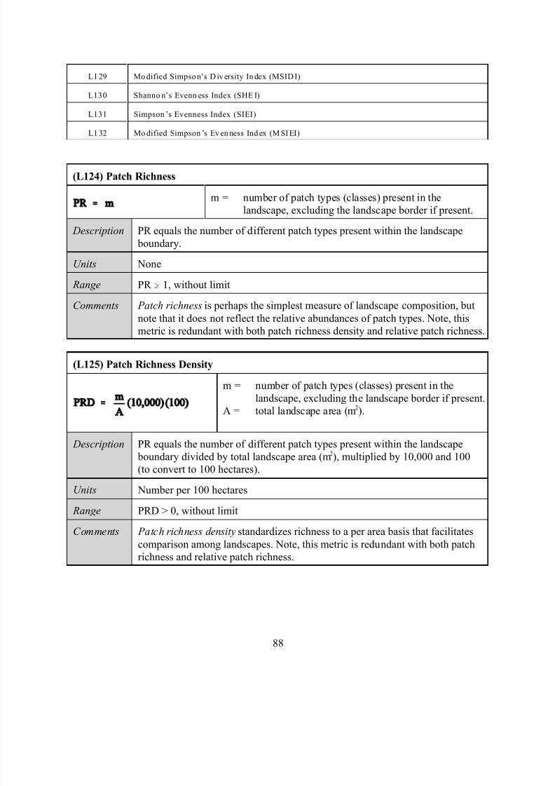
7/14/2019 Bothanical_Metrics
http://slidepdf.com/reader/full/bothanicalmetrics 88/99
88
L1 29 Mo dified Simpso n’s D iv ersity In dex (MSID I)
L130 Shanno n’s Evenn ess Index (SHE I)
L131 Simpson ’s Evenness Index (SIEI)
L1 32 Mo dified Simpson ’s Ev en ness Ind ex (M SI EI)
(L124) Patch Richness
m = number of patch types (classes) present in the
landscape, excluding the landscape border if present.
Description PR equals the number of different patch types present within the landscape
boundary.
Units None
Range PR $ 1, without limit
Comments Patch richness is perhaps the simplest measure of landscape composition, but
note that it does not reflect the relative abundances of patch types. Note, this
metric is redundant with both patch richness density and relative patch richness.
(L125) Patch Richness Density
m = number of patch types (classes) present in the
landscape, excluding the landscape border if present.
A = total landscape area (m2
).
Description PR equals the number of different patch types present within the landscape
boundary divided by total landscape area (m2), multiplied by 10,000 and 100
(to convert to 100 hectares).
Units Number per 100 hectares
Range PRD > 0, without limit
Comments Patch richness density standardizes richness to a per area basis that facilitates
comparison among landscapes. Note, this metric is redundant with both patch
richness and relative patch richness.

7/14/2019 Bothanical_Metrics
http://slidepdf.com/reader/full/bothanicalmetrics 89/99
89
(L126) Relative Patch Richness
m = number of patch types (classes) present in
the landscape, excluding the landscape
border if present.
Description RPR equals the number of different patch types present within the landscape
boundary divided by the maximum potential number of patch types specified
by the user, based on the particular patch type classification scheme, multiplied
by 100 (to convert to percent).
Units Percent
Range 0 < RPR # 100
RPR approaches 0 when the landscape contains a single patch type, yet the
number of potential patch types is very large. RPR = 100 when all possible
patch types are represented in the landscape.
Comments Relative patch richness is similar to patch richness, but it represents richness as
a percentage of the maximum potential richness as specified by the user. Note,
this metric is redundant with both patch richness and patch richness density.
(L127) Shannon's Diversity Index
Pi = proportion of the landscape occupied by patch
type (class) i.
Description SHDI equals minus the sum, across all patch types, of the proportional
abundance of each patch type multiplied by that proportion.
Units Information
Range SHDI $ 0, without limit
SHDI = 0 when the landscape contains only 1 patch (i.e., no diversity). SHDI
increases as the number of different patch types (i.e., patch richness, PR)
increases and/or the proportional distribution of area among patch types
becomes more equitable.
Comments Shannon’s diversity index is a popular measure of diversity in community
ecology, applied here to landscapes. Shannon’s index is somewhat more
sensitive to rare patch types than Simpson’s diversity index.
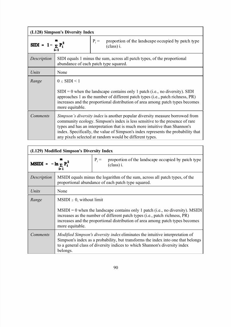
7/14/2019 Bothanical_Metrics
http://slidepdf.com/reader/full/bothanicalmetrics 90/99
90
(L128) Simpson's Diversity Index
Pi = proportion of the landscape occupied by patch type
(class) i.
Description SIDI equals 1 minus the sum, across all patch types, of the proportionalabundance of each patch type squared.
Units None
Range 0 # SIDI < 1
SIDI = 0 when the landscape contains only 1 patch (i.e., no diversity). SIDI
approaches 1 as the number of different patch types (i.e., patch richness, PR)
increases and the proportional distribution of area among patch types becomes
more equitable.
Comments Simpson’s diversity index is another popular diversity measure borrowed fromcommunity ecology. Simpson's index is less sensitive to the presence of rare
types and has an interpretation that is much more intuitive than Shannon's
index. Specifically, the value of Simpson's index represents the probability that
any pixels selected at random would be different types.
(L129) Modified Simpson's Diversity Index
Pi = proportion of the landscape occupied by patch type
(class) i.
Description MSIDI equals minus the logarithm of the sum, across all patch types, of the
proportional abundance of each patch type squared.
Units None
Range MSIDI $ 0, without limit
MSIDI = 0 when the landscape contains only 1 patch (i.e., no diversity). MSIDI
increases as the number of different patch types (i.e., patch richness, PR)
increases and the proportional distribution of area among patch types becomes
more equitable.
Comments Modified Simpson's diversity index eliminates the intuitive interpretation of
Simpson's index as a probability, but transforms the index into one that belongs
to a general class of diversity indices to which Shannon's diversity index
belongs.
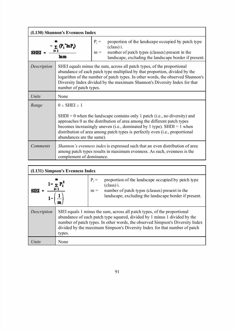
7/14/2019 Bothanical_Metrics
http://slidepdf.com/reader/full/bothanicalmetrics 91/99
91
(L130) Shannon's Evenness Index
Pi = proportion of the landscape occupied by patch type
(class) i.
m = number of patch types (classes) present in the
landscape, excluding the landscape border if present.
Description SHEI equals minus the sum, across all patch types, of the proportional
abundance of each patch type multiplied by that proportion, divided by the
logarithm of the number of patch types. In other words, the observed Shannon's
Diversity Index divided by the maximum Shannon's Diversity Index for that
number of patch types.
Units None
Range 0 # SHEI # 1
SHDI = 0 when the landscape contains only 1 patch (i.e., no diversity) andapproaches 0 as the distribution of area among the different patch types
becomes increasingly uneven (i.e., dominated by 1 type). SHDI = 1 when
distribution of area among patch types is perfectly even (i.e., proportional
abundances are the same).
Comments Shannon’s evenness index is expressed such that an even distribution of area
among patch types results in maximum evenness. As such, evenness is the
complement of dominance.
(L131) Simpson's Evenness Index
Pi = proportion of the landscape occupied by patch type
(class) i.
m = number of patch types (classes) present in the
landscape, excluding the landscape border if present.
Description SIEI equals 1 minus the sum, across all patch types, of the proportional
abundance of each patch type squared, divided by 1 minus 1 divided by the
number of patch types. In other words, the observed Simpson's Diversity Index
divided by the maximum Simpson's Diversity Index for that number of patch
types.
Units None
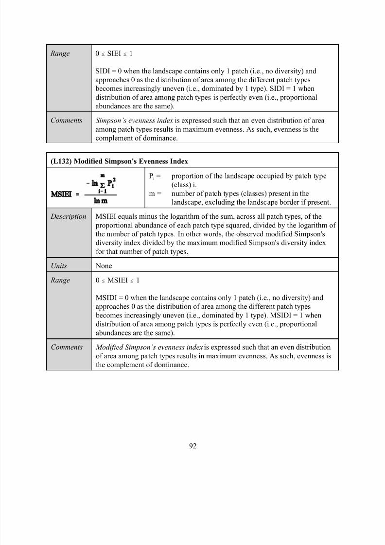
7/14/2019 Bothanical_Metrics
http://slidepdf.com/reader/full/bothanicalmetrics 92/99
92
Range 0 # SIEI # 1
SIDI = 0 when the landscape contains only 1 patch (i.e., no diversity) and
approaches 0 as the distribution of area among the different patch types
becomes increasingly uneven (i.e., dominated by 1 type). SIDI = 1 when
distribution of area among patch types is perfectly even (i.e., proportionalabundances are the same).
Comments Simpson’s evenness index is expressed such that an even distribution of area
among patch types results in maximum evenness. As such, evenness is the
complement of dominance.
(L132) Modified Simpson's Evenness Index
Pi = proportion of the landscape occupied by patch type
(class) i.
m = number of patch types (classes) present in thelandscape, excluding the landscape border if present.
Description MSIEI equals minus the logarithm of the sum, across all patch types, of the
proportional abundance of each patch type squared, divided by the logarithm of
the number of patch types. In other words, the observed modified Simpson's
diversity index divided by the maximum modified Simpson's diversity index
for that number of patch types.
Units None
Range 0 # MSIEI # 1
MSIDI = 0 when the landscape contains only 1 patch (i.e., no diversity) and
approaches 0 as the distribution of area among the different patch types
becomes increasingly uneven (i.e., dominated by 1 type). MSIDI = 1 when
distribution of area among patch types is perfectly even (i.e., proportional
abundances are the same).
Comments Modified Simpson’s evenness index is expressed such that an even distribution
of area among patch types results in maximum evenness. As such, evenness is
the complement of dominance.
7/14/2019 Bothanical_Metrics
http://slidepdf.com/reader/full/bothanicalmetrics 93/99
93
LITERATURE CITED
Brittingham, M. C., and S. A. Temple. 1983. Have cowbirds caused forest songbirds to decline?
Bio-Science 33:31-35.
Baker, W. L., and Y. Cai. 1992. The r.le programs for multiscale analysis of landscape structureusing the GRASS geographical information system. Landscape Ecology 7: 291-302.
Bendell, P. R., and J. E. Gates. 1987. Home range and microhabitat partitioning of the southern
flying squirrel (Glaucomy volans). J. Mammology 68:243-255.
Buechner, M. 1989. Are small-scale landscape features important factors for field studies of
small mammal dispersal sinks? Landscape Ecology 2:191-199.
Burrough, P. A. 1986. Principles of Geographical Information Systems for Land Resources
Assessment. Clarendon Press, Oxford.
Chasko, G. G, J. E. Gates. 1982. Avian habitat suitability along a transmission-line corridor in an
oak-hickory forest region. Wildl. Monogr. 82.
Chen, J., and J. F. Franklin. 1990. Microclimatic pattern and basic biological responses at the
clearcut edges of old-growth Douglas-fir stands. Northwest Environ. J. 6:424-425.
Dale, M. R. T. 2000. Lacunarity analysis of spatial pattern: a comparison. Landscape Ecol.
15:467-468.
Dale, V. H., S. M. Pearson, H. L. Oferman, and R. V. O’Neill. 1994. Relating patterns of land-
use change to faunal biodiversity in the central Amazon. Conservation Biology 8:1027-1036.
Dickman, C. R. 1987. Habitat fragmentation and vertebrate species richness in an urban
environment. J. Appl. Ecol. 24:337-351.
Dunning, J. B., B. J. Danielson, and H. R. Pulliam. 1992. Ecological processes that affect
populations in complex landscapes. Oikos 65:169-175.
Forman, R. T. T., A. E. Galli, and C. F. Leck. 1976. Forest size and avian diversity in New
Jersey woodlots with some land use implications. Oecologia 26:1-8.
Forman, R. T. T., and M. Godron. 1986. Landscape Ecology. John Wiley & Sons, New York.619 pp.
Forsman, E. D., E. C. Meslow, and H. M. Wight. 1984. Distribution and biology of the spotted
owl in Oregon. Wildl. Monogr. 87. 64 pp.
7/14/2019 Bothanical_Metrics
http://slidepdf.com/reader/full/bothanicalmetrics 94/99
94
Franklin, J. F., and R. T. T. Forman. 1987. Creating landscape pattern by forest cutting:
ecological consequences and principles. Landscape Ecology 1:5-18.
Gardner, R. H., B. T. Milne, M.G. Turner, and R.V. O'Neill. 1987. Neutral models for the
analysis of broad-scale landscape pattern. Landscape Ecol. 1:19-28.
Gardner, R. H., and R. V. O’Neill. 1991. Pattern, process, and predictability: the use of neutral
models for landscape analysis. Pages 289-307 In M. G. Turner and R. H. Gardner, eds.
Quantitative Methods in Landscape Ecology. Springer-Verlag, New York.
Gilpin, M. E., and I. Hanski (eds). 1991. Metapopulation Dynamics: Empirical and Theoretical
Investigations. Academic Press, San Diego. 336 pp.
Graham, R. L., C. T. Hunsaker, R. V., O'Neill, and B. Jackson. 1991. Ecological risk assessment
at the regional scale. Ecol. Appl. 1:196-206.
Gratkowski, H. J. 1956. Windthrow around staggered settings in old-growth Douglas-fir. For.Sci. 2:60-74.
Gustafson, E. J. 1998. Quantifying landscape spatial pattern: What is the state of the art.
Ecosystems:143-156.
Gustafson, E. J., and G. R. Parker. 1994. Using an index of habitat patch proximity for landscape
design. Landscape and Urban Planning 29:117-30.
Gustafson, E. J., G. R. Parker, and S. E. Backs. 1994. Evaluating spatial pattern of wildlife
habitat: a case study of the wild turkey (Meleagris gallopavo). Am. Midl. Nat. 131:24-33.
Gustafson, E. J., and G. R. Parker. 1992. Relationships between landcover proportion and indices
of landscape spatial pattern. Landscape Ecology 7:101-110.
Hansen, A., and F. di Castri (eds). 1992. Landscape Boundaries. Springer, New York.
Hardt, R. A., and R. T. T. Forman. 1989. Boundary form effects on woody colonization of
reclaimed surface mines. Ecology 70:1252-1260.
Hargis, C. D., J. A. Bissonette, and J. L. David. 1998. The behavior of landscape metrics
commonly used in the study of habitat fragmentation. Landscape Ecol. 13:167-186.
Hayden, I. J., J. Faaborg, and R. L. Clawson. 1985. Estimates of minimum area requirements for
Missouri forest birds. Missouri Academy of Science 19:11-22.
Helliwell, D. R. 1976. The effects of size and isolation on the conservation value of wooded sites
in Britain. J. Biogeogr. 3:407-416.

7/14/2019 Bothanical_Metrics
http://slidepdf.com/reader/full/bothanicalmetrics 95/99
95
Iverson, L. R. 1989. Land use changes in Illinois, USA: the influence of landscape attributes on
current and historic land use. Landscape Ecology 2:45-61.
Jaeger, J. A. G. 2000. Landscape division, splitting index, and effective mesh size: new measures
of landscape fragmentation. Landscape Ecol. 15:115-130.
Kareiva, P. 1990. Population dynamics in spatially complex environments: theory and data. Phil.
Trans. R. Soc. Lond. B 330:175-190.
Keitt, T.H., D.L. Urban, and B.T. Milne. 1997. Detecting critical scales in fragmented
landscapes. Conservation Ecol. 1(1):4. (online)
Kotliar, N. B., and J. A. Wiens. 1990. Multiple scales of patchiness and patch structure: a
hierarchical framework for the study of heterogeneity. Oikos 59:253-260.
Kremsater, L. and F. L. Bunnell.1999. Edge effects: theory, evidence and implications to
management of western North American forests.
Kroodsma, R. L. 1982. Edge effect on breeding forest birds along a power-line corridor. J. of
Applied Ecology 19:361-370.
Krummel, J. R., R. H. Gardner, G. Sugihara, R. V. O'Neill, and P. R. Coleman. 1987. Landscape
patterns in a disturbed environment. Oikos 48:321-324.
Lamberson, R.H., R. McKelvey, B.R. Noon, and C. Voss. 1992. A dynamic analysis of northern
spotted owl viability in a fragmented forest landscape. Conservation Biology 6(4):1-8.
LaGro, J., Jr. 1991. Assessing patch shape in landscape mosaics. Photogrammetric Eng. RemoteSens. 57:285-93.
Lande, R. 1987. Extinction thresholds in demographic models of territorial populations.
American Naturalist 130:624-635.
Lehmkuhl, J. F., and M. G. Raphael. 1993. Habitat pattern around northern spotted owl locations
on the Olympic Peninsula, Washington. J. Wildl. Manage. 57:302-315.
Leopold, A. 1933. Game Management. Charles Scribners, New York.
Levins, R. 1970. Extinctions. Pages 77-107 In M. Gertenhaber, ed. Some MathematicalQuestions in Biology, vol 2. Lectures on Mathematics in the Life Sciences. Amer. Math. Soc.,
Providence, Rhode Island.
Li, H., and J. F. Reynolds. 1993. A new contagion index to quantify spatial patterns of
landscapes. Landscape Ecology 8:155-162.
7/14/2019 Bothanical_Metrics
http://slidepdf.com/reader/full/bothanicalmetrics 96/99
96
Logan, W., E. R. Brown, D. Longrie, G. Herb, and R. A. Corthell. 1985. Edges. Pages 115-127
In E. R. Brown, tech. ed. Management of wildlife and fish habitats in forests of western Oregon
and Washington. USDA For. Serv. Publ. No. R6-F&WL-192-1985.
MacArthur, R. H., and E. O. Wilson. 1967. The Theory of Island Biogeography. Princeton
University Press, Princeton. 203 pp.
Mandelbrot, B. B. 1982. The Fractal Geometry of Nature. W. H. Freeman and Co., New York.
Mandelbrot, B. B. 1977. Fractals, Form, Chance and Dimension. W. H. Freeman and Co., New
York.
Mader, H-J. 1984. Animal habitat isolation by roads and agricultural fields. Biological
Conservation 29:81-96.
McKelvey, K., B.R. Noon, and R. Lamberson. 1992. Conservation planning for species
occupying fragmented landscapes: the case of the northern spotted owl. Pages 338-357 In J.Kingsolver, P. Kareiva, and R. Hyey, eds. Biotic interactions and global change. Sinauer
Associates, Sunderland, MA.
Milne, B. T. 1988. Measuring the fractal geometry of landscapes. Applied Mathematics and
Computation 27:67-79.
Moore, N. W., and M. D. Hooper. 1975. On the number of bird species in British woods. Biol.
Conserv. 8:239-250.
Morgan, K. A., and J. E. Gates. 1982. Bird population patterns in forest edge and strip vegetation
at Remington Farms, Maryland. J. Wildl. Manage. 46:933-944.
Noss, R. F. 1988. Effects of edge and internal patchiness on habitat use by birds in a Florida
hardwood forest. Ph.D. Thesis. Univ. of Florida, Gainesville. 109 pp.
O'Neill , R. V., C. T. Hunsaker, S. P. Timmins, B. L. Jackson, K. B. Jones, K. H. Ritters, and J.
D. Wickham.1996. Scale problems in reporting landscape pattern at the regional scale.
Landscape Ecology 11:
O'Neill , R. V., J. R. Krummel, R. H. Gardner, G. Sugihara, B. Jackson, D. L. DeAngelis, B. T.
Milne, M. G. Turner, B. Zygmunt, S. W. Christensen, V. H. Dale, and R. L. Graham. 1988.
Indices of landscape pattern. Landscape Ecology 1:153-162.
Patton, D. R. 1975. A diversity index for quantifying habitat "edge". Wildl. Soc. Bull. 3:171-173.
Pearson, S. M., M. G. Turner, R. H. Gardner, and R. V. O’Neill. 1996. An organism-based
perspective of habitat fragmentation. Pages 77-95 In R. C. Szaro and D. W. Johnston, eds.
7/14/2019 Bothanical_Metrics
http://slidepdf.com/reader/full/bothanicalmetrics 97/99
97
Biodiversity in Managed Landscapes: Theory and Practice. Oxford University Press, New York.
Pielou, E. C. 1975. Ecological Diversity. Wiley-Interscience, New York.
Plotnick, R. E., R. H. Gardner, and R.V. O'Neill. 1993. Lacunarity indices as measures of
landscape texture. Landscape Ecol. 8:201-211.
Plotnick, R. E., R. H. Gardner, W. W. Hargrove, K. Pretegaard, and M. Perlmutter.1996.
Lacunarity analysis: a general technique for the analysis of spatial patterns. Phys. Rev.
E53:5461-5468.
Ranney, J. W., M. C. Bruner, and J. B. Levenson. 1981. The importance of edge in the structure
and dynamics of forest islands. Pages 67-94 In R. L. Burgess and D. M. Sharpe, eds. Forest
Island Dynamics in Man-Dominated Landscapes. Springer-Verlag, New York.
Ripple, W. J., G. A. Bradshaw, and T. A. Spies. 1991. Measuring landscape pattern in the
Cascade Range of Oregon, USA. Biological Conserv. 57:73-88.
Ritters, K. H., R. V. O'Neill, C. T. Hunsaker, J. D. Wickham, D. H. Yankee, S. P. Timmins, K.
B. Jones, and B. L. Jackson. 1995. A factor analysis of landscape pattern and structure metrics.
Landscape Ecol. 10: 23-40.
Ritters, K. H., R. V. O'Neill, J. D. Wickham, and K. B. Jones. 1996. A note on contagion indices
for landscape analysis. Landscape Ecol. 11:197-202.
Robbins, C. S., D. K. Dawson, and B. A. Dowell. 1989. Habitat area requirements of breeding
forest birds of the middle Atlantic states. Wildl. Monogr.103. 34 pp.
Rogers, C. A. 1993. Describing landscapes: indices of structure. M.S. Thesis, Simon Fraser
University, Burnaby, British Columbia. 170 pp.
Romme, W. H. 1982. Fire and landscape diversity in subalpine forests of Yellowstone National
Park. Ecol. Monogr. 52:199-221.
Saunders, D., R. J. Hobbs, and C. R. Margules. 1991. Biological consequences of ecosystem
fragmentation: a review. Conserv. Biol. 5:18-32.
Schumaker, N. H. 1996. Using landscape indices to predict habitat connectivity. Ecology
77:1210-25.
Shannon, C., and W. Weaver. 1949. The mathematical theory of communication. Univ. Illinois
Press, Urbana.
Simpson, E. H. 1949. Measurement of diversity. Nature 163:688.
7/14/2019 Bothanical_Metrics
http://slidepdf.com/reader/full/bothanicalmetrics 98/99
98
Stauffer, D. 1985. Introduction to Percolation Theory. Taylor and Francis, London.
Strelke, W. K., and J. G. Dickson. 1980. Effect of forest clearcut edge on breeding birds in
Texas. J. Wildl. Manage. 44:559-567.
Taylor, P. D., L. Fahrig, K. Henein, and G. Merriam. 1993. Connectivity is a vital element of landscape structure. Oikos 73:43-48.
Temple, S. A. 1986. Predicting impacts of habitat fragmentation on forest birds: a comparison of
two models. Pages 301-304 In J. Verner, M. L. Morrison, and C. J. Ralph, eds. Wildlife 2000:
Modeling Habitat Relationships of Terrestrial Vertebrates. Univ. of Wisconsin Press, Madison,
WI.
Thomas, J. W., C. Maser, and J. E. Rodiek. 1979. Edges. Pages 48-59 In J. W. Thomas, tech. ed.
Wildlife habitats in managed forests, the Blue Mountains of Oregon and Washington. USDA
For. Serv. Handb. 553.
Thomas, J. W., C. Maser, and J. E. Rodiek. 1978. Edges--their interspersion, resulting diversity,
and its measurement. Pages 91-100 In R. M. Degraff, tech. coord. Proceedings of the workshop
on nongame bird habitat management in the coniferous forests of the western United States. Gen.
Tech. Rep. PNW-64.
Turner, M. G. 1989. Landscape ecology: the effect of pattern on process. Ann. Rev. Ecol. Syst.
20:171-197.
Turner, M. G. 1990a. Spatial and temporal analysis of landscape patterns. Landscape Ecology
4:21-30.
Turner, M. G. 1990b. Landscape changes in nine rural counties of Georgia. Photogram. Engine.
and Rem. Sens. 56:379-386.
Turner, M. G., R. V. O'Neill, R. H. Gardner, and B. T. Milne. 1989. Effects of changing spatial
scale on the analysis of landscape pattern. Landscape Ecology 3:153-162.
Turner, M. G., and C. L. Ruscher. 1988. Changes in the spatial patterns of lands use in Georgia.
Landscape Ecology 1:241-251.
Voss, R. F. 1988. Fractals in nature: from characterization to simulation. Pages 21-70 In H.O.
Petigen and D. Saupe, eds. The Science of Fractal Images. Springer-Verlag, New York.
Wegner, J. F., and H. G. Merriam. 1979. Movements by birds and small mammals between a
wood and adjoining farmland habitats. J. Appl. Ecol. 16:349-357.
Whitcomb, R. F., C. S. Robbins, J. F. Lynch, B. L. Whitcomb, M. K. Klimkiewicz, and D
7/14/2019 Bothanical_Metrics
http://slidepdf.com/reader/full/bothanicalmetrics 99/99
Bystrak. 1981. Effects of forest fragmentation on avifauna of the eastern deciduous forest. Pages
125-205 in R. L. Burgess and D. M. Sharpe, eds. Forest Island Dynamics in Man-Dominated
Landscapes. Springer-Verlag, New York.
Wiens, J. A., C. S. Crawford, and J. R. Gosz. 1985. Boundary dynamics: a conceptual framework
for studying landscape ecosystems. Oikos 45: 421-427.
Wilcove, D. S. 1985. Nest predation in forest tracts and the decline of migratory songbirds.
Ecology 66:1211-1214.
With, K. A. 1999. Is landscape connectivity necessary and sufficient for wildlife management?
Pages 97-115 in J. A. Rochelle, L. A. Lehmann, and J. Wisniewski, editors. Forest
fragmentation: wildlife and management implications. Brill, The Netherlands.
With, K. A., and T. O. Crist. 1995. Critical thresholds in species’ responses to landscape
structure. Ecology 76:2446-59.
With, K. A., R. H. Gardner, and M. G. Turner. 1997. Landscape connectivity and population
distributions in heterogeneous environments. Oikos 78:151-169.
With, K. A., and A.W. King. 1999a. Dispersal success on fractal landscapes: a consequence of
lacunarity thresholds. Landscape Ecology 14:73-82.
With, K. A., and A.W. King. 1999b. Extinction thresholds for species in fractal landscapes.
Conservation Biology 13:314-326.
Yahner, R. H. 1986. Spatial distribution of white-footed mice (Peromyscus leucopus) in
fragmented forest stands. Proceedings of the Pennsylvania Academy of Science 60:165-166.
Yahner, R. H., and D. P. Scott. 1988. Effects of forest fragmentation on depredation of artificial
nests. J. Wildl. Manage. 52:158-161.


