Boundary Element Method of Modelling Steady State ... · PDF fileBoundary element method of modelling steady state groundwater ow 8053 Equation (3) includes the storage term (S s @h

Applied Mathematical Sciences, Vol. 8, 2014, no. 162, 8051 - 8078

HIKARI Ltd, www.m-hikari.com

http://dx.doi.org/10.12988/ams.2014.49772

Boundary Element Method of Modelling

Steady State Groundwater Flow

D. Nkurunziza1, G. Kakuba2, J. M. Mango2, S. E. Rugeihyamu3

and N. Muyinda2

1Department of Mathematics, University of Burundi, Bujumbura, Burundi2Department of Mathematics, Makerere University, Kampala, Uganda

3Department of Mathematics, University of Dar es Salaam, Dar es Salaam, Tanzania

Copyright c© 2014 D. Nkurunziza, G. Kakuba, J. M. Mango, S. E. Rugeihyamu and N.

Muyinda. This is an open access article distributed under the Creative Commons Attribution

License, which permits unrestricted use, distribution, and reproduction in any medium,

provided the original work is properly cited.

Abstract

Water is a very important resource for any living organism and is

mainly underground. The movement of groundwater is governed by

the Laplace equation ∇2h = 0, where h is the hydraulic head. Much

research has been on groundwater modelling and many of them are in-

spired by Darcy’s law. The Boundary Element Method is one of the

few widely used numerical techniques for solving boundary value prob-

lems in engineering and physical sciences. In this study, a steady state

groundwater flow model has been analyzed using the boundary element

method. The results show that water moves from points at higher hy-

draulic head to points at lower hydraulic head. This result using the

boundary element method is in perfect agreement with the 2014 result

by the same authors using the finite volume method.

Keywords: Groundwater Flow, Boundary Element Method,Green’s Identity,

Discretization

8052 D. Nkurunziza et al.

1 Introduction

Groundwater models dictate how we translate flow systems for the calculation

of groundwater flux and head [10]. Because of the simplifying assumptions

embedded in the mathematical equations and the many uncertainties in the

values of data required by the model, a model must be viewed as an ap-

proximation and not an exact duplication of field conditions. Groundwater

models, however, even as approximations are a useful investigation tool. For

the calculations one needs hydrological inputs, hydraulic parameters, initial

and boundary conditions. The input is usually the inflow into the aquifer or

the recharge, which varies temporally and spatially[11].

Groundwater flow and transport models simulate either steady state or tran-

sient flow. In steady-state systems, inputs and outputs are in equilibrium so

that there is no net change in the system with time. In transient simulations,

the inputs and outputs are not in equilibrium so there is a net change in the

system with time. Steady state models provide average, long-term results.

Transient models should be used when the groundwater regime varies over

time[10]. Application of models to the analysis of steady flow in an aquifer

requires knowledge of the spatial distributions of transitivity, boundary con-

ditions and recharge rates with the aquifer[3]. In addition to the required

knowledge in steady modeling, the transient model needs the initial condi-

tions.

The general three-dimensional flow equation is given as:

∂

∂x

(Kx

∂h

∂x

)+

∂

∂y

(Ky

∂h

∂y

)+

∂

∂z

(Kz

∂h

∂z

)= Ss

∂h

∂t. (1)

where h is the hydraulic head, K is the hydraulic conductivity and Ss is the

specific storage coefficient. If the hydraulic conductivities are assumed to be

homogenous (Kx, Ky, Kz are independent of x, y, z), the general equation can

be written as:

Kx∂2h

∂x2+Ky

∂2h

∂y2+Kz

∂2h

∂z2= Ss

∂h

∂t. (2)

When conductivity is also isotropic, that is Kx = Ky = Kz = K, this simplifies

further to∂2h

∂x2+∂2h

∂y2+∂2h

∂z2= ∇2h =

SsK

∂h

∂t, (3)

where ∇2 =( ∂2

∂x2, ∂

2

∂y2, ∂

2

∂z2) is called the Laplacian operator.

Boundary element method of modelling steady state groundwater flow 8053

Equation (3) includes the storage term (Ss∂h∂t

) which occurs only in transient

flow when ∂h∂t6= 0 [8]. If however, the flow is steady state, ∂h

∂t= 0, the right-

hand-side of (3) become zero. Then we have:

∇2h = 0. (4)

Equation (4) is the well known Laplace equation and is the main concern in

the present study since we model steady state flow.

2 Boundary Element Discretization

The boundary element method(BEM) is a powerful technique to solve bound-

ary value problems numerically. The idea of BEM is that we can approximate

the solution to a Partial Differential Equation (PDE) by looking at the solu-

tion to the PDE on the boundary and then use that information to find the

solution in the interior of the domain [6]. The BEM is even more dominant for

problems where the solution domain extends to infinity. Such problems occur

frequently in acoustics [7]. The BEM also has wide applications in inverse

problems [5].

In the present study, the boundary element method is employed to solve the

two-dimensional Laplace Equation

∇2u(r) = 0, r = (x, y) ∈ Ω ⊂ R2 (5)

in a domain Ω, with an enclosing boundary Γ. On the boundary Γ, either

Dirichlet or Neumann boundary conditions are prescribed. Together, the gov-

erning partial differential equation within a domain and the boundary condi-

tion is called a Boundary Value Problem (BVP). The BVP can be classified

as follows:

(1) Dirichlet B.V.P

∇2u(r) = 0 in Ω ;u(r) = u(r) on Γ; (6)

(2) Neumann B.V.P

∇2u(r) = 0 in Ω ;∂u(r)

∂n= un(r) on Γ; (7)


(3) Mixed B.V.P

∇2u(r) = 0 in Ω; u(r) = u(r) on Γ1 and∂u(r)

∂n= un(r) on Γ2; (8)

where

Γ1 ∪ Γ2 =Γ and Γ1 ∩ Γ2 = ∅, u(r) and un(r) are known functions defined on

the boundary.

The solution to such a problem is principally the determination of u at points

in the domain Ω, whether by analytic or numerical methods.

2.1 Fundamental solution

Before one applies the boundary element method to a particular problem, it is a

must to obtain or know a fundamental solution for the problem. Fundamental

solutions are tied to the Dirac Delta function [2]. Consider a point source

placed at point p(x, y) of the xy-plane. Its density at r(ξ, η) may be expressed

mathematically by the delta function as

f(r) = δ(r− p) (9)

where

δ(r− p) =

1 when p ∈ Ω,

0 when p ∈ Ωc (10)

and the potential v = v(r,p) produced at point r satisfies the equation

∇2v(r,p) = δ(r− p). (11)

A singular particular solution of equation (11) is called the fundamental solu-

tion of the potential equation [13]. It is determined by writing equation (11)

in polar coordinates with origin at the point source p. Since this solution is

axisymmetric with respect to the source, it is independent of the polar angle

θ.


t

o

T

P

qQ

n

r

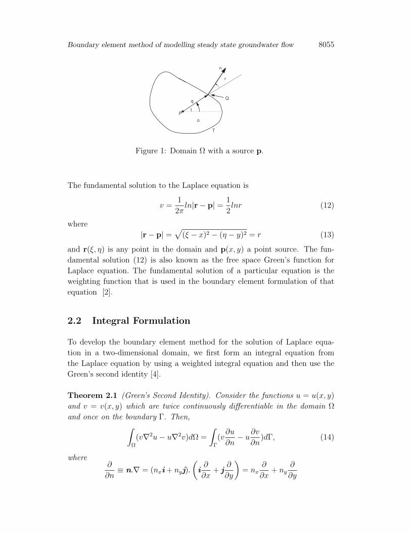
Figure 1: Domain Ω with a source p.

The fundamental solution to the Laplace equation is

v =1

2πln|r− p| = 1

2lnr (12)

where

|r− p| =√

(ξ − x)2 − (η − y)2 = r (13)

and r(ξ, η) is any point in the domain and p(x, y) a point source. The fun-

damental solution (12) is also known as the free space Green’s function for

Laplace equation. The fundamental solution of a particular equation is the

weighting function that is used in the boundary element formulation of that

equation [2].

2.2 Integral Formulation

To develop the boundary element method for the solution of Laplace equa-

tion in a two-dimensional domain, we first form an integral equation from

the Laplace equation by using a weighted integral equation and then use the

Green’s second identity [4].

Theorem 2.1 (Green’s Second Identity). Consider the functions u = u(x, y)

and v = v(x, y) which are twice continuously differentiable in the domain Ω

and once on the boundary Γ. Then,∫Ω

(v∇2u− u∇2v)dΩ =

∫Γ

(v∂u

∂n− u∂v

∂n)dΓ, (14)

where∂

∂n≡ n.∇ = (nxi + nyj).

(i∂

∂x+ j

∂

∂y

)= nx

∂

∂x+ ny

∂

∂y


is the operator that produces the derivative of a function in the direction of

n[9].

Applying Green’s identity (14), for the function u and v that satisfy equations

(5) and (11), respectively, and assuming that the source lies at point p ∈ Ω,

we obtain

−∫

Ω

u(r)δ(r− p)dΩr =

∫Γ

[v(r,p)

∂u(r)

∂nr

− u(r)∂v(r,p)

∂nr

]dsr. (15)

where p is a fixed point in Ω, r and r are variable points in Ω and in Γ

respectively.

Since v(r,p) = v(p, r) by equation (12), equation (15) is written as

−∫

Ω

u(p)δ(p− r)dΩr =

∫Γ

[v(p, r)

∂u(r)

∂nr

− u(p)∂v(p, r)

∂nr

]dsr, (16)

where δ(r− p) is the Dirac delta function in two dimension defined as

∫Ω

δ(p− r)h(p)dΩp = h(r), p(x, y), r(ξ, η) ∈ Ω (17)

for an arbitrary function h(p), which is continuous in the domain Ω containing

the point r(ξ, η).

The two-dimensional delta function may also be described by

δ(p− r) =

0 , p 6= r,

∞ , p = r,(18)

and ∫Ω

δ(p− r)dΩp =

∫Ω∗δ(p− r)dΩp = 1, r(ξ, η) ∈ Ω∗ ⊆ Ω. (19)

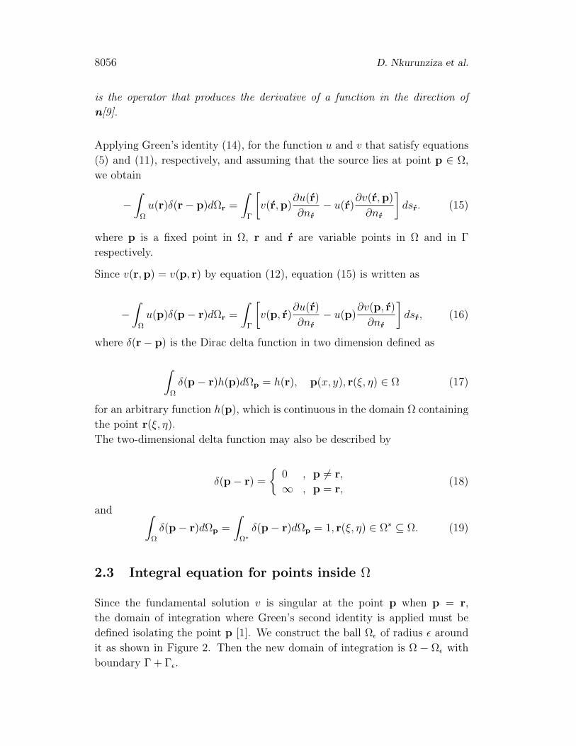
2.3 Integral equation for points inside Ω

Since the fundamental solution v is singular at the point p when p = r,

the domain of integration where Green’s second identity is applied must be

defined isolating the point p [1]. We construct the ball Ωε of radius ε around

it as shown in Figure 2. Then the new domain of integration is Ω − Ωε with

boundary Γ + Γε.


o

p

s

r

q

t

Figure 2: Domain Ω with a point p in the domain.

Applying equation (16) on Ω− Ωε and taking the limit as ε→ 0, we have

limε→0

∫Ω−Ωε

u(p)δ(p− r)dΩr = −∫

Γ

[v(p, r)

∂u(r)

∂nr

− u(p)∂v(p, r)

∂nr

]dsr. (20)

Since p is a fixed point, equation (20) can be written as:

u(p) limε→0

∫Ω−Ωε

δ(p− r)dΩr = −∫

Γ

[v(p, r)

∂u(r)

∂nr

− u(p)∂v(p, r)

∂nr

]dsr. (21)

By the property (19) of the Dirac Delta function, we get

u(p) = −∫

Γ

[v(p, r)

∂u(r)

∂nr

− u(p)∂v(p, r)

∂nr

]dsr. (22)

The functions v and ∂v∂n

in the foregoing equation are both known quantities.

These are the fundamental solution of the Laplace equation and its normal

derivative ∇v.n, which is given by

∂v

∂n=

1

2π

cosφ

r, (23)

where r = |r− p| and φ =angle(r,n) ( seeFigure 1).

The expression (22) is the solution of the Laplace equation at any point p

inside the domain Ω (not on the boundary Γ) in terms of the boundary values

of u and its normal derivative ∂u∂n

. The expression (22) is called the integral

representation of the solution for the Laplace equation. It is apparent from


the boundary conditions (6) and (7), that only one of the quantities u or ∂u∂n

is

prescribed at a point r(ξ, η) on the boundary. Consequently, it is not yet pos-

sible to determine the solution from the integral representation (22). For this

purpose, we evaluate the boundary quantity which is not yet prescribed by the

boundary conditions (either u or ∂u∂n

), by deriving the integral representation

of u for points p lying on the boundary Γ.

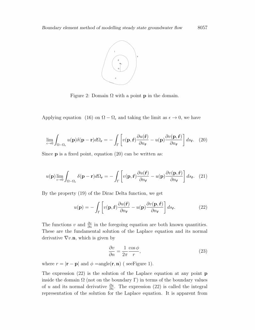
2.4 Integral equation for points on the boundary Γ

We study the general case where the boundary is not smooth and p is a corner

point where the fundamental solution v is singular. We consider the domain

Ω∗ which results from Ω after subtracting a small circular section with center

p, radius ε and confined by the arcs Ap and pB. The circular arc AB is

denoted Γε and the sum of the arcs Ap and pB by l. The outward normal to

Γε coincides with the radius ε and is directed towards the center p. The angle

between the tangents of the boundary at point p is denoted by α. Hence, it is

obvious that,

limε→ 0

(θ1 − θ2) = α, (24)

limε→ 0

Γε = 0, (25)

and

limε→ 0

(Γ− l) = Γ. (26)

r

t

A B

P

o

pq

c

x

+s

+s

a

b

k

n

Figure 3: Geometric definitions related to a corner point p of a non-smooth

boundary [4].

Next we apply Green’s identity in the domain Ω∗ for the functions u and v

satisfying equations (5) and (11) respectively. Since point p lies outside the


domain Ω∗, where δ(r− p) = 0, it follows that∫Ω∗u(p)δ(Q− P )dΩ = 0 (27)

and consequently Green’s identity generates

0 =

∫Γ−l

(v∂u

∂n− u∂v

∂n

)ds+

∫Γε

(v∂u

∂n− u∂v

∂n

)ds = I1 + I2. (28)

We will examine next the behavior of the integrals in the above equation when

ε→ 0. The integral I1 becomes

I1 = limε→0

∫Γ−l

(v∂u

∂n− u∂v

∂n

)ds =

∫Γ

(v∂u

∂n− u∂v

∂n

)ds. (29)

The integral I2 is written as

I2 =

∫Γε

(v∂u

∂n− u∂v

∂n

)ds =

∫Γε

1

2π

∂u

∂nln rds−

∫Γε

1

2πucosφ

rds = I1 + I2.

(30)

For the circular arc Γε, its r = ε and φ = π. Moreover, ds = ε(−dθ), because

the angle θ in the counter-clockwise sense, which is opposite to that of increas-

ing s. Therefore, the first of the resulting two integrals in equation (30), takes

the form

I1 =

∫Γε

1

2π

∂u

∂nln rds =

∫ θ2

θ1

1

2π

∂u

∂nε ln εd(−θ). (31)

By the mean value theorem of integral calculus, the value of the integral is

equal to the value of integrand at some point O within the integration interval

multiplied by the length of that interval. Hence,

I1 =1

2π

[∂u

∂n

]O

ε ln ε(θ1 − θ2). (32)

When ε → 0, the point O of the arc approaches point p. In this case, the

derivative[∂u∂n

]p, though not defined, it is bounded. Nevertheless, it is

limε→0

(ε ln ε) = 0

which implies that

limε→0

I1 = 0 (33)

In a similar way, the second integral I2 of equation (30) may be written as

I2 = −∫

Γε

1

2πucosφ

rds = −

∫ θ2

θ1

1

2πu−1

εεd(−θ) (34)


by applying the mean value theorem

I2 =−1

2πu0(θ2 − θ1) =

θ1 − θ2

2πu0 (35)

and finally, by condition (24)

limε→0

I2 =α

2πu(p). (36)

By virtue of equations (33) and (36), (30) yields

limε→0

∫Γε

[v∂u

∂n− u∂v

∂n

]ds =

α

2πu(p). (37)

Incorporating the findings of equations (29) and (37) into (28), the latter gives

for ε→ 0,

α

2πu(p) = −

∫Γ

[v(p, r)

∂u(r)

∂nr

− u(r)∂v(p, r)

∂nr

]dsr, (38)

which is the integral representation of the solution for the Laplace equation

at points p ∈ Γ, where the boundary is not smooth. For point p, where the

boundary is smooth, its α = π and thus, equation (38) becomes

1

2u(p) = −

∫Γ

[v(p, r)

∂u(r)

∂nr

− u(r)∂v(p, r)

∂nr

]dsr. (39)

A comparison between equations (22) and (38) reveals that the function u is

discontinuous when the point p ∈ Ω approaches point p ∈ Γ. It exhibits a

jump equal to (1 − α2π

) for corner points, or 12

for points on smooth parts of

the boundary Γ.

2.5 Integral equation for points outside the domain Ω

When the point p is located outside the domain Ω, Green,s identity gives

0 = −∫

Γ

[v(p, r)

∂u(r)

∂nr

− u(r)∂v(p, r)

∂nr

]dsr. (40)

Equations (22), (39) and (40) can be combined in a single general equation as

ε(p)u(p) = −∫

Γ

[v(p, r)

∂u(r)

∂nr

− u(r)∂v(p, r)

∂nr

]dsr, (41)


where ε(p) is a coefficient which depends on the position of point p [13] and

is defined as

ε(p) =

1 for p inside Ω,12

for p on a smooth boundary Γ,

0 for p outside Ω.

Equation (39) constitutes a compatibility relation between the boundary val-

ues of u and ∂u∂n

, meaning that only one of the quantities u and ∂u∂n

can be

prescribed at each point of the boundary. At the same time, equation (39)

can be viewed as an integral equation on the boundary Γ, that is, a bound-

ary integral equation with unknown as the quantity which is not prescribed

by the boundary condition. In the following development of BEM, we as-

sume a smooth boundary Γ. Thus, for the Dirichlet problem with u=u on Γ,

equation (39) is written as

1

2u = −

∫Γ

(v∂u

∂n− u∂v

∂n

)ds (42)

in which the only unknown is the function ∂u∂n

on Γ. For the Neumann problem,∂u∂n

= un, equation (39) becomes

1

2u = −

∫Γ

(vun − u

∂v

∂n

)ds (43)

with only the unknown as the function u on Γ. For problems with mixed

boundary conditions, equation (39) is treated as two separate equations,

namely

1

2u = −

∫Γ

(v∂u

∂n− u∂v

∂n

)ds on Γ1 (44)

and1

2u = −

∫Γ

(vun − u

∂u

∂n

)ds on Γ2. (45)

2.6 Undergroundwater Flow Model For the Present Study

The flow area is assumed rectangular with Neumann boundary conditions on

two sides and Dirichlet boundary conditions on the other two as shown by

Figure 4. We consider isotropic flow which leads to the Laplace equation.


a

b

ce t

d

f

g i

j

h

k l

m

Figure 4: Underground water flow model of the steady-state where t and k

can be constant or variable.

3 Implementation of BEM

We now show how equation (41) may be applied to obtain a simple boundary

element procedure for solving numerically the interior boundary value problem

defined by equations (6),(7) and (8). The advantage of the BEM is to discretize

the boundary into finite number of segments, not necessarily equal, which

are called boundary elements or elements. The usually employed boundary

elements are the constant elements, the linear elements and the parabolic or

quadratic elements [4]. On each element, we distinguish the extreme points

or end points and the nodes or nodal points. The latter are the points at

which values of the boundary quantities are assigned. In the case of constant

elements, the boundary segment is approximated by a straight line, which

connects its extreme points. The node is placed at the mid-point of the straight

line and the boundary quantity is assumed to be constant along the element

and equal to its value at the nodal point as shown in Figure 5 [12]. In this

work, the numerical solution of the integral equation (41) will be presented

using constant boundary elements.


3.1 The BEM with constant boundary elements

The boundary Γ is approximated as a union of elements. That is, ∪Nj=1Γj 'Γ. The values of the boundary quantity u and its normal derivative ∂u

∂nare

assumed constant over each element and equal to their value at the mid-point

of the element.

1

2

34

5

6

7 8

a b

c

d

ef

g

h

endnodes

element

Figure 5: Discretisation of a circle into elements Γi

The discretized form of equation (39) is expressed for a given point pi on Γ

as

1

2ui = −

N∑j=1

∫Γj

v(pi, r)∂u(r)

∂nr

dsr +N∑j=1

∫Γj

u(r)∂v(pi, r)

∂nr

dsr (46)

where Γj is the element on which j-th node is located and over which integration

is carried out, pi is the nodal point of the i-th element and and ui is the value of

the function u at the point pi. For constant elements, the boundary is smooth

at the nodal points, hence ε(p) = 12. The values of u and ∂u

∂ndenoted un can be

moved outside the integral since they are constant on each element. Denoting

u by uj and un by ujn on the j-th element, equation (46) may be written as

−1

2ui +

N∑j=1

(∫Γj

∂v

∂nds

)uj =

N∑j=1

(∫Γj

vds

)ujn. (47)

The values of the foregoing integrals express the contribution of the nodal

values uj and ujn to the formation of the value 12ui. For this reason,they are

often referred to as influence coefficients [4]. These coefficients are denoted


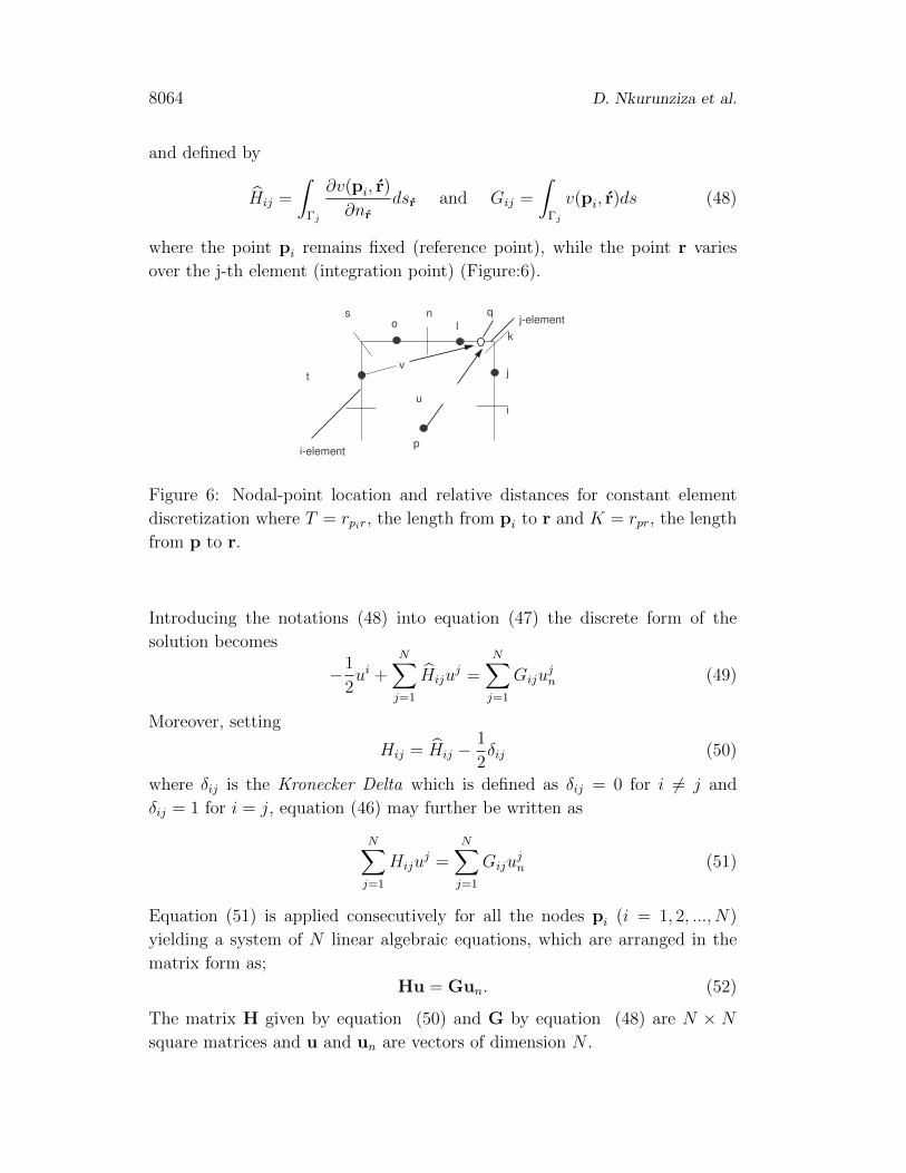
and defined by

Hij =

∫Γj

∂v(pi, r)

∂nr

dsr and Gij =

∫Γj

v(pi, r)ds (48)

where the point pi remains fixed (reference point), while the point r varies

over the j-th element (integration point) (Figure:6).

i

j

kl

no

s

t

p

u

j-element

i-element

v

q

Figure 6: Nodal-point location and relative distances for constant element

discretization where T = rpir, the length from pi to r and K = rpr, the length

from p to r.

Introducing the notations (48) into equation (47) the discrete form of the

solution becomes

−1

2ui +

N∑j=1

Hijuj =

N∑j=1

Gijujn (49)

Moreover, setting

Hij = Hij −1

2δij (50)

where δij is the Kronecker Delta which is defined as δij = 0 for i 6= j and

δij = 1 for i = j, equation (46) may further be written as

N∑j=1

Hijuj =

N∑j=1

Gijujn (51)

Equation (51) is applied consecutively for all the nodes pi (i = 1, 2, ..., N)

yielding a system of N linear algebraic equations, which are arranged in the

matrix form as;

Hu = Gun. (52)

The matrix H given by equation (50) and G by equation (48) are N × Nsquare matrices and u and un are vectors of dimension N .


Assuming mixed boundary conditions, in this case, the part Γ1 of the boundary

on which u is prescribed and the part Γ2 on which un is prescribed, are dis-

cretized intoN1 andN2 constant elements, respectively (Γ1∪Γ2 = Γ, N1+N2 =

N). Hence, equation (52) again contains N unknowns, that is N−N1 values of

u on Γ2 and N−N2 values of un on Γ1. These N unknowns may be determined

from the system of equations (52).

We have to separate the unknown from the known quantities when we solve

the system. By partitioning the matrices, equation (52) can be written as

[H11 H12]

u1

u2

= [G11 G12]

un1

un2

(53)

where u1 and un2 are the known quantities on Γ1 and Γ2 respectively,

while un1 and u2 denote the corresponding unknown ones. Taking all the

unknown to the left hand side of the equation and the known ones to the right

hand side, we obtained

Ax = b (54)

where

A = [H12 −G11] , (55)

x =

u2

un1

(56)

b = −H11 u1 +G12 un2 . (57)

A is an N ×N square matrix, and x, b vectors with dimensions N[12].

Matrices A and b can also be constructed using an alternative straightforward

procedure, which is based on the observation that matrix A will eventually

contain all the columns of H and G that correspond to the unknown boundary

values of u and un, whereas vector b will result as the sum of those columns of

H and G, which correspond to the known values u and un, after they have been

multiplied by these values. It should be noted that a change of sign occurs,

when the columns of G or H are moved to the other side of the equation [4].

The solution of the simultaneous equations (54) yield the unknown boundary

quantities u and un. Therefore, knowing all the boundary quantities on Γ, the

solution u can be computed at any point p(x, y) in the domain Ω by virtue of


equation (41) for ε(p) = 1. Applying the same discretization as in equation

(46), we arrived at the following expression

u(p) =N∑j=1

Hijuj −

N∑j=1

Gijujn. (58)

The coefficients Gij and Hij are computed again from the integrals (48), but

in this case the boundary point pi, is replaced in the expression by the field

point p in Ω ( see Figure 6).

The line integrals Gij and Hij defined in equation (48) are evaluated numeri-

cally using a standard Gaussian quadrature [6]. Of course,these integrals can

be evaluated numerically through symbolic languages, but the resulting expres-

sions are very lengthy. Hence the advantage of accuracy over the numerical

integration is rather lost, due to the complexity of the most suitable method

for computing line integrals. Two cases are distinguished for the integrals of

the influence coefficients:

(i) Off-diagonal elements, i 6= j: In this case, the point pi(xi, yi) lies outside

the j-element, which means that the distance r = |r−pi| does not vanish

and, consequently, the integral is regular.

The Gaussian integration is performed over the interval −1 ≤ ξ ≤ 1 as∫ 1

−1

f(ξ)dξ =n∑k=1

wkf(ξk) (59)

where n is the number of integration points (Gauss points), and ξk and wk(k = 1, 2, 3, ..., n) are the abscissas and weights of the Gaussian quadra-

ture of order n.

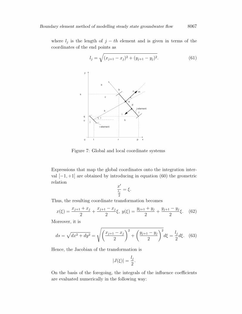
Let us consider the element j over which the integration will be carried

out. This elements is defined by the coordinates (xj, yj) and (xj+1, yj+1)

of its extreme points, which are expressed in a global system having axes

x and y, and origin at point O (see Figure: 7). Subsequently, a local

system of axes x′ and y′ is introduced at point pj of the element. The

local coordinates (x′, o) of point r on the j − th element are related to

the global coordinates of the xy-system through the expressions

x =xj+1 + xj

2+xj+1 − xj

ljx′, y =

yj+1 + yj2

+yj+1 − yj

ljx′, − lj

2≤ x′ ≤ lj

2(60)


where lj is the length of j − th element and is given in terms of the

coordinates of the end points as

lj =√

(xj+1 − xj)2 + (yj+1 − yj)2. (61)

a

bn

d

c

e

f

h

i

k

x

y

o

j-element

i-element

m

l

j

p

q

r

s

t

u

Figure 7: Global and local coordinate systems

Expressions that map the global coordinates onto the integration inter-

val [−1,+1] are obtained by introducing in equation (60) the geometric

relationx′

lj2

= ξ.

Thus, the resulting coordinate transformation becomes

x(ξ) =xj+1 + xj

2+xj+1 − xj

2ξ, y(ξ) =

yj+1 + yj2

+yj+1 − yj

2ξ. (62)

Moreover, it is

ds =√dx2 + dy2 =

√(xj+1 − xj

2

)2

+

(yj+1 − yj

2

)2

dξ =lj2dξ. (63)

Hence, the Jacobian of the transformation is

|J(ξ)| = lj2.

On the basis of the foregoing, the integrals of the influence coefficients

are evaluated numerically in the following way:


(a) The integral of Gij

Gij =

∫Γj

vds =

∫ 1

−1

1

2πln[r(ξ)]

lj2dξ =

lj4π

n∑k=1

ln[r(ξk)]wk (64)

where

r(ξk) =√

[x(ξk)− xi]2 + [y(ξk)− yi]2 (65)

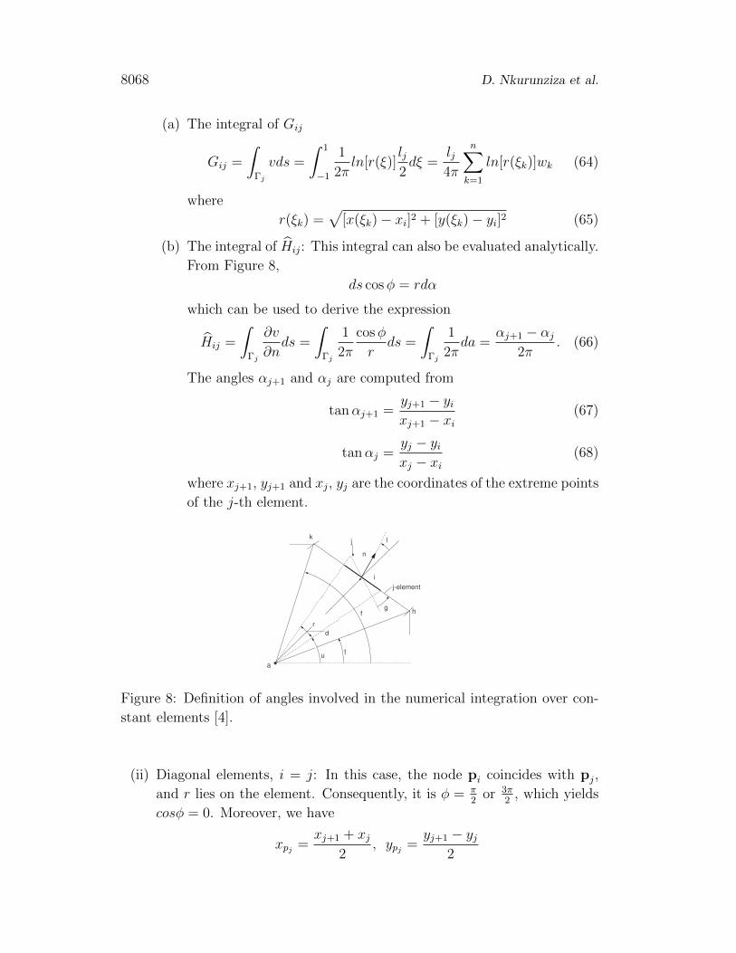
(b) The integral of Hij: This integral can also be evaluated analytically.

From Figure 8,

ds cosφ = rdα

which can be used to derive the expression

Hij =

∫Γj

∂v

∂nds =

∫Γj

1

2π

cosφ

rds =

∫Γj

1

2πda =

αj+1 − αj2π

. (66)

The angles αj+1 and αj are computed from

tanαj+1 =yj+1 − yixj+1 − xi

(67)

tanαj =yj − yixj − xi

(68)

where xj+1, yj+1 and xj, yj are the coordinates of the extreme points

of the j-th element.

a

d

r

fg

h

i

jk

n

j-element

tu

l

Figure 8: Definition of angles involved in the numerical integration over con-

stant elements [4].

(ii) Diagonal elements, i = j: In this case, the node pi coincides with pj,

and r lies on the element. Consequently, it is φ = π2

or 3π2

, which yields

cosφ = 0. Moreover, we have

xpj =xj+1 + xj

2, ypj =

yj+1 − yj2


and

r(ξ) =√

[x(ξ)− xpj ]2 + [y(ξ)− ypj ]2 =lj2|ξ|. (69)

Hence,

Gjj =

∫Γj

1

2πlnrds = 2

∫ lj2

0

1

2πlnrdr =

1

π[rlnr−r]lj/20 =

1

2

lj2

[ln(lj/2)−1],

(70)

and

Hjj =1

2π

∫Γj

cosφ

rds =

1

2π

∫ 1

−1

cosφ

|ξ|dξ =

2

2π[cosφ ln |ξ|]10 = 0. (71)

4 Results

In this section, we present results to the model in subsection 2.6. We considered

different cases of boundary conditions and obtained the hydraulic head at

chosen points in the domain.

4.1 Specified head and no flux at Neumann sides

This type of boundary conditions is known as no flow Boundary, it is a special

type of the prescribed flux boundary and is also referred to as no-flux, zero

flux, impermeable, reflective or barrier boundary. No flow boundaries are

impermeable boundaries that allow zero flux. They are physical or hydrological

barriers which inhibit the inflow or outflow of water in the model domain,

Figure 9. The expressions h1 and h2 are the values of the hydraulic head at

the boundary of the domain. A simulation of the model with these boundary

conditions produced the groundwater head distribution shown in Figure 10

and the direction of flow is shown in Figure 11.


a

b

c

d

e

Figure 9: Undergroundwater flow model of the steady-state with non flow

boundaries

0.1 0.2 0.3 0.4 0.5 0.6 0.7 0.8 0.90.1

0.2

0.3

0.4

0.5

0.6

0.7

0.8

0.9

55

60

65

70

75

80

85

90

95

Figure 10: Surface representation of h lev-

els when h1 = 100m, h2 = 50m, and dhdn

as

shown in Figure 9.

0.1 0.2 0.3 0.4 0.5 0.6 0.7 0.8 0.90

0.1

0.2

0.3

0.4

0.5

0.6

0.7

0.8

0.9

Figure 11: Gradient representation of the

flow for the model in Figure 9

4.2 Different flux values at Neumann sides

In Figure 12, we assume the model defined in Section 2.6 with the same

values of h1 and h2 at the boundary as in Figure 9 presented in Section 4.1.

We assume different values of the flux at Neumann sides as shown in Figure 12.

A simulation with these boundary conditions produced the groundwater head

distribution shown in Figure 13 and the direction of flow is shown in Figure

14.


a

b

c

d

e

Figure 12: Undergroundwater flow model of the steady-state with zero flux at

one of Neumann sides and non zero flux for another

0.1 0.2 0.3 0.4 0.5 0.6 0.7 0.8 0.90.1

0.2

0.3

0.4

0.5

0.6

0.7

0.8

0.9

55

60

65

70

75

80

85

90

95



as

shown in Figure 12

0.1 0.2 0.3 0.4 0.5 0.6 0.7 0.8 0.90

0.1

0.2

0.3

0.4

0.5

0.6

0.7

0.8

0.9


flow for the model in Figure 12.

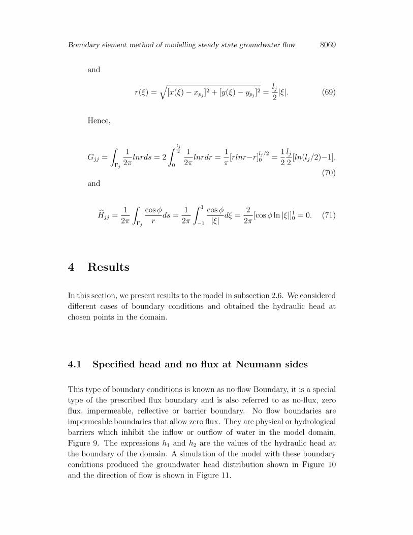
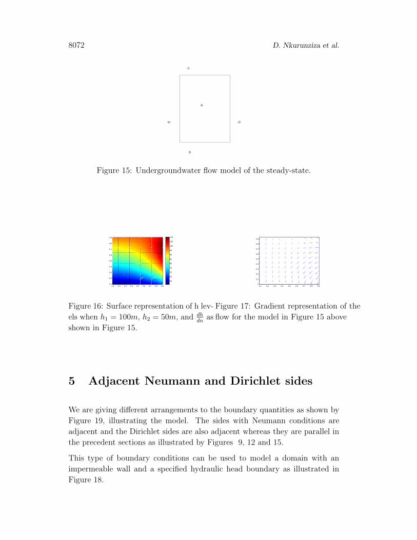
4.3 Mixed experimental boundary conditions

Now, let us assume some values of the flux at the boundary of the domain

bigger than the ones used in Sections 4.1, and 4.2. The values of the flux

at Neumann sides are assumed to be 0 and 100 as illustrated in Figure 15.

A simulation with these boundary conditions produced the groundwater head

distribution shown in Figure 16 and the direction of flow is shown in Figure

17.


a

b

c

d

e

Figure 15: Undergroundwater flow model of the steady-state.

0.1 0.2 0.3 0.4 0.5 0.6 0.7 0.8 0.90.1

0.2

0.3

0.4

0.5

0.6

0.7

0.8

0.9

60

65

70

75

80

85

90

95

100

105

110



as

shown in Figure 15.

0.1 0.2 0.3 0.4 0.5 0.6 0.7 0.8 0.90

0.1

0.2

0.3

0.4

0.5

0.6

0.7

0.8

0.9


flow for the model in Figure 15 above

5 Adjacent Neumann and Dirichlet sides

We are giving different arrangements to the boundary quantities as shown by

Figure 19, illustrating the model. The sides with Neumann conditions are

adjacent and the Dirichlet sides are also adjacent whereas they are parallel in

the precedent sections as illustrated by Figures 9, 12 and 15.

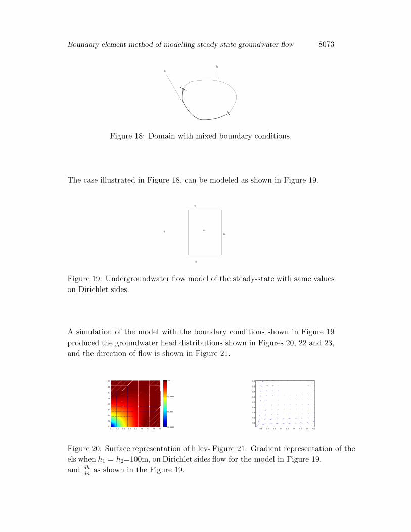
This type of boundary conditions can be used to model a domain with an

impermeable wall and a specified hydraulic head boundary as illustrated in

Figure 18.


b

a

Figure 18: Domain with mixed boundary conditions.

The case illustrated in Figure 18, can be modeled as shown in Figure 19.

a

b

c

de

Figure 19: Undergroundwater flow model of the steady-state with same values

on Dirichlet sides.

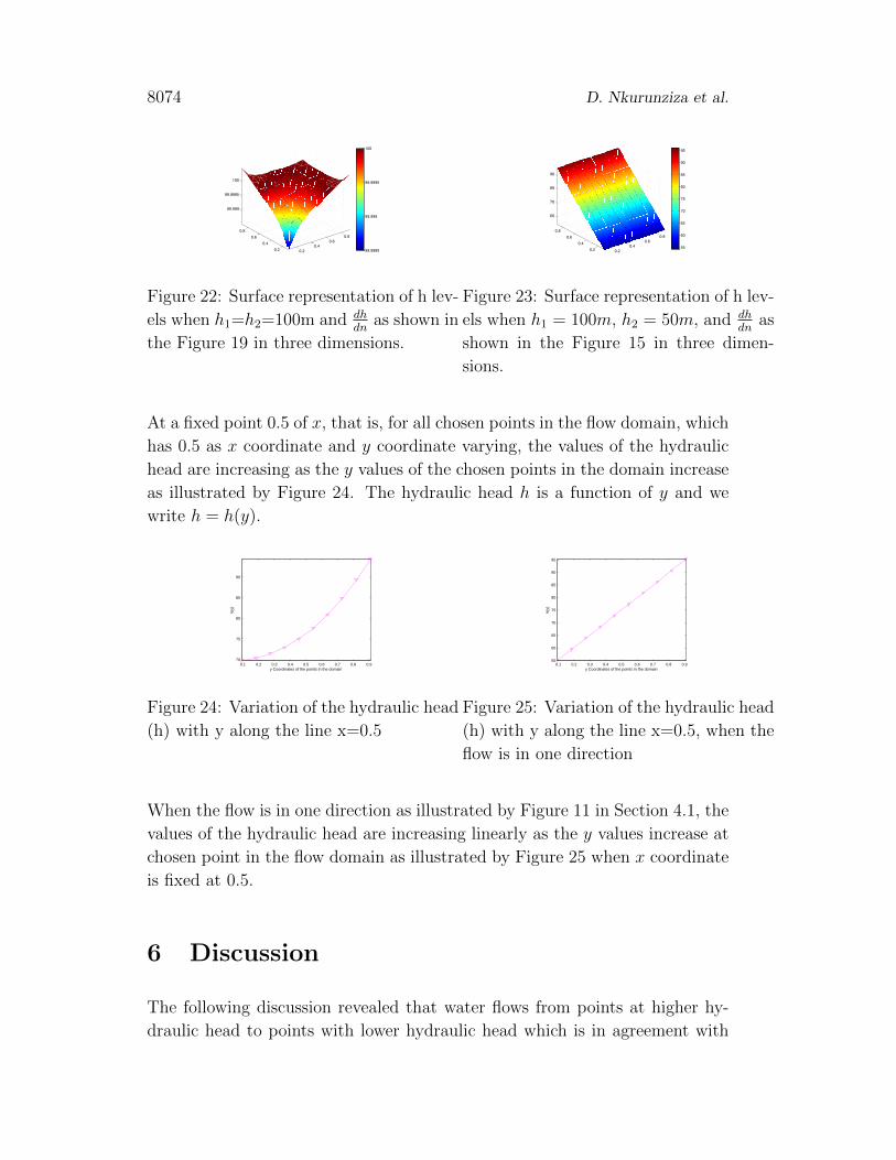
A simulation of the model with the boundary conditions shown in Figure 19

produced the groundwater head distributions shown in Figures 20, 22 and 23,

and the direction of flow is shown in Figure 21.

0.1 0.2 0.3 0.4 0.5 0.6 0.7 0.8 0.90.1

0.2

0.3

0.4

0.5

0.6

0.7

0.8

0.9

99.9985

99.999

99.9995

100


els when h1 = h2=100m, on Dirichlet sides

and dhdn

as shown in the Figure 19.

0.1 0.2 0.3 0.4 0.5 0.6 0.7 0.8 0.9

0.1

0.2

0.3

0.4

0.5

0.6

0.7

0.8

0.9


flow for the model in Figure 19.


0.2

0.4

0.6

0.8

0.2

0.4

0.6

0.8

99.999

99.9995

100

99.9985

99.999

99.9995

100


els when h1=h2=100m and dhdn

as shown in

the Figure 19 in three dimensions.

0.2

0.4

0.6

0.8

0.2

0.4

0.6

0.8

60

70

80

90

55

60

65

70

75

80

85

90

95



as

shown in the Figure 15 in three dimen-

sions.

At a fixed point 0.5 of x, that is, for all chosen points in the flow domain, which

has 0.5 as x coordinate and y coordinate varying, the values of the hydraulic

head are increasing as the y values of the chosen points in the domain increase

as illustrated by Figure 24. The hydraulic head h is a function of y and we

write h = h(y).

0.1 0.2 0.3 0.4 0.5 0.6 0.7 0.8 0.970

75

80

85

90

h(y)

y Coordinates of the points in the domain

Figure 24: Variation of the hydraulic head

(h) with y along the line x=0.5

0.1 0.2 0.3 0.4 0.5 0.6 0.7 0.8 0.955

60

65

70

75

80

85

90

95

h(y)

y Coordinates of the points in the domain

Figure 25: Variation of the hydraulic head

(h) with y along the line x=0.5, when the

flow is in one direction

When the flow is in one direction as illustrated by Figure 11 in Section 4.1, the

values of the hydraulic head are increasing linearly as the y values increase at

chosen point in the flow domain as illustrated by Figure 25 when x coordinate

is fixed at 0.5.

6 Discussion

The following discussion revealed that water flows from points at higher hy-

draulic head to points with lower hydraulic head which is in agreement with


the general theory of groundwater flow and also with the results obtained in

our 2014 paper [8].

The colorbar in Figure 10, show that values of the hydraulic head (h) in the

flow domain are varying from about 55 up to about 95 . The smallest value of

h in the flow domain is 54.8m at the points (5/11,1/11) and (6/11,1/11). The

highest value of h in the flow domain is 95.3m at the points (5/11,10/11) and

(6/11,10/11). By reducing the distance between the boundary of the domain

and the points in the flow domain, the smallest value of h can be very close

to 50m than 54.8m which is obtained by taking the values of h in the flow

domain at 1/11 from the boundary of the domain. The arrows in Figure 11

which represent the gradient vectors show that water is flowing in one direction,

from high values of h to the lowest ones. We can also conclude that the flux

is remaining the same as the flux is equal to zero at Neumann sides which is

making all the vectors in Figure 11 representing the gradient to have the same

magnitude.

We can say that the values of the flux used in Sections 4.1, 4.2 are too small and

do not have a significant influence to the results as expected mathematically.

Moreover, the values of the hydraulic head and the flux used in this section

reflect the reality according to the literature. Hence, we can take our model as

experimental which means that the values at the boundary are not necessarily

reflecting the reality at the field, by replacing the value 0.0023 of the flux in

Figure 12 which is reflecting the reality by 100, which is not used any where

in the surveyed literature. The experimental model help us to check the effect

of the flux on the result of the model.

The result of this experimental model represented by Figure 15 generated

55.9m as the smallest value of h and 110.8m. These values of the smallest and

biggest values of h are very different to the ones obtained in Section 4.2 which

have the same arrangement of boundary quantities. Hence, we can conclude

that the value of the flux at the boundary is has a significant influence on the

values of h in the flow domain. The flow direction illustrated by Figure 17, is

also different from the ones illustrated by Figures 11, 14. So, we can conclude

that the value of the flux at the boundary of the flow domain influence both

the flow direction and the values of h in the flow domain. Since the flow is

coming from out of the model domain which flow domain do not allow the

flow at the opposite side where the flux is zero, the quantity of water increases

in the flow domain and the value of the hydraulic head also increases up to

110.8m as a maximum value of the head in the flow domain.


Figure 20 illustrates the value of the hydraulic head at any point of the flow

domain. The smallest value of h is 99.9985 and the biggest one is 100.0005.

The surface representation of values of h at chosen points in the flow domain

are distributed on the interval [99.9985,100.005] which is a very small range.

The color representing values which are on the interval [99.9995,100] is mainly

represented on the Figure 20 which means that at many points in the flow

domain, the values of h are on that interval.

The same results represented in Figure 20 which is the surface representation

in two dimension, can be represented in three dimension by the Figure 22. We

can also represent the values of h in the flow domain in three dimension by

Figure 23, when the model is represented by Figure 15.

6.1 Conclusions

In this study, a mathematical model for underground water flow which in-

cludes the governing equation and boundary conditions have been formulated

and analyzed. The general objective was to develop a prediction tool for under-

ground water flow model using the boundary element method. Two scenarios

were considered (when the number of elements at the boundary is fifty six and

when it is twenty eight) and two cases in each scenario were considered for

generating results. The model was transformed in terms of elements at the

boundary of its domain . Since we considered the steady state flow, the fixed

boundary values of the head (h) at the boundary of the domain took different

values to check its influence on values of h at different points in the model

domain. The results confirm that water moved from points with high values

of h to points with lower values of h.

The limitation of the model considered here is that we assumed regular bound-

aries with artificial boundary cionditions, which may slightly deviate from re-

ality.

The concluded research leaves rich areas for further research in the direction

of solute transport models and a consideration of irregular boundaries with

experimental data.


Acknowledgement

The authors express their gratitude for the financial support from the Inter-

national Science Program (ISP) based at Uppsala University in Sweden.

References

[1] Chen, J., and Hong, H. Review of dual boundary element methods

with emphasis on hypersingular integrals and divergent series. Applied

Mechanics Reviews 52 (1999), 17–33.

[2] Hunter, P., and Pullan, A. Fem/bem notes. Departament of Engi-

neering Science. The University of Auckland, New Zealand (2001).

[3] Jim, T., and Peter, A. A structured approach for calibration of steady-

state ground water flow models. Ground water 34, 3 (May-June 1996),

444–450.

[4] Katsikadelis. Boundary elements: Theory and Applications. Elsevier,

2002.

[5] Khodadad, M., and Ardakani, M. D. Inclusion identification by

inverse application of boundary element method, genetic algorithm and

conjugate gradient method. American Journal of Applied Sciences 5, 9

(2008), 1158–1166.

[6] Kirkup, S., Yazdani, J., Mastorakis, N., Poulos, M., Mlade-

nov, V., Bojkovic, Z., Simian, D., Kartalopoulos, S., Va-

ronides, A., and Udriste, C. A gentle introduction to the boundary

element method in matlab/freemat. In WSEAS International Confer-

ence. Proceedings. Mathematics and Computers in Science and Engineer-

ing (2008), no. 10, WSEAS.

[7] Mango, J., and Kaahwa, Y. Error investigations in the interior laplace

problem using boundary elements. A.M.S.E Journal 72, 3 (2002), 39–45.

[8] Muyinda, N., Kakuba, G., and Mango, J. M. Finite volume method

of modelling transient groundwater flow. Journal of Mathematics and

Statistics 10, 1 (2014), 92–110.


[9] Salgado-Ibarra, E. A. Boundary element method (bem) and method

of fundamental solutions (mfs) for the boundary value problems of the

2-d laplace’s equation. Master’s thesis, University of Nevada, Las Vegas,

December 2011.

[10] Strickland, T., and Korleski, C. Technical guidance manual for

groundwater investigations. Tech. rep., Ohio Environmental Protection

Agency Division of Drinking and Ground Waters, P.O. Box 1049 50 West

Town Street Columbus, Ohio 43216-1049 Phone: 614-644-2752, November

2007.

[11] Wake, J. S. Groundwater surface water interaction modelling using vi-

sual modflow and gis. Master’s thesis, Universiteit Gent Vrije Universiteit

Brussel Belgium, june 2008.

[12] Zalewski, B. F. Uncertainties in the solutions to boundary element

method: An interval approach. PhD thesis, CASE WESTERN RESERVE

UNIVERSITY, August 2008.

[13] Zhu, T., Zhang, J.-D., and Atluri, S. A local boundary integral

equation (lbie) method in computational mechanics, and a meshless dis-

cretization approach. Computational Mechanics 21, 3 (1998), 223–235.

Received: September 25, 2014; Published: November 19, 2014

Documents

Boundary Element Method of Modelling Steady State ... · PDF fileBoundary element method of modelling steady state groundwater ow 8053 Equation (3) includes the storage term (S s @h