Embed Size (px)
Citation preview
BOUT++ Users Manual
B.Dudson, University of York
July 14, 2013
Contents
1 Introduction 11.1 License and terms of use . . . . . . . . . . . . . . . . . . . . . . . . . . . . . 2
2 Getting started 32.1 Obtaining BOUT++ . . . . . . . . . . . . . . . . . . . . . . . . . . . . . . . 42.2 Installing an MPI compiler . . . . . . . . . . . . . . . . . . . . . . . . . . . . 42.3 Installing libraries . . . . . . . . . . . . . . . . . . . . . . . . . . . . . . . . . 52.4 Configuring analysis routines . . . . . . . . . . . . . . . . . . . . . . . . . . . 82.5 Compiling BOUT++ . . . . . . . . . . . . . . . . . . . . . . . . . . . . . . . 92.6 Running the test suite . . . . . . . . . . . . . . . . . . . . . . . . . . . . . . 10
3 Advanced installation options 103.1 File formats . . . . . . . . . . . . . . . . . . . . . . . . . . . . . . . . . . . . 103.2 SUNDIALS . . . . . . . . . . . . . . . . . . . . . . . . . . . . . . . . . . . . 113.3 PETSc . . . . . . . . . . . . . . . . . . . . . . . . . . . . . . . . . . . . . . . 123.4 LAPACK . . . . . . . . . . . . . . . . . . . . . . . . . . . . . . . . . . . . . 133.5 MUMPS . . . . . . . . . . . . . . . . . . . . . . . . . . . . . . . . . . . . . . 133.6 MPI compilers . . . . . . . . . . . . . . . . . . . . . . . . . . . . . . . . . . . 143.7 Issues . . . . . . . . . . . . . . . . . . . . . . . . . . . . . . . . . . . . . . . 14
3.7.1 Wrong install script . . . . . . . . . . . . . . . . . . . . . . . . . . . . 143.7.2 Compiling cvode.cxx fails . . . . . . . . . . . . . . . . . . . . . . . . 14
4 Running BOUT++ 154.1 When things go wrong . . . . . . . . . . . . . . . . . . . . . . . . . . . . . . 184.2 Startup output . . . . . . . . . . . . . . . . . . . . . . . . . . . . . . . . . . 184.3 Per-timestep output . . . . . . . . . . . . . . . . . . . . . . . . . . . . . . . 24
1

CONTENTS 2
5 Output and post-processing 245.1 Note on reading PDB files . . . . . . . . . . . . . . . . . . . . . . . . . . . . 255.2 Reading BOUT++ output into IDL . . . . . . . . . . . . . . . . . . . . . . . 255.3 Summary of IDL file routines . . . . . . . . . . . . . . . . . . . . . . . . . . 275.4 IDL analysis routines . . . . . . . . . . . . . . . . . . . . . . . . . . . . . . . 285.5 Python routines . . . . . . . . . . . . . . . . . . . . . . . . . . . . . . . . . . 295.6 Matlab routines . . . . . . . . . . . . . . . . . . . . . . . . . . . . . . . . . . 305.7 Mathematica routines . . . . . . . . . . . . . . . . . . . . . . . . . . . . . . . 305.8 Octave routines . . . . . . . . . . . . . . . . . . . . . . . . . . . . . . . . . . 31
6 BOUT++ options 316.1 Command line options . . . . . . . . . . . . . . . . . . . . . . . . . . . . . . 326.2 General options . . . . . . . . . . . . . . . . . . . . . . . . . . . . . . . . . . 326.3 Time integration solver . . . . . . . . . . . . . . . . . . . . . . . . . . . . . . 346.4 Input and Output . . . . . . . . . . . . . . . . . . . . . . . . . . . . . . . . . 346.5 Laplacian inversion . . . . . . . . . . . . . . . . . . . . . . . . . . . . . . . . 366.6 Communications . . . . . . . . . . . . . . . . . . . . . . . . . . . . . . . . . 366.7 Differencing methods . . . . . . . . . . . . . . . . . . . . . . . . . . . . . . . 366.8 Model-specific options . . . . . . . . . . . . . . . . . . . . . . . . . . . . . . 376.9 Variable initialisation . . . . . . . . . . . . . . . . . . . . . . . . . . . . . . . 37
6.9.1 Original method . . . . . . . . . . . . . . . . . . . . . . . . . . . . . 376.9.2 Expressions . . . . . . . . . . . . . . . . . . . . . . . . . . . . . . . . 38
6.10 Boundary conditions . . . . . . . . . . . . . . . . . . . . . . . . . . . . . . . 406.10.1 Relaxing boundaries . . . . . . . . . . . . . . . . . . . . . . . . . . . 426.10.2 Shifted boundaries . . . . . . . . . . . . . . . . . . . . . . . . . . . . 426.10.3 Changing the width of boundaries . . . . . . . . . . . . . . . . . . . . 436.10.4 Examples . . . . . . . . . . . . . . . . . . . . . . . . . . . . . . . . . 43
7 Generating input grids 447.1 From EFIT files . . . . . . . . . . . . . . . . . . . . . . . . . . . . . . . . . . 457.2 From ELITE and GATO files . . . . . . . . . . . . . . . . . . . . . . . . . . 477.3 Generating equilibria . . . . . . . . . . . . . . . . . . . . . . . . . . . . . . . 477.4 Running pdb2bout . . . . . . . . . . . . . . . . . . . . . . . . . . . . . . . . 47
8 Fluid equations 518.1 Variables . . . . . . . . . . . . . . . . . . . . . . . . . . . . . . . . . . . . . . 528.2 Evolution equations . . . . . . . . . . . . . . . . . . . . . . . . . . . . . . . . 538.3 Input options . . . . . . . . . . . . . . . . . . . . . . . . . . . . . . . . . . . 548.4 Communication . . . . . . . . . . . . . . . . . . . . . . . . . . . . . . . . . . 558.5 Boundary conditions . . . . . . . . . . . . . . . . . . . . . . . . . . . . . . . 57

CONTENTS 3
8.5.1 Custom boundary conditions . . . . . . . . . . . . . . . . . . . . . . . 588.6 Initial profiles . . . . . . . . . . . . . . . . . . . . . . . . . . . . . . . . . . . 608.7 Output variables . . . . . . . . . . . . . . . . . . . . . . . . . . . . . . . . . 61
9 Fluid equations 2: reduced MHD 619.1 Printing messages/warnings . . . . . . . . . . . . . . . . . . . . . . . . . . . 639.2 Laplacian inversion . . . . . . . . . . . . . . . . . . . . . . . . . . . . . . . . 639.3 Error handling . . . . . . . . . . . . . . . . . . . . . . . . . . . . . . . . . . 65
10 Object-orientated interface 66
11 Differential operators 6711.1 Differencing methods . . . . . . . . . . . . . . . . . . . . . . . . . . . . . . . 6811.2 Non-uniform meshes . . . . . . . . . . . . . . . . . . . . . . . . . . . . . . . 6911.3 Operators . . . . . . . . . . . . . . . . . . . . . . . . . . . . . . . . . . . . . 7011.4 Setting differencing method . . . . . . . . . . . . . . . . . . . . . . . . . . . 71
12 Staggered grids 71
13 Advanced methods 7313.1 Preconditioning . . . . . . . . . . . . . . . . . . . . . . . . . . . . . . . . . . 7313.2 Jacobian function . . . . . . . . . . . . . . . . . . . . . . . . . . . . . . . . . 7713.3 DAE constraint equations . . . . . . . . . . . . . . . . . . . . . . . . . . . . 7713.4 Monitoring the simulation output . . . . . . . . . . . . . . . . . . . . . . . . 77
14 Examples 7814.1 advect1d . . . . . . . . . . . . . . . . . . . . . . . . . . . . . . . . . . . . . . 7814.2 drift-instability . . . . . . . . . . . . . . . . . . . . . . . . . . . . . . . . . . 7814.3 em-drift . . . . . . . . . . . . . . . . . . . . . . . . . . . . . . . . . . . . . . 7914.4 gyro-gem . . . . . . . . . . . . . . . . . . . . . . . . . . . . . . . . . . . . . . 7914.5 interchange-instability . . . . . . . . . . . . . . . . . . . . . . . . . . . . . . 7914.6 jorek-compare . . . . . . . . . . . . . . . . . . . . . . . . . . . . . . . . . . . 7914.7 lapd-drift . . . . . . . . . . . . . . . . . . . . . . . . . . . . . . . . . . . . . 7914.8 orszag-tang . . . . . . . . . . . . . . . . . . . . . . . . . . . . . . . . . . . . 7914.9 shear-alfven-wave . . . . . . . . . . . . . . . . . . . . . . . . . . . . . . . . . 8014.10sod-shock . . . . . . . . . . . . . . . . . . . . . . . . . . . . . . . . . . . . . 8014.11uedge-benchmark . . . . . . . . . . . . . . . . . . . . . . . . . . . . . . . . . 80

1. Introduction 4
15 Notes 8015.1 Compile options . . . . . . . . . . . . . . . . . . . . . . . . . . . . . . . . . . 8015.2 Adaptive grids . . . . . . . . . . . . . . . . . . . . . . . . . . . . . . . . . . . 80
15.2.1 Moving meshes . . . . . . . . . . . . . . . . . . . . . . . . . . . . . . 8015.2.2 Changing resolution . . . . . . . . . . . . . . . . . . . . . . . . . . . 81
A Installing PACT 81A.1 Self-extracting package . . . . . . . . . . . . . . . . . . . . . . . . . . . . . . 81A.2 PACT source distribution . . . . . . . . . . . . . . . . . . . . . . . . . . . . 81
B Compiling and running under AIX 83B.1 SUNDIALS . . . . . . . . . . . . . . . . . . . . . . . . . . . . . . . . . . . . 83
C BOUT++ functions (alphabetical) 85
D IDL routines 87
E Python routines (alphabetical) 93E.1 boututils . . . . . . . . . . . . . . . . . . . . . . . . . . . . . . . . . . . . . . 93E.2 boutdata . . . . . . . . . . . . . . . . . . . . . . . . . . . . . . . . . . . . . . 94
1 Introduction
BOUT++ is a C++ framework for writing plasma fluid simulations with an arbitrarynumber of equations in 3D curvilinear coordinates [?, ?]. It has been developed from theoriginal BOUndary Turbulence 3D 2-fluid edge simulation code [?, ?, ?] written by X.Xuand M.Umansky at LLNL.
Though designed to simulate tokamak edge plasmas, the methods used are very generaland almost any metric tensor can be specified, allowing the code to be used to simulate (forexample) plasmas in slab, sheared slab, and cylindrical coordinates. The restrictions on thesimulation domain are that the equilibrium must be axisymmetric (in the z coordinate),and that the parallelisation is done in the x and y (parallel to B) directions.
The aim of BOUT++ is to automate the common tasks needed for simulation codes, andto separate the complicated (and error-prone) details such as differential geometry, parallelcommunication, and file input/output from the user-specified equations to be solved. Thusthe equations being solved are made clear, and can be easily changed with only minimalknowledge of the inner workings of the code. As far as possible, this allows the user to con-centrate on the physics, rather than worrying about the numerics. This doesn’t mean thatusers don’t have to think about numerical methods, and so selecting differencing schemesand boundary conditions is discussed in this manual. The generality of the BOUT++ of

1.1 License and terms of use 5
course also comes with a limitation: although there is a large class of problems which can betackled by this code, there are many more problems which require a more specialised solverand which BOUT++ will not be able to handle. Hopefully this manual will enable you totest whether BOUT++ is suitable for your problem as quickly and painlessly as possible.
This manual is written for the user who wants to run (or modify) existing plasma models,or specify a new problem (grid and equations) to be solved. In either case, it’s assumed thatthe user isn’t all that interested in the details of the code. For a more detailed descriptionsof the code internals, see the developer and reference quides. After describing how to installBOUT++ (section 2), run the test suite (section 2.6) and a few examples (section 4, moredetail in section 14), increasingly sophisticated ways to modify the problem being solved areintroduced. The simplest way to modify a simulation case is by altering the input options,described in section 6. Checking that the options are doing what you think they should beby looking at the output logs is described in section 4, and an overview of the IDL analysisroutines for data post-processing and visualisation is given in section 5. Generating newgrid files, particularly for tokamak equilibria, is described in section 7.
Up to this point, little programming experience has been assumed, but performing moredrastic alterations to the physics model requires modifying C++ code. Section 8 describeshow to write a new physics model specifying the equations to be solved, using ideal MHDas an example. The remaining sections describe in more detail aspects of using BOUT++:section 11 describes the differential operators and methods available; section 12 covers theexperimental staggered grid system.
Various sources of documentation are:
� Most directories in the BOUT++ distribution contain a README file. This shoulddescribe briefly what the contents of the directory are and how to use them.
� This user’s manual, which goes through BOUT++ from a user’s point of view
� The developer’s manual, which gives details of the internal working of the code.
� The reference guide, which summarises functions, settings etc. Intended more forquick reference rather than a guide.
� Most of the code contains Doxygen comment tags (which are slowly getting bet-ter). Running doxygen (www.doxygen.org) on these files should therefore generate anHTML reference. This is probably going to be the most up-to-date documentation.
1.1 License and terms of use
Copyright 2010 B.D.Dudson, S.Farley, M.V.Umansky, X.Q.Xu
2. Getting started 6
BOUT++ is free software: you can redistribute it and/or modify
it under the terms of the GNU Lesser General Public License as published by
the Free Software Foundation, either version 3 of the License, or
(at your option) any later version.
BOUT++ is distributed in the hope that it will be useful,
but WITHOUT ANY WARRANTY; without even the implied warranty of
MERCHANTABILITY or FITNESS FOR A PARTICULAR PURPOSE. See the
GNU Lesser General Public License for more details.
You should have received a copy of the GNU Lesser General Public License
along with BOUT++. If not, see <http://www.gnu.org/licenses/>.
A copy of the LGPL license is in COPYING.LESSER. Since this is based
on (and refers to) the GPL, this is included in COPYING.
BOUT++ is free software, but since it is a scientific code we also ask that you showprofessional courtesy when using this code:
1. Since you are benefiting from work on BOUT++, we ask that you submit any im-provements you make to the code to us by emailing Ben Dudson at [email protected]
2. If you use BOUT++ results in a paper or professional publication, we ask that yousend your results to one of the BOUT++ authors first so that we can check them. Itis understood that in most cases if one or more of the BOUT++ team are involved inpreparing results then they should appear as co-authors.
3. Publications or figures made with the BOUT++ code should acknowledge the BOUT++code by citing B.Dudson et. al. Comp.Phys.Comm 2009 [?] and/or other BOUT++papers. See the file CITATION for details.
2 Getting started
This section goes through the process of getting, installing, and starting to run BOUT++.Only the basic functionality needed to use BOUT++ is described here; the next section (3)goes through more advanced options, and how to fix some common problems. This sectionwill go through the following steps:
1. Obtaining a copy of BOUT++
2. Installing an MPI compiler (2.2)

2.1 Obtaining BOUT++ 7
3. Installing libraries (2.3)
4. Configuring BOUT++ analysis codes (2.4)
5. Compiling BOUT++ (2.5)
6. Running the test suite (2.6)
Note: In this manual commands to run in a BASH shell will begin with ’$’, and com-mands specific to CSH with a ’%’.
2.1 Obtaining BOUT++
BOUT++ is now hosted publicly on github (http://github.com/bendudson/BOUT), andincludes instructions on downloading and installing BOUT++ in wiki pages. This websitealso has a list of current issues and history of changes. To obtain a copy of the latest version,run
$ git clone git://github.com/bendudson/BOUT.git
which will create a directory BOUT containing the code. To get the latest changes later, gointo the BOUT directory and run
$ git pull
For more details on using git to work with BOUT++, see the developer’s manual.
2.2 Installing an MPI compiler
To compile and run the examples BOUT++ needs an MPI compiler. If you are installingon a cluster or supercomputer then the MPI C++ compilers will already be installed, andon Cray or IBM machines will probably be called ’CC’ and ’xlC’ respectively. If you’reinstalling on a smaller server or your own machine then you need to check that you have anMPI compiler by running
$ mpicc
This should produce an error message along the lines of “no input files”, but if yousee something like “command not found” then you need to install MPI first. There areseveral free MPI distributions available, the main ones currently being MPICH2 (www.mcs.anl.gov/mpi/mpich2), OpenMPI (www.open-mpi.org/), and LAM (www.lam-mpi.org/).On Ubuntu or Debian distributions if you have administrator rights then you can installMPICH2 by running
2.2 Installing an MPI compiler 8
$ sudo apt-get install mpich2 libmpich2-dev
If this works, and you now have a working mpicc command, skip to the next sectionon installing libraries. If not, and particularly if you don’t have administrator rights, youshould install MPI in your home directory by compiling it from source. In your homedirectory, create two subdirectories: One called “install” where we’ll put the source code,and one called “local” where we’ll install the MPI compiler:
$ cd
$ mkdir install
$ mkdir local
Download the latest stable version of MPICH2 from http://www.mcs.anl.gov/research/
projects/mpich2/downloads/ and put the file in the “install” subdirectory created above.At the time of writing (June 2012), the file was called mpich2-1.4.1p1.tar.gz. Untar thefile:
$ tar -xzvf mpich2-1.4.1p1.tar.gz
which will create a directory containing the source code. ’cd’ into this directory and run
$ ./configure --prefix=$HOME/local
$ make
$ make install
Each of which might take a while. This is the standard way of installing software fromsource, and will also be used for installing libraries later. The --prefix= option specifieswhere the software should be installed. Since we don’t have permission to write in thesystem directories (e.g. /usr/bin), we just use a subdirectory of our home directory. Theconfigure command configures the install, finding the libraries and commands it needs.make compiles everything using the options found by configure. The final make install
step copies the compiled code into the correct places under $HOME/local.To be able to use the MPI compiler, you need to modify the PATH environment variable.
To do this, run
$ export PATH=$PATH:$HOME/local/bin
and add this to the end of your startup file $HOME/.bashrc. If you’re using CSH ratherthan BASH, the command is
% setenv PATH ${PATH}:${HOME}/local/bin
and the startup file is $HOME/.cshrc. You should now be able to run mpicc and so have aworking MPI compiler.

2.3 Installing libraries 9
2.3 Installing libraries
After getting an MPI compiler, the next step is to make sure the libraries BOUT++ needsare installed. At minimum BOUT++ needs the FFTW-3 library, and to run any of theexamples you’ll also need NetCDF-4 (prior to 4.2) installed.
NOTE: There are currently issues with support for NetCDF’s new C++ API,which appeared in 4.2. For now use NetCDF 4.1.x
Most large machines (e.g. NERSC Hopper, HECToR, HPC-FF etc.) will have theselibraries and many more already installed, but you may need to load a module to use them.To see a list of the available modules, try running
modules avail
which works on many systems, but not all. See your system’s documentation on modulesand which ones to load. If you don’t know, or modules don’t work, you can still installlibraries in your home directory by following the instructions below.
If you’re installing on your own machine, then install the packages for your distribution.On Ubuntu or Debian, the necessary packages can be installed by running
$ sudo apt-get install libfftw3-dev libnetcdf-dev
The easiest way to test if the libraries are installed correctly is try configuring BOUT++.In the BOUT directory obtained previously, run
$ ./configure
If this finishes by printing a summary, and paths for IDL, Python, and Octave, then thelibraries are set up and you can skip to the next section. If you see a message “ERROR: FFTW
not found. Required by BOUT++” then you need to install FFTW-3. If you haven’talready, create directories “install” and “local” in your home directory:
$ cd
$ mkdir install
$ mkdir local
Download the latest stable version from http://www.fftw.org/download.html into the“install” directory. At the time of writing, this was called fftw-3.3.2.tar.gz. Untar thisfile, and ’cd’ into the resulting directory. As with the MPI compiler, configure and installthe FFTW library into $HOME/local by running:
$ ./configure --prefix=$HOME/local
$ make
$ make install

2.3 Installing libraries 10
Go back to the BOUT directory and re-run the configure script. If you used $HOME/local
as the prefix, BOUT++ configure should find the FFTW library now. If you installedsomewhere else, you can specify the directory with the --with-fftw= option:
$ ./configure --with-fftw=$HOME/local
Configure should now find FFTW, and search for the NetCDF library. If configurefinishes successfully, then skip to the next section, but if you see a message NetCDF support
disabled then configure couldn’t find the NetCDF library. Unless you have PACT orpnetcdf installed, this will be followed by a message ERROR: At least one file format
must be supported.Download the 4.1.3 bundled1 release of NetCDF from http://www.unidata.ucar.
edu/downloads/netcdf/netcdf-4_1_3/ and put the netcdf-4.1.3.tar.gz file into your“install” directory. Untar the file and ’cd’ into the resulting directory:
$ tar -xzvf netcdf-4.1.3.tar.gz
$ cd netcdf-4.1.3
As with MPI compilers and FFTW, configure, then make and make install:
$ ./configure --prefix=$HOME/local
$ make
$ make install
Sometimes configure can fail, in which case try disabling fortran and the HDF5 interface:
$ ./configure --prefix=$HOME/local --disable-fortran --disable-netcdf-4
$ make
$ make install
Go back to the BOUT directory and run the configure script again, this time specifyingboth the location of FFTW (if you installed it from source above), and the NetCDF library:
$ ./configure --with-fftw=$HOME/local --with-netcdf=$HOME/local
which should now finish successfully, printing a summary of the configuration:
Configuration summary
FACETS support: no
PETSc support: no
IDA support: no
CVODE support: no
1Support for the more recent unbundled versions is coming soon
2.4 Configuring analysis routines 11
NetCDF support: yes
Parallel-NetCDF support: no
PDB support: no
Hypre support: no
MUMPS support: no
If not, see section 3 for some things you can try to resolve common problems.
2.4 Configuring analysis routines
The BOUT++ installation comes with a set of useful routines which can be used to prepareinputs and analyse outputs. Most of this code is in IDL, but an increasing amount is inPython. In particular all the test suite scripts use Python, so to run these you’ll need thisconfigured. If you just want to compile BOUT++ then you can skip to the next section,but make a note of what configure printed out.
When the configure script finishes, it prints out the paths you need to get IDL, Python,and Octave analysis routines working. After running the command which looks like
$ export IDL_PATH=...
check that idl can find the analysis routines by running:
$ idl
IDL> .r collect
IDL> help, /source
You should see the function COLLECT in the BOUT/tools/idllib directory. If not, somethingis wrong with your IDL PATH variable. On some machines, modifying IDL PATH causesproblems, in which case you can try modifying the path inside IDL by running
IDL> !path = !path + ":/path/to/BOUT/tools/idllib"
where you should use the full path. You can get this by going to the tools/idllib directoryand typing ’pwd’. Once this is done you should be able to use collect and other routines.
To use Python, you will need the NumPy and SciPy libraries. On Debian or Ubuntuthese can be installed with
$ sudo apt-get install python-scipy
which should then add all the other dependencies like NumPy. To test if everything isinstalled, run
$ python
>>> import scipy
2.5 Compiling BOUT++ 12
If not, see the SciPy website http://www.scipy.org for instructions on installing.To do this, the path to tools/pylib should be added to the PYTHONPATH environment
variable. Instructions for doing this are printed at the end of the configure script, forexample:
Make sure that the tools/pylib directory is in your PYTHONPATH
e.g. by adding to your ~/.bashrc file
export PYTHONPATH=/home/ben/BOUT/tools/pylib/:$PYTHONPATH
To test if this command has worked, try running
$ python
>>> import boutdata
If this doesn’t produce any error messages then Python is configured correctly.
2.5 Compiling BOUT++
Once BOUT++ has been configured, you can compile the bulk of the code by going to theBOUT directory (same as configure) and running
$ make
(on OS-X, FreeBSD, and AIX this should be gmake). This should print something like:
----- Compiling BOUT++ -----
CXX = mpicxx
CFLAGS = -O -DCHECK=2 -DSIGHANDLE \
-DREVISION=13571f760cec446d907e1bbeb1d7a3b1c6e0212a \
-DNCDF -DBOUT_HAS_PVODE
CHECKSUM = ff3fb702b13acc092613cfce3869b875
INCLUDE = -I../include
Compiling field.cxx
Compiling field2d.cxx
At the end of this, you should see a file libbout++.a in the lib/ subdirectory of theBOUT++ distribution. If you get an error, please send an error report to a BOUT++developer such as mailto:[email protected] containing
� Which machine you’re compiling on
� The output from make, including full error message
� The make.config file in the BOUT++ root directory

2.6 Running the test suite 13
2.6 Running the test suite
In the examples/ subdirectory there are a set of short test cases which are intended totest portions of the BOUT++ code and catch any bugs which could be introduced. Torun the test cases, the Python libraries must first be set up by following the instructions insection 2.4. Go into the examples subdirectory and run
$ ./test_suite
This will go through a set of tests, each on a variety of different processors. Note:currently this uses the mpirun command to launch the runs, so won’t work on machineswhich use a job submission system like PBS or SGE.
These tests should all pass, but if not please send an error report to mailto:benjamin.
[email protected] containing
� Which machine you’re running on
� The make.config file in the BOUT++ root directory
� The run.log.* files in the directory of the test which failed
If the tests pass, congratulations! You have now got a working installation of BOUT++.Unless you want to use some experimental features of BOUT++, skip to section 4 to startrunning the code.
3 Advanced installation options
This section describes some common issues encountered when configuring and compilingBOUT++, and how to configure optional libraries like SUNDIALS and PETSc.
3.1 File formats
BOUT++ can currently use three different file formats: Portable Data Binary (PDB) whichis part of PACT2, NetCDF-43, and experimental support for Parallel NetCDF. PDB wasdeveloped at LLNL, was used in the UEDGE and BOUT codes, and was the original for-mat used by BOUT++. NetCDF is a more widely used format and so has many moretools for viewing and manipulating files. In particular, the NetCDF-4 library can producefiles in either NetCDF3 “classic” format, which is backwards-compatible with NetCDF li-braries since 1994 (version 2.3), or in the newer NetCDF4 format, which is based on (and
2http://pact.llnl.gov3http://www.unidata.ucar.edu/software/netcdf/
3.2 SUNDIALS 14
compatible with) HDF5. If you have both libraries installed then BOUT++ can use bothsimultaneously, for example reading in grid files in PDB format, but writing output data inNetCDF format.
To enable NetCDF support, you will need to install NetCDF version 4.0.1 or later. Notethat although the NetCDF-4 library is used for the C++ interface, by default BOUT++writes the “classic” format. Because of this, you don’t need to install zlib or HDF5 forBOUT++ NetCDF support to work. If you want to output to HDF5 then you need tofirst install the zlib and HDF5 libraries, and then compile NetCDF with HDF5 support.When NetCDF is installed, a script nc-config should be put into somewhere on the path.If this is found then configure should have all the settings it needs. If this isn’t found thenconfigure will search for the NetCDF include and library files.
PACT http://pact.llnl.gov/ is needed for reading and writing Portable Data Binary(PDB) format files. This is mainly for backwards compatibility with BOUT and UEDGE,and NetCDF-4 is recommended. If you need to be able to read or write PDB files, detailson installing PACT are given in Appendix A.
3.2 SUNDIALS
The BOUT++ distribution includes a 1998 version of CVODE (then called PVODE) byScott D. Cohen and Alan C. Hindmarsh, which is the default time integration solver. Whilstno serious bugs have been found in this code (as far as I am aware), several features suchas user-supplied preconditioners and constraints cannot be used with this solver. Currently,BOUT++ also supports the SUNDIALS solvers CVODE and IDA, which are available fromhttps://computation.llnl.gov/casc/sundials/main.html.
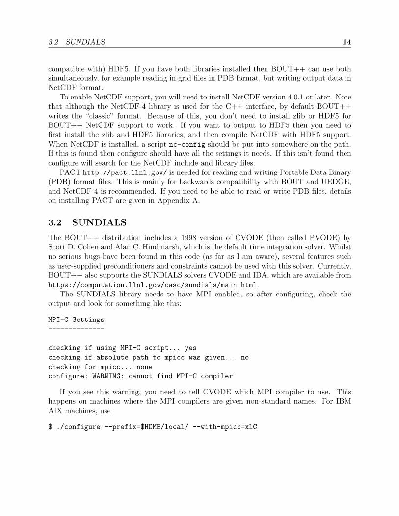
The SUNDIALS library needs to have MPI enabled, so after configuring, check theoutput and look for something like this:
MPI-C Settings
--------------
checking if using MPI-C script... yes
checking if absolute path to mpicc was given... no
checking for mpicc... none
configure: WARNING: cannot find MPI-C compiler
If you see this warning, you need to tell CVODE which MPI compiler to use. Thishappens on machines where the MPI compilers are given non-standard names. For IBMAIX machines, use
$ ./configure --prefix=$HOME/local/ --with-mpicc=xlC
3.3 PETSc 15
On NERSC’s Franklin, SUNDIALS needs to be compiled with “–with-mpicc=cc” to forceit to build the parallel libraries
The modern SUNDIALS CVODE solver is essentially the same as the 1998 CVODE(with some tweaking, re-arranging etc.), but this solver allows users to supply their ownpreconditioner and Jacobian functions. To use this solver, use
./configure --with-cvode
or
./configure --with-cvode=/path/to/cvode/
if your CVODE library is in a non-standard place.The SUNDIALS IDA solver is a Differential-Algebraic Equation (DAE) solver, which
evolves a system of the form f (u, u̇, t) = 0. This allows algebraic constraints on variablesto be specified. If you want this functionality, compile in the IDA library using
./configure --with-ida
or
./configure --with-ida=/path/to/ida/
You can compile in several of these libraries, for example
./configure --with-cvode --with-ida
is valid. This will allow you to select at run-time which solver to use. See section 6.3 formore details on how to do this.
3.3 PETSc
BOUT++ can use PETSc for time-integration and for solving elliptic problems, such asinverting Poisson and Helmholtz equations.
./configure --with-petsc
The development version of PETSc has the latest and greatest, and is needed forsome shiny features like timestepping. To install it, follow the instructions here: http:
//www.mcs.anl.gov/petsc/petsc-as/developers/index.html. At the time of writing,this consisted of fetching the latest version (NB needs Mercurial ’hg’ to be installed):
hg clone http://petsc.cs.iit.edu/petsc/petsc-dev
cd petsc-dev
hg clone http://petsc.cs.iit.edu/petsc/BuildSystem config/BuildSystem
3.4 LAPACK 16
then configure PETSc, making sure to enable C++.
./configure --with-fortran=0 --with-c++-support=1 --with-mpi=1 \
--with-sundials=1 --with-sundials-dir=$HOME/local/
You can add SUNDIALS support, but it is not required. To do this, add the following tothe end of the configure command:
--with-sundials=1 --with-sundials-dir=$HOME/local/
replacing $HOME/local/ with the location of your SUNDIALS installation. It is also usefulto get PETSc to download and install MUMPS (see below), by adding
--download-mumps
Finally compile PETSc:
make
To use PETSc, you have to define the variable PETSC DIR to point to the petsc-dev directoryso add something like this to your startup file $HOME/.bashrc
export PETSC_DIR=$HOME/petsc-dev
3.4 LAPACK
BOUT++ comes with linear solvers for tridiagonal and band-diagonal systems, but theseare not particularly optimised and are in any case descended from Numerical Recipes code(hence NOT covered by LGPL license).
To replace these routines, BOUT++ can use the LAPACK library. This is howeverwritten in FORTRAN 77, which can cause linking headaches. To enable these routines use
./configure --with-lapack
and to specify a non-standard path
./configure --with-lapack=/path/to/lapack
3.5 MUMPS
This is still experimetal, but does work on at least some systems at York. The PETSc librarycan be used to call MUMPS for directly solving matrices (e.g. for Laplacian inversions), orMUMPS can be used directly. To enable MUMPS, configure with
./configure --with-mumps
MUMPS has many dependencies, including ScaLapack and ParMetis, which the configu-ration script assumes are in the same place as MUMPS. The easiest way to get MUMPSinstalled is to install PETSc with MUMPS, as the configuration script will check the PETScdirectory.

3.6 MPI compilers 17
3.6 MPI compilers
These are usually called something like mpicc and mpiCC (or mpicxx), and the configurescript will look for several common names. If your compilers aren’t recognised then set themusing
$ ./configure MPICC=<your C compiler> MPICXX=<your C++ compiler>
NOTES:
� On LLNL’s Grendel, mpicxx is broken. Use mpiCC instead by passing “MPICXX=mpiCC”to configure. Also need to specify this to NetCDF library by passing “CXX=mpiCC”to NetCDF configure.
3.7 Issues
3.7.1 Wrong install script
Before installing, make sure the correct version of install is being used by running
~/ $ which install
This should point to a system directory like /usr/bin/install. Sometimes when IDL hasbeen installed, this points to the IDL install (e.g. something like /usr/common/usg/idl/idl70/bin/installon Franklin). A quick way to fix this is to create a link from your local bin to the systeminstall:
~/ $ ln -s /usr/bin/install $HOME/local/bin/
“which install” should now print the install in your local bin directory.
3.7.2 Compiling cvode.cxx fails
Occasionally compiling the CVODE solver interface will fail with an error similar to:
cvode.cxx: In member function virtual int CvodeSolver::init(rhsfunc, bool, int, BoutR...
cvode.cxx:234:56: error: invalid conversion from int (*)(CVINT...
...
This is caused by different sizes of ints used in different versions of the CVODE library.The configure script tries to determine the correct type to use, but may fail in unusualcircumstances. To fix, edit src/solver/impls/cvode/cvode.cxx, and change line 48 from
typedef int CVODEINT ;
to
typedef long CVODEINT ;

4. Running BOUT++ 18
4 Running BOUT++
The examples/ directory contains some test cases for a variety of fluid models. The onesstarting test- are short tests, which often just run a part of the code rather than a completesimulation. The simplest example to start with is examples/conduction/. This solves asingle equation for a 3D scalar field T :
∂T
∂t= ∇||
(χ∂||T
)There are several files involved:
� conduction.cxx contains the source code which specifies the equation to solve
� conduct grid.nc is the grid file, which in this case just specifies the number of gridpoints in X and Y (nx & ny) with everything else being left as the default (e.g. gridspacings dx and dy are 1, the metric tensor is the identity matrix). For details of thegrid file format, see section 7.
� generate.py is a Python script to create the grid file. In this case it just writes nxand ny
� data/BOUT.inp is the settings file, specifying how many output timesteps to take,differencing schemes to use, and many other things. In this case it’s mostly empty sothe defaults are used.
First you need to compile the example:
$ gmake
which should print out something along the lines of
Compiling conduction.cxx
Linking conduction
If you get an error, most likely during the linking stage, you may need to go back and makesure the libraries are all set up correctly. A common problem is mixing MPI implementa-tions, for example compiling NetCDF using Open MPI and then BOUT++ with MPICH2.Unfortunately the solution is to recompile everything with the same compiler.
Then try running the example. If you’re running on a standalone server, desktop orlaptop then try:
$ mpirun -np 2 ./conduction

4. Running BOUT++ 19
If you’re running on a cluster or supercomputer, you should find out how to submit jobs.This varies, but usually on these bigger machines there will be a queueing system and you’llneed to use qsub, msub, llsubmit or similar to submit jobs.
When the example runs, it should print a lot of output. This is recording all the settingsbeing used by the code, and is also written to log files for future reference. The test shouldtake a few seconds to run, and produce a bunch of files in the data/ subdirectory.
� BOUT.log.* contains a log from each process, so because we ran with “-np 2” thereshould be 2 logs. The one from processor 0 will be the same as what was printed tothe screen. This is mainly useful because if one process crashes it may only put anerror message into its own log.
� BOUT.restart.*.nc are the restart files for the last time point. Currently eachprocessor saves its own state in a separate file, but there is experimental support forparallel I/O. For the settings, see section 6.4.
� BOUT.dmp.*.nc contain the output data, including time history. As with therestart files, each processor currently outputs a separate file.
Restart files allow the run to be restarted from where they left off:
$ mpirun -np 2 ./conduction restart
This will delete the output data BOUT.dmp.*.nc files, and start again. If you want tokeep the output from the first run, add “append”
$ mpirun -np 2 ./conduction restart append
which will then append any new outputs to the end of the old data files.To analyse the output of the simulation, cd into the data subdirectory and start IDL.
If you don’t have IDL, don’t panic as all this is also possible in Python and discussed insection 5.5. First, list the variables in one of the data files:
IDL> print, file_list("BOUT.dmp.0.nc")
iteration MXSUB MYSUB MXG MYG MZ NXPE NYPE BOUT_VERSION t_array ZMAX ZMIN T
All of these except ’T’ are in all output files, and they contain information about the layoutof the mesh so that the data can be put in the correct place. The most useful variable is’t array’ which is a 1D array of simulation output times. To read this, we can use thecollect function:
IDL> time = collect(var="t_array")
IDL> print, time
1.10000 1.20000 1.30000 1.40000 1.50000 ...

4. Running BOUT++ 20
The number of variables in an output file depends on the model being solved, which in thiscase consists of a single scalar field ’T’. To read this into IDL, again use collect:
IDL> T = collect(var="T")
IDL> help, T
T FLOAT = Array[5, 64, 1, 20]
This is a 4D variable, arranged as [x, y, z, t]. The x direction has 5 points, consistingof 2 points either side for the boundaries and one point in the middle which is evolving.This case is only solving a 1D problem in y with 64 points so to display an animation ofthis
IDL> showdata, T[2,*,0,*]
which selects the only evolving x point, all y, the only z point, and all time points. If given3D variables, showdata will display an animated surface
IDL> showdata, T[*,*,0,*]
and to make this a coloured contour plot
IDL> showdata, T[*,*,0,*], /cont
The equivalent commands in Python are as follows. To print a list of variables in a file:
>>> from boututils import DataFile
>>> DataFile("BOUT.dmp.0.nc").list()
To collect a variable,
>>> from boutdata import collect
>>> T = collect("T")
>>> T.shape
Note that the order of the indices is different in Python and IDL: In Python, 4D variablesare arranged as [t, x, y, z]. To show an animation
>>> from boututils import showdata
>>> showdata.showdata(T[:,:,:,0])
The next example to look at is test-wave, which is solving a wave equation using
∂f
∂t= ∂||g
∂g
∂t= ∂||f
using two different methods. Other examples contain two scripts: One for running theexample and then an IDL script to plot the results:

4.1 When things go wrong 21
./runcase.sh
idl runidl.pro
Assuming these examples work (which they should), looking through the scripts andcode may give you an idea of how BOUT++ works. More information on setting up andrunning BOUT++ is given in section 4, and details of analysing the results using IDL aregiven in section 5.
4.1 When things go wrong
BOUT++ is still under development, and so occasionally you may be lucky enough todiscover a new bug. This is particularly likely if you’re modifying the physics modulesource code (see section 8) when you need a way to debug your code too.
� Check the end of each processor’s log file (tail data/BOUT.log.*). When BOUT++exits before it should, what is printed to screen is just the output from processor 0. Ifan error occurred on another processor then the error message will be written to it’slog file instead.
� By default when an error occurs a kind of stack trace is printed which shows whichfunctions were being run (most recent first). This should give a good indication ofwhere an error occured. If this stack isn’t printed, make sure checking is set to level2 or higher (./configure –with-checks=2)
� If the error is a segmentation fault, you can try a debugger such as totalview
� If the error is due to non-finite numbers, increase the checking level (./configure –with-checks=3) to perform more checking of values and (hopefully) find an error assoon as possible after it occurs.
4.2 Startup output
When BOUT++ is run, it produces a lot of output initially, mainly listing the optionswhich have been used so you can check that it’s doing what you think it should be. It’sgenerally a good idea to scan over this see if there are any important warnings or errors.Each processor outputs its own log file BOUT.log.# and the log from processor 0 is alsosent to the screen. This output may look a little different if it’s out of date, but the generallayout will probably be the same.
First comes the introductory blurb:

4.2 Startup output 22
BOUT++ version 1.0
Revision: c8794400adc256480f72c651dcf186fb6ea1da49
MD5 checksum: 8419adb752f9c23b90eb50ea2261963c
Code compiled on May 11 2011 at 18:22:37
B.Dudson (University of York), M.Umansky (LLNL) 2007
Based on BOUT by Xueqiao Xu, 1999
The version number (1.0 here) gets increased occasionally after some major feature has beenadded. To help match simulations to code versions, the Git revision of the core BOUT++code and the date and time it was compiled is recorded. Because code could be modifiedfrom the revision, an MD5 checksum of all the code is also calculated. This informationmakes it possible to verify precisely which version of the code was used for any given run.
Next comes the compile-time options, which depend on how BOUT++ was configured(see section 2.5)
Compile-time options:
Checking enabled, level 2
Signal handling enabled
PDB support disabled
netCDF support enabled
Thisn says that some run-time checking of values is enabled, that the code will try tocatch segmentation faults to print a useful error, that PDB files aren’t supported, but thatNetCDF files are.
The processor number comes next:
Processor number: 0 of 1
This will always be processor number ’0’ on screen as only the output from processor ’0’ issent to the terminal. After this the core BOUT++ code reads some options:
Option /nout = 50 (data/BOUT.inp)
Option /timestep = 100 (data/BOUT.inp)
Option /grid = slab.6b5.r1.cdl (data/BOUT.inp)
Option /dump_float = true (default)
Option /non_uniform = false (data/BOUT.inp)
Option /restart = false (default)
Option /append = false (default)
Option /dump_format = nc (data/BOUT.inp)
Option /StaggerGrids = false (default)

4.2 Startup output 23
This lists each option and the value it has been assigned. For every option the source ofthe value being used is also given. If a value had been given on the command line then(command line) would appear after the option.
Setting X differencing methods
First : Second order central (C2)
Second : Second order central (C2)
Upwind : Third order WENO (W3)
Flux : Split into upwind and central (SPLIT)
Setting Y differencing methods
First : Fourth order central (C4)
Second : Fourth order central (C4)
Upwind : Third order WENO (W3)
Flux : Split into upwind and central (SPLIT)
Setting Z differencing methods
First : FFT (FFT)
Second : FFT (FFT)
Upwind : Third order WENO (W3)
Flux : Split into upwind and central (SPLIT)
This is a list of the differential methods for each direction. These are set in the BOUT.inpfile ([ddx], [ddy] and [ddz] sections), but can be overridden for individual operators. Foreach direction, numerical methods can be specified for first and second central differenceterms, upwinding terms of the form ∂∂f
∂∂t= v ·∇f , and flux terms of the form ∂∂f
∂∂t= ∇· (vf).
By default the flux terms are just split into a central and an upwinding term.In brackets are the code used to specify the method in BOUT.inp. A list of available
methods is given in section 11.1 on page 68.
Setting grid format
Option /grid_format = (default)
Using NetCDF format for file ’slab.6b5.r1.cdl’
Loading mesh
Grid size: 10 by 64
Option /mxg = 2 (data/BOUT.inp)
Option /myg = 2 (data/BOUT.inp)
Option /NXPE = 1 (default)
Option /mz = 65 (data/BOUT.inp)
Option /twistshift = false (data/BOUT.inp)
Option /TwistOrder = 0 (default)
Option /ShiftOrder = 0 (default)

4.2 Startup output 24
Option /shiftxderivs = false (data/BOUT.inp)
Option /IncIntShear = false (default)
Option /BoundaryOnCell = false (default)
Option /StaggerGrids = false (default)
Option /periodicX = false (default)
Option /async_send = false (default)
Option /zmin = 0 (data/BOUT.inp)
Option /zmax = 0.0028505 (data/BOUT.inp)
WARNING: Number of inner y points ’ny_inner’ not found. Setting to 32
Optional quantities (such as ny inner in this case) which are not specified are given adefault (best-guess) value, and a warning is printed.
EQUILIBRIUM IS SINGLE NULL (SND)
MYPE_IN_CORE = 0
DXS = 0, DIN = -1. DOUT = -1
UXS = 0, UIN = -1. UOUT = -1
XIN = -1, XOUT = -1
Twist-shift:
At this point, BOUT++ reads the grid file, and works out the topology of the grid, andconnections between processors. BOUT++ then tries to read the metric coefficients fromthe grid file:
WARNING: Could not read ’g11’ from grid. Setting to 1.000000e+00
WARNING: Could not read ’g22’ from grid. Setting to 1.000000e+00
WARNING: Could not read ’g33’ from grid. Setting to 1.000000e+00
WARNING: Could not read ’g12’ from grid. Setting to 0.000000e+00
WARNING: Could not read ’g13’ from grid. Setting to 0.000000e+00
WARNING: Could not read ’g23’ from grid. Setting to 0.000000e+00
These warnings are printed because the coefficients have not been specified in the gridfile, and so the metric tensor is set to the default identity matrix.
WARNING: Could not read ’zShift’ from grid. Setting to 0.000000e+00
WARNING: Z shift for radial derivatives not found
To get radial derivatives, the quasi-ballooning coordinate method is used (see section ??).The upshot of this is that to get radial derivatives, interpolation in Z is needed. This shouldalso always be set to FFT.
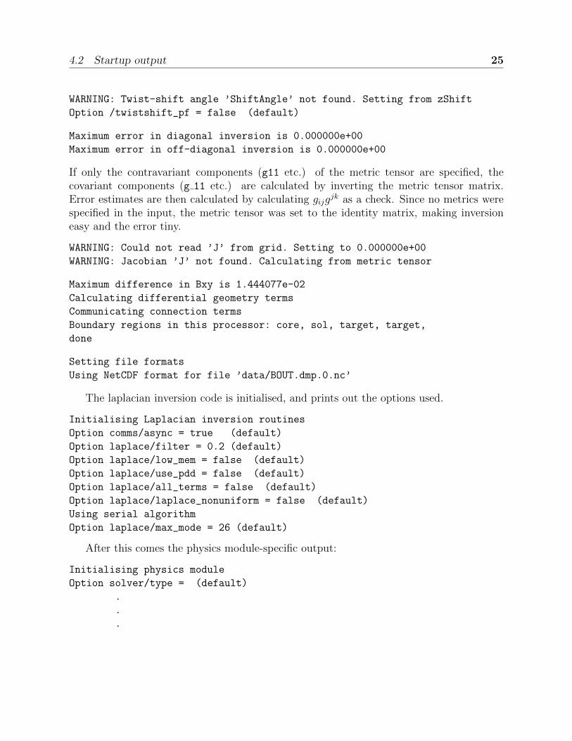
4.2 Startup output 25
WARNING: Twist-shift angle ’ShiftAngle’ not found. Setting from zShift
Option /twistshift_pf = false (default)
Maximum error in diagonal inversion is 0.000000e+00
Maximum error in off-diagonal inversion is 0.000000e+00
If only the contravariant components (g11 etc.) of the metric tensor are specified, thecovariant components (g 11 etc.) are calculated by inverting the metric tensor matrix.Error estimates are then calculated by calculating gijg
jk as a check. Since no metrics werespecified in the input, the metric tensor was set to the identity matrix, making inversioneasy and the error tiny.
WARNING: Could not read ’J’ from grid. Setting to 0.000000e+00
WARNING: Jacobian ’J’ not found. Calculating from metric tensor
Maximum difference in Bxy is 1.444077e-02
Calculating differential geometry terms
Communicating connection terms
Boundary regions in this processor: core, sol, target, target,
done
Setting file formats
Using NetCDF format for file ’data/BOUT.dmp.0.nc’
The laplacian inversion code is initialised, and prints out the options used.
Initialising Laplacian inversion routines
Option comms/async = true (default)
Option laplace/filter = 0.2 (default)
Option laplace/low_mem = false (default)
Option laplace/use_pdd = false (default)
Option laplace/all_terms = false (default)
Option laplace/laplace_nonuniform = false (default)
Using serial algorithm
Option laplace/max_mode = 26 (default)
After this comes the physics module-specific output:
Initialising physics module
Option solver/type = (default)
.
.
.
4.2 Startup output 26
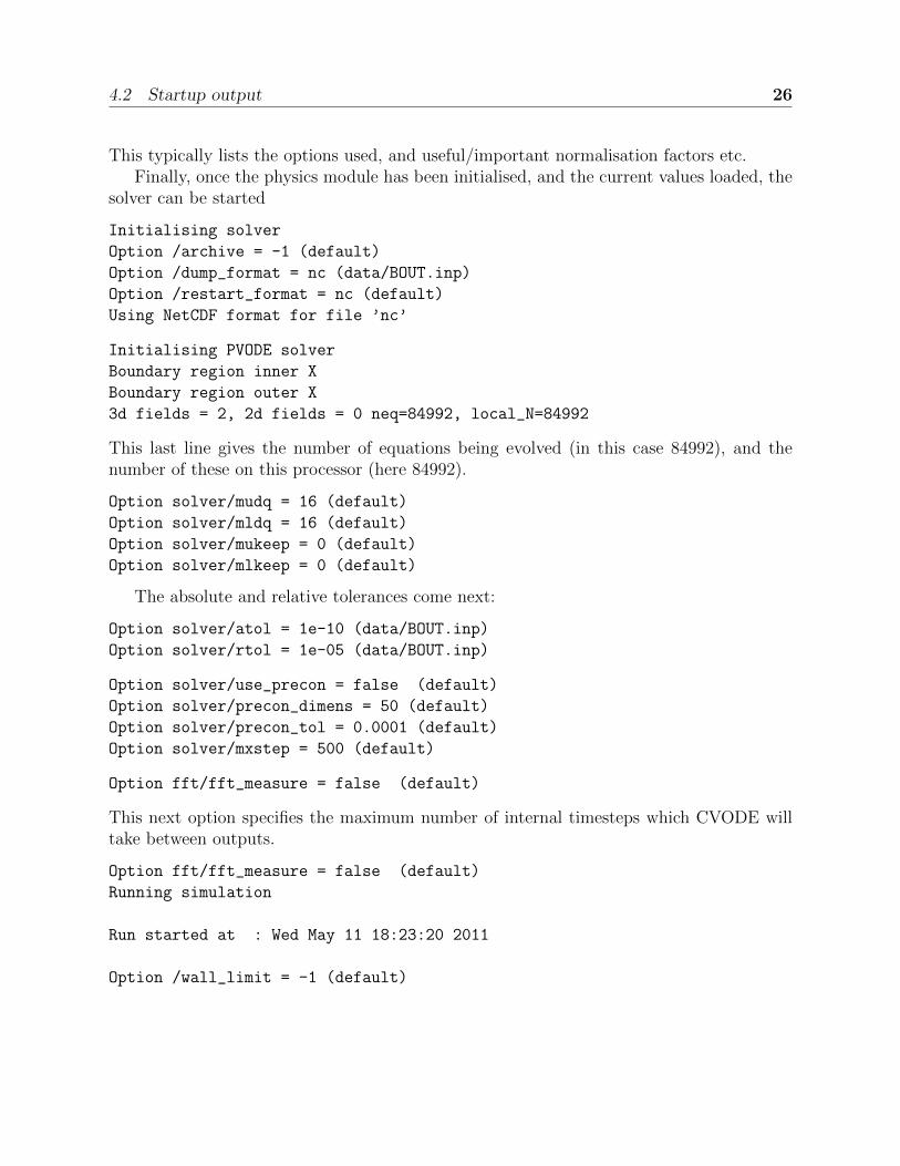
This typically lists the options used, and useful/important normalisation factors etc.Finally, once the physics module has been initialised, and the current values loaded, the
solver can be started
Initialising solver
Option /archive = -1 (default)
Option /dump_format = nc (data/BOUT.inp)
Option /restart_format = nc (default)
Using NetCDF format for file ’nc’
Initialising PVODE solver
Boundary region inner X
Boundary region outer X
3d fields = 2, 2d fields = 0 neq=84992, local_N=84992
This last line gives the number of equations being evolved (in this case 84992), and thenumber of these on this processor (here 84992).
Option solver/mudq = 16 (default)
Option solver/mldq = 16 (default)
Option solver/mukeep = 0 (default)
Option solver/mlkeep = 0 (default)
The absolute and relative tolerances come next:
Option solver/atol = 1e-10 (data/BOUT.inp)
Option solver/rtol = 1e-05 (data/BOUT.inp)
Option solver/use_precon = false (default)
Option solver/precon_dimens = 50 (default)
Option solver/precon_tol = 0.0001 (default)
Option solver/mxstep = 500 (default)
Option fft/fft_measure = false (default)
This next option specifies the maximum number of internal timesteps which CVODE willtake between outputs.
Option fft/fft_measure = false (default)
Running simulation
Run started at : Wed May 11 18:23:20 2011
Option /wall_limit = -1 (default)
4.3 Per-timestep output 27
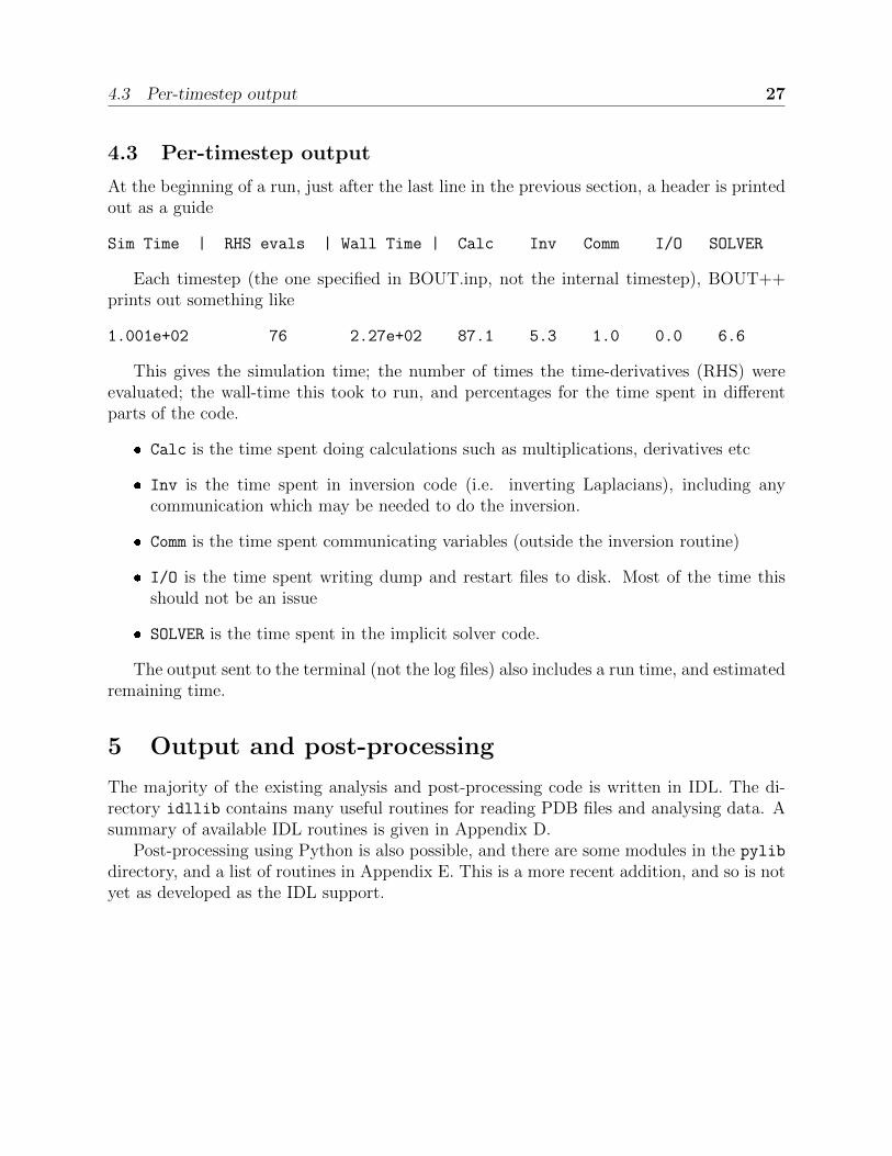
4.3 Per-timestep output
At the beginning of a run, just after the last line in the previous section, a header is printedout as a guide
Sim Time | RHS evals | Wall Time | Calc Inv Comm I/O SOLVER
Each timestep (the one specified in BOUT.inp, not the internal timestep), BOUT++prints out something like
1.001e+02 76 2.27e+02 87.1 5.3 1.0 0.0 6.6
This gives the simulation time; the number of times the time-derivatives (RHS) wereevaluated; the wall-time this took to run, and percentages for the time spent in differentparts of the code.
� Calc is the time spent doing calculations such as multiplications, derivatives etc
� Inv is the time spent in inversion code (i.e. inverting Laplacians), including anycommunication which may be needed to do the inversion.
� Comm is the time spent communicating variables (outside the inversion routine)
� I/O is the time spent writing dump and restart files to disk. Most of the time thisshould not be an issue
� SOLVER is the time spent in the implicit solver code.
The output sent to the terminal (not the log files) also includes a run time, and estimatedremaining time.
5 Output and post-processing
The majority of the existing analysis and post-processing code is written in IDL. The di-rectory idllib contains many useful routines for reading PDB files and analysing data. Asummary of available IDL routines is given in Appendix D.
Post-processing using Python is also possible, and there are some modules in the pylib
directory, and a list of routines in Appendix E. This is a more recent addition, and so is notyet as developed as the IDL support.
5.1 Note on reading PDB files 28
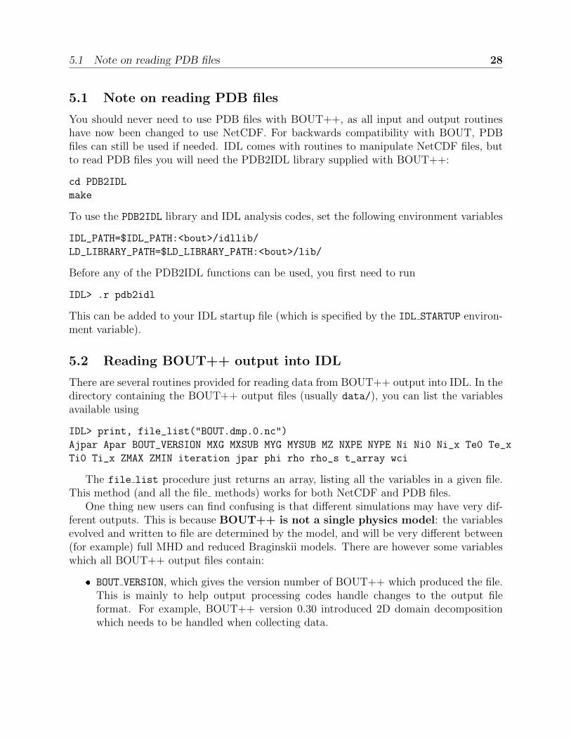
5.1 Note on reading PDB files
You should never need to use PDB files with BOUT++, as all input and output routineshave now been changed to use NetCDF. For backwards compatibility with BOUT, PDBfiles can still be used if needed. IDL comes with routines to manipulate NetCDF files, butto read PDB files you will need the PDB2IDL library supplied with BOUT++:
cd PDB2IDL
make
To use the PDB2IDL library and IDL analysis codes, set the following environment variables
IDL_PATH=$IDL_PATH:<bout>/idllib/
LD_LIBRARY_PATH=$LD_LIBRARY_PATH:<bout>/lib/
Before any of the PDB2IDL functions can be used, you first need to run
IDL> .r pdb2idl
This can be added to your IDL startup file (which is specified by the IDL STARTUP environ-ment variable).
5.2 Reading BOUT++ output into IDL
There are several routines provided for reading data from BOUT++ output into IDL. In thedirectory containing the BOUT++ output files (usually data/), you can list the variablesavailable using
IDL> print, file_list("BOUT.dmp.0.nc")
Ajpar Apar BOUT_VERSION MXG MXSUB MYG MYSUB MZ NXPE NYPE Ni Ni0 Ni_x Te0 Te_x
Ti0 Ti_x ZMAX ZMIN iteration jpar phi rho rho_s t_array wci
The file list procedure just returns an array, listing all the variables in a given file.This method (and all the file methods) works for both NetCDF and PDB files.
One thing new users can find confusing is that different simulations may have very dif-ferent outputs. This is because BOUT++ is not a single physics model: the variablesevolved and written to file are determined by the model, and will be very different between(for example) full MHD and reduced Braginskii models. There are however some variableswhich all BOUT++ output files contain:
� BOUT VERSION, which gives the version number of BOUT++ which produced the file.This is mainly to help output processing codes handle changes to the output fileformat. For example, BOUT++ version 0.30 introduced 2D domain decompositionwhich needs to be handled when collecting data.

5.2 Reading BOUT++ output into IDL 29
� MXG,MYG. These are the sizes of the X and Y guard cells
� MXSUB, the number of X grid points in each processor. This does not include the guardcells, so the total X size of each field will be MXSUB + 2*MXG.
� MYSUB, the number of Y grid points per processor (like MXSUB)
� MZ, the number of Z points
� NXPE, NYPE, the number of processors in the X and Y directions. NXPE * MXSUB +
2*MXG= NX, NYPE * MYSUB = NY
� ZMIN, ZMAX, the range of Z in fractions of 2π.
� iteration, the last timestep in the file
� t array, an array of times
Most of these - particularly those concerned with grid size and processor layout - are usedby post-processing routines such as collect, and are seldom needed directly. To read asingle variable from a file, there is the file read function:
IDL> wci = file_read("BOUT.dmp.0.nc", "wci")
IDL> print, wci
9.58000e+06
NOTE: The file read command (and NetCDF/PDB access generally) is case-sensitive: variable Wci is different to wci
To read in all the variables in a file into a structure, use the file import function:
IDL> d = file_import("BOUT.dmp.0.nc")
IDL> print, d.wci
9.58000e+06
This is often used to read in the entire grid file at once. Doing this for output data files cantake a long time and use a lot of memory.
Reading from individual files is fine for scalar quantities and time arrays, but readingarrays which are spread across processors (i.e. evolving variables) is tedious to do manually.Instead, there is the collect function to automate this:
IDL> ni = collect(var="ni")
Variable ’ni’ not found
-> Variables are case-sensitive: Using ’Ni’
Reading from .//BOUT.dmp.0.nc: [0-35][2-6] -> [0-35][0-4]
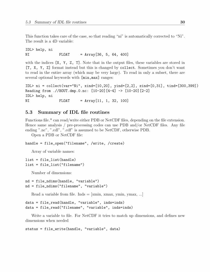
5.3 Summary of IDL file routines 30
This function takes care of the case, so that reading “ni” is automatically corrected to “Ni”.The result is a 4D variable:
IDL> help, ni
NI FLOAT = Array[36, 5, 64, 400]
with the indices [X, Y, Z, T]. Note that in the output files, these variables are stored in[T, X, Y, Z] format instead but this is changed by collect. Sometimes you don’t wantto read in the entire array (which may be very large). To read in only a subset, there areseveral optional keywords with [min,max] ranges:
IDL> ni = collect(var="Ni", xind=[10,20], yind=[2,2], zind=[0,31], tind=[300,399])
Reading from .//BOUT.dmp.0.nc: [10-20][4-4] -> [10-20][2-2]
IDL> help, ni
NI FLOAT = Array[11, 1, 32, 100]
5.3 Summary of IDL file routines
Functions file * can read/write either PDB or NetCDF files, depending on the file extension.Hence same analysis / pre-processing codes can use PDB and/or NetCDF files. Any fileending ”.nc”, ”.cdl”, ”.cdf” is assumed to be NetCDF, otherwise PDB.
Open a PDB or NetCDF file:
handle = file_open("filename", /write, /create)
Array of variable names:
list = file_list(handle)
list = file_list("filename")
Number of dimensions:
nd = file_ndims(handle, "variable")
nd = file_ndims("filename", "variable")
Read a variable from file. Inds = [xmin, xmax, ymin, ymax, ...]
data = file_read(handle, "variable", inds=inds)
data = file_read("filename", "variable", inds=inds)
Write a variable to file. For NetCDF it tries to match up dimensions, and defines newdimensions when needed
status = file_write(handle, "variable", data)

5.4 IDL analysis routines 31
Close a file after use
file_close, handle
To read in all the data in a file into a structure:
data = file_import("filename")
and to write a structure to file:
status = file_export("filename", data)
Converting file types can now be done using
d = file_import("somefile.pdb")
s = file_export("somefile.nc", d)
Note that this will mess up the case of the variable names, and names may be changedto become valid IDL variable names. To convert PDB files to NetCDF there is also a codepdb2cdf in BOUT/tools/archiving/pdb2cdf.
5.4 IDL analysis routines
Now that the BOUT++ results have been read into IDL, all the usual analysis and plottingroutines can be used. In addition, there are many useful routines included in the idllib
subdirectory. There is a README file which describes what each of these routines, but someof the most useful ones are listed here. All these examples assume there is a variable P
which has been read into IDL as a 4D [x,y,z,t] variable:
� fft deriv and fft integrate which differentiate and integrate periodic functions.
� get integer, get float, and get yesno request integers, floats and a yes/no answerfrom the user respectively.
� showdata animates 1 or 2-dimensional variables. Useful for quickly displaying resultsin different ways. This is useful for taking a quick look at the data, but can also pro-duce bitmap outputs for turning into a movie for presentation. To show an animatedsurface plot at a particular poloidal location (32 here):
IDL> showdata, p[*,32,*,*]
To turn this into a contour plot,
IDL> showdata, p[*,32,*,*], /cont

5.5 Python routines 32
To show a slice through this at a particular toroidal location (0 here):
IDL> showdata, p[*,32,0,*]
There are a few other options, and ways to show data using this code; see theREADME file, or comments in showdata.pro. Instead of plotting to screen, showdatacan produce a series of numbered bitmap images by using the bmp option
IDL> showdata, p[*,32,*,*], /cont, bmp="result_"
which will produce images called result 0000.bmp, result 0001.bmp and so on. Notethat the plotting should not be obscured or minimised, since this works by plottingto screen, then grabbing an image of the resulting plot.
� moment xyzt takes a 4D variable (such as those from collect), and calculates RMS,DC and AC components in the Z direction.
� safe colors A general routine for IDL which arranges the color table so that colorsare numbered 1 (black), 2 (red), 3 (green), 4 (blue). Useful for plotting, and used bymany other routines in this library.
There are many other useful routines in the idllib directory. See the idllib/README
file for a short description of each one.
5.5 Python routines
There are several modules available for reading NetCDF files, so to provide a consistent inter-face, file access is wrapped into a class DataFile. This provides a simple interface for readingand writing files from any of the following modules: netCDF4; Scientific.IO.NetCDF; andscipy.io.netcdf. To open a file using DataFile:
from boututils import DataFile
f = DataFile ("file.nc" ) # Open the f i l evar = f . read ("variable" ) # Read a v a r i a b l e from the f i l ef . close ( ) # Close the f i l e
To list the variables in a file e.g.
>>> f = DataFile ("test_io.grd.nc" )>>> print f . list ( )[ 'f3d' , 'f2d' , 'nx' , 'ny' , 'rvar' , 'ivar' ]
5.6 Matlab routines 33
and to list the names of the dimensions
>>> print d . dimensions ("f3d" )( 'x' , 'y' , 'z' )
or to get the sizes of the dimensions
>>> print d . size ("f3d" )[ 1 2 , 12 , 5 ]
To read in all variables in a file into a dictionary there is the file import function
1 from boututils import file_import
2
3 grid = file_import ("grid.nc" )
As for IDL, there is a collect routine which reads gathers together the data frommultiple processors
1 from boutdata import collect
2
3 Ni = collect ("Ni" ) # Collect the variable "Ni"
5.6 Matlab routines
There are Matlab routines for collecting data, showing animations, and performing somebasic analysis. See the tools/matlablib/ directory and README.txt file.
5.7 Mathematica routines
A package to read BOUT++ output data into Mathematica is in tools/mathematicalib.To read data into Mathematica, first add this directory to Mathematica’s path by putting
AppendTo[$Path,"<full_path_to_BOUT>/tools/mathematicalib"]
in your Mathematica startup file (usually \$HOME/.Mathematica/Kernel/init.m). To use thepackage, call
Import["BoutCollect.m"]
from inside Mathematica. Then you can use e.g.
f=BoutCollect[variable,path->"data"]
or
f=BoutCollect[variable,path->"data"]
’bc’ is a shorthand for ’BoutCollect’. All options supported by the Python collect()←↩function are included, though Info does nothing yet.

5.8 Octave routines 34
5.8 Octave routines
There is minimal support for reading data into Octave, which has been tested on Octave3.2. It requires the octcdf library to access NetCDF files.
f = bcollect ( ) # o pt i o na l path argument i s ” . ” by d e f a u l t
f = bsetxrange (f , 1 , 10) # Set ranges# Same f o r y , z , and t (NOTE: index ing from 1 ! )
u = bread (f , "U" ) # F i n a l l y read the v a r i a b l e
6 BOUT++ options
The inputs to BOUT++ are a binary grid file in NetCDF or PDB format, and a text filewith options. Generating input grids for tokamaks is described in section 7. The grid filedescribes the size and topology of the X-Y domain, metric tensor components and usuallysome initial profiles. The option file specifies the size of the domain in the symmetricdirection (Z), and controls how the equations are evolved e.g. differencing schemes to use,and boundary conditions. In most situations, the grid file will be used in many differentsimulations, but the options may be changed frequently.
The text input file BOUT.inp is always in a subdirectory called data for all examples. Thefiles include comments (starting with either ’;’ or ’#’) and should be fairly self-explanatory.The format is the same as a windows INI file, consisting of name = value pairs. Commentsare started with a hash (#) or semi-colon, which comments out the rest of the line. valuescan be:
� Integers
� Real values
� Booleans
� Strings
Options are also divided into sections, which start with the section name in square brackets.
[ section1 ]
something = 132 # an i n t e g e ranother = 5.131 # a r e a l va lueyetanother = true # a booleanfinally = "some text" # a s t r i n g

6.1 Command line options 35
NOTE: Options are NOT case-sensitive: TwistShift and twistshift are thesame variable
Subsections can also be used, separated by colons ’:’, e.g.
[ section : subsection ]
Have a look through the examples to see how the options are used.
6.1 Command line options
All options can be set on the command line, and will override those set in BOUT.inp. Themost commonly used are “restart” and “append”, described in section 4. If values are notgiven for command-line arguments, then the value is set to true, so putting restart isequivalent to restart=true.
Values can be specified on the command line for other settings, such as the fraction ofa torus to simulate (ZPERIOD):
./command zperiod=10
Remember no spaces around the ’=’ sign. Like the BOUT.inp file, setting names are notcase sensitive.
Sections are separated by colons ’:’, so to set the solver type (section 6.3) you can eitherput this in BOUT.inp:
[solver]
type = rk4
or put solver:type=rk4 on the command line. This capability is used in many test suitecases to change the parameters for each run.
6.2 General options
At the top of the BOUT.inp file (before any section headers), options which affect the corecode are listed. These are common to all physics models, and the most useful of them are:
NOUT = 100 # number o f time−po in t s outputTIMESTEP = 1.0 # time between outputs
which set the number of outputs, and the time step between them. Note that this hasnothing to do with the internal timestep used to advance the equations, which is adjustedautomatically. What time-step to use depends on many factors, but for high-β reducedMHD ELM simulations reasonable choices are 1.0 for the first part of a run (to handleinitial transients), then around 10.0 for the linear phase. Once non-linear effects becomeimportant, you will have to reduce the timestep to around 0.1.

6.2 General options 36
Most large clusters or supercomputers have a limit on how long a job can run for called“wall time”, because it’s the time taken according to a clock on the wall, as opposed to theCPU time actually used. If this is the case, you can use the option
wall_limit = 10 # wal l c l o ck l i m i t ( in hours )
BOUT++ will then try to quit cleanly before this time runs out. Setting a negative value(default is -1) means no limit.
Often it’s useful to be able to restart a simulation from a chosen point, either to reproducea previous run, or to modify the settings and re-run. A restart file is output every timestep,but this is overwritten each time, and so the simulation can only be continued from the endof the last simulation. Whilst it is possible to create a restart file from the output dataafterwards, it’s much easier if you have the restart files. Using the option
archive = 20
saves a copy of the restart files every 20 timesteps, which can then be used as a startingpoint.
The X and Y size of the computational grid is set by the grid file, but the number ofpoints in the Z (axisymmetric) direction is specified in the options file:
MZ = 33
This must be MZ = 2n + 1, and can be 2, 3, 5, 9, . . .. The power of 2 is so that FFTs can beused in this direction; the +1 is for historical reasons (inherited from BOUT) and is goingto be removed at some point.
Since the Z dimension is periodic, the domain size is specified as multiples or fractionsof 2π. To specify a fraction of 2π, use
ZPERIOD = 10
This specifies a Z range from 0 to 2π/ZPERIOD, and is useful for simulation of tokamaks tomake sure that the domain is an integer fraction of a torus. If instead you want to specifythe Z range directly (for example if Z is not an angle), there are the options
ZMIN = 0.0ZMAX = 0.1
which specify the range in multiples of 2π.
NOTE: For users of BOUT, the definition of ZMIN and ZMAX has been changed.These are now fractions of 2π radians i.e. dz = 2π(ZMAX - ZMIN)/(MZ-1)
In BOUT++, grids can be split between processors in both X and Y directions. Bydefault only Y decomposition is used, and to use X decomposition you must specify thenumber of processors in the X direction:
NXPE = 1 # Set number o f X p r o c e s s o r s

6.3 Time integration solver 37
The grid file to use is specified relative to the root directory where the simulation is run(i.e. running “ls ./data/BOUT.inp” gives the options file)
grid = "data/cbm18_8_y064_x260.pdb"
6.3 Time integration solver
BOUT++ can be compiled with several different time-integration solvers (see section ??),and at minimum should have Runge-Kutta (RK4) and PVODE (BDF/Adams) solvers avail-able.
The solver library used is set using the solver:type option, so either in BOUT.inp:
[ solver ]type = rk4 # Set the s o l v e r to use
or on the command line by adding solver:type=pvode for example:
mpirun −np 4 ./2 fluid solver : type=rk4
NB: Make sure there are no spaces around the “=” sign: solver:type =pvode won’t work(probably). Table 9 gives a list of time integration solvers, along with any compile-timeoptions needed to make the solver available.
Table 1: Available time integration solversName Description Compile optionseuler Euler explicit method Always availablerk4 Runge-Kutta 4th-order explicit method Always available
karniadakis Karniadakis explicit method Always availablepvode 1998 PVODE with BDF method Always availablecvode SUNDIALS CVODE. BDF and Adams methods –with-cvode
ida SUNDIALS IDA. DAE solver –with-idapetsc PETSc TS methods –with-petsc
Each solver can have its own settings which work in slightly different ways, but somecommon settings and which solvers they are used in are given in table 2. The most commonlychanged options are the absolute and relative solver tolerances, ATOL and RTOL which shouldbe varied to check convergence.
6.4 Input and Output
The output (dump) files with time-history are controlled by settings in a section called“output”. Restart files contain a single time-slice, and are controlled by a section called“restart”. The options available are listed in table 3.
6.4 Input and Output 38
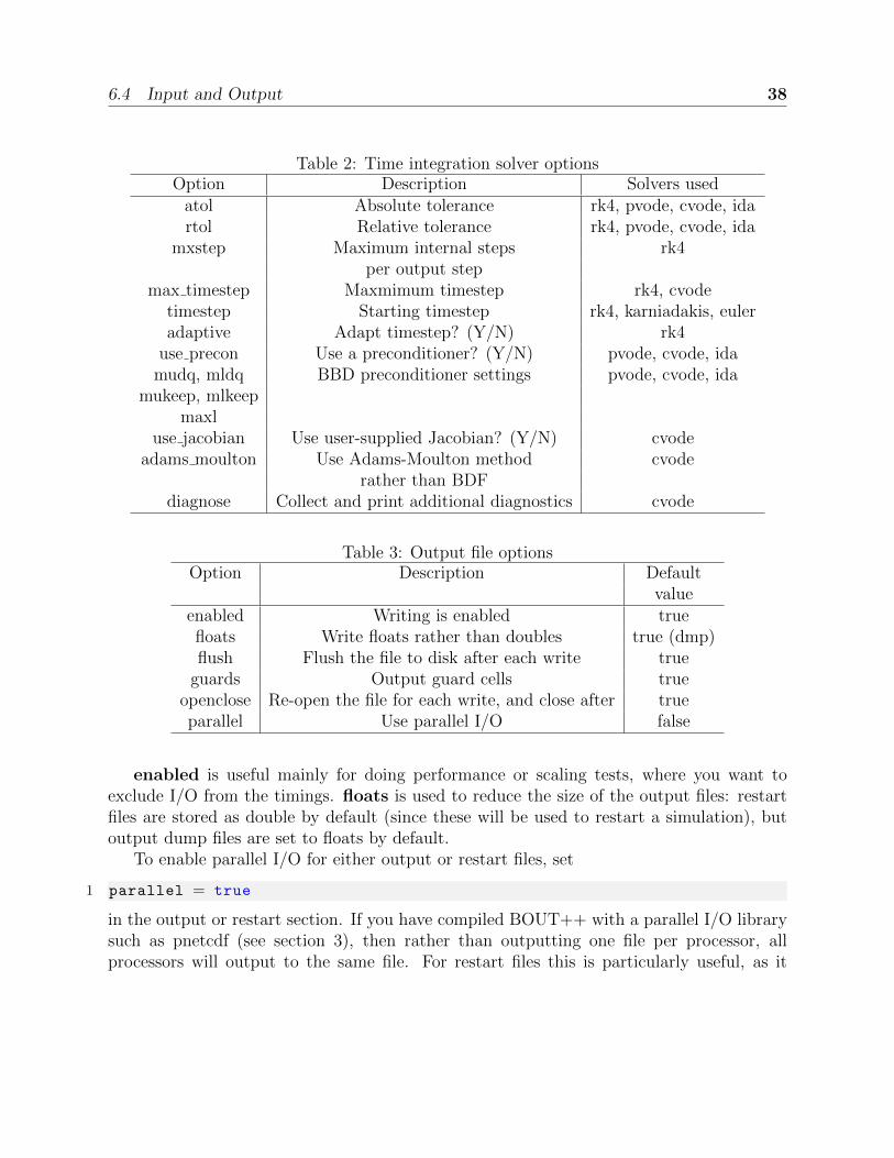
Table 2: Time integration solver optionsOption Description Solvers used
atol Absolute tolerance rk4, pvode, cvode, idartol Relative tolerance rk4, pvode, cvode, ida
mxstep Maximum internal steps rk4per output step
max timestep Maxmimum timestep rk4, cvodetimestep Starting timestep rk4, karniadakis, euleradaptive Adapt timestep? (Y/N) rk4
use precon Use a preconditioner? (Y/N) pvode, cvode, idamudq, mldq BBD preconditioner settings pvode, cvode, ida
mukeep, mlkeepmaxl
use jacobian Use user-supplied Jacobian? (Y/N) cvodeadams moulton Use Adams-Moulton method cvode
rather than BDFdiagnose Collect and print additional diagnostics cvode
Table 3: Output file optionsOption Description Default
valueenabled Writing is enabled truefloats Write floats rather than doubles true (dmp)flush Flush the file to disk after each write true
guards Output guard cells trueopenclose Re-open the file for each write, and close after trueparallel Use parallel I/O false
enabled is useful mainly for doing performance or scaling tests, where you want toexclude I/O from the timings. floats is used to reduce the size of the output files: restartfiles are stored as double by default (since these will be used to restart a simulation), butoutput dump files are set to floats by default.
To enable parallel I/O for either output or restart files, set
1 parallel = true
in the output or restart section. If you have compiled BOUT++ with a parallel I/O librarysuch as pnetcdf (see section 3), then rather than outputting one file per processor, allprocessors will output to the same file. For restart files this is particularly useful, as it

6.5 Laplacian inversion 39
means that you can restart a job with a different number of processors. Note that thisfeature is still experimental, and incomplete: output dump files are not yet supported bythe collect routines.
6.5 Laplacian inversion
A common problem in plasma models is to solve an equation of the form
d∇2⊥x+
1
c∇⊥c · ∇⊥x+ ax = b
where x and b are 3D variables, whilst a, c and d are 2D variables. BOUT++ includesseveral routines for solving this equation; see the developer’s manual for details.
Table 4: Global Laplacian optionsOption Description Defaultlow mem Reduces memory usage false
use pdd Use the PDD algorithm false
all terms Include all terms false
laplace nonuniform Non-uniform mesh corrections false
filter Fraction of modes to filter 0.2max mode Maximum Z mode filter
6.6 Communications
The communication system has a section [comms], with a true/false option async. Thisdetermines whether asyncronous MPI sends are used; which method is faster varies (thoughnot by much) with machine and problem.
6.7 Differencing methods
Differencing methods are specified in three section ([ddx], [ddy] and [ddz]), one for eachdimension.
� first, the method used for first derivatives
� second, method for second derivatives
� upwind, method for upwinding terms
� flux, for conservation law terms
6.8 Model-specific options 40
The methods which can be specified are U1, U4, C2, C4, W2, W3, FFT Apart from FFT,the first letter gives the type of method (U = upwind, C = central, W = WENO), and thenumber gives the order.
6.8 Model-specific options
The options which affect a specific physics model vary, since they are defined in the physicsmodule itself (see section 8.3). They should have a separate section, for example the high-βreduced MHD code uses options in a section called [highbeta].
There are three places to look for these options: the BOUT.inp file; the physics modelC++ code, and the output logs. The physics module author should ideally have an exampleinput file, with commented options explaining what they do; alternately they may have putcomments in the C++ code for the module. Another way is to look at the output logs: whenBOUT++ is run, (nearly) all options used are printed out with their default values. Thiswon’t provide much explanation of what they do, but may be useful anyway. See section 5for more details.
6.9 Variable initialisation
Each variable being evolved has its own section, with the same name as the output data.For example, the high-β model has variables “P”, “jpar”, and “U”, and so has sections [P],[jpar], [U] (not case sensitive).
There are two ways to specify the initial conditions for a variable: the original method(similar to that used by BOUT-06) which covers the most commonly needed functions. Ifmore flexibility is needed then a more general analytical expression can be given.
6.9.1 Original method
The shape of the initial value is specified for each dimension separately using the optionsxs opt, ys opt, and zs opt. These are set to an integer:
0. Constant (this is the default)
1. Gaussian, with a peak location given by xs s0, ys s0, zs s0 as a fraction of thedomain (i.e. 0 → 1. The width is given by *s wd, also as a fraction of the domainsize.
2. Sinusoidal, with the number of periods given by *s mode.
3. Mix of mode numbers, with psuedo-random phases.

6.9 Variable initialisation 41
The magnitude of the initial value is given by the variable scale.Defaults for all variables can be set in a section called [All], so for example the options
below:
[ All ]scale = 0.0 # By d e f a u l t s e t v a r i a b l e s to zero
xs_opt = 1 # Gaussian in Xys_opt = 1 # Gaussian in Yzs_opt = 2 # S i n u s o i d a l in Z ( axisymmetric d i r e c t i o n )
xs_s0 = 0.5 # Peak in the middle o f the X d i r e c t i o nxs_wd = 0.1 # Width i s 10% of the domain
ys_s0 = 0.5 # Peak in the middle o f the Y d i r e c t i o nys_wd = 0.3 # Width i s 30% of the Y domain
zs_mode = 3 # 3 per i od s in the Z d i r e c t i o n
[ U ]scale = 1.0e−5 # Amplitude f o r the U var i ab l e , o v e r r i d e s d e f a u l t
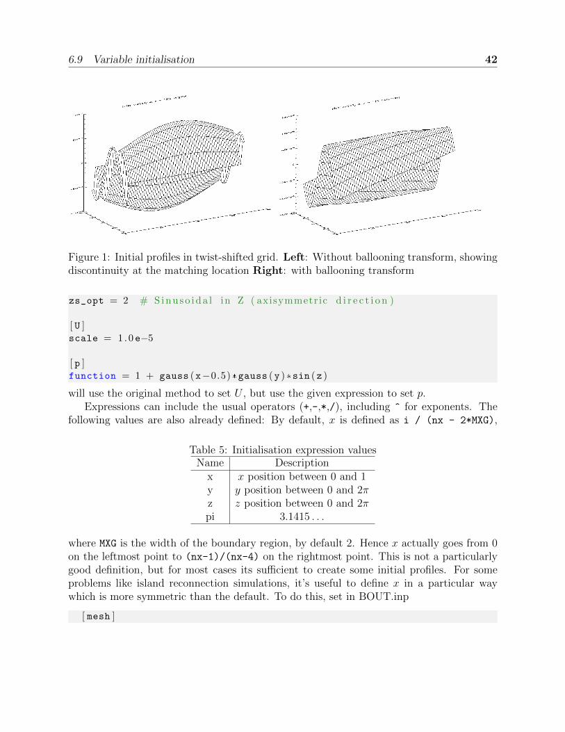
For field-aligned tokamak simulations, the Y direction is along the field and in the corethis will have a discontinuity at the twist-shift location where field-lines are matched ontoeach other. To handle this, a truncated Ballooning transformation can be used to constructa smooth initial perturbation:
U balloon0 =
N∑i=−N
F (x)G (y + 2πi)H (z + q2πi)
NOTE: The initial profiles code currently doesn’t work very well for grids withbranch-cuts (e.g. divertor tokamak), and will often have jumps which then maketimesteps smaller
6.9.2 Expressions
If a more general function is needed, a variable can be initialised using the function optionfor each variable. This overrides the original method for that variable. e.g.
[ all ]
xs_opt = 1 # Gaussian in Xys_opt = 1 # Gaussian in Y
6.9 Variable initialisation 42
Figure 1: Initial profiles in twist-shifted grid. Left: Without ballooning transform, showingdiscontinuity at the matching location Right: with ballooning transform
zs_opt = 2 # S i n u s o i d a l in Z ( axisymmetric d i r e c t i o n )
[ U ]scale = 1.0e−5
[ p ]function = 1 + gauss (x−0.5)*gauss (y ) *sin (z )
will use the original method to set U , but use the given expression to set p.Expressions can include the usual operators (+,-,*,/), including ^ for exponents. The
following values are also already defined: By default, x is defined as i / (nx - 2*MXG),
Table 5: Initialisation expression valuesName Description
x x position between 0 and 1y y position between 0 and 2πz z position between 0 and 2πpi 3.1415 . . .
where MXG is the width of the boundary region, by default 2. Hence x actually goes from 0on the leftmost point to (nx-1)/(nx-4) on the rightmost point. This is not a particularlygood definition, but for most cases its sufficient to create some initial profiles. For someproblems like island reconnection simulations, it’s useful to define x in a particular waywhich is more symmetric than the default. To do this, set in BOUT.inp
[ mesh ]
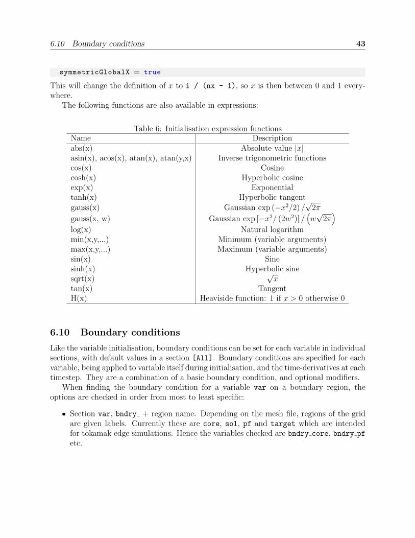
6.10 Boundary conditions 43
symmetricGlobalX = true
This will change the definition of x to i / (nx - 1), so x is then between 0 and 1 every-where.
The following functions are also available in expressions:
Table 6: Initialisation expression functionsName Descriptionabs(x) Absolute value |x|asin(x), acos(x), atan(x), atan(y,x) Inverse trigonometric functionscos(x) Cosinecosh(x) Hyperbolic cosineexp(x) Exponentialtanh(x) Hyperbolic tangent
gauss(x) Gaussian exp (−x2/2) /√
2π
gauss(x, w) Gaussian exp [−x2/ (2w2)] /(w√
2π)
log(x) Natural logarithmmin(x,y,...) Minimum (variable arguments)max(x,y,...) Maximum (variable arguments)sin(x) Sinesinh(x) Hyperbolic sinesqrt(x)
√x
tan(x) TangentH(x) Heaviside function: 1 if x > 0 otherwise 0
6.10 Boundary conditions
Like the variable initialisation, boundary conditions can be set for each variable in individualsections, with default values in a section [All]. Boundary conditions are specified for eachvariable, being applied to variable itself during initialisation, and the time-derivatives at eachtimestep. They are a combination of a basic boundary condition, and optional modifiers.
When finding the boundary condition for a variable var on a boundary region, theoptions are checked in order from most to least specific:
� Section var, bndry + region name. Depending on the mesh file, regions of the gridare given labels. Currently these are core, sol, pf and target which are intendedfor tokamak edge simulations. Hence the variables checked are bndry core, bndry pf
etc.

6.10 Boundary conditions 44
� Section var, bndry + boundary side. These names are xin, xout, yup and ydown.
� Section var, variable bndry all
� The same settings again except in section All.
The default setting for everything is therefore bndry all in the All section.Boundary conditions are given names, with optional arguments in brackets. Currently
implemented boundary conditions are:
� dirichlet - Set to zero
� dirichlet(<number>) - Set to some number e.g. dirichlet(1) sets the boundaryto 1.0
� neumann - Zero gradient
� robin - A combination of zero-gradient and zero-value af + b∂f∂x
= g where the syntaxis robin(a, b, g).
� constgradient - Constant gradient across boundary
� zerolaplace - Laplacian = 0, decaying solution (X boundaries only)
� zerolaplace2 - Laplacian = 0, using coefficients from the Laplacian inversion andDelp2 operator.
� constlaplace - Laplacian = const, decaying solution (X boundaries only)
The zero- or constant-Laplacian boundary conditions works as follows:
∇2⊥f = 0
' gxx∂2f
∂x2+ gzz
∂2f
∂z2
which when Fourier transformed in z becomes:
gxx∂2f̂
∂x2− gzzk2z f̂ = 0
which has the solutionf̂ = Aexkz
√gzz/gxx +Be−xkz
√gzz/gxx
Assuming that the solution should decay away from the domain, on the inner x boundaryB = 0, and on the outer boundary A = 0.
Boundary modifiers change the behavior of boundary conditions, and more than onemodifier can be used. Currently the following are available:

6.10 Boundary conditions 45
� relax - Relaxing boundaries. Evolve the variable towards the given boundary condi-tion at a given rate
� shifted - Apply boundary conditions in orthogonal X-Z coordinates, rather thanfield-aligned
� width - Modifies the width of the region over which the boundary condition is applied
These are described in the following subsections.
6.10.1 Relaxing boundaries
All boundaries can be modified to be “relaxing” which are a combination of zero-gradienttime-derivative, and whatever boundary condition they are applied to. The idea is that thisprevents sharp discontinuities at boundaries during transients, whilst maintaining the de-sired boundary condition on longer timescales. In some cases this can improve the numericalstability and timestep.
For example, relax(dirichlet) will make a field f at point i in the boundary follow apoint i− 1 in the domain:
∂f
∂t
∣∣∣∣∣i
=∂f
∂t
∣∣∣∣∣i−1− fi/τ
where τ is a timescale for the boundary (currently set to 0.1, but will be a global option).When the time-derivatives are slow close to the boundary, the boundary relaxes to thedesired condition (Dirichlet in this case), but when the time-derivatives are large then theboundary approaches Neumann to reduce discontinuities.
By default, the relaxation rate is set to 10 (i.e. a timescale of τ = 0.1). To change this,give the rate as the second argument e.g. relax(dirichlet, 2) would relax to a Dirichletboundary condition at a rate of 2.
6.10.2 Shifted boundaries
By default boundary conditions are applied in field-aligned coordinates, where y is alongfield-lines but x has a discontinuity at the twist-shift location. If radial derivatives are beingdone in shifted coordinates where x and z are orthogonal, then boundary conditions shouldalso be applied in shifted coordinates. To do this, the shifted boundary modifier appliesa z shift, applies the boundary condition, then shifts back. For example:
bndry_core = shifted ( neumann )
would ensure that radial derivatives were zero in shifted coordinates on the core boundary.

6.10 Boundary conditions 46
6.10.3 Changing the width of boundaries
To change the width of a boundary region, the width modifier changes the width of aboundary region before applying the boundary condition, then changes the width backafterwards. To use, specify the boundary condition and the width, for example
bndry_core = width ( neumann , 4 )
would apply a Neumann boundary condition on the innermost 4 cells in the core, ratherthan the usual 2. When combining with other boundary modifiers, this should be appliedfirst e.g.
bndry_sol = width ( relax ( dirichlet ) , 3)
would relax the last 3 cells towards zero, whereas
bndry_sol = relax ( width ( dirichlet , 3) )
would only apply to the usual 2, since relax didn’t use the updated width.Limitations:
1. Because it modifies then restores a globally-used BoundaryRegion, this code is notthread safe.
2. Boundary conditions can’t be applied across processors, and no checks are done thatthe width asked for fits within a single processor.
6.10.4 Examples
This example is taken from the UEDGE benchmark test (in examples/uedge-benchmark):
[ All ]bndry_all = neumann # Defau l t f o r a l l v a r i a b l e s , boundar ies
[ Ni ]bndry_target = neumann
bndry_core = relax ( dirichlet ( 1 . ) ) # 1 e13 cmˆ−3 on core boundarybndry_all = relax ( dirichlet ( 0 . 1 ) ) # 1 e12 cmˆ−3 on other boundar ies
[ Vi ]bndry_ydown = relax ( dirichlet (−1.41648) ) # −3.095 e4/ Vi xbndry_yup = relax ( dirichlet ( 1 .41648) )
The variable Ni (density) is set to a Neumann boundary condition on the targets (yupand ydown), relaxes towards 1 on the core boundary, and relaxes to 0.1 on all other bound-aries. Note that the bndry target = neumann needs to be in the Ni section: If we justhad
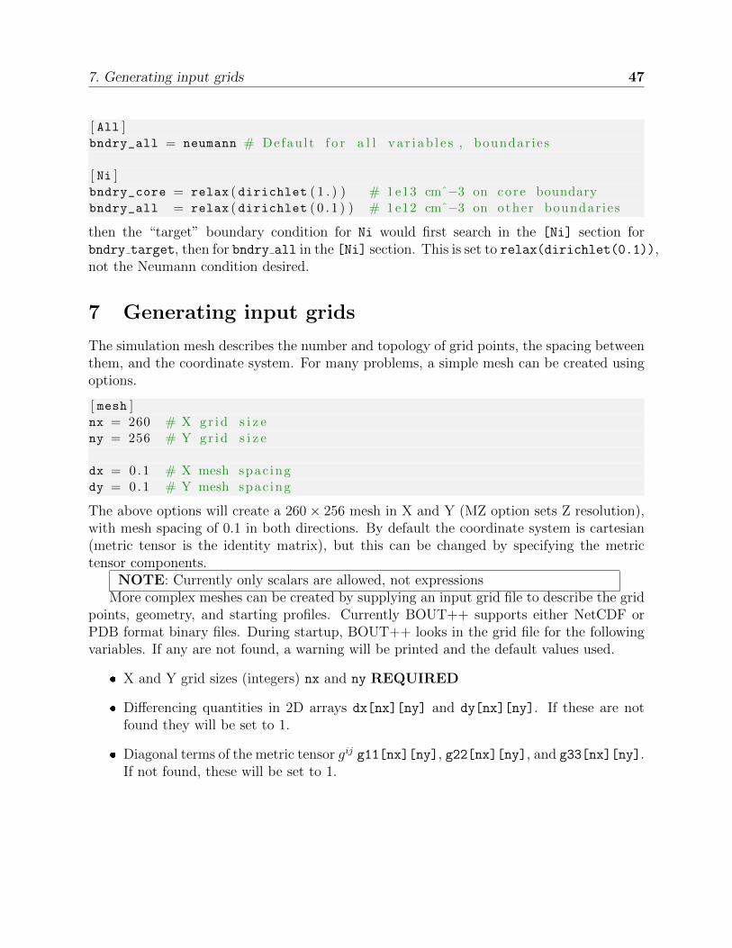
7. Generating input grids 47
[ All ]bndry_all = neumann # Defau l t f o r a l l v a r i a b l e s , boundar ies
[ Ni ]bndry_core = relax ( dirichlet ( 1 . ) ) # 1 e13 cmˆ−3 on core boundarybndry_all = relax ( dirichlet ( 0 . 1 ) ) # 1 e12 cmˆ−3 on other boundar ies
then the “target” boundary condition for Ni would first search in the [Ni] section forbndry target, then for bndry all in the [Ni] section. This is set to relax(dirichlet(0.1)),not the Neumann condition desired.
7 Generating input grids
The simulation mesh describes the number and topology of grid points, the spacing betweenthem, and the coordinate system. For many problems, a simple mesh can be created usingoptions.
[ mesh ]nx = 260 # X gr id s i z eny = 256 # Y gr id s i z e
dx = 0.1 # X mesh spac ingdy = 0.1 # Y mesh spac ing
The above options will create a 260× 256 mesh in X and Y (MZ option sets Z resolution),with mesh spacing of 0.1 in both directions. By default the coordinate system is cartesian(metric tensor is the identity matrix), but this can be changed by specifying the metrictensor components.
NOTE: Currently only scalars are allowed, not expressionsMore complex meshes can be created by supplying an input grid file to describe the grid
points, geometry, and starting profiles. Currently BOUT++ supports either NetCDF orPDB format binary files. During startup, BOUT++ looks in the grid file for the followingvariables. If any are not found, a warning will be printed and the default values used.
� X and Y grid sizes (integers) nx and ny REQUIRED
� Differencing quantities in 2D arrays dx[nx][ny] and dy[nx][ny]. If these are notfound they will be set to 1.
� Diagonal terms of the metric tensor gij g11[nx][ny], g22[nx][ny], and g33[nx][ny].If not found, these will be set to 1.

7.1 From EFIT files 48
� Off-diagonal metric tensor gij elements g12[nx][ny], g13[nx][ny], and g23[nx][ny].If not found, these will be set to 0.
� Z shift for sheared grids zshift[nx][ny]. This is intended for dpsi derivatives insheared coordinates. If not found, set to zero.
The remaining quantities determine the topology of the grid. These are based on tokamaksingle/double-null configurations, but can be adapted to many other situations.
� Separatrix locations ixseps1, and ixseps2 If neither is given, both are set to nx (i.e.all points in closed “core” region). If only ixseps1 is found, ixseps2 is set to nx, andif only ixseps2 is found, ixseps1 is set to -1.
� Branch-cut locations jyseps1 1, jyseps1 2, jyseps2 1, and jyseps2 2
� Twist-shift matching condition twistshift[nx]. This is applied in the “core” regionbetween indices jyseps2 2, and jyseps1 1 + 1, if enabled in the options file. If notgiven, this is set to zero.
NOTE: All input quantities should be normalised - no normalisation is performedby the BOUT++ code. Normalisation can be performed in the initialisation code,provided a call to geometry() is made after any changes to the metrics.For users of BOUT, the radial derivative is dx = dpsi / (bmag/1e4)
The only quantities which are required are the sizes of the grid. If these are the onlyquantities specified, then the coordinates revert to cartesian.
This section describes how to generate inputs for tokamak equilibria. If you’re notinterested in tokamaks then you can skip to the next section.
The directory tokamak grids contains code to generate input grid files for tokamaks.These can be used by the 2fluid and highbeta reduced modules, and are (mostly) com-patible with inputs to the BOUT-06 code.
Figure 2 shows the routines and file formats used in taking output from different codesand converting into input to BOUT++.
7.1 From EFIT files
An IDL code called “Hypnotoad” has been developed to create BOUT++ input files from R-Z equilibria. This can read EFIT ’g’ files, find flux surfaces, and calculate metric coefficients.The code is in tools/tokamak grids/gridgen, and has its own manual under the docsubdirectory.

7.1 From EFIT files 49
UEDGE
shifted circle
uedgegrd.pdb
uedge.pdb
UEDGE OUTPUT
uedge2bout.pro pdb2bout.pro
bout output.pro
BOUT++ GRID
PDB G-S FILE
elite2pdb gato2pdb
ELITE EQIN DSKGATO
TOQ, CORSICASCENE, ...
Grad-shafranov
EXTERNAL CODES SUPPLYING EQUILIBRIA
Figure 2: Generation of BOUT++ grid files. In red are the file formats, and in black theconversion routines. Blue are external codes.

7.2 From ELITE and GATO files 50
7.2 From ELITE and GATO files
Currently conversions exist for ELITE .eqin and GATO dskgato equilibrium files. Conver-sion of these into BOUT++ input grids is in two stages: In the first, both these input filesare converted into a common NetCDF or PDB format which describes the Grad-Shafranovequilibrium. These intermediate files are then converted to BOUT++ grids using an inter-active IDL script.
7.3 Generating equilibria
The directory tokamak grids/shifted circle contains IDL code to generate shifted circle(large aspect ratio) Grad-Shafranov equilibria.
7.4 Running pdb2bout
There are many options which are set interactively, so here’s a run-through of the code (onlyshowing most important outputs):
IDL> pdb2bout, "cbm18_dens6.dskgato.pdb", output="test.pdb"
***Maximum mu0p is 23071.7
Is this pressure (not mu0*pressure)?
This is needed because although many grid formats claim to store µ0P , they actually storeP . Since the given maximum value is very large, it must be in Pascals, so answer yes (y).
The grid will then be displayed along with the safety factor and pressure profiles againstnormalised ψ. In all three plots, a red line marks the location of the plasma edge. You mustthen choose the radial domain in normalised ψ:
Inner Psi boundary:0.6
Outer Psi boundary:1.2
Number of radial grid points: 69
Of which inside the plasma: 49
Is this range ok?
The plots will now also show two green lines for the inner and outer boundaries. Enter no(n) to specify a different range.
The code then checks to see if any plasma density of temperatures have been set in theinput file:
====== SETTING PLASMA PROFILES =======
Some plasma parameters given in input file
Use given parameters?

7.4 Running pdb2bout 51
Saying yes will just use the given values, but saying no will give you some more options:
Generating plasma profiles:
1. Flat temperature profile
2. Flat density profile
3. Te proportional to density
Profile option:
The procedure is the same for each of these, so taking option 2 (flat density):
Setting flat density profile
Density [10^20 m^-3]:1.0
Anything can be entered here, depending on what you want to simulate. The code willensure that whatever you enter, the equilibrium pressure is maintained. In this case thetemperature is calculated from pressure and the specified density.
Maximum temperature (eV): 720.090
Is this ok?
NOTE: This is the maximum temperature anywhere on the input grid (i.e. in this case atψ = 0), not just inside the chosen domain. Entering no will go back and you can specify adifferent density.
Earlier the radial resolution was printed, in this case 69 grid points. You can now changethis if you need to:
Increase radial resolution?
Although it says increase, you can also decrease the resolution. Entering yes will allow youto enter a different number of radial grid points. It’s recommended to use 2n + 4 grid pointsbecause this makes it easier to decompose the grid (4 cells for boundary, remainder equallydivided between processors).
At this point, an orthogonal grid is generated:
======== GENERATING ORTHOGONAL COORDINATES FOR BOUT =========
Number of poloidal grid points: 64
Enter x index of equal hthe [0, 68] :35
Using 2n points is highly recommended, but only because the points must be equally dividedbetween processors. The x index of equal hthe shouldn’t matter very much except for highlyshaped plasmas. Recommend that you set it somewhere around the peak pressure gradient,or middle of the grid.
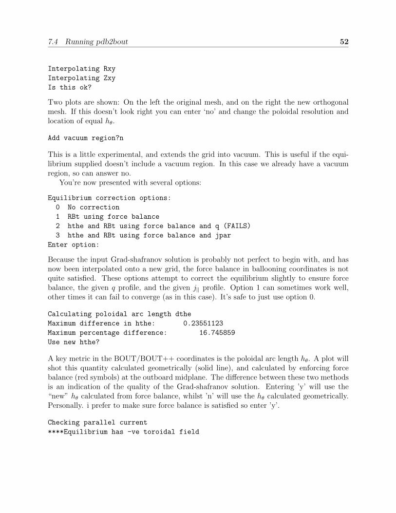
7.4 Running pdb2bout 52
Interpolating Rxy
Interpolating Zxy
Is this ok?
Two plots are shown: On the left the original mesh, and on the right the new orthogonalmesh. If this doesn’t look right you can enter ‘no’ and change the poloidal resolution andlocation of equal hθ.
Add vacuum region?n
This is a little experimental, and extends the grid into vacuum. This is useful if the equi-librium supplied doesn’t include a vacuum region. In this case we already have a vacuumregion, so can answer no.
You’re now presented with several options:
Equilibrium correction options:
0 No correction
1 RBt using force balance
2 hthe and RBt using force balance and q (FAILS)
3 hthe and RBt using force balance and jpar
Enter option:
Because the input Grad-shafranov solution is probably not perfect to begin with, and hasnow been interpolated onto a new grid, the force balance in ballooning coordinates is notquite satisfied. These options attempt to correct the equilibrium slightly to ensure forcebalance, the given q profile, and the given j|| profile. Option 1 can sometimes work well,other times it can fail to converge (as in this case). It’s safe to just use option 0.
Calculating poloidal arc length dthe
Maximum difference in hthe: 0.23551123
Maximum percentage difference: 16.745859
Use new hthe?
A key metric in the BOUT/BOUT++ coordinates is the poloidal arc length hθ. A plot willshot this quantity calculated geometrically (solid line), and calculated by enforcing forcebalance (red symbols) at the outboard midplane. The difference between these two methodsis an indication of the quality of the Grad-shafranov solution. Entering ’y’ will use the“new” hθ calculated from force balance, whilst ’n’ will use the hθ calculated geometrically.Personally. i prefer to make sure force balance is satisfied so enter ’y’.
Checking parallel current
****Equilibrium has -ve toroidal field

7.4 Running pdb2bout 53
Because of the varied and confusing ways different codes define the poloidal and toroidaldirections, this code currently just sets Bp and Bt positive, and then uses the expressionfor Jpar to work out what sign Bt should have. This is fine if you just want an equilibrium,but for detailed comparison to experiment where the sign of Bt may/will make a differencethis needs to be changed.
Jpar calculated from quantities such as Bp, Bt and hthe is now shown as red symbols,with the jpar from the original Grad-shafranov solution as a black line. Like the hthe display,this is a good consistency check.
Use new Jpar?
Entering ’y’ will use the calculated jpar i.e. consistent with the other grid quantities, butprobably more noisy and slightly different to the original. Entering ’n’ will use the originaljpar profiles.
q is negative. Reversing values from equilibrium
This can be printed because the q profile given in the grid file is almost always positive,whereas qsafe calculated by integrating the pitch angle can be positive or negative. In thiscase the toroidal field has been set negative (see above), and so qinty is negative too.
Use new qsafe?
As with hthe and jpar, the qsafe specified in the original grid file is plotted as a black line,and the value calculated by integrating quantities on the new mesh is shown as red symbols.Entering ’y’ uses the values consistent on the new grid, whilst ’n’ uses the original safetyfactor profile. In most cases i’d prefer the grid to be consistent, rather than being identicalto the input, so answer ’y’. You may have to do some experimentation though.
****Minimum pressure is very small: 0.0000000
****Setting minimum pressure to 1% of maximum
This is because having negative pressures is very bad for BOUT/BOUT++ runs, and caneasily be caused by overshoots or even rounding error when the pressure is too low. Becausethe equilibrium doesn’t depend on absolute pressure, this just adds a constant pressureacross the entire profile.
Finally, the grid file is written to PDB format
Cannot write 2 dimensional double dx. Writing as float
.
.
.
These warnings are because the PDB2IDL library currently doesn’t have any functions forwriting doubles, and pdb2bout does calculations in double precision. The output is thereforeconverted to single-precision floats.

8. Fluid equations 54
8 Fluid equations
Once you have tried some example codes, and generally got the hang of running BOUT++and analysing the results, there will probably come a time when you want to change theequations being solved. This section uses the ideal MHD equations as an example, demon-strating how a BOUT++ physics module is put together. It assumes you have a workingknowledge of C or C++, but you don’t need to be an expert - most of the messy code ishidden away from the physics module. There are several good books on C and C++, butI’d recommend online tutorials over books because there are a lot more of them, they’requicker to scan through, and they’re cheaper.
When going through this section, it may help to refer to the finished code, which is givenin the file mhd.cxx in the BOUT++ examples directory. The equations to be solved are:
∂ρ
∂t= −v · ∇ρ− ρ∇ · v
∂p
∂t= −v · ∇p− γp∇ · v
∂v
∂t= −v · ∇v +
1
ρ(−∇p+ (∇×B)×B)
∂B
∂t= ∇× (v ×B)
There are two ways to specify a set of equations to solve in BOUT++. For advancedusers, an object-oriented interface is available and described in section 10. The simplestway to start is to use a C-like interface and define two functions:
1 int physics_init ( bool restarting ) {2 return 0 ;3 }4
5 int physics_run ( BoutReal t ) {6 return 0 ;7 }
The first of these is called once at the start of the simulation, and should set up the problem,specifying which variables are to be evolved. The argument restarting is false the firsttime a problem is run, and true if loading the state from a restart file.
The second function physics run is called every time-step, and should calculate thetime-derivatives for a given state. In both cases returning non-zero tells BOUT++ that anerror occurred.

8.1 Variables 55
8.1 Variables
We need to define the variables to evolve as global variables (so they can be used inphysics init and physics run.
NOTE: Version 0.85 and earlier needed two variables to be defined, so if you’reupgrading then you can remove the time-derivative variables
For ideal MHD, we need two 3D scalar fields density ρ and pressure p, and two 3D vectorfields velocity v, and magnetic field B:
1 Field3D rho , p ; // 3D s c a l a r f i e l d s2 Vector3D v , B ; // 3D vecto r f i e l d s3
4 int physics_init ( bool restarting ) {5 }
Scalar and vector fields behave much as you would expect: Field3D objects can be added,subtracted, multiplied, divided and exponentiated, so the following examples are all validoperations:
1 Field3D a , b , c ;2 BoutReal r ;3
4 a = b + c ; a = b − c ;5 a = b * c ; a = r * b ;6 a = b / c ; a = b / r ; a = r / b ;7 a = b ˆ c ; a = b ˆ r ; a = r ˆ b ;
Similarly, vector objects can be added/subtracted from each other, multiplied/divided byscalar fields and real numbers, for example:
1 Vector3D a , b , c ;2 Field3D f ;3 BoutReal r ;4
5 a = b + c ; a = b − c ;6 a = b * f ; a = b * r ;7 a = b / f ; a = b / r ;
In addition the dot and cross products are represented by * and ∧ symbols:
1 Vector3D a , b , c ;2 Field3D f ;3
4 f = a * b // Dot−product5 a = b ˆ c // Cross−product

8.2 Evolution equations 56
For both scalar and vector field operations, so long as the result of an operation is ofthe correct type, the usual C/C++ shorthand notation can be used:
1 Field3D a , b ;2 Vector3D v , w ;3
4 a += b ; v *= a ; v −= w ; v ˆ= w ; // v a l i d5 v *= w ; // NOT v a l i d : r e s u l t o f dot−product i s a s c a l a r
NOTE: In C++ the ∧ operator has lower precedence than the * or + operators.To be safe, always put exponentiation and cross-product operations in brackets
8.2 Evolution equations
At this point we can tell BOUT++ which variables to evolve, and where the state and time-derivatives will be stored. This is done using the bout solve(variable, name) functionin physics init:
1 int physics_init ( bool restarting ) {2 bout_solve (rho , "density" ) ;3 bout_solve (p , "pressure" ) ;4 bout_solve (v , "v" ) ;5 bout_solve (B , "B" ) ;6
7 return 0 ;8 }
The name given to this function will be used in the output and restart data files. Thesewill be automatically read and written depending on input options (see section ??). Inputoptions based on these names are also used to initialise the variables.
If the name of the variable in the output file is the same as the variable name, you canuse a shorthand macro. In this case, we could use this shorthand for v and B:
1 SOLVE_FOR (v ) ;2 SOLVE_FOR (B ) ;
To make this even shorter, we can use macros SOLVE FOR2, SOLVE FOR3, ..., SOLVE FOR6 toshorten our initialisation code to
1 int physics_init ( bool restarting ) {2 bout_solve (rho , "density" ) ;3 bout_solve (p , "pressure" ) ;4 SOLVE_FOR2 (v , B ) ;5
6 return 0 ;

8.3 Input options 57
7 }The equations to be solved can now be written in the physics run function. The value
passed to the function (BoutReal t) is the simulation time - only needed if your equationscontain time-dependent sources or similar terms. To refer to the time-derivative of a variablevar, use ddt(var). The ideal MHD equations can be written as:
1 int physics_run ( BoutReal t ) {2 ddt ( rho ) = −V_dot_Grad (v , rho ) − rho*Div (v ) ;3 ddt (p ) = −V_dot_Grad (v , p ) − gamma*p*Div (v ) ;4 ddt (v ) = −V_dot_Grad (v , v ) + ( ( Curl (B ) ˆB ) − Grad (p ) ) / rho ;5 ddt (B ) = Curl (vˆB ) ;6 }
Where the differential operators vector = Grad(scalar), scalar = Div(vector), andvector = Curl(vector) are used. For the density and pressure equations, the v ·∇ρ termcould be written as v*Grad(rho), but this would then use central differencing in the Gradoperator. Instead, the function V dot Grad uses upwinding methods for these advectionterms. In addition, the Grad function will not operate on vector objects (since result isneither scalar nor vector), so the v · ∇v term CANNOT be written as v*Grad(v).
8.3 Input options
Note that in the above equations the extra parameter gamma has been used. To enablethis to be set in the input options file (see section 6), we use the options object in theinitialisation function:
1 BoutReal gamma ;2
3 int physics_init ( bool restarting ) {4 Options *globalOptions = Options : : getRoot ( ) ;5 Options *options = globalOptions−>getSection ("mhd" ) ;6
7 options−>get ("gamma" , gamma , 5 . 0 / 3 . 0 ) ;
This specifies that an option called “gamma” in a section called “mhd” should be put intothe variable gamma. If the option could not be found, or was of the wrong type, the variableshould be set to a default value of 5/3. The value used will be printed to the output file, soif gamma is not set in the input file the following line will appear:
Option mhd / gamma = 1.66667 (default)
This function can be used to get integers and booleans. To get strings, there is the function(char* options.getString(section, name). To separate options specific to the physics

8.4 Communication 58
model, these options should be put in a separate section, for example here the “mhd” sectionhas been specified. To save having to write the section name for every option, there is thesetSection function:
1 BoutReal gamma ;2 int someint ;3
4 int physics_init ( bool restarting ) {5 Options *globalOptions = Options : : getRoot ( ) ;6 Options *options = globalOptions−>getSection ("mhd" ) ;7
8 options−>get ("gamma" , gamma , 5 . 0 / 3 . 0 ) ;9 options−>get ("someint" , someint , 0) ;
Most of the time, the name of the variable (e.g. gamma) will be the same as the identifier inthe options file (“gamma”). In this case, there is the macro
OPTION ( options , gamma , 5 . 0 / 3 . 0 ) ;
which is equivalent to
options−>get ("gamma" , gamma , 5 . 0 / 3 . 0 ) ;
See section 6 for more details of how to use the input options.
8.4 Communication
If you plan to run BOUT++ on more than one processor, any operations involving y deriva-tives will require knowledge of data stored on other processors. To handle the necessaryparallel communication, there is the mesh->communicate function. This takes care of wherethe data needs to go to/from, and only needs to be told which variables to transfer.
If you only need to communicate a small number (up to 5 currently) of variables then justcall the mesh->communicate function directly. For the MHD code, we need to communicatethe variables rho,p,v,B at the beginning of the physics run function before any derivativesare calculated:
1 int physics_run ( BoutReal t ) {2 mesh−>communicate (rho , p , v , B ) ;
If you need to communicate lots of variables, or want to change at run-time whichvariables are evolved (e.g. depending on input options), then you can create a group ofvariables and communicate them later. To do this, first create a FieldGroup object, in thiscase called comms, then use the add method. This method does no communication, butrecords which variables to transfer when the communication is done later.

8.4 Communication 59
1 FieldGroup comms ;2
3 int physics_init ( ) {4 .5 .6 .7 comms . add ( rho ) ;8 comms . add (p ) ;9 comms . add (v ) ;
10 comms . add (B ) ;11
12 return 0 ;13 }
The comms.add() routine can be given up to 6 variables at once (there’s no practical limiton the total number of variables which are added to a FieldGroup), so this can be shortenedto
1 FieldGroup comms ;2
3 int physics_init ( ) {4 .5 .6 .7 comms . add (rho , p , v , B ) ;8
9 return 0 ;10 }
To perform the actual communication, call the mesh->communicate function with thegroup. In this case we need to communicate all these variables before performing anycalculations, so call this function at the start of the physics run routine:
1 int physics_run ( BoutReal t ) {2 mesh−>communicate ( comms ) ;3 .4 .5 .
In many situations there may be several groups of variables which can be communicated atdifferent times. The function mesh->communicate consists of a call to mesh->send followedby mesh->wait which can be done separately to interleave calculations and communications.This will speed up the code if parallel communication bandwidth is a problem for yoursimulation.

8.5 Boundary conditions 60
In our MHD example, the calculation of ddt(rho) and ddt(p) does not require B, sowe could first communicate rho, p, and v, send B and do some calculations whilst commu-nications are performed:
1 int physics_run ( BoutReal t ) {2 mesh−>communicate (rho , p , v ) ; // sends and r e c e i v e s rho , p and v3 comm_handle ch = mesh−>send (B ) ; // only send B4
5 ddt ( rho ) = . . .6 ddt (p ) = . . .7
8 mesh−>wait (ch ) ; // now wait f o r B to a r r i v e9
10 ddt (v ) = . . .11 ddt (B ) = . . .12
13 return 0 ;14 }
This scheme is not used in mhd.cxx, partly for clarity, and partly because currentlycommunications are not a significant bottleneck (too much inefficiency elsewhere!).
NOTE: Before using the result of a differential operator as input to anotherdifferential operator, communications must be performed for the intermediateresult
When a differential is calculated, points on neighbouring cells are assumed to be in theguard cells. There is no way to calculate the result of the differential in the guard cells,and so after every differential operator the values in the guard cells are invalid. Therefore,if you take the output of one differential operator and use it as input to another differen-tial operator, you must perform communications (and set boundary conditions) first. Seesection 11.
8.5 Boundary conditions
All evolving variables have boundary conditions applied automatically after the physics_run←↩has finished. Which condition is applied depends on the options file settings (see sec-
tion 6.10). If you want to disable this and apply your own boundary conditions then setboundary condition to none in the BOUT.inp options file.
In addition to evolving variables, it’s sometimes necessary to impose boundary conditionson other quantities which are not explicitly evolved.
The simplest way to set a boundary condition is to specify it as text, so to apply aDirichlet boundary condition:

8.5 Boundary conditions 61
1 Field3D var ;2 . . .3 var . applyBoundary ("dirichlet" ) ;
The format is exactly the same as in the options file. Each time this is called it must parsethe text, create and destroy boundary objects. To avoid this overhead and have differentboundary conditions for each region, it’s better to set the boundary conditions you want touse first in physics init, then just apply them every time:
1 Field3D var ;2
3 int physics_init ( ) {4 . . .5 var . setBoundary ("myVar" ) ;6 . . .7 }8
9 int physics_run ( BoutReal t ) {10 . . .11 var . applyBoundary ( ) ;12 . . .13 }
This will look in the options file for a section called "[myvar]" (upper or lower case doesn’tmatter) in the same way that evolving variables are handled. In fact this is precisely what isdone: inside bout solve (or SOLVE FOR) the setBoundary method is called, and then afterphysics run the applyBoundary() method is called on each evolving variable. This methodalso gives you the flexibility to apply different boundary conditions on different boundaryregions (e.g. radial boundaries and target plates); the first method just applies the sameboundary condition to all boundaries.
Another way to set the boundaries is to copy them from another variable:
1 Field3D a , b ;2 . . .3 a . setBoundaryTo (b ) ; // Copy b ' s boundar ies i n to a4 . . .
8.5.1 Custom boundary conditions
The boundary conditions supplied with the BOUT++ library cover the most common sit-uations, but cannot cover all of them. If the boundary condition you need isn’t available,then it’s quite straightforward to write your own. First you need to make sure that yourboundary condition isn’t going to be overwritten. To do this, set the boundary condition

8.5 Boundary conditions 62
to “none” in the BOUT.inp options file, and BOUT++ will leave that boundary alone. Forexample:
1 [ P ]2 bndry_all = dirichlet
3 bndry_xin = none
4 bndry_xout = none
would set all boundaries for the variable “P” to zero value, except for the X inner and outerboundaries which will be left alone for you to modify.
To set an X boundary condition, it’s necessary to test if the processor is at the leftboundary (first in X), or right boundary (last in X). Note that it might be both if NXPE =
1, or neither if NXPE > 2.
1 Field3D f ;2 . . .3 if (mesh−>firstX ( ) ) {4 // At the l e f t o f the X domain5 // s e t f [ 0 : 1 ] [ * ] [ * ] i . e . f i r s t two po in t s in X, a l l Y and a l l Z6 for ( int x=0; x < 2 ; x++)7 for ( int y=0; y < mesh−>ngy ; y++)8 for ( int z=0; z < mesh−>ngz ; z++) {9 f [ x ] [ y ] [ z ] = . . .
10 }11 }12 if (mesh−>lastX ( ) ) {13 // At the r i g h t o f the X domain14 // Set l a s t two po in t s in X15 for ( int x=mesh−>ngx−2; x < mesh−>ngx ; x++)16 for ( int y=0; y < mesh−>ngy ; y++)17 for ( int z=0; z < mesh−>ngz ; z++) {18 f [ x ] [ y ] [ z ] = . . .19 }20 }
note the size of the local mesh including guard cells is given by mesh->ngx, mesh->ngy,and mesh->ngz. The functions mesh->firstX() and mesh->lastX() return true only if thecurrent processor is on the left or right of the X domain respectively.
Setting custom Y boundaries is slightly more complicated than X boundaries, becausetarget or limiter plates could cover only part of the domain. Rather than use a for loop toiterate over the points in the boundary, we need to use a more general iterator:
1 Field3D f ;2 . . .

8.6 Initial profiles 63
3 RangeIterator it = mesh−>iterateBndryLowerY ( ) ;4 for (it . first ( ) ; ! it . isDone ( ) ; it++) {5 // i t . ind conta in s the x index6 for ( int y=2;y>=0;y−−) // Boundary width 3 po in t s7 for ( int z=0;z<mesh−>ngz ; z++) {8 ddt (f ) [ it . ind ] [ y ] [ z ] = 0 . ; // Set time−d e r i v a t i v e to zero in←↩
boundary9 }
10 }This would set the time-derivative of f to zero in a boundary of width 3 in Y (from 0 to 2inclusive). In the same way mesh−>iterateBndryUpperY() can be used to iterate over theupper boundary:
1 RangeIterator it = mesh−>iterateBndryUpperY ( ) ;2 for (it . first ( ) ; ! it . isDone ( ) ; it++) {3 // i t . ind conta in s the x index4 for ( int y=mesh−>ngy−3;y<mesh−>ngy ; y−−) // Boundary width 3 ←↩
po in t s5 for ( int z=0;z<mesh−>ngz ; z++) {6 ddt (f ) [ it . ind ] [ y ] [ z ] = 0 . ; // Set time−d e r i v a t i v e to zero in←↩
boundary7 }8 }
8.6 Initial profiles
Up to this point the code is evolving total density, pressure etc. This has advantages for clar-ity, but has problems numerically: For small perturbations, rounding error and tolerancesin the time-integration mean that linear dispersion relations are not calculated correctly.The solution to this is to write all equations in terms of an initial “background” quantityand a time-evolving perturbation, for example ρ (t)→ ρ0 + ρ̃ (t). For this reason, the ini-tialisation of all variables passed to the bout solve function is a combination ofsmall-amplitude gaussians and waves; the user is expected to have performedthis separation into background and perturbed quantities.
To read in a quantity from a grid file, there is the grid.get function:
1 Field2D Ni0 ; // Background dens i ty2
3 int physics_init ( bool restarting ) {4 . . .5 mesh−>get (Ni0 , "Ni0" ) ;

8.7 Output variables 64
6 . . .7 }
As with the input options, most of the time the name of the variable in the physics codewill be the same as the name in the grid file to avoid confusion. In this case, you can justuse
1 GRID_LOAD ( Ni0 ) ;
which is equivalent to
1 mesh−>get (Ni0 , "Ni0" ) ;
8.7 Output variables
BOUT++ always writes the evolving variables to file, but often it’s useful to add othervariables to the output. For convenience you might want to write the normalised startingprofiles or other non-evolving values to file. For example:
1 Field2D Ni0 ;2 . . .3 GRID_LOAD ( Ni0 ) ;4 dump . add (Ni0 , "Ni0" , 0) ;
where the ’0’ at the end means the variable should only be written to file once at the startof the simulation. For convenience there are some macros e.g.
1 SAVE_ONCE ( Ni0 ) ;
is equivalent to
1 dump . add (Ni0 , "Ni0" , 0) ;
9 Fluid equations 2: reduced MHD
The MHD example presented previously covered some of the functions available in BOUT++,which can be used for a wide variety of models. There are however several other signifi-cant functions and classes which are commonly used, which will be illustrated using thereconnect-2field example. This is solving equations for A|| and vorticity U
∂U
∂t= − 1
Bb0 ×∇φ · ∇U +B2∇||
(j||/B
)∂A||∂t
= − 1
β̂∇||φ− η
1
β̂j||

9. Fluid equations 2: reduced MHD 65
with φ and j|| given by
U =1
B∇2⊥φ
j|| = −∇2⊥A||
First create the variables which are going to be evolved, ensure they’re communicated
1 Field3D U , Apar ; // Evolving v a r i a b l e s2
3 int physics_init ( bool restarting ) {4
5 SOLVE_FOR2 (U , Apar ) ;6 }7
8 int physics_run ( BoutReal t ) {9 mesh−>communicate (U , Apar ) ;
10
11 }In order to calculate the time derivatives, we need the auxilliary variables φ and j||.
Calculating j|| from A|| is a straightforward differential operation, but getting φ from Umeans inverting a Laplacian.
1 Field3D U , Apar ;2 Field3D phi , jpar ; // A u x i l l i a r y v a r i a b l e s3
4 int physics_init ( bool restarting ) {5 SOLVE_FOR2 (U , Apar ) ;6 SAVE_REPEAT2 (phi , jpar ) ; // Save v a r i a b l e s in output f i l e7 return 0 ;8 }9
10 int physics_run ( BoutReal t ) {11 phi = invert_laplace (mesh−>Bxy*U , phi_flags ) ; // Solve f o r phi12 mesh−>communicate (U , Apar , phi ) ; // Communicate phi13 jpar = −Delp2 ( Apar ) ; // Ca lcu la te jpar14 mesh−>communicate ( jpar ) ; // Communicate jpar15 return 0 ;16 }
Note that the Laplacian inversion code takes care of boundary regions, so U doesn’t need tobe communicated first. The differential operator Delp2, like all differential operators, needsthe values in the guard cells and so Apar needs to be communicated before calculating jpar.Since we will need to take derivatives of jpar later, this needs to be communicated as well.

9.1 Printing messages/warnings 66
1 int physics_run ( BoutReal t ) {2 . . .3 mesh−>communicate ( jpar ) ;4
5 ddt (U ) = −b0xGrad_dot_Grad (phi , U ) + SQ (mesh−>Bxy ) *Grad_par ( Jpar / ←↩mesh−>Bxy )
6 ddt ( Apar ) = −Grad_par ( phi ) / beta_hat − eta*jpar / beta_hat ;7 }
9.1 Printing messages/warnings
In order to print to screen and/or a log file, the object output is provided. This providestwo different ways to write output: the C (printf) way, and the C++ stream way. Thisis because each method can be clearer in different circumstances, and people have differenttastes in these matters.
The C-like way (which is the dominant way in BOUT++) is to use the write function,which works just like printf, and takes all the same codes (it uses sprintf internally).
1 output . write ( const char *format , . . . )
For example:
1 output . write ("This is an integer: %d, and this a real: %e\n" , 5 , 2 . 0 )
For those who prefer the C++ way of doing things, a completely equivalent way is totreat output as you would cout:
1 output << "This is an integer: " << 5 << ", and this a real: " << 2 .0←↩<< endl ;
which will produce exactly the same result as the output.write call above.On all processors, anything sent to output will be written to a log file called BOUT.log.#
with # replaced by the processor number. On processor 0, anything written to the outputwill be written to screen (stdout), in addition to the log file. Unless there is a really goodreason not to, please use this output object when writing text output.
9.2 Laplacian inversion
Quite a common problem in plasma simulation codes is to invert an equation of the form
∇2⊥x+ ax = b
where a is symmetric in z, and the operator ∇⊥ = ∇ − b (b · ∇) = −b× (b×∇). Forexample, this operator appears in reduced MHD for the vorticity inversion and j||.

9.2 Laplacian inversion 67
Efficiently inverting this operator is done by taking FFTs in the z direction to transformthis problem into a set of 1D inversion problems (in x) for each Fourier mode. Theseinversion problems are band-diagonal (tri-diagonal in the case of 2nd-order differencing)and so inversions can be very efficient: O (nz log nz) for the FFTs, O (nx) for tridiagonalinversion using the Thomas algorithm [?], where nx and nz are the number of grid-pointsin the x and z directions respectively.
The Laplacian class is defined in invert laplace.hxx and solves problems of the form
d∇2⊥x+
1
c∇⊥c · ∇⊥x+ ax = b
To use this class, first create an instance of it:
1 Laplacian *lap = Laplacian : : create ( ) ;
By default, this will use the options in a section called “laplace”, but can be given a differentsection as an argument. By default d = a = 1 and the c term is switched off. To set thevalues of these coefficients, there are the setCoefA(), setCoefC(), and setCoefD() methods:
1 Field2D a = . . . ;2 lap−>setCoefA (a ) ;3 lap−>setCoefC ( 0 . 5 ) ;
arguments can be Field2D, Field3D, or real values. Settings are controlled using setFlags
1 lap−>setFlags ( flags ) ;
flags is an int which determines boundary conditions and other options. Its value iscalculated by adding the settings given in invert laplace.hxx, and reproduced in table 7.
To perform the inversion, there’s the solve method
1 x = lap−>solve (b ) ;
If you prefer, there are functions compatible with older versions of the BOUT++ code:
1 Field2D a , c , d ;2 invert_laplace (b , x , flags , &a , &c , &d ) ;
and
1 x = invert_laplace (b , flags , &a , &c , &d ) ;
The input b and output x are 3D fields, and the coefficients a, c, and d are pointers to 2Dfields. To omit any of the three coefficients, set them to NULL.
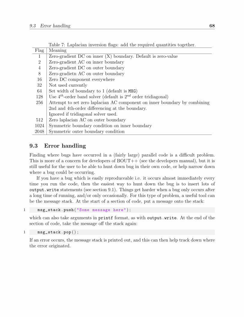
9.3 Error handling 68
Table 7: Laplacian inversion flags: add the required quantities together.Flag Meaning
1 Zero-gradient DC on inner (X) boundary. Default is zero-value2 Zero-gradient AC on inner boundary4 Zero-gradient DC on outer boundary8 Zero-gradietn AC on outer boundary16 Zero DC component everywhere32 Not used currently64 Set width of boundary to 1 (default is MXG)128 Use 4th-order band solver (default is 2nd order tridiagonal)256 Attempt to set zero laplacian AC component on inner boundary by combining
2nd and 4th-order differencing at the boundary.Ignored if tridiagonal solver used.
512 Zero laplacian AC on outer boundary1024 Symmetric boundary condition on inner boundary2048 Symmetric outer boundary condition
9.3 Error handling
Finding where bugs have occurred in a (fairly large) parallel code is a difficult problem.This is more of a concern for developers of BOUT++ (see the developers manual), but it isstill useful for the user to be able to hunt down bug in their own code, or help narrow downwhere a bug could be occurring.
If you have a bug which is easily reproduceable i.e. it occurs almost immediately everytime you run the code, then the easiest way to hunt down the bug is to insert lots ofoutput.write statements (see section 9.1). Things get harder when a bug only occurs aftera long time of running, and/or only occasionally. For this type of problem, a useful tool canbe the message stack. At the start of a section of code, put a message onto the stack:
1 msg_stack . push ("Some message here" ) ;
which can also take arguments in printf format, as with output.write. At the end of thesection of code, take the message off the stack again:
1 msg_stack . pop ( ) ;
If an error occurs, the message stack is printed out, and this can then help track down wherethe error originated.

10. Object-orientated interface 69
10 Object-orientated interface
If you prefer to create classes rather than global variables and C functions for your physicsmodel, this can be done using a (somewhat experimental) interface. To see the difference,compare examples/advect1d/gas compress.cxx withexamples/advect1d-newapi/gas compress.cxx. The disadvantage of this interface isthat it’s marginally more complicated to set up, but it has several advantages: It makessplitting the model into multiple files easier (sharing global variables is a pain), modelscan be combined together to enable coupling of models, and BOUT++ can be more easilyused alongside other libraries. For large models, it’s recommended to use this method.Converting C-style interface to a class is also quite straightforward, and discussed below.
In a header file (e.g. examples/advect1d-newapi/gas compress.hxx), first put
1 #include <bout/ physicsmodel . hxx>
(do NOT include boutmain.hxx, as that defines the C-like interface and a main() function).Next define a class which inherits from PhysicsModel
1 class GasCompress : public PhysicsModel {2 protected :3 int init ( bool restarting ) ;4 int rhs ( BoutReal t ) ;5 private :6 // Evolving v a r i a b l e s , parameters e t c . here7 } ;
As a minimum, you need to define the initialisation function init (it’s a pure virtual memberof PhysicsModel, so if you don’t you’ll get a compile-time error). Any variables being evolvedshould now be members of this class. If you are converting a C-style model, just move allthe global variables into the private section.
Next create a source file (e.g. examples/advect1d-newapi/gas compress.cxx, whichincludes your header file
1 #include "gas_compress.hxx"
Then implement the init and rhs functions:
1 int GasCompress : : init ( bool restarting ) {2 . . .3 }4
5 int GasCompress : : rhs ( BoutReal t ) {6 . . .7 }

11. Differential operators 70
To convert simple physics models, just rename physics_init to YourModel::init, and physics_run←↩to YourModel::run.
Finally, you need to create a main() function for your code. The easiest way to do thisis to use the macro BOUTMAIN:
1 BOUTMAIN ( GasCompress ) ;
This is defined in include/bout/physicsmodel.hxx, and expands to
1 int main ( int argc , char **argv ) {2 BoutInitialise (argc , argv ) ; // I n i t i a l i s e BOUT++3
4 GasCompress *model = new GasCompress ( ) ; // Create a model5
6 Solver *solver = Solver : : create ( ) ; // Create a s o l v e r7 solver−>setModel ( model ) ; // Spec i f y the model to s o l v e8 solver−>addMonitor ( bout_monitor ) ; // Monitor the s o l v e r9
10 solver−>solve ( ) ; // Run the s o l v e r11
12 delete model ;13 delete solver ;14 BoutFinalise ( ) ; // Fin i shed with BOUT++15 return 0 ;16 }
If you like, you can define your own main() function, making it easier to combine BOUT++with other libraries.
11 Differential operators
There are a huge number of possible ways to perform differencing in computational fluiddynamics, and BOUT++ is intended to be able to implement a large number of them. Thismeans that the way differentials are handled internally is quite involved; see the developer’smanual for full gory details. Much of the time this detail is not all that important, andcertainly not while learning to use BOUT++. Default options are therefore set which workmost of the time, so you can start using the code without getting bogged down in thesedetails.
In order to handle many different differencing methods and operations, many layersare used, each of which handles just part of the problem. The main division is betweendifferencing methods (such as 4th-order central differencing), and differential operators (suchas ∇||).

11.1 Differencing methods 71
11.1 Differencing methods
Methods are implemented on 5-point stencils, and are divided into three categories:
� Central-differencing methods, for diffusion operators dfdx
, d2fdx2
. Each method has a shortcode, and currently include
– C2: 2nd order f−1 − 2f0 + f1
– C4: 4th order (−f−2 + 16f−1 − 30f0 + 16f1 − f2) /12
– W2: 2nd order CWENO
– W3: 3rd order CWENO
– FFT: Fourier Transform method in Z (axisymmetric) direction only
� Upwinding methods for advection operators vxdfdx
– U1: 1st order upwinding
– U4: 4th order upwinding
– W3: 3rd order Weighted Essentially Non-Oscillatory (WENO)[?]
� Flux conserving and limiting methods for terms of the form ddx
(vxf)
– SPLIT: split into upwind and central terms ddx
(vxf) = vxdfdx
+ f dvxdx
– NND: Non-oscillatory, containing No free parameters and Dissipative (NND) scheme[?]
Both of these methods avoid overshoots (Gibbs phenomena) at sharp gradients such asshocks, but the simple 1st-order method has very large artificial diffusion. WENO schemesare a development of the ENO reconstruction schemes which combine good handling ofsharp-gradient regions with high accuracy in smooth regions.
To use these differencing operators directly, add the following to the top of your physicsmodule
1 #include <d e r i v s . hxx>
By default the method used will be the one specified in the options input file (see sec-tion 6.7), but most of these methods can take an optional DIFF\_METHOD argument, specifyingexactly which method to use.

11.2 Non-uniform meshes 72
Table 8: Coordinate derivativesFunction FormulaDDX(f) ∂f/∂xDDY(f) ∂f/∂yDDZ(f) ∂f/∂zD2DX2(f) ∂2f/∂x2
D2DY2(f) ∂2f/∂y2
D2DZ2(f) ∂2f/∂z2
D2DX4(f) ∂4f/∂x4
D2DY4(f) ∂4f/∂y4
D2DZ4(f) ∂4f/∂z4
D2DXDZ(f) ∂2f/∂x∂zD2DYDZ(f) ∂2f/∂y∂zVDDX(f, g) f∂g/∂xVDDY(f, g) f∂g/∂yVDDZ(f, g) f∂g/∂zFDDX(f, g) ∂/∂x (f ∗ g)FDDY(f, g) ∂/∂x (f ∗ g)FDDZ(f, g) ∂/∂x (f ∗ g)
11.2 Non-uniform meshes
Setting non uniform = true in the BOUT.inp options file enables corrections to secondderivatives in X and Y . This correction is given by writing derivatives as:
∂f
∂x' 1
∆x
∂f
∂i
where i is the cell index number. The second derivative is therefore given by
∂2f
∂x2' 1
∆x2∂2f
∂i2+
1
∆x
∂f
∂x· ∂∂i
(1
∆x
)The correction factor ∂/∂i (1/∆x) can be calculated automatically, but you can also specifyd2x in the grid file which is
d2x =∂∆x
∂i=∂2x
∂i2
The correction factor is then calculated from d2x using
∂
∂i
(1
∆x
)= − 1
∆x2∂∆x
∂i

11.3 Operators 73
11.3 Operators
These are differential operators which are independent of the coordinate system used.
v = ∇f Vector = Grad(Field)
f = ∇ · a Field = Div(Vector)
v = ∇× a Vector = Curl(Vector)
f = v · ∇g Field = V dot Grad(Vector, Field)
v = a · ∇b Vector = V dot Grad(Vector, Vector)
f = ∇2f Field = Laplacian(Field)
∇φ =∂φ
∂ui∇ui ⇒ (∇φ)i =
∂φ
∂ui
∇ · A = =1
J
∂
∂ui
(JgijAj
)∇2φ = Γi
∂φ
∂ui+ gij
∂2φ
∂ui∂uj
Γi =1
J
∂
∂ui
(Jgij
)Another set of operators assume that the equilibrium magnetic field is written in Clebsh
form as
B0 = ∇z ×∇x |B0| =√gyy
J
Table 9: Clebsch operatorsFunction Formula
Grad par ∂0|| = b0 · ∇ =1√gyy
∂
∂y
Div par ∇0||F = B0∂
0||
(F
B0
)Grad2 par2 ∂2||φ = ∂0||
(∂0||φ
)=
1√gyy
∂
∂y
(1√gyy
)∂φ
∂y+
1
gyy
∂2φ
∂y2
Laplace par ∇2||φ = ∇ · bb · ∇φ =
1
J
∂
∂y
(J
gyy
∂φ
∂y
)Laplace perp ∇2
⊥ = ∇2 −∇2||
Delp2 Perpendicular Laplacian, neglecting all y derivativesThe Laplacian solver performs the inverse operation
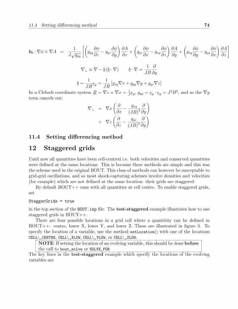
11.4 Setting differencing method 74
b0 · ∇φ×∇A =1
J√gyy
[(gyy
∂φ
∂z− gyz
∂φ
∂y
)∂A
∂x+
(gyz
∂φ
∂x− gxy
∂φ
∂z
)∂A
∂y+
(gxy
∂φ
∂y− gyy
∂φ
∂x
)∂A
∂z
]
∇⊥ ≡ ∇− b (b · ∇) b · ∇ =1
JB
∂
∂y
b =1
JBey =
1
JB[gxy∇x+ gyy∇y + gyz∇z]
In a Clebsch coordinate system B = ∇z ×∇x = 1Jey, gyy = ey · ey = J2B2, and so the ∇y
term cancels out:
∇⊥ = ∇x(∂
∂x− gxy
(JB)2∂
∂y
)
+ ∇z(∂
∂z− gyz
(JB)2∂
∂y
)
11.4 Setting differencing method
12 Staggered grids
Until now all quantities have been cell-centred i.e. both velocities and conserved quantitieswere defined at the same locations. This is because these methods are simple and this wasthe scheme used in the original BOUT. This class of methods can however be susceptable togrid-grid oscillations, and so most shock-capturing schemes involve densities and velocities(for example) which are not defined at the same location: their grids are staggered.
By default BOUT++ runs with all quantities at cell centre. To enable staggered grids,set
StaggerGrids = true
in the top section of the BOUT.inp file. The test-staggered example illustrates how to usestaggered grids in BOUT++.
There are four possible locations in a grid cell where a quantitity can be defined inBOUT++: centre, lower X, lower Y, and lower Z. These are illustrated in figure 3. Tospecify the location of a variable, use the method setLocation() with one of the locationsCELL\_CENTRE, CELL\_XLOW, CELL\_YLOW, or CELL\_ZLOW.
NOTE: If setting the location of an evolving variable, this should be done beforethe call to bout_solve or SOLVE_FOR
The key lines in the test-staggered example which specify the locations of the evolvingvariables are

12. Staggered grids 75
XY
Z
Cell centre
Lower X Lower Y
Lower Z
Figure 3: Locations in a grid cell where quantities may be defined.
1 Field3D n , v ;2
3 int physics_init ( bool restart ) {4 v . setLocation ( CELL_YLOW ) ; // Staggered r e l a t i v e to n5 SOLVE_FOR2 (n , v ) ;6 . . .
which makes the velocity v staggered to the lower side of the cell in Y, whilst the density nremains cell centred.
Arithmetic operations between staggered quantities are handled by interpolating themto the same location according to the algorithm in figure 4. If performing an operationbetween variables defined at two different locations, the order of the variables matter: theresult will be defined at the locations of the left variable. For example, n*v would beCELL_CENTRE because this is the location of n, whilst v*n would be CELL_YLOW. Relying onthis behavior could lead to trouble, to make your code clearer it’s probably best to use theinterpolation routines. Include the header file
1 #include < i n t e r p o l a t i o n . hxx>
then use the interp_to(field, location) function. Using this, interp_to(n, CELL_YLOW)*v
would be CELL_YLOW as n would be interpolated.Differential operators by default return fields which are defined at the same location
as their inputs, so here Grad_par(v) would be CELL_YLOW. If this is not what is wanted,give the location of the result as an additional argument: Grad_par(v, CELL_CENTRE) usesstaggered differencing to produce a result which is defined at the cell centres. As with thearithmetic operators, if you ask for the result to be staggered in a different direction fromthe input then the differencing will be to cell centre and then be interpolated. For example

13. Advanced methods 76
Samelocation?
YesNo interpolation
Samedimensions?
Yes
No
No
Keep first argument
Keep largest
dimension
Figure 4: How the cell location of an arithmetic operation (+,-,*,/,∧ ) is decided
Grad_par(v, CELL_XLOW) would first perform staggered differencing from CELL_YLOW to get aresult at CELL_CENTRE, and then interpolate the result to CELL_XLOW.
Advection operators which take two arguments return a result which is defined at thelocation of the field being advected. For example Vpar_Grad_par(v, f) calculates v∇||f andreturns a result at the same location as f. If v and f are defined at the same locationsthen centred differencing is used, if one is centred and the other staggered then staggereddifferencing is used, and if both are staggered to different locations then the behavior is lesswell defined (don’t do it). As with other differential operators, the required location of theresult can be given as an optional argument.
NOTE: There are subtleties with boundary conditions when staggering variables.The test-staggered example manually applies a boundary condition to make thewidth of the boundary wider
13 Advanced methods
This section describes the more advanced methods which can be used to speed up simulationsusing implicit time stepping schemes. At the time of writing (Dec ’12), they can be usedwith either the SUNDIALS CVODE or PETSc solvers.
13.1 Preconditioning
At every time step, an implicit scheme such as BDF has to solve a nonlinear problem to findthe next solution. This is usually done using Newton’s method, each step of which involves
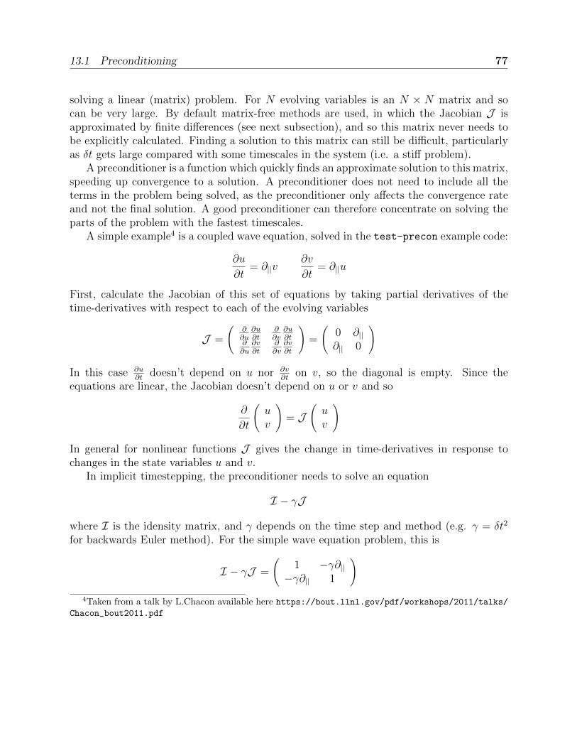
13.1 Preconditioning 77
solving a linear (matrix) problem. For N evolving variables is an N × N matrix and socan be very large. By default matrix-free methods are used, in which the Jacobian J isapproximated by finite differences (see next subsection), and so this matrix never needs tobe explicitly calculated. Finding a solution to this matrix can still be difficult, particularlyas δt gets large compared with some timescales in the system (i.e. a stiff problem).
A preconditioner is a function which quickly finds an approximate solution to this matrix,speeding up convergence to a solution. A preconditioner does not need to include all theterms in the problem being solved, as the preconditioner only affects the convergence rateand not the final solution. A good preconditioner can therefore concentrate on solving theparts of the problem with the fastest timescales.
A simple example4 is a coupled wave equation, solved in the test-precon example code:
∂u
∂t= ∂||v
∂v
∂t= ∂||u
First, calculate the Jacobian of this set of equations by taking partial derivatives of thetime-derivatives with respect to each of the evolving variables
J =
(∂∂u
∂u∂t
∂∂v
∂u∂t
∂∂u
∂v∂t
∂∂v
∂v∂t
)=
(0 ∂||∂|| 0
)
In this case ∂u∂t
doesn’t depend on u nor ∂v∂t
on v, so the diagonal is empty. Since theequations are linear, the Jacobian doesn’t depend on u or v and so
∂
∂t
(uv
)= J
(uv
)
In general for nonlinear functions J gives the change in time-derivatives in response tochanges in the state variables u and v.
In implicit timestepping, the preconditioner needs to solve an equation
I − γJ
where I is the idensity matrix, and γ depends on the time step and method (e.g. γ = δt2
for backwards Euler method). For the simple wave equation problem, this is
I − γJ =
(1 −γ∂||−γ∂|| 1
)4Taken from a talk by L.Chacon available here https://bout.llnl.gov/pdf/workshops/2011/talks/
Chacon_bout2011.pdf

13.1 Preconditioning 78
This matrix can be block inverted using Schur factorisation5
(E UL D
)−1=
(I −E−1U0 I
)(E−1 0
0 P−1Schur
)(I 0
−LE−1 I
)
where PSchur = D− LE−1U Using this, the wave problem becomes:
(1 −γ∂||−γ∂|| 1
)−1=
(1 γ∂||0 1
) 1 0
0(1− γ2∂2||
)−1( 1 0
γ∂|| 1
)(1)
The preconditioner is implemented by defining a function of the form
int precon ( BoutReal t , BoutReal gamma , BoutReal delta ) {. . .
}which takes as input the current time, the γ factor appearing above, and δ which is onlyimportant for constrained problems (not discussed here... yet). The current state of thesystem is stored in the state variables (here u and v), whilst the vector to be preconditionedis stored in the time derivatives (here ddt(u) and ddt(v)). At the end of the preconditionerthe result should be in the time derivatives. A preconditioner which is just the identitymatrix and so does nothing is therefore:
int precon ( BoutReal t , BoutReal gamma , BoutReal delta ) {}
NOTE: This changed in github/bendudson on 15th Aug 2014. In older versionsthe result must be returned in the state variables
To implement the preconditioner in equation 1, first apply the rightmost matrix to thegiven vector: (
ddt(u)
ddt(v)
)=
(1 0γ∂|| 1
)(ddt(u)
ddt(v)
)
int precon ( BoutReal t , BoutReal gamma , BoutReal delta ) {mesh−>communicate ( ddt (u ) ) ;// ddt (u) = ddt (u) ;ddt (v ) = gamma*Grad_par ( ddt (u ) ) + ddt (v ) ;
note that since the preconditioner is linear, it doesn’t depend on u or v. As in the RHSfunction, since we are taking a differential of ddt(u), it first needs to be communicated toexchange guard cell values.
5See paper http://arxiv.org/abs/1209.2054 for an application to 2-fluid equations

13.1 Preconditioning 79
The second matrix(ddt(u)
ddt(v)
)← 1 0
0(1− γ2∂2||
)−1( ddt(u)
ddt(v)
)
doesn’t alter u, but solves a parabolic equation in the parallel direction. There is a solverclass to do this called InvertPar which solves the equation
(A+B∂2||
)x = b where A and
B are Field2D or constants6. In physics_init we create one of these solvers:
InvertPar *inv ; // P a r a l l e l i n v e r s i o n c l a s sint physics_init ( bool restarting ) {
. . .inv = InvertPar : : Create ( ) ;inv−>setCoefA ( 1 . 0 ) ;. . .
}In the preconditioner we then use this solver to update v:
inv−>setCoefB(−SQ ( gamma ) ) ;ddt (v ) = inv−>solve ( ddt (v ) ) ;
which solves ddt(v)←(1− γ2∂2||
)−1ddt(v). The final matrix just updates u using this new
solution for v (ddt(u)
ddt(v)
)←(
1 γ∂||0 1
)(ddt(u)
ddt(v)
)
mesh−>communicate ( ddt (v ) ) ;ddt (u ) = ddt (u ) + gamma*Grad_par ( ddt (v ) ) ;
Finally, boundary conditions need to be imposed, which should be consistent with theconditions used in the RHS
ddt (u ) . applyBoundary ("dirichlet" ) ;ddt (v ) . applyBoundary ("dirichlet" ) ;
To use the preconditioner, pass the function to the solver in physics_init
1 int physics_init ( bool restarting ) {2 solver−>setPrecon ( precon ) ;3 . . .4 }
6This InvertPar class can handle cases with closed field-lines and twist-shift boundary conditions fortokamak simulations

13.2 Jacobian function 80
then in the BOUT.inp settings file switch on the preconditioner
[ solver ]type = cvode # Need CVODE or PETScuse_precon = true # Use p r e c o n d i t i o n e rrightprec = false # Use Right p r e c o n d i t i o n e r ( d e f a u l t l e f t )
13.2 Jacobian function
13.3 DAE constraint equations
Using the IDA solver, BOUT++ can solve Differential Algebraic Equations (DAEs), inwhich algebraic constraints are used for some variables.
13.4 Monitoring the simulation output
At every output timestep the solver calls a monitor function, which writes the output dumpfile, calculates and prints timing information and estimated time remaining. If you want torun additional code or write data to a different file, you can add monitor function(s).
You can call your monitor function whatever you like, but it must have 4 inputs andreturn an int:
1 int my_monitor ( Solver *solver , BoutReal simtime , int iter , int NOUT ) ←↩{
2 . . .3 }
The first input is the solver object, the second is the current simulation time, the thirdis the output number, and the last is the total number of outputs requested. To get thesolver to call this function every output time, put in your physics\_init code:
1 solver−>addMonitor ( my_monitor ) ;
If you want to later remove a monitor, you can do so with
1 solver−>removeMonitor ( my_monitor ) ;
A simple example using this monitor is:
1 int my_monitor ( Solver *solver , BoutReal simtime , int iter , int NOUT ) ←↩{
2 output . write ("My monitor, time = %e, dt = %e\n" ,3 simtime , solver−>getCurrentTimestep ( ) ) ;4 }5
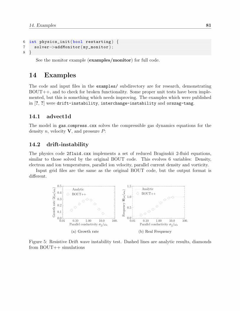
14. Examples 81
6 int physics_init ( bool restarting ) {7 solver−>addMonitor ( my_monitor ) ;8 }
See the monitor example (examples/monitor) for full code.
14 Examples
The code and input files in the examples/ subdirectory are for research, demonstratingBOUT++, and to check for broken functionality. Some proper unit tests have been imple-mented, but this is something which needs improving. The examples which were publishedin [?, ?] were drift-instability, interchange-instability and orszag-tang.
14.1 advect1d
The model in gas compress.cxx solves the compressible gas dynamics equations for thedensity n, velocity V, and pressure P :
14.2 drift-instability
The physics code 2fluid.cxx implements a set of reduced Braginskii 2-fluid equations,similar to those solved by the original BOUT code. This evolves 6 variables: Density,electron and ion temperatures, parallel ion velocity, parallel current density and vorticity.
Input grid files are the same as the original BOUT code, but the output format isdifferent.
Growth
rate=(ω/ω∗) Analytic
BOUT++
0.0
0.1
0.2
0.3
0.4
0.5
Parallel conductivity σ||/ω∗0.01 0.10 1.00 10.0 100.
(a) Growth rate
Parallel conductivity σ||/ω∗0.01 0.10 1.00 10.0 100.
Frequency<(ω/ω∗)
0.0
0.5
1.0
1.5Analytic
BOUT++
(b) Real Frequency
Figure 5: Resistive Drift wave instability test. Dashed lines are analytic results, diamondsfrom BOUT++ simulations

14.3 em-drift 82
14.3 em-drift
14.4 gyro-gem
14.5 interchange-instability
0 20 40 60 80 100 120
106
104
102
100
10−2
10−4
10−6
R = 1 m
R = 10 m
Time [µs]
RMSdensity〈n〉
Figure 6: Interchange instability test. Solid lines are from analytic theory, symbols fromBOUT++ simulations, and the RMS density is averaged over z. Vertical dashed line marksthe reference point, where analytic and simulation results are set equal
14.6 jorek-compare
14.7 lapd-drift
14.8 orszag-tang
The file mhd.cxx solves the full MHD equations for the full values (perturbation + initial),whilst the file mhd perturb.cxx solves for a perturbation about the equilibrium.

14.9 shear-alfven-wave 83
Figure 7: Sod shock-tube problem for testing shock-handling methods
14.9 shear-alfven-wave
14.10 sod-shock
14.11 uedge-benchmark
15 Notes
15.1 Compile options
Compiling with -DCHECK enables a lot of checks of operations performed by the field objects.This is very useful for debugging a code, and can be omitted once bugs have been removed.
For (sometimes) more useful error messages, there is the -DTRACK option. This keepstrack of the names of variables and includes these in error messages.
15.2 Adaptive grids
Two types of adaptive grids can be used in BOUT++: Moving meshes, and changingresolution.
15.2.1 Moving meshes
During either the initialisation, or the simulation itself, the metric tensors can be modified.This could be used to make the coordinate system time-dependent. Since currently themetric tensors are 2D fields, this would only allow axi-symmetric motion. Changing thetensors to be 3D objects is however possible with fairly small modification to the code.

REFERENCES 84
Whenever one of the metrics gij are changed, a call to geometry() must be made.
15.2.2 Changing resolution
NOTE: Not implemented yet - this just for discussion
Since all 2D and 3D fields/vectors are located internally in global lists, the resolutionof the grid can be changed when required by interpolation. This requires a new, moreefficient implementation of the Fields classes.
References
[1] B.D. Dudson, M.V. Umansky, X.Q. Xu, P.B. Snyder, and H.R. Wilson. Bout++: Aframework for parallel plasma fluid simulations. Computer Physics Communications, InPress, Corrected Proof:–, 2009.
[2] B D Dudson, M V Umansky, X Q Xu, P B Snyder, and H R Wilson. BOUT++: aframework for parallel plasma fluid simulations. arXiv, physics.plasm-ph:0810.5757, Nov2008.
[3] M V Umansky, X Q Xu, B Dudson, and L L LoDestro. BOUT Code Manual. LLNL,June 2006. Available from www.mfescience.org/bout/.
[4] M V Umansky, X Q Xu, B Dudson, L L LoDestro, and J R Myra. Statusand verification of edge plasma turbulence code bout. Comp. Phys. Comm., pagedoi:10.1016/j.cpc.2008.12.012, 2008.
[5] X Q Xu, M V Umansky, B Dudson, and P B Snyder. Boundary plasma turbulencesimulations for tokamaks. Comm. in Comput. Phys., 4(5):pp. 949–979, November 2008.
[6] W H Press, S A Teukolsky, W T Vetterling, and B P Flannery. Numerical recipes in C.The art of scientific computing. Cambridge University Press, 1999.
[7] Guang-Shan Jiang and Danping Peng. Weighted ENO schemes for Hamilton-Jacobiequations. SIAM J. Sci. Comp., 21(6):2126–2143, 2000.
[8] F Chen, A Xu, G Zhang, and Y Li. Three-dimensional lattice boltzmann model forhigh-speed compressible flows. arXiv, page 1010.4135v1, 2010.
A Installing PACT
There are two ways to install PACT, and usually one of them will work on a given system.

A.1 Self-extracting package 85
A.1 Self-extracting package
This is probably the easiest method (when it works). Download one of the “ExecutableUNIX distribution files” from the PACT website and run:
./pact07_07_18-src -sl -i $HOME/local/
The “-sl” flag tells it to generate shared libraries. If you don’t plan on using IDL toread/write PDB files, then you can omit this. The “-i $HOME/local/” tells PACT toinstall in your home directory/local.
If this script fails, you will usually have to resort to either trying to understand DSYS,or going with the second method below.
A.2 PACT source distribution
The second method is to use a .tar.gz PACT source file. Here the version used is pact-2.1.0.tar.gz.
~/ $ cd install
~/install/ $ tar -xzvf pact-2.1.0.tar.gz
~/install/ $ cd pact-2.1.0/
~/install/pact-2.1.0/ $ ./configure --prefix=$HOME/local --enable-shared
NOTE: On Franklin, PACT will compile without the –enable-shared option, butnot with it. This is OK if you just want to run BOUT++, but the shared librariesare needed for reading the results into IDL (the PDB2IDL library)
At this point, the installation may fail with the following error:
configure: WARNING: yacc is a symbolic link to bison
configure: WARNING: bison is not a supported type of yacc
configure: error: No working yacc found
If this happens, you need to first install Berkeley Yacc into your home directory
~/install/ $ ls
byacc.tar.gz netcdf-tar -xzvf byacc.tar.gz4.0.1.tar.gz pact-2.1.0.tar.gz
fftw-3.2.1.tar.gz pact-2.1.0 sundials-2.4.0.tar.gz
~/install/ $ tar -xzvf byacc.tar.gz
~/install/ $ cd byacc-20080826/
~/install/byacc-20080826/ $ ./configure --prefix=$HOME/local
~/install/byacc-20080826/ $ gmake
~/install/byacc-20080826/ $ mkdir ~/local/bin
~/install/byacc-20080826/ $ cp yacc ~/local/bin/
B. Compiling and running under AIX 86
NB: We’re copying the yacc executable manually because “gmake install” doesn’t seem towork, and the fix which works for PACT (see later) doesn’t work here.
Add this directory to your path:
~/install/byacc-20080826/ $ setenv PATH $HOME/local/bin:$PATH
You can check that this has worked by running “which yacc”, which should then print yourhome directory /local/bin/yacc. You could also add this to your .profile startup scripts.Now go back to PACT:
~/install/byacc-20080826/ $ cd ../pact-2.1.0
~/install/pact-2.1.0/ $ ./configure --prefix=$HOME/local --enable-shared
~/install/pact-2.1.0/ $ gmake
~/install/pact-2.1.0/ $ gmake install
The last step may fail with a strange error message like:
The current directory must be set to the ITT directory.
Change the default to the ITT directory and re-run
this script.
This happens when the wrong “install” is being used. Check by running:
~/install/byacc-20080826/ $ which install
This should print “/usr/bin/install”, but if not then run
~/install/byacc-20080826/ $ ln -s /usr/bin/install ~/local/bin/
~/install/pact-2.1.0/ $ ./configure --prefix=$HOME/local
~/install/pact-2.1.0/ $ gmake
~/install/pact-2.1.0/ $ gmake install
NOTE: configure needs to be run again after messing with install.This should now install PACT into your local directory.
B Compiling and running under AIX
Most development and running of BOUT++ is done under Linux, with the occasionalFreeBSD and OSX. The configuration scripts are therefore heavily tested on these architec-tures. IBM’s POWER architecture however runs AIX, which has some crucial differenceswhich make compiling a pain.
B.1 SUNDIALS 87
� Under Linux/BSD, it’s usual for a Fortran routine foo to appear under C as foo ,whilst under AIX the name is unchanged
� MPI compiler scripts are usually given the names mpicc and either mpiCC or mpicxx.AIX uses mpcc and mpCC.
� Like BSD, the make command isn’t compatible with GNU make, so you have to rungmake to compile everything.
� The POWER architecture is big-endian, different to the little endian Intel and AMDchips. This can cause problems with binary file formats.
B.1 SUNDIALS
To compile SUNDIALS, use
$ export CC=cc
$ export CXX=xlC
$ export F77=xlf
$ export OBJECT_MODE=64
$ ./configure --prefix=$HOME/local/ --with-mpicc=mpcc --with-mpif77=mpxlf CFLAGS=-maix64
You may get an error message like:
make: Not a recognized flag: w
This is because the AIX make is being used, rather than gmake. The easiest way to fix thisis to make a link to gmake in your local bin directory:
$ ln -s /usr/bin/gmake $HOME/local/bin/make
Running which make should now point to this local/bin/make, and if not then you needto make sure that your bin directory appears first in the PATH:
export PATH=$HOME/local/bin:$PATH
If you see an error like this:
ar: 0707-126 ../../src/sundials/sundials_math.o is not valid with the current object file mode.
Use the -X option to specify the desired object mode.
then you need to set the environment variable OBJECT MODE
export OBJECT_MODE=64

C. BOUT++ functions (alphabetical) 88
Configuring BOUT++, you may get the error:
configure: error: C compiler cannot create executables
In that case, you can try using:
./configure CFLAGS="-maix64"
When compiling, you may see warnings
xlC_r: 1501-216 (W) command option -64 is not recognized - passed to ld
At this point, the main BOUT++ library should compile, and you can try compilingone of the examples.
ld: 0711-317 ERROR: Undefined symbol: .NcError::NcError(NcError::Behavior)
ld: 0711-317 ERROR: Undefined symbol: .NcFile::is_valid() const
ld: 0711-317 ERROR: Undefined symbol: .NcError::~NcError()
ld: 0711-317 ERROR: Undefined symbol: .NcFile::get_dim(const char*) const
This is probably because the NetCDF libraries are 32-bit, whilst BOUT++ has beencompiled as 64-bit. You can try compiling BOUT++ as 32-bit:
$ export OBJECT_MODE=32
$ ./configure CFLAGS="-maix32"
$ gmake
If you still get undefined symbols, then go back to 64-bit, and edit make.config, raplacing-lnetcdf c++ with -lnetcdf64 c++, and -lnetcdf with -lnetcdf64. This can be done byrunning:
$ sed ’s/netcdf/netcdf64/g’ make.config > make.config.new
$ mv make.config.new make.config
C BOUT++ functions (alphabetical)
This is a list of functions which can be called by users writing a physics module. For a fulllist of functions, see the Reference manual, DOxygen documentation, and source code.
� Field = abs(Field | Vector)
� (Communicator).add(Field | Vector)
Add a variable to a communicator object.

C. BOUT++ functions (alphabetical) 89
� apply boundary(Field. ‘‘name’’)
� Field = b0xGrad dot Grad(Field, Field, CELL LOC)
� bout solve(Field, Field, ‘‘name’’)
� bout solve(Vector, Vector, ‘‘name’’)
� (Communicator).clear()Remove all variables from a Communicator object
� Field = cos(Field)
� Field = cosh(Field)
� Vector = Curl(Vector)
� Field = Delp2(Field)∇2⊥ operator
� Field = Div(Vector)Divergence of a vector
� Field = Div par(Field f)
Parallel divergence B0b · ∇ (f/B0)
� dump.add(Field, ‘‘name’’, 1/0)
� Field = filter(Field, modenr)
� geometry derivs()Calculates useful quantities from the metric tensor. Call this every time the metrictensor is changed.
� Vector = Grad(Field)
� Field = Grad par(Field)
� Field = Grad2 par2(Field)
� grid load(BoutReal, ‘‘name’’)
Load a scalar real from the grid file
� grid load2d(Field2D, ‘‘name’’)
Load a 2D scalar field from the grid file

C. BOUT++ functions (alphabetical) 90
� grid load3d(Field3D, ‘‘name’’)
Load a 3D scalar field from the grid file
� invert laplace(Field input, Field output, flags, Field2D *A)
� Field = invert parderiv(Field2D|BoutReal A, Field2D|BoutReal B, Field3D r)
Inverts an equation A*x + B*Grad2 par2(x) = r
� Field = Laplacian(Field)
� Field3D = low pass(Field3D, max modenr)
� BoutReal = max(Field)
� BoutReal = min(Field)
� msg stack.pop( |int)
Remove a message from the top of the stack. If a message ID is passed, removes allmessages back to that point.
� int = msg stack.push(‘‘format’’, ...)
Put a message onto the stack. Works like printf (and output.write).
� options.get(‘‘name’’, variable, default)
Get an integer, real or boolean value from the options file. If not in the file, the defaultvalue is used. The value used is printed to log file.
� options.setSection(‘‘name’’) Set the section name in the input file
� output << values
Behaves like cout for stream output
� output.write(‘‘format’’, ...)
Behaves like printf for formatted output
� (Communicator).receive()Receive data from other processors. Must be preceded by a send call.
� (Communicator).run()Sends and receives data.
� (Communicator).send()Sends data to other processors (and posts receives). This must be followed by a callto receive() before calling send again, or adding new variables.
D. IDL routines 91
� (Field3D).setLocation(CELL LOC)
� (Field3D).ShiftZ(bool)
� Field = sin(Field)
� Field = sinh(Field)
� solver.setPrecon(PhysicsPrecon)Set a preconditioner function
� Field = sqrt(Field)
� Field = tan(Field)
� Field = tanh(Field)
� Field = V dot Grad(Vector v, Field f)
Calculates an advection term v · ∇f
� Vector = V dot Grad(Vector v, Vector u)
Advection term v · ∇u
� Field = Vpar Grad par(Field v, Field f)
� Field3D = where(Field2D test, Field|BoutReal gt0, Field|BoutReal lt0)
Chooses between two values, depending on sign of test.
D IDL routines
List of IDL routines available in idllib. There are broadly three categories of routine:
� Completely general routines which could be useful outside BOUT++ work
– Data plotting and animation: contour2 and showdata
– File reading and writing: file open, file read etc.
– User input and output: get float, get integer, get yesno and str
– FFT routines for integrating, differentiating and filtering: fft integrate, fft deriv,fft filter
� Routines for BOUT++, but not specific to any application
– Modifying restart files: expand restarts, scale restarts and split restarts

D. IDL routines 92
– Processing 3D variables for input grid: bout3dvar
� Routines specifically for tokamak simulations
– Reading A- and G-EQDSK format files into IDL: read aeqdsk and read neqdsk
– Plotting results: polslice, plotpolslice
Here the format isname, arguments, [optional arguments]
� var = bout3dvar ( var )Converts 3D variables to and from BOUT++’s Fourier representation which is usedfor input grids. By default converts from [x,y,z] to [x,y,f]
– /reverse Convert from [x,y,f] to [x,y,z]
– nf=nf Set number of frequencies in the result
– nz=nz When using /reverse, set number of Z points in the result
� var = collect()Read in data from a set of BOUT++ dump files
– var = “name of variable”
– path = “path/to/variable/”
– xind, yind, zind, tind = [min, max] index pairs
– t array = Output 1D array of times
� contour2, data [, x, y]This is a replacement for the IDL contour which includes a scale color bar.
– data can be either 2D (x,y) or 3D (x,y,t). If data is 3D then the color is scaledto the entire range.
– x is an optional 2D (x,y) array of X coordinates
– y is an optional 2D (x,y) array of Y coordinates
– t=t is a time index for 3D data
– nlev=nlev
– centre=centre Make zero the middle of the color range (white if redblue)
– redblue=redblue Use a blue-white-red color scheme
– revcolor=revcolor Reverse color scheme

D. IDL routines 93
� expand restarts, newzIncreases the number of Z points in restart files. Together with scale restarts andsplit restarts, this makes it easier to modify a linear simulation as a start for nonlinearruns.
– newz is the new value of NZ
– path=path Input path
– output=output Output path
– format=format File extension of output
� result = fft deriv ( var1d )Calculates the derivative of a variable on a periodic domain.
� result = fft filter (var, nf) Fourier filter a variable on a periodic domain. Argumentsare a 1D variable and the number of Fourier components to keep
� result = fft integrate ( var1d ) Integrates a variable on a periodic domain.
– loop=loop The loop integral is returned in this variable
� file close, handleClose a file opened using file open()
� list = file list ( handle )Return a list of variable names in the file
� integer = file ndims ( handle , “variable” )Get the number of dimensions of a variable
� handle = file open ( “file” )Open a PDB or NetCDF file. File type is inferred from file name
– /write Open file for writing (default is read only)
– /create Create a new file, over-writing if already exists
� var = file read ( handle, “variable” )
– inds = [xmin, xmax, ymin, ymax, ... ]
� float = get float ( “prompt” )Ask the user for a float, using the given prompt
D. IDL routines 94
� integer = get integer ( “prompt” )Ask the user for an integer
� integer = get yesno ( “prompt” )Ask for a yes (1) or no (0) answer
� result = gmres ( x0, operator, b )General Minimal Residual (GMRES)
– x0 is the starting guess at the solution
– operator
– b
Optional arguments
– restart=restart
– max iter=max iter
– tol=tol
– stats=stats
– show=show
– output=output
� result = int func ( [x,] f )Integrate a function, always using the maximum number of grid-points possible forhighest accuracy
� bool = is pow2 ( value )Returns 1 (true) if the given number is a power of 2, 0 (false) otherwise
� plotpolslice, var3d, gridTakes a slice through a field-aligned tokamak domain, showing a poloidal cross-section.
– var3d is a 3D (x,y,z) variable to plot. Needs all of the points to work properly.
– grid is a structure from importing a grid file
Optional arguments:
– period=period
– zangle=zangle
– nlev=nlev
D. IDL routines 95
– yr=yr
– profile=profile
– output=output
– lines=lines
– linecol=linecol
– filter=filter
� polslice, data, gridfilePlots a 2D poloidal contour for single or double-null configurations, including colorbar.
– xstart=xstart X index where the data begins. Useful if only part of the domainhas been collected
– ystart=ystart Y index where data begins
� struct = read aeqdsk ( ”filename” )Reads an A-EQDSK file. Format is specified here: https://fusion.gat.com/THEORY/efit/a_eqdsk.html
� struct = read neqdsk ( ”filename” )Reads in an ’neqdsk’ or G-EQDSK formatted tokamak equilibrium file. Format ofG-EQDSK file is specified here: https://fusion.gat.com/THEORY/efit/g_eqdsk.
html
� stringarray = regex extract ( line, pattern )Extract all matches to Regular Expression pattern contained in line. Useful for ex-tracting numbers from FORTRAN-formatted text files.
– line Input string
– pattern Regular expression pattern to match
– nmatch=nmatch
� var = reverse inds ( var )Reverse array indices e.g. arr[t,z,y,x] -> arr[x,y,z,t]. Works on up to 5 di-mensional variables
� safe colorsSets the color table to useful values for plotting.
– /first Sets the first 10 colors to specific values, otherwise sets last 7

D. IDL routines 96
� scale restarts, factor
– path=path Path to the restart files (default is current directory ’.’)
– format=format Specify what the file format is, otherwise goes on the file name
� showdata, dataDisplay animations of 1D,2D and 3D data. Defaults:
– 2D data Animate a line plot
– 3D data Animate a surface plot
– 4D data Animate a poloidal cross-section (tokamaks only)
Optional arguments:
– /addsym For 2D data (1D plots), add symbols to mark data points
– az=angle Rotate surface plots
– /bw Make contour plots greyscale
– chars=size character size
– /contour For 3D input, show color contour plot
– delay=time Time delay between plots (default 0.2 seconds)
– /noscale By default, all plots are on the same scale. This changes the scale foreach plot’s range
– profile=array Background profile. Data is 3D: profile is 1D (X). Data is 4D -¿profile is 2D (X,Y)
– yr=[min,max] Y range
� result = sign ( var )This returns +1 if the variable is > 0, -1 otherwise
� spectrum
� split restarts, [nxpe], nypesplit restart files between a different number of processors
– nxpe is an optional argument giving the number of processors in the X direction
– nype is the number of processors in the Y direction
– path=path Input path
– output=output Output path

E. Python routines (alphabetical) 97
– format=format File extension of output
� string = str ( value )Convert a value to a string with whitespace trimmed. Arrays are converted to acomma-separated list in brackets.
� result = zfamp ( var4d )Given a 4D variable [x,y,z,t], returns the Fourier amplitudes in [x,y,f,t]
� var = zshift ( var, shift )Shifts a variable in the Z direction, useful for mapping between field-aligned andorthogonal coordinates.
– period=period How many domains fit in 2π. Default is 1 (full torus)
E Python routines (alphabetical)
E.1 boututils
� class Datafile provides a convenient way to read and write NetCDF files. There aremany different NetCDF libraries available for Python, so this class tries to provide aconsistent interface to many of them.
� deriv()
� determineNumberOfCPUs()
� file_import() reads the contents of a NetCDF file into a dictionary
� integrate()
� launch()
� linear_regression()
E.2 boutdata
� collect() provides an interface to read BOUT++ data outputs, returning NumPyarrays of data. It deals with the processor layout, working out which file containseach part of the domain.
1 from boutdata import collect
2
3 t = collect ("t_array" ) # Collect the time values

E.2 boutdata 98
� pol_slice() takes a 3 or 4-D data set for a toroidal equilibrium, and calculates a slicethrough it at fixed toroidal angle.
� gen_surface() is a generator for iterating over flux surfaces

Index
boundary conditions, 40, 57Boundary modifiers, 41BoutReal, 52
Clebsh, 70comm handle, 57Command line, 32communication, 36, 55cvode.cxx, 14
differencing, 36, 68dskgato, 47
EFIT, 45ELITE, 47Expressions, 38
Field3D, 52FieldFactory, 38FieldGroup, 55function, 38
GATO, 47Github, 4GRID LOAD, 61
Hypnotoad, 45
IDL, 25
Laplacian inversion, 36, 63
metric tensor, 44msg stack, 65
non-uniform mesh, 69
Options, 54options, 31output, 63
PACT, 81Python, 29
SAVE ONCE, 61SOLVE FOR, 53staggered grids, 71Symmetric initial conditions, 39
time integration, 34
variable initialisation, 37, 60Vector3D, 52
99


![GOME Data Processor Extraction Software User’s Manualwdc.dlr.de/sensors/gome/user_manual.pdf · 2009. 7. 28. · by ESA [G1], and was launched on 21 April 1995 on board the second](https://img.pdfslide.net/doc/110x75/6072fb3997118e244c5320dd/gome-data-processor-extraction-software-useras-2009-7-28-by-esa-g1-and.jpg)