Brain4Cars: Car That Knows Before You Dovia Sensory-Fusion Deep Learning ArchitectureAshesh Jain1,2, Hema S Koppula1,2, Shane Soh2, Bharad Raghavan2, Avi Singh1, and Ashutosh Saxena3

Cornell University1, Stanford University2, Brain Of Things Inc.3

{ashesh,hema}@cs.cornell.edu, avisingh@iitk.ac.in, {shanesoh,bharadr,asaxena}@cs.stanford.edu

Abstract—Advanced Driver Assistance Systems (ADAS) havemade driving safer over the last decade. They prepare vehiclesfor unsafe road conditions and alert drivers if they perform adangerous maneuver. However, many accidents are unavoidablebecause by the time drivers are alerted, it is already too late.Anticipating maneuvers beforehand can alert drivers before theyperform the maneuver and also give ADAS more time to avoidor prepare for the danger.

In this work we propose a vehicular sensor-rich platform andlearning algorithms for maneuver anticipation. For this purposewe equip a car with cameras, Global Positioning System (GPS),and a computing device to capture the driving context from bothinside and outside of the car. In order to anticipate maneuvers,we propose a sensory-fusion deep learning architecture whichjointly learns to anticipate and fuse multiple sensory streams.Our architecture consists of Recurrent Neural Networks (RNNs)that use Long Short-Term Memory (LSTM) units to capture longtemporal dependencies. We propose a novel training procedurewhich allows the network to predict the future given only apartial temporal context. We introduce a diverse data set with1180 miles of natural freeway and city driving, and show that wecan anticipate maneuvers 3.5 seconds before they occur in real-time with a precision and recall of 90.5% and 87.4% respectively.

I. INTRODUCTION

Over the last decade cars have been equipped with variousassistive technologies in order to provide a safe driving experi-ence. Technologies such as lane keeping, blind spot check, pre-crash systems etc., are successful in alerting drivers wheneverthey commit a dangerous maneuver [43]. Still in the US alonemore than 33,000 people die in road accidents every year, themajority of which are due to inappropriate maneuvers [2]. Wetherefore need mechanisms that can alert drivers before theyperform a dangerous maneuver in order to avert many suchaccidents [56].

In this work we address the problem of anticipating maneu-vers that a driver is likely to perform in the next few seconds.Figure 1 shows our system anticipating a left turn maneuver afew seconds before the car reaches the intersection. Our systemalso outputs probabilities over the maneuvers the driver canperform. With this prior knowledge of maneuvers, the driverassistance systems can alert drivers about possible dangersbefore they perform the maneuver, thereby giving them moretime to react. Some previous works [22, 41, 50] also predicta driver’s future maneuver. However, as we show in thefollowing sections, these methods use limited context and/ordo not accurately model the anticipation problem.

0.1

0.2

0.7

Face Camera

Road Camera

Fig. 1: Anticipating maneuvers. Our algorithm anticipates drivingmaneuvers performed a few seconds in the future. It uses informationfrom multiple sources including videos, vehicle dynamics, GPS, andstreet maps to anticipate the probability of different future maneuvers.

In order to anticipate maneuvers, we reason with the contex-tual information from the surrounding events, which we referto as the driving context. We obtain this driving context frommultiple sources. We use videos of the driver inside the carand the road in front, the vehicle’s dynamics, global positioncoordinates (GPS), and street maps; from this we extract a timeseries of multi-modal data from both inside and outside thevehicle. The challenge lies in modeling the temporal aspects ofdriving and fusing the multiple sensory streams. In this workwe propose a specially tailored approach for anticipation insuch sensory-rich settings.

Anticipation of the future actions of a human is an importantperception task with applications in robotics and computervision [39, 77, 33, 34, 73]. It requires the prediction of futureevents from a limited temporal context. This differentiatesanticipation from activity recognition [73], where the completetemporal context is available for prediction. Furthermore,in sensory-rich robotics settings like ours, the context foranticipation comes from multiple sensors. In such scenariosthe end performance of the application largely depends onhow the information from different sensors are fused. Previousworks on anticipation [33, 34, 39] usually deal with single-data modality and do not address anticipation for sensory-richrobotics applications. Additionally, they learn representationsusing shallow architectures [30, 33, 34, 39] that cannot handlelong temporal dependencies [6].

In order to address the anticipation problem more generally,

arX

iv:1

601.

0074

0v1

[cs

.RO

] 5

Jan

201

6

𝐱2𝐱1 𝐱3 𝐱𝑇

𝐲 𝐲 𝐲 𝐲

(𝐱1, 𝐱2, … , 𝐱𝑇) → 𝐲

Training example

Training RNN for anticipation

𝐱1 𝐱𝑡

𝐲𝑡

(𝐱1, 𝐱2, … , 𝐱𝑡)

Test example

Anticipation given partial context

?

1 𝑇 1 𝑡𝑡 =

Fig. 2: (Left) Shows training RNN for anticipation in a sequence-to-sequence prediction manner. The network explicitly learns to mapthe partial context (x1, ..,xt) ∀t to the future event y. (Right) Attest time the network’s goal is to anticipate the future event as soonas possible, i.e. by observing only a partial temporal context.

we propose a Recurrent Neural Network (RNN) based archi-tecture which learns rich representations for anticipation. Wefocus on sensory-rich robotics applications, and our architec-ture learns how to optimally fuse information from differentsensors. Our approach captures temporal dependencies byusing Long Short-Term Memory (LSTM) units. We trainour architecture in a sequence-to-sequence prediction manner(Figure 2) such that it explicitly learns to anticipate given apartial context, and we introduce a novel loss layer whichhelps anticipation by preventing over-fitting.

We evaluate our approach on a driving data set with 1180miles of natural freeway and city driving collected acrosstwo states – from 10 drivers and with different kinds ofdriving maneuvers. The data set is challenging because ofthe variations in routes and traffic conditions, and the drivingstyles of the drivers (Figure 3). We demonstrate that our deeplearning sensory-fusion approach anticipates maneuvers 3.5seconds before they occur with 84.5% precision and 77.1%recall while using out-of-the-box face tracker. With moresophesticated 3D pose estimation of the face, our precisionand recall increases to 90.5% and 87.4% respectively. Webelieve that our work creates scope for new ADAS featuresto make roads safer. In summary our key contributions are asfollows:

• We propose an approach for anticipating driving maneu-vers several seconds in advance.

• We propose a generic sensory-fusion RNN-LSTM archi-tecture for anticipation in robotics applications.

• We release the first data set of natural driving with videosfrom both inside and outside the car, GPS, and speedinformation.

• We release an open-source deep learning package

Fig. 3: Variations in the data set. Images from the data set [30]for a left lane change. (Left) Views from the road facing camera.(Right) Driving style of the drivers vary for the same maneuver.

NeuralModels which is especially designed forrobotics applications with multiple sensory streams.

Our data set and deep learning code are publicly available at:http://www.brain4cars.com

II. RELATED WORK

Our work builds upon the previous works on assisitivevehicular technologies, anticipating human activities, learningtemporal models, and computer vision methods for analyzinghuman face.Assistive features for vehicles. Latest cars available in marketcomes equipped with cameras and sensors to monitor thesurrounding environment. Through multi-sensory fusion theyprovide assisitive features like lane keeping, forward collisionavoidance, adaptive cruise control etc. These systems warndrivers when they perform a potentially dangerous maneu-ver [59, 68]. Driver monitoring for distraction and drowsinesshas also been extensively researched [21, 55]. Techniqueslike eye-gaze tracking are now commercially available (SeeingMachines Ltd.) and has been effective in detecting distraction.Our work complements existing ADAS and driver monitoringtechniques by anticipating maneuvers several seconds beforethey occur.

Closely related to us are previous works on predicting thedriver’s intent. Vehicle trajectory has been used to predictthe intent for lane change or turn maneuver [9, 22, 41, 44].Most of these works ignore the rich context available fromcameras, GPS, and street maps. Previous works have ad-dressed maneuver anticipation [1, 50, 15, 67] through sensory-fusion from multiple cameras, GPS, and vehicle dynamics.In particular, Morris et al. [50] and Trivedi et al. [67] usedRelevance Vector Machine (RVM) for intent prediction andperformed sensory fusion by concatenating feature vectors. Wewill show that such hand designed concatenation of featuresdoes not work well. Furthermore, these works do not modelthe temporal aspect of the problem properly. They assume

that informative contextual cues always appear at a fixedtime before the maneuver. We show that this assumption isnot true, and in fact the temporal aspect of the problemshould be carefully modeled. In contrast to these works, ourRNN-LSTM based sensory-fusion architecture captures longtemporal dependencies through its memory cell and learnsrich representations for anticipation through a hierarchy ofnon-linear transformations of input data. Our work is alsorelated to works on driver behavior prediction with differentsensors [26, 21, 20], and vehicular controllers which act onthese predictions [59, 68, 18].Anticipation and Modeling Humans. Modeling of humanmotion has given rise to many applications, anticipation beingone of them. Anticipating human activities has shown toimprove human-robot collaboration [73, 36, 46, 38, 16]. Sim-ilarly, forecasting human navigation trajectories has enabledrobots to plan sociable trajectories around humans [33, 8,39, 29]. Feature matching techniques have been proposedfor anticipating human activities from videos [57]. Modelinghuman preferences has enabled robots to plan good trajecto-ries [17, 60, 28, 31]. Similar to these works, we anticipatehuman actions, which are driving maneuvers in our case.However, the algorithms proposed in the previous works donot apply in our setting. In our case, anticipating maneuversrequires modeling the interaction between the driving contextand the driver’s intention. Such interactions are absent in theprevious works, and they use shallow architectures [6] thatdo not properly model temporal aspects of human activities.They further deal with a single data modality and do not tacklethe challenges of sensory-fusion. Our problem setup involvesall these challenges, for which we propose a deep learningapproach which efficiently handles temporal dependencies andlearns to fuse multiple sensory streams.Analyzing the human face. The vision approaches related toour work are face detection and tracking [69, 76], statisticalmodels of face [10] and pose estimation methods for face [75].Active Appearance Model (AAM) [10] and its variants [47, 74]statistically model the shape and texture of the face. AAMshave also been used to estimate the 3D-pose of a face froma single image [75] and in design of assistive features fordriver monitoring [55, 63]. In our approach we adapt off-the-shelf available face detection [69] and tracking algorithms [58](see Section VI). Our approach allows us to easily experimentwith more advanced face detection and tracking algorithms.We demonstrate this by using the Constrained Local NeuralField (CLNF) model [4] and tracking 68 fixed landmark pointson the driver’s face and estimating the 3D head-pose.Learning temporal models. Temporal models are commonlyused to model human activities [35, 49, 71, 72]. These modelshave been used in both discriminative and generative fashions.The discriminative temporal models are mostly inspired bythe Conditional Random Field (CRF) [42] which capturesthe temporal structure of the problem. Wang et al. [72]and Morency et al. [49] propose dynamic extensions ofthe CRF for image segmentation and gesture recognitionrespectively. On the other hand, generative approaches for

temporal modeling include various filtering methods, suchas Kalman and particle filters [64], Hidden Markov Models,and many types of Dynamic Bayesian Networks [51]. Someprevious works [9, 40, 53] used HMMs to model differentaspects of the driver’s behaviour. Most of these generativeapproaches model how latent (hidden) states influence theobservations. However, in our problem both the latent statesand the observations influence each other. In the followingsections, we will describe the Autoregressive Input-OutputHMM (AIO-HMM) for maneuver anticipation [30] and willuse it as a baseline to compare our deep learning approach.Unlike AIO-HMM our deep architecture have internal memorywhich allows it to handle long temporal dependencies [24].Furthermore, the input features undergo a hierarchy of non-linear transformation through the deep architecture whichallows learning rich representations.

Two building blocks of our architecture are RecurrentNeural Networks (RNNs) [54] and Long Short-Term Memory(LSTM) units [25]. Our work draws upon ideas from pre-vious works on RNNs and LSTM from the language [62],speech [23], and vision [14] communities. Our approach to thejoint training of multiple RNNs is related to the recent workon hierarchical RNNs [19]. We consider RNNs in multi-modalsetting, which is related to the recent use of RNNs in image-captioning [14]. Our contribution lies in formulating activityanticipation in a deep learning framework using RNNs withLSTM units. We focus on sensory-rich robotics applications,and our architecture extends previous works doing sensory-fusion with feed-forward networks [52, 61] to the fusion oftemporal streams. Using our architecture we demonstrate state-of-the-art on maneuver anticipation.

III. OVERVIEW

We first give an overview of the maneuver anticipationproblem and then describe our system.

A. Problem Overview

Our goal is to anticipate driving maneuvers a few secondsbefore they occur. This includes anticipating a lane changebefore the wheels touch the lane markings or anticipating ifthe driver keeps straight or makes a turn when approachingan intersection. This is a challenging problem for multiplereasons. First, it requires the modeling of context from dif-ferent sources. Information from a single source, such as acamera capturing events outside the car, is not sufficiently rich.Additional visual information from within the car can also beused. For example, the driver’s head movements are useful foranticipation – drivers typically check for the side traffic whilechanging lanes and scan the cross traffic at intersections.

Second, reasoning about maneuvers should take into ac-count the driving context at both local and global levels. Localcontext requires modeling events in vehicle’s vicinity such asthe surrounding vision, GPS, and speed information. On theother hand, factors that influence the overall route contributesto the global context, such as the driver’s final destination.Third, the informative cues necessary for anticipation appear at

.31

.07

.74

1

Input: Videos, GPS

Speed & Maps

1

0

(a) Setup

Face detection &

Tracking feature points Motion of facial points

(c) Inside and Outside Vehicle Features (d) Model (e) Anticipation(b) Vision Algorithms

Outside context

Feature

vector

Road camera

Face camera

t=0t=5

LSTM

Networks

Fusion

Layer

Softmax

Inside

FeaturesOutside

Features

Fig. 4: System Overview. Our system anticipating a left lane change maneuver. (a) We process multi-modal data including GPS, speed,street maps, and events inside and outside of the vehicle using video cameras. (b) Vision pipeline extracts visual cues such as driver’s headmovements. (c) The inside and outside driving context is processed to extract expressive features. (d,e) Using our deep learning architecturewe fuse the information from outside and inside the vehicle and anticipate the probability of each maneuver.

t=1

t=5

t=4 t=2

t=3

t=0

Left lane change

Right lane change

Right turn Trajectories of

facial points

x y

Fig. 5: Variable time occurrence of events. Left: The events insidethe vehicle before the maneuvers. We track the driver’s face alongwith many facial points. Right: The trajectories generated by thehorizontal motion of facial points (pixels) ‘t’ seconds before themaneuver. X-axis is the time and Y-axis is the pixels’ horizontalcoordinates. Informative cues appear during the shaded time interval.Such cues occur at variable times before the maneuver, and the orderin which the cues appear is also important.

variable times before the maneuver, as illustrated in Figure 5.In particular, the time interval between the driver’s headmovement and the occurrence of the maneuver depends onmany factors such as the speed, traffic conditions, etc.

In addition, appropriately fusing the information from mul-tiple sensors is crucial for anticipation. Simple sensory fusionapproaches like concatenation of feature vectors performspoorly, as we demonstrate through experiments. In our pro-posed approach we learn a neural network layer for fusingthe temporal streams of data coming from different sensors.Our resulting architecture is end-to-end trainable via backpropagation, and we jointly train it to: (i) model the temporalaspects of the problem; (ii) fuse multiple sensory streams; and(iii) anticipate maneuvers.

B. System Overview

For maneuver anticipation our vehicular sensory platformincludes the following (as shown in Figure 4):

1) A driver-facing camera inside the vehicle. We mount thiscamera on the dashboard and use it to track the driver’shead movements. This camera operates at 25 fps.

2) A camera facing the road is mounted on the dash-board to capture the (outside) view in front of the car.This camera operates at 30 fps. The video from thiscamera enables additional reasoning on maneuvers. Forexample, when the vehicle is in the left-most lane,the only safe maneuvers are a right-lane change orkeeping straight, unless the vehicle is approaching anintersection.

3) A speed logger for vehicle dynamics because maneuverscorrelate with the vehicle’s speed, e.g., turns usuallyhappen at lower speeds than lane changes.

4) A Global Positioning System (GPS) for localizing thevehicle on the map. This enables us to detect upcomingroad artifacts such as intersections, highway exits, etc.

Using this system we collect 1180 miles of natural cityand freeway driving data from 10 drivers. We denote theinformation from sensors with feature vector x. Our vehic-ular systems gives a temporal sequence of feature vectors{(x1,x2, ...,xt, ...)}. For now we do not distinguish betweenthe information from different sensors, later in Section V-Bwe introduce sensory fusion. In Section VI we formallydefine our feature representations and describe our data setin Section VIII-A. We now formally define anticipation andpresent our deep learning architecture.

IV. PRELIMINARIES

We now formally define anticipation and then present ourRecurrent Neural Network architecture. The goal of anticipa-tion is to predict an event several seconds before it happensgiven the contextual information up to the present time.The future event can be one of multiple possibilities. Attraining time a set of temporal sequences of observations andevents {(x1,x2, ...,xT )j ,yj}Nj=1 is provided where xt is theobservation at time t, y is the representation of the event

(described below) that happens at the end of the sequence att = T , and j is the sequence index. At test time, however, thealgorithm receives an observation xt at each time step, andits goal is to predict the future event as early as possible,i.e. by observing only a partial sequence of observations{(x1, ...,xt)|t < T}. This differentiates anticipation fromactivity recognition [70, 37] where in the latter the completeobservation sequence is available at test time. In this paper,xt is a real-valued feature vector and y = [y1, ..., yK ] is avector of size K (the number of events), where yk denotesthe probability of the temporal sequence belonging to eventthe k such that

∑Kk=1 y

k = 1. At the time of training, y takesthe form of a one-hot vector with the entry in y correspondingto the ground truth event as 1 and the rest 0.

In this work we propose a deep RNN architecture withLong Short-Term Memory (LSTM) units [25] for anticipation.Below we give an overview of the standard RNN and LSTMwhich form the building blocks of our architecture.

A. Recurrent Neural Networks

A standard RNN [54] takes in a temporal sequence ofvectors (x1,x2, ...,xT ) as input, and outputs a sequenceof vectors (h1,h2, ...,hT ) also known as high-level repre-sentations. The representations are generated by non-lineartransformation of the input sequence from t = 1 to T , asdescribed in the equations below.

ht = f(Wxt + Hht−1 + b) (1)yt = softmax(Wyht + by) (2)

where f is a non-linear function applied element-wise, and ytis the softmax probabilities of the events having seen the ob-servations up to xt. W, H, b, Wy , by are the parameters thatare learned. Matrices are denoted with bold, capital letters, andvectors are denoted with bold, lower-case letters. In a standardRNN a common choice for f is tanh or sigmoid. RNNswith this choice of f suffer from a well-studied problem ofvanishing gradients [54], and hence are poor at capturing longtemporal dependencies which are essential for anticipation. Acommon remedy to vanishing gradients is to replace tanhnon-linearities by Long Short-Term Memory cells [25]. Wenow give an overview of LSTM and then describe our modelfor anticipation.

B. Long-Short Term Memory Cells

LSTM is a network of neurons that implements a memorycell [25]. The central idea behind LSTM is that the memorycell can maintain its state over time. When combined withRNN, LSTM units allow the recurrent network to rememberlong term context dependencies.

LSTM consists of three gates – input gate i, output gateo, and forget gate f – and a memory cell c. See Figure 6for an illustration. At each time step t, LSTM first computesits gates’ activations {it,ft} (3)(4) and updates its memorycell from ct−1 to ct (5), it then computes the output gateactivation ot (6), and finally outputs a hidden representationht (7). The inputs into LSTM are the observations xt and

Fig. 6: Internal working of an LSTM unit.

the hidden representation from the previous time step ht−1.LSTM applies the following set of update operations:

it = σ(Wixt + Uiht−1 + Vict−1 + bi) (3)ft = σ(Wfxt + Ufht−1 + Vfct−1 + bf ) (4)ct = ft � ct−1 + it � tanh(Wcxt + Ucht−1 + bc) (5)ot = σ(Woxt + Uoht−1 + Voct + bo) (6)ht = ot � tanh(ct) (7)

where � is an element-wise product and σ is the logisticfunction. σ and tanh are applied element-wise. W∗, V∗, U∗,and b∗ are the parameters, further the weight matrices V∗ arediagonal. The input and forget gates of LSTM participate inupdating the memory cell (5). More specifically, forget gatecontrols the part of memory to forget, and the input gatecomputes new values based on the current observation thatare written to the memory cell. The output gate together withthe memory cell computes the hidden representation (7). SinceLSTM cell activation involves summation over time (5) andderivatives distribute over sums, the gradient in LSTM getspropagated over a longer time before vanishing. In the standardRNN, we replace the non-linear f in equation (1) by theLSTM equations given above in order to capture long temporaldependencies. We use the following shorthand notation todenote the recurrent LSTM operation.

(ht, ct) = LSTM(xt,ht−1, ct−1) (8)

We now describe our RNN architecture with LSTM unitsfor anticipation. Following which we will describe a particularinstantiation of our architecture for maneuver anticipationwhere the observations x come from multiple sources.

V. NETWORK ARCHITECTURE FOR ANTICIPATION

In order to anticipate, an algorithm must learn to predictthe future given only a partial temporal context. This makesanticipation challenging and also differentiates it from activityrecognition. Previous works treat anticipation as a recognitionproblem [34, 50, 57] and train discriminative classifiers (suchas SVM or CRF) on the complete temporal context. However,at test time these classifiers only observe a partial temporalcontext and make predictions within a filtering framework. Wemodel anticipation with a recurrent architecture which unfoldsthrough time. This lets us train a single classifier that learnsto handle partial temporal context of varying lengths.

Furthermore, anticipation in robotics applications is chal-lenging because the contextual information can come frommultiple sensors with different data modalities. Examplesinclude autonomous vehicles that reason from multiple sen-sors [3] or robots that jointly reason over perception andlanguage instructions [48]. In such applications the way infor-mation from different sensors is fused is critical to the appli-cation’s final performance. We therefore build an end-to-enddeep learning architecture which jointly learns to anticipateand fuse information from different sensors.

A. RNN with LSTM units for anticipation

At the time of training, we observe the complete tempo-ral observation sequence and the event {(x1,x2, ...,xT ),y}.Our goal is to train a network which predicts the fu-ture event given a partial temporal observation sequence{(x1,x2, ...,xt)|t < T}. We do so by training an RNN in asequence-to-sequence prediction manner. Given training exam-ples {(x1,x2, ...,xT )j ,yj}Nj=1 we train an RNN with LSTMunits to map the sequence of observations (x1,x2, ...,xT ) tothe sequence of events (y1, ...,yT ) such that yt = y,∀t,as shown in Fig. 2. Trained in this manner, our RNNwill attempt to map all sequences of partial observations(x1,x2, ...,xt) ∀t ≤ T to the future event y. This wayour model explicitly learns to anticipate. We additionally useLSTM units which prevents the gradients from vanishing andallows our model to capture long temporal dependencies inhuman activities.1

B. Fusion-RNN: Sensory fusion RNN for anticipation

We now present an instantiation of our RNN architecturefor fusing two sensory streams: {(x1, ...,xT ), (z1, ..., zT )}. Inthe next section we will describe these streams for maneuveranticipation.

An obvious way to allow sensory fusion in the RNN is byconcatenating the streams, i.e. using ([x1; z1], ..., [xT ; zT ]) asinput to the RNN. However, we found that this sort of simpleconcatenation performs poorly. We instead learn a sensoryfusion layer which combines the high-level representations ofsensor data. Our proposed architecture first passes the twosensory streams {(x1, ...,xT ), (z1, ..., zT )} independentlythrough separate RNNs (9) and (10). The high level repre-sentations from both RNNs {(hx1 , ...,hxT ), (hz1, ...,h

zT ) are

then concatenated at each time step t and passed through afully connected (fusion) layer which fuses the two represen-tations (11), as shown in Figure 7. The output representationfrom the fusion layer is then passed to the softmax layer foranticipation (12). The following operations are performed fromt = 1 to T .

(hxt , cxt ) = LSTMx(xt,h

xt−1, c

xt−1) (9)

(hzt , czt ) = LSTMz(zt,h

zt−1, c

zt−1) (10)

Sensory fusion: et = tanh(Wf [hxt ;h

zt ] + bf ) (11)

yt = softmax(Wyet + by) (12)

1Driving maneuvers can take up to 6 seconds and the value of T can goup to 150 with a camera frame rate of 25 fps.

LSTM LSTM LSTM

𝐱𝑡𝐱𝑡−1 𝐱𝑡+1

LSTM LSTM LSTM

𝐳𝑡𝐳𝑡−1 𝐳𝑡+1

𝐲𝑡−1 𝐲𝑡 𝐲𝑡+1

Fusion

Layer

Softmax

Exponentially

growing loss

Predictions

𝑙𝑜𝑠𝑠 = −∑𝑒− 𝑇−𝑡 log(y𝑡𝑘 )

Fig. 7: Sensory fusion RNN for anticipation. (Bottom) In theFusion-RNN each sensory stream is passed through their independentRNN. (Middle) High-level representations from RNNs are thencombined through a fusion layer. (Top) In order to prevent over-fitting early in time the loss exponentially increases with time.

where W∗ and b∗ are model parameters, and LSTMx

and LSTMz process the sensory streams (x1, ...,xT ) and(z1, ..., zT ) respectively. The same framework can be extendedto handle more sensory streams.

C. Exponential loss-layer for anticipation.

We propose a new loss layer which encourages the architec-ture to anticipate early while also ensuring that the architecturedoes not over-fit the training data early enough in time whenthere is not enough context for anticipation. When usingthe standard softmax loss, the architecture suffers a loss of− log(ykt ) for the mistakes it makes at each time step, whereykt is the probability of the ground truth event k computedby the architecture using Eq. (12). We propose to modify thisloss by multiplying it with an exponential term as illustratedin Figure 7. Under this new scheme, the loss exponentiallygrows with time as shown below.

loss =

N∑j=1

T∑t=1

−e−(T−t) log(ykt ) (13)

This loss penalizes the RNN exponentially more for the mis-takes it makes as it sees more observations. This encouragesthe model to fix mistakes as early as it can in time. The loss inequation 13 also penalizes the network less on mistakes madeearly in time when there is not enough context available. Thisway it acts like a regularizer and reduces the risk to over-fitvery early in time.

VI. FEATURES

We extract features by processing the inside and outsidedriving contexts. We do this by grouping the overall contextualinformation from the sensors into: (i) the context from insidethe vehicle, which comes from the driver facing camera and isrepresented as temporal sequence of features (z1, ..., zT ); and(ii) the context from outside the vehicle, which comes fromthe remaining sensors: GPS, road facing camera, and street

t=0t=2t=3t=5

0

0.9T

raje

cto

ries

Angula

r m

otion

Angle

His

togra

m

Fig. 8: Inside vehicle feature extraction. The angular histogramfeatures extracted at three different time steps for a left turn maneuver.Bottom: Trajectories for the horizontal motion of tracked facial pixels‘t’ seconds before the maneuver. At t=5 seconds before the maneuverthe driver is looking straight, at t=3 looks (left) in the directionof maneuver, and at t=2 looks (right) in opposite direction for thecrossing traffic. Middle: Average motion vector of tracked facialpixels in polar coordinates. r is the average movement of pixels andarrow indicates the direction in which the face moves when lookingfrom the camera. Top: Normalized angular histogram features.

maps. We represent the outside context with (x1, ...,xT ). Inorder to anticipate maneuvers, our RNN architecture (Figure 7)processes the temporal context {(x1, ...,xt), (z1, ..., zt)} atevery time step t, and outputs softmax probabilities yt for thefollowing five maneuvers:M = {left turn, right turn, left lanechange, right lane change, straight driving}.

A. Inside-vehicle features.

The inside features zt capture the driver’s head movementsat each time instant t. Our vision pipeline consists of facedetection, tracking, and feature extraction modules. We extracthead motion features per-frame, denoted by φ(face). Wecompute zt by aggregating φ(face) for every 20 frames, i.e.,zt =

∑20i=1 φ(facei)/‖

∑20i=1 φ(facei)‖.

Face detection and tracking. We detect the driver’s face using atrained Viola-Jones face detector [69]. From the detected face,we first extract visually discriminative (facial) points using theShi-Tomasi corner detector [58] and then track those facialpoints using the Kanade-Lucas-Tomasi (KLT) tracker [45, 58,66]. However, the tracking may accumulate errors over timebecause of changes in illumination due to the shadows of trees,traffic, etc. We therefore constrain the tracked facial points tofollow a projective transformation and remove the incorrectlytracked points using the RANSAC algorithm. While trackingthe facial points, we lose some of the tracked points withevery new frame. To address this problem, we re-initialize thetracker with new discriminative facial points once the numberof tracked points falls below a threshold [32].

t=5

t=5

t=0

t=0

(a) Features using KLT Tracker 2D Trajectories

(b) Features using CLNF Tracker 2D Trajectories

Fig. 9: Improved features for maneuver anticipation. We trackfacial landmark points using the CLNF tracker [4] which results inmore consistent 2D trajectories as compared to the KLT tracker [58]used by Jain et al. [30]. Furthermore, the CLNF also gives an estimateof the driver’s 3D head pose.

Head motion features. For maneuver anticipation the hori-zontal movement of the face and its angular rotation (yaw)are particularly important. From the face tracking we ob-tain face tracks, which are 2D trajectories of the trackedfacial points in the image plane. Figure 8 (bottom) showshow the horizontal coordinates of the tracked facial pointsvary with time before a left turn maneuver. We representthe driver’s face movements and rotations with histogramfeatures. In particular, we take matching facial points betweensuccessive frames and create histograms of their correspondinghorizontal motions (in pixels) and angular motions in theimage plane (Figure 8). We bin the horizontal and angularmotions using [≤ −2, −2 to 0, 0 to 2, ≥ 2] and[0 to π

2 ,π2 to π, π to 3π

2 ,3π2 to 2π], respectively. We also

calculate the mean movement of the driver’s face center. Thisgives us φ(face) ∈ R9 facial features per-frame. The driver’seye-gaze is also useful a feature. However, robustly estimating3D eye-gaze in outside environment is still a topic of research,and orthogonal to this work on anticipation. We therefore donot consider eye-gaze features.3D head pose and facial landmark features. Our framework isflexible and allows incorporating more advanced face detectionand tracking algorithms. For example we replace the KLTtracker described above with the Constrained Local NeuralField (CLNF) model [4] and track 68 fixed landmark points onthe driver’s face. CLNF is particularly well suited for drivingscenarios due its ability to handle a wide range of head poseand illumination variations. As shown in Figure 9, CLNFoffers us two distinct benefits over the features from KLT (i)while discriminative facial points may change from situation tosituation, tracking fixed landmarks results in consistent opticalflow trajectories which adds to robustness; and (ii) CLNF alsoallows us to estimate the 3D head pose of the driver’s faceby minimizing error in the projection of a generic 3D meshmodel of the face w.r.t. the 2D location of landmarks in theimage. The histogram features generated from the optical flowtrajectories along with the 3D head pose features (yaw, pitchand row), give us φ(face) ∈ R12 when using the CLNF tracker.

x1

h1

z1

x2

ℎ2

z2

x3

z3

ℎ3 ℎ𝑇

z𝑇

x𝑇

𝑇

?

Input

Layer

Hidden

Layer

Output

Layer

Inside features

Outside features

Driver states

Fig. 10: AIO-HMM. The model has three layers: (i) Input (top):this layer represents outside vehicle features x; (ii) Hidden (middle):this layer represents driver’s latent states h; and (iii) Output (bottom):this layer represents inside vehicle features z. This layer also capturestemporal dependencies of inside vehicle features. T represents time.

In Section VIII we present results with the features fromKLT, as well as the results with richer features obtained fromthe CLNF model.

B. Outside-vehicle features.

The outside feature vector xt encodes the informationabout the outside environment such as the road conditions,vehicle dynamics, etc. In order to get this information, weuse the road-facing camera together with the vehicle’s GPScoordinates, its speed, and the street maps. More specifically,we obtain two binary features from the road-facing cameraindicating whether a lane exists on the left side and on theright side of the vehicle. We also augment the vehicle’s GPScoordinates with the street maps and extract a binary featureindicating if the vehicle is within 15 meters of a road artifactsuch as intersections, turns, highway exists, etc. We alsoencode the average, maximum, and minimum speeds of thevehicle over the last 5 seconds as features. This results in axt ∈ R6 dimensional feature vector.

VII. BAYESIAN NETWORKS FORMANEUVER ANTICIPATION

In this section we propose alternate Bayesian networks [30]based on Hidden Markov Model (HMM) for maneuver antic-ipation. These models form a strong baseline to compare oursensory-fusion deep learning architecture.

Driving maneuvers are influenced by multiple interactionsinvolving the vehicle, its driver, outside traffic, and occa-sionally global factors like the driver’s destination. Theseinteractions influence the driver’s intention, i.e. their state ofmind before the maneuver, which is not directly observable. Inour Bayesian network formulation, we represent the driver’sintention with discrete states that are latent (or hidden). Inorder to anticipate maneuvers, we jointly model the drivingcontext and the latent states in a tractable manner. We rep-resent the driving context as a set of features described inSection VI. We now present the motivation for the Bayesiannetworks and then discuss our key model AutoregressiveInput-Output HMM (AIO-HMM).

Fig. 11: Our data set is diverse in drivers and landscape.

A. Modeling driving maneuvers

Modeling maneuvers require temporal modeling of thedriving context. Discriminative methods, such as the SupportVector Machine and the Relevance Vector Machine [65],which do not model the temporal aspect perform poorly onanticipation tasks, as we show in Section VIII. Therefore, atemporal model such as the Hidden Markov Model (HMM) isbetter suited to model maneuver anticipation.

An HMM models how the driver’s latent states generateboth the inside driving context (zt) and the outside drivingcontext (xt). However, a more accurate model should capturehow events outside the vehicle (i.e. the outside driving context)affect the driver’s state of mind, which then generates theobservations inside the vehicle (i.e. the inside driving context).Such interactions can be modeled by an Input-Output HMM(IOHMM) [7]. However, modeling the problem with IOHMMdoes not capture the temporal dependencies of the insidedriving context. These dependencies are critical to capturethe smooth and temporally correlated behaviours such as thedriver’s face movements. We therefore present AutoregressiveInput-Output HMM (AIO-HMM) which extends IOHMM tomodel these observation dependencies. Figure 10 shows theAIO-HMM graphical model for modeling maneuvers. Welearn separate AIO-HMM model for each maneuver. In orderto anticipate maneuvers, during inference we determine whichmodel best explains the past several seconds of the drivingcontext based on the data log-likelihood. In Appendix A wedescribe the training and inference procedure for AIO-HMM.

VIII. EXPERIMENTS

In this section we first give an overview of our dataset and then present the quantitative results. We alsodemonstrate our system and algorithm on real-world driv-ing scenarios. Our video demonstrations are available at:http://www.brain4cars.com.

A. Driving data set

Our data set consists of natural driving videos with bothinside and outside views of the car, its speed, and the globalposition system (GPS) coordinates.2 The outside car video

2The inside and outside cameras operate at 25 and 30 frames/sec.

captures the view of the road ahead. We collected this drivingdata set under fully natural settings without any intervention.3

It consists of 1180 miles of freeway and city driving andencloses 21,000 square miles across two states. We collectedthis data set from 10 drivers over a period of two months. Thecomplete data set has a total of 2 million video frames andincludes diverse landscapes. Figure 11 shows a few samplesfrom our data set. We annotated the driving videos with atotal of 700 events containing 274 lane changes, 131 turns,and 295 randomly sampled instances of driving straight. Eachlane change or turn annotation marks the start time of themaneuver, i.e., before the car touches the lane or yaws,respectively. For all annotated events, we also annotated thelane information, i.e., the number of lanes on the road and thecurrent lane of the car. Our data set is publicly available athttp://www.brain4cars.com.

B. Baseline algorithms

We compare the following algorithms:

• Chance: Uniformly randomly anticipates a maneuver.• SVM [50]: Support Vector Machine is a discriminative

classifier [11]. Morris et al. [50] takes this approach foranticipating maneuvers.4 We train the SVM on 5 secondsof driving context by concatenating all frame features toget a R3840 dimensional feature vector.

• Random-Forest [12]: This is also a discriminative classi-fier that learns many decision trees from the training data,and at test time it averages the prediction of the individualdecision trees. We train it on the same features as SVMwith 150 trees of depth ten each.

• HMM: This is the Hidden Markov Model. We train theHMM on a temporal sequence of feature vectors that weextract every 0.8 seconds, i.e., every 20 video frames.We consider three versions of the HMM: (i) HMM E:with only outside features from the road camera, thevehicle’s speed, GPS and street maps (Section VI-B); (ii)HMM F : with only inside features from the driver’s face(Section VI-A); and (ii) HMM E + F : with both insideand outside features.

• IOHMM: Jain et al. [30] modeled driving maneuvers withthis Bayesian network. It is trained on the same featuresas HMM E + F .

• AIO-HMM: Jain et al. [30] proposed this Bayesian net-work for modeling maneuvers. It is trained on the samefeatures as HMM E + F .

• Simple-RNN (S-RNN): In this architecture sensor streamsare fused by simple concatenation and then passedthrough a single RNN with LSTM units.

• Fusion-RNN-Uniform-Loss (F-RNN-UL): In this archi-tecture sensor streams are passed through separate RNNs,

3Protocol: We set up cameras, GPS and speed recording device in subject’spersonal vehicles and left it to record the data. The subjects were asked toignore our setup and drive as they would normally.

4Morries et al. [50] considered binary classification problem (lane changevs driving straight) and used RVM [65].

Algorithm 1 Maneuver anticipation

Initialize m∗ = driving straightInput Features {(x1, ...,xT ), (z1, ..., zT )} and predictionthreshold pthOutput Predicted maneuver m∗

while t = 1 to T doObserve features (x1, ...,xt) and (z1, ..., zt)Estimate probability yt of each maneuver in Mm∗t = argmaxm∈M ytif m∗t 6= driving straight & yt{m∗t } > pth thenm∗ = m∗tbreak

end ifend whileReturn m∗

and the high-level representations from RNNs are thenfused via a fully-connected layer. The loss at each timestep takes the form − log(ykt ).

• Fusion-RNN-Exp-Loss (F-RNN-EL): This architecture issimilar to F-RNN-UL, except that the loss exponentiallygrows with time −e−(T−t) log(ykt ).

Our RNN and LSTM implementations are open-sourcedand available at NeuralModels [27]. For the RNNs in ourFusion-RNN architecture we use a single layer LSTM of size64 with sigmoid gate activations and tanh activation for hiddenrepresentation. Our fully connected fusion layer uses tanhactivation and outputs a 64 dimensional vector. Our overallarchitecture (F-RNN-EL and F-RNN-UL) have nearly 25,000parameters that are learned using RMSprop [13].

C. Evaluation protocol

We evaluate an algorithm based on its correctness in pre-dicting future maneuvers. We anticipate maneuvers every 0.8seconds where the algorithm processes the recent contextand assigns a probability to each of the four maneuvers:{left lane change, right lane change, left turn, right turn}and a probability to the event of driving straight. These fiveprobabilities together sum to one. After anticipation, i.e. whenthe algorithm has computed all five probabilities, the algorithmpredicts a maneuver if its probability is above a thresholdpth. If none of the maneuvers’ probabilities are above thisthreshold, the algorithm does not make a maneuver predictionand predicts driving straight. However, when it predicts oneof the four maneuvers, it sticks with this prediction andmakes no further predictions for next 5 seconds or until amaneuver occurs, whichever happens earlier. After 5 secondsor a maneuver has occurred, it returns to anticipating futuremaneuvers. Algorithm 1 shows the inference steps for maneu-ver anticipation.

During this process of anticipation and prediction, thealgorithm makes (i) true predictions (tp): when it predicts thecorrect maneuver; (ii) false predictions (fp): when it predictsa maneuver but the driver performs a different maneuver; (iii)false positive predictions (fpp): when it predicts a maneuver

TABLE I: Maneuver Anticipation Results. Average precision, recall and time-to-maneuver are computed from 5-fold cross-validation.Standard error is also shown. Algorithms are compared on the features from Jain et al. [30].

Lane change Turns All maneuvers

Method Pr (%) Re (%) Time-to-Pr (%) Re (%) Time-to-

Pr (%) Re (%) Time-to-maneuver (s) maneuver (s) maneuver (s)

Chance 33.3 33.3 - 33.3 33.3 - 20.0 20.0 -Morris et al. [50] SVM 73.7 ± 3.4 57.8 ± 2.8 2.40 64.7 ± 6.5 47.2 ± 7.6 2.40 43.7 ± 2.4 37.7 ± 1.8 1.20

Random-Forest 71.2 ± 2.4 53.4 ± 3.2 3.00 68.6 ± 3.5 44.4 ± 3.5 1.20 51.9 ± 1.6 27.7 ± 1.1 1.20HMM E 75.0 ± 2.2 60.4 ± 5.7 3.46 74.4 ± 0.5 66.6 ± 3.0 4.04 63.9 ± 2.6 60.2 ± 4.2 3.26HMM F 76.4 ± 1.4 75.2 ± 1.6 3.62 75.6 ± 2.7 60.1 ± 1.7 3.58 64.2 ± 1.5 36.8 ± 1.3 2.61

HMM E + F 80.9 ± 0.9 79.6 ± 1.3 3.61 73.5 ± 2.2 75.3 ± 3.1 4.53 67.8 ± 2.0 67.7 ± 2.5 3.72IOHMM 81.6 ± 1.0 79.6 ± 1.9 3.98 77.6 ± 3.3 75.9 ± 2.5 4.42 74.2 ± 1.7 71.2 ± 1.6 3.83

(Our final Bayesian network) AIO-HMM 83.8 ± 1.3 79.2 ± 2.9 3.80 80.8 ± 3.4 75.2 ± 2.4 4.16 77.4 ± 2.3 71.2 ± 1.3 3.53S-RNN 85.4 ± 0.7 86.0 ± 1.4 3.53 75.2 ± 1.4 75.3 ± 2.1 3.68 78.0 ± 1.5 71.1 ± 1.0 3.15

F-RNN-UL 92.7 ± 2.1 84.4 ± 2.8 3.46 81.2 ± 3.5 78.6 ± 2.8 3.94 82.2 ± 1.0 75.9 ± 1.5 3.75(Our final deep architecture) F-RNN-EL 88.2 ± 1.4 86.0 ± 0.7 3.42 83.8 ± 2.1 79.9 ± 3.5 3.78 84.5 ± 1.0 77.1 ± 1.3 3.58

but the driver does not perform any maneuver (i.e. drivingstraight); and (iv) missed predictions (mp): when it predictsdriving straight but the driver performs a maneuver. Weevaluate the algorithms using their precision and recall scores:

Pr =tp

tp+ fp+ fpp︸ ︷︷ ︸Total # of maneuver predictions

; Re =tp

tp+ fp+mp︸ ︷︷ ︸Total # of maneuvers

The precision measures the fraction of the predicted maneu-vers that are correct and recall measures the fraction of the ma-neuvers that are correctly predicted. For true predictions (tp)we also compute the average time-to-maneuver, where time-to-maneuver is the interval between the time of algorithm’sprediction and the start of the maneuver.

We perform cross validation to choose the number of thedriver’s latent states in the AIO-HMM and the threshold onprobabilities for maneuver prediction. For SVM we cross-validate for the parameter C and the choice of kernel fromGaussian and polynomial kernels. The parameters are chosenas the ones giving the highest F1-score on a validation set.The F1-score is the harmonic mean of the precision and recall,defined as F1 = 2 ∗ Pr ∗Re/(Pr +Re).

D. Quantitative results

We evaluate the algorithms on maneuvers that were notseen during training and report the results using 5-fold crossvalidation. Table I reports the precision and recall scores underthree settings: (i) Lane change: when the algorithms onlypredict for the left and right lane changes. This setting isrelevant for highway driving where the prior probabilities ofturns are low; (ii) Turns: when the algorithms only predictfor the left and right turns; and (iii) All maneuvers: here thealgorithms jointly predict all four maneuvers. All three settingsinclude the instances of driving straight.

Table I compares the performance of the baseline antic-ipation algorithms, Bayesian networks, and the variants ofour deep learning model. All algorithms in Table I use samefeature vectors and KLT face tracker which ensures a faircomparison. As shown in the table, overall the best algorithmfor maneuver anticipation is F-RNN-EL, and the best perform-ing Bayesian network is AIO-HMM. F-RNN-EL significantlyoutperforms AIO-HMM in every setting. This improvementin performance is because RNNs with LSTM units are veryexpressive models with an internal memory. This allows them

to model the much needed long temporal dependencies foranticipation. Additionally, unlike AIO-HMM, F-RNN-EL isa discriminative model that does not make any assumptionsabout the generative nature of the problem. The results alsohighlight the importance of modeling the temporal nature inthe data. Classifiers like SVM and Random Forest do notmodel the temporal aspects and hence performs poorly.

The performance of several variants of our deep archi-tecture, reported in Table I, justifies our design decisionsto reach the final fusion architecture. When predicting allmaneuvers, F-RNN-EL gives 6% higher precision and recallthan S-RNN, which performs a simple fusion by concatenatingthe two sensor streams. On the other hand, F-RNN modelseach sensor stream with a separate RNN and then uses afully connected layer to fuse the high-level representationsat each time step. This form of sensory fusion is moreprincipled since the sensor streams represent different datamodalities. In addition, exponentially growing the loss furtherimproves the performance. Our new loss scheme penalizes thenetwork proportional to the length of context it has seen. Whenpredicting all maneuvers, we observe that F-RNN-EL showsan improvement of 2% in precision and recall over F-RNN-UL. We conjecture that exponentially growing the loss actslike a regularizer. It reduces the risk of our network over-fitting early in time when there is not enough context available.Furthermore, the time-to-maneuver remains comparable for F-RNN with and without exponential loss.

The Bayesian networks AIO-HMM and HMM E+F adoptdifferent sensory fusion strategies. AIO-HMM fuses the twosensory streams using an input-output model, on the otherhand HMM E + F performs early fusion by concatenation.As a result, AIO-HMM gives 10% higher precision thanHMM E + F for jointly predicting all the maneuvers. AIO-HMM further extends IOHMM by modeling the temporaldependencies of events inside the vehicle. This results in betterperformance: on average AIO-HMM precision is 3% higherthan IOHMM, as shown in Table I. Another important aspectof anticipation is the joint modeling of the inside and outsidedriving contexts. HMM F learns only from the inside drivingcontext, while HMM E learns only from the outside drivingcontext. The performances of both the models is therefore lessthan HMM E + F , which learns jointly both the contexts.

Table II compares the fpp of different algorithms. Falsepositive predictions (fpp) happen when an algorithm predicts

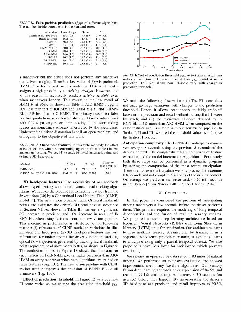
TABLE II: False positive prediction (fpp) of different algorithms.The number inside parenthesis is the standard error.

Algorithm Lane change Turns AllMorris et al. [50] SVM 15.3 (0.8) 13.3 (5.6) 24.0 (3.5)

Random-Forest 16.2 (3.3) 12.9 (3.7) 17.5 (4.0)HMM E 36.2 (6.6) 33.3 (0.0) 63.8 (9.4)HMM F 23.1 (2.1) 23.3 (3.1) 11.5 (0.1)

HMM E + F 30.0 (4.8) 21.2 (3.3) 40.7 (4.9)IOHMM 28.4 (1.5) 25.0 (0.1) 40.0 (1.5)

AIO-HMM 24.6 (1.5) 20.0 (2.0) 30.7 (3.4)S-RNN 16.2 (1.3) 16.7 (0.0) 19.2 (0.0)

F-RNN-UL 19.2 (2.4) 25.0 (2.4) 21.5 (2.1)F-RNN-EL 10.8 (0.7) 23.3 (1.5) 27.7 (3.8)

a maneuver but the driver does not perform any maneuver(i.e. drives straight). Therefore low value of fpp is preferred.HMM F performs best on this metric at 11% as it mostlyassigns a high probability to driving straight. However, dueto this reason, it incorrectly predicts driving straight evenwhen maneuvers happen. This results in the low recall ofHMM F at 36%, as shown in Table I. AIO-HMM’s fpp is10% less than that of IOHMM and HMM E+F , and F-RNN-EL is 3% less than AIO-HMM. The primary reason for falsepositive predictions is distracted driving. Drivers interactionswith fellow passengers or their looking at the surroundingscenes are sometimes wrongly interpreted by the algorithms.Understanding driver distraction is still an open problem, andorthogonal to the objective of this work.

TABLE III: 3D head-pose features. In this table we study the effectof better features with best performing algorithm from Table I in ‘Allmaneuvers’ setting. We use [4] to track 68 facial landmark points andestimate 3D head-pose.

Method Pr (%) Re (%) Time-to-maneuver (s)

F-RNN-EL 84.5 ± 1.0 77.1 ± 1.3 3.58F-RNN-EL w/ 3D head-pose 90.5 ± 1.0 87.4 ± 0.5 3.16

3D head-pose features. The modularity of our approachallows experimenting with more advanced head tracking algo-rithms. We replace the pipeline for extracting features from thedriver’s face [30] by a Constrained Local Neural Field (CLNF)model [4]. The new vision pipeline tracks 68 facial landmarkpoints and estimates the driver’s 3D head pose as describedin Section VI. As shown in Table III, we see a significant,6% increase in precision and 10% increase in recall of F-RNN-EL when using features from our new vision pipeline.This increase in performance is attributed to the followingreasons: (i) robustness of CLNF model to variations in illu-mination and head pose; (ii) 3D head-pose features are veryinformative for understanding the driver’s intention; and (iii)optical flow trajectories generated by tracking facial landmarkpoints represent head movements better, as shown in Figure 9.The confusion matrix in Figure 13 shows the precision foreach maneuver. F-RNN-EL gives a higher precision than AIO-HMM on every maneuver when both algorithms are trained onsame features (Fig. 13c). The new vision pipeline with CLNFtracker further improves the precision of F-RNN-EL on allmaneuvers (Fig. 13d).

Effect of prediction threshold. In Figure 12 we study howF1-score varies as we change the prediction threshold pth.

Fig. 12: Effect of prediction threshold pth. At test time an algorithmmakes a prediction only when it is at least pth confident in itsprediction. This plot shows how F1-score vary with change inprediction threshold.

We make the following observations: (i) The F1-score doesnot undergo large variations with changes to the predictionthreshold. Hence, it allows practitioners to fairly trade-offbetween the precision and recall without hurting the F1-scoreby much; and (ii) the maximum F1-score attained by F-RNN-EL is 4% more than AIO-HMM when compared on thesame features and 13% more with our new vision pipeline. InTables I, II and III, we used the threshold values which gavethe highest F1-score.Anticipation complexity. The F-RNN-EL anticipates maneu-vers every 0.8 seconds using the previous 5 seconds of thedriving context. The complexity mainly comprises of featureextraction and the model inference in Algorithm 1. Fortunatelyboth these steps can be performed as a dynamic programby storing the computation of the most recent anticipation.Therefore, for every anticipation we only process the incoming0.8 seconds and not complete 5 seconds of the driving context.On average we predict a maneuver under 0.20 millisecondsusing Theano [5] on Nvidia K40 GPU on Ubuntu 12.04.

IX. CONCLUSION

In this paper we considered the problem of anticipatingdriving maneuvers a few seconds before the driver performsthem. This problem requires the modeling of long temporaldependencies and the fusion of multiple sensory streams.We proposed a novel deep learning architecture based onRecurrent Neural Networks (RNNs) with Long Short-TermMemory (LSTM) units for anticipation. Our architecture learnsto fuse multiple sensory streams, and by training it in asequence-to-sequence prediction manner, it explicitly learnsto anticipate using only a partial temporal context. We alsoproposed a novel loss layer for anticipation which preventsover-fitting.

We release an open-source data set of 1180 miles of naturaldriving. We performed an extensive evaluation and showedimprovement over many baseline algorithms. Our sensoryfusion deep learning approach gives a precision of 84.5% andrecall of 77.1%, and anticipates maneuvers 3.5 seconds (onaverage) before they happen. By incorporating the driver’s3D head-pose our precision and recall improves to 90.5%

(a) IOHMM (b) AIO-HMM (c) F-RNN-EL (d) F-RNN-EL w/ 3D-pose

Fig. 13: Confusion matrix of different algorithms when jointly predicting all the maneuvers. Predictions made by algorithms are representedby rows and actual maneuvers are represented by columns. Numbers on the diagonal represent precision.

and 87.4% respectively. Potential application of our work isenabling advanced driver assistance systems (ADAS) to alertdrivers before they perform a dangerous maneuver, therebygiving drivers more time to react. We believe that our deeplearning architecture is widely applicable to many activityanticipation problems. Our code and data set are publiclyavailable on the project web-page.

Acknowledgement. We thank NVIDIA for the donationof K40 GPUs used in this research. We also thank SilvioSavarese for useful discussions. This work was supportedby National Robotics Initiative (NRI) award 1426452, Officeof Naval Research (ONR) award N00014-14-1-0156, andby Microsoft Faculty Fellowship and NSF Career Award toSaxena.

APPENDIX AMODELING MANEUVERS WITH AIO-HMM

Given T seconds long driving context C before the maneu-verM, we learn a generative model for the context P (C|M).The driving context C consists of the outside driving contextand the inside driving context. The outside and inside contextsare temporal sequences represented by the outside featuresxT1 = {x1, ..,xT } and the inside features zT1 = {z1, .., zT }respectively. The corresponding sequence of the driver’s latentstates is hT1 = {h1, .., hT }. x and z are vectors and h is adiscrete state.

P (C|M) =∑hT1

P (zT1 ,xT1 , h

T1 |M)

= P (xT1 |M)∑hT1

P (zT1 , hT1 |xT1 ,M)

∝∑hT1

P (zT1 , hT1 |xT1 ,M) (14)

We model the correlations between x, h and z with an AIO-HMM as shown in Figure 10. The AIO-HMM models thedistribution in equation (14). It does not assume any generativeprocess for the outside features P (xT1 |M). It instead modelsthem in a discriminative manner. The top (input) layer ofthe AIO-HMM consists of outside features xT1 . The outsidefeatures then affect the driver’s latent states hT1 , representedby the middle (hidden) layer, which then generates the insidefeatures zT1 at the bottom (output) layer. The events inside the

vehicle such as the driver’s head movements are temporallycorrelated because they are generally smooth. The AIO-HMMhandles these dependencies with autoregressive connections inthe output layer.Model Parameters. AIO-HMM has two types of parameters:(i) state transition parameters w; and (ii) observation emissionparameters (µ,Σ). We use set S to denote the possible latentstates of the driver. For each state h = i ∈ S, we parametrizetransition probabilities of leaving the state with log-linearfunctions, and parametrize the output layer feature emissionswith normal distributions.

Transition: P (ht = j|ht−1 = i,xt;wij) =ewij ·xt∑l∈S e

wil·xt

Emission: P (zt|ht = i,xt, zt−1;µit,Σi) = N (zt|µit,Σi)

The inside (vehicle) features represented by the output layerare jointly influenced by all three layers. These interactions aremodeled by the mean and variance of the normal distribution.We model the mean of the distribution using the outside andinside features from the vehicle as follows:

µit = (1 + ai · xt + bi · zt−1)µiIn the equation above, ai and bi are parameters that we learnfor every state i ∈ S. Therefore, the parameters we learn forstate i ∈ S are θi = {µi, ai, bi, Σi and wij |j ∈ S}, and theoverall model parameters are Θ = {θi|i ∈ S}.

A. Learning AIO-HMM parameters

The training data D = {(xTn1,n, z

Tn1,n)|n = 1, .., N} consists

of N instances of a maneuver M. The goal is to maximizethe data log-likelihood.

l(Θ;D) =N∑n=1

logP (zTn1,n|x

Tn1,n;Θ) (15)

Directly optimizing equation (15) is challenging because pa-rameters h representing the driver’s states are latent. Wetherefore use the iterative EM procedure to learn the model pa-rameters. In EM, instead of directly maximizing equation (15),we maximize its simpler lower bound. We estimate the lowerbound in the E-step and then maximize that estimate in theM-step. These two steps are repeated iteratively.E-step. In the E-step we get the lower bound of equation (15)by calculating the expected value of the complete data log-likelihood using the current estimate of the parameter Θ.

E-step: Q(Θ; Θ) = E[lc(Θ;Dc)|Θ,D] (16)

where lc(Θ;Dc) is the log-likelihood of the complete data Dcdefined as:

Dc = {(xTn1,n, z

Tn1,n, h

Tn1,n)|n = 1, .., N} (17)

lc(Θ;Dc) =N∑n=1

logP (zTn1,n, h

Tn1,n|x

Tn1,n;Θ) (18)

We should note that the occurrences of hidden variables hin lc(Θ;Dc) are marginalized in equation (16), and hence hneed not be known. We efficiently estimate Q(Θ; Θ) usingthe forward-backward algorithm [51].M-step. In the M-step we maximize the expected value of thecomplete data log-likelihood Q(Θ; Θ) and update the modelparameter as follows:

M-step: Θ = argmaxΘQ(Θ; Θ) (19)

Solving equation (19) requires us to optimize for the param-eters µ, a, b, Σ and w. We optimize all parameters expect wexactly by deriving their closed form update expressions. Weoptimize w using the gradient descent.

B. Inference of Maneuvers

Our learning algorithm trains separate AIO-HMM modelsfor each maneuver. The goal during inference is to determinewhich model best explains the past T seconds of the drivingcontext not seen during training. We evaluate the likelihood ofthe inside and outside feature sequences (zT1 and xT1 ) for eachmaneuver, and anticipate the probability PM of each maneuverM as follows:

PM = P (M|zT1 ,xT1 ) ∝ P (zT1 ,xT1 |M)P (M) (20)

Algorithm 2 shows the complete inference procedure. Theinference in equation (20) simply requires a forward-pass [51] of the AIO-HMM, the complexity of which isO(T (|S|2 + |S||z|3 + |S||x|)). However, in practice it is onlyO(T |S||z|3) because |z|3 � |S| and |z|3 � |x|. Here|S| is the number of discrete states representing the driver’sintention, while |z| and |x| are the dimensions of the insideand outside feature vectors respectively. In equation (20)P (M) is the prior probability of maneuver M. We assumean uninformative uniform prior over the maneuvers.

Algorithm 2 Anticipating maneuvers

input Driving videos, GPS, Maps and Vehicle Dynamicsoutput Probability of each maneuver

Initialize the face tracker with the driver’s facewhile driving do

Track the driver’s face [69]Extract features zT1 and xT1 (Sec. VI)Inference PM = P (M|zT1 ,xT1 ) (Eq. (20))Send the inferred probability of each maneuver to ADAS

end while

REFERENCES

[1] Bosch urban. http://bit.ly/1feM3JM. Accessed: 2015-04-23.

[2] 2012 motor vehicle crashes: overview. N. HighwayTraffic Safety Administration, Washington, D.C., Tech.Rep., 2013.

[3] A. Andreas, P. Lenz, and R. Urtasun. Are we ready forautonomous driving? the kitti vision benchmark suite. InProceedings of the IEEE Conference on Computer Visionand Pattern Recognition, 2012.

[4] T. Baltrusaitis, P. Robinson, and L-P. Morency. Con-strained local neural fields for robust facial landmarkdetection in the wild. In ICCV Workshop, 2013.

[5] F. Bastien, P. Lamblin, R. Pascanu, J. Bergstra, I. J.Goodfellow, A. Bergeron, N. Bouchard, and Y. Bengio.Theano: new features and speed improvements. DeepLearning and Unsupervised Feature Learning NIPS 2012Workshop, 2012.

[6] Y. Bengio and O. Delalleau. On the expressive powerof deep architectures. In Algorithmic Learning Theory,pages 18–36, 2011.

[7] Y. Bengio and O. Frasconi. An input output hmmarchitecture. Advances in Neural Information ProcessingSystems, 1995.

[8] M. Bennewitz, W. Burgard, G. Cielniak, and S. Thrun.Learning motion patterns of people for compliant robotmotion. International Journal of Robotics Research,2005.

[9] H. Berndt, J. Emmert, and K. Dietmayer. Continuousdriver intention recognition with hidden markov models.In IEEE Intelligent Transportation Systems Conference,2008.

[10] T. F. Cootes, G. J. Edwards, and C. J. Taylor. Active ap-pearance models. IEEE Transactions on Pattern Analysisand Machine Intelligence, 23(6), 2001.

[11] C. Cortes and V. Vapnik. Support-vector networks.Machine learning, 20(3), 1995.

[12] A. Criminisi, J. Shotton, and E. Konukoglu. Decisionforests for classification, regression, density estimation,manifold learning and semi-supervised learning. MSRTR, 5(6), 2011.

[13] Y. N. Dauphin, H. de Vries, J. Chung, and Y. Bengio.Rmsprop and equilibrated adaptive learning rates for non-convex optimization. arXiv:1502.04390, 2015.

[14] J. Donahue, L. A. Hendricks, S. Guadarrama,M. Rohrbach, S. Venugopalan, K. Saenko, andT. Darrell. Long-term recurrent convolutional networksfor visual recognition and description. In Proceedings ofthe IEEE Conference on Computer Vision and PatternRecognition, 2015.

[15] A. Doshi, B. Morris, and M. M. Trivedi. On-roadprediction of driver’s intent with multimodal sensorycues. IEEE Pervasive Computing, 2011.

[16] A. Dragan and S. Srinivasa. Formalizing assistive tele-operation. In Proceedings of Robotics: Science andSystems, 2012.

[17] A. Dragan and S. Srinivasa. Generating legible motion.In Proceedings of Robotics: Science and Systems, 2013.

[18] K. Driggs-Campbell, V. Shia, and R. Bajcsy. Improveddriver modeling for human-in-the-loop vehicular con-

trol. In Proceedings of the International Conference onRobotics and Automation, 2015.

[19] Y. Du, W. Wang, and L. Wang. Hierarchical recurrentneural network for skeleton based action recognition. InProceedings of the IEEE Conference on Computer Visionand Pattern Recognition, 2015.

[20] L. Fletcher, N. Apostoloff, L. Petersson, and A. Zelinsky.Vision in and out of vehicles. IEEE IS, 18(3), 2003.

[21] L. Fletcher, G. Loy, N. Barnes, and A. Zelinsky. Correlat-ing driver gaze with the road scene for driver assistancesystems. Robotics and Autonomous Systems, 52(1), 2005.

[22] B. Frohlich, M. Enzweiler, and U. Franke. Will this carchange the lane?turn signal recognition in the frequencydomain. In IEEE International Vehicle Symposium Pro-ceedings, 2014.

[23] A. Hannun, C. Case, J. Casper, B. Catanzaro, G. Diamos,E. Elsen, R. Prenger, S. Satheesh, S. Sengupta, andA. Coates. Deepspeech: Scaling up end-to-end speechrecognition. arXiv:1412.5567, 2014.

[24] S. El Hihi and Y. Bengio. Hierarchical recurrent neuralnetworks for long-term dependencies. In NIPS, 1995.

[25] S. Hochreiter and J. Schmidhuber. Long short-termmemory. Neural computation, 9(8), 1997.

[26] M. E. Jabon, J. N. Bailenson, E. Pontikakis,L. Takayama, and C. Nass. Facial expression analysisfor predicting unsafe driving behavior. IEEE PervasiveComputing, (4), 2010.

[27] A. Jain. Neuralmodels. https://github.com/asheshjain399/NeuralModels, 2015.

[28] A. Jain, S. Sharma, and A. Saxena. Beyond geometricpath planning: Learning context-driven user preferencesvia sub-optimal feedback. In Proceedings of the Inter-national Symposium on Robotics Research, 2013.

[29] A. Jain, D. Das, J. Gupta, and A. Saxena. Planit: Acrowdsourcing approach for learning to plan paths fromlarge scale preference feedback. In Proceedings of theInternational Conference on Robotics and Automation,2015.

[30] A. Jain, H. S. Koppula, B. Raghavan, S. Soh, andA. Saxena. Car that knows before you do: Anticipatingmaneuvers via learning temporal driving models. InICCV, 2015.

[31] A. Jain, S. Sharma, T. Joachims, and A. Saxena. Learningpreferences for manipulation tasks from online coactivefeedback. International Journal of Robotics Research,2015.

[32] Z. Kalal, K. Mikolajczyk, and J. Matas. Forward-backward error: Automatic detection of tracking failures.In Proceedings of the International Conference on Pat-tern Recognition, 2010.

[33] K. M. Kitani, B. D. Ziebart, J. A. Bagnell, and M. Hebert.Activity forecasting. In Proceedings of the EuropeanConference on Computer Vision. 2012.

[34] H. Koppula and A. Saxena. Anticipating human activitiesusing object affordances for reactive robotic response. InProceedings of Robotics: Science and Systems, 2013.

[35] H. Koppula and A. Saxena. Learning spatio-temporal

structure from rgb-d videos for human activity detectionand anticipation. In Proceedings of the InternationalConference on Machine Learning, 2013.

[36] H. Koppula and A. Saxena. Anticipating human activitiesusing object affordances for reactive robotic response.IEEE Transactions on Pattern Analysis and MachineIntelligence, 2015.

[37] H. Koppula, R. Gupta, and A. Saxena. Learning humanactivities and object affordances from rgb-d videos. In-ternational Journal of Robotics Research, 32(8), 2013.

[38] H. Koppula, A. Jain, and A. Saxena. Anticipatoryplanning for humanrobot teams. In ISER, 2014.

[39] M. Kuderer, H. Kretzschmar, C. Sprunk, and W. Burgard.Feature-based prediction of trajectories for socially com-pliant navigation. In Proceedings of Robotics: Scienceand Systems, 2012.

[40] N. Kuge, T. Yamamura, O. Shimoyama, and A. Liu. Adriver behavior recognition method based on a drivermodel framework. Technical report, SAE TechnicalPaper, 2000.

[41] P. Kumar, M. Perrollaz, S. Lefevre, and C. Laugier.Learning-based approach for online lane change intentionprediction. In IEEE International Vehicle SymposiumProceedings, 2013.

[42] J. Lafferty, A. McCallum, and F. Pereira. Conditionalrandom fields: Probabilistic models for segmenting andlabeling sequence data. In Proceedings of the Interna-tional Conference on Machine Learning, 2001.

[43] C. Laugier, I. E. Paromtchik, M. Perrollaz, MY. Yong,J-D. Yoder, C. Tay, K. Mekhnacha, and A. Negre. Prob-abilistic analysis of dynamic scenes and collision risksassessment to improve driving safety. ITS Magazine,IEEE, 3(4), 2011.

[44] M. Liebner, M. Baumann, F. Klanner, and C. Stiller.Driver intent inference at urban intersections using theintelligent driver model. In IEEE International VehicleSymposium Proceedings, 2012.

[45] B. Lucas and T. Kanade. An iterative image registra-tion technique with an application to stereo vision. InProceedings of the International Joint Conference onArtificial Intelligence, 1981.

[46] J. Mainprice and D. Berenson. Human-robot collabora-tive manipulation planning using early prediction of hu-man motion. In Proceedings of the IEEE/RSJ Conferenceon Intelligent Robots and Systems, 2013.

[47] I. Matthews and S. Baker. Active appearance modelsrevisited. International Journal of Computer Vision, 60(2), 2004.

[48] D. K. Misra, J. Sung, K. Lee, and A. Saxena. Tell medave: Context-sensitive grounding of natural languageto manipulation instructions. Proceedings of Robotics:Science and Systems, 2014.

[49] L. Morency, A. Quattoni, and T. Darrell. Latent-dynamicdiscriminative models for continuous gesture recognition.In Proceedings of the IEEE Conference on ComputerVision and Pattern Recognition, 2007.

[50] B. Morris, A. Doshi, and M. Trivedi. Lane change

intent prediction for driver assistance: On-road designand evaluation. In IEEE International Vehicle SymposiumProceedings, 2011.

[51] K. P. Murphy. Machine learning: a probabilistic per-spective. MIT press, 2012.

[52] J. Ngiam, A. Khosla, M. Kim, J. Nam, H. Lee, and A. Y.Ng. Multimodal deep learning. In Proceedings of theInternational Conference on Machine Learning, 2011.

[53] N. Oliver and A. P. Pentland. Graphical models for driverbehavior recognition in a smartcar. In IEEE InternationalVehicle Symposium Proceedings, 2000.

[54] R. Pascanu, T. Mikolov, and Y. Bengio. On the difficultyof training recurrent neural networks. arXiv:1211.5063,2012.

[55] M. Rezaei and R. Klette. Look at the driver, look atthe road: No distraction! no accident! In Proceedings ofthe IEEE Conference on Computer Vision and PatternRecognition, 2014.

[56] T. Rueda-Domingo, P. Lardelli-Claret, J. Luna delCastillo, J. Jimenez-Moleon, M. Garcia-Martin, andA. Bueno-Cavanillas. The influence of passengers onthe risk of the driver causing a car collision in spain:Analysis of collisions from 1990 to 1999. AccidentAnalysis & Prevention, 2004.

[57] M. S. Ryoo. Human activity prediction: Early recognitionof ongoing activities from streaming videos. In Proceed-ings of the International Conference on Computer Vision,2011.

[58] J. Shi and C. Tomasi. Good features to track. InProceedings of the IEEE Conference on Computer Visionand Pattern Recognition, 1994.

[59] V. Shia, Y. Gao, R. Vasudevan, K. D. Campbell, T. Lin,F. Borrelli, and R. Bajcsy. Semiautonomous vehicularcontrol using driver modeling. IEEE Transactions onIntelligent Transportation Systems, 15(6), 2014.

[60] E. A. Sisbot, L. F. Marin-Urias, R. Alami, and T. Simeon.A human aware mobile robot motion planner. IEEETransactions on Robotics, 2007.

[61] J. Sung, S. H. Jin, and A. Saxena. Robobarista: Ob-ject part-based transfer of manipulation trajectories fromcrowd-sourcing in 3d pointclouds. In Proceedings of theInternational Symposium on Robotics Research, 2015.

[62] I. Sutskever, O. Vinyals, and Q. V. Le. Sequence tosequence learning with neural networks. In Advances inNeural Information Processing Systems, 2014.

[63] A. Tawari, S. Sivaraman, M. Trivedi, T. Shannon, andM. Tippelhofer. Looking-in and looking-out vision forurban intelligent assistance: Estimation of driver attentivestate and dynamic surround for safe merging and braking.In IEEE IVS, 2014.

[64] S. Thrun, W. Burgard, and D. Fox. Probabilistic robotics.MIT press, 2005.

[65] M. E. Tipping. Sparse bayesian learning and the rel-evance vector machine. Journal of Machine LearningResearch, 1, 2001.

[66] C. Tomasi and T. Kanade. Detection and tracking of pointfeatures. International Journal of Computer Vision, 1991.

[67] M. Trivedi, T. Gandhi, and J. McCall. Looking-inand looking-out of a vehicle: Computer-vision-based en-hanced vehicle safety. IEEE Transactions on IntelligentTransportation Systems, 8(1), 2007.

[68] R. Vasudevan, V. Shia, Y. Gao, R. Cervera-Navarro,R. Bajcsy, and F. Borrelli. Safe semi-autonomous controlwith enhanced driver modeling. In American ControlConference, 2012.

[69] P. Viola and M. J. Jones. Robust real-time face detection.International Journal of Computer Vision, 57(2), 2004.

[70] H. Wang and C. Schmid. Action recognition withimproved trajectories. In Proceedings of the IEEEConference on Computer Vision and Pattern Recognition,2013.

[71] S. B. Wang, A. Quattoni, L. Morency, D. Demirdjian, andT. Darrell. Hidden conditional random fields for gesturerecognition. In Proceedings of the IEEE Conference onComputer Vision and Pattern Recognition, 2006.

[72] Y. Wang and Q. Ji. A dynamic conditional random fieldmodel for object segmentation in image sequences. InProceedings of the IEEE Conference on Computer Visionand Pattern Recognition, 2005.

[73] Z. Wang, K. Mulling, M. Deisenroth, H. Amor, D. Vogt,B. Scholkopf, and J. Peters. Probabilistic movementmodeling for intention inference in human-robot interac-tion. International Journal of Robotics Research, 2013.

[74] X. Xiong and F. De la Torre. Supervised descent methodand its applications to face alignment. In Proceedings ofthe IEEE Conference on Computer Vision and PatternRecognition, 2013.

[75] X. Xiong and F. De la Torre. Supervised descent methodfor solving nonlinear least squares problems in computervision. arXiv preprint arXiv:1405.0601, 2014.

[76] C. Zhang and Z. Zhang. A survey of recent advancesin face detection. Technical report, Microsoft Research,2010.

[77] B. D. Ziebart, N. Ratliff, G. Gallagher, C. Mertz, K. Pe-terson, J. A. Bagnell, M. Hebert, A. K. Dey, and S. Srini-vasa. Planning-based prediction for pedestrians. InProceedings of the IEEE/RSJ Conference on IntelligentRobots and Systems, 2009.