BRITISH STANDARD BS EN 689:1996BS 6069-3.7:1996

Workplace atmospheres — Guidance for the assessment of exposure by inhalation to chemical agents for comparison with limit values and measurement strategy

The European Standard EN 689:1995 has the status of a British Standard

BS EN 689:1996

This British Standard, having been prepared under the direction of the Health and Environment Sector Board, was published under the authority of the Standards Board and comes into effect on 15 April 1996

© BSI 03-1999

The following BSI references relate to the work on this standard:Committee reference EH/2Draft for comment 92/52696 DC

ISBN 0 580 25420 8

Committees responsible for this British Standard

The preparation of this British Standard was entrusted to Technical Committee EH/2, Air quality, upon which the following bodies were represented:

Association of Consulting ScientistsBritish Cement AssociationBritish Coal CoporationBritish Gas plcCombustion Engineering AssociationDepartment of HealthDepartment of the Environment (Her Majesty’s Inspectorate of Pollution)Department of Trade and Industry (Laboratory of the Government Chemist)Department of Trade and IndustryEngineering Equipment Users’ AssociationEuropean Resin Manufacturers’ AssociationGAMBICA (BEAMA Ltd.)Health and Safety ExecutiveInstitute of PetroleumInstitution of Environmental Health OfficersInstitution of Gas EngineersNational Society of Clean AirRoyal Society of Chemistry

The following bodies were also represented in the drafting of the standard, through sub-committees and panels:

Asbestos Information Centre Ltd.Asbestosis Research CouncilBritish Occupational Hygiene SocietyChemical Industries AssociationEngineering Equipment and Materials Users’ AssociationFibre Cement Manufacturers’ Association Ltd.Institute of EnergyInstitute of Occupational HygienistsInstitute of Occupational MedicineLondon Regional Transport

Amendments issued since publication

Amd. No. Date Comments

BS EN 689:1996

© BSI 03-1999 i

Contents

PageCommittees responsible Inside front coverNational foreword iiForeword 2Text of EN 689 3List of references Inside back cover

BS EN 689:1996

ii © BSI 03-1999

National foreword

This British Standard has been prepared by Technical Committee EH/2 and is the English language version of EN 689:1995 Workplace atmospheres — Guidance for the assessment of exposure by inhalation to chemical agents for comparison with limit values and measurement strategy, published by the European Committee for Standardization (CEN). The European Standard was prepared by Technical Committee 137, Assessment of workplace exposure, of CEN with the active participation and approval of the UK.BS 6069 is being published in a series of Parts and Sections that will generally correspond to particular European and International standards arising from the UK participation in the work of CEN/TC 137 and ISO/TC 146. This standard is being implemented as a Part in the BS 6069 series, and is one of several relating to workplace atmospheres that are being published as Sections of Part 3. Methods concerning stationary source emissions are being published as Sections of Part 4 of BS 6069. Topics related to other aspects of air quality characterization will be published as further Parts or Sections of BS 6069.The following Parts of BS 6069 have already been published:

— Part 1: Units of measurement;— Part 2: Glossary;— Part 3: Workplace atmospheres;— Part 4: Stationary source emissions.

Methods for the determination of specific constituents of ambient air are being published as Parts of BS 1747: Methods for measurement of air pollution.

A British Standard does not purport to include all the necessary provisions of a contract. Users of British Standards are responsible for their correct application.

Compliance with a British Standard does not of itself confer immunity from legal obligations.

Cross-references

Publication referred to Corresponding British Standard

EN 482:1994 BS EN 482:1994 Workplace atmospheres — General requirements for the performance of procedures for the measurement of chemical agents.

Summary of pagesThis document comprises a front cover, an inside front cover, pages i and ii, the EN title page, pages 2 to 28, an inside back cover and a back cover.This standard has been updated (see copyright date) and may have had amendments incorporated. This will be indicated in the amendment table on the inside front cover.

EUROPEAN STANDARD

NORME EUROPÉENNE

EUROPÄISCHE NORM

EN 689

February 1995

ICS 13.040.30

Descriptors: Air, quality, air pollution, workroom, exposure, contaminants, chemical compounds, estimation, maximum value, measurements, accident prevention

English version

Workplace atmospheres — Guidance for the assessment of exposure by inhalation to chemical agents for comparison

with limit values and measurement strategy

Atmosphères des lieux de travail — Conseils pour l’évaluation de l’exposition aux agents chimiques aux fins de comparaison avec des valeurs limites et stratégie de mesurage

Arbeitsplatzatmosphäre — Anleitung zur Ermittlung der inhalativen Exposition gegenüber chemischen Stoffen zum Vergleich mit Grenzwerten und Meßstrategie

This European Standard was approved by CEN on 1995-02-17. CEN membersare bound to comply with the CEN/CENELEC Internal Regulations whichstipulate the conditions for giving this European Standard the status of anational standard without any alteration.Up-to-date lists and bibliographical references cencerning such nationalstandards may be obtained on application to the Central Secretariat or to anyCEN member.This European Standard exists in three official versions (English, French,German). A version in any other language made by translation under theresponsibility of a CEN member into its own language and notified to theCentral Secretariat has the same status as the official versions.CEN members are the national standards bodies of Austria, Belgium,Denmark, Finland, France, Germany, Greece, Iceland, Ireland, Italy,Luxembourg, Netherlands, Norway, Portugal, Spain, Sweden, Switzerland andUnited Kingdom.

CEN

European Committee for StandardizationComité Européen de NormalisationEuropäisches Komitee für Normung

Central Secretariat: rue de Stassart 36, B-1050 Brussels

© 1995 All rights of reproduction and communication in any form and by any means reserved in allcountries to CEN and its members.

Ref. No. EN 689:1995 E

EN 689:1995

© BSI 03-19992

Foreword

This European Standard has been prepared by the Technical Committee CEN/TC 137 “Assessment of workplace exposure” the secretariat of which is held by DIN.This European Standard shall be given the status of a National Standard, either by publication of an identical text or by endorsement, at the latest by August 1995, and conflicting national standards shall be withdrawn at the latest by August 1995.According to the CEN/CENELEC Internal Regulations, the following countries are bound to implement this European Standard: Austria, Belgium, Denmark, Finland, France, Germany, Greece, Iceland, Ireland, Italy, Luxembourg, Netherlands, Norway, Portugal, Spain, Sweden, Switzerland, United Kingdom.

Contents

PageForeword 20 Introduction 31 Scope 32 Normative references 33 Definitions 34 General 45 Occupational exposure assessment 46 Periodic measurements 87 Report 98 Handling of data 9Annex A (informative) Minimum number of samples as a function of sampling duration 10Annex B (informative) Calculation of the occupational exposure concentration from individual analytical values 10Annex C (informative) Example of the application of a formal procedure for the evaluation of workers exposure based upon measurements within the occupational exposure assessment (OEA) 13Annex D (informative) Example of a possible approach to compare occupational exposure concentrations with limit values 16Annex E (informative) Establishing periodic measurements 18Annex F (informative) Example for the selection of intervals between periodic measurements 19Annex G (informative) Statistical analysis of data 20

PageAnnex H (informative) Bibliography 27Figure 1 — Schematic overview of procedure 5Figure C.1 — Example of a formal procedurefor the OEA 15Figure E.1 — Establishing periodic measurements 18Figure F.1 — Intervals between periodic measurements 20Figure G.1 — Moving weighted average chart 22Figure G.2 — Worked example of a probability plot 23Table A.1 — Minimum number of samples per shift in relation to sampling duration 10Table B.1 — Figures for example 3 11Table B.2 — Figures for example 4 12Table B.3 — Figures for example 5 12Table D.1 — Potential decisions 17Table G.1 — Plotting positions for normal probability paper 24Table G.2 — Plotting positions for normal probability paper 25Table G.3 — Example of ranking raw exposure data and determination of plotting positions 27

EN 689:1995

© BSI 03-1999 3

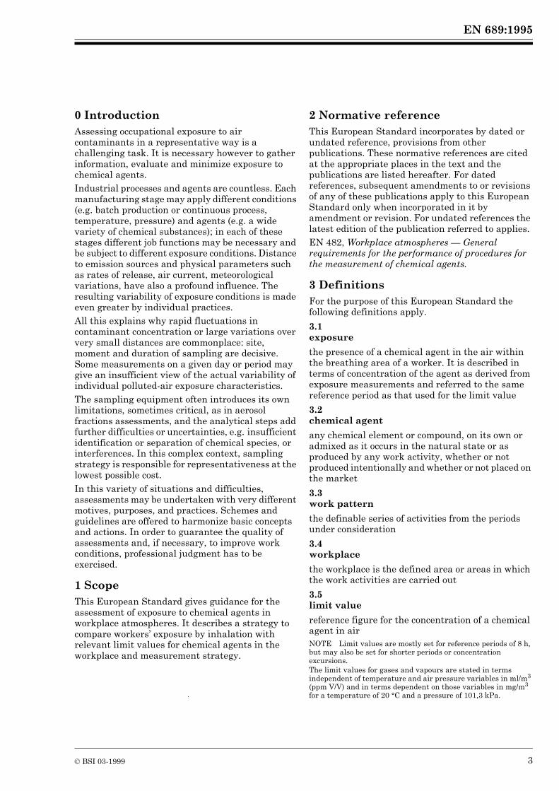
0 IntroductionAssessing occupational exposure to air contaminants in a representative way is a challenging task. It is necessary however to gather information, evaluate and minimize exposure to chemical agents.Industrial processes and agents are countless. Each manufacturing stage may apply different conditions (e.g. batch production or continuous process, temperature, pressure) and agents (e.g. a wide variety of chemical substances); in each of these stages different job functions may be necessary and be subject to different exposure conditions. Distance to emission sources and physical parameters such as rates of release, air current, meteorological variations, have also a profound influence. The resulting variability of exposure conditions is made even greater by individual practices.All this explains why rapid fluctuations in contaminant concentration or large variations over very small distances are commonplace: site, moment and duration of sampling are decisive. Some measurements on a given day or period may give an insufficient view of the actual variability of individual polluted-air exposure characteristics.The sampling equipment often introduces its own limitations, sometimes critical, as in aerosol fractions assessments, and the analytical steps add further difficulties or uncertainties, e.g. insufficient identification or separation of chemical species, or interferences. In this complex context, sampling strategy is responsible for representativeness at the lowest possible cost.In this variety of situations and difficulties, assessments may be undertaken with very different motives, purposes, and practices. Schemes and guidelines are offered to harmonize basic concepts and actions. In order to guarantee the quality of assessments and, if necessary, to improve work conditions, professional judgment has to be exercised.

1 ScopeThis European Standard gives guidance for the assessment of exposure to chemical agents in workplace atmospheres. It describes a strategy to compare workers’ exposure by inhalation with relevant limit values for chemical agents in the workplace and measurement strategy.

2 Normative referenceThis European Standard incorporates by dated or undated reference, provisions from other publications. These normative references are cited at the appropriate places in the text and the publications are listed hereafter. For dated references, subsequent amendments to or revisions of any of these publications apply to this European Standard only when incorporated in it by amendment or revision. For undated references the latest edition of the publication referred to applies.EN 482, Workplace atmospheres — General requirements for the performance of procedures for the measurement of chemical agents.

3 DefinitionsFor the purpose of this European Standard the following definitions apply.

3.1 exposure

the presence of a chemical agent in the air within the breathing area of a worker. It is described in terms of concentration of the agent as derived from exposure measurements and referred to the same reference period as that used for the limit value

3.2 chemical agent

any chemical element or compound, on its own or admixed as it occurs in the natural state or as produced by any work activity, whether or not produced intentionally and whether or not placed on the market

3.3 work pattern

the definable series of activities from the periods under consideration

3.4 workplace

the workplace is the defined area or areas in which the work activities are carried out

3.5 limit value

reference figure for the concentration of a chemical agent in airNOTE Limit values are mostly set for reference periods of 8 h, but may also be set for shorter periods or concentration excursions.The limit values for gases and vapours are stated in terms independent of temperature and air pressure variables in ml/m3 (ppm V/V) and in terms dependent on those variables in mg/m3 for a temperature of 20 °C and a pressure of 101,3 kPa.

EN 689:1995

4 © BSI 03-1999

The limit values for suspended matter are given in mg/m3 or multiples of that for actual environmental conditions (temperature, pressure) at the workplace. The limit values of fibres are given in fibres/m3 or fibres/cm3 for actual environmental conditions (temperature, pressure) at the workplace.

3.6 reference period

the specified period of time stated for the limit value of a specific agent. The reference period for a long term limit is normally 8 h and for short term limit normally 10 min to 15 min

3.7 personal sampler (or personal sampling device)

a device attached to a person that samples air in the breathing area

4 GeneralThe strategy includes two phases:

— an occupational exposure assessment (OEA): the exposure is compared with the limit value;— periodic measurements (PM) to regularly check if exposure conditions have changed.

The occupational exposure assessment is applied for the first evaluation and repeated after any significant change in working conditions, industrial process, products or chemicals or limit value. In this first phase no formal scheme of evaluation has to be followed, but it is left open to the professional judgment of the user to interpret and apply the guidelines. In the second phase, the frequency of the periodic measurements depends on the result of previous measurements.The requirement for future periodic measurements should have been established as a result of the initial OEA or subsequent amendments to it. These requirements include the scope and frequency of measurements to be made. The periodic measurements follow a procedure which is defined in the occupational exposure assessment. In certain cases the periodic measurements can be omitted.Figure 1 gives a schematic overview of the procedures described in this European Standard.

5 Occupational exposure assessment5.1 Assessment strategy

5.1.1 General

The workpattern and workplace under consideration have to be described within the occupational exposure assessment.

The occupational exposure assessment comprises three steps:

— identification of potential exposure (list of substances);— determination of workplace factors;— assessment of exposures.

5.1.2 Identification of potential exposure

The preparation of a list of all chemical agents in the workplace concerned is an essential first step to the identification of the potential for hazardous exposure. The list includes, as far as any of them can contribute to exposures, primary products, impurities, intermediates, final products, reaction products and byproducts.Appropriate limit values have to be obtained and where these are not available other criteria may be used for the purpose.In the case of a process not yet in operation this identification may be partially carried out by using relevant available data but such identification will need to be confirmed at a later stage.

5.1.3 Determination of workplace factors

In this step the work processes and procedures are evaluated to gauge the potential for exposure to chemical agents by a detailed review of, for example:

— job functions: i.e. tasks;— work patterns and techniques;— production processes;— workplace configuration;— safety precautions and procedures;— ventilation installations and other forms of engineering control;— emission sources;— exposure times;— workload.

5.1.4 Assessment of exposure

An assessment of exposures which brings together the identification of potential exposures, the workplace factors and the links between them, requires a structured approach and may be conducted in three stages:

— an initial appraisal;— a basic survey;— a detailed survey.

For the comparison with the limit value the data about temporal and spatial distribution of the concentrations of the substances in the workplace air have to be collected.

EN 689:1995

© BSI 03-1999 5

Figure 1 — Schematic overview of procedure

EN 689:1995

6 © BSI 03-1999

However, it is not necessary to use every stage of the assessment. If it is expected that exposure exceeds the limit value or if it is clearly determined that exposure is well below the limit value, then the occupational exposure assessment can be concluded and action taken in accordance with 5.5.

5.1.4.1 Initial appraisal

The initial appraisal, by referring to the list of chemical agents (see 5.1.2) and the workplace factors (see 5.1.3) yields a consideration of the likelihood of exposure.The variables affecting the airborne concentrations of substances close to an individual are:

— the number of sources from which agents are released;— the production rate in relation to production capacity;— the rate of release from each source;— the type and position of each source;— the dispersal of the agents by air movement;— the type and effectiveness of exhaust and ventilation systems.

The variables related to the individual’s actions and behaviour are:

— how close the individual is to the sources;— length of time spent in an area;— the individual’s own work practices.

If this initial appraisal shows that the presence of an agent in the air at the workplace cannot for certain be ruled out this agent needs further consideration (see 5.1.4.2 and 5.1.4.3).

5.1.4.2 Basic survey

The basic survey provides quantitative information about exposure of workers concerned, taking particular account of tasks with high exposures. Possible sources of information are:

— earlier measurements;— measurements from comparable installations or workprocesses;— reliable calculations based upon relevant quantitative data.

If the information obtained is insufficient to enable valid comparison to be made with the limit values, it has to be supplemented by workplace measurements.

5.1.4.3 Detailed survey

The detailed survey is aimed at providing validated and reliable information on exposure when this is close to the limit value.

5.2 Measurement strategy

Generally, for the purposes of obtaining quantitative data on exposures by measurement, an approach should be taken which enables the most efficient use of resources.Where it is suspected that exposure levels are well below or above the limit values, these clear cases may be confirmed by the use of techniques which are easily applied and which may be less accurate. Other possibilities may be worst case measurements, sampling near emission source or screening measurements (see 4.2 to 4.4 of EN 482:1994). Thus, in these cases, the occupational exposure assessment may often be completed without further investigation.In other cases, where exposures are suspected to be close to the limit values, then it will be necessary to undertake a more accurate investigation, making full use of the capabilities of instrumental and analytical techniques, where appropriate (see 4.5 of EN 482:1994).

5.2.1 Selection of workers for exposure measurements

It is not possible to be precise as to the procedure for selection of a worker or group of workers for exposure measurements. However, some general guidelines can be given.One possible approach is to sample workers randomly from within the whole exposed population. However, from a statistical standpoint this requires a relatively large number of samples. In many workplaces if this approach is used there is a considerable risk that small subgroups of highly exposed personnel will be missed.The preferred approach is to subdivide the exposed population into homogeneous groups with respect to exposure. The variability of exposure levels is smaller for well-defined groups than for the exposed workforce as a whole. Thus, where a group of workers is performing identical or similar tasks at the same place and has a similar exposure, sampling such as representative of the group may be carried out within that group.Groupings have the practical advantage that resources can be concentrated on those groups of workers with the highest exposure.It is necessary to verify that groups have been properly selected by critical study of the work patterns and examination of the preliminary sampling data.

EN 689:1995

© BSI 03-1999 7

Within a homogeneous group exposure patterns will still be subject to both random and systematic variations. Professional judgment as to the homogeneity of the defined groups is essential. However, as a rule of thumb, if an individual exposure is less than half or greater than twice the arithmetic mean, the relevant work factors should be closely re-examined to determine whether the assumption of homogeneity was correct.Professional judgment is also required when deciding on sample size, particularly when small groups are concerned. However, as a general rule, sampling should be carried out for at least one employee in ten in a properly selected homogeneous group.The frequency at which trials should be made and the number of group members selected for measurements will depend on how accurate the estimates of the distribution parameters such as the mean and variance need to be, on how far exposures are below the limit value, and the significance of the prevailing exposure levels and the properties of the substances. Where the arithmetic mean of exposure measurements is close to half of the limit value it is likely that some results will exceed the limit value.If exposure is characterized by peak exposures, then these peaks have to be assessed according to the short term limit requirements, if any.

5.2.2 Fixed-point measurements

Fixed-point measuring systems may be used if the results make it possible to assess exposure of the worker at the workplace.Samples should as far as possible be taken at breathing height and in the immediate vicinity of workers. If in doubt the point of greatest risk is to be taken as the measuring point.

5.2.3 Selection of measurement conditions

5.2.3.1 Representative measurements

Taking into account the possible influences of all relevant workplace factors, measurement conditions have to be selected in such a way that the measurement results give a representative view of exposure under working conditions.The best estimate of an individual’s exposure is obtained by taking breathing zone samples for the entire working period. Full information on the variation of exposures may be obtained with direct reading instruments or by providing fresh samples as work activities change. This optimum is not always practical and the distribution of actual sampling time should be arranged so that it mostly covers those activities about which there is least information about the likely exposures.

Measurements should be performed on sufficient days and during various specific operations in order to gain insight into the pattern of exposure. It is important to consider different episodes during which exposure conditions may vary (night and day cycles, seasonal variations).

5.2.3.2 Worst-case measurements

When it is possible to identify clearly episodes where higher exposures occur, e.g. a high emission due to certain working activities, sampling periods can be selected containing these episodes. This approach is called worst case sampling.Worst case conditions may be discovered by screening measurements which can show the variations of concentrations in time and space (see 4.2 of EN 482:1994).If, for the purposes of determining the 8 h time-weighted average exposure, the concentrations found in these cases are presumed to apply for the whole of the working period, then this presumption will err on the side of safety.Thus, sampling efforts can be concentrated on periods with relatively unfavourable conditions.

5.2.4 Measurement pattern

The pattern of sampling can be influenced by a number of practical issues, such as the frequency and duration of particular tasks and the optimal use of occupational hygiene and analytical resources. Within these constraints the pattern needs to be arranged so that the data are representative of identified tasks for known periods. This is particularly important for the many workplaces where the work is varied throughout the work period which itself may be interrupted and not approximating to an 8 h total period per day.Provided that the concentration patterns during a working period do not change significantly, sampling times may be chosen which do not cover the entire period. The duration of an individual sample is often dictated by constraints of the method of sampling and analysis in practice.However, unsampled time remains a serious weakness in the credibility of any exposure measurement. During this time careful observation of events is necessary. The assumption that changes have not occurred in the unsampled period have to be always critically examined.In cases where sampling duration is shorter than the whole period of exposure during a shift the minimum number of samples may vary. Annex A contains a table which can be used as a guide in the case of a homogeneous working period.

EN 689:1995

8 © BSI 03-1999

If exposure is characterized by peak exposures, then these peaks have to be assessed according to the short-term limit requirements, if any.

5.3 Measurement procedure

The measurement procedure needs to give results representative of worker exposure. To measure the exposure of the worker at the workplace, personal sampling devices should be used when possible, attached to workers’ bodies.The measurement procedure should contain:

— the agents;— the sampling procedure;— the analytical procedure;— the sampling location(s);— the duration of sampling;— the timing and the interval between measurements;— the calculations which yield the occupational exposure concentration from the individual analytical values (see Annex B);— further technical instructions concerning the measurements; — the jobs to be monitored.

5.4 Exposure to mixtures

If workers are exposed simultaneously or consecutively to more than one agent, this fact needs to be taken into consideration.

5.5 Conclusion of the occupational exposure assessment

The occupational exposure concentration is the arithmetic mean of the measurements in the same shift with respect to the appropriate reference period of the limit value of the agent under consideration. In the case of varying averaging times this has to be accounted for by time-weighting the values. Examples are presented in Annex B.A number of schemes can be devised to compare exposures with the limit values. Examples are given in Annex C and Annex D. However, whatever scheme is used, one of the three following conclusions should be made.

a) The exposure is above the limit value. Then:— the reasons for the limit value being exceeded should be identified and appropriate measures to remedy the situation should be implemented as soon as possible;— the occupational exposure assessment should be repeated when appropriate measures have been implemented.

b) The exposure is well below the limit value and is likely to remain so on a long-term basis due to the stability of conditions at the workplace and the arrangement of the work process. In this case periodic measurements are not needed. In such cases a regular check is required on whether the occupational exposure assessment leading to that conclusion is still applicable.c) The exposures do not fit into categories a) or b). Here, even though exposure may be below the limit value, periodic measurements are still required.

In certain cases the periodic measurements can be omitted, depending on the properties of the agent and the work process. Criteria for deciding on whether or not to carry out periodic measurements are laid down in the technical guidelines issued by the responsible authorities. An example of a procedure for considering if and when periodic measurements are required is given in Annex E.If periodic measurements are necessary the measurement procedure to be used has to be defined. The purpose of the periodic measurements is to check the validity of the occupational exposure assessment and to recognize changes of exposure with time. The elements to be contained in the measurement procedure are given in 5.3.The occupational exposure assessment is only concluded when a report has been made of the work done. This report needs to contain the details mentioned in clause 7.

6 Periodic measurementsThe emphasis of periodic measurements is on longer term objectives such as checking that control measures remain effective. Information is likely to be obtained on trends or changes in pattern of exposure so that action can be taken before excessive exposures occur.As periodic monitoring is designed to provide a rather different type of information from that obtained during the OEA, it follows the sampling strategies used may not be the same.Different types of strategy are available in relation to the particular circumstances of the workplace and the reliability of the information required. One particular strategy shall be selected and be kept over the time.For the results of a periodic sampling programme to be of real use it is essential to be able to compare consecutive sets of results. This implies that the how, where and when of collecting samples needs to be rigorously planned to ensure that the overall error can be estimated and that genuine change in the exposure pattern can be recognized.

EN 689:1995

© BSI 03-1999 9

Periodic monitoring programmes that are not well designed can produce an apparently reassuring bulk of paperwork but the real information content may be low and interpretation with any degree of confidence extremely difficult.Where enough data have been obtained for statistical analysis there are several possible methods of using the relevant limit value to evaluate the information.When data are shown to fit theoretical distributions considerable care however has be taken not to dismiss outlying results even though the bulk of the data has proved a good fit. Many sets of data are of limited size and only a few results are scattered towards the high tail end. In addition the high results may be due to non-random effects arising from non-homogeneous groupings of workers. If a small sub-group has consistently higher exposures this real effect can not be dismissed as a random variation as a potential risk to health may be missed, see Annex G.The interval between measurements should be established after consideration of the following factors:

— process cycles, including when normal working conditions occur;— consequences of control failure;— closeness to the limit value;— effectiveness of process controls;— time required to re-establish control;— the temporal variability of the results.

Such a consideration of all these factors may lead to intervals between periodic measurements varying, for example, from less than a week to more than a year.Annex E gives an example of procedure for determining when and if periodic measurements are required.Another example of a periodic measurements scheme is given in Annex F.If an occupational exposure concentration exceeds the limit value, the reason for the limit value being exceeded has to be identified and, when appropriate, measures to remedy the situation have to be implemented as soon as possible and the occupational exposure assessment has to be validated.

7 ReportReports shall be written of the occupational exposure assessment and of any periodic measurement. Each report should give reasons for the procedures adopted in the particular workplace.The report has to contain:

— the name of the person(s) or institutions undertaking the assessment and the measurements;— the name of the substances considered;— name and address of company;— the description of the workplace factors including the working conditions during the measurements;— the purpose of the measurement procedure;— the measuring procedure;— the time schedule (date, beginning and end of sampling);— the occupational exposure concentrations;— all events or factors liable to influence appreciably the results;— details of quality assurance if any;— result of the comparison with the limit value.

The airborne concentration of chemical agents is normally the mass of the substance in the unit of air volume.The concentration for gases and vapours is expressed in terms independent of temperature and air pressure variables in ml/m3 (ppm) and in terms dependent of those variables in mg/m3 for a temperature of 20 °C and a pressure of 101,3 kPa.The concentration for suspended matter is given in mg/m3 for actual environmental conditions in the workplace.The concentration of asbestos fibres is given in fibres/m3.The concentration of other fibres may be expressed in units similar to those for suspended matter or asbestos fibres or both depending upon the units used in the standards applied.

8 Handling of dataAnnex D and Annex G give examples of statistical analysis of data obtained during the occupational exposure assessment and periodic measurements.

EN 689:1995

10 © BSI 03-1999

Annex A (informative) Minimum number of samples as a function of sampling durationThe minimum number of samples required for a homogeneous working period may be established by statistical analysis but as a guide Table A.1 may be used.

Table A.1 — Minimum number of samples per shift in relation to sampling

duration

Table A.1 gives a guide for sampling in work processes with homogeneous exposure patterns. It is a combination of practical experience and statistical arguments, as generally statistics in occupational exposure assessments can only be used as a guideline for the findings of a professional. The reason for this is, that variations of workplace concentrations originate from techniques, work patterns and processes. Besides this, work processes normally take place in closed workshops, so that emissions into the workplace atmosphere sometimes have a long time lag (Markov type processes). Nevertheless, if the sampling duration time of an individual sample decreases considerably in relation to the total exposure duration, then statistical arguments can be used to decrease the minimum number of samples per shift.The timetable is based on the assumption that approximately 25 % of the exposure duration is sampled, provided that the working period does not involve significant changes in exposure.With very short sampling duration times this would involve an enormous number of single samples, e.g. 720 for a 10 s sampling duration time. For practical reasons this amount is not feasible. Sufficient statistical stability is certainly reached with 30 samples per shift. This means also that variations of the shift length do not affect this minimum number. The number of samples can only be decreased in cases of considerably shorter times of exposure.The Table A.1 gives a crude interpolation between these two extremes. It gives minimum numbers for a selection of sampling duration times, which often can occur in workplace analysis: 10 s relates to grab sampling techniques, 1 min to 5 min to detector tubes. A sampling duration time of 15 min to 60 min can be used for sampling on charcoal or silica (e.g. NIOSH type tubes), and at least 1 h for dust sampling on filters.

Annex B (informative) Calculation of the occupational exposure concentration from individual analytical valuesThis procedure only applies when the limit value has been set as an 8 h time weighted average.The term “8 h reference period” relates to the procedure whereby the occupational exposures in any shift period are treated as equivalent to a single uniform exposure for 8 h (the 8 h time-weighted average (TWA) exposure).The 8 h TWA may be represented mathematically by:

Sampling duration time Minimum number of samples per shift

10 s1 min5 min15 min30 min1 h$ 2 h

302012

4321

EN 689:1995

© BSI 03-1999 11

where

The following examples are given only to illustrate how time weighted averages are to be calculated.Example 1The operator works for 7 h 20 min on a process in which he is exposed to a substance with a limit value. The average exposure concentration during that period is measured as 0,12 mg/m3.The 8 h TWA therefore is:

7 h 20 min (7,33 h) at 0,12 mg/m3 40 min (0, 67 h) at 0 mg/m3

; that is = 0,11 mg/m3.

Example 2The operator works for 8 h on a process in which he is exposed to a substance with a limit value. The average exposure concentration during that period is measured as 0,15 mg/m3.The 8 h TWA therefore is:

= 0,15 mg/m3

Example 3Working periods may be split into several sessions for the purposes of sampling to take account of rest and meal breaks, etc. This is illustrated by the following example:

Table B.1 — Figures for example 3

Exposure was found to be zero during the periods 10.30 to 10.45, 12.45 to 13.30 and 15.30 to 15.45.The 8 h TWA therefore is:

= 0,19 mg/m3

Example 4An operator works for 8 h during the night shift on a process in which he is intermittently exposed to a substance with a limit value. The operator’s work pattern during the working period should be known and the best available data relating to each period of exposure should be applied in calculating the 8 h TWA. These should be based on direct measurement, estimates based on data already available or reasonable assumptions.

ci is the occupational exposure concentration;ti is the associated exposure time in hours;

is the shift length in hours.

Working period Exposuremg/m3

Duration of samplingh

08.00 to 10.30 0,32 2,5

10.45 to 12.45 0,07 2

13.30 to 15.30 0,20 2

15.45 to 17.15 0,10 1,5

0,12 7,33× 0 0,67×+8

---------------------------------------------------------

0,15 8×8

----------------------

0,32 2,5 0,07 2 0,2 2 0,1 1,5 0 1,25×+×+×+×+×8

-------------------------------------------------------------------------------------------------------------------------------------------------

0,8 0,14 0,4 0,15 0+ + + +8

---------------------------------------------------------------------=

EN 689:1995

12 © BSI 03-1999

Table B.2 — Figures for example 4

Exposure was found to be zero during the office work and working in the canteen.The 8 h TWA is:

Example 5A worker is engaged in a dusty process at a factory which is running at maximum production. He agrees to work his machine an additional three hours on one day to complete some orders.

Table B.3 — Figures for example 5

Total time at work (“shift length”) = 11,5 hThe 8 h TWA is:

= 5,2 mg/m3

Assume that the breaks were taken well away from the work areas and that personal sampling produced the non-zero results. In this example the additional 3 h work has significantly increased the 8 h TWA which would, without the additional exposure have been:

= 3,0 m g/m3

Working period Task Exposuremg/m3

Timeh

22.00 to 24.00 Helping in workshop 0,10 (derived from exposure of group working fulltime in workshop)

2

24.00 to 01.00 Office work 0 1

01.00 to 04.00 Working in canteen 0 3

04.00 to 06.00 Cleaning-up after breakdown in workshop

0,21 (measured) 2

Working period Task Exposuremg/m3

Timeh

07.30 to 08.15 Setting up zero 0,75

08.15 to 10.30 Product run 1 5,3 2,25

10.30 to 11.00 Break zero 0,50

11.00 to 13.00 Product run 2 4,7 2,00

13.00 to 14.00 Lunch zero 1,00

14.00 to 15.45 General tidying 1,6 1,75

15.45 to 16.00 Break zero 0,25

16.00 to 19.00 Extra product run 5,7 3,00

0,10 2 0,21 2 0 4×+×+×8

------------------------------------------------------------------------ 0,078 mg m3⁄=

0 0,75× 5,3 2,25 0+ 0,50× 4,7 2,00 0 1,00 1,6 1,75 0 0,25 5,7 3,00×+×+×+×+×+×+8

---------------------------------------------------------------------------------------------------------------------------------------------------------------------------------------------------------------------------------------------

41,2258

------------------=

5,3 2,25 4,7 2,00 1,6 1,75×+×+×8

--------------------------------------------------------------------------------------------

EN 689:1995

© BSI 03-1999 13

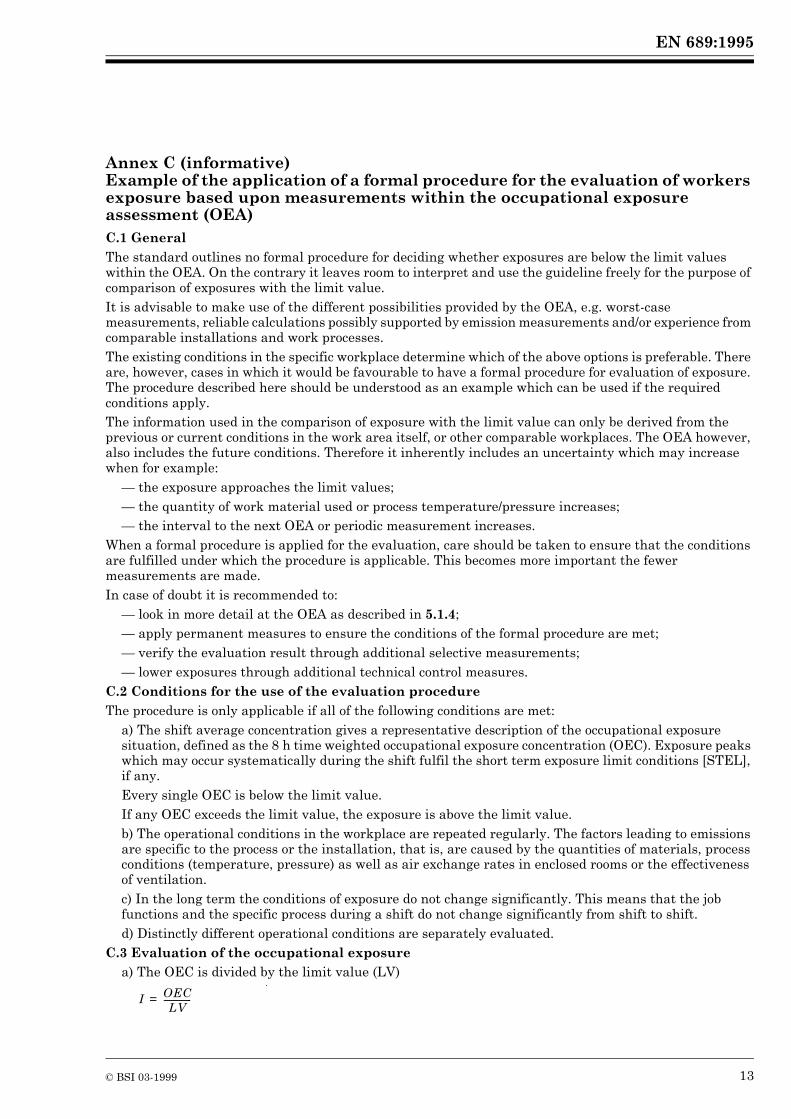
Annex C (informative) Example of the application of a formal procedure for the evaluation of workers exposure based upon measurements within the occupational exposure assessment (OEA)C.1 GeneralThe standard outlines no formal procedure for deciding whether exposures are below the limit values within the OEA. On the contrary it leaves room to interpret and use the guideline freely for the purpose of comparison of exposures with the limit value.It is advisable to make use of the different possibilities provided by the OEA, e.g. worst-case measurements, reliable calculations possibly supported by emission measurements and/or experience from comparable installations and work processes.The existing conditions in the specific workplace determine which of the above options is preferable. There are, however, cases in which it would be favourable to have a formal procedure for evaluation of exposure. The procedure described here should be understood as an example which can be used if the required conditions apply.The information used in the comparison of exposure with the limit value can only be derived from the previous or current conditions in the work area itself, or other comparable workplaces. The OEA however, also includes the future conditions. Therefore it inherently includes an uncertainty which may increase when for example:

— the exposure approaches the limit values;— the quantity of work material used or process temperature/pressure increases;— the interval to the next OEA or periodic measurement increases.

When a formal procedure is applied for the evaluation, care should be taken to ensure that the conditions are fulfilled under which the procedure is applicable. This becomes more important the fewer measurements are made.In case of doubt it is recommended to:

— look in more detail at the OEA as described in 5.1.4;— apply permanent measures to ensure the conditions of the formal procedure are met;— verify the evaluation result through additional selective measurements;— lower exposures through additional technical control measures.

C.2 Conditions for the use of the evaluation procedureThe procedure is only applicable if all of the following conditions are met:

a) The shift average concentration gives a representative description of the occupational exposure situation, defined as the 8 h time weighted occupational exposure concentration (OEC). Exposure peaks which may occur systematically during the shift fulfil the short term exposure limit conditions [STEL], if any.Every single OEC is below the limit value.If any OEC exceeds the limit value, the exposure is above the limit value.b) The operational conditions in the workplace are repeated regularly. The factors leading to emissions are specific to the process or the installation, that is, are caused by the quantities of materials, process conditions (temperature, pressure) as well as air exchange rates in enclosed rooms or the effectiveness of ventilation.c) In the long term the conditions of exposure do not change significantly. This means that the job functions and the specific process during a shift do not change significantly from shift to shift.d) Distinctly different operational conditions are separately evaluated.

C.3 Evaluation of the occupational exposurea) The OEC is divided by the limit value (LV)

I OECLV

--------------=

EN 689:1995

14 © BSI 03-1999

For results below the limit of detection, half of the detection limit should be used. “I” is called the substance index.b) If the index for the first shift is I k 0,1, exposure is below the limit value. If furthermore, it can be shown that this value is representative for the long term workplace conditions the periodic measurements can be omitted.c) If each single index of at least three different shifts is I k 0,25, exposure is below the limit value. If furthermore it can be shown that these values are representative for the long term workplace conditions the periodic measurements can be omitted.d) If the indices of at least three different shifts are all I k 1, and the geometric mean of all measurements is k 0,5, then exposure is below the limit value.e) If an index is I > 1, exposure is above the limit value.f) In all cases that do not fit into a) to e) the procedure leads to no decision.

If any of the conditions of b), c) or d) apply, then the occupational exposure assessment can be terminated.In the cases c) or d) the OEC can be interpreted as the first periodic measurement. Its result then may determine the time interval for the next periodic measurement.If workers are exposed simultaneously or consecutively to more than one agent, this fact needs to be taken into consideration.Figure C.1 gives a scheme for this formal evaluation procedure.

EN 689:1995

© BSI 03-1999 15

Figure C.1 — Example of a formal procedure for the OEA

EN 689:1995

16 © BSI 03-1999

Annex D (informative) Example of a possible approach to compare occupational exposure concentrations with limit valuesD.1 IntroductionThe scheme of comparison of OEC with limit values presented here is based on statistical principles. Specialized literature in this field can be consulted for further details (see the references in Annex H).This approach has been particularly adapted for the assessment of repetitive or steady state situations of occupational exposure to chemical agents. Such situations occur frequently in plants where tasks at the workplace are well defined and planned.Refineries and large plants of chemical production represent typical industrial activities for which this scheme is well adapted.After measurements are performed, comparison with the limit value is based on the widely used model of a log-normal distribution of concentrations (after checking its applicability) and applies basic statistics to determine the probability of exceeding the limit value.D.2 Workplace measurementsThe workplace measurements include the following steps:

a) Selection of an homogeneous exposure group (H.E.G.) of workers. The H.E.G. is defined as a group of workers with similar work patterns, but not necessarily at the same time. These workers represent basically similar exposure conditions.b) Achievement of a minimum of six measurements within the H.E.G. in the breathing zone of individuals; the sampling programme should aim to be representative of the H.E.G.c) Identification and calibration of a distribution model fitting the experimental results.The lognormal model is the most frequently proposed statistical model [1]. A cumulative probability plot [2] is recommended at this step of the initial analysis (see Annex G). Such a plot provides the possibility to check the homogeneity of the exposure data set.Several test statistics, as those of Shapiro Wilk [3] or Filliben Fit Factor [4], for example, are available to check the statistical hypothesis of lognormal distribution.d) Once the distribution model has been adjusted, calculation of the probability of exceeding the limit value, with its confidence interval.

D.3 Conclusion of the occupational exposure assessmentDepending on the probability of exceeding the limit value, three possibilities can result:

The exposure is well below the limit value; other measurements are not necessary unless any significant change occurs in working conditions. In the latter case, a new occupational exposure assessment is necessary.

The exposure seems to be below the limit value, but it has to be confirmed by periodic measurements.Periodic measurements should be planned only in this orange situation (see clause D.4).

The probability of exceeding the limit value is too high; appropriate actions have to be taken as soon as possible to reduce exposure. After these actions are completed, a new occupational exposure assessment should be conducted.These threshold values of probability are only provided for guidance. A certain latitude of decision should be allowed, especially if the probability has a wide confidence interval.In this case, a typical approach could consist of:

— a critical examination of the effective homogeneity of the H.E.G. (quality of the lognormal fit and value of the geometric standard deviation, typically less than 3);— critical examination of the technical quality of the measurements;

Probability k 0,1 % Green situation

0,1 % < probability k 5 % Orange situation

5 % < probability Red situation

EN 689:1995

© BSI 03-1999 17

— a plan of the complementary personal sampling within the H.E.G. before any conclusion.D.4 Periodic measurementsD.4.1 GeneralIn this example, periodic measurements are a modifiable schedule of personal sampling measurements within the H.E.G. The sampling frequency depends on the results of the previous measurements:

— it increases if the exposure approaches the limit value;— it decreases if it is well below the limit value.

D.4.2 Initial frequency of samplingA time unit (always less than or equal to one week) is determined depending on several factors, including:

— the working routine of the unit;— the type of limit value (short term exposure limit or 8 h time weighted average);— the response time of the analytical laboratory.

The initial periodicity equals 8 time units (basic schedule).D.4.3 Modifications to the scheduleThe basic schedule is modified according to the results of previous measurements.Each measurement is compared to four reference levels (LV: Limit Value):N1 = 0,40 LVN2 = 0,70 LVN3 = 1,00 LVN4 = 1,50 LVPotential decisions are summarized in Table D.1.

Table D.1 — Potential decisions

Situation Result of measurements Decision

1 CkN1 twice consecutively The three following scheduled measurements are not carried out

2 C kN2 The basic schedule is continued

3 N2 < C k N4 One additional measurement during the time unit

4 N2 < C k N4 for two consecutive time units

An additional measurement is carried out in each of the four subsequent programmed intervals. If this interval is one unit of time, immediate action to reduce exposure.

5 N3 < C k N4 twice consecutively Immediate action to reduce exposure

6 C > N4 Immediate action to reduce exposureIn situations 3 and 4, if C > N3, the reasons for the limit value being exceeded need to be identified and appropriate measures to remedy the situation need to be implemented as soon as possible.

EN 689:1995

18 © BSI 03-1999

Annex E (informative) Establishing periodic measurements

Figure E.1 — Establishing periodic measurements

EN 689:1995

© BSI 03-1999 19

Annex F (informative) Example for the selection of intervals between periodic measurementsIf the occupational exposure assessment shows that exposure is below the limit value (see 5.5), subsequent measurements at appropriate intervals should, if necessary, be taken to ensure that the situation continues to prevail.The nearer the concentration recorded comes to the limit value, the more frequently measurements should be taken.Periodic measurements are carried out with the measurement procedure defined at the end of the occupational exposure assessment (see 5.5).An example for the selection of intervals between periodic measurements which has proved useful in practice is the following one (see Figure F.1).The first measurement is carried out within an interval of 16 weeks after the occupational exposure assessment has shown that periodic measurements are needed.The maximum time interval to the next periodic measurement depends on the result of the previous measurement.This interval is:

— 64 weeks if the occupational exposure concentration does not exceed 1/4 limit value;— 32 weeks if the occupational exposure concentration exceeds 1/4 limit value but does not exceed 1/2 limit value;— 16 weeks if the occupational exposure concentration exceeds 1/2 limit value but does not exceed the limit value.

The periodic measurements need to be carried out under normal working conditions. This can imply that the time schedule has to be changed on the basis of professional judgement and written justification (see clause 7).If an occupational exposure concentration exceeds the limit value, the reason for the limit value being exceeded needs to be identified and then appropriate measures to remedy the situation need to be implemented as soon as possible and the occupational exposure assessment needs to be validated.

EN 689:1995

20 © BSI 03-1999

Annex G (informative) Statistical analysis of dataG.1 GeneralThis annex contains two examples of statistical analysis of data obtained during the occupational exposure assessment and periodic measurements:

— moving weight average;— probability plot.

Figure F.1 — Intervals between periodic measurements

EN 689:1995

© BSI 03-1999 21

G.2 Moving weight averageA suitable method for following exposure trends is the moving weighted average which provides a simple record of exposures and a clear indication of deviation from preset limits. Figure G.1 shows an example of a moving weighted average (MWA) chart.The results of individual measurements are shown relative to the limit value and an indication of the acceptability of each measurement is presented.The trend of the measurements is indicated by the shape of the MWA line relative to the limits. Any systematic drift or sudden upward shift indicates the need for investigative remedial action.The results of individual measurements are recorded on the chart and are a permanent record.G.3 Probability plotAn approach which has found some practical application in occupational hygiene is the percentile method of expressing exposure measurements which uses a statistical analysis of the data in the form of a lognormal probability or cumulative frequency (percentage) plot.An example of a lognormal probability plot is given in Figure G.2. It is constructed and used in the following way:

1) Rank exposure data in order from the lowest to the highest;2) Count the number of results and obtain from Table G.1 and Table G.2 the appropriate plotting positions as shown in the example given in Table G.3;3) Select log probability graph paper having a Y-axis capable of covering the range of the exposure data;4) Plot each exposure value against the corresponding plotting point on the log probability paper, as shown in Figure G.2 for the raw data in Table G.3;5) Fit a straight line to the data points, disregarding all points outside the bounds of 1 % and 99 % probability. For all remaining data give preference to those nearest the central 50 % position, that is in the 20 % to 80 % region;6) If the data do not follow a straight line then the underlying distribution may not be lognormally distributed, or may comprise more than one sample population;7) The geometric mean value is the 50 % probability value and may be read directly from the intersection of the fitted line with the 50 % probability line;8) The geometric standard deviation (GSD) is the slope of the lognormal plot and a measure of the variability or dispersion of the data. It is given by:

The GSD can, together with the geometric mean, be used if required to draw the theoretical “best fit” line for the data. The “best fit” line may be useful if extrapolation to higher exposure levels or per cent probabilities is necessary.The lognormal probability plot can be characterized by two statistical parameters:

— the geometric mean (the value above and below which 50 % of the data lies);— the geometric standard deviation (the slope of the cumulative frequency plot, which is a measure of the variability of the data).

From these two values “the best fit” line can be drawn for a set of exposure data.The plot can be used to compare exposure data with a limit value at any chosen percent probability level (e.g. the 90 % level) or, conversely, it can be used to estimate the percentage of exposures which are likely to exceed a particular value. Normally, not less than 7 data points are required to make such comparisons or estimates. Figure G.2 shows an example of a lognormal probability plot. Construction and use are described in Table G.3.

GSD 84 % value50 % value-----------------------------=

EN 689:1995

22 © BSI 03-1999

Figure G.1 — Moving weighted average chart

EN

689:1995

© B

SI 03-1999

23

Figure G.2 — Worked example of a probability plot

EN

689:1995

24©

BS

I 03-1999

Table G.1 — Plotting positions for normal probability papera Sample Size a

2 3 4 5 6 7 8 9 10 11 12 13 14 15 16 17 18 19 20 21 22 23 24 25 26 27 28 29 30 31

12,3456789

10111213141516171819202122232425262728293031

28,671,4

19,950,080,1

15,238,361,784,8

12,231,050,069,087,8

10,326,042,058,074,089,7

8,822,536,250,063,877,591,2

7,719,731,843,956,168,280,392,3

6,917,628,439,250,060,871,682,493,1

6,215,825,635,345,154,964,774,484,293,8

5,614,423,332,241,150,058,967,876,785,694,4

5,213,221,429,637,845,954,162,270,478,686,894,8

4,812,219,827,334,942,550,057,565,172,780,287,895,2

4,411,418,425,432,439,546,553,560,567,674,681,688,695,6

4,110,617,223,730,336,943,450,056,663,169,776,382,889,495,9

3,99,9

16,122,328,434,640,746,953,159,365,471,677,783,990,196,1

3,69,4

15,221,026,832,638,444,250,055,861,667,473,279,084,890,696,4

3,48,9

14,319,825,330,836,341,847,252,858,263,769,274,780,285,791,196,6

3,38,4

13,618,824,029,234,439,644,850,055,260,465,670,876,081,286,491,696,7

3,18,0

12,917,922,827,832,737,642,647,552,557,462,467,372,277,282,187,192,096,9

2,97,7

12,317,121,826,431,235,940,545,250,054,859,564,168,873,678,282,987,792,397,1

2,87,2

11,716,420,625,129,834,138,643,347,652,456,761,465,970,274,979,483,688,392,897,2

2,76,8

11,315,619,824,228,432,637,141,345,650,054,458,762,967,471,675,880,284,488,793,297,3

2,66,7

10,714,918,923,327,431,635,639,743,648,052,056,460,364,468,472,676,781,185,189,393,397,4

2,46,4

10,414,218,122,426,130,234,138,242,146,050,054,057,961,865,969,873,977,681,985,889,693,697,6

2,46,29,9

13,817,621,525,129,133,036,740,544,448,052,055,659,563,367,070,974,978,582,486,290,193,897,6

2,35,99,5

13,316,920,624,228,131,635,239,042,546,450,053,657,561,064,868,471,975,879,483,186,790,594,197,7

2,25,79,2

12,716,419,823,327,130,534,137,441,344,848,451,655,258,762,665,969,572,976,780,283,687,390,894,397,8

2,15,58,9

12,315,919,222,726,129,533,036,339,743,346,450,053,656,760,363,767,070,573,977,380,884,187,791,194,597,9

2,15,38,7

11,915,218,721,825,128,431,935,238,641,745,248,451,654,858,361,464,868,171,674,978,281,384,888,191,394,797,9

2,05,28,4

11,514,717,921,224,627,430,934,137,140,543,646,850,053,256,459,562,965,969,172,675,478,882,185,388,591,694,898,0

123456789

10111213141516171819202122232425262728293031

References:1) Statistical Tables for Biological Agricultural and Medical Research, by Fisher and Yates, Hafner Pub. Co., ’63, Table XX, 94-952) Tables of Normal Probability Functions, U. S. Government Printing Office, ’53, Table I, 2-3383) Peatson, E. and Hartley, II., Biumetrika Tables for Statisticians Volume I, Cambridge University Press, ’54; Table 28, 175, Table 1, 104-1104) Harter, H. Leon, Expected Values of Normal Order Statistics, ARL Technical Report 60-292, Wright-Patterson Air Force Base, July ’60a Ordinal No.

EN

689:1995

© B

SI 03-1999

25

Table G.2 — Plotting positions for normal probability papera Sample size a

32 33 34 35 36 37 38 39 40 41 42 43 44 45 46 47 48 49 50

123456789

1011121314151617181920212223242526272829303132

1,924,98,1

11,114,217,420,623,626,829,833,035,939,042,145,248,451,654,857,961,064,167,070,273,276,479,482,685,888,991,995,198,08

1,884,87,8

10,913,816,919,823,025,828,831,934,837,840,944,046,850,053,256,059,162,265,268,171,274,277,080,283,186,289,192,295,2

1,834,67,6

10,613,316,419,222,425,128,130,934,136,739,742,945,648,451,654,457,160,363,365,969,171,974,977,680,883,686,789,492,4

1,744,67,4

10,213,115,918,721,524,527,430,233,035,938,641,344,447,250,052,855,658,761,464,167,069,872,675,578,581,384,186,989,8

1,704,57,2

10,012,715,418,120,923,626,429,531,934,837,440,543,346,048,851,254,056,759,562,665,268,170,573,676,479,181,984,67,3

1,664,36,99,7

12,315,217,920,323,325,828,431,233,736,739,442,144,447,250,052,855,657,960,663,366,368,871,674,276,779,782,184,8

1,624,26,89,4

12,114,717,419,822,725,127,830,533,035,638,240,943,646,048,851,254,056,459,161,864,467,069,572,274,977,380,282,6

1,584,16,79,2

11,714,216,919,522,124,527,129,532,334,837,139,742,544,847,650,052,455,257,560,362,965,267,770,572,975,577,980,5

1,544,06,49,0

11,514,016,418,921,523,926,428,831,233,736,339,041,343,646,448,851,253,656,458,761,063,766,368,871,273,676,178,5

1,503,96,38,7

11,113,616,118,420,923,325,828,130,533,035,637,840,142,945,247,650,052,454,857,159,962,264,467,069,571,974,276,7

1,463,86,28,5

10,913,315,618,120,322,725,127,429,832,334,537,139,441,744,046,448,851,253,656,058,860,662,965,567,770,272,674,9

1,433,76,18,4

10,612,915,417,620,022,424,526,829,131,633,735,938,640,943,345,247,650,052,454,856,759,161,464,166,368,470,973,2

1,393,65,88,1

10,412,714,917,119,521,823,926,128,430,933,035,237,439,742,144,446,448,851,253,655,657,960,362,664,867,069,171,6

1,363,55,77,9

10,212,314,716,918,921,223,625,827,830,232,334,536,739,041,343,345,647,650,052,454,456,758,761,063,365,567,769,8

1,323,45,67,8

10,012,114,216,418,720,923,025,127,429,531,633,735,938,240,142,544,446,848,851,253,255,657,559,961,864,166,368,4

1,323,45,57,69,7

11,914,016,118,120,322,424,526,728,830,933,035,237,439,441,743,645,648,050,052,054,456,458,360,662,664,867,0

1,293,35,47,59,5

11,713,815,917,920,022,124,226,128,130,232,334,536,738,640,542,944,846,848,851,253,255,257,159,561,463,365,5

1,253,25,37,49,3

11,313,315,417,419,521,523,625,527,829,831,633,735,937,839,741,744,046,048,050,052,054,056,058,360,362,264,1

1,223,25,27,29,2

11,113,115,217,119,221,223,025,127,129,131,233,035,237,139,040,942,944,846,848,851,253,255,257,159,161,062,9

1234567891011121314151617181920212223242526272829303132

EN

689:1995

26©

BS

I 03-1999

Table G.2 — Plotting positions for normal probability paper

For sample sizes larger than 50 plotting position is estimated as:

a Sample size a

32 33 34 35 36 37 38 39 40 41 42 43 44 45 46 47 48 49 50

333435363738394041424344454647484950

98,12 95,498,17

92,695,498,26

90,092,895,598,30

87,790,393,195,798,34

85,387,990,693,295,898,38

83,185,888,390,893,395,998,42

81,183,686,088,591,093,696,098,46

79,181,683,986,488,991,393,796,198,50

77,379,781,984,486,789,191,593,896,298,54

75,577,680,082,484,687,189,491,693,996,398,57

73,976,178,280,582,985,187,389,691,994,296,498,61

72,274,276,478,881,183,185,187,789,892,194,396,598,64

70,572,674,977,079,181,383,685,887,990,092,294,496,698,68

69,171,273,275,577,679,781,983,986,088,190,392,494,596,698,6

67,769,871,973,975,877,980,082,184,186,288,390,592,594,696,798,7

66,368,470,272,274,576,478,580,582,684,686,788,790,792,694,796,898,7

64,867,068,870,972,974,977,078,880,882,984,886,988,990,892,894,896,898,7

333435363738394041424344454647484950

a Ordinal No.

Example: Sample size50

Ordinal number

1

2

51

100 ordinal number 0,5–( )sample size

-------------------------------------------------------------------------

0,98 100 1 0,5–( )51

---------------------------------=

2,95 100 2 0,5–( )51

---------------------------------=

99,02 100 51 0,5–( )51

------------------------------------=

EN 689:1995

© BSI 03-1999 27

Raw data (ppm 8 h TWA): 0,34; 0,94; 4,3; 2,9; 4,5; 0,80; 1,3; 30,0; 1,3; 3,8; 0,58; 6,4; 1,9; 7,4; 1,9; 2,5; 7,6; 1,9; 14; 2,9

Table G.3 — Example of ranking raw exposure data and determination of plotting positions

Annex H (informative) Bibliography[1] Esmen N.A., Hammad Y.Y. Log-normality of environmental sampling data. J. Environ. Sci. Health. 1977, 162, 29-41.[2] Royston J.P. Excepted normal order statistics (exact and approximate). Applied Statistic. 1982a, 31, 161-165.[3] Shapiro S.S. and Wilk M.B. An analysis of variance test for normality. Biometrika, 1965, 52, 591-611.[4] Filiben J.J. The probability plot correlation coefficient test for normality. Technometrics, 1975, 17, 111-17.

Rank order Ranked data Plotting position from Table G.1

123456789

1011121314151617181920

0,340,580,800,941,31,31,91,91,92,52,92,93,84,34,56,47,47,6

14,030,0

3,18,0

12,917,922,827,832,737,642,647,552,557,462,467,372,277,282,187,192,096,9

Sample size: 20

28 blank

BS EN 689:1996

© BSI 03-1999

List of references

See national foreword.

BSI389 Chiswick High RoadLondonW4 4AL

|||||||||||||||||||||||||||||||||||||||||||||||||||||||||||||||||||||||||||||||||||||||||||||||||||||||||||||||||||||||||||||||

BSI Ð British Standards Institution

BSI is the independent national body responsible for preparing British Standards. Itpresents the UK view on standards in Europe and at the international level. It isincorporated by Royal Charter.

Revisions

British Standards are updated by amendment or revision. Users of British Standardsshould make sure that they possess the latest amendments or editions.

It is the constant aim of BSI to improve the quality of our products and services. Wewould be grateful if anyone finding an inaccuracy or ambiguity while using thisBritish Standard would inform the Secretary of the technical committee responsible,the identity of which can be found on the inside front cover. Tel: 020 8996 9000.Fax: 020 8996 7400.

BSI offers members an individual updating service called PLUS which ensures thatsubscribers automatically receive the latest editions of standards.

Buying standards

Orders for all BSI, international and foreign standards publications should beaddressed to Customer Services. Tel: 020 8996 9001. Fax: 020 8996 7001.

In response to orders for international standards, it is BSI policy to supply the BSIimplementation of those that have been published as British Standards, unlessotherwise requested.

Information on standards

BSI provides a wide range of information on national, European and internationalstandards through its Library and its Technical Help to Exporters Service. VariousBSI electronic information services are also available which give details on all itsproducts and services. Contact the Information Centre. Tel: 020 8996 7111.Fax: 020 8996 7048.

Subscribing members of BSI are kept up to date with standards developments andreceive substantial discounts on the purchase price of standards. For details ofthese and other benefits contact Membership Administration. Tel: 020 8996 7002.Fax: 020 8996 7001.

Copyright

Copyright subsists in all BSI publications. BSI also holds the copyright, in the UK, ofthe publications of the international standardization bodies. Except as permittedunder the Copyright, Designs and Patents Act 1988 no extract may be reproduced,stored in a retrieval system or transmitted in any form or by any means ± electronic,photocopying, recording or otherwise ± without prior written permission from BSI.

This does not preclude the free use, in the course of implementing the standard, ofnecessary details such as symbols, and size, type or grade designations. If thesedetails are to be used for any other purpose than implementation then the priorwritten permission of BSI must be obtained.

If permission is granted, the terms may include royalty payments or a licensingagreement. Details and advice can be obtained from the Copyright Manager.Tel: 020 8996 7070.