RADlO SCIENCE Iournal of Research NBSjUSNC- URSI Vol. 68D, No. 8, August 1964

Broadband Radio-Star Scintillations, Part 1. Observations

D. G. Singleton 1

Contribution From the High Altitude Observatory, University of Colorado, Boulder, Colo .

(R eceived March 3,1964; revised March 26,1964)

Twelve months' observations of the scintillations of Ca s iopeia A made with a swept­frequency interferometer operating in the frequency range 7.6 to 41 Mc!s are examin ed statistically. The scintillations, which commonly have bandwidths of 2:1 and larger, arc occasionally associated with apparent shifts in the pos ition of the source. Two types of position shift patterns are observed. These are mirror images of each other and occm during different periods of sidereal time. The broadband scint illations also occasionally exhibit dispersion. This effect is most marked before 0900 homs local s idereal t ime and after 0200 hours local time. The overall occurrence pictme of the broadband scintillatio ns is much as reported by other workers for sc intillations observed at discrete frequencies. Broadband cintillation occurrence is found to correlate pos itively wit h the occurrence of spread-F .

The focus frequency of those sc int illations which exhibit pos ition shifts is found to d epend , in a s imple way, on the parameters of the associated spread-F con fi guration. Increasing magnetic activity, which has li ttle effect on the occm l"ence of the scintillations, is found to be associated with a d eCt·ease in the quasi-period of groups of scintillations. The interpreta­tion of these observations will appear in part II of t he series.

1. Introduction

Throughout the last decade much has been learned of the nature of ionospheric irregularities by means of radio astronomical studies of the upper atrnosphere [Booker, 1958; Aarons, 1963]. Both radio stars and satellites have been used as so urces of radio waves in these studies, the majority of which have been carried out at discrete frequencies. 1tIost of the observations have been interpreted in term s of ioni­zation irregularities in the F-region, statistical meth­ods based on the theory of diffraction at an irregular screen being used.

In 1956 Wild and l~oberts reported the first study of the dynamic spectra of radio-star scintillations in the frequency range 40 to 70 :Mc/s. They were forced to in terpret their results in terms of a mecha­nism other than diffraction at an irregular screen. They suggested that many features of their observa­tions could only be explained in terms of the iono­spheric irregularities behaving as large lenses and/or prisms refracting the incominp; radio waves in an irregular manner. This suggestion has been taken up recently by Warwick [1964], in order to explain some features of the broadband scintillations ob­served with the Boulder spectrointerferometer. The purpose of part I of this communication is to display the whole range of scintillation phenomena observed within the 7.6 to 41 Mc/s frequency range of the Boulder spectrointerferometer and to discuss some of the statistical properties of the different phenom­ena. Part II will investigate the extent to which the refractive properties of ionospheric irregularities can be invoked to explain these observations.

tOn sabbatical leave from the Physics Department, University of Queensland, Australia.

2. Description of the Observations

The observations of Cassiopeia A described here were made \\Tith a spectrographic interferometer operating within the frequency range 7.6 to 41 Mc/s at Boulder, Colo. (40.1 ° N, 105.3° W). Obser­vations of the Sun and the planet Jupiter with this instrument have been described elsewhere [Boischot et aI., 1960; Warwick, 1961 and 1963] while a de­scription of the swept-frequency receiver used is in press [Lee and Warwick, 1964] . The facsimile method of recording allows the frequency and tilL1e structure of the interferometer frin ges excited by the emissions of Cassiopeia A to be displayed on a frequency-time plot. The smoothly changing posi­tion of the source associated with its diurnal motion produces, in the presence of an undisturbed iono­sphere, a regular drift of the fringes across the fre­quency scale as time proceeds. When the ionosphere is disturbed this smooth pattern is punctuated with apparent shifts in the position of the source and/or variations in the intensity of the source. These are the scintillations which will be discussed here.

2.1. Broadband Nature of the Scintillations

The most striking feature of the scintillations observed by the spectrointerferometer is their broad bandwidth. The spectrograph in the middle of figure 1 illustrates this . Most of the scintillations on this figure have bandwidths of 2:1 while that at 0508 UT has a bandwidth of nearly 3: 1. While scintillations with bandwidths of 2:1 to 3:1 are common, it is very rarely that scintillations with bandwidths of more than 4: 1 are encountered. This

729- 568- 64- - 2 867

36(Mc (s) PHASE P OWER

TOTAL POWER .. _'::JR ........ I~~ I 1 1 1 I ' 1 1

U.T . 0500 0510 0520 0530 0540 0550 0600 24 NOV . 1962

FIGURE L A spectl'ogram and the cOITesponding l'ecords of the 18 and 36 Mc/s fixed-flequency inteljel'ometers reproduced so that they are in synchronism.

feature, first noted by Wild and Roberts [1956] and subsequently by 'Warwick [1964] would seem to be in contradiction with comparisons of scintillations made simultaneously at two or more fixed frequencies [Bolton and Stanley, 1948; Smith, 1950 ; Burrows and Little, 1952; Chivers, 1960] which suggest that correlation over frequency ranges as high as 2: 1 are unlikely. Detailed examination of figure 1, however , shows that this is not necessarily the case. Figure 1 contains, besides the spectrograph, 36 and 18 M c/s fixed-frequency interferometer records of Cassiopeia A made at Boulder. The time scales of the records have b een adjusted in the reproduction so that they are in synchronism. It will be noted that of the scintillations detected b? the fixed-frequency equip­ments only those of large ampli tude are obvious on the spectrograph. This is partly due to a lack of contrast on the part of the smaller fluctuations and partly due to a lack of frequency integration. Thus while numerous scintillations with 2:1 bandwidths appear on the spectrograph in the 20 to 40 Mc/s range, the fixed-frequency records at 18 Mc/s and 36 Mc/s do no t show high correlation.

The broadband sci.ntillations are found to be centered anywhere within the frequency range 7.6 to 41 Mc/s. The examples shown in figure 1 happen to be centered about 30 ::\1c/s. In figure 2a on the other hand, the central frequency of the scintillations is of the order of 15 M c/s. Figure 2b shows a period in which the broadband scintillations are sometimes on a low frequency (about 15 Mc/s) and sometimes on a higher frequency (about 28 Mc/s).

Quite often the possibility of observing scintilla­tions in the lower octaves is precluded by interference from communication stations. In the two examples

(0 )

;.. 28 ~

"- 36

4 0

1130 114 0 1200 121 0

6 Feb . 1963

( b)

MUF

2 Feb . 1963

FIGU RE 2. Two spectrogl'ams showing (a ) scinti llations which exis t only at low fl'equencies and (b) scintillations which exist in the low f requency part of the Tec01'd or in the high fTequency paT!.

of figure 2, the maximum usable frequency of the section of the ionosphere bei.ng examined and the communication station density in the appropriate part of the earth's surface are such that the inter­ference is limited to frequencies below about 10 Mc/s (referred to as the MUFE) and scintillations only above this frequency are readily observable. On many occasions, however, the }\i[UFE is of the order of 20 Mc/s and consequently it is not possible to obtain realistic figures on the relative occurrence of the central frequency of the broadband scintillations within the frequency range of the spectrointerIer­orneter. This point will be discussed further in section 3.4.

2.2. Position Shifts

The spectrointerferometer, besides being able to detect scintillations as changes in amplitUde, is also capable of detecting any shifts in the apparent posi­tion of the source associated with the scintillations. Such position shifts give rise to frin ge slopes within the duration of a scintillation which differ from those immediately before and after the scintillation.

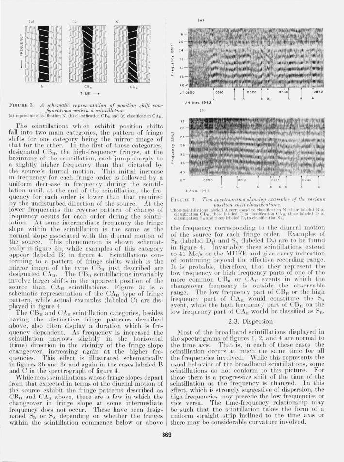
Many of the broadband scintillations observed show no measurable shift in position. Scintilla tions with this characteristic are referred to as N type scintillations in what follows . A schematic rep­resentation of this type of scintillation is shown in figure 3a while several of these scintillations (labeled A) are sho'wn in the spectrograms reproduced in figure 4.

868

(0 I ( bl

N CB,

TIME _

(e l

CA,

FIGURE 3 . A schematic representation of position shift con­figurations within a scintillation.

(a) represents classification N, (b) classification CBII and (c) classiFIcation CAn.

The scintillations which exhibit position shifts fal.l into two main categories, the pattern of fringe shIfts for one category being the mirror image of tha.t for the other. In the first of these categories, deslgnated CB[[, thc higb-frcquency {rino·es at the begi?-ning of the scintillation, each jump bsh~rply to a slIghtly higiler frequency tball that dicta,ted by the source's diurnal motioJl. TJ1is initial iocrcase in .frequency for each fringc order is followed by a umform deer·ease in freq uen cy during the scin til­lation until, at the end of the sci ntillation, the fre­quency for each order is lower than that required by the undisturbed direction of the source. At the lower frequencies the reverse pattern of change of frequency occurs for eacl1 order durin o· the scin til­lation. At some intermediate frequen~y the fringe slope within the scintillation is the same as the normal slope associated with the diurnal motion of the source. This phenomenon is shown schemat­ically in figure 3b, while examples of this category appear (labeled B) in figure 4. Scintillations con­fo~·ming. to a, pa,ttel'l1 of fringe shifts which is the mH·.ror lmage of the type CBH just described are deslgnated CAn. The CBn scintilla,tions invariably involve la,rger shifts in the apparent position of the source than CAn scintillations. Figure 3c is a schematic r~presentation of the CAH type of fringe pattern, wlllle actual examples (labeled C) are dis­played in figure 4.

The CBH and CAn scintillation categories, besides having the distinctive fringe patterns described above, also often display a dmation which is fre­quency dependent . As frequency is increased the scintillation narrows slightly in the horizontal (time) direction in the vicinity of the fringe slope changeover, increasing again at the higher fre­quencies. This effect is illustrated schematically in figures 3b and 3c and again in the cases labelf'd i3 and C in the spectrograph of figme 4.

While most scintillations whose fringe slopes depart from that expected in terms of the diurnal motion of the som ce exhibit the hinge patterns described as CBH and CAn above, them are a, few in which the changeover in fringe slope at some intermediate frequency does not occur. These have been desig­nated Sn or SA depending on whether the fringes within the scintillation commence below or above

(0 I

(b I

,. 20

I 2 4 ~ ~ 2. c ~

>2 ~

... 36

40

UT

3 AUQ . 1962

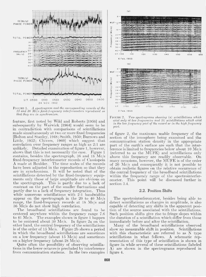
FIG URE '1. Two spectrograms showing examples of the l'(l1· i01IS position shift classificat·ioll s.

'f]10SC scintill ations labeled A correspond to cl ass ificatioll ;\ , t ilO i l ' la lw ll'd n to classification C B/I , th ose iai)C' \cd C to class ifica tion CAli , Lho3C labeled I) to c lassificat ion Su a lld t hose labeled D2 to class ification SA.

tbe frequency corresponding Lo Lhe diurnal moLion of the source for each fringe order. Examples of

n (labeled D 1) and SA (hbeled D z) are to be found in figure 4. In variably t he e scintillations extend to 41 Mcls or t he MUFE and gil'e every indication of continuing beyond the effective recording range. It is probable, tbere[ore, that t l1ey represent tbe low frequency or high frequency parLs of one oC t he more common CBn or CAll events in which t he changeover frequency is ouLside the obsOlTable range. The low frequency part of CBn or the high frequency part of CAlI would constitute the SA event, while the high frequency part of CBH on the low frequency part of CAlI woulcl be classified as Sn.

2.3. Dispersion

Most of the broadband scintillations displayed in the spectrograms of figures 1, 2, and 4 are normal to the time axis. That is , in each of these cases, the scintillation occurs at much the same time for all the frequencies involved. While this represents the usual behavior of the broadband scintillations, some scintillations do not conform to this picture. For these there is a progressive shift of the time of the scintillation as the frequency is changed. In this effect, which is strongly suggesti ve of dispersion, the high frequencies may precede the low frequencies or vice versa. The time-frequency relationship may be such that the scintillation takes the form of a uniform straight strip inclined to the time axis or there may be considerable curvature involved.

869

(a I

( bl

12-

"-

:>

~ ~ ~ ~

u.

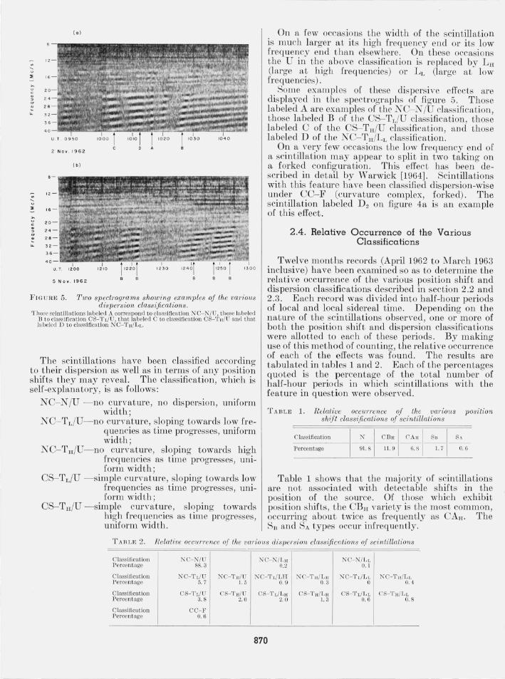
FIGURE 5. Two spectrograms showing examples of the various dispeTsion classifications.

'ThOEC Ecintilia tions la boled A correspond to classification N C- N/U, those labeled B to clascification CS- 'rL/ U, that labeled C to classification CS-TH/U and that labeled D to classification KC- TH/LL.

The scintillations have been classified according to their dispersion as well as in terms of any position shifts they may reveal. The classification, which is self-explanatory, is as follows:

NC- N IU - no curvature, no dispersion, uniform width;

NC-TL/U- no curvature, sloping towards low fre­quencies as time progresses, uniform width;

KC-TH/U- no curvature, sloping towards high frequencies as time progresses, uni­form width'

CS-TdU - simple curvat~re, sloping towards low frequencies as time progresses, uni­form width;

CS- TH/U -simplE' curvature, sloping towards high frequencies as time progresses, uniform width.

On a few occasions the width of the scintillation is much larger at its high frequency end or its low frequency end than elsewhere. On these occasions the U in the above classification is replaced by LH (large at high frequencies) or LL (large at low frequencies) .

Some examples of these dispersi \Te effects are displayed in the spectrographs of figure 5. Those labeled A are examples of the NC- N IU classification, those labeled B of the CS- TL/U classification, those labeled C of the CS- T H/U classification, and those labeled D of the NC- TH/LL classification.

On a very few occasions the low frequency end of a scintillation may appear to split in two taking on a forked configuration. This effect has been de­scribed in detail by Warwick [1964]. Scintillations with this feature have been classified dispersion-wise under CC-F (curvature complex, forked). The scintillation labeled D 2 on figure 4a is an example of this effect.

2.4. Relative Occurrence of the Various Classifica tions

Twelve months records (April 1962 to 'March 1963 inclusive) have been examined so as to determine the relative occurrence of the various position shift and dispersion classifications described in section 2.2 and 2.3 . Each record was divided into half-hour periods of local and local sidereal time. Depending on the nature of the scintillations observed, one or more of both the position shift and dispersion classifications were allotted to each of these periods. By making use of this method of counting, the relative occurrence of each of the effects was found. The results are tabulated in tables 1 and 2. Each of the percentages quoted is the percentage of the total number of half-hour periods in which scintillations with the feature in question were observed.

TABLE 1. R elative OCCU1Tence of the various position sh(ft classifications of scintillations

Table 1 shows that the majority of scintillations are not associated with detectable shifts in the position of the source. Of those which exhibit position sbifts , the CBH variety is the most common, occurring about twice as frequently as CAH. The SB and SA types occur infreqnently.

TARLE 2. Relative OCC11rTence of the various dispersion classifications of scintillations

C lassi ncation SC- N /U NC-""/LH I NC- N /LL Percentage 88.3 0.2 0. 1

Classificat ion NC- TL/U NC- TH/U ,,"C- T d Ll1 I NC- Tn/ Ln NC- TL/L L NC- TH /LL Percentage 5.7 1. 5 O. 9 0.3 0 0.4

Classificaiion CS- TL/U CS- TH/U CS- T L/Ln CS- T,.r/LH CS- TL/L L CS- TH/LL Percentage 3.8 2.0 2. 0 1.3 O. G 0.8

Classification CC- 1' Percentage 0. 6

870

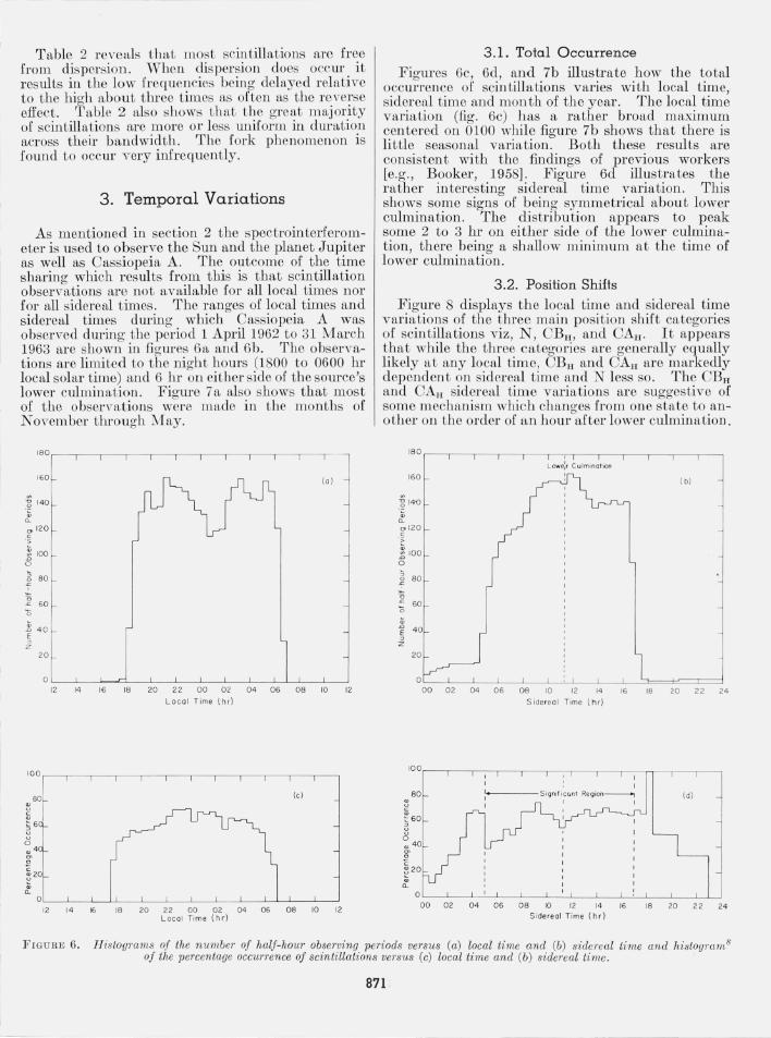
Table 2 re\Teals that most scintillations are free from dispersion. vVhen dispersion does occm it results in the low frequencies being delayed relative to the high about three times as often as the reverse effect. T able 2 also shows that the great majority of scintillations are more or less uniform in duration across their bandwidth. The fork phenomenon is found to occm very infrequently.

3. Temporal Variations

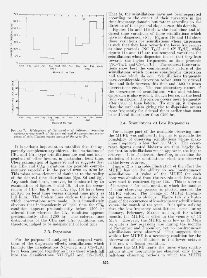
As mentioned in section 2 the spectrointerferom­eter is used to observe the Sun and the planet Jupiter as well as Cassiopeia A. The outcome of the time sharing which results from this is that scintillation observations are not available for all local times nor for all sidereal times. The ranges of local times and sidereal times dming which Cassiopeia A was observed during the period 1 April 1962 to 31 March 1963 are shown in figmes 6a and 6b . The observa­tions are limited to the night hours (1800 to 0600 hI' local solar t ime) and 6 hI' on ei ther side of the sOUTce's lower culmination. Figure 7a also shows that most of the obsenTations were made in the months of November through May.

180

160

~ ·0 140 .2 ~

Q.

g'120 ., .,

100 ~ .0 0

~ 80 0 ~ , :g 60 '0

1: 4 0 ~ z

20

g 80

~6 u o

~4

~20 Q.

(0 )

12 14 16 18 20 22 0 0 02 04 06 08 10 12

Lo ca l Time (hr)

(c)

12 14 16 18 20 22 00 0 2 04 06 08 10 12 Loc ol Time ( hr)

3.1. Total Occurrence Figures 6c, 6d, and 7b illustrate how the total

occurrence of scintillations varies with local time, sidereal time and month of the year. The local time variation (fig . 6c) has a rather broad maximum centered on 0100 while figure 7b shows that there is little seasonal variation. Both these results are consistent with the findings of previous workers [e.g., Booker, 1958]. Figure 6d illustrates the rather interesting sidereal time variation. This shows some signs of b eing symmetrical about lower culmination . The distribution appears to peak some 2 to 3 hI' on either side of the lower culmina­tion, there being a shallow minimum at the time of lower culmina tion.

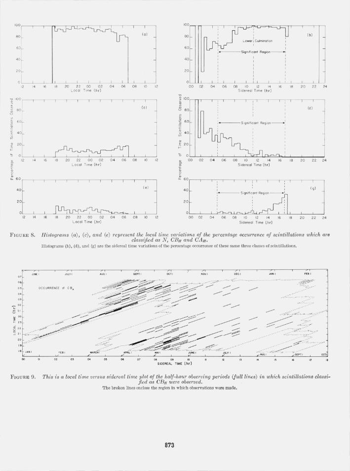
3.2. Position Shifts Figure 8 displays the local time and sidereal time

variations of the three main position shift categories of scintillations viz, N, CB H , and CAu. It appears that while the three categories are generally equally likely at any local time, CB H and CAn are markedly dependent on sidereal time and N less so. The CBu and CAlf sidereal time variations are suggestive of some mechanism which changes from one state to an­other on the order of an hour after lower culmination.

180 ,--,---,--,--, __ -.-,,'-__ r--' __ '-__ '--' __ ~

Lowe:r Culmlnalion

16 0

~ 140 .,

Q.

g'120

. ~

~ 100 o ~

80 2

2 60 0 ., .0 4 0 ~ z

( bl

02 04 06 08 10 12 14 16 18 20 2 2 24

Sidereal Time ( hr)

00 02 04 06 08 10 12 14 16 18 20 22 24 Sidereol T ime ( hr)

FIGURE 6. H istogmms of the n umber of half-hour observing periods versus (a) local ti me and (b) sidereal ti me and histogmmS

of the percentage occurrence of scintillations versus (c) local time and (b) sidereal time.

871

(f) z

600

~ 500

~ > ffi 400 if) (Il

0 300 t.-O

ffi 200 (Il

::!' ~ 100

(01

OL--i __ -L __ l-~ __ -L __ i-__ ~~ __ ~ __ L-~ __ ~ April May June July Aug Sept Oct Nov Dec Jon Feb March

1962 1963

Month of the Year

~IOO'--'---r--~--'--'--'---r--'---'--'--'--, z ~ (W a: => u g 60

w ~ 40 z w ~ 20 w CL

OL-~ __ -L __ ~~~-L __ ~ __ L-~ __ ~ __ L-~ __ ~

Ap ril May June July Aug Sept Oct Nov Dec Jan Feb March

1962 1963 Month of the Year

FIGU RE 7. H istogmms of the number of half-how' observing periods versus month of the year (a) and the percentage OCCUI'­

l'ence of scintillations versus month of the year (b).

It is perhaps important to establish that the ap­parently complementary sidereal time variations of CBH and CAH type scintillations are real and inde­pendent of other factors, in particular, local time. Close examination of figures 8c and 8e suggests that the CBH and CAH variations are possibly comple­mentary especially in the period 0200 to 0700 hr. This raises some element of doubt as to the reality of the sidereal time distributions (figs. 8d and 8g). Any such doubt can, however, be eliminated by an examination of figures 9 and 10. Here the occur­rences of CBH (fig. 9) and CAH (fig. 10) have been plotted on local time versus sidereal time plots as full lines. The broken lines enclose the period in which observations were made. It is immediately obvious that independently of local time the CBH condition appears predominantly before 1200 hI' sidereal time whereas the CAH condition appears predominantly after 1200 hr. The sidereal time distributions of the CBH and CAH conditions are, therefore, judged to b e independent of local time.

3.3. Dispersion

For the purpose of studying the temporal varia­tions of the dispersion effects, scintillations which fall into the classifications NC- TL/U and CS- TL/U have been lumped together as have those which fall into the classifications NC-TH/U and CS-TH/U,

That is, the scintillations have not been separated according to the extent of their curvature in the time-frequency domain but rather according to the direction of their general slope across this domain.

Figures lla and lIb show the local time and si­dereal time variations of those scintillations which have no dispersion (N). Figures llc and lId show these variations for scintillations whose dispersion is such that they lean towards the lower frequencies as time proceeds (NC- TL/U and CS- TL/U), while figures lIe and llf are the temporal variations for scintillations whose dispersion is such that they lean towards the higher frequencies as time proceeds (NC-T H/U and CS- T H/U), The sidereal time varia­tions show best the complementary nature of the scintillations which possess considerable dispersion and those which do not. Scintillations frequently have considerable dispersion before 0900 hr sidereal time and little between this time and 1600 hI' when observations cease. The complementary nature of the occurrence of scintillations with and without dispersion is also evident, though less so, in the local time variations. Dispersion occurs more frequently after 0200 hr than before. To sum up, it appears that the mechanism giving rise to dispersion occurs more frequently for sidereal times earlier than 0900 hI' and local times later than 0200 hr.

3.4. Scintillations at Low Frequencies

For a large part of the available observing time the MUFE was sufficiently high as to preclude the possibility of observing scintillations whose maxi­mum frequency is less than 20 Mc/s. The occur­rence figures quoted hitherto are thus largely de­pendent on scintillations which appeal' in the higher octaves. It is of interest, therefore, to examine the statistics of those scintillations which are observed in the lower octaves.

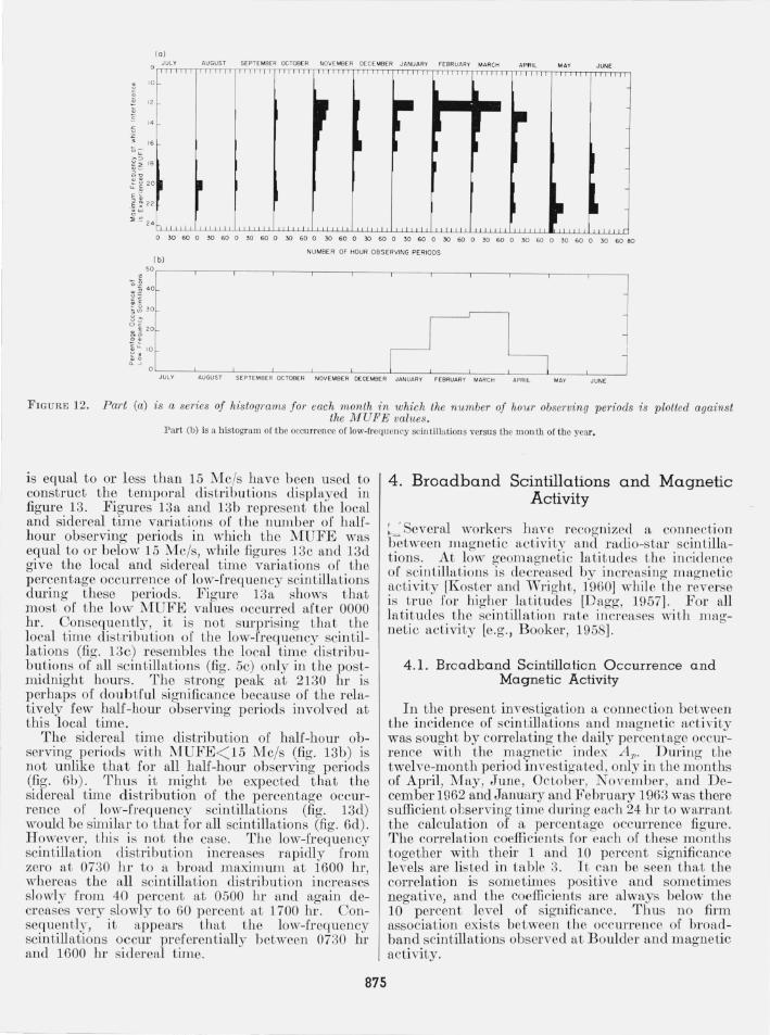
Figure 12 is a graphic illustration of the effect the MUFE has on the ability to see low-frequency scintillations. A value of the MUFE for each hour was obtained from the records and these data were used to construct figure 12a. This is a series of histograms for each month in which the number of hour observing periods is plotted against the MUFE values. The change of MUFE through­out the seasons is obvious. Figure 12b is a histo­gram of the occurrence of low-frequency scintillations versus the month of the year. It is quite striking that the low-frequency scintillations occur during January, February, March, and April for which months the MUFE is often in the vicinity of 13 Mc/s. However, the MUFE is as low as 13 Mc/s on quite a few occasions also during the months of November and December, yet no low-frequency scintillations were observed. This suggests that while a low MUFE is a necessary condition for the observation of scintillations in the lower octaves it is not a sufficient condition.

Since the MUFE limits the times when scintil­lations at low frequencies are observed, only those half-hour observing periods in which the MUFE

872

100

80

"l 40

20

0 12 14

"0 100 w > w

0 80_ 0 ! ~ c 60 0

~ C 4 0 U if)

~ 20

l-

'5 0 w '2 ,4 ry 0

c w u w "-

:1 :

'2 '4

FIGURE 8.

0 7

05

o.

0' _ 02

.:; 0 I

w 00 ~

i= 2 3

-' ~ 22 o -,21

20

,. "

00

100

(01 ,

( bl 80 , I

Lower I Culminat ion I

6 0 Si gn ificant Region-I

I

4 0

20

0 16 18 20 22 00 02 04 06 08 10 ,2 00 02 0 4 06 08 '0 '2 '4 '6 '8 20 22 24

Loc al Time (hrl Sidereal Time (h r l "0 fOO I

, I

(cl (d I 0 80 ~

.§ 60 Signi ficant Region-: 0

"" c u 4 0 if)

E 20 I-

'5 0

'6 '8 20 22 00 02 0 4 0 6 08 '0 '2 w 00 02 0 4 0 6 08 '0 '2 '4 '6 '8 20 22 24 Loc ol Time (h r l

ry Si de real Time (hr) 0

c w u w "- 60

I

~ : ' ~,

j 4 0 I ( gl

" Significant Reg ion_I ,

20

0 ,6 ,8 20 22 00 02 04 06 08 '0 ,2 00 02 0 4 06 08 '0 '2 ,4 '6 '8 20 22 24

Loco, Time (h r) Side real Time (h r)

Histograms (a), (c), and (e) represent the local lime variations of the percentage occurrence of scintillations which are classified as N, CBn and CAn.

Histograms (h), (d), and (g) are the sidereal time variations of the percentage occurrence of these same three classes of scintillations.

AUG 1 SEPT. I OCT! NOV. I DEC.' fEB. '

OCCURREN CE of CB H

----:.j~.!:tt~ ... '-'i'~~~"" .' .- .. -

fEB I JULY I

0' 02 0' o. 0' 06 07 09 10 12 " S'OEREAL T'ME (hr)

FIG URE 9. This is a local time veTSUS sidereal time plot of the half-hour obseTving periods (full lines) in which scintillations classi­fied as CBn were observed.

The broken lines en close the region in whieh observations were made.

873

0 ' ~--~7'-E',------r---J7UL-Y"------'----ArUG"------'----S~E~PIr. -----,----.Oc~yrl ------r---~.O~V~. I-----,----:O:EC:. ~, -----.----·JA~.r. l------.----:.FE=.r. I ----~ 07

06

0' O'

w " 01 ;:

00 -' .. un o -' "

20

" "

... :.-:

00

OCCURRENCE 01 C AH

..... - ... . ...... ... --

FEB.I MARCHI

01 0 2 0'

... ,.

...... !:; :: . . .. ,-

APRil I

'" 06 07 08 O' 10 12 " " I. 17 " SIDEREAL TIME lhr)

F I GURE 10. This is local ti me versus sidereal time plot of the half-hour observing periods (fu ll lines) in which scintillations classi~ fied as CA H were observed.

The broken lines enclose the region in which observations wore made.

100 100

8 0 ( 0 )

8 0 (bl

6 0 60

40 40

20 20 0

0 w

w > > 0 0:: 0 0:: W w 12 14 16 18 20 22 00 02 0 4 0 6 0 8 10 12 V> 00 02 04 06 08 10 12 14 16 :8 20 2 2 24 CJ1 CD CD Local Time (hr) 0 Side real Time (hr ) 0

CJ1 ~ 100 z 100

<::> <::> I--

I-- (c ) <{ (d ) <{ 80 -' 80 -' -' -' ;:: I--

6 0 "" 6 0

"" u

u V> ;-Sig ni f icont Reg ion-: V>

1

W 4 0 w 40 ::; ::;

I--;:: IL

20 IL 20 0

0

w w 0 '" 0 '" 12 14 16 18 08 10 12 <{ 00 0 2 0 4 06 08 18 20 22 24 <{

I--I--Loc ol Tim e ( hr ) z Si dereal Time (h r ) z w w u U

0:: 0:: UJ W

"-

:~f "-

:~f : : .~~ : '~' ~ ~l~'

, I

,,;

J o CJ 12 14 16 18 2 0 22 0 0 02 04 0 6 0 8 10 12 00 02 04 06 0 8 10 12 14 16 18 20 22 2~

Loc al Ti me (hr) Si dereal Time ( hr )

F IGURE 1] . Histograms (a), (c), and (el re presf-nt the local time variations of the percentage occurrence of scinti llations which are classified as NC-N/U, NC- and CS-TL/ U and NC- and CS- TH /U.

Histograms (b) , (d), and (f) are tbe sielereal time var iations of tbe percen tage occurrence of these same th ree classes of scintillations.

874

(a) JULY AUGUST SEPTE MBER OCTOBER NOVEMBER DECE MBER JANUARY FEBRUARY MARCH APRIL MAY JUNE , l1li

• l I ~ 14

• I a.

- l r o 30 60 0 30 60 0 30 60 0 JO 60 0 30 60 0 30 60 0 30 60 0 30 60 0 30 60 0 30 60 0 30 60 0 30 60 80

NUMBER OF HOUR OBSERVING PERIODS ( b)

JULY AUGUST SEPTEMBER OCTOB ER NOV EMBER DECE MBER JANUARY FEBRUARY MARCH APRIL MAY JUNE

FIGU RE 12. Part (a) i s a series of his tograms for each month in which the number of hour obsel'ving periods is plotted against the M UFE values .

Part (b) is a histogram of the occurrence of low-frequency scintillations versus the month of the year.

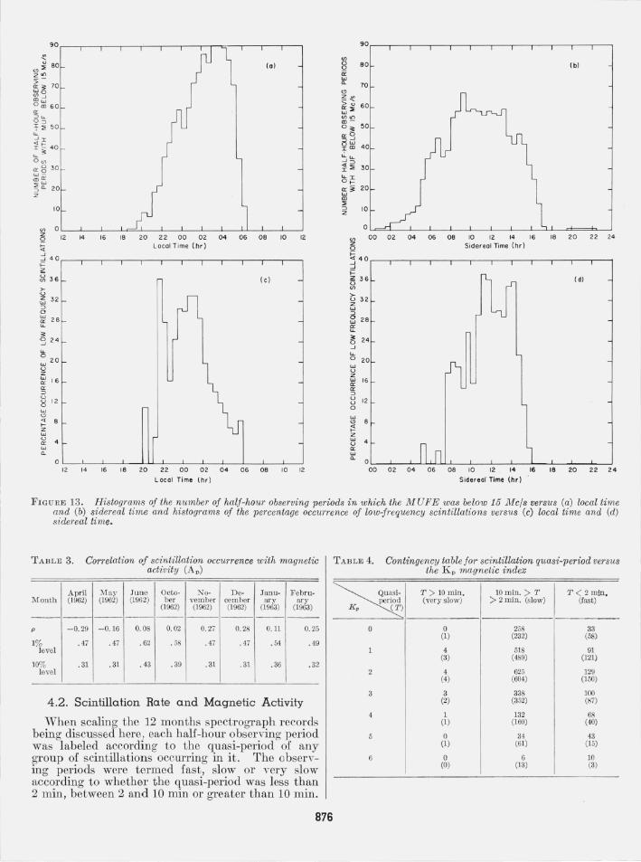
is equal to or less than 15 Mc/s havc been used to construct the temporal distributions displayed in figure 13. Figures 13a and 13b represent the local and sidereal time variations of the number of half­hour observing periods in which the MUFE was equal to 01' below 15 Mc/s, while figures 13c and 13d give the local and sidereal time variations of the percentage occurrence of low-frequency scin tillations during these periods . Figlll'e 13a shows that most of the low MUFE values OCCUlTed after 0000 hr. Consequently, it is not surprising that the local time distribution of the low-frequency scintil­lations (fig. 13c) resembles the local time clis tribu­butions of all scintillations (fig . 5c) only in the post­midnight hours . The strong peak at 2130 hI' is perhaps of doubtful significance because of the rela­tively few half-hour observing periods involved at this local time.

The sidereal time distribution of half-hour ob­serving periods with MUFE< 15 Mc/s (fig. 13b) is not unlike that for all half-hour observing periods (fig. 6b) . Thus it might be expected that the sidereal time distribution of the percentage occur­rence of low-frequency scintillations (fig. 13d) would be similar to that for all scintillations (fig. 6d). However, this is not the case. The low-frequency scintillation distribution increases rapidly from zero at 0730 hI' to a broad maA'imum at 1600 hI', whereas the all scintillation distribution increases slowly from 40 percent at 0500 hI' and again de­creases very slowly to 60 percent at 1700 hr. Con­sequently, it appears that the low-frequency scintillations occur preferentially between 0730 hI' and 1600 hI' sider eal time.

875

L_

4. Broadband Scintillations and Magnetic Activity

~~ Several workers ll ave recognized f\, connection between magneti c activity and radio- tar scintilla­t ions. At low geomagnetic latit udes the in cidence of scintillaLions is decreased by increasing magnetic activity [Koster and Wri gh t, 1960] while the reverse is true for higher latitudes [Dagg, 1957] . For all latitudes the scintillation rate increases with mag­netic activity [e.g ., Booker, 1958].

4.1. Broadband Scintillation Occurrence and Magnetic Activity

In the present investigation a connection between the incidence of scintillations and magnetic activity was sought by correlating the daily percentage occur­rence with the magnetic index A v. During the twelve-month period investigated, only in the months of April, :May, June, October, November, and De­cember 1962 and January and February 1963 was there sufficient observing time during each 24 hI' to warrant the calculation of a percentage OCCUlTence figure . The correlation coefficients for each of these months together with their 1 and 10 percent significance levels are listed in table 3. It can be seen that the correlation is sometimes positive and sometimes negative, and the coefficients are always below the 10 percent level of significance. Thus no firm association exists between the occmrence of broad­band scintilla tions obscrvcd at Boulder and magnetic activity.

80 (0 )

10

~ OLI2--~14--~16---,L8==~2-0--~22---0LO--~0-2--0~4---0L6L-~0-8--~'0--~'2 Q ~ Local Time (hrl -' ,g 4 0 ,--___,---,---,__--_,_--,__--,----___,--_,_--,__--_,_--,__---,

z g 36

>­u

,~ 32 :::l o ~ 28 "-

'" '3 2 4

"­o 20 w

u z ~ 16 er :::l

'~ 12 w

'" ;: 8 z w

.~ 4 w ,a.

12 14 16 18 20 22 00 02 Local Time l hr)

04

( c)

06 08 10 12

'" ~~

80

70

> (.) 60 5~ (f)<rl <D-0", 50 er o i3lil I CD 40

"-u. -':::l ~ ~ 30

~~ er j< 20 w <D ~

~ 10

(b)

OW=~ __ _L __ ~ __ L__L __ _L __ ~~L_~ __ d===~~

(f) 00 02 04 06 z o

08 10 12 14 16 Sidereal Time (hr)

18 20 22 24

i= ~40,---,---r---r---,---,---,-------,---,---,-----,---,--~

i= ~ 36 u (f)

>­u 32 z

3 w 28 [

~ 24 -' "­o 20 w u z ~ 16 a: :::l

~ 12 o w '" 8 ;'0 z w u er w

( d)

a. OL-~ __ _L-L~LU~ __ L_ __ L-~ __ ~ __ _L __ ~ __ ~~

00 02 04 06 08 10 12 14

Sidereal Time (hr)

16 18 20 22 24

FIGU RE 13. Histograms of the number of half-hour observing periods in which the MUFE was below 15 lVfc/s versus (a) local time and (b) lIidereal time and histograms of the percentage occurrence of low-f requency scintillations versus (c) local time and (d) sidereal time.

T A BLE 3. Correlation of scintillation occurrence with magnetic activity (A D)

April M ay June Octo- No· D e· Janu- Febru· Month (1962) (1962) (1962) ber vcmber cember ar y ary

(1962) (1962) (1962) (1963) (1963)

-- ----- --- - - -------- --------p - 0.29 - 0. 16 0.08 0.02 0.27 0. 28 0. 11 0. 25

1% . 47 . 47 .62 .58 .47 .47 . 54 . 49 level

10% . 31 .31 .43 . 39 .31 .31 .36 .32 level

4.2. Scintillation Rate and Magnetic Activity

When scaling the 12 months spectrograph records being discussed here, each half-hour observing period was labeled according to the quasi-period of any group of scintillations occurring in it. The observ­ing periods were termed fast, slow or very slow according to whether the quasi-period was less than 2 min, between 2 and 10 min or greater than 10 min.

876

TABLE 4. Contingency table for scintillation quasi-period versus the Kp magnetic index

~ T > 10 min. 10 m in . > T T < 2 min.

period (ver y slow) > 2 min. (slow) (fast) K p ( T )

0 0 258 33 (1) (232) (58)

1 4 518 91 (3) (489) (121)

2 4 625 129 (4) (604) (150)

3 3 338 100 (2) (352) (87)

4 1 132 68 (1) (160) (40)

5 0 34 43 (1) (61) (15)

6 0 6 10 (0) (13) (3)

A contingency table was then constructed for these three classes against the magnetic index K p. The result is shown in table 4. The numbers in brackets in the various cells of this table represent the number of events expected on the basis of a random distribu­tion. It will be noted that as Kp increases the ratio of the observed to the expected number of events increases for the fast scintillations but decreases for the slow scintillations. This suggests that the quasi­period is not randomly distributed with regard to magnetic activity but rather the quasi-period decreases with increasing magnetic activity. A chi-square test on the data of table 2 shows that the probability that the observed distribution is a random one is less th an 1 in 1000.

5. Broadband Scintillations and Ionospheric Conditions

It has long been realized that radio-star scintilla­tions and the ionospheric phenomenon oJ spread-F [Singleton, 1957] are related and probably have a common origin [Ryle and Hewish, 1950; Little and Maxwell, 1951]. Consequently, associations were sought between broadband scintillations and various properties of the ionosphere.

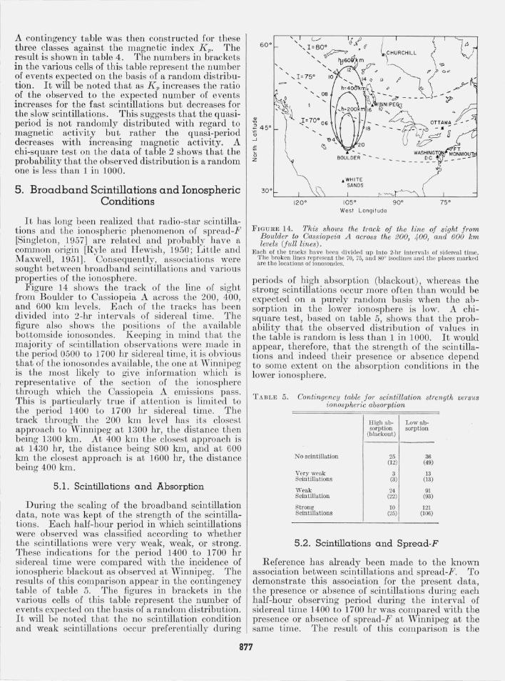
Figure 14 shows the track of the line of sight from Boulder to Cassiopeia A across the 200 , 400, and 600 km levels. Each of the tracks has been divided into 2-h1" intervals of sidereal tim e. The figure also shows the positions of the available bottomsid e ionosondes. Keeping in mind Lhat the majority of scintillation observations were made in the period 0500 to 1700 hI' sidereal time, it is obvious that of the ionosondes available, the one at Winnipeg is the most likely to give information which is representative of the section of the ionosphere through which the Cassiopeia A emissions pass. This is particularly true if attention is limited to the period 1400 to 1700 hI' sidereal t ime. The track through the 200 km level has its closest approach to Winnipeg at 1300 hI', the distance then being 1300 kIn. At 400 km the closest approach is at 1430 hI', the distance being 800 km, and at 600 kIn the closest approach is at 1600 ill, the distance being 400 km.

5.1. Scintillations and Absorption

During the scaling of the broadband scintillation data, note was kept of the strength of the scintilla­tions. Each half-hour period in which scintillations were observed was classified according to whether the scintillations were very weak, weak, or strong. These indications for the period 1400 to 1700 hI' sidereal time were compared with t he incidence of ionospheric blackout as observed at Winnipeg. The results of this comparison appear in the contingency table of table 5. The figm es in brackets in the various cells of this table represent the number of events expected on the basis of a random distribution. It w·ill be noted that the no scintillation condition and weak scintillations occm preferentially dming

,:: (; z

.... , .... ....

1050

West Longitude

FIGURE 14. This shows the tTack of the line of sight fTom Boulder to Cassiopeia A across the 200, 400, and 600 km levels (fu ll lines) .

Each of the tracks have been divided up into 2·hr intervals of sid ereal t ime. 'rhe broken lines represen t t he 70, 75, and 800 isoclincs a nd tbe places m arked a rc tbe locations of ionosondcs.

periods of high absorption (blackout), whereas the strong scintillations occur more often than would be expected on a pmely random basis when the ab­sorption in the lower ionosphere is low. A chi­square test, based on table 5, shows that the prob­ability that the observed distribution of values in the table is random is less than 1 in 1000. It would appear, therefore, that the strength of the scintilla­tions and indeed their presence or absence depend to some extent on the absorption conditions in the lower ionosphere.

TABI,E 5. Contingency table for scintillation strength veTSUS ionospheTic absorption

lligb abo Low abo sorption sorption

(blackout)

No scintillation 25 36 (12) (49)

Very weak 3 13 Scintillations (3) (13)

Weak 24 91 Scintillation (22) (93)

Strong 10 121 Scintillations (25) (106)

5.2. Scintillations and Spread-F

Reference has already been made to the known association between scintillations and spread-F. To demonstrate this association for the present data, the presence or absence of scintillations during each half-hour observing period during the interval of sidereal time 1400 to 1700 hI' was compared with the presence or absence of spread-F at Winnipeg at the same time. The result of this comparison is the

877

contingency table of table 6. The figures in bracket" in the vari ous cells of this table represent the number of events expected on the basis of a random distribu­tion. The t endency for scintillations and spread-F to be present or absent at the same time will be noted. A chi-square test , based on t able 6, shows that the probability that the observed distribution of events in the t able is random is less than 1 to 1000.

T ABLE 6. Contingency tah le f or sp?'ead-F occurren ce V"TSUS scinti llation OCCUT1'( nCe

~ Sprcacl·P NO Y E S

;~ Scin t illa-tions occ-urring

NO 22 14 (7) (29)

YE S :jO 201 (45) ( 186)

It is also instructive to examine the possibility that the severity of the scintillations is related to the severity of the accompanying spread-F. In this comparison the strength of the scintillations was taken as a measure of its severity, whereas the frequency extent (oj) of the spread-F configuration [Singleton, 1962] was used as a measure of its severity. The contingency table resulting from this comparison is shown in table 7. Again the numbers in brackets are the numbers of events expected in the various cells on the basis of a purely random distribution. It will be noted that nowhere is the observed number of events significantly different from. the number expected on the basis of a random distribution. Indeed, a chi-square test on this table shows that the probability that the observed distribution is a random one is better than 0.99. It would appear, therefore, that there is little or no association between the severity of scintillations and the associated spread-F.

T ABLE 7. Conti ngency table fo r scintillation stren gth vel'SUS Ih e severity of s pread-F (0 f 0)

~ ........ oj , 0.2 0.3 0.4 0.5 0.0 O.i 0.8

Sciniilla-~ tion stren gth

----,---- "-- - - - -No 4 0 I 2 1 0 0

scintillation s (6) (4) (2) (2) (I) (0) (0)

Very weak 3 3 0 0 0 0 0 sci n ti lla tions (3) (2) (I ) (1) (0) (0) (0)

Weak 31 19 10 8 3 2 2 sci ntillations (31) (20) (9) (8) (4 ) (1) (2)

Strong 47 '27 J4 12 0 0 2

scinti llation'.:: (45) (29) , ( 13) (1 1) (5) ( I ) (2)

Warwick [1964] has suggested that the changeo\TBl' in the fringe pattern of scintilla tions of th e CEIl and CAH types is the result of the focusing action of the ionospheric lenses which, he suggests, are responsible for the broadballd scintillations. The association between the occurrence of spread-F and

scintillations suggests that these lenses may be the same ionospheric irregularities as give rise to the spread-F echoes.

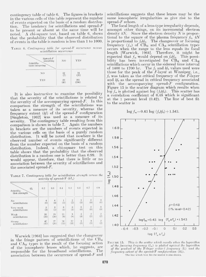
The focal length of a lens-type irregularity depends amongst other things, on its incremental electro~ density oN. Since the electron density N is propor­~ional to the square of the plasma frequency j a, oN IS proportional to j~oj~. The changeover or focusing frequency (j",) of CEn and CAH scintillation typei=' occurs when the range to the lens equals its focal length [Warwick, 1964]. Therefore, it might be expected that j m would depend on j oojo. This possi­bility has been investigated for CEn and CAH

scintillations which occur in the sidereal time interval of 1400 to 1700 hr. The j a and ojo values used were those for the peak of the F-layer at Winnipeg, i.e., j o was taken as the critical frequency of the F-layer and ojo as the spread in critical frequency associated with the accompanying spread-F configuration. Figure 15 is the scatter diagram which results when log j m is plotted against log (Jaoja). This scatter has a correlation coefficient of 0.48 which is significan t at the 1 percent level (0.42). The line of best fit to the scatter is

1.6 0

1.58

1. 56 . . 1.5 4 ... 1. 52

E .... 1.50

01 0 .. 0

1.48 . . 1.46

1.44 p=0.48

(1% level=0.42)

1.42

1.40 -0.4 -0.3 -0.2 -0. i 0 0.1 0.2 0.3

FIC UHE 15. This is the Bcatte?' which Tesu lts when the lugarith m of the f ocusing freq1ten cy (f m) is plottcd against the 10gG?'ith m of the pToduct of the F -layer criticci frequency (fo) and the f Teq1lency extent of the spread-F config uration (Mo).

'I'h e line wh ich best fi ts the scatter is a lso shown .

878

This suggests that ./,! is proportional to .1011./0, the constan t of propor tionali ty being in the vicini ty of 1.2X 103. Thus broadband scin t illations, besides occurring at th e same t ime as spread-F, are r elated in a simple way, t hrough their focusing Ireq uency, to the par ameters of the spread-F configuration.

6. Conclusions

The main conclusion to be drawn from this statistical investigation of 12 months observations of the scin tillations of Cassiopeia A made with the Boulder spectrointerferometer are as follows.

(1) The scintillations observed are broadband centered anywh'3r e in t he frequency range of 7.6 to 41 M c/s. Bandwidths of 2:1 are common . H ow­ever , bandwidths as high as 4: 1 are encountered very r arely.

(2) The occurrence pattern of t he scin tillations, while varying little wit h season, is markedly de­penden t on local and sidereal time. The local t ime varia tion has a broad maximum cen tered on 0100 , while t he sidereal t ime variation peaks so me 2 to 3 hr on either side of a minimum at the t ime of lowor culmination.

(3) Besides in vol ving cllanges in signal stre ngth some scin tillations are associated wit h changes in t he apparen t p osition of t he source . There are t wo main position shif t configurations which are mirror images of each other . Each of t hese co nfigurations implies an ini tisl sudden shif t in the apparent position of the source followed by a gradual recovery to and overshoot of t he original source position and a final sudden shift back to t he undisturbed position of t he sourcc. The sense of the initial shif t, reco \'ery, etc., reverses fl,S frequency is increased , t here being an intermediate frequency at which t here is appar­ently no posit ion shift . Scintillations associated with position s bif ts while OCCUlTing with equal like­lihood at any l ocal time have an occurrence pattern which is markedly depende nt on sidereal t ime. The CBH type occurs mainly before 1200 hI'sidereal t ime, while t he CAn type occurs mainly after this t ime.

(4) Most scintillations are free f rom dispersion. H owever , for s ome scintillations the low frequencies are delayed relative to t he high , while for others t he reverse is the case. Dispersion occurs for sider eal times earlier than 0900 hI' and local times la ter than 0200 hr.

(5) The occurrence of scin till ations does not correlate wit h m agnetic activity. H owever, the quasi-period of gro~ps of. s.cint!llations is found to decrease as magnetIC actIVIty lllcreases.

(6) The occurrence of scintillations correlates positively with the occurrence of spread-F as ob­sened on a n earby ionosonde. The severity of the scintillatio ns, however , does not seem to be related to the severity of the associated spread-F . The focusing frequency of the scin tillations which exhibit posi tion shif ts is found to be related in a simple way to the parameters of the associated spread-F coniigUl'ation.

879

Par t II of this series will co nsider the exten t to which t hese obser vations can be explained by t he refracti \Te proper ties of the ionospheric irregularities which are believed to give rise to the broadband scintillations.

It is wi t h pl easure that the au thor acknowledges the use of t he facilities afforded him by t he High Alt itude Obsen Tatory to carry ou t the work repor ted her e while on sabbatical leave from the University of Queensland. In particular , he would like to thank Dr. J ames W . Warwick of t he Observatory staff who suggested the ilwestigation and maintained a very active interest in it .

The research reported here was s ponsored , in par t, by t he Ail' Force Cambridge R esearch Lab­oratories.

7. References

Aarons, J . (1963), Rad io Astro nomical and Satclli tc Stud ics of t hc Atmosphcrc (N ort h-H olla ncl ])u b. Co., Amstcrda m).

Bo ischot, A., R . H . Lcc, a nd J. W. Wa rwick (1960) , LolV­frcq ucncy so la r bursts a nd no isc sto rms, Astrophys. J . 131, 61- 7'1.

Bo lto n, J . G., and G . J . Stanlcy (1948), Obscrvat ions on t he va riable source of cos mi c rad io fr eq ue ncy rad iat ion in t he constellat ion of Cygnus, Aus tra lia n J . Sc i. Res. lA, 58- 69.

Booker, H . U. (1958), T hc usc of rad io stars to s t udy irregula r rcfract ions of rad io wav es in t hc ionosphe re, Proc. IRE 46, 298- 314.

Bur rows, K., and C . G. Littlc (1952), Simul ta neous obser­vatio ns of rad io star scint illat ions on t \\·o widcly spaced frequcncics, J od rcll Bank Annals 1, 29- 3.5.

Chi vcrs, H . J. A. ( 1960) , T he s imulta neo us observat ions of rad io sta r scint illat ions of differcnt r ad io-f rcquencies, J . Atmospheric T eJ'l'cst. Phys. 17, 181- 187.

Dagg, '\Ie (1957), T he correlat io n of radio-star-scint illat ion phenom ena wit h gcomagnet ic d ist urballccs a nd th c mccha­nism of motion of th e ion osphcric ir regularit ics in thc F region, J. Atmosphcr ic Tel'l'cs t . Phys. 10, 194- 203 .

Kostcr, J. H.., and R. W. Wright (1960), Scin t illatio n, spread F a nd t ranseq uatot'ia l sca ttcr, J . Gcophys. Res. 65, 2303- 2306.

Lec, H.. H ., a nd J . W. Wa rwick ( 1964·) , A spect rographi c in terfcromctcr, Rad io Sci. J . R es. N BS/ USNC- URSI 68D, No.7 807- 8 11.

L ittlc, C. G., and A. Maxwell (1951), F luct uations in th c in­t cnsity of rad io \Va "cs from galactic sources, Phil. ::VIag. 42, 267- 278.

Rylc, M ., a nd A. H C\\' ish (1950), Th e efl' ects of t he te rres t ria l ionosphcre on the rad io waves from d iscrete sources in t he 'galaxy, Monthly Not. Roy . Astrom. Soc. 110, 381- 394.

Singleton, D. G. (1957) , A st udy of "sp read-fi''' ionosphere ech oes at n ight at Brisba ne, III. Frcq uency spread in g, Austral ian J . Phys. 10, 60- 76.

Singleto n, D . G. (1962), Spread-F and the per t urbations of t he maxim.um electron dens ity of th c F lay er, Aust ra lian J. Phys. 15, 242- 260.

Smit h, F. G. (1950), Origin of thc fluctuations in the i ntensity of r adio waves from galact ic sources, Natllt'e 165, 422- 423 .

Warwick, J . W. (1961), Thcory of Jupi ter's decametri c emission, An nals New York Acad emy of Sciences 95, 39- 60 .

Warwick, J . W . (1963) , D ynam iC spcctr a of Jupi ter ' s deca­metric emission, 1961, Astrophys. J . 137, 41- 60.

Warwi ck , J. W . (1964), Rad io-star scintillations from iono­spheri c waves, R ad io Sci. J . R es. NBS/USNC- UUSI 68D, N o.2, 179- 188.

Wild , J . P. , and J . A. R ober ts (1056), The spectrum of rad io­star scint illations and t hc natu re of i neq uali t ies in t he ionospherc, J . Atmosphcr ic T Cl'l'es t. Ph ys. 8, 55- 75.

(Paper 68D8- 385)