Identifiability of Nonparametric Mixture Models and Bayes

Optimal Clustering

Bryon Aragam Chen Dan Eric P. Xing Pradeep Ravikumar

February 19, 2020

Abstract

Motivated by problems in data clustering, we establish general conditions under which families ofnonparametric mixture models are identifiable, by introducing a novel framework involving clusteringoverfitted parametric (i.e. misspecified) mixture models. These identifiability conditions generalize ex-isting conditions in the literature, and are flexible enough to include for example mixtures of Gaussianmixtures. In contrast to the recent literature on estimating nonparametric mixtures, we allow for generalnonparametric mixture components, and instead impose regularity assumptions on the underlying mixingmeasure. As our primary application, we apply these results to partition-based clustering, generalizingthe notion of a Bayes optimal partition from classical parametric model-based clustering to nonpara-metric settings. Furthermore, this framework is constructive so that it yields a practical algorithm forlearning identified mixtures, which is illustrated through several examples on real data. The key concep-tual device in the analysis is the convex, metric geometry of probability measures on metric spaces andits connection to the Wasserstein convergence of mixing measures. The result is a flexible framework fornonparametric clustering with formal consistency guarantees.

1 Introduction

In data clustering, we provide a grouping of a set of data points, or more generally, a partition of theinput space from which the data points are drawn [33]. The many approaches to formalize the learning ofsuch a partition from data include mode clustering [20], density clustering [56, 61, 63, 64], spectral clustering[52, 59, 76], K-means [49, 50, 62], stochastic blockmodels [3, 26, 39, 58], and hierarchical clustering [18, 34, 71],among others. In this paper, we are interested in so-called model-based clustering where the data points aredrawn i.i.d. from some distribution, the most canonical instance of which is arguably Gaussian model-basedclustering, in which points are drawn from a Gaussian mixture model [7, 23]. This mixture model canthen be used to specify a natural partition over the input space, specifically into regions where each of theGaussian mixture components is most likely. When the Gaussian mixture model is appropriate, this providesa simple, well-defined partition, and has been extended to various parametric and semi-parametric models[11, 27, 74]. However, the extension of this methodology to general nonparametric settings has remainedelusive. This is largely due to the extreme non-identifiability of nonparametric mixture models, a problemwhich is well-studied but for which existing results require strong assumptions [14, 42, 44, 70]. It has been asignificant open problem to generalize these assumptions to a more flexible class of nonparametric mixturemodels.

Unfortunately, without the identifiability of the mixture components, we cannot extend the notion ofthe input space partition used in Gaussian mixture model clustering. Nonetheless, there are many practicalclustering algorithms used in practice, such as K-means and spectral techniques, that do estimate a partitioneven when the data arises from ostensibly unidentifiable nonparametric mixture models, such as mixtures ofsub-Gaussian or log-concave distributions [1, 45, 51, 60]. A crucial motivation for this paper is in addressingthis gap between theory and practice: This entails demonstrating that nonparametric mixture models might

Contact: bryon@chicagobooth.edu, cdan@andrew.cmu.edu, epxing@cs.cmu.edu, pradeepr@cs.cmu.edu

1

arX

iv:1

802.

0439

7v4

[m

ath.

ST]

18

Feb

2020

actually be identifiable given additional side information, such as the number of clusters K and the separationbetween the mixture components, used for instance by algorithms such as K-means.

Let us set the stage for this problem in some generality. Suppose Γ is a probability measure over somemetric space X, and that Γ can be written as a finite mixture model

Γ =

K∑k=1

λkγk, λk > 0 and

K∑k=1

λk = 1, (1)

where γk are also probability measures over X. The γk represent distinct subpopulations belonging tothe overall heterogeneous population Γ. Given observations from Γ, we are interested in classifying eachobservation into one of these K subpopulations without labels. When the mixture components γk and theirweights λk are identifiable, we can expect to learn the model (1) from this unlabeled data, and then obtaina partition of X into regions where one of the mixture components is most likely. This can also be cast asusing Bayes’ rule to classify each observation, thus defining a target partition that we call the Bayes optimalpartition (see Section 5 for formal details). Thus, in studying these partitions, a key question is when is themixture model (1) identifiable? Motivated by the aforementioned applications to clustering, this question isthe focus of this paper. Under parametric assumptions such as Gaussianity of the γk, it is well-known thatthe representation (1) is unique and hence identifiable [8, 40, 69]. These results mostly follow from an earlyline of work on the general identification problem [2, 68, 69, 75].

Such parametric assumptions rarely hold in practice, however, and thus it is of interest to study nonpara-metric mixture models of the form (1), i.e. for which each γk comes from a flexible, nonparametric familyof probability measures. In the literature on nonparametric mixture models, a common assumption is thatthe component measures γk are multivariate with independent marginals [25, 31, 32, 46, 70], which is par-ticularly useful for statistical problems involving repeated measurements [13, 36]. This model also has deepconnections to the algebraic properties of latent structure models [4, 12]. Various other structural assump-tions have been considered including symmetry [14, 42], tail conditions [44], and translation invariance [28].The identification problem in discrete mixture models is also a central problem in topic models which arepopular in machine learning [5, 6, 66]. Most notably, this existing literature imposes structural assumptionson the components γk (e.g. independence, symmetry), which are difficult to satisfy in clustering problems.Are there reasonable constraints that ensure the uniqueness of (1), while avoiding restrictive assumptionson the γk?

In this paper, we establish a series of positive results in this direction, and as a bonus that arises naturallyfrom our theoretical results, we develop a practical algorithm for nonparametric clustering. In contrast tothe existing literature, we allow each γk to be an arbitrary probability measure over X. We propose anovel framework for reconstructing nonparametric mixing measures by using simple, overfitted mixtures(e.g. Gaussian mixtures) as mixture density estimators, and then using clustering algorithms to partitionthe resulting estimators. This construction implies a set of regularity conditions on the mixing measure thatsuffice to ensure that a mixture model is identifiable. As our main application of interest, we apply this toproblems in nonparametric clustering.

In the remainder of this section, we outline our major contributions and present a high-level geometricoverview of our method. Section 2 covers the necessary background required for our abstract framework.In Section 3, we introduce two important concepts, regularity and clusterability, that are crucial to ouridentifiability results, along with several examples. In Section 4 we show how these concepts are sufficient toensure identifiability of a nonparametric mixture model and consistency of a minimum distance estimator.In Section 5 we apply these results to the problem of clustering and prove a consistency theorem for thisproblem. Section 6 introduces a simple algorithm for nonparametric clustering along with some experiments,and Section 7 concludes the paper with some discussion and extensions. All proofs are deferred to theappendices.

Contributions Our main results can be divided into three main theorems:

1. Nonparametric identifiability (Section 4.1). We formulate a general set of assumptions that guaranteea family of nonparametric mixtures will be identifiable (Theorem 4.1), based on two properties introducedin Section 3: regularity (Definition 3.1) and clusterability (Definition 3.3).

2

2. Estimation and consistency (Section 4.2). We show that a simple clustering procedure will correctlyidentify the mixing measure that generates Γ as long as the γk are sufficiently well-separated, and this pro-cedure defines an estimator that consistently recovers the nonparametric clusters given i.i.d. observationsfrom Γ (Theorem 4.3).

3. Application to nonparametric clustering (Section 5). We extend the notion of a Bayes optimal partition(Definition 5.1) to general nonparametric settings and prove a consistency theorem for recovering suchpartitions when they are identified (Theorem 5.2).

Each of these contributions builds on the previous one, and provides an overall narrative that strengthensthe well-known connections between identifiability in mixture models, cluster analysis, and nonparametricdensity estimation. We conclude our study by applying these results to construct an intuitive algorithm fornonparametric clustering, which is investigated in Section 6.

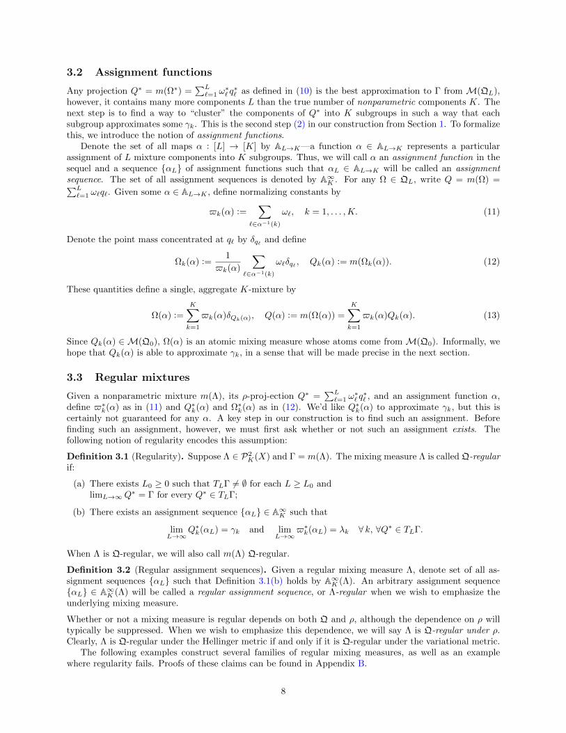
Overview Before outlining the formal details, we present an intuitive geometric picture of our approachin Figure 1. This same example is developed in more detail in the experiments (see Section 6, Figure 4iv).At a high-level, our strategy for identifying the mixture distribution (1) is the following:

(1) Approximate Γ with an overfitted mixture of L K Gaussians (Figure 1b);

(2) Cluster these L Gaussian components into K groups such that each group roughly approximates someγk (Figure 1c);

(3) Use this clustering to define a new mixing measure (Figure 1d);

(4) Show that this new mixing measure converges to the true mixing measure Λ as L→∞.

Of course, this construction is not guaranteed to succeed for arbitrary mixing measures Λ, which will beillustrated by the examples in Section 2.2. This is a surprisingly subtle problem and requires careful consid-eration of the various spaces involved. Thus, a key aspect of our analysis will be to provide assumptions thatensure the success of this construction. Intuitively, it should be clear that as long as the γk are well-separated,the corresponding mixture approximation will consist of Gaussian components that are also well-separated.Unfortunately, this is not quite enough to imply identifiability, as illustrated by Example 5. This highlightssome of the subtleties inherent in this construction. Furthermore, although we have used mixtures of Gaus-sians to approximate Γ in this example, our main results will apply to any properly chosen family of basemeasures.

2 Preliminaries

Our approach is general, built on the theory of abstract measures on metric spaces [54]. In this section weintroduce this abstract setting, outline our notation, and discuss the general problem of identifiability inmixture models. For a more thorough introduction to the general topic of mixture models in statistics, seeLindsay [48], Ritter [57], Titterington et al. [72].

2.1 Nonparametric mixture models

Let (X, d) be a metric space and (P(X), ρ) denote the space of regular Borel probability measures on Xwith finite rth moments (r ≥ 1) metrized by a metric ρ. Common choices for ρ include the Hellinger andvariational metrics, however, our results will apply to any metric on P(X). Define P2(X) = P(P(X)), thespace of (infinite) mixing measures over P(X). In this paper, we study finite mixture models, i.e. mixtureswith a finite number of atoms. To this end, define for s ∈ 1, 2, . . .

P2s (X) := Λ ∈ P2(X) : | supp(Λ)| ≤ s, P2

0 (X) :=

∞⋃s=1

P2s (X).

3

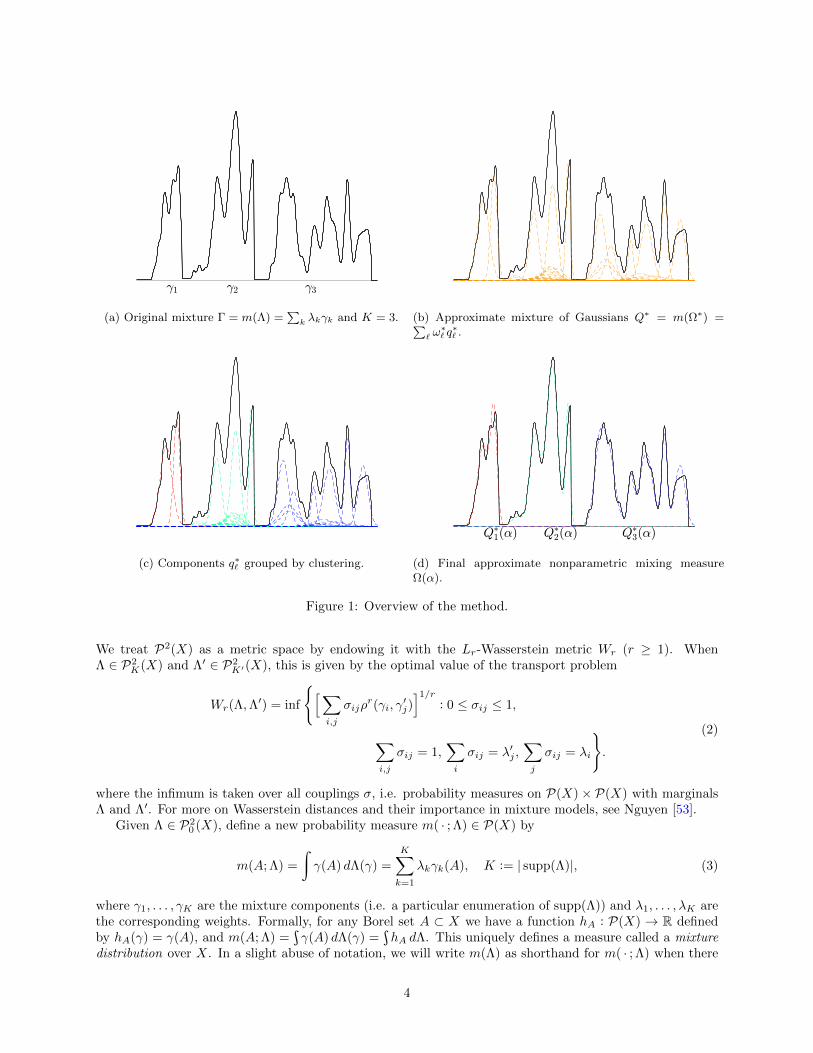
(a) Original mixture Γ = m(Λ) =∑

k λkγk and K = 3. (b) Approximate mixture of Gaussians Q∗ = m(Ω∗) =∑` ω

∗` q

∗` .

(c) Components q∗` grouped by clustering. (d) Final approximate nonparametric mixing measureΩ(α).

Figure 1: Overview of the method.

We treat P2(X) as a metric space by endowing it with the Lr-Wasserstein metric Wr (r ≥ 1). WhenΛ ∈ P2

K(X) and Λ′ ∈ P2K′(X), this is given by the optimal value of the transport problem

Wr(Λ,Λ′) = inf

[∑i,j

σijρr(γi, γ

′j)]1/r

: 0 ≤ σij ≤ 1,

∑i,j

σij = 1,∑i

σij = λ′j ,∑j

σij = λi

.

(2)

where the infimum is taken over all couplings σ, i.e. probability measures on P(X)× P(X) with marginalsΛ and Λ′. For more on Wasserstein distances and their importance in mixture models, see Nguyen [53].

Given Λ ∈ P20 (X), define a new probability measure m( · ; Λ) ∈ P(X) by

m(A; Λ) =

ż

γ(A) dΛ(γ) =

K∑k=1

λkγk(A), K := | supp(Λ)|, (3)

where γ1, . . . , γK are the mixture components (i.e. a particular enumeration of supp(Λ)) and λ1, . . . , λK arethe corresponding weights. Formally, for any Borel set A ⊂ X we have a function hA : P(X) → R definedby hA(γ) = γ(A), and m(A; Λ) =

ş

γ(A) dΛ(γ) =ş

hA dΛ. This uniquely defines a measure called a mixturedistribution over X. In a slight abuse of notation, we will write m(Λ) as shorthand for m( · ; Λ) when there

4

is no confusion between the arguments. An element γk of supp(Λ) is called a mixture component. Given aBorel set L ⊂ P2(X), define in analogy with P2

s (X) the subsets of finite mixtures by

Ls = L ∩ P2s (X) (4)

and

M(L) := m(Λ) : Λ ∈ L, (5)

i.e. the family of mixture distributions over X induced by L, which can be regarded as a formal representationof a statistical mixture model.

Remark 2.1. This abstract presentation of mixture models is needed for two reasons: (i) To emphasize thatΛ is the statistical parameter of interest, in contrast to the usual parametrization in terms of atoms andweights; and (ii) To emphasize that our approach works for general measures on metric spaces. This willhave benefits in the sequel, albeit at the cost of some extra abstraction here at the onset. For the most part,we will work with finite mixtures, i.e. P2

0 (X), a space which should be contrasted with the more complexspace of infinite measures P2(X), although some of the examples and proofs will invoke infinite mixtures.

Remark 2.2. As a convention, we will use upper case letters for mixture distributions (e.g. Γ, Q) and mixingmeasures (e.g. Λ, Ω), and lower case letters for mixture components (e.g. γk, qk) and weights (e.g. λk, ωk).

We conclude this subsection with some examples.

Example 1 (Parametric mixtures). Let Q = qθ : θ ∈ Θ be a family of measures parametrized by θ.Then any mixing measure whose support is contained in Q defines a parametric mixture distribution. Forexample, let G ⊂ P2(Rp) denote the subset of mixing measures whose support is contained in the family ofp-dimensional Gaussian measures. ThenM(G) is the family of Gaussian mixtures, andM(G0) is the familyof finite Gaussian mixtures. It is well-known that M(G0) is identifiable [68, 69]. Other examples includecertain exponential family mixtures [8] and translation families [68] (i.e. qθ(A) = µ(A− θ) for some knownmeasure µ ∈ P(Rd)).

Example 2 (Sub-Gaussian mixtures). Let K be the collection sub-Gaussian measures on R, i.e.

K = γ ∈ P(R) : γ(x : |x| > t) ≤ e1−t2/c2 for some c > 0 and all t > 0,

and K ⊂ P2(R) be the subset of mixing measures whose support is a subset of K. Then M(K) is thefamily of sub-Gaussian mixture models and M(K0) is the family of finite sub-Gaussian mixtures. This is anonparametric mixture model, since the base measures K do not belong to a parametric family. Extensionsto sub-Gaussian measures on Rp are natural.

Our definition of mixtures over subsets of mixing measures—as opposed to over families of componentdistributions—makes it easy to encode additional constraints, as in the following example.

Example 3 (Constrained mixtures). Continuing the previous example, suppose we wish to impose additionalconstraints on the family of mixture distributions. For example, we might be interested in Gaussian mixtureswhose means are contained within some set A ⊂ Rp and whose covariance matrices are contained withinanother set V ⊂ PD(p), where PD(p) is the set of p × p positive-definite matrices. Define G(A, V ) :=N (a, v) : a ∈ A, v ∈ V and

G(A, V ) := Λ ∈ P2(X) : supp(Λ) ⊂ G(A, V ). (6)

Then M(G(A, V )) is the desired family of mixture models. A special case of interest is V = v for somefixed v ∈ PD(p), which we denote by G(A, v), also known as a convolutional (Gaussian) mixture model.Finite mixtures from these families are denoted by M(G0(A, V )) and M(G0(A, v)).

Example 4 (Mixture of regressions). Suppose P(Y |Z) =ş

γ(Z) dΛ(γ) is a mixture model depending onsome covariates Z. We assume here that (Z, Y ) ∈W×X where (W,dW ) and (X, dX) are metric spaces. This

5

a1 a2 a3

a1 a2 a3 a1 a2 a3 a1 a2 a3

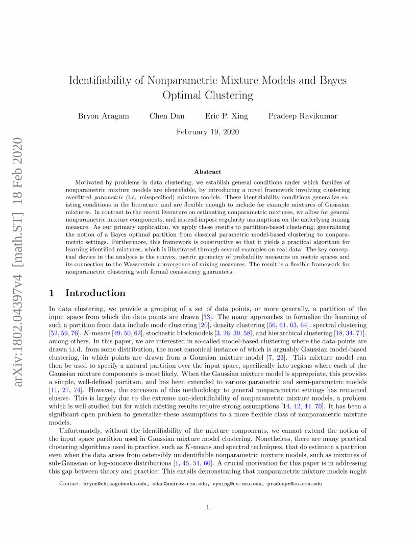
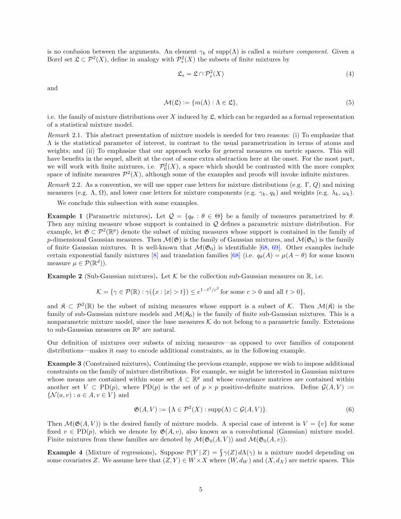
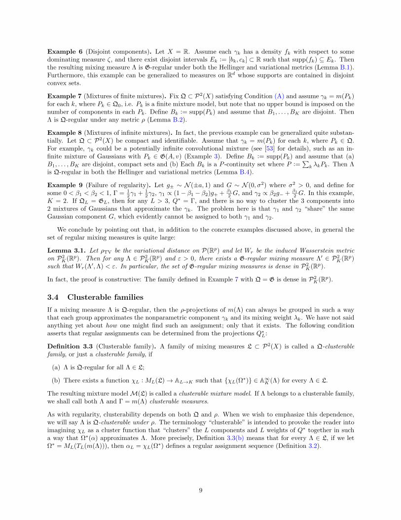
Figure 2: (top) Mixture of three Gaussians. (bottom) Different representations of a mixture of Gaussians asa mixture of two sub-Gaussians. Different fill patterns and colours represent different assignments of mixturecomponents.

is a nonparametric extension of the usual mixed linear regression model. To recover the mixed regressionmodel, assume Λ has at most K atoms and γk(Z) ∼ N (〈θk, Z〉, ω2

k), so that

P(Y |Z) =

ż

γ(Z) dΛ(γ) =

K∑k=1

λkN (〈θk, Z〉, ω2k).

By further allowing the mixing measure Λ = Λ(Z) to depend on the covariates, we obtain the nonparametricgeneralization of a mixture of experts model [15, 41, 43].

2.2 Identifiability in mixture models

A mixture model M(L) is identifiable if the map m : L→M(L) that sends Λ 7→ m(Λ) is injective. For anoverview of this problem, see Hunter et al. [42] and Allman et al. [4]. The main purpose of this section is tohighlight some of the known subtleties in identifying nonparametric mixture models.

Unsurprisingly, whether or not a specific mixture m(Λ) is identified depends on the choice of L. If weallow L to be all of P2(X), then it is easy to see that M(L) is not identifiable, and this continues to betrue even if the number of components K is known in advance (i.e. L = P2

K(X)). Indeed, for any partitionAkKk=1 of X and any Borel set B ⊂ X, we can write

Γ(B) =

K∑k=1

Γ(Ak)︸ ︷︷ ︸λk

· Γ(B ∩Ak)

Γ(Ak)︸ ︷︷ ︸γk

=

K∑k=1

λkγk(B), (7)

and thus there cannot be a unique decomposition of the measure Γ into the sum (1). Although this exampleallows for arbitrary, pathological decompositions of Γ into conditional measures, the following concreteexample shows that solving the nonidentifiability issue is more complicated than simply avoiding certainpathological partitions of the input space.

Example 5 (Sub-Gaussian mixtures are not identifiable). Consider the mixture of three Gaussians m(Λ) inFigure 2. We can write m(Λ) as a mixture in four ways: In the top panel, m(Λ) is represented uniquely asa mixture of three Gaussians. If we allow sub-Gaussian components, however, then the bottom panel showsthree equally valid representations of m(Λ) as a mixture of two sub-Gaussians. Indeed, even if we assume thenumber of components K is known and the component means are well-separated, m(Λ) is non-identifiableas a mixture of sub-Gaussians: Just take K = 2, |a1 − a2| > 0 and move a3 arbitrarily far to the right.

Much of the existing literature makes assumptions on the structure of the allowed γk, which is evidentlyequivalent to restricting the supports of the mixing measures in L (e.g. Example 1). Our focus, by contrast,will be to allow the components to take on essentially any shape while imposing regularity assumptions onthe mixing measures Λ ∈ L. In this sense, we shift the focus from the properties of the “local” mixturecomponents to the “global” properties of the mixture itself.

6

3 Regularity and clusterability

Fix an integer K and let L ⊂ P2K(X) be a family of mixing measures. In particular, we assume that K—the

number of nonparametric mixtures—is known; in Section 7 we discuss the case where K is unknown. Inthis section we study conditions that guarantee the injectivity of the embedding m : L →M(L) using theprocedure described in Section 1. Throughout this section, it will be helpful to keep Figure 1 in mind forintuition.

3.1 Projections

Let QL∞L=1 be an indexed collection of families of mixing measures that satisfies the following:

(A1) QL ⊂ P2L(X) for each L;

(A2) QL is monotonic, i.e. QL ⊂ QL+1;

(A3) M(QL) is identifiable for each L.

The purpose of QL is to approximate Γ with a sequence of mixture distributions of increasing complexity,as quantified by the maximum number of atoms L, which will be taken to be much larger than K. Althoughour results apply to generic collections satisfying Conditions (A1)-(A3), in the sequel we will consider thecollection induced by a single subset Q ⊂ P2(X) and defined by QL = Q ∩ P2

L(X) (cf. (4)). We make thefollowing assumption on Q:

(A) The collection QL∞L=1 defined by QL = Q∩P2L(X) satisfies Condition (A3) for the family Q ⊂ P2(X).

If Q satisfies Condition (A), then QL automatically satisfies Conditions (A1)-(A3). Examples of fami-lies that satisfy Condition (A) include exponential family mixture models under certain conditions [8], forexample Gaussian or Gamma mixtures [69].

Unless otherwise mentioned, we will assume Q satisfies Condition (A), with QL as defined therein. Definethe usual ρ-projection by

TLΓ =Q ∈M(QL) : ρ(Q,Γ) ≤ ρ(P,Γ) ∀P ∈M(QL)

. (8)

As long as Q is compact, the projection TLΓ is nonempty. Furthermore, Condition (A3) implies that thereexists a well-defined map ML :M(QL)→ QL that sends a mixture distribution to its mixing measure. Withsome abuse of notation, we will write MLΓ for ML(TLΓ), i.e.

MLΓ =

Ω ∈ QL : m(Ω) ∈ TLΓ. (9)

Thus for any Q∗ ∈ TLΓ, we can unambiguously define

Q∗ =

L∑`=1

ω∗` q∗` = m(Ω∗) and Ω∗ = ML(Q∗). (10)

An example of the measure Q∗ and its mixing measure Ω∗ are depicted in Figure 1b.

Remark 3.1. We do not assume that TLΓ is unique, i.e. there may be more than one projection. This isbecause M(QL) is a nonconvex set. We present our results in this setting, however, it may be simpler on afirst reading to consider the special case where the projection is unique, i.e. TLΓ = Q∗ for each L. In thiscase, many of the definitions simplify: Consider for example Definition 3.1 and (18) in the sequel.

Remark 3.2. The number of overfitted mixture components L will play an important but largely unheraldedrole in the sequel. For the most part, we will suppress the dependence of various quantities (e.g. Q∗, Ω∗)on L for notational simplicity. In Section 4.2, we discuss how to choose L given the sample size n; seeCorollary 4.4.

7

3.2 Assignment functions

Any projection Q∗ = m(Ω∗) =∑L`=1 ω

∗` q∗` as defined in (10) is the best approximation to Γ from M(QL),

however, it contains many more components L than the true number of nonparametric components K. Thenext step is to find a way to “cluster” the components of Q∗ into K subgroups in such a way that eachsubgroup approximates some γk. This is the second step (2) in our construction from Section 1. To formalizethis, we introduce the notion of assignment functions.

Denote the set of all maps α : [L] → [K] by AL→K—a function α ∈ AL→K represents a particularassignment of L mixture components into K subgroups. Thus, we will call α an assignment function in thesequel and a sequence αL of assignment functions such that αL ∈ AL→K will be called an assignmentsequence. The set of all assignment sequences is denoted by A∞K . For any Ω ∈ QL, write Q = m(Ω) =∑L`=1 ω`q`. Given some α ∈ AL→K , define normalizing constants by

$k(α) :=∑

`∈α−1(k)

ω`, k = 1, . . . ,K. (11)

Denote the point mass concentrated at q` by δq` and define

Ωk(α) :=1

$k(α)

∑`∈α−1(k)

ω`δq` , Qk(α) := m(Ωk(α)). (12)

These quantities define a single, aggregate K-mixture by

Ω(α) :=

K∑k=1

$k(α)δQk(α), Q(α) := m(Ω(α)) =

K∑k=1

$k(α)Qk(α). (13)

Since Qk(α) ∈ M(Q0), Ω(α) is an atomic mixing measure whose atoms come from M(Q0). Informally, wehope that Qk(α) is able to approximate γk, in a sense that will be made precise in the next section.

3.3 Regular mixtures

Given a nonparametric mixture m(Λ), its ρ-proj-ection Q∗ =∑L`=1 ω

∗` q∗` , and an assignment function α,

define $∗k(α) as in (11) and Q∗k(α) and Ω∗k(α) as in (12). We’d like Q∗k(α) to approximate γk, but this iscertainly not guaranteed for any α. A key step in our construction is to find such an assignment. Beforefinding such an assignment, however, we must first ask whether or not such an assignment exists. Thefollowing notion of regularity encodes this assumption:

Definition 3.1 (Regularity). Suppose Λ ∈ P2K(X) and Γ = m(Λ). The mixing measure Λ is called Q-regular

if:

(a) There exists L0 ≥ 0 such that TLΓ 6= ∅ for each L ≥ L0 andlimL→∞Q∗ = Γ for every Q∗ ∈ TLΓ;

(b) There exists an assignment sequence αL ∈ A∞K such that

limL→∞

Q∗k(αL) = γk and limL→∞

$∗k(αL) = λk ∀ k, ∀Q∗ ∈ TLΓ.

When Λ is Q-regular, we will also call m(Λ) Q-regular.

Definition 3.2 (Regular assignment sequences). Given a regular mixing measure Λ, denote set of all as-signment sequences αL such that Definition 3.1(b) holds by A∞K (Λ). An arbitrary assignment sequenceαL ∈ A∞K (Λ) will be called a regular assignment sequence, or Λ-regular when we wish to emphasize theunderlying mixing measure.

Whether or not a mixing measure is regular depends on both Q and ρ, although the dependence on ρ willtypically be suppressed. When we wish to emphasize this dependence, we will say Λ is Q-regular under ρ.Clearly, Λ is Q-regular under the Hellinger metric if and only if it is Q-regular under the variational metric.

The following examples construct several families of regular mixing measures, as well as an examplewhere regularity fails. Proofs of these claims can be found in Appendix B.

8

Example 6 (Disjoint components). Let X = R. Assume each γk has a density fk with respect to somedominating measure ζ, and there exist disjoint intervals Ek := [bk, ck] ⊂ R such that supp(fk) ⊆ Ek. Thenthe resulting mixing measure Λ is G-regular under both the Hellinger and variational metrics (Lemma B.1).Furthermore, this example can be generalized to measures on Rd whose supports are contained in disjointconvex sets.

Example 7 (Mixtures of finite mixtures). Fix Q ⊂ P2(X) satisfying Condition (A) and assume γk = m(Pk)for each k, where Pk ∈ Q0, i.e. Pk is a finite mixture model, but note that no upper bound is imposed on thenumber of components in each Pk. Define Bk := supp(Pk) and assume that B1, . . . , BK are disjoint. ThenΛ is Q-regular under any metric ρ (Lemma B.2).

Example 8 (Mixtures of infinite mixtures). In fact, the previous example can be generalized quite substan-tially. Let Q ⊂ P2(X) be compact and identifiable. Assume that γk = m(Pk) for each k, where Pk ∈ Q.For example, γk could be a potentially infinite convolutional mixture (see [53] for details), such as an in-finite mixture of Gaussians with Pk ∈ G(A, v) (Example 3). Define Bk := supp(Pk) and assume that (a)B1, . . . , BK are disjoint, compact sets and (b) Each Bk is a P -continuity set where P :=

∑k λkPk. Then Λ

is Q-regular in both the Hellinger and variational metrics (Lemma B.4).

Example 9 (Failure of regularity). Let g± ∼ N (±a, 1) and G ∼ N (0, σ2) where σ2 > 0, and define forsome 0 < β1 < β2 < 1, Γ = 1

2γ1 + 12γ2, γ1 ∝ (1− β1 − β2)g+ + β1

2 G, and γ2 ∝ β2g− + β1

2 G. In this example,K = 2. If QL = GL, then for any L > 3, Q∗ = Γ, and there is no way to cluster the 3 components into2 mixtures of Gaussians that approximate the γk. The problem here is that γ1 and γ2 “share” the sameGaussian component G, which evidently cannot be assigned to both γ1 and γ2.

We conclude by pointing out that, in addition to the concrete examples discussed above, in general theset of regular mixing measures is quite large:

Lemma 3.1. Let ρTV be the variational distance on P(Rp) and let Wr be the induced Wasserstein metricon P2

K(Rp). Then for any Λ ∈ P2K(Rp) and ε > 0, there exists a G-regular mixing measure Λ′ ∈ P2

K(Rp)such that Wr(Λ

′,Λ) < ε. In particular, the set of G-regular mixing measures is dense in P2K(Rp).

In fact, the proof is constructive: The family defined in Example 7 with Q = G is dense in P2K(Rp).

3.4 Clusterable families

If a mixing measure Λ is Q-regular, then the ρ-projections of m(Λ) can always be grouped in such a waythat each group approximates the nonparametric component γk and its mixing weight λk. We have not saidanything yet about how one might find such an assignment; only that it exists. The following conditionasserts that regular assignments can be determined from the projections Q∗L:

Definition 3.3 (Clusterable family). A family of mixing measures L ⊂ P2(X) is called a Q-clusterablefamily, or just a clusterable family, if

(a) Λ is Q-regular for all Λ ∈ L;

(b) There exists a function χL : ML(L)→ AL→K such that χL(Ω∗) ∈ A∞K (Λ) for every Λ ∈ L.

The resulting mixture modelM(L) is called a clusterable mixture model. If Λ belongs to a clusterable family,we shall call both Λ and Γ = m(Λ) clusterable measures.

As with regularity, clusterability depends on both Q and ρ. When we wish to emphasize this dependence,we will say Λ is Q-clusterable under ρ. The terminology “clusterable” is intended to provoke the reader intoimagining χL as a cluster function that “clusters” the L components and L weights of Q∗ together in sucha way that Ω∗(α) approximates Λ. More precisely, Definition 3.3(b) means that for every Λ ∈ L, if we letΩ∗ = ML(TL(m(Λ))), then αL = χL(Ω∗) defines a regular assignment sequence (Definition 3.2).

9

3.5 Separation and clusterability

In this section, we construct an explicit cluster function χL via single-linkage clustering.Given Ω ∈ QL with atoms q`, define the ρ-diameter of Ω by

∆(Ω) := supρ(q, q′) : q, q′ ∈ conv(supp(Ω))

where conv( · ) is the convex hull in P(X). Recalling (13), define for any α ∈ AL→K

η(Ω(α)) := supk

∆(Ωk(α)) + supkρ(γk, Qk(α)). (14)

We will be interested in the special case Ω = Ω∗: ∆(Ω∗k(α)) quantifies how “compact” the mixture componentQ∗k(α) is and η(Ω∗(α)) is a measure of separation between the mixture components γk. Finally, define theρ-distance matrix by

D(Ω) = (ρ(qi, qj))Li,j=1. (15)

Our goal is to show that if the atoms of Λ are sufficiently well-separated, then the cluster assignment αcan be reconstructed by clustering the distance matrix D∗ = D(Ω∗) = (ρ(q∗i , q

∗j ))Li,j=1 (hence the choice of

terminology clusterable). More precisely, we make the following definition:

Definition 3.4 (Separation). A mixing measure Λ ∈ P20 (X) is called δ-separated if infi 6=j ρ(γi, γj) > δ for

some δ > 0.

It turns out that separation of the order η(Ω∗(α)) (cf. (14)) is sufficient to define a cluster function:

Proposition 3.2. Let Λ ∈ P2K(X). Let Q∗ ∈ TLΓ be a ρ-projection of Γ for some L ≥ K. Then for any

α ∈ AL→K such that Λ is 4η(Ω∗(α))-separated,

α(i) = α(j) ⇐⇒ ρ(q∗i , q∗j ) ≤ η(Ω∗(α)), (16)

α(i) 6= α(j) ⇐⇒ ρ(q∗i , q∗j ) ≥ 2η(Ω∗(α)). (17)

Moreover, α can be recovered by single-linkage clustering on D∗.

Thus, the assignment α can be recovered by single-linkage clustering of D∗ without knowing the optimalthreshold η(Ω∗(α)).

Now suppose Λ is a regular mixing measure and let αL ∈ A∞K (Λ). Define

η(Λ) := lim supL→∞

supΩ∗∈MLΓ

supαL∈A∞K (Λ)

η(Ω∗(αL)). (18)

As a consequence of regularity, the second term in (14) tends to zero as L → ∞, so that η(Λ) canbe interpreted as a measure of the asymptotic diameter of the approximating mixtures Q∗k(αL). Forexample, when the ρ-projection Q∗ is unique (Remark 3.1) the definition in (18) simplifies to η(Λ) =lim supL supk ∆(Ω∗k(αL)). The following corollary, which is an immediate consequence of Proposition 3.2,shows that control over η(Λ) is sufficient for L to be clusterable:

Corollary 3.3. Suppose L ⊂ P2K(X) is a family of regular mixing measures such that for every Λ ∈ L there

exists ξ > 0 such that Λ is (4 + ξ)η(Λ)-separated. Then L is clusterable.

Thus, we have a practical separation condition under which a regular mixture model becomes identifiable:

infi6=j

ρ(γi, γj) > (4 + ξ)η(Λ). (19)

In the limit L → ∞, the nonparametric components γk must be separated by a gap proportional to theρ-diameters of the approximating mixtures Q∗k(αL). This highlights the issue in Example 5—although themeans can be arbitrarily separated, as we increase the separation, the diameter of the components continuesto increase as well. Thus, the γk cannot be chosen in a haphazard way (see also Example 9). Crucially,however, we make no assumptions on the shape of the mixture components.

10

Example 10 (Example of separation). Take X = R and let Q = G(A, v) be a family of convolutionalmixtures of Gaussians (Example 3). In Example 8, we claimed that as long as the Pk have disjoint supports,this family is G(A, v)-regular. To determine when a mixing measure Λ is G(A, v)-clusterable, it sufficesto check (19). For this, we bound the ρ-diameters supk ∆(Ω∗k(αL)) for large L. If q` ∼ N (a`, v

2) andq`′ ∼ N (a`′ , v

2) are both in supp(Pk), then it is easy to check that as long as

|a` − a`′ | ≤√

8v2 log(1 + ρ∗

4−ρ∗

), ρ∗ := inf

i 6=jρ(γi, γj),

the separation condition (19) holds.

The separation condition (19) is quite weak, but no attempt has been made here to optimize this lowerbound. For example, a minor tweak to the proof can reduce the constant of 4 to any constant b > 2. Althoughwe expect that a more careful analysis can weaken this condition, our main focus here is to present the mainidea behind identifiability and its connection to clusterability and separation, so we save such optimizationsfor future work. Further, although Proposition 3.2 justifies the use of single-linkage clustering in order togroup the components q∗` , one can easily imagine using other clustering schemes. Indeed, since the distancematrix D∗ is always well-defined, we could have applied other clustering algorithms such as complete-linkagehierarchical clustering, K-means, or spectral clustering to D∗ to define an assignment sequence αL. Anycondition on D∗ that ensures a clustering algorithm will correctly reconstruct a regular assignment sequencethen yields an identification condition in the spirit of Proposition 3.2. For example, if the means of theoverfitted components q∗` are always well-separated, then simple algorithms such as K-means could sufficeto identify a regular assignment sequence. This highlights the advantage of our abstract viewpoint, in whichthe specific forms of both the assignment sequence αL and the cluster functions χL are left unspecified.

4 Identifiability and estimation

We now turn our attention to the problem of identifying and learning a mixing measure Λ from data.

4.1 Identifiability of nonparametric mixtures

According to the next theorem, clusterability is sufficient to identify a nonparametric mixture model.

Theorem 4.1. If L is a Q-clusterable family then the mixture model M(L) is identifiable.

As illustrated by the cautionary tales from Examples 5 and 9, identification in nonparametric mixtures is asubtle problem, and this theorem thus provides a powerful general condition for identifiability in nonpara-metric problems.

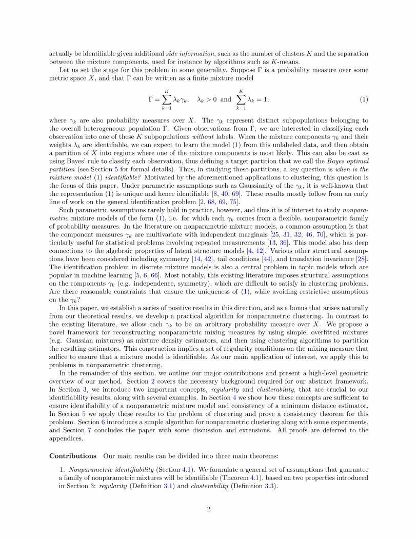
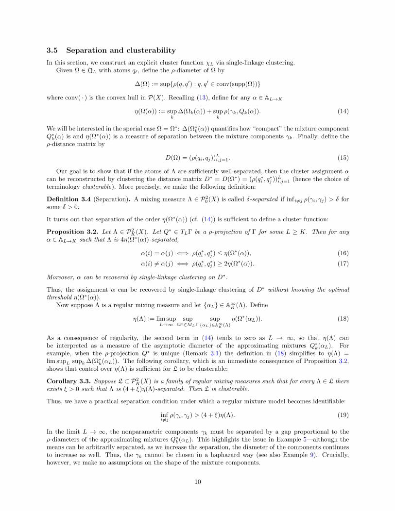
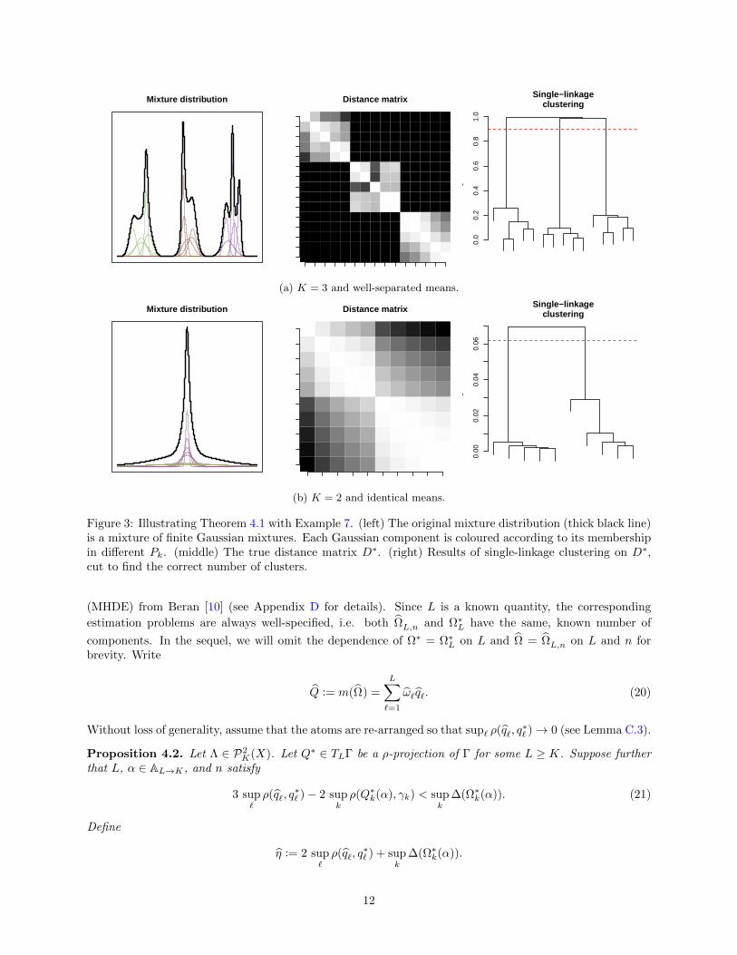
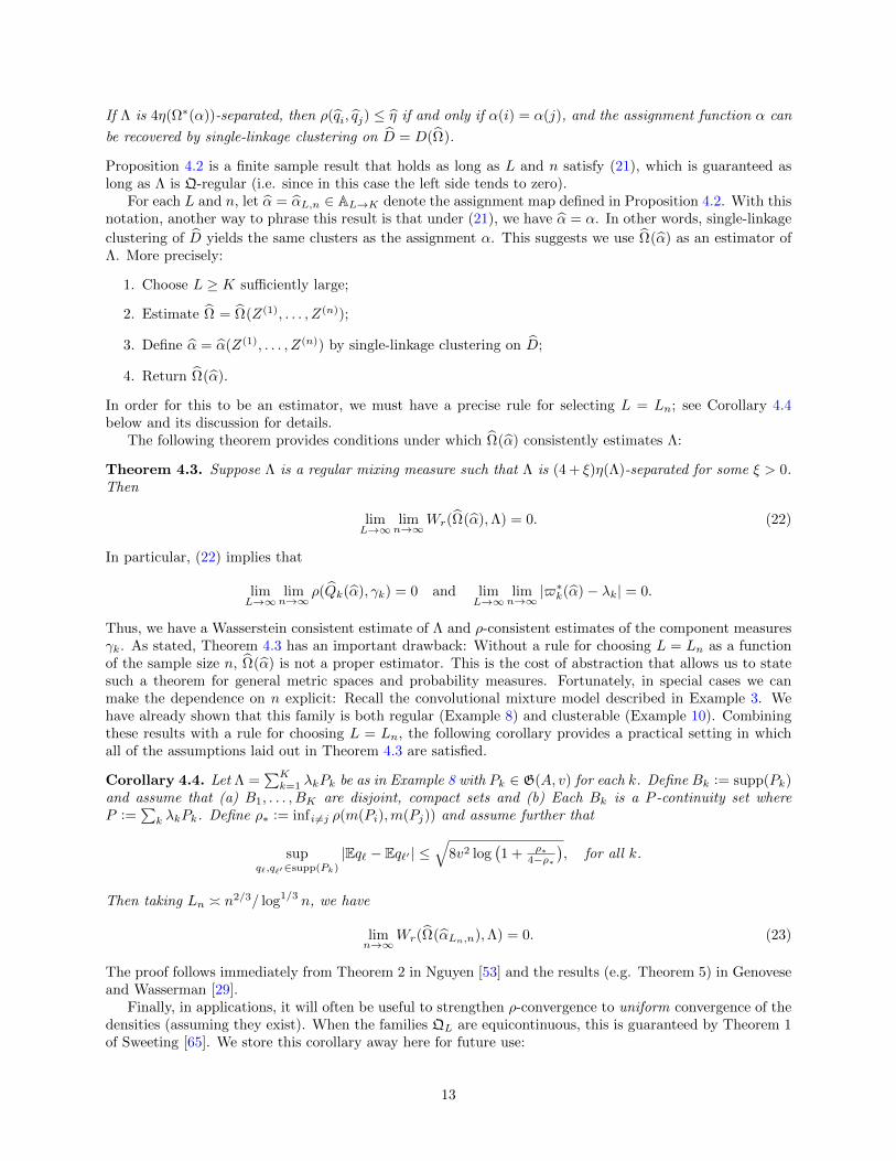
Two examples of Theorem 4.1 are illustrated in Figure 3. When the means are well-separated as inFigure 3a, it is easy to see how single-linkage clustering is able to discover a correct assignment. Sinceρ-separation is a weaker criterion than mean separation, however, Theorem 4.1 does not require that themixture distributions in M(L) have components with well-separated means. In fact, each γk could haveidentical means (but different variances) and still be well-separated. This is illustrated in Figure 3b. Thissuggests that identifiability in mixture models is more general than what is needed in typical clusteringapplications, where a model such as Figure 3b would not be considered to have two distinct clusters. Thesubtlety here lies in interpreting clustering in P(X) (i.e. of the q∗` ) vs. clustering in X (i.e. of samplesZ(i) ∼ Γ), the latter of which is the interpretation used in data clustering.

4.2 Estimation of clusterable mixtures

We now discuss how to estimate Λ from data Z(1), . . . , Z(n) iid∼ Γ. Throughout this section, we assume thatΩ∗ = Ω∗L ∈MLΓ is arbitrary.

For each L ≥ K, let ΩL,n = ΩL(Z(1), . . . , Z(n)) be a Wr-consistent estimator of Ω∗L, where we have written

ΩL,n and Ω∗L to emphasize the dependence on L and n. That is, ΩL,n is a sequence of estimators and for

each L, limn→∞Wr(ΩL,n,Ω∗L) = 0. For example, ΩL,n could be the minimum Hellinger distance estimator

11

Mixture distribution Distance matrix

0.0

0.2

0.4

0.6

0.8

1.0

Single−linkageclustering

Hei

ght

(a) K = 3 and well-separated means.

Mixture distribution Distance matrix

0.00

0.02

0.04

0.06

Single−linkageclustering

Hei

ght

(b) K = 2 and identical means.

Figure 3: Illustrating Theorem 4.1 with Example 7. (left) The original mixture distribution (thick black line)is a mixture of finite Gaussian mixtures. Each Gaussian component is coloured according to its membershipin different Pk. (middle) The true distance matrix D∗. (right) Results of single-linkage clustering on D∗,cut to find the correct number of clusters.

(MHDE) from Beran [10] (see Appendix D for details). Since L is a known quantity, the corresponding

estimation problems are always well-specified, i.e. both ΩL,n and Ω∗L have the same, known number of

components. In the sequel, we will omit the dependence of Ω∗ = Ω∗L on L and Ω = ΩL,n on L and n forbrevity. Write

Q := m(Ω) =

L∑`=1

ω`q`. (20)

Without loss of generality, assume that the atoms are re-arranged so that sup` ρ(q`, q∗` )→ 0 (see Lemma C.3).

Proposition 4.2. Let Λ ∈ P2K(X). Let Q∗ ∈ TLΓ be a ρ-projection of Γ for some L ≥ K. Suppose further

that L, α ∈ AL→K , and n satisfy

3 sup`ρ(q`, q

∗` )− 2 sup

kρ(Q∗k(α), γk) < sup

k∆(Ω∗k(α)). (21)

Define

η := 2 sup`ρ(q`, q

∗` ) + sup

k∆(Ω∗k(α)).

12

If Λ is 4η(Ω∗(α))-separated, then ρ(qi, qj) ≤ η if and only if α(i) = α(j), and the assignment function α can

be recovered by single-linkage clustering on D = D(Ω).

Proposition 4.2 is a finite sample result that holds as long as L and n satisfy (21), which is guaranteed aslong as Λ is Q-regular (i.e. since in this case the left side tends to zero).

For each L and n, let α = αL,n ∈ AL→K denote the assignment map defined in Proposition 4.2. With thisnotation, another way to phrase this result is that under (21), we have α = α. In other words, single-linkage

clustering of D yields the same clusters as the assignment α. This suggests we use Ω(α) as an estimator ofΛ. More precisely:

1. Choose L ≥ K sufficiently large;

2. Estimate Ω = Ω(Z(1), . . . , Z(n));

3. Define α = α(Z(1), . . . , Z(n)) by single-linkage clustering on D;

4. Return Ω(α).

In order for this to be an estimator, we must have a precise rule for selecting L = Ln; see Corollary 4.4below and its discussion for details.

The following theorem provides conditions under which Ω(α) consistently estimates Λ:

Theorem 4.3. Suppose Λ is a regular mixing measure such that Λ is (4 + ξ)η(Λ)-separated for some ξ > 0.Then

limL→∞

limn→∞

Wr(Ω(α),Λ) = 0. (22)

In particular, (22) implies that

limL→∞

limn→∞

ρ(Qk(α), γk) = 0 and limL→∞

limn→∞

|$∗k(α)− λk| = 0.

Thus, we have a Wasserstein consistent estimate of Λ and ρ-consistent estimates of the component measuresγk. As stated, Theorem 4.3 has an important drawback: Without a rule for choosing L = Ln as a functionof the sample size n, Ω(α) is not a proper estimator. This is the cost of abstraction that allows us to statesuch a theorem for general metric spaces and probability measures. Fortunately, in special cases we canmake the dependence on n explicit: Recall the convolutional mixture model described in Example 3. Wehave already shown that this family is both regular (Example 8) and clusterable (Example 10). Combiningthese results with a rule for choosing L = Ln, the following corollary provides a practical setting in whichall of the assumptions laid out in Theorem 4.3 are satisfied.

Corollary 4.4. Let Λ =∑Kk=1 λkPk be as in Example 8 with Pk ∈ G(A, v) for each k. Define Bk := supp(Pk)

and assume that (a) B1, . . . , BK are disjoint, compact sets and (b) Each Bk is a P -continuity set whereP :=

∑k λkPk. Define ρ∗ := infi 6=j ρ(m(Pi),m(Pj)) and assume further that

supq`,q`′∈supp(Pk)

|Eq` − Eq`′ | ≤√

8v2 log(1 + ρ∗

4−ρ∗

), for all k.

Then taking Ln n2/3/ log1/3 n, we have

limn→∞

Wr(Ω(αLn,n),Λ) = 0. (23)

The proof follows immediately from Theorem 2 in Nguyen [53] and the results (e.g. Theorem 5) in Genoveseand Wasserman [29].

Finally, in applications, it will often be useful to strengthen ρ-convergence to uniform convergence of thedensities (assuming they exist). When the families QL are equicontinuous, this is guaranteed by Theorem 1of Sweeting [65]. We store this corollary away here for future use:

13

Corollary 4.5. Let Gk(α) be the density of Qk(α) and fk be the density of γk. If the families QL are

equicontinuous for all L and Qk(α) converges weakly to γk, then limL→∞ limn→∞ Gk(α) = fk, where thelimits are understood both pointwise and uniformly over compact subsets of X.

The assumption that Qk(α) converges weakly to γk restricts the choice of ρ, although it allows most reason-able metrics including Hellinger, variational, and Wasserstein, for example. Moreover, even weaker assump-tions than equicontinuity are possible [22].

5 Bayes optimal clustering

As an application of the theory developed in Sections 3 and 4, we extend model-based clustering [11, 27] tothe nonparametric setting. Given samples from Λ, we seek to partition these samples into K clusters. Moregenerally, Λ defines a partition of the input space X, which can be formalized as a function c : X → [K],where K is the number of partitions or “clusters”. First, let us recall the classical Gaussian mixture model(GMM): If f1(·; a1, v1), . . . , fK(·; aK , vK) is a collection of Gaussian density functions, then for any choice ofλk ≥ 0 such that

∑k λk = 1 the combination

F (z) =

K∑k=1

λkfk(z; ak, vk); z ∈ Rd (24)

is a GMM. The model (24) is of course equivalent to the integral (3) (see also Example 1), and the Gaussiandensities fk(z; ak, vk) can obviously be replaced with any family of parametric densities.

Intuitively, the density F has K distinct clusters given by the K Gaussian densities fk, defining what wecall the Bayes optimal partition over X into regions where each of the Gaussian components is most likely.It should be obvious that as long as a mixture model M(L) is identifiable, the Bayes optimal partition willbe well-defined and has a unique interpretation in terms of distinct clusters of the input space X. Thus, thetheory developed in the previous sections can be used to extend these ideas to the nonparametric setting.Since the clustering literature is full of examples of datasets that are not well-approximated by parametricmixtures [e.g. 52, 73], there is significant interest in such an extension. In the remainder of this section, wewill apply our framework to this problem. First, we discuss identifiability issues with the concept of a Bayesoptimal partition (Section 5.1). Then, we provide conditions under which a Bayes optimal partition can belearned from data (Section 5.2).

5.1 Bayes optimal partitions

Throughout the rest of this section, we assume that X is compact and all probability measures are absolutelycontinuous with respect to some base measure ζ, and hence have density functions. Assume Γ is fixed andwrite F = FΓ for the density of Γ and fk for the density of γk. Thus whenever Γ is a finite mixture we canwrite

F =

ż

fγ dΛ(γ) =

K∑k=1

λkfk. (25)

For any Λ ∈ P2K(X), define the usual Bayes classifier [e.g. 24]:

cΛ(x) := arg maxk∈[K]

λkfk(x). (26)

The classifier cΛ is only well-defined up to a permutation of the labels (i.e. any labeling of supp(Λ) definesan equivalent classifier). Furthermore, cΛ(x) not properly defined when λifi(x) = λjfj(x) for i 6= j. Toaccount for this, define an exceptional set

E0 :=⋃i 6=j

x ∈ X : λifi(x) = λjfj(x), (27)

14

In principle, E0 should be small—in fact it will typically have measure zero—hence we will be content topartition X0 = X − E0. Recall that a partition of a space X is a family of subsets Ak ⊂ X such thatAk ∩Ak′ = ∅ for all k 6= k′ and ∪kAk = X. We denote the space of all partitions of X by Π(X).

The following definition is standard [e.g. 17, 27]:

Definition 5.1 (Bayes optimal partition). Define an equivalence relation on X0 by declaring

x ∼ y ⇐⇒ cΛ(x) = cΛ(y). (28)

This relation induces a partition on X0 which we denote by πΛ or π(Λ). This partition is known as theBayes optimal partition.

Remark 5.1. Although the function cΛ is only unique up to a permutation, the partition defined by (28) isalways well-defined and independent of the permutation used to label the γk.

Given samples from the mixture distribution Γ = m(Λ), we wish to learn the Bayes optimal partitionπΛ. Unfortunately, there is—yet again—an identifiability issue: If there is more than one mixture measureΛ that represents Γ, the Bayes optimal partition is not well-defined.

Example 11 (Non-identifiability of Bayes optimal partition). In Example 5 and Figure 2, we have fourvalid representations of Γ as a mixture of sub-Gaussians. In all four cases, each representation leads to adifferent Bayes optimal partition, even though they each represent the same mixture distribution.

Clearly, if Λ is identifiable, then the Bayes optimal partition is automatically well-defined. Thus Theorem 4.1immediately implies the following:

Corollary 5.1. If M(L) is a clusterable mixture model, then there is a well-defined Bayes optimal partitionπΓ for any Γ ∈M(L).

In particular, whenever M(L) is clusterable it makes sense to write cΓ and πΓ instead of cΛ and πΛ,respectively. This provides a useful framework for discussing and analyzing partition-based clustering innonparametric settings. As discussed previously, a K-clustering of X is equivalent to a function that assignseach x ∈ X an integer from 1 to K, where K is the number of clusters. Clearly, up to the exceptional set E0,(26) is one such function. Thus, the Bayes optimal partition πΓ can be interpreted as a valid K-clustering.

5.2 Learning partitions from data

Write Γ = m(Λ) and assume that Λ is identifiable from Γ. Suppose we are given i.i.d. samples Z(1), . . . , Z(n) iid∼Γ and that we seek the Bayes optimal partition πΓ = πΛ. Our strategy will be the following:

1. Use a consistent estimator Ω to learn Ω∗ for some L K;

2. Theorem 4.3 guarantees that we can learn a cluster assignment α such that Ω(α) consistently estimatesΛ;

3. Use π(Ω(α)) to approximate πΛ = πΓ.

The hope, of course, is that π(Ω(α)) → πΓ. There are, however, complications: What do we mean by

convergence of partitions? Does π(Ω(α)) even converge, let alone converge to πΓ?

Instead of working directly with the partitions π(Ω(α)), we will work with the Bayes classifier (26). Write

g` and G for the densities of q` and Q, respectively, and

Gk(α) :=1

$k

∑`∈α−1(k)

ω`g`, $k(α) :=∑

`∈α−1(k)

ω`. (29)

Then Gk(α) is the density of Qk(α), where here and above we have suppressed the dependence on α. Nowdefine the estimated classifier (cf. (26))

c(x) := cΩ(α)(x) = arg maxk∈[K]

$k[Gk(α)](x). (30)

15

By considering classification functions as opposed to the partitions themselves, we may consider ordinaryconvergence of the function c to cΓ, which gives us a convenient notion of consistency for this problem.Furthermore, we can compare partitions by comparing the Bayes optimal equivalence classes Ak := c−1(k) =

x ∈ X : c(x) = k to the estimated equivalence classes AL,n,k := c−1(k) by controlling Ak4AL,n,k, whereA4B = (A−B)∪ (A−B) is the usual symmetric difference of two sets. Specifically, we’d like to show that

the difference Ak4AL,n,k is small. To this end, define a fattening of E0 by

E0(t) :=⋃i 6=j

x ∈ X : |λifi(x)− λjfj(x)| ≤ t, t > 0. (31)

Then of course E0 = E0(0). When the boundaries between classes are sharp, this set will be small, however,if two classes have substantial overlap, then E0(t) can be large even if t is small. In the latter case, theequivalence classes Ak (and hence the clusters) are less meaningful. The purpose of E0(t) is to account forsampling error in the estimated partition.

Theorem 5.2. Assume that limL→∞ limn→∞ Gk(α) = fk uniformly on X and υ is any measure on X.Then there exists a sequence tL,n → 0 such that c(x) = cΛ(x) for all x ∈ X − E0(tL,n) and

υ

(K⋃k=1

Ak4AL,n,k

)≤ υ(E0(tL,n))→ υ(E0). (32)

As in Corollary 4.4, under the same assumptions we may take L = Ln n2/3/ log1/3 n in Theorem 5.2 whenQ = G0(A, v).

The uniform convergence assumption in Theorem 5.2 may seem strong, however, recall Corollary 4.5,which guarantees uniform convergence whenever QL is equicontinuous. For example, recalling Examples 1and 3, it is straightforward to show the following:

Corollary 5.3. Suppose X ⊂ Rd, Q is a compact subset of G and υ is any measure on X. If Λ is Q-clusterable measure under the Hellinger or variational metric, then there exists a sequence tL,n → 0 suchthat c(x) = cΛ(x) for all x ∈ X − E0(tL,n) and

υ

(K⋃k=1

Ak4AL,n,k

)≤ υ(E0(tL,n))→ υ(E0). (33)

We can interpret Theorem 5.2 as follows: As long as we take L and n large enough and the boundariesbetween each pair of classes is sharp (in the sense that υ(E0(tL,n)) is small), the difference between the trueBayes optimal partition and the estimated partition becomes negligible. In fact, it follows trivially fromTheorem 5.2 that c → cΛ uniformly on X − E0(t) for any fixed t > 0. Thus, Theorem 5.2 gives rigourousjustification to the approximation heuristic outlined above, and establishes precise conditions under whichnonparametric clusterings can be learned from data.

Remark 5.2. The sequence tL,n is essentially the rate of convergence of Gk → γk. It is an interesting questionto quantify this convergence rate more precisely, which we have left to future work.

6 Experiments

The theory developed so far suggests an intuitive meta-algorithm for nonparametric clustering. This algo-rithm can be implemented in just a few lines of code, making it a convenient alternative to more complicatedalgorithms in the literature. The purpose of this section is merely to illustrate how our theory can be trans-lated into a simple and effective meta-algorithm for nonparametric clustering, which should be understoodas a complement to and not a replacement for existing methods that work well in practice.

As in Section 5, we assume we have i.i.d. samples Z(1), . . . , Z(n) iid∼ Γ = m(Λ). Given these samples, wepropose the following meta-algorithm:

1. Estimate an overfitted GMM Q with L K components;

16

2. Define an estimated assignment function α by using single-linkage clustering to group the componentsof Q together;

3. Use this clustering to define K mixture components Qk(α);

4. Define a partition on X by using Bayes’ rule, e.g. (29-30).

Figure 3 has already illustrated two examples where this procedure succeeds in the limit as n → ∞. Tofurther assess the effectiveness of this meta-algorithm in practice, we evaluated its performance on simulateddata. In our implementation we used the EM algorithm with regularization and weight clipping to learn theGMM Q in step 1, although clearly any algorithm for learning a GMM can be used in this step. The detailsof these experiments can be found in Appendix E.

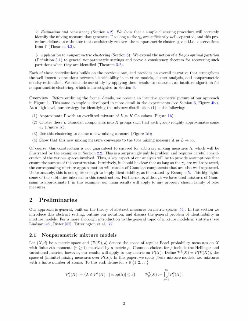
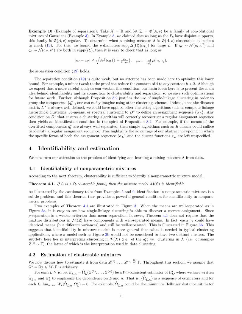
We call the resulting algorithm NPMIX (for N onParametric MIX ture modeling). To illustrate the basicidea, we first implemented four simple one-dimensional models:

(i) GaussGamma (K = 4): A mixture of two Gaussian distributions, one gamma distribution, and aGaussian mixture.

(ii) Gumbel (K = 3): A GMM with three components that has been contaminated with non-Gaussian,Gumbel noise.

(iii) Poly (K = 2): A mixture of two polynomials with non-overlapping supports.

(iv) Sobolev (K = 3): A mixture of three random nonparametric densities, generated from randomexpansions of an orthogonal basis for the Sobolev space H1(R). This is the same example used inFigure 1.

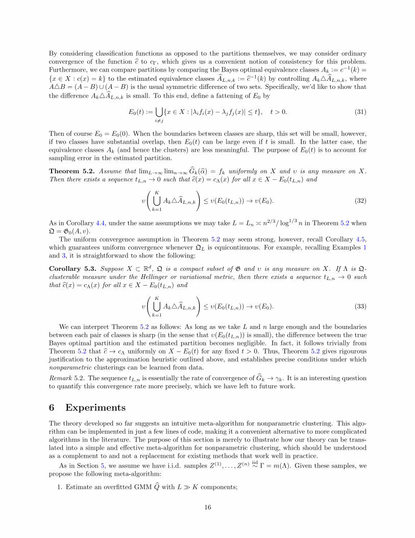
The results are shown in Figure 4. These examples illustrate the basic idea behind the algorithm: Givensamples, overfitted mixture components (depicted by dotted lines in Figure 4) are used to approximate theglobal nonparametric mixture distribution (solid black line). Each of these components is then clustered,with the resulting partition of X = R depicted alongside the true Bayes optimal partition. In each case,cutting the cluster tree to produce K components provides sensible and meaningful approximations to thetrue partitions.

To further validate the proposed algorithm, we implemented the following two-dimensional mixture mod-els and compared the cluster accuracy to existing clustering algorithms on simulated data:

(v) Moons (K = 2): A version of the classical moons dataset in two-dimensions. This model exhibitsa classical failure case of spectral clustering, which is known to have difficulties when clusters areunbalanced (i.e. λ1 6= λ2). For this reason, we ran experiments with both balanced and unbalancedclusters.

(vi) Target (K = 6): A GMM derived from the target dataset (Figure 7). The GMM has 143 compo-nents that are clustered into 6 groups based on the original Target dataset from [73].

Visualizations of the results for our method are shown in Figures 5, 6, and 7. One of the advantages ofour method is the construction of an explicit partition of the entire input space (in this case, X = R2),which is depicted in all three figures. Mixture models are known to occasionally lead to unintuitive clusterassignments in the tails, which we observed with the unbalanced Moons model. This is likely an artifactof the sensitivity of the EM algorithm, and can likely be corrected by using a more robust mixture modelestimator in the first step.

We compared NPMIX against four well-known benchmark algorithms: (i) K-means, (ii) Spectral cluster-ing, (iii) Single-linkage hierarchical clustering, and (iv) A Gaussian mixture model (GMM) with K compo-nents. We only considered methods that classify every sample in a dataset (this precludes, e.g. density-basedclustering). Moreover, of these four algorithms, only K-means and GMM provide a partition of the entireinput space X, which allows for new samples to be classified without re-running the algorithm. All of themethods (including NPMIX) require the specification of the number of clusters K, which was set to the cor-rect number according to the model. In each experiment, we sampled random data from each model and thenused each clustering algorithm to classify each sample. To assess cluster accuracy, we computed the adjusted

17

-10 -5 0 5 10 15 200

0.02

0.04

0.06

0.08

0.1

0.12

0.14

0.16

0.18

0.2

(i) GaussGamma.

-15 -10 -5 0 5 100

0.05

0.1

0.15

0.2

0.25

(ii) Gumbel.

-6 -5 -4 -3 -2 -1 0 1 2 30

0.05

0.1

0.15

0.2

0.25

0.3

0.35

0.4

0.45

(iii) Poly.

-10 -5 0 5 10 15 20 25 300

0.02

0.04

0.06

0.08

0.1

0.12

(iv) Sobolev.

Figure 4: Examples (i)-(iv) of one-dimensional mixture models. The original mixture density is depictedas a solid black line, with the overfitted Gaussian mixture components as dotted lines, coloured accordingto the cluster they are assigned to. The true Bayes optimal partition π and the estimated partition π aredepicted by the horizontal lines at the top, and the raw data are plotted on the x-axis for reference.

RAND index (ARI) for the clustering returned by each method. ARI is a standard permutation-invariantmeasure of cluster accuracy in the literature.

The results are shown in Table 1. On the unbalanced Moons data, NPMIX clearly outperformed each ofthe four existing methods. On balanced data, K-means, spectral clustering, and GMM improved significantly,with spectral clustering performing quite well on average. All four algorithms were still outperformed by

18

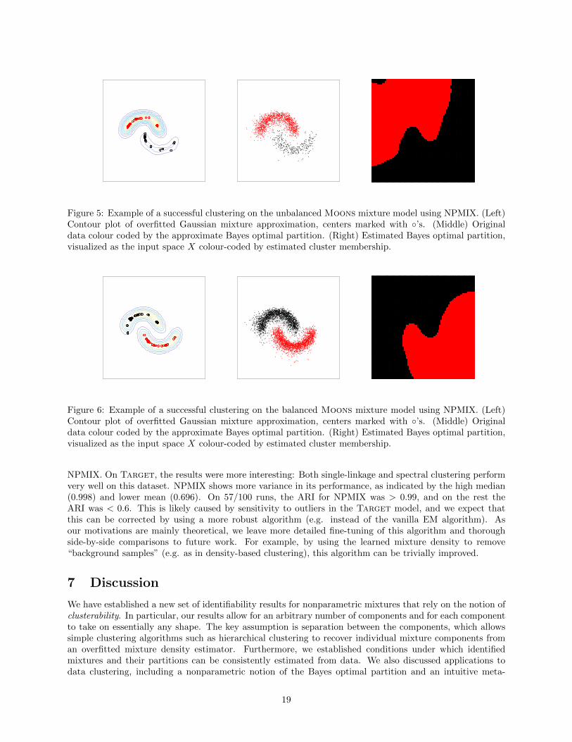
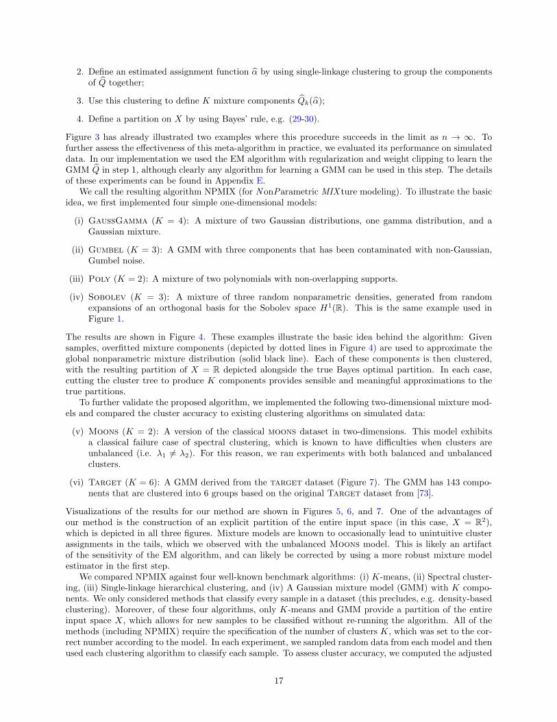
Figure 5: Example of a successful clustering on the unbalanced Moons mixture model using NPMIX. (Left)Contour plot of overfitted Gaussian mixture approximation, centers marked with ’s. (Middle) Originaldata colour coded by the approximate Bayes optimal partition. (Right) Estimated Bayes optimal partition,visualized as the input space X colour-coded by estimated cluster membership.

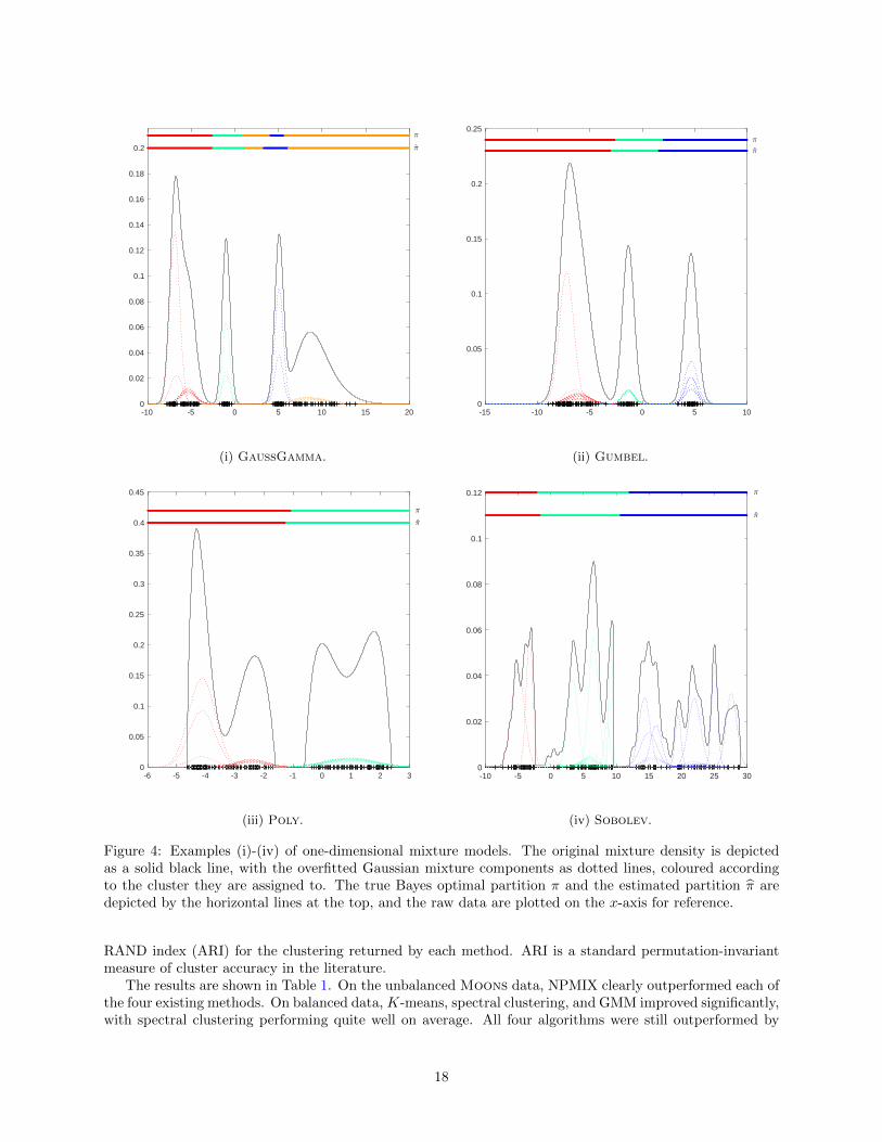
Figure 6: Example of a successful clustering on the balanced Moons mixture model using NPMIX. (Left)Contour plot of overfitted Gaussian mixture approximation, centers marked with ’s. (Middle) Originaldata colour coded by the approximate Bayes optimal partition. (Right) Estimated Bayes optimal partition,visualized as the input space X colour-coded by estimated cluster membership.

NPMIX. On Target, the results were more interesting: Both single-linkage and spectral clustering performvery well on this dataset. NPMIX shows more variance in its performance, as indicated by the high median(0.998) and lower mean (0.696). On 57/100 runs, the ARI for NPMIX was > 0.99, and on the rest theARI was < 0.6. This is likely caused by sensitivity to outliers in the Target model, and we expect thatthis can be corrected by using a more robust algorithm (e.g. instead of the vanilla EM algorithm). Asour motivations are mainly theoretical, we leave more detailed fine-tuning of this algorithm and thoroughside-by-side comparisons to future work. For example, by using the learned mixture density to remove“background samples” (e.g. as in density-based clustering), this algorithm can be trivially improved.

7 Discussion

We have established a new set of identifiability results for nonparametric mixtures that rely on the notion ofclusterability. In particular, our results allow for an arbitrary number of components and for each componentto take on essentially any shape. The key assumption is separation between the components, which allowssimple clustering algorithms such as hierarchical clustering to recover individual mixture components froman overfitted mixture density estimator. Furthermore, we established conditions under which identifiedmixtures and their partitions can be consistently estimated from data. We also discussed applications todata clustering, including a nonparametric notion of the Bayes optimal partition and an intuitive meta-

19

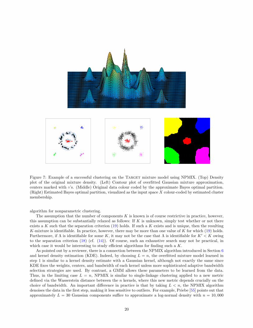
Figure 7: Example of a successful clustering on the Target mixture model using NPMIX. (Top) Densityplot of the original mixture density. (Left) Contour plot of overfitted Gaussian mixture approximation,centers marked with ’s. (Middle) Original data colour coded by the approximate Bayes optimal partition.(Right) Estimated Bayes optimal partition, visualized as the input space X colour-coded by estimated clustermembership.

algorithm for nonparametric clustering.The assumption that the number of components K is known is of course restrictive in practice, however,

this assumption can be substantially relaxed as follows: If K is unknown, simply test whether or not thereexists a K such that the separation criterion (19) holds. If such a K exists and is unique, then the resultingK-mixture is identifiable. In practice, however, there may be more than one value of K for which (19) holds.Furthermore, if Λ is identifiable for some K, it may not be the case that Λ is identifiable for K ′ < K owingto the separation criterion (18) (cf. (14)). Of course, such an exhaustive search may not be practical, inwhich case it would be interesting to study efficient algorithms for finding such a K.

As pointed out by a reviewer, there is a connection between the NPMIX algorithm introduced in Section 6and kernel density estimation (KDE). Indeed, by choosing L = n, the overfitted mixture model learned instep 1 is similar to a kernel density estimate with a Gaussian kernel, although not exactly the same sinceKDE fixes the weights, centers, and bandwidth of each kernel unless more sophisticated adaptive bandwidthselection strategies are used. By contrast, a GMM allows these parameters to be learned from the data.Thus, in the limiting case L = n, NPMIX is similar to single-linkage clustering applied to a new metricdefined via the Wasserstein distance between the n kernels, where this new metric depends crucially on thechoice of bandwidth. An important difference in practice is that by taking L < n, the NPMIX algorithmdenoises the data in the first step, making it less sensitive to outliers. For example, Priebe [55] points out thatapproximately L = 30 Gaussian components suffice to approximate a log-normal density with n = 10, 000

20

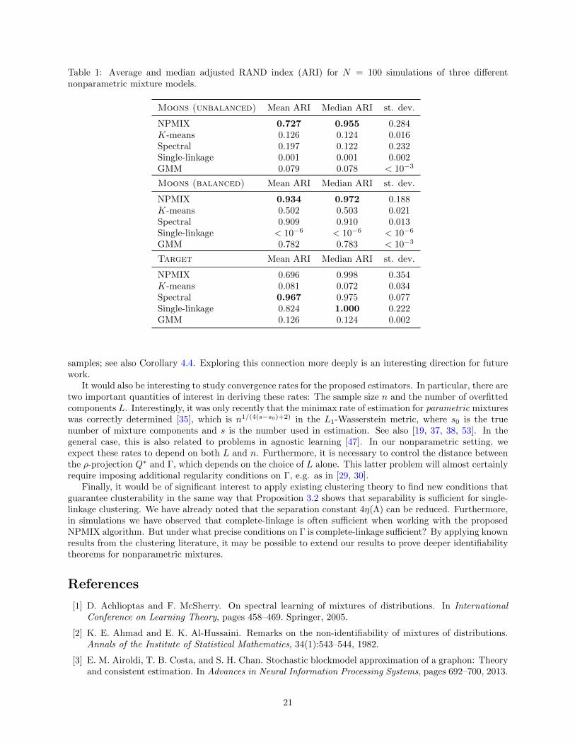
Table 1: Average and median adjusted RAND index (ARI) for N = 100 simulations of three differentnonparametric mixture models.

Moons (unbalanced) Mean ARI Median ARI st. dev.

NPMIX 0.727 0.955 0.284K-means 0.126 0.124 0.016Spectral 0.197 0.122 0.232Single-linkage 0.001 0.001 0.002GMM 0.079 0.078 < 10−3

Moons (balanced) Mean ARI Median ARI st. dev.

NPMIX 0.934 0.972 0.188K-means 0.502 0.503 0.021Spectral 0.909 0.910 0.013Single-linkage < 10−6 < 10−6 < 10−6

GMM 0.782 0.783 < 10−3

Target Mean ARI Median ARI st. dev.

NPMIX 0.696 0.998 0.354K-means 0.081 0.072 0.034Spectral 0.967 0.975 0.077Single-linkage 0.824 1.000 0.222GMM 0.126 0.124 0.002

samples; see also Corollary 4.4. Exploring this connection more deeply is an interesting direction for futurework.

It would also be interesting to study convergence rates for the proposed estimators. In particular, there aretwo important quantities of interest in deriving these rates: The sample size n and the number of overfittedcomponents L. Interestingly, it was only recently that the minimax rate of estimation for parametric mixtureswas correctly determined [35], which is n1/(4(s−s0)+2) in the L1-Wasserstein metric, where s0 is the truenumber of mixture components and s is the number used in estimation. See also [19, 37, 38, 53]. In thegeneral case, this is also related to problems in agnostic learning [47]. In our nonparametric setting, weexpect these rates to depend on both L and n. Furthermore, it is necessary to control the distance betweenthe ρ-projection Q∗ and Γ, which depends on the choice of L alone. This latter problem will almost certainlyrequire imposing additional regularity conditions on Γ, e.g. as in [29, 30].

Finally, it would be of significant interest to apply existing clustering theory to find new conditions thatguarantee clusterability in the same way that Proposition 3.2 shows that separability is sufficient for single-linkage clustering. We have already noted that the separation constant 4η(Λ) can be reduced. Furthermore,in simulations we have observed that complete-linkage is often sufficient when working with the proposedNPMIX algorithm. But under what precise conditions on Γ is complete-linkage sufficient? By applying knownresults from the clustering literature, it may be possible to extend our results to prove deeper identifiabilitytheorems for nonparametric mixtures.

References

[1] D. Achlioptas and F. McSherry. On spectral learning of mixtures of distributions. In InternationalConference on Learning Theory, pages 458–469. Springer, 2005.

[2] K. E. Ahmad and E. K. Al-Hussaini. Remarks on the non-identifiability of mixtures of distributions.Annals of the Institute of Statistical Mathematics, 34(1):543–544, 1982.

[3] E. M. Airoldi, T. B. Costa, and S. H. Chan. Stochastic blockmodel approximation of a graphon: Theoryand consistent estimation. In Advances in Neural Information Processing Systems, pages 692–700, 2013.

21

[4] E. S. Allman, C. Matias, and J. A. Rhodes. Identifiability of parameters in latent structure models withmany observed variables. Annals of Statistics, pages 3099–3132, 2009.

[5] A. Anandkumar, D. Hsu, A. Javanmard, and S. Kakade. Learning linear Bayesian networks with latentvariables. In Proceedings of The 30th International Conference on Machine Learning, pages 249–257,2013.

[6] A. Anandkumar, D. Hsu, M. Janzamin, and S. Kakade. When are overcomplete topic models identifi-able? uniqueness of tensor tucker decompositions with structured sparsity. Journal of Machine LearningResearch, 16:2643–2694, 2015.

[7] S. Arora and R. Kannan. Learning mixtures of separated nonspherical gaussians. Annals of AppliedProbability, pages 69–92, 2005.

[8] O. Barndorff-Nielsen. Identifiability of mixtures of exponential families. Journal of Mathematical Anal-ysis and Applications, 12(1):115–121, 1965.

[9] A. Basu, H. Shioya, and C. Park. Statistical inference: the minimum distance approach. CRC Press,2011.

[10] R. Beran. Minimum hellinger distance estimates for parametric models. Annals of Statistics, pages445–463, 1977.

[11] H. H. Bock. Probabilistic models in cluster analysis. Computational Statistics & Data Analysis, 23(1):5–28, 1996.

[12] S. Bonhomme, K. Jochmans, and J.-M. Robin. Estimating multivariate latent-structure models. Annalsof Statistics, 44(2):540–563, 2016.

[13] S. Bonhomme, K. Jochmans, and J.-M. Robin. Non-parametric estimation of finite mixtures fromrepeated measurements. Journal of the Royal Statistical Society: Series B (Statistical Methodology), 78(1):211–229, 2016.

[14] L. Bordes, S. Mottelet, and P. Vandekerkhove. Semiparametric estimation of a two-component mixturemodel. Annals of Statistics, 34(3):1204–1232, 2006.

[15] L. Bordes, I. Kojadinovic, and P. Vandekerkhove. Semiparametric estimation of a two-componentmixture of linear regressions in which one component is known. Electronic Journal of Statistics, 7:2603–2644, 2013.

[16] C. Bruni, G. Koch, et al. Identifiability of continuous mixtures of unknown gaussian distributions. TheAnnals of Probability, 13(4):1341–1357, 1985.

[17] J. E. Chacon. A population background for nonparametric density-based clustering. Statistical Science,30(4):518–532, 2015.

[18] K. Chaudhuri and S. Dasgupta. Rates of convergence for the cluster tree. In Advances in NeuralInformation Processing Systems, pages 343–351, 2010.

[19] J. Chen. Optimal rate of convergence for finite mixture models. Annals of Statistics, pages 221–233,1995.

[20] Y.-C. Chen, C. R. Genovese, and L. Wasserman. A comprehensive approach to mode clustering. Elec-tronic Journal of Statistics, 10(1):210–241, 2016.

[21] I. Csiszar. Information-type measures of difference of probability distributions and indirect observation.studia scientiarum Mathematicarum Hungarica, 2:229–318, 1967.

[22] A. Cuevas and W. Gonzalez-Manteiga. Data-driven smoothing based on convexity properties. InNonparametric Functional Estimation and Related Topics, pages 225–240. Springer, 1991.

[23] S. Dasgupta. Learning mixtures of gaussians. In Foundations of Computer Science, 1999. 40th AnnualSymposium on, pages 634–644. IEEE, 1999.

[24] L. Devroye, L. Gyorfi, and G. Lugosi. A probabilistic theory of pattern recognition, volume 31. SpringerScience &amp; Business Media, 2013.

22

[25] X. D’Haultfœuille and P. Fevrier. Identification of mixture models using support variations. Journal ofEconometrics, 189(1):70–82, 2015.

[26] J. Eldridge, M. Belkin, and Y. Wang. Graphons, mergeons, and so on! In Advances in Neural Infor-mation Processing Systems, pages 2307–2315, 2016.

[27] C. Fraley and A. E. Raftery. Model-based clustering, discriminant analysis, and density estimation.Journal of the American statistical Association, 97(458):611–631, 2002.

[28] E. Gassiat and J. Rousseau. Non parametric finite translation mixtures with dependent regime. arXivpreprint arXiv:1302.2345, 2013.

[29] C. R. Genovese and L. Wasserman. Rates of convergence for the gaussian mixture sieve. Annals ofStatistics, pages 1105–1127, 2000.

[30] S. Ghosal, A. W. Van Der Vaart, et al. Entropies and rates of convergence for maximum likelihood andbayes estimation for mixtures of normal densities. Annals of Statistics, 29(5):1233–1263, 2001.

[31] P. Hall and X.-H. Zhou. Nonparametric estimation of component distributions in a multivariate mixture.Annals of Statistics, pages 201–224, 2003.

[32] P. Hall, A. Neeman, R. Pakyari, and R. Elmore. Nonparametric inference in multivariate mixtures.Biometrika, 92(3):667–678, 2005.

[33] J. A. Hartigan. Clustering algorithms, volume 209. Wiley New York, 1975.

[34] J. A. Hartigan. Consistency of single linkage for high-density clusters. Journal of the American StatisticalAssociation, 76(374):388–394, 1981.

[35] P. Heinrich and J. Kahn. Strong identifiability and optimal minimax rates for finite mixture estimation.Annals of Statistics, 46(6A):2844–2870, 2018. doi: 10.1214/17-AOS1641. cited By 1.

[36] T. Hettmansperger and H. Thomas. Almost nonparametric inference for repeated measures in mixturemodels. Journal of the Royal Statistical Society: Series B (Statistical Methodology), 62(4):811–825,2000.

[37] N. Ho and X. Nguyen. On strong identifiability and convergence rates of parameter estimation in finitemixtures. Electronic Journal of Statistics, 10(1):271–307, 2016. doi: 10.1214/16-EJS1105. cited By 2.

[38] N. Ho and X. Nguyen. Singularity structures and impacts on parameter estimation in finite mixturesof distributions. arXiv preprint arXiv:1609.02655, 2016.

[39] P. W. Holland, K. B. Laskey, and S. Leinhardt. Stochastic blockmodels: First steps. Social networks,5(2):109–137, 1983.

[40] H. Holzmann, A. Munk, and T. Gneiting. Identifiability of finite mixtures of elliptical distributions.Scandinavian journal of statistics, 33(4):753–763, 2006.

[41] D. R. Hunter and D. S. Young. Semiparametric mixtures of regressions. Journal of NonparametricStatistics, 24(1):19–38, 2012.

[42] D. R. Hunter, S. Wang, and T. P. Hettmansperger. Inference for mixtures of symmetric distributions.Annals of Statistics, pages 224–251, 2007.

[43] R. A. Jacobs, M. I. Jordan, S. J. Nowlan, and G. E. Hinton. Adaptive mixtures of local experts. Neuralcomputation, 3(1):79–87, 1991.

[44] K. Jochmans, M. Henry, and B. Salanie. Inference on two-component mixtures under tail restrictions.Econometric Theory, 33(3):610–635, 2017.

[45] R. Kannan, H. Salmasian, and S. Vempala. The spectral method for general mixture models. SIAMJournal on Computing, 38(3):1141–1156, 2008.

[46] M. Levine, D. R. Hunter, and D. Chauveau. Maximum smoothed likelihood for multivariate mixtures.Biometrika, pages 403–416, 2011.

[47] J. Li and L. Schmidt. A nearly optimal and agnostic algorithm for properly learning a mixture of k

23

gaussians, for any constant k. arXiv preprint arXiv:1506.01367, 2015.

[48] B. G. Lindsay. Mixture models: theory, geometry and applications. In NSF-CBMS regional conferenceseries in probability and statistics, pages i–163. JSTOR, 1995.

[49] S. Lloyd. Least squares quantization in pcm. IEEE transactions on information theory, 28(2):129–137,1982.

[50] J. MacQueen. Some methods for classification and analysis of multivariate observations. In Proceedingsof the fifth Berkeley symposium on mathematical statistics and probability, volume 1, pages 281–297.Oakland, CA, USA, 1967.

[51] D. G. Mixon, S. Villar, and R. Ward. Clustering subgaussian mixtures by semidefinite programming.Information and Inference: A Journal of the IMA, 6(4):389–415, 2017.

[52] A. Y. Ng, M. I. Jordan, and Y. Weiss. On spectral clustering: Analysis and an algorithm. In NIPS,volume 14, pages 849–856, 2001.

[53] X. Nguyen. Convergence of latent mixing measures in finite and infinite mixture models. Annals ofStatistics, 41(1):370–400, 2013.

[54] K. R. Parthasarathy. Probability measures on metric spaces, volume 352. American Mathematical Soc.,1967.

[55] C. E. Priebe. Adaptive mixtures. Journal of the American Statistical Association, 89(427):796–806,1994.

[56] A. Rinaldo and L. Wasserman. Generalized density clustering. Annals of Statistics, pages 2678–2722,2010.

[57] G. Ritter. Robust cluster analysis and variable selection. CRC Press, 2014.

[58] K. Rohe, S. Chatterjee, and B. Yu. Spectral clustering and the high-dimensional stochastic blockmodel.Annals of Statistics, 39(4):1878–1915, 2011.

[59] G. Schiebinger, M. J. Wainwright, and B. Yu. The geometry of kernelized spectral clustering. Annalsof Statistics, 43(2):819–846, 2015.

[60] T. Shi, M. Belkin, and B. Yu. Data spectroscopy: Eigenspaces of convolution operators and clustering.Annals of Statistics, pages 3960–3984, 2009.

[61] B. Sriperumbudur and I. Steinwart. Consistency and rates for clustering with dbscan. In ArtificialIntelligence and Statistics, pages 1090–1098, 2012.

[62] H. Steinhaus. Sur la division des corp materiels en parties. Bull. Acad. Polon. Sci, 1(804):801, 1956.

[63] I. Steinwart. Adaptive density level set clustering. In International Conference on Learning Theory,pages 703–738, 2011.

[64] I. Steinwart. Fully adaptive density-based clustering. Annals of Statistics, 43(5):2132–2167, 2015.

[65] T. Sweeting. On a converse to scheffe’s theorem. Annals of Statistics, 14(3):1252–1256, 1986.

[66] J. Tang, Z. Meng, X. Nguyen, Q. Mei, and M. Zhang. Understanding the limiting factors of topicmodeling via posterior contraction analysis. In International Conference on Machine Learning, pages190–198, 2014.

[67] H. Teicher. On the mixture of distributions. The Annals of Mathematical Statistics, pages 55–73, 1960.

[68] H. Teicher. Identifiability of mixtures. The annals of Mathematical statistics, 32(1):244–248, 1961.

[69] H. Teicher. Identifiability of finite mixtures. The annals of Mathematical statistics, pages 1265–1269,1963.

[70] H. Teicher. Identifiability of mixtures of product measures. The Annals of Mathematical Statistics, 38(4):1300–1302, 1967.

[71] P. Thomann, I. Steinwart, and N. Schmid. Towards an axiomatic approach to hierarchical clustering of

24

measures. Journal of Machine Learning Research, 16:1949–2002, 2015.

[72] D. M. Titterington, A. F. Smith, and U. E. Makov. Statistical analysis of finite mixture distributions.Wiley,, 1985.

[73] A. Ultsch. Clustering with SOM: U*C. In Proc. Workshop on Self-Organizing Maps, Paris, France,pages 75–82, 2005. URL https://www.uni-marburg.de/fb12/arbeitsgruppen/datenbionik/data.

[74] J. H. Wolfe. Pattern clustering by multivariate mixture analysis. Multivariate Behavioral Research, 5(3):329–350, 1970.

[75] S. J. Yakowitz and J. D. Spragins. On the identifiability of finite mixtures. The Annals of MathematicalStatistics, pages 209–214, 1968.

[76] D. Yan, L. Huang, and M. I. Jordan. Fast approximate spectral clustering. In Proceedings of the15th ACM SIGKDD international conference on Knowledge discovery and data mining, pages 907–916.ACM, 2009.

A Proofs

Throughout these appendices, we denote the Hellinger metric on P(X) by ρH and similarly the variational(a.k.a. total variation) distance by ρTV.

A.1 Proof of Lemma 3.1

Fix ε > 0 and let Pk,ε ∈ P20 (Q) be such that ρTV(m(Pk,ε), γk) < ε/K. Define E := ∪Kk=1 supp(Pk,ε) and

let gε,` ∼ N (µε,`,Σε,`) (` = 1, . . . , L) be an enumeration of E. If each gε,` is distinct, then we are done.Suppose to the contrary that gε,` = gε,`′ for some `′ 6= `. Let t > 0 be so small that B(µε,`, t) ∩ E = µε,`for all `. Then we can find δ` 6= δ`′ ∈ B(µε,`, t) such that µε,` + δ` 6= µε,`′ + δ`′ . If there are multiple suchatoms, repeat this process until there are no shared atoms. Let δ = (δ1, . . . , δL) and define Pk,ε,δ to be equalto Pk,ε except that gε,` is replaced with N (µε,` + δ`,Σε,`). Evidently, it is clear from this construction that

ρTV(m(Pk,ε,δ), γk)→ 0 as ε, t→ 0. Defining Pε :=∑Kk=1 λkPε,k,δ, we have Wr(Pε,Λ)→ 0.

It remains to show that Pε is G-regular. It is clear that the ρTV-projection exists and is unique forL ≥ |E| (i.e. since Γ ∈M(GL)), which establishes Definition 3.1(a). To see Definition 3.1(b), one may checkthat the assignment sequence given by αL(`) = k ⇐⇒ gε,` ∈ supp(Pk,ε,δ) works.

A.2 Some metric inequalities

Throughout this section, we assume that L and α are fixed. Thus we will often suppress the dependence onL and α, writing Ω∗k = Ω∗k(α), Q∗k = Q∗k(α), and so on. We will also write q∗` ∈ Q∗k ⇐⇒ α(`) = k ⇐⇒q∗` ∈ supp(Ω∗k).

Next, we introduce some new notation. Define

η(t) := supk

∆(Ω∗k) + t. (34)

and

ε = εL,n := sup`ρ(q`, q

∗` ), δ = δL := sup

kρ(Q∗k, γk). (35)

Recall the following assumptions, which are restated here for reference in the proofs:

(B1) ρ(γi, γj) ≥ 4η(δ) for i 6= j;

(B2) There is an assignment map such that ρ(Q∗k, γk) < δ for each k;

(B3) q` ∈ B(q∗` , ε) for all `.

(B1) is (19), (B2) is Definition 3.1(b), and (B3) is (35).

25

Lemma A.1. Let δ > 0 and ε > 0 be arbitrary. Under (B1)-(B3), the following are true:

(M1) ρ(q∗` , γk) ≤ η(δ) if q∗` ∈ Q∗k;

(M2) ρ(q`, γk) ≤ η(δ + ε) if q∗` ∈ Q∗k;

(M3) ρ(q∗` , γi) ≥ 3η(δ) if q∗` /∈ Q∗i ;

(M4) ρ(q`, γi) ≥ 3η(δ)− ε if q∗` /∈ Q∗i ;

Proof. We prove each claim in order below.

(M1): Using (B2), we have

ρ(γk, q∗` ) ≤ ρ(γk, Q

∗k) + ρ(Q∗k, q

∗` )

≤ δ + ∆(Ω∗k)

≤ η(δ).

(M2): Invoking both (B3) and (M1), we have ρ(q`, γk) ≤ ρ(q`, q∗` ) + ρ(q∗` , γk) ≤ ε+ η(δ) = η(δ + ε).

(M3): Let k be the index such that q∗` ∈ Q∗k. Then, via the reverse triangle inequality,

η(δ)(M1)

≥ ρ(γk, q∗` ) ≥ ρ(γk, γi)− ρ(γi, q

∗` )

(B1)

≥ 4η(δ)− ρ(γi, q∗` ),

and the desired result follows after re-arrangement.

(M4): Same as the proof of (M3), except invoke (M2) in place of (M1).

The previous lemma bounded the distance between q∗` , q` and the true nonparametric measure γk. Thenext lemma leverages the previous one to bound the distances between pairs of overfitted components andtheir estimates.

Lemma A.2. Let δ > 0 and ε > 0 be arbitrary. Under (B1)-(B3), the following are true:

(M5) ρ(q∗` , q∗`′) ≤ η(δ) if q∗` , q

∗`′ ∈ Q∗k;

(M6) ρ(q`, q`′) ≤ η(2ε) if q∗` , q∗`′ ∈ Q∗k;

(M7) If q∗` ∈ Q∗k and q∗`′ ∈ Q∗k′ , k 6= k′, then ρ(q∗` , q∗`′) ≥ 2η(δ).

(M8) If q∗` ∈ Q∗k and q∗`′ ∈ Q∗k′ , k 6= k′, then ρ(q`, q`′) ≥ 2η(δ)− ε.

Proof. We prove each claim in order below.

(M5): Since q∗` , q∗`′ ∈ Q∗k it follows by definition that q∗` , q

∗`′ ∈ supp(Ω∗k). But then ρ(q∗i , q

∗j ) ≤ ∆(Ω∗k) ≤ η(δ).

(M6): As in the proof of (M5), we have ρ(q`, q`′) ≤ ∆(Ω∗k) and hence

ρ(q`, q`′) ≤ ρ(q`, q`) + ρ(q`, q`′) + ρ(q`′ , q`′) ≤ 2ε+ ∆(Ω∗k) ≤ η(2ε).

(M7): We have

ρ(q∗` , q∗`′) ≥ ρ(q∗` , γk′)− ρ(γk′ , q

∗`′)

(M1)

≥ ρ(q∗` , γk′)− η(δ)

and similarly ρ(q∗` , q∗`′) ≥ ρ(q∗`′ , γk)− η(δ). Adding these inequalities,

2ρ(q∗` , q∗`′) ≥ ρ(q∗` , γk′) + ρ(q∗`′ , γk)− 2η(δ)

=⇒ ρ(q∗` , γk′) + ρ(q∗`′ , γk) ≤ 2ρ(q∗` , q∗`′) + 2η(δ).

Invoking (M3) on the left, we have

6η(δ) ≤ ρ(q∗` , γk′) + ρ(q∗`′ , γk) ≤ 2ρ(q∗` , q∗`′) + 2η(δ) ⇐⇒ ρ(q∗` , q

∗`′) ≥ 2η(δ).

(M8): In the proof of (M7), replace (M1) with (M2) and (M3) with (M4).

26

A.3 Proof of Proposition 3.2

By definition, α(i) = α(j) ⇐⇒ q∗i , q∗j ∈ supp(Ω∗k). Note also that η(Ω∗(α)) = η(δ) (cf. (14), (34)) for

δ := supk ρ(Q∗k, γk). Now, if q∗i , q∗j ∈ supp(Ω∗k), then ρ(q∗i , q

∗j ) ≤ η(δ) = η(Ω∗(α)) by (M5) of Lemma A.2.

Conversely, suppose q∗i ∈ supp(Ω∗k) but q∗j ∈ supp(Ω∗k′) with k 6= k′. Then (M7) of Lemma A.2 implies that

ρ(q∗i , q∗j ) ≥ 2η(δ) > η(δ) = η(Ω∗(α)),

which proves (16). The equivalence (17) follows from a similar argument.In particular, (16) and (17) together imply that if α(i) = k = α(j), single-linkage hierarchical clustering

will join components qi and qj before including any component q` such that α(`) 6= k. Thus, cuttingthe resulting dendrogram at any level t ∈ (η(Ω∗(α)), 2η(Ω∗(α))) will produce K clusters corresponding toα−1(1), . . . , α−1(K).

A.4 Proof of Theorem 4.1

We first note the following consequence of regularity (Definition 3.1):

Lemma A.3. If Λ is a regular mixing measure then Wr(Ω∗(αL),Λ)→ 0 as L→∞ for any αL ∈ A∞K (Λ).

Proof. This follows from Definition 3.2 and Lemma C.3.

Proof of Theorem 4.1. Since L is clusterable by assumption, there is a function χL : ML(L)→ AL→K suchthat

limL→∞

ρ(Q∗k(αL), γk) = 0 and limL→∞

|$∗k(αL)− λk| = 0 ∀ k = 1, . . . ,K, (36)

where αL = χL(Ω∗). This defines a function FL :M(L)→ QL→K by

FL(Γ) = Ω∗(αL), where Ω∗ = ML(TL(Γ)) and αL = χL(Ω∗). (37)

The function FL defines a unique, well-defined procedure for associating to a mixture distribution Γ = m(Λ)a mixing measure. Finally, define

h(Γ) := limL→∞

FL(Γ),

where convergence of FL(Γ) is understood to be with respect to the Wasserstein metric Wr. It remains toshow that h(m(Λ)) = Λ for all Λ ∈ L, i.e. Wr(FL(m(Λ)),Λ)→ 0. But this follows from Lemma A.3.

Finally, to show that m is a bijection, we need to show that if m(Λ) = m(Λ′) for some Λ,Λ′ ∈ L, thenΛ = Λ′. We just proved that limL→∞ FL(m(Λ)) = Λ for all Λ ∈ L, and hence

Λ′ = limL→∞

FL(m(Λ′)) = limL→∞

FL(m(Λ)) = Λ.

This proves that m is injective, and surjectivity is obvious since m is onto M(L) by definition. Thus m is abijection as claimed and the proof is complete.

A.5 Proof of Proposition 4.2

Define ∆0 := supk ∆(Ω∗k), so that η(δ) = ∆0 + δ.

Proposition A.4. Suppose that ε > 0 and δ > 0 satisfy

3ε− 2δ < ∆0.

Then under (B1)-(B3) we have ρ(qi, qj) ≤ η(2ε) if and only if ρ(q∗i , q∗j ) ≤ η(δ).

27

Proof. Suppose ρ(q∗i , q∗j ) ≤ η(δ), which implies α(i) = α(j) by Proposition 3.2. Then (M6) of Lemma A.2

implies ρ(qi, qj) ≤ η(2ε). Conversely, suppose ρ(qi, qj) ≤ η(2ε) but ρ(q∗i , q∗j ) > η(δ). By Proposition 3.2, this

means that α(i) 6= α(j), and invoking (M8) of Lemma A.2 we deduce that ρ(qi, qj) ≥ 2η(δ)− ε. Thus, sincealso ρ(qi, qj) ≤ η(2ε), we have

2η(δ)− ε ≤ ρ(qi, qj) ≤ η(2ε)

⇐⇒ 2∆0 + 2δ − ε ≤ ∆0 + 2ε

⇐⇒ ∆0 ≤ 3ε− 2δ,

which contradicts the assumption that ∆0 > 3ε− 2δ.

Proof of Proposition 4.2. Note that η = η(2ε) and η(Ω∗(α)) = η(δ), so that Propositions A.4 and 3.2 togetherimply ρ(qi, qj) ≤ η(2ε) ⇐⇒ α(i) = α(j). In fact, we also have ρ(qi, qj) ≥ 2η(δ) − ε ⇐⇒ α(i) 6= α(j).Thus, as long as 2η(δ)− ε > η(2ε), single-linkage clustering will recover the K components (i.e. by cuttingthe dendrogram at any t ∈ (η(2ε), 2η(δ)− ε)). But 2η(δ)− ε > η(2ε) ⇐⇒ ∆0 > 3ε− 2δ, which is true byassumption.

A.6 Proof of Theorem 4.3

We first need the following lemma:

Lemma A.5. Assume Ωn,Ω ∈ P2L(X). If Wr(Ω

n,Ω)→ 0 then for any α ∈ AL→K ,

Wr(Ωn(α),Ω(α))→ 0, (38)

ρ(Qnk (α), Qk(α))→ 0, (39)

|$nk (α)−$k(α)| → 0. (40)

Furthermore, each sequence (38), (39), and (40) converges at the same rate as Wr(Ωn,Ω).

Proof. By Lemma C.3, we may assume without loss of generality that ρ(qn` , q`) → 0 and |ωn` − ω`| → 0 atthe same rate as Wr(Ω

n,Ω). Then

$nk (α) =

∑`∈α−1(k)

ωn` →∑

`∈α−1(k)

ω` = $k(α)

and furthermore ωn` /$nk (α) → ω`/$k(α) for each ` at the same rate as Wr(Ω

n,Ω). This proves (40), and(39) follows similarly. In particular, each of the atoms and weights in Ωn(α) converges to an atom and weightin Ω(α). Invoking Lemma C.3 once again, we deduce (38). The proof is complete.

Proof of Theorem 4.3. We first prove Wr(Ω(αL,n),Ω∗(αL)) → 0. By assumption, Ω is a Wr-consistent

estimate of Ω∗, i.e. Wr(Ω,Ω∗)→ 0 as n→∞. Proposition 4.2 implies αL,n = αL, and hence

Wr(Ω(αL,n),Ω∗(αL)) = Wr(Ω(αL),Ω∗(αL))→ 0 (41)

by Lemma A.5. Thus,

Wr(Ω(αL,n),Λ) ≤Wr(Ω(αL,n),Ω∗(αL)) +Wr(Ω∗(αL),Λ)→ 0

by (41) and Lemma A.3. This proves (22), as desired.

Remark A.1. It is interesting to study how L must grow as a function of n in order to achieve consistencyin Theorem 4.3. In fact, since

Wr(Ω(αL,n),Λ) ≤Wr(Ω(αL,n),Ω∗(αL)) +Wr(Ω∗(αL),Λ)

:= ψL,n + ΨL

it is clear that L = Ln is governed by the rate of convergence ψL,n of Wr(Ω(αL,n),Ω∗(αL)). Assuming

αL,n = αL (this follows, e.g. from Proposition 4.2) the convergence rate of Wr(Ω(αL,n),Ω∗(αL)) is the

same as Wr(Ω,Ω∗) by Lemma A.5. Thus, this problem reduces to studying the rate of convergence of the

estimator Ω. Conveniently, by Theorem 2 in Nguyen [53], this can be bounded above as L → ∞ by the

variational distance ρTV(m(Ω(αL,n)),m(Ω∗(αL))).

28

A.7 Proof of Theorem 5.2

Write g∗` for the density of q∗` and G∗ for the density of Q∗, and similarly g` and G for the densities of q`and Q, respectively. To reduce notational overload in the proof, we will suppress the dependence on α (cf.(29)) below. To this end, define

Gk(x) :=1

$k(αL,n)

∑`∈α−1

L,n(k)

ω`g`(x), $k(αL,n) :=∑

`∈α−1L,n(k)

ω`,

G∗k(x) :=1

$∗k(αL)

∑`∈α−1

L (k)

ω∗` g∗` (x), $∗k(αL) :=

∑`∈α−1

L (k)

ω∗` .

Then Gk(x) and G∗k(x) are the densities of Qk(αL,n) and Q∗, respectively.

Lemma A.6. If Gk → fk uniformly on X for each k = 1, . . . ,K, then there exists a sequence tL,n → 0 suchthat cL,n(x) = c(x) for all x ∈ X − E0(tL,n).

Proof. Define

tL,n := 2 supk

supx∈X|Gk(x)− fk(x)| ≥ 0 (42)

and note that tL,n → 0 since Gk → fk uniformly for each k. Then for any x /∈ E0(tL,n) and i 6= j,|fi(x) − fj(x)| > tL,n, which means either fi(x) > fj(x) + tL,n or fj(x) > fi(x) + tL,n. Taking i = c(x), itfollows that

fc(x)(x) > supj 6=c(x)

fj(x) + tL,n ∀x /∈ E0(tL,n). (43)

Thus for any j 6= c(x),

Gc(x)(x)(a)> fc(x)(x)− tL,n

2

(b)> fj(x) +

tL,n2

(c)> Gj(x)

(a) follows from (43); (b) follows from (42), and (c) follows again from (43). It follows that cL,n(x) = c(x)for all x /∈ E0(tL,n), as desired.

Lemma A.7. Under the assumptions of Lemma A.6, it follows that AL,n,k4Ak ⊂ E0(tL,n) for all k =1, . . . ,K. In particular,

K⋃k=1

AL,n,k4Ak ⊂ E0(tL,n).

Proof. Lemma A.6 implies that cL,n(x) = c(x) := k for all x /∈ E0(tL,n). In particular, AL,n,k ∩E0(tL,n)c =

Ak ∩ E0(tL,n)c. Lemma C.1 thus implies that AL,n,k4Ak ⊂ E0(tL,n), as desired.

Proof of Theorem 5.2. This is an immediate consequence of Lemmas A.6 and A.7.

B Examples

In this Appendix, we prove the claims made in Examples 6, 7 and 8 from Section 3.3. Define the followingfamilies of mixing measures:

F1(ζ,K) :=

K∑k=1

λkδγk : γk ζ, λk ≥ 0,

K∑k=1

λk = 1

, (44)

F2(Q,K) :=

K∑k=1

λkδm(Pk) : Pk ∈ Q, λk ≥ 0,

K∑k=1

λk = 1

. (45)

Here, ζ ∈ P(X) is a fixed dominating measure and Q ⊂ P2(X) is a Borel set.

29

B.1 Disjoint mixtures

The family F1(ζ,K) defined in (44) corresponds to Example 6. For any Λ ∈ F1(ζ,K), let F =∑Kk=1 λkfk

denote the density of Γ = m(Λ). Let G′ ⊂ G be a compact set of Gaussian mixtures and G∗L =∑L`=1 ω

∗` g∗`

be a corresponding ρTV-projection onto M(G′L), with g∗` ∼ N (a∗` , v∗` ).

The following lemma implies G′-regularity of Λ as long as the fk have disjoint supports:

Lemma B.1. Suppose Λ ∈ F1(ζ,K) and G′ ⊂ G is a compact set such thatM(G′) is dense inM(F1(ζ,K)).Define E := ∪Kk=1Ek and an assignment sequence αL by

αL(`) =

k, a∗` ∈ Ek,1, a∗` ∈ Ec.

If the Ek are disjoint, then $∗k(αL)→ λk and∥∥G∗k(αL)− fk

∥∥1→ 0 for each k.

Remark B.1. As the proof indicates, the conclusion of Lemma B.1 remains true if G′ is not compact (e.g.if G′ = G), however, in this case the ρTV-projection may not be well-defined. In this case, the conclusionholds for any G∗L ∈ M(GL) such that ρTV(G∗L, F ) → 0 as L → ∞. Furthermore, the assumption that

M(G′) =M(F1(ζ,K)) can be trivially relaxed to the requirement that F ∈M(G′) ∩M(F1(ζ,K)).

Proof of Lemma B.1. To reduce notational clutter, we omit the index L and write αK = α and G∗L = G∗.We have

‖G∗ − F‖1 =

K∑k=1

ż

Ek

|G∗ − F | dζ +

ż

Ec

G∗ dζ

=

K∑k=1

ż

Ek

|∑j 6=k

$∗j (α)G∗j (α)︸ ︷︷ ︸:=hk,L

+$∗k(α)G∗k(α)− λkfk︸ ︷︷ ︸:=−gk,L

| dζ +

ż

Ec

G∗L dζ

=

K∑k=1

ż

Ek

|hk,L − gk,L| dζ +

ż

Ec

G∗L dζ.

Since ‖G∗ − F‖1 → 0, it follows thatş

Ec G∗ dζ → 0 and hence

ş

Ek$∗j (α)G∗j (α) dζ → 0 for all j 6= k. This is

because off of Ej , $∗j (α)G∗j (α) is monotonic (i.e. decreasing to the right and increasing from the left), which

implies (assuming without loss of generality that cj < bk— i.e. Ej lies to the left of Ek on the real line),

ż ck

bk

$∗j (α)G∗j (α) <

ż bk

cj

$∗j (α)G∗j (α) ≤ż

Ec

G∗ → 0.

Furthermore, it follows thatş

Ek|hk,L − gk,L| dζ → 0 for each k, which implies

ş

Ek|gk,L| dζ → 0 since

ż

Ek

|gk,L| dζ −ż

Ek

|hk,L| dζ ≤ż

Ek

|hk,L − gk,L| dζ → 0.

Thusż

Ek

|$∗k(α)G∗k(α)− λkfk| dζ → 0 ∀k,

i.e. $∗k(α)G∗k(α)→ λkfk in L1 (on Ek), which implies∣∣∣ żEk

$∗k(α)G∗k(α)− λkfk

dζ∣∣∣ =

∣∣∣$∗k(α)

ż

Ek

G∗k(α) dζ − λk∣∣∣→ 0.

However, sinceş

Ec Q∗L dζ → 0, we have

ş

EckG∗k(α) dζ → 0 and hence also

ş

EkG∗k(α) dζ → 1. It follows that

$∗k(α)→ λk and similarly∥∥G∗k(α)− fk

∥∥1→ 0, as desired.

30

B.2 Mixtures of finite mixtures

By restricting to finite mixtures Q0, the family F2(Q0,K) defined in (45) corresponds to Example 7. Thefollowing lemma establishes Q-regularity of this family.

Lemma B.2. Suppose Q ⊂ P2(X) satisfies Condition (A) and Λ ∈ F2(Q0,K). If the Pk have disjointsupports, then Λ is Q-regular under any metric ρ.

Proof. Let Λ ∈ F2(Q0; K) and define L0 :=∑Kk=1 | supp(Pk)|. For any L ≥ L0, the ρ-projection of Γ onto

M(QL) is Q∗ = Γ since Γ ∈ M(QL) and ρ is a metric (i.e. ρ(Q∗,Γ) = 0 ⇐⇒ Q∗ = Γ). This verifies part(a) of Definition 3.1. To verify part (b), first write

Γ = Q∗ =

L0∑`=1

ω∗` q∗` , γk =

∑`∈Bk

ω∗` q∗` .

The set Bk ⊂ [L0] indexes all of the components of Γ that contribute to γk, i.e. Bk = ` ∈ [L0] : q∗` ∈supp(Λk). Now define

α(`) = k ⇐⇒ ` ∈ Bk.

Then clearly Q∗k(α) = γk and $∗k(α) = λk, which establishes (b).

B.3 Infinite mixtures

Suppose Q ⊂ P2(X) is compact and identifiable; i.e. restricted to Q, the canonical map m : Q → P(X) isinjective. Then the family F2(Q,K) defined in (45) corresponds to Example 8. As the following examplesillustrate, this family encompasses a wide range of nonparametric mixtures:

• Parametric mixture components with unbounded support. The family F2(Q0,K) is obviously a specialcase of this family, including mixtures whose components are finite Gaussian mixtures and exponentialfamily mixtures.

• Infinite Gaussian mixtures. Although arbitrary mixtures of Gaussians need not be identifiable [67],convolutional mixtures [53, 67] and mixtures of Gaussians with fixed means are identifiable. Moregenerally, we may allow both the means and variances to vary under certain conditions, see Bruniet al. [16]. If the γk come from any of these general families of Gaussian mixtures, then the resultingnonparametric mixture model is a special case of F2(Q,K).

A mixing measure Λ ∈ F2(Q,K) is of the form∑Kk=1 λkδγk , with γk = m(Pk). Thus Λ uniquely defines a

Q-mixture by P :=∑k λkPk.

Through this subsection we assume that ρ is a ϕ-divergence [21, 53], which we recall means that

ρ(µ, ν) =

ż

X

ϕ( dµ

dν

)dν (46)

for some convex function ϕ. If µ is not absolutely continuous with respect to ν, we adopt the usual conventionthat ρ(µ, ν) = +∞. Examples of ϕ-divergences include the Hellinger and variational metrics.

Recall that m is a map between the metric spaces (P2(X),Wr) and (P(X), ρ). We first record animportant fact regarding the continuity of this map:

Lemma B.3. Suppose Q ⊂ P2(X) is compact and identifiable and ρ is a ϕ-divergence. Then m : Q→ P(X)is 1-Lipschitz continuous, and its inverse is continuous.

Proof. This follows from Lemma 1 in Nguyen [53], noting that the argument applies just as well to arbitrarymeasures µ, ν ∈ P(X). Continuity of the inverse follows from the compactness of Q.

The following lemma establishes Q-regularity of F2(Q,K). Its proof uses the well-known fact that theWasserstein metric metrizes the topology of weak convergence, which we denote by ⇒.

31

Lemma B.4. Suppose Λ ∈ F2(Q,K) and define Bk := supp(Pk). Assume that (a) B1, . . . , BK are disjoint,compact sets and (b) Each Bk is a P -continuity set. Then Λ is Q-regular under any ϕ-divergence.

Proof. Let Q∗L ∈ M(QL) be any ρ-projection of Γ and Ω∗L its corresponding mixing measure. We wish toshow that there exists an assignment sequence αL such that ρ(Q∗k(αL), γk) → 0 and |$∗k(αL) − λk| → 0.By Lemma B.3, it suffices to show that Ω∗L,k(αL) ⇒ Pk and $∗L,k(αL) → λk. Consider the assignmentsequence defined by αL(g) = k if and only if g ∈ Bk. Note that αL does not depend on Ω∗L.

We first note that Ω∗L ⇒ P : This follows again from Lemma B.3 since ρ(m(Ω∗L),m(P )) → 0. Thus,in particular, since Bk is a P -continuity set we have both Ω∗L(· |Bk) ⇒ P (· |Bk) and Ω∗L(Bk) → P (Bk).But Ω∗L,k(αL) = Ω∗L(· |Bk) and by Lemma C.2, we have Pk = P (· |Bk). It follows that Ω∗L,k(αL) ⇒ Pk.Similarly, by Lemma C.2, we have $∗L,k(αL) = Ω∗L(Bk)→ P (Bk) = λk. The proof is complete.

C Technical lemmas

Lemma C.1. A ∩ Zc = B ∩ Zc =⇒ A4B ⊂ Z.

Proof. Suppose x ∈ A4B. There are two cases: (i) x ∈ A − B, (ii) x ∈ B − A. We prove (i); the prooffor (ii) is similar. Suppose x ∈ A − B but also x ∈ Zc. Then x ∈ A ∩ Zc = B ∩ Zc, whence x ∈ B, whichcontradicts (i).

Lemma C.2. Suppose P :=∑k λkPk ∈ P2(X), Bk := supp(Pk), and assume that B1, . . . , BK partition

B := supp(P ). Then Pk = P ( · |Bk) and λk = P (Bk).

Proof. For any Borel set A we have

K∑k=1

P (A ∩Bk) = P (A) =

K∑k=1

λkPk(A).

Choosing A = Bj , we deduce that λj = P (Bj). Then for any A ⊂ Bj , P (A) = λjPj(A) since the Bk form apartition. Using λj = P (Bj) and A ⊂ Bj , this implies that

Pj(A) =P (A)

P (Bj)=P (A ∩Bj)P (Bj)

= P (A |Bj).

Finally, for arbitrary Borel A, we have

Pj(A) = Pj(A ∩Bj) + Pj(A ∩Bcj )︸ ︷︷ ︸=0

(i)= Pj(A ∩Bj)

(ii)= P (A |Bj)

since (i) supp(Pj) = Bj and (ii) A ∩Bj ⊂ Bj .

What follows are standard results on the Wasserstein metric. For completeness, we provide completeproofs here. Let (Θ, d) be a metric space and G =

∑mi=1 piδθi , G

′ =∑mj=1 pjδθ′j be two discrete probability

measures on Θ with m atoms each. Then the definition of the Lr-Wasserstein distance (2) is equivalent tothe following:

Wr(G,G′) = inf

[∑i,j

σijdr(θi, θ

′j)]1/r

: 0 ≤ σij ≤ 1,

∑i,j

σij = 1,∑i

σij = p′j ,∑j

σij = pi

.

In the sequel, we write Gn =∑mi=1 pn,iδθn,i

for a sequence of discrete distributions with exactly m atomseach.

32

Remark C.1. Lemma C.3 below encodes a crucial property of Wr that is needed in the proofs. Thus, in con-trast to ρ which can be any metric on P(X), our results are particular to the Wasserstein distance. Notwith-standing, it is likely that our results can be extended to any metric on P2(X) that satisfies Lemma C.3.

Lemma C.3. Wr(Gn, G)→ 0 if and only if there are permutations τn : [m]→ [m] such that

(a) d(θn,τn(i), θi)→ 0 for each i.

(b) |pn,τn(i) − pi| → 0 for each i.

Proof. The =⇒ direction is Lemma C.4 below. The ⇐= direction follows from Lemma C.5 by noting thatGn and G are invariant to permutations of the index i.

Lemma C.4. If Wr(Gn, G)→ 0 then there are permutations τn : [m]→ [m] such that

(a) d(θn,τn(i), θi)→ 0 for each i.

(b) |pn,τn(i) − pi| → 0 for each i.

Proof. We use the fact that Wasserstein convergence implies weak convergence, which is in turn equivalentto convergence of open sets, i.e. Gn(U)→ G(U) for all open sets U . Choose R > 0 so small that B(θi, R) ∩B(θj , R) = ∅ for all i 6= j, whence G(B(θi, r)) = pi for all 0 < r < R. By weak convergence, we thus havefor each i and any 0 < r < R

Gn(B(θi, r))→ G(B(θi, r)) = pi.

Thus, for sufficiently large n, Gn assigns positive probability to the ball B(θi, r), which means that for eachi there is some j ∈ [k] such that θn,i ∈ B(θj , r). Setting τn(j) = i and taking r → 0 completes the proof.

Lemma C.5. If limn→∞ θn,i = θi and limn→∞ pn,i = pi for each i then Wr(Gn, G)→ 0.

Proof. We use the fact that Wr(Gn, G) → 0 is equivalent to weak convergence plus convergence of the

first r moments. For weak convergence, recall thatş

f dGn =∑ki=1 pn,if(θn,i) and hence for any bounded

continuous f ,

ż

f dGn =

m∑i=1

pn,if(θn,i) −→m∑i=1

pif(θi) =

ż

f dG.

Thus Gn converges weakly to G. Furthermore, for any r ≥ 1,

ż

d(x, x0)r dGn(x) =

m∑i=1

pn,id(θn,i, x0)r −→m∑i=1

pid(θi, x0)r =

ż

d(x, x0)r dG(x).

Thus the first r moments of Gn converge to those of G. It follows that Wr(Gn, G)→ 0.

D Wasserstein consistency of the MHDE

Assume L is fixed; any dependence on L will be suppressed here. Let qφ : φ ∈ Φ be a parametric familyof densities such that Φ is compact, and define

Θ =

θ = (p1, . . . , pL, φ1, . . . , φL) ∈ [0, 1]L × ΦL :

L∑`=1

p` = 1

.

For any θ ∈ Θ, let Qθ denote the mixture distribution defined by θ, and Q the family of mixing measuresinduced by Θ.

Suppose that Q∗ = Qθ∗ =∑L`=1 ω

∗` q∗` is the Hellinger projection of m(Λ) ontoM(Q) and Ω∗ = M(Q∗) ∈

Q, i.e.

ρ(Q∗,m(Λ)) < ρ(Qθ,m(Λ)) ∀ θ 6= θ∗.

33

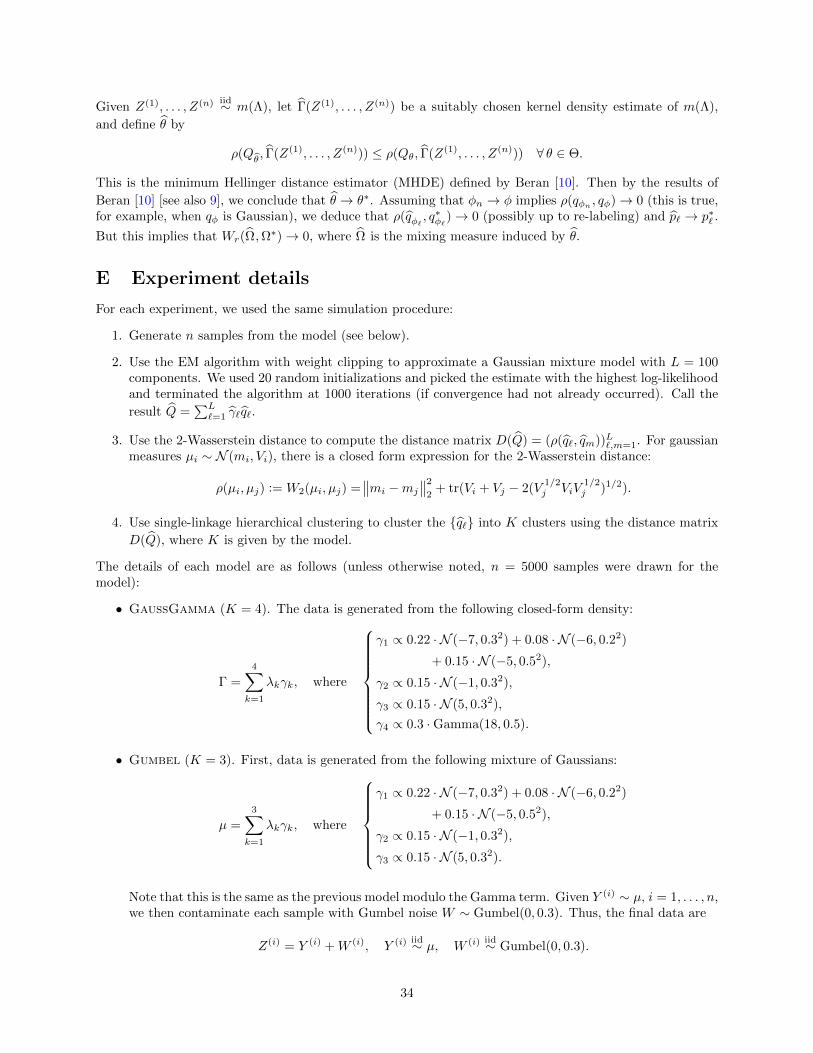
Given Z(1), . . . , Z(n) iid∼ m(Λ), let Γ(Z(1), . . . , Z(n)) be a suitably chosen kernel density estimate of m(Λ),

and define θ by

ρ(Qθ, Γ(Z(1), . . . , Z(n))) ≤ ρ(Qθ, Γ(Z(1), . . . , Z(n))) ∀ θ ∈ Θ.

This is the minimum Hellinger distance estimator (MHDE) defined by Beran [10]. Then by the results of

Beran [10] [see also 9], we conclude that θ → θ∗. Assuming that φn → φ implies ρ(qφn, qφ)→ 0 (this is true,

for example, when qφ is Gaussian), we deduce that ρ(qφ`, q∗φ`

)→ 0 (possibly up to re-labeling) and p` → p∗` .

But this implies that Wr(Ω,Ω∗)→ 0, where Ω is the mixing measure induced by θ.

E Experiment details

For each experiment, we used the same simulation procedure:

1. Generate n samples from the model (see below).

2. Use the EM algorithm with weight clipping to approximate a Gaussian mixture model with L = 100components. We used 20 random initializations and picked the estimate with the highest log-likelihoodand terminated the algorithm at 1000 iterations (if convergence had not already occurred). Call the

result Q =∑L`=1 γ`q`.

3. Use the 2-Wasserstein distance to compute the distance matrix D(Q) = (ρ(q`, qm))L`,m=1. For gaussianmeasures µi ∼ N (mi, Vi), there is a closed form expression for the 2-Wasserstein distance:

ρ(µi, µj) := W2(µi, µj) =∥∥mi −mj

∥∥2

2+ tr(Vi + Vj − 2(V

1/2j ViV

1/2j )1/2).

4. Use single-linkage hierarchical clustering to cluster the q` into K clusters using the distance matrix

D(Q), where K is given by the model.

The details of each model are as follows (unless otherwise noted, n = 5000 samples were drawn for themodel):

• GaussGamma (K = 4). The data is generated from the following closed-form density:

Γ =

4∑k=1

λkγk, where

γ1 ∝ 0.22 · N (−7, 0.32) + 0.08 · N (−6, 0.22)

+ 0.15 · N (−5, 0.52),

γ2 ∝ 0.15 · N (−1, 0.32),

γ3 ∝ 0.15 · N (5, 0.32),

γ4 ∝ 0.3 ·Gamma(18, 0.5).

• Gumbel (K = 3). First, data is generated from the following mixture of Gaussians:

µ =

3∑k=1

λkγk, where

γ1 ∝ 0.22 · N (−7, 0.32) + 0.08 · N (−6, 0.22)

+ 0.15 · N (−5, 0.52),

γ2 ∝ 0.15 · N (−1, 0.32),

γ3 ∝ 0.15 · N (5, 0.32).

Note that this is the same as the previous model modulo the Gamma term. Given Y (i) ∼ µ, i = 1, . . . , n,we then contaminate each sample with Gumbel noise W ∼ Gumbel(0, 0.3). Thus, the final data are

Z(i) = Y (i) +W (i), Y (i) iid∼ µ, W (i) iid∼ Gumbel(0, 0.3).

34

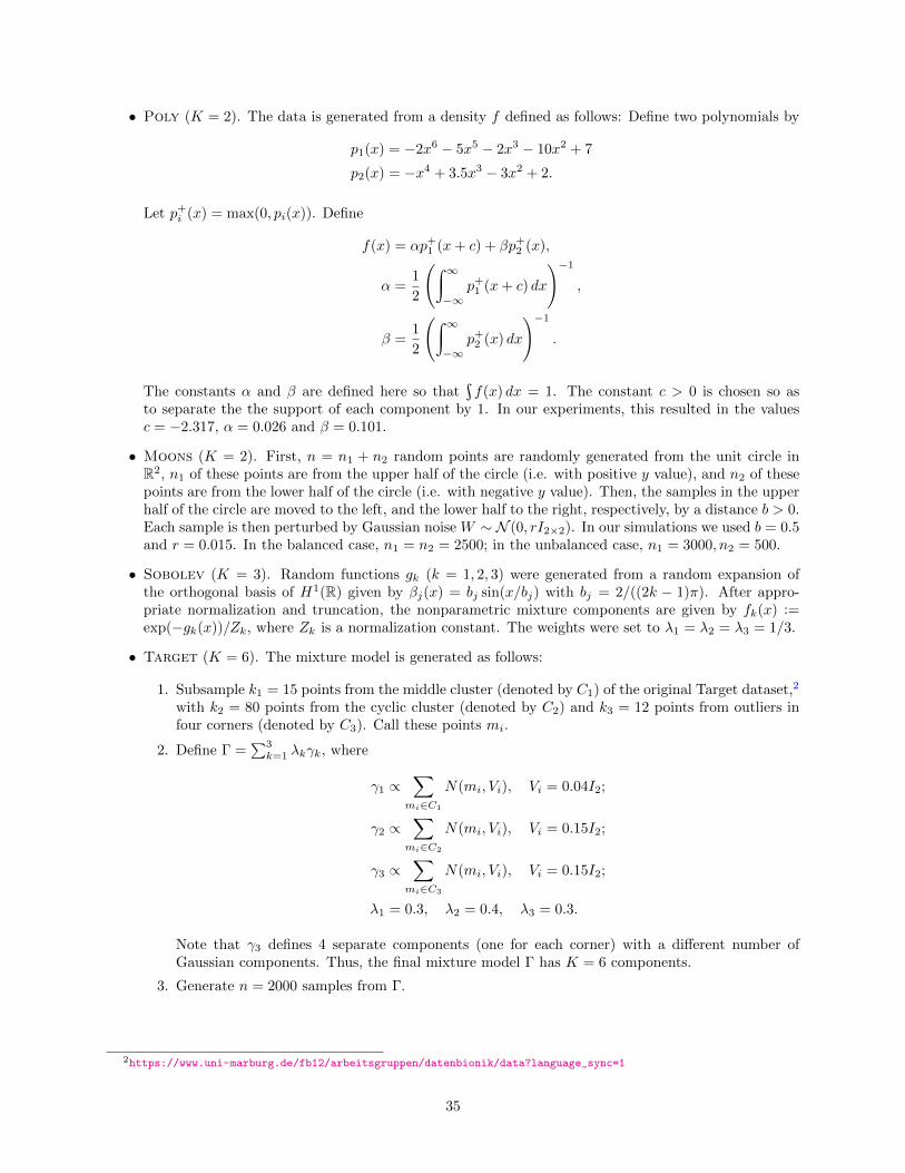
• Poly (K = 2). The data is generated from a density f defined as follows: Define two polynomials by

p1(x) = −2x6 − 5x5 − 2x3 − 10x2 + 7

p2(x) = −x4 + 3.5x3 − 3x2 + 2.

Let p+i (x) = max(0, pi(x)). Define

f(x) = αp+1 (x+ c) + βp+

2 (x),

α =1

2

(ż ∞

−∞p+

1 (x+ c) dx

)−1

,

β =1

2

(ż ∞

−∞p+

2 (x) dx

)−1

.

The constants α and β are defined here so thatş

f(x) dx = 1. The constant c > 0 is chosen so asto separate the the support of each component by 1. In our experiments, this resulted in the valuesc = −2.317, α = 0.026 and β = 0.101.

• Moons (K = 2). First, n = n1 + n2 random points are randomly generated from the unit circle inR2, n1 of these points are from the upper half of the circle (i.e. with positive y value), and n2 of thesepoints are from the lower half of the circle (i.e. with negative y value). Then, the samples in the upperhalf of the circle are moved to the left, and the lower half to the right, respectively, by a distance b > 0.Each sample is then perturbed by Gaussian noise W ∼ N (0, rI2×2). In our simulations we used b = 0.5and r = 0.015. In the balanced case, n1 = n2 = 2500; in the unbalanced case, n1 = 3000, n2 = 500.

• Sobolev (K = 3). Random functions gk (k = 1, 2, 3) were generated from a random expansion ofthe orthogonal basis of H1(R) given by βj(x) = bj sin(x/bj) with bj = 2/((2k − 1)π). After appro-priate normalization and truncation, the nonparametric mixture components are given by fk(x) :=exp(−gk(x))/Zk, where Zk is a normalization constant. The weights were set to λ1 = λ2 = λ3 = 1/3.

• Target (K = 6). The mixture model is generated as follows:

1. Subsample k1 = 15 points from the middle cluster (denoted by C1) of the original Target dataset,2

with k2 = 80 points from the cyclic cluster (denoted by C2) and k3 = 12 points from outliers infour corners (denoted by C3). Call these points mi.

2. Define Γ =∑3k=1 λkγk, where

γ1 ∝∑

mi∈C1

N(mi, Vi), Vi = 0.04I2;

γ2 ∝∑

mi∈C2

N(mi, Vi), Vi = 0.15I2;

γ3 ∝∑

mi∈C3

N(mi, Vi), Vi = 0.15I2;

λ1 = 0.3, λ2 = 0.4, λ3 = 0.3.

Note that γ3 defines 4 separate components (one for each corner) with a different number ofGaussian components. Thus, the final mixture model Γ has K = 6 components.

3. Generate n = 2000 samples from Γ.

2https://www.uni-marburg.de/fb12/arbeitsgruppen/datenbionik/data?language_sync=1

35