BSL PRO Lesson H32 (PDF) - Biopac

Updated 7.20.12

BSL PRO Lesson H32: Heart Rate Variability Analysis

This PRO Lesson describes basic and advanced heart rate variability measurements and details hardware and software setup of the BSL PRO software to record ECG. All data collection and analysis is done via the BIOPAC MP36/MP35/MP30/MP45 data acquisition unit and the Biopac Student Lab PRO software.

Objective

This PRO Lesson will explain statistical measures, geometric measures, and spectral analysis in heart rate variability studies.

Statistical Measures:

NN50 count, PNN50, RMSDD, SDANN, SDSD

Geometric Measures:

HRV triangular index, TINN

Spectral Analysis: 5-min total power (ms), HF (ms2), LF (ms2), HLF morm (n.u.), LF norm (n.u.), LF.HF ratio, VLF (ms2)

Definitions

5-min total power (ms)

Variance of NN intervals over the temporal segment (5 minutes).

HF (ms2) Power in high frequency range (0.15-0.4 Hz)

HF norm (n.u)

HF/(Total Power - VLF) x 100

HRV triangular index

Integral of the density distribution divided by the maximum of the density distribution.

www.biopac.com Page 1 of 16

BSL PRO Lesson H32 BIOPAC Systems, Inc.

LF norm (n.u.)

LF/(Total Power - VLF) X 100

LF/HF ratio LF(ms)/HF(ms)

NN Normal to normal R-R: value of R-R intervals for normal beat. Obtained in real time or post-processing using the Rate function.

NN50 count Number of pairs of adjacent NN intervals differing by more than 50 ms.

pNN50 NN50 count divided by the total number of all NN intervals.

RMSSD Square root of the mean squared differences of successive NN intervals.

SDANN Standard deviation of the average NN interval calculated over short periods: usually 5 minutes. (This lesson is written for 1 minute intervals)

SDSD Standard deviation of differences between adjacent NN.

TINN Baseline width of the distribution measured as a base of a triangle, approximating the NN interval distribution HRV.

For a comprehensive overview, see Guidelines: Heart Rate Variability, European Heart Journal (1996) 17, 354-381.

Equipment

BIOPAC electrode lead set (SS2L) BIOPAC Disposable Electrodes (EL503)—three per subject Electrode gel and abrasive pad (BIOPAC GEL1 and ELPAD) Computer running Windows 7/Vista/XP or Mac OS X Biopac Student Lab PRO software BIOPAC Data Acquisition Unit (MP36/MP35/MP30/MP45)

Setup

Hardware

1. Make sure that the MP unit is off. 2. Turn on the computer. 3. Plug the Electrode Lead (SS2L) into CH 2 on the front of the MP unit.

Software

1. Launch the BSL PRO software. 2. Open the Heart Rate Variability template file by choosing File menu > Open > choose Files of type:

Graph Template (*GTL) > File Name: H32 Heart Rate Variability.gtl.

OR: In BSL 3.7.7 and higher: Launch the Startup Wizard, choose Record a lesson > BSL PRO tab > H32 Heart Rate Variability.gtl.

Calibration

No calibration required.


http://www.escardio.org/guidelines-surveys/esc-guidelines/Scientific_Statements/Documents/guidelines-Heart-Rate-Variability-FT-1996.pdf

http://www.biopac.com/Curriculum/gtl/h32.gtl


Subject

NOTE: A Lead II configuration with electrodes placed directly on the torso will reduce artifact.

1. Remove all substantial metal jewelry from the Subject and make sure that the Subject is not touching any metal (metal pipes, chairs etc.).

2. For best results, lightly abrade the skin with abrasive pads, and put a spot of gel on the electrode contact area.

3. Place three electrodes on the Subject as the table indicates.

Electrode Position Lead Color

Right arm Centered on the anterior wrist (same side as the palm of the hand), about 0.5-1.0” down from the palm

White

Right leg Medial, just above the ankle, flat on skin (not over bone) Black

Left leg Medial, just above the ankle, flat on skin (not over bone) Red

1. Attach the electrode leads by color as shown in the table.

The pinch connectors work like small clothes pins; however, they will attach to the electrode only on one side. You may have to rotate the pin to make sure the metal on the inside of the clip is connected, touching and clamped onto the electrode at the base of the nipple.

Clip connector cables to Subject's clothing, or place so that there is no strain on the electrode clips or the cable wires at any point in the setup.

5. Turn on the MP unit (assuming the AC100A power adapter has already been connected). 6. Wait 5 minutes after the electrodes have been attached to the skin to begin recording (this gives the gel

time to settle and maximize conductivity).

Recording

The optimum setup is Subject relaxed and in a supine position. Record 5 minutes of continuous ECG.

o The template is set for 30 minutes of recording, but for the purposes of this lesson, 5 minutes is used.



Analysis

Statistical Measures

SDANN will be calculated.

R-R Interval

If you used the template for recording setup, R-R interval was calculated in real-time, but you still need to perform this post-processing procedure.

1. Select the ECG or filtered ECG channel. 2. Click Transform > Find Rate. (Analysis > Find Rate in BSL 4 and higher)

a. Set the Function to Interval (sec). b. Select the option to “Put result in a new graph.” c. Click OK to generate an X/Y plot of RR intervals against time.

3. Switch to Chart mode (click on the second icon from the left on the tool bar). 4. To convert R-R Interval from seconds to msec, click Transform > Waveform Math.

a. Enter “CH2 * K” to multiply the channel by a constant. b. Set K, Constant = 1000. c. Click OK. d. Double-click on the word “seconds” on the vertical scale of the R-R Interval Channel e. Change the units in the dialog from seconds to milliseconds (or msec). f. Click OK.

5. To return results at specific intervals, select the Time channel and then Transform > Expression.



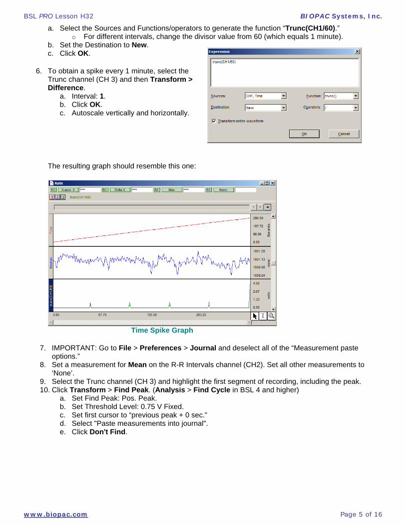
a. Select the Sources and Functions/operators to generate the function “Trunc(CH1/60).” o For different intervals, change the divisor value from 60 (which equals 1 minute).

b. Set the Destination to New. c. Click OK.

6. To obtain a spike every 1 minute, select the Trunc channel (CH 3) and then Transform > Difference.

a. Interval: 1. b. Click OK. c. Autoscale vertically and horizontally.

The resulting graph should resemble this one:

Time Spike Graph

7. IMPORTANT: Go to File > Preferences > Journal and deselect all of the “Measurement paste options.”

8. Set a measurement for Mean on the R-R Intervals channel (CH2). Set all other measurements to ‘None’.

9. Select the Trunc channel (CH 3) and highlight the first segment of recording, including the peak. 10. Click Transform > Find Peak. (Analysis > Find Cycle in BSL 4 and higher)

a. Set Find Peak: Pos. Peak. b. Set Threshold Level: 0.75 V Fixed. c. Set first cursor to “previous peak + 0 sec.” d. Select "Paste measurements into journal". e. Click Don't Find.



Above: Find Peak setup dialog (BSL 3.7x)

Above: Find Cycle setup tabs and dialogs (BSL 4)

11. Show the Journal by clicking on the ‘Journal’ toolbar button. 12. Move the cursor to the left of the first peak and choose Transform > Find All Peaks. (Analysis >

Find All Cycles in BSL 4 and higher. In BSL 4, choose the Output tab to set Paste option).

You should now have the measurements pasted into the journal:



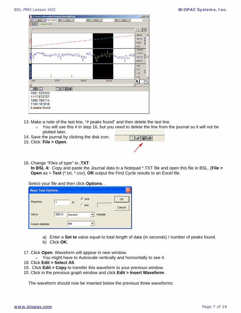
13. Make a note of the last line, “# peaks found” and then delete the last line. o You will use this # in step 16, but you need to delete the line from the journal so it will not be

plotted later. 14. Save the journal by clicking the disk icon. 15. Click: File > Open.

16. Change “Files of type” to .TXT. In BSL 4: Copy and paste the Journal data to a Notepad *.TXT file and open this file in BSL. (File > Open as > Text (*.txt, *.csv), OR output the Find Cycle results to an Excel file.

Select your file and then click Options. .

a) Enter a Set to value equal to total length of data (in seconds) / number of peaks found. b) Click OK.

17. Click Open. Waveform will appear in new window. o You might have to Autoscale vertically and horizontally to see it.

18. Click Edit > Select All. 19. Click Edit > Copy to transfer this waveform to your previous window. 20. Click in the previous graph window and click Edit > Insert Waveform.

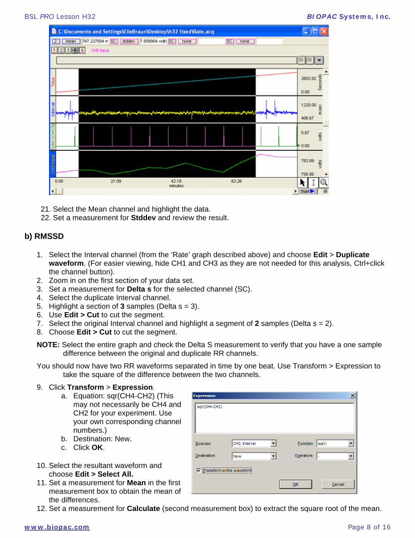
The waveform should now be inserted below the previous three waveforms:



21. Select the Mean channel and highlight the data. 22. Set a measurement for Stddev and review the result.

b) RMSSD

1. Select the Interval channel (from the ‘Rate’ graph described above) and choose Edit > Duplicate waveform. (For easier viewing, hide CH1 and CH3 as they are not needed for this analysis, Ctrl+click the channel button).

2. Zoom in on the first section of your data set. 3. Set a measurement for Delta s for the selected channel (SC). 4. Select the duplicate Interval channel. 5. Highlight a section of 3 samples (Delta s = 3). 6. Use Edit > Cut to cut the segment. 7. Select the original Interval channel and highlight a segment of 2 samples (Delta s = 2). 8. Choose Edit > Cut to cut the segment.

NOTE: Select the entire graph and check the Delta S measurement to verify that you have a one sample difference between the original and duplicate RR channels.

You should now have two RR waveforms separated in time by one beat. Use Transform > Expression to take the square of the difference between the two channels.

9. Click Transform > Expression. a. Equation: sqr(CH4-CH2) (This

may not necessarily be CH4 and CH2 for your experiment. Use your own corresponding channel numbers.)

b. Destination: New. c. Click OK.

10. Select the resultant waveform and choose Edit > Select All.

11. Set a measurement for Mean in the first measurement box to obtain the mean of the differences.

12. Set a measurement for Calculate (second measurement box) to extract the square root of the mean.



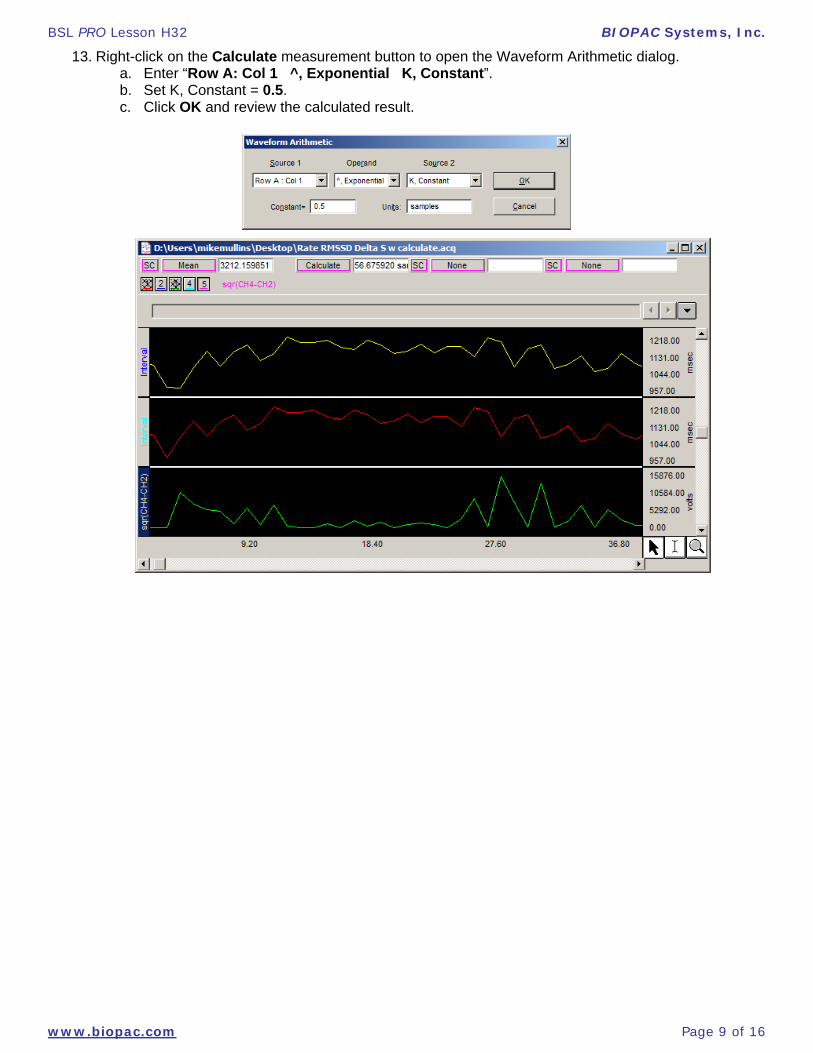
13. Right-click on the Calculate measurement button to open the Waveform Arithmetic dialog. a. Enter “Row A: Col 1 ^, Exponential K, Constant”. b. Set K, Constant = 0.5. c. Click OK and review the calculated result.



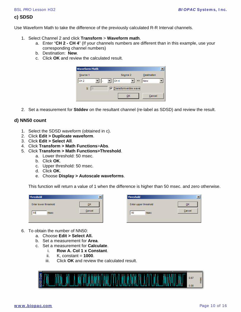
c) SDSD

Use Waveform Math to take the difference of the previously calculated R-R Interval channels.

1. Select Channel 2 and click Transform > Waveform math. a. Enter “CH 2 - CH 4” (If your channels numbers are different than in this example, use your

corresponding channel numbers) b. Destination: New. c. Click OK and review the calculated result.

2. Set a measurement for Stddev on the resultant channel (re-label as SDSD) and review the result.

d) NN50 count

1. Select the SDSD waveform (obtained in c). 2. Click Edit > Duplicate waveform. 3. Click Edit > Select All. 4. Click Transform > Math Functions>Abs. 5. Click Transform > Math Functions>Threshold.

a. Lower threshold: 50 msec. b. Click OK. c. Upper threshold: 50 msec. d. Click OK. e. Choose Display > Autoscale waveforms.

This function will return a value of 1 when the difference is higher than 50 msec. and zero otherwise.

6. To obtain the number of NN50: a. Choose Edit > Select All. b. Set a measurement for Area. c. Set a measurement for Calculate.

i. Row A. Col 1 x Constant. ii. K, constant = 1000. iii. Click OK and review the calculated result.



e) PNN50

Each beat corresponds to one point or one sample, so you can obtain a percentage by taking the NN50 Count and dividing it by the number of samples, and then multiplying by 100.

1. Set a measurement to samples. 2. Set a measurement to Calculate.

a. K / Row (Samples). b. K = NN50 count (as determined in Step D6). c. Click OK and review the calculated result.

3. Manually multiply the result by 100 to get a percentage.

Geometric measures

Geometric measures are most applicable to long term recordings (24 hours preferred), where the histogram follows a normal distribution. A brief theoretical explanation of two geometrical measures follows, but the user is encouraged to conduct further research on the measures, beginning with the comprehensive overview provided in Guidelines: Heart Rate Variability, European Heart Journal (1996) 17, 354-381.

a) HRV triangular index:

Using a discrete scale, the measurement is approximated by:

(Total number of NN intervals) / (Height of the histogram of all NN intervals as measured on a discrete scale)

1. From the raw ECG waveform, click Transform > Find Rate. (Analysis > Find Rate in BSL 4 and higher).

a. Function: Interval: Sec. b. Click to put result in a new graph.

2. Change the display to Chart mode. 3. Autoscale the result horizontally. 4. Select the R-R Interval channel. 5. To convert R-R Interval from seconds to msec, click Transform > Waveform Math.

a. Enter "CH2 x K, Constant" b. Set K, Constant = 1000. c. Click OK. d. Double-click on 'seconds' on the vertical scale bar of the waveform. e. In the dialog box, change the units from seconds to milliseconds (or msec). f. Click OK.

6. Select the first few data points (which are artifacts) and choose Edit > Cut. 7. Set a measurement for P-P. 8. Set a measurement for Calculate.

a. Enter "Row (P-P) / K, Constant." b. Set K, Constant = 7.8125

NOTE: Most experience has been obtained using bin lengths of approximately 8 ms (precisely 7.8125 ms = 1/128 seconds) which corresponds to the precision of the current commercial equipment.

c. Set units to “msec”. This gives you an approximation of the number of bins to use.

9. Set a measurement to Samples and choose Edit > Select All to determine the total number of points.


http://www.escardio.org/guidelines-surveys/esc-guidelines/Scientific_Statements/Documents/guidelines-Heart-Rate-Variability-FT-1996.pdf


10. Click Transform > Histogram. a. For the bins value, enter the Calculate

result yielded in Step 8. b. Select Autorange. c. Click OK.

11. Click on the histogram and choose Edit > Select All.

12. Set a measurement to max. 13. Set a measurement to calculate. 14. Enter “K, Constant / Row (max)”. 15. Set K, Constant = total number of samples (as

determined by the Samples measurement in Step 9). 16. Click OK and review the calculated result.

Measure the height of the Histogram. That is the HRV index.

In this example, 268 samples were taken; the number of

hits in the modal bin was 17 and the triangular index is 15.765.

b) TINN Triangular interpolation of NN

This measurement provides the baseline width of the distribution measured as a base of a triangle, approximating the NN interval distribution HRV.

1. Select the Histogram. 2. Set a measurement for Delta X. 3. Highlight the area between the point of initial increase on the bell curve distribution and the point of end

of decline (return to baseline). 4. Review the Delta X result.



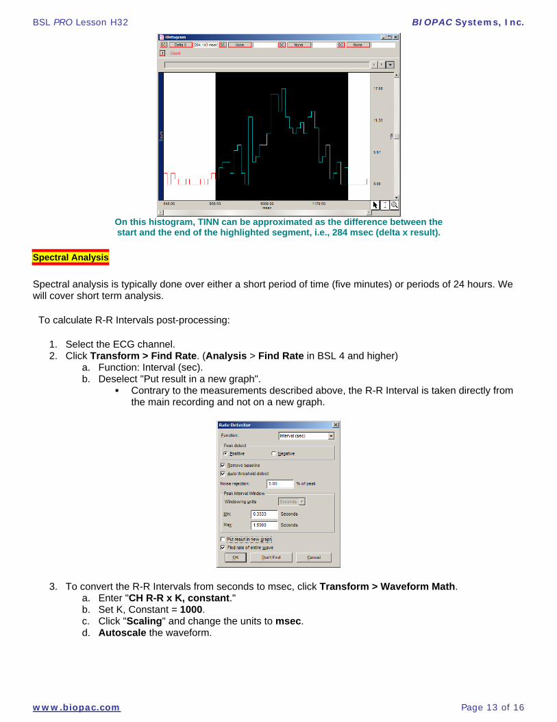
On this histogram, TINN can be approximated as the difference between the start and the end of the highlighted segment, i.e., 284 msec (delta x result).

Spectral Analysis

Spectral analysis is typically done over either a short period of time (five minutes) or periods of 24 hours. We will cover short term analysis.

To calculate R-R Intervals post-processing:

1. Select the ECG channel. 2. Click Transform > Find Rate. (Analysis > Find Rate in BSL 4 and higher)

a. Function: Interval (sec). b. Deselect "Put result in a new graph".

Contrary to the measurements described above, the R-R Interval is taken directly from the main recording and not on a new graph.

3. To convert the R-R Intervals from seconds to msec, click Transform > Waveform Math. a. Enter "CH R-R x K, constant." b. Set K, Constant = 1000. c. Click "Scaling" and change the units to msec. d. Autoscale the waveform.



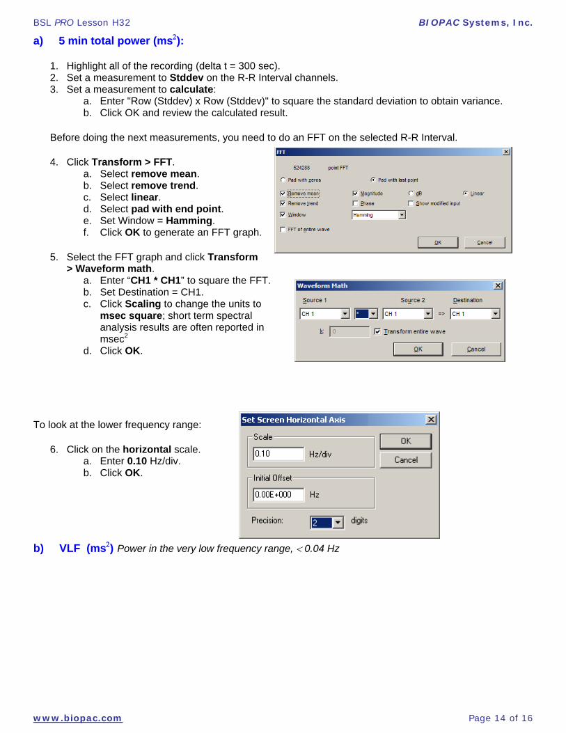
a) 5 min total power (ms):

1. Highlight all of the recording (delta t = 300 sec). 2. Set a measurement to Stddev on the R-R Interval channels. 3. Set a measurement to calculate:

a. Enter "Row (Stddev) x Row (Stddev)" to square the standard deviation to obtain variance. b. Click OK and review the calculated result.

Before doing the next measurements, you need to do an FFT on the selected R-R Interval.

4. Click Transform > FFT. a. Select remove mean. b. Select remove trend. c. Select linear. d. Select pad with end point. e. Set Window = Hamming. f. Click OK to generate an FFT graph.

5. Select the FFT graph and click Transform > Waveform math.

a. Enter “CH1 * CH1” to square the FFT. b. Set Destination = CH1. c. Click Scaling to change the units to

msec square; short term spectral analysis results are often reported in msec2

d. Click OK.

To look at the lower frequency range:

6. Click on the horizontal scale. a. Enter 0.10 Hz/div. b. Click OK.

b) VLF (ms) Power in the very low frequency range, 0.04 Hz



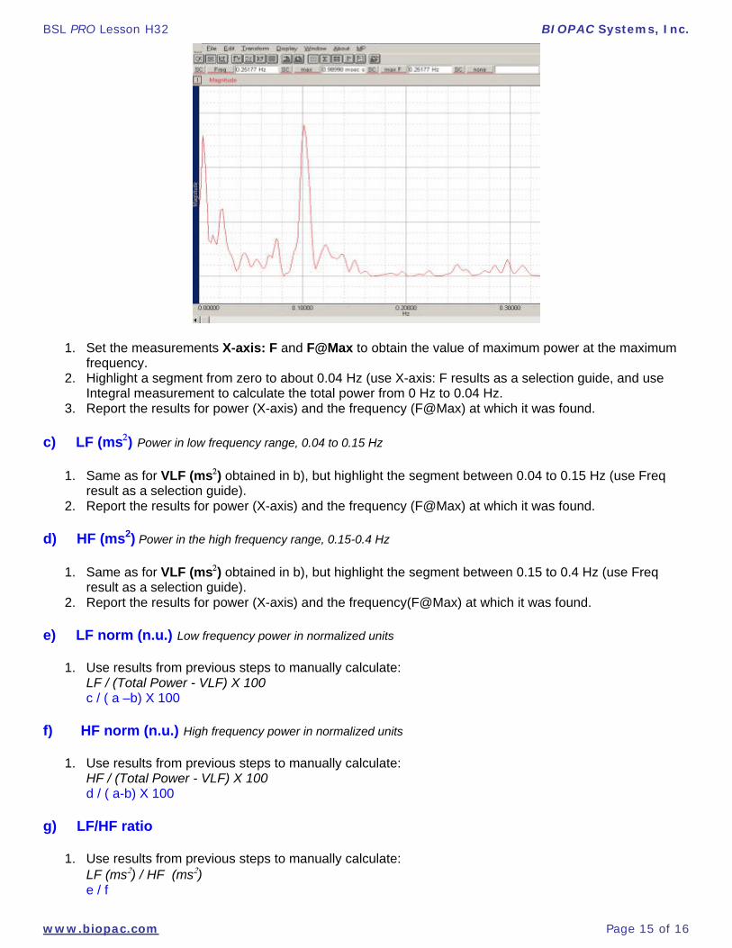
1. Set the measurements X-axis: F and F@Max to obtain the value of maximum power at the maximum frequency.

2. Highlight a segment from zero to about 0.04 Hz (use X-axis: F results as a selection guide, and use Integral measurement to calculate the total power from 0 Hz to 0.04 Hz.

3. Report the results for power (X-axis) and the frequency (F@Max) at which it was found.

c) LF (ms) Power in low frequency range, 0.04 to 0.15 Hz

1. Same as for VLF (ms) obtained in b), but highlight the segment between 0.04 to 0.15 Hz (use Freq result as a selection guide).

2. Report the results for power (X-axis) and the frequency (F@Max) at which it was found.

d) HF (ms2) Power in the high frequency range, 0.15-0.4 Hz

1. Same as for VLF (ms) obtained in b), but highlight the segment between 0.15 to 0.4 Hz (use Freq result as a selection guide).

2. Report the results for power (X-axis) and the frequency(F@Max) at which it was found.

e) LF norm (n.u.) Low frequency power in normalized units

1. Use results from previous steps to manually calculate: LF / (Total Power - VLF) X 100 c / ( a –b) X 100

f) HF norm (n.u.) High frequency power in normalized units

1. Use results from previous steps to manually calculate: HF / (Total Power - VLF) X 100 d / ( a-b) X 100

g) LF/HF ratio

1. Use results from previous steps to manually calculate: LF (ms) / HF (ms) e / f



www.biopac.com

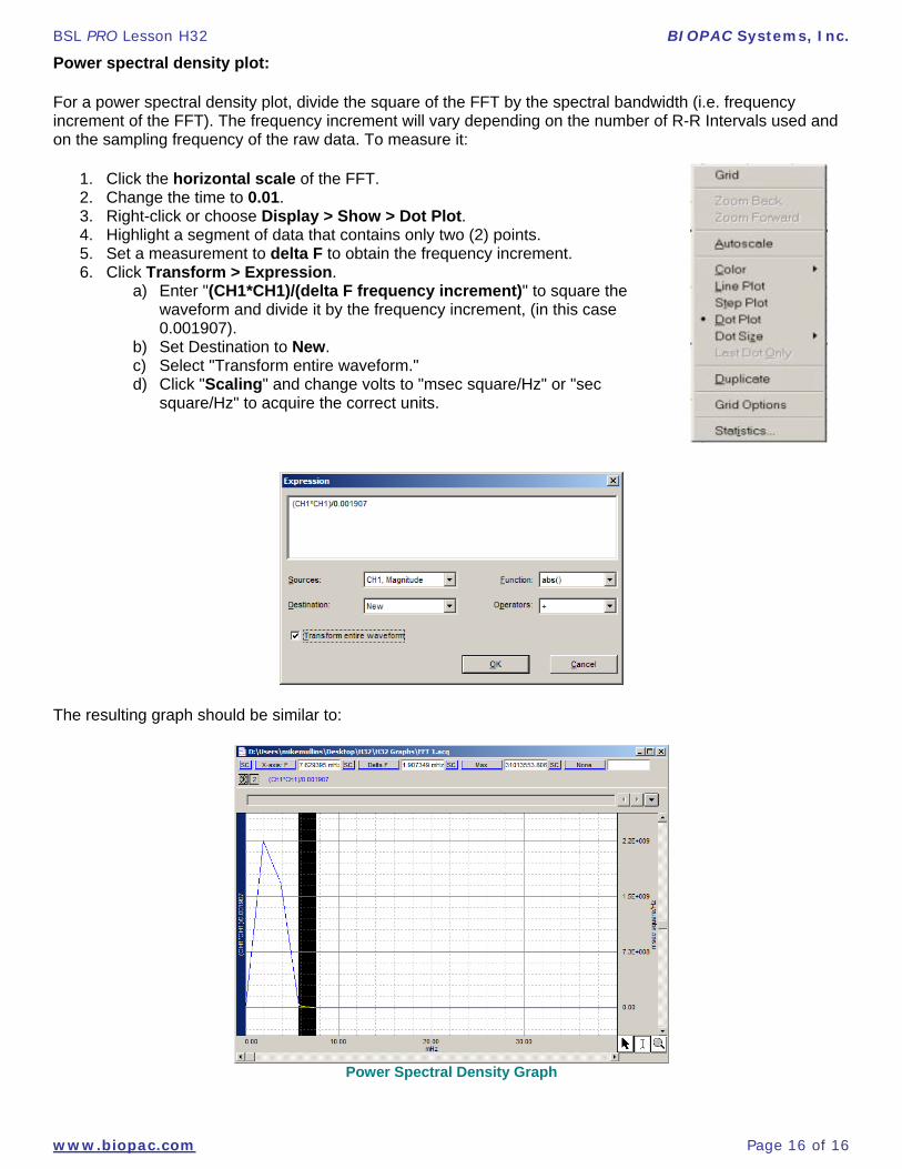
Power spectral density plot:

For a power spectral density plot, divide the square of the FFT by the spectral bandwidth (i.e. frequency increment of the FFT). The frequency increment will vary depending on the number of R-R Intervals used and on the sampling frequency of the raw data. To measure it:

1. Click the horizontal scale of the FFT. 2. Change the time to 0.01. 3. Right-click or choose Display > Show > Dot Plot. 4. Highlight a segment of data that contains only two (2) points. 5. Set a measurement to delta F to obtain the frequency increment. 6. Click Transform > Expression.

a) Enter "(CH1*CH1)/(delta F frequency increment)" to square the waveform and divide it by the frequency increment, (in this case 0.001907).

b) Set Destination to New. c) Select "Transform entire waveform." d) Click "Scaling" and change volts to "msec square/Hz" or "sec

square/Hz" to acquire the correct units.

The resulting graph should be similar to:

Power Spectral Density Graph

Page 16 of 16