Embed Size (px)
Citation preview

0278-0046 (c) 2018 IEEE. Personal use is permitted, but republication/redistribution requires IEEE permission. See http://www.ieee.org/publications_standards/publications/rights/index.html for more information.
This article has been accepted for publication in a future issue of this journal, but has not been fully edited. Content may change prior to final publication. Citation information: DOI 10.1109/TIE.2018.2890506, IEEETransactions on Industrial Electronics
IEEE TRANSACTIONS ON INDUSTRIAL ELECTRONICS
Abstract—3D color laser ranging technology plays a crucial role in many applications. This paper develops a new omnidirectional 3D color laser ranging system. It consists of a 2D laser rangefinder (LRF), a color camera, and a rotating platform. Both the 2D LRF and the camera rotate with the rotating platform to collect line point clouds and images synchronously. The line point clouds and the images are then fused into a 3D color point cloud by a novel calibration method of a 2D LRF and a camera based on an improved checkerboard pattern with rectangle holes. In the calibration, boundary constraint and mean approximation are deployed to accurately compute the centers of rectangle holes from the raw sensor data based on data correction. Then, the data association between the 2D LRF and the camera is directly established to determine their geometric mapping relationship. These steps make the calibration process simple, accurate, and reliable. The experiments show that the proposed calibration method is accurate, robust to noise, and suitable for different geometric structures, and the developed 3D color laser ranging system has good performance for both indoor and outdoor scenes.
Index Terms—Camera calibration, color point cloud,
data fusion, extrinsic calibration, laser rangefinder.
I. INTRODUCTION
ODAY, 3D color laser ranging technology has gradually
been used in digitizing the real world for many application
domains, such as autonomous navigation, object identification,
and industrial inspection. This technology uses a camera and a
laser rangefinder (LRF) to collect 2D images and 3D point
clouds respectively, and then fuses them into 3D color point
clouds to record both geometry and color information of objects
Manuscript received August 20, 2018; revised October 28, 2018;
accepted December 14, 2018. This work was supported in part by the National Natural Science Foundation of China under Grant 61673083, in part by the Natural Science Foundation of Liaoning Province under Grant 20170540167, and in part by the Fundamental Research Funds for the Central Universities under Grant DUT17LAB01.
Y. An, B. Li, and X. Zhou are with the School of Control Science and Engineering, Dalian University of Technology, Dalian 116023, China (e-mail: [email protected]; [email protected]; zhouxiaoli [email protected]).
H. Hu is with the School of Computer Science and Electronic Engineering, University of Essex, Colchester CO4 3SQ, U.K. (e-mail: [email protected]).
and describe the world realistically. The 2D image and 3D point
cloud of an object belong to different modes. They are collected
by different devices and express different aspects of meanings
of the object. Thus, the fusion of 3D point clouds and images is
multimodal data fusion, which is different from multiset data
fusion where the data are the same type of measurement taken
at different time or places [1], [2].
Since LRFs and cameras have different mechanisms, their
synchronization is a challenge. Most existing 3D color laser
ranging systems collect 3D point clouds first and 2D images
subsequently. They are suitable for static scenes and can't work
in dynamic scenes. Therefore, how to achieve the accurate
synchronization of 3D color laser ranging systems is required to
be further investigated.
After data collection, 3D laser point clouds and 2D images
are fused into 3D color point clouds by the geometric mapping
relationship (perspective projection) between the LRF and the
camera, which is determined by the calibration of the LRF and
the camera. Each 3D laser point is colored by its corresponding
pixel in the 2D image. This geometric mapping relationship
includes intrinsic parameters, such as focal length, scale factor,
and principal point, and extrinsic parameters, such as rotation
matrix and translation vector between the LRF and the camera.
In general, the calibration of a LRF and a camera takes three
steps: 1) the intrinsic parameters are computed by the camera
calibration; 2) the extrinsic parameters are obtained by the
extrinsic calibration; 3) the geometric mapping relationship is
calculated by using the intrinsic and extrinsic parameters. In
this process, the calibration data (geometric elements, such as
points, lines, and planes [3]) are obtained from raw sensor data
and used for constructing geometric constraints to solve the
intrinsic and extrinsic parameters. The accurate and abundant
calibration data will lead to a good calibration result. Thus, how
to improve the accuracy of calibration data is a key problem to
be addressed, which is not completely resolved so far [4].
In addition, the three-step calibration process is relatively
complicated. In most application cases, the values for the
intrinsic and extrinsic parameters are useless in themselves,
since only the geometric mapping relationship between a LRF
and a camera is required. Therefore, the simplest strategy to
perform the calibration of a LRF and a camera is to directly
establish some kind of data association between the two sensors
to compute their geometric mapping relationship.
This paper presents a new omnidirectional 3D color laser
Building an Omnidirectional 3D Color Laser Ranging System through a Novel Calibration
Method
Yi An, Member, IEEE, Bo Li, Huosheng Hu, Senior Member, IEEE, and Xiaoli Zhou
T
0278-0046 (c) 2018 IEEE. Personal use is permitted, but republication/redistribution requires IEEE permission. See http://www.ieee.org/publications_standards/publications/rights/index.html for more information.
This article has been accepted for publication in a future issue of this journal, but has not been fully edited. Content may change prior to final publication. Citation information: DOI 10.1109/TIE.2018.2890506, IEEETransactions on Industrial Electronics
IEEE TRANSACTIONS ON INDUSTRIAL ELECTRONICS
ranging system for the generation of 3D color point cloud data.
Two sensors, a 2D LRF and a camera, rotate with a rotating
platform to collect line point clouds and images synchronously.
The software and hardware are developed to ensure the
accurate synchronization. The collected data are then fused into
a color point cloud by a novel calibration method of a 2D LRF
and a camera based on a specially designed calibration board.
During the calibration, line fitting and intersection calculation
are conducted to reduce the noise. Both boundary constraint
and mean approximation are deployed to accurately compute
the geometric elements from the raw sensor data. Then, the data
association between the 2D LRF and the camera is directly
established to determine their geometric mapping relationship.
In this paper, scalars are represented by italic symbols, e.g. 𝑥;
vectors are denoted by bold italic symbols, e.g. 𝒑; sets, matrices,
and intervals are indicated by italic capital symbols, e.g. 𝑃, 𝐻,
and 𝐼; geometric entities (holes, boundaries, and lines) are also
represented by italic symbols, e.g. ℎ, 𝑏, and 𝑙. The rest of the paper is organized as follows. Section II
reviews the previous work related to this research. The 3D color
laser ranging system is described in Section III. In Section IV,
our calibration method is detailed. Experimental results are
presented in Section V to show the performance of our system.
Finally, a conclusion and future work are given in Section VI.
I. RELATED WORK
A. Camera Calibration
Camera calibration is the process of determining the internal
geometric and optical characteristics of a camera (intrinsic
parameters) and/or the position and orientation of a camera
relative to a world coordinate system (extrinsic parameters) by
only using 2D images from the camera [5].
Abdel-Aziz and Karara [6] developed a classic direct linear
transformation (DLT) method to perform camera calibration.
However, a singularity will be introduced in the least squares
fashion with a constraint. In order to improve the numerical
stability, Faugeras and Toscani [7] suggested another new
constraint that is singularity free. Based on the DLT method,
Melen [8] proposed an approach to extract the intrinsic and
extrinsic parameters from the DLT matrix by using the RQ
decomposition. Heikkila and Silven [9] extended the DLT
method to a four-step camera calibration procedure. The most
popular camera calibration method was proposed by Zhang
[10]. It requires a camera to observe a planar pattern at different
poses. Later, he also proposed another camera calibration
technique based on 1D calibration objects [11]. Recently, Font
comas et al. [5] presented a camera calibration methodology by
using a checkerboard pattern for a passive imaging system.
B. Extrinsic Calibration of a LRF and a Camera
Extrinsic calibration of a LRF and a camera is the process of
determining their relative position and orientation (extrinsic
parameters) by using both sensor data (3D point clouds and 2D
images) [12]. The extrinsic calibration methods are divided into
two kinds according to the type of LRF, i.e. 3D or 2D LRF.
1) Extrinsic Calibration of a 3D LRF and a Camera
The 3D LRF uses the area scan technique to acquire a set of
discrete points on object surfaces, namely the area point cloud.
Rushmeier et al. [13] used a cube with checkerboard patterns to
construct plane-to-plane constraints for the extrinsic calibration.
Sergio et al. [14] presented an extrinsic calibration method
based on point-to-point constraints by scanning a circle-based
calibration object. Geiger et al. [15] developed an automatic
calibration method based on plane-to-plane and point-to-plane
constraints by observing a specific scenario. Gong et al. [16]
calibrated a 3D LRF and a camera extrinsically based on the
geometric constraints associated with an arbitrary trihedron.
Recently, Zhuang et al. [17] deployed a checkerboard pattern
with round holes for automatic extrinsic calibration. Walch and
Eitzinger [18] proposed a novel calibration method of a laser
sensor and a camera based on point correspondences.
2) Extrinsic Calibration of a 2D LRF and a Camera
The 2D LRF uses the line scan technique to acquire a series
of discrete points on the intersecting line of the scan plane and
object surfaces, namely the line point cloud. Zhang and Pless
[19] proposed a classical method based on point-to-plane
constraints by using a checkerboard pattern for the extrinsic
calibration of a 2D LRF and a camera. Vasconcelos et al. [20]
presented an extrinsic calibration algorithm by freely moving a
checkerboard pattern, which is formulated as one of registering
a set of lines and planes in the dual 3D space. However, it
suffered from numerical instability. Instead of the dual 3D
space, Ying et al. [4] proposed a direct approach in the 3D
space by using a checkerboard pattern. In order to improve
numerical stability, Zhou [3] exploited the algebraic structure
of the polynomial system to present a new minimal solution for
the extrinsic calibration based on 3 plane-line correspondences.
Apart from checkerboard patterns, an orthogonal trihedron is
also used as the calibration object to simply calibration process.
Gomez-Ojeda et al. [21] presented the first method that only
required the observation of an orthogonal trihedron commonly
found from a scene corner in most environments. Briales and
Gonzalez-Jimenez [22] also proposed a minimal solution for
the extrinsic calibration by using a scene corner. Hu et al. [23]
calibrated a 2D LRF and a camera extrinsically by observing an
orthogonal trihedron based on point-to-point constraints.
C. Discussion
In all the above-mentioned extrinsic calibration methods of a
2D LRF and a camera, the pose of the calibration object in the
camera coordinate system need to be determined in advance by
another camera calibration. This additional camera calibration
process is a prerequisite for constructing geometric constraints
to solve the extrinsic parameters between a 2D LRF and a
camera, which in turn makes extrinsic calibration complex.
And, the camera calibration error could affect the performance
of the extrinsic calibration of a 2D LRF and a camera [19].
In fact, camera calibration or extrinsic calibration is only a
step in the common three-step calibration process of a 2D LRF
and a camera, which is relatively complicated. To simplify such
a calibration, we could directly establish some kind of data
0278-0046 (c) 2018 IEEE. Personal use is permitted, but republication/redistribution requires IEEE permission. See http://www.ieee.org/publications_standards/publications/rights/index.html for more information.
This article has been accepted for publication in a future issue of this journal, but has not been fully edited. Content may change prior to final publication. Citation information: DOI 10.1109/TIE.2018.2890506, IEEETransactions on Industrial Electronics
IEEE TRANSACTIONS ON INDUSTRIAL ELECTRONICS
association between the two sensors to compute their geometric
mapping relationship. This has inspired us to conduct our
research in this paper. In addition, as the computation of the
geometric elements from the raw sensor data determines the
calibration accuracy, we pay close attention to the computation
of geometric elements, especially from the 2D LRF data. The
technique comparison between conventional methods and the
proposed method is shown in Table I.
II. 3D COLOR LASER RANGING SYSTEM
A. System Design and Working Principle
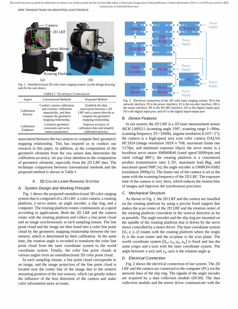
Fig. 1 shows the proposed omnidirectional 3D color ranging
system that is composed of a 2D LRF, a color camera, a rotating
platform, a servo motor, an angle encoder, a slip ring, and a
computer. The rotating platform rotates continuously at a speed
according to applications. Both the 2D LRF and the camera
rotate with the rotating platform and collect a line point cloud
and an image synchronously at each sampling instant. The line
point cloud and the image are then fused into a color line point
cloud by the geometric mapping relationship between the two
sensors, which is determined by their calibration. At the same
time, the rotation angle is recorded to transform the color line
point cloud from the laser coordinate system to the world
coordinate system. Finally, the color line point clouds at
various angles form an omnidirectional 3D color point cloud.
At each sampling instant, a line point cloud corresponds to
an image, and the image projection of the line point cloud is
located near the center line of the image due to the relative
mounting position of the two sensors, which can greatly reduce
the influence of the lens distortion of the camera and make
color information more accurate.
B. Device Features
In our system, the 2D LRF is a 2D laser measurement sensor
SICK LMS511 (scanning angle 190°, scanning range 1~80m,
scanning frequency 25~100Hz, angular resolution 0.167~1°);
the camera is a high-speed area scan color camera DALSA
HC1024 (image resolution 1024 × 768, maximum frame rate
117fps, and minimum exposure 10𝜇s); the servo motor is a
brushless servo motor SM060R40 (rated speed 3000rpm and
rated voltage 48V ); the rotating platform is a customized
product (transmission ratio 1: 20 , maximum load 8kg , and
maximum speed 900°/s); the angle encoder is OMRON-E6B2
(resolution 2000p/r). The frame rate of the camera is set as the
same with the scanning frequency of the 2D LRF. The exposure
time of the camera is very short, which reduces the motion blur
of images and improves the synchronous precision.
C. Mechanical Structure
As shown in Fig. 1, the 2D LRF and the camera are installed
on the rotating platform by using a precise fixed support that
makes the scan center of the 2D LRF and the rotation center of
the rotating platform coincident in the vertical direction as far
as possible. The angle encoder and the slip ring are mounted on
the spindle of the rotating platform that is driven by the servo
motor controlled by a motor driver. The laser coordinate system
[𝑂𝑙; 𝑥, 𝑦, 𝑧] rotates with the rotating platform where the origin
𝑂𝑙 is the scan center and the 𝑥𝑧-plane is the scan plane. The
world coordinate system [𝑂𝑤; 𝑥𝑤 , 𝑦𝑤 , 𝑧𝑤] is fixed and has the
same origin and 𝑧-axis with the laser coordinate system. The
angle between 𝑥-axis and 𝑥𝑤-axis is the rotation angle 𝜑.
D. Electrical Connection
Fig. 2 shows the electrical connection of our system. The 2D
LRF and the camera are connected to the computer (PC) via the
network lines of the slip ring. The signals of the angle encoder
are acquired by a data collection module (DCM). The data
collection module and the motor driver communicate with the
Camera
2D LRF
Servo Motor
Rotating Platform
yw
x xwy
z zw
j
(a) (b)
Fig. 1. Omnidirectional 3D color laser ranging system: (a) the design drawing
and (b) the real object.
Slip
Ring
NI-1
NI-2
I/O
NI-1
NI-2
PI-1
PI-2
I/O
Power
Supply
PI-1
PI-22D LRF
PI
NIDO
Power
Supply
Power
Supply
Power
Supply
Power
Supply
CameraPI
NI
DISwitch
NI-3
PINI-1
NI-2
Angle
EncoderEI
Servo
MotorMI
DCM PI
DI
RS
Motor
Driver PI
RSMI
PCPI
NIRS
EI
DI
DO
DO
Fig. 2. Electrical connection of the 3D color laser ranging system. NI is the
network interface, PI is the power interface, EI is the encoder interface, MI is the motor interface, RS is the RS-485 interface, DO is the digital output port,
DI is the digital input port, and I/O is the digital input/output port.
TABLE I TECHNIQUE COMPARISON
Aspect Conventional Methods Proposed Method
Calibration Process
Conduct camera calibration and extrinsic calibration
sequentially, and then
compute the geometric mapping relationship.
Establish the data association between a 2D
LRF and a camera directly to
compute the geometric mapping relationship.
Calibration Emphasis
Construct geometric
constraints and solve
camera parameters.
Improve accuracy of
calibration data and simplify
calibration process.

0278-0046 (c) 2018 IEEE. Personal use is permitted, but republication/redistribution requires IEEE permission. See http://www.ieee.org/publications_standards/publications/rights/index.html for more information.
This article has been accepted for publication in a future issue of this journal, but has not been fully edited. Content may change prior to final publication. Citation information: DOI 10.1109/TIE.2018.2890506, IEEETransactions on Industrial Electronics
IEEE TRANSACTIONS ON INDUSTRIAL ELECTRONICS
computer by a RS-485 serial bus. For data synchronization, the
digital output port (DO) of the computer is connected to the
digital input ports (DI) of the data collection module and the
camera via the signal line of the slip ring.
E. Synchronous Data Collection
The computer software sends the data collection command to
the 2D LRF. When receiving the command, the 2D LRF starts
to scan the scene and send the scan data to the computer at the
scanning frequency. Each frame of scan data includes a line
point cloud and a timestamp. The timestamp of the 2D LRF is
accurate and stable, and can be used as the reference time. It is
initialized according to the time of the computer. And then, the
computer sets the synchronous triggering time in accord with
the timestamp beforehand and send a high-level synchronous
collection signal to both the camera and the data collection
module via the hardware digital I/O ports at the triggering time.
This signal simultaneously triggers the camera to take the
image of the scene and the data collection module to record the
rotation angle. The cooperation of the software command and
hardware signal guarantees that the line point cloud, image, and
rotation angle are collected synchronously as far as possible.
F. Rotation Angle Processing
Without loss of generality, we can assume that the scanning
frequency, scanning angle, and angular resolution of the 2D
LRF are set to 100Hz, 180°, and 0.25° respectively. Therefore,
the time to conduct a scan is about 1/100Hz = 10ms, and each
scan (line point cloud) has 180°/0.25° = 720 laser points. If
the rotate speed 𝜔 of the rotating platform is set as 180°/s, the
rotating platform turns 180°/s × 10ms = 1.8° within a scan.
Then, the rotating angle difference ∆𝜑 between two adjacent
laser points is 1.8°/720 = 0.0025°. When 𝜔 ≤ 180°/s, since
∆𝜑 is very small, the rotation angle 𝜑𝑖 of each laser point in a
scan can be set to the rotation angle 𝜑, which is acquired by
synchronous data collection with the angle encoder at the same
sampling instant; when 𝜔 > 180°/s, since ∆𝜑 is slightly larger,
we can use an angle compensation mechanism to improve the
accuracy of the rotation angle as follows: 𝜑𝑖 = 𝜑 + (𝑖 − 1)∆𝜑,
where 𝜑𝑖 is the rotation angle of the 𝑖th laser point in a scan and
∆𝜑 = 𝜔/(100 × 720) . For other scanning frequencies and
rotate speeds, we can use the similar mechanism to improve the
accuracy of the rotation angle and reduce their effects.
III. MULTIMODAL DATA FUSION
A. Novel Calibration Board
Fig. 3 shows our calibration board for the calibration of a 2D
LRF and a camera, which is an improved checkerboard pattern.
Its novelty lies in the design of a narrow rectangle hole centered
on each corner in the center line of the calibration board. The
size of the narrow rectangle is 2cm × 6cm. Its length 𝑙 = 6cm
is half size of the side length of the checkerboard square 𝑑 =12cm . The calibration board is produced by automatically
printing and mechanically punching to ensure high precision.
The calibration board is placed towards the 2D LRF and the
camera. Its position is adjusted to make the scan plane of the 2D
LRF pass through the centers of the rectangle holes. This can be
achieved by two ways: 1) slowly moving the calibration board
and observing the changing process of the laser points passing
through the rectangle holes to determine the optimal position; 2)
using the white light spots of the laser in the image to determine
the optimal position in the case of no filter installed on the
camera lens. Since the image sensor of the camera is sensitive
to the laser beam of the 2D LRF, we can see the white light
spots of the laser measuring points in the image, which are
actually the image projections of the laser measuring points.
The white light spots of the laser measuring points overlap each
other and compose a thick white line, as shown in Fig. 4(a) and
Fig. 16. The width of the thick white line of the laser is close to
the width of the rectangle hole. Therefore, when the laser beam
passes through the rectangle hole, the center of the laser beam is
very close to the center of the rectangle hole in the horizontal
direction. The horizontal position error is very small and far
less than the laser measurement error (±24mm for LMS511).
For taking a whole scan and image of the calibration board,
the minimum distance between the calibration board and our
system is 1.7m according to the features of the 2D LRF and the
camera. As the distance increases, the number of the laser
points in the line point cloud of the calibration board becomes
less, the measurement noise of the 2D LRF becomes larger, and
the image of the calibration board becomes smaller. All things
considered, the appropriate distance between the calibration
board and the 3D color laser ranging system is 2~4m.
We calibrate the 2D LRF and the camera after they are fixed
tightly on the rotating platform. If the sensors get loose, we
jej
ig
Light Spot
Hole
d
l
(a) (b)
Fig. 4. (a) White light spots of the laser in the image of the calibration board
and (b) computing the center 𝒆𝑗 of the rectangle hole ℎ𝑗 in the image. Calibration Board
3D Color Laser
Ranging System
Scan Plane
Fig. 3. Calibration board and 3D color laser ranging system.
0278-0046 (c) 2018 IEEE. Personal use is permitted, but republication/redistribution requires IEEE permission. See http://www.ieee.org/publications_standards/publications/rights/index.html for more information.
This article has been accepted for publication in a future issue of this journal, but has not been fully edited. Content may change prior to final publication. Citation information: DOI 10.1109/TIE.2018.2890506, IEEETransactions on Industrial Electronics
IEEE TRANSACTIONS ON INDUSTRIAL ELECTRONICS
retighten and recalibrate them to get new geometric mapping.
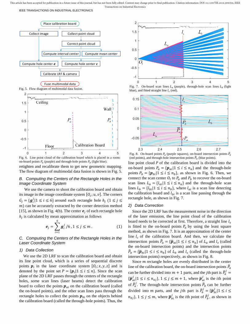
The flow diagram of multimodal data fusion is shown in Fig. 5.
B. Computing the Centers of the Rectangle Holes in the Image Coordinate System
We use the camera to shoot the calibration board and obtain
its image in the image coordinate system [𝑂𝑐; 𝑢, 𝑣]. The corners
𝐺𝑗 = {𝒈𝑖𝑗|1 ≤ 𝑖 ≤ 6} around each rectangle hole ℎ𝑗 (1 ≤ 𝑗 ≤
𝑚) can be accurately extracted by the corner detection method
[15], as shown in Fig. 4(b). The center 𝒆𝑗 of each rectangle hole
ℎ𝑗 is calculated by mean approximation as follows
𝒆𝑗 = ∑ 𝒈𝑖𝑗
6
𝑖=1
/6 , 1 ≤ 𝑗 ≤ 𝑚 . (1)
C. Computing the Centers of the Rectangle Holes in the Laser Coordinate System
1) Data Collection
We use the 2D LRF to scan the calibration board and obtain
its line point cloud, which is a series of sequential discrete
points 𝒑𝑖 in the laser coordinate system [𝑂𝑙; 𝑥, 𝑦, 𝑧] and is
denoted by the point set 𝑃 = {𝒑𝑖|1 ≤ 𝑖 ≤ 𝑛}. Since the scan
plane of the 2D LRF passes through the centers of the rectangle
holes, some scan lines (laser beams) detect the calibration
board to collect the points 𝒑𝑎𝑖 on the calibration board (called
the on-board points), and the other scan lines pass through the
rectangle holes to collect the points 𝒑𝑏𝑖 on the objects behind
the calibration board (called the through-hole points). Thus, the
line point cloud 𝑃 of the calibration board is divided into the
on-board points 𝑃𝑎 = {𝒑𝑎𝑖|1 ≤ 𝑖 ≤ 𝑛𝑎} and the through-hole
points 𝑃𝑏 = {𝒑𝑏𝑖|1 ≤ 𝑖 ≤ 𝑛𝑏}, as shown in Fig. 6. Then, we
connect the scan center 𝑂𝑙 to 𝑃𝑎 and 𝑃𝑏 to recover the on-board
scan lines 𝐿𝑎 = {𝑙𝑎𝑖|1 ≤ 𝑖 ≤ 𝑛𝑎} and the through-hole scan
lines 𝐿𝑏 = {𝑙𝑏𝑖|1 ≤ 𝑖 ≤ 𝑛𝑏}, where 𝑙𝑎𝑖 is a scan line detecting
the calibration board and 𝑙𝑏𝑖 is a scan line passing through the
rectangle hole, as shown in Fig. 7.
2) Data Correction
Since the 2D LRF has the measurement noise in the direction
of the laser emission, the line point cloud of the calibration
board needs to be corrected at first. Therefore, a straight line 𝑙𝑠
is fitted to the on-board points 𝑃𝑎 by using the least square
method, as shown in Fig. 7. It is an approximation of the center
line 𝑙𝑐 of the calibration board. And then, we calculate the
intersection points �̅�𝑎 = {�̅�𝑎𝑖|1 ≤ 𝑖 ≤ 𝑛𝑎} of 𝐿𝑎 and 𝑙𝑠 (called
the on-board intersection points) and the intersection points
�̅�𝑏 = {�̅�𝑏𝑖|1 ≤ 𝑖 ≤ 𝑛𝑏} of 𝐿𝑏 and 𝑙𝑠 (called the through-hole
intersection points) respectively, as shown in Fig. 8.
Since 𝑚 rectangle holes are evenly distributed in the center
line of the calibration board, the on-board intersection points �̅�𝑎
can be further divided into 𝑚 + 1 parts, and the 𝑗th part is �̅�𝑎𝑗
=
{�̅�𝑎𝑖𝑗
|1 ≤ 𝑖 ≤ 𝑛𝑎𝑗}, 1 ≤ 𝑗 ≤ 𝑚 + 1, where �̅�𝑎𝑖𝑗
is the 𝑖th point
of �̅�𝑎𝑗. The through-hole intersection points �̅�𝑏 can be further
divided into 𝑚 parts, and the 𝑗 th part is �̅�𝑏𝑗
= {�̅�𝑏𝑖𝑗
|1 ≤ 𝑖 ≤
𝑛𝑏𝑗}, 1 ≤ 𝑗 ≤ 𝑚, where �̅�𝑏𝑖𝑗
is the 𝑖th point of �̅�𝑏𝑗, as shown in
Fig. 6. Line point cloud of the calibration board which is placed in a room:
on-board points 𝑃𝑎 (purple) and through-hole points 𝑃𝑏 (light blue).
Fig. 7. On-board scan lines 𝐿𝑎 (purple), through-hole scan lines 𝐿𝑏 (light
blue), and fitted straight line 𝑙𝑠 (red).
Fig. 8. On-board points 𝑃𝑎 (purple squares), on-board intersection points �̅�𝑎
(red points), and through-hole intersection points �̅�𝑏 (blue points).
Collect point cloud
Correct point cloud
Place calibration board
Collect image
Compute interval center Compute mean center
Compute hole center e Compute hole center c
Calibrate LRF & camera
Fuse multimodal data
Fig. 5. Flow diagram of multimodal data fusion.
0278-0046 (c) 2018 IEEE. Personal use is permitted, but republication/redistribution requires IEEE permission. See http://www.ieee.org/publications_standards/publications/rights/index.html for more information.
This article has been accepted for publication in a future issue of this journal, but has not been fully edited. Content may change prior to final publication. Citation information: DOI 10.1109/TIE.2018.2890506, IEEETransactions on Industrial Electronics
IEEE TRANSACTIONS ON INDUSTRIAL ELECTRONICS
Fig. 9. The intersection points are the corrected data, which
describe the calibration board and rectangle holes accurately.
This step makes our method robust to the noise.
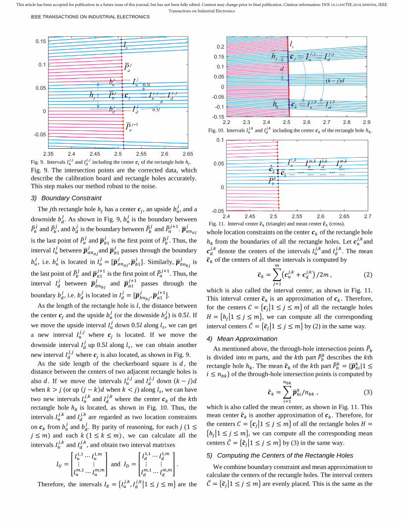
3) Boundary Constraint
The 𝑗th rectangle hole ℎ𝑗 has a center 𝒄𝑗, an upside 𝑏𝑢𝑗, and a
downside 𝑏𝑑𝑗. As shown in Fig. 9, 𝑏𝑢
𝑗 is the boundary between
�̅�𝑎𝑗 and �̅�𝑏
𝑗, and 𝑏𝑑
𝑗 is the boundary between �̅�𝑏
𝑗 and �̅�𝑎
𝑗+1. �̅�𝑎𝑛𝑎𝑗
𝑗
is the last point of �̅�𝑎𝑗 and �̅�𝑏1
𝑗 is the first point of �̅�𝑏
𝑗. Thus, the
interval 𝐼𝑢𝑗 between �̅�𝑎𝑛𝑎𝑗
𝑗and �̅�𝑏1
𝑗 passes through the boundary
𝑏𝑢𝑗, i.e. 𝑏𝑢
𝑗 is located in 𝐼𝑢
𝑗= [�̅�𝑎𝑛𝑎𝑗
𝑗, �̅�𝑏1
𝑗]. Similarly, �̅�𝑏𝑛𝑏𝑗
𝑗 is
the last point of �̅�𝑏𝑗 and �̅�𝑎1
𝑗+1 is the first point of �̅�𝑎
𝑗+1. Thus, the
interval 𝐼𝑑𝑗
between �̅�𝑏𝑛𝑏𝑗
𝑗 and �̅�𝑎1
𝑗+1 passes through the
boundary 𝑏𝑑𝑗, i.e. 𝑏𝑑
𝑗 is located in 𝐼𝑑
𝑗= [�̅�𝑏𝑛𝑏𝑗
𝑗, �̅�𝑎1
𝑗+1].
As the length of the rectangle hole is 𝑙, the distance between
the center 𝒄𝑗 and the upside 𝑏𝑢𝑗 (or the downside 𝑏𝑑
𝑗) is 0.5𝑙. If
we move the upside interval 𝐼𝑢𝑗 down 0.5𝑙 along 𝑙𝑠, we can get
a new interval 𝐼𝑢𝑗,𝑗
where 𝒄𝑗 is located. If we move the
downside interval 𝐼𝑑𝑗 up 0.5𝑙 along 𝑙𝑠 , we can obtain another
new interval 𝐼𝑑𝑗,𝑗
where 𝒄𝑗 is also located, as shown in Fig. 9.
As the side length of the checkerboard square is 𝑑 , the
distance between the centers of two adjacent rectangle holes is
also 𝑑 . If we move the intervals 𝐼𝑢𝑗,𝑗
and 𝐼𝑑𝑗,𝑗
down (𝑘 − 𝑗)𝑑
when 𝑘 > 𝑗 (or up (𝑗 − 𝑘)𝑑 when 𝑘 < 𝑗) along 𝑙𝑠, we can have
two new intervals 𝐼𝑢𝑗,𝑘
and 𝐼𝑑𝑗,𝑘
where the center 𝒄𝑘 of the 𝑘th
rectangle hole ℎ𝑘 is located, as shown in Fig. 10. Thus, the
intervals 𝐼𝑢𝑗,𝑘
and 𝐼𝑑𝑗,𝑘
are regarded as two location constraints
on 𝒄𝑘 from 𝑏𝑢𝑗 and 𝑏𝑑
𝑗. By parity of reasoning, for each 𝑗 (1 ≤
𝑗 ≤ 𝑚) and each 𝑘 (1 ≤ 𝑘 ≤ 𝑚) , we can calculate all the
intervals 𝐼𝑢𝑗,𝑘
and 𝐼𝑑𝑗,𝑘
, and obtain two interval matrixes
𝐼𝑈 = [𝐼𝑢
1,1 ⋯ 𝐼𝑢1,𝑚
⋮ ⋮ 𝐼𝑢
𝑚,1 ⋯ 𝐼𝑢𝑚,𝑚
] and 𝐼𝐷 = [𝐼𝑑
1,1 ⋯ 𝐼𝑑1,𝑚
⋮ ⋮ 𝐼𝑑
𝑚,1 ⋯ 𝐼𝑑𝑚,𝑚
] .
Therefore, the intervals 𝐼𝐾 = {𝐼𝑢𝑗,𝑘
, 𝐼𝑑𝑗,𝑘
|1 ≤ 𝑗 ≤ 𝑚} are the
whole location constraints on the center 𝒄𝑘 of the rectangle hole
ℎ𝑘 from the boundaries of all the rectangle holes. Let 𝒄𝑢𝑗,𝑘
and
𝒄𝑑𝑗,𝑘
denote the centers of the intervals 𝐼𝑢𝑗,𝑘
and 𝐼𝑑𝑗,𝑘
. The mean
�̅�𝑘 of the centers of all these intervals is computed by
�̅�𝑘 = ∑(𝒄𝑢𝑗,𝑘
+ 𝒄𝑑𝑗,𝑘
)
𝑚
𝑗=1
/2𝑚 , (2)
which is also called the interval center, as shown in Fig. 11.
This interval center �̅�𝑘 is an approximation of 𝒄𝑘 . Therefore,
for the centers 𝐶 = {𝒄𝑗|1 ≤ 𝑗 ≤ 𝑚} of all the rectangle holes
𝐻 = {ℎ𝑗|1 ≤ 𝑗 ≤ 𝑚}, we can compute all the corresponding
interval centers 𝐶̅ = {�̅�𝑗|1 ≤ 𝑗 ≤ 𝑚} by (2) in the same way.
4) Mean Approximation
As mentioned above, the through-hole intersection points �̅�𝑏
is divided into 𝑚 parts, and the 𝑘th part �̅�𝑏𝑘 describes the 𝑘th
rectangle hole ℎ𝑘. The mean �̂�𝑘 of the 𝑘th part �̅�𝑏𝑘 = {�̅�𝑏𝑖
𝑘 |1 ≤𝑖 ≤ 𝑛𝑏𝑘} of the through-hole intersection points is computed by
�̂�𝑘 = ∑ �̅�𝑏𝑖𝑘 /𝑛𝑏𝑘
𝑛𝑏𝑘
𝑖=1
, (3)
which is also called the mean center, as shown in Fig. 11. This
mean center �̂�𝑘 is another approximation of 𝒄𝑘. Therefore, for
the centers 𝐶 = {𝒄𝑗|1 ≤ 𝑗 ≤ 𝑚} of all the rectangle holes 𝐻 =
{ℎ𝑗|1 ≤ 𝑗 ≤ 𝑚}, we can compute all the corresponding mean
centers �̂� = {�̂�𝑗|1 ≤ 𝑗 ≤ 𝑚} by (3) in the same way.
5) Computing the Centers of the Rectangle Holes
We combine boundary constraint and mean approximation to
calculate the centers of the rectangle holes. The interval centers
𝐶̅ = {�̅�𝑗|1 ≤ 𝑗 ≤ 𝑚} are evenly placed. This is the same as the
Fig. 11. Interval center �̅�𝑘 (triangle) and mean center �̂�𝑘 (cross).
Fig. 10. Intervals 𝐼𝑢
𝑗,𝑘 and 𝐼𝑑
𝑗,𝑘 including the center 𝒄𝑘 of the rectangle hole ℎ𝑘.
Fig. 9. Intervals 𝐼𝑢
𝑗,𝑗 and 𝐼𝑑
𝑗,𝑗 including the center 𝒄𝑗 of the rectangle hole ℎ𝑗.

0278-0046 (c) 2018 IEEE. Personal use is permitted, but republication/redistribution requires IEEE permission. See http://www.ieee.org/publications_standards/publications/rights/index.html for more information.
This article has been accepted for publication in a future issue of this journal, but has not been fully edited. Content may change prior to final publication. Citation information: DOI 10.1109/TIE.2018.2890506, IEEETransactions on Industrial Electronics
IEEE TRANSACTIONS ON INDUSTRIAL ELECTRONICS
distribution of the centers 𝐶 = {𝒄𝑗|1 ≤ 𝑗 ≤ 𝑚} of the rectangle
holes. Therefore, the interval centers 𝐶̅ can be regarded as an
initial template of the centers 𝐶 of the rectangle holes, which
will be optimized by the mean centers �̂� = {�̂�𝑗|1 ≤ 𝑗 ≤ 𝑚}
along the straight line 𝑙𝑠 via solving the optimal approximation
min ∑‖�̂�𝑗 − (�̅�𝑗 + 𝑡𝒗)‖
𝑚
𝑗=1
, (4)
where 𝒗 is the direction vector of the straight line 𝑙𝑠 and 𝑡 is the
displacement distance of �̅�𝑗 towards �̂�𝑗 along 𝒗. When we get 𝑡,
the center 𝒄𝑗 of each rectangle hole ℎ𝑗 is calculated as
𝒄𝑗 = �̅�𝑗 + 𝑡𝒗, 1 ≤ 𝑗 ≤ 𝑚 . (5)
D. Calibration of the 2D LRF and the Camera
Let 𝒄 = [𝑥, 𝑦, 𝑧]𝑇 denote the center of a rectangle hole in the
laser coordinate system. 𝒆 = [𝑢, 𝑣]𝑇 is its image projection, i.e.
the center of the rectangle hole in the image coordinate system.
Their homogeneous coordinates are �̃� = [𝑥, 𝑦, 𝑧, 1]𝑇 and �̃� =[𝑢, 𝑣, 1]𝑇. By using the pinhole model, the relationship between
the center �̃� of the rectangle hole and its image �̃� is given by
𝑠�̃� = 𝐴[𝑅, 𝒕]�̃� , (6)
where 𝑠 is an arbitrary scale factor, 𝐴 is the intrinsic parameter
matrix, and [𝑅 𝒕] is the extrinsic parameter matrix between the
2D LRF and the camera.
Since the scan plane is the 𝑥𝑧-plane of the laser coordinate
system, we have 𝑦 = 0. Therefore, we can rewrite (6) as
𝑠 [𝑢𝑣1
] = 𝐴[𝒓1 𝒓2 𝒓3 𝒕] [
𝑥0𝑧1
] = 𝐴[𝒓𝟏 𝒓𝟑 𝒕] [𝑥𝑧1
] , (7)
where 𝒓𝑖 is the 𝑖th column vector of the rotation matrix 𝑅 and 𝒕
is the translation vector. �̃� = [𝑥, 0, 𝑧, 1]𝑇 is simplified as �̃� =[𝑥, 𝑧, 1]𝑇. Therefore, the center �̃� of the rectangle hole and its
image �̃� is related by a homography 𝐻 as follows
𝑠�̃� = 𝐻�̃� with 𝐻 = 𝐴[𝒓1 𝒓3 𝒕] , (8)
which directly establishes the data association between the 2D
LRF and the camera. This forms the point-to-point constraint
between the two sensors. Since we have computed multiple
pairs of 𝒆𝑗 and 𝒄𝑗 in Subsection B and C, we can calculate 𝐻 by
solving the nonlinear minimization: min ∑ ‖𝒆𝑗 − �̅�𝑗‖2�̂�
𝑗=1 ,
where 𝒆𝑗 = [𝑢𝑗, 𝑣𝑗]𝑇 and �̅�𝑗 = [𝒉1�̃�𝑗/𝒉3�̃�𝑗 , 𝒉2�̃�𝑗/𝒉3�̃�𝑗]𝑇 , with
the Levenberg-Marquardt method. 𝒉1, 𝒉2, and 𝒉3 are the row
vectors of 𝐻. 𝐻 is the optimal geometric mapping relationship.
E. Data Fusion
At each sampling instant, a line point cloud, an image, and a
rotation angle are collected synchronously. Let 𝒑 = [𝑥, 𝑦, 𝑧]𝑇
be a point in the line point cloud. Its homogeneous coordinate is
�̃� = [𝑥, 𝑦, 𝑧, 1]𝑇 which can be simplified as �̃� = [𝑥, 𝑧, 1]𝑇 since
𝑦 = 0. Its image projection 𝒎 = [𝑢, 𝑣]𝑇 is obtained by
𝑢 = 𝒉1�̃�/𝒉3�̃� and 𝑣 = 𝒉2�̃�/𝒉3�̃� . (9)
Then, we can obtain the color point
𝒑𝑐 = [𝑥, 𝑦, 𝑧, R(𝑢, 𝑣), G(𝑢, 𝑣), B(𝑢, 𝑣)]𝑇 , (10)
where R(𝑢, 𝑣) , G(𝑢, 𝑣) and B(𝑢, 𝑣) denote the three-primary
colors of the image projection 𝒎. Finally, the color point 𝒑𝑐 in
the laser coordinate system is transformed into the color point
𝒑𝑤 = [𝑥𝑤 , 𝑦𝑤 , 𝑧𝑤 , R(𝑢, 𝑣), G(𝑢, 𝑣), B(𝑢, 𝑣)]𝑇 (11)
in the world coordinate system by using the rotation angle 𝜑,
where 𝑥𝑤 = 𝑥𝑐𝑜𝑠𝜑, 𝑦𝑤 = 𝑥𝑠𝑖𝑛𝜑, and 𝑧𝑤 = 𝑧.
IV. EXPERIMENTAL RESULTS
A. Experiments with Synthetic Data
Our calibration method is first evaluated by using synthetic
data that are generated by a simulated 2D LRF and a simulated
camera. The simulated 2D LRF has a 180° scanning angle and
a 0.33° angular resolution. The simulated camera has an 8mm
focal length and an 8.8 × 6.6mm2 imager with a 1024 × 768
array of pixels. For evaluating different methods, two types of
calibration boards are simulated: our improved checkerboard
pattern with rectangle holes and standard checkerboard pattern.
The simulated calibration boards are placed in different poses,
as shown in Fig. 12. Each pose has an independent position and
orientation. In each pose, the simulated 2D LRF generates the
synthetic line point cloud by using the laser scanning model and
the simulated camera generates the synthetic image by using
the camera imaging model.
Furthermore, the synthetic line point cloud is corrupted by
adding the uniform noise 𝑈(−𝑎, 𝑎), where 𝑎 ranges from 0mm
to 14mm. The synthetic image is also corrupted by adding the
Gaussian noise 𝑁(0, 𝜎2), where 𝜎 is set to 0.5 pixel. For each
number of poses and each noise level, 100 trials are conducted.
In each trial, a geometric mapping relationship 𝐻𝑗 is computed
by using the calibration method of a 2D LRF and a camera, and
a root-mean-square (RMS) error is calculated by
𝑒𝑟𝑗 = (∑‖𝒎𝑖 − �̅�𝑖‖2
𝑛
𝑖=1
𝑛⁄ )
0.5
(12)
where 𝒎𝑖 = [𝑢𝑖 , 𝑣𝑖]𝑇 is the truth value of the image projection
of a space point and �̅�𝑖 = [�̅�𝑖 , �̅�𝑖]𝑇 is the estimated value of the
image projection of the same point by 𝐻𝑗. For the 100 trials, the
average RMS error is computed by 𝑒𝑟 = ∑ 𝑒𝑟𝑗100𝑗=1 /100.
In order to conduct a comprehensive analysis, we select two
classical methods based on different geometric constraints: the
point-plane method [19] and the line-plane method [4].
Fig. 12. Synthetic data generation.

0278-0046 (c) 2018 IEEE. Personal use is permitted, but republication/redistribution requires IEEE permission. See http://www.ieee.org/publications_standards/publications/rights/index.html for more information.
This article has been accepted for publication in a future issue of this journal, but has not been fully edited. Content may change prior to final publication. Citation information: DOI 10.1109/TIE.2018.2890506, IEEETransactions on Industrial Electronics
IEEE TRANSACTIONS ON INDUSTRIAL ELECTRONICS
Fig. 13 shows the calibration results with the increasing
number of poses of the calibration board and the fixed noise
level of the line point cloud (𝑎 = 10mm). As can be observed,
the average RMS errors are reduced as the number of poses
increases. This demonstrates that our method is convergent as
the number of poses increases. As can be seen, the performance
of our method is the best among the experimental methods.
Fig. 14 shows the calibration results with the increasing
noise level of the line point cloud and the fixed number of poses
of the calibration board (𝑛𝑝 = 30). As can be observed, the
average RMS errors become larger as the noise level increases.
This demonstrates that the noise has a great influence on the
calibration of a 2D LRF and a camera. It is clear that our
method is more robust to noise than the other two methods.
Fig. 15 shows the calibration results of 100 trials with the
fixed number of poses of the calibration board (𝑛𝑝 = 30) and
the fixed noise level of the line point cloud (𝑎 = 10mm). The
RMS error analysis is shown in Table II, which demonstrates
our method is more accurate and stable.
In the calibration process, no matter which kind of geometric
constraint (point-to-point, point-to-plane, or line-to-plane) is
used, the most important factor to determine the calibration
accuracy is the calibration data (points, lines, and planes). For
example, the point-to-point constraint (8) is used in our method,
the accuracy of the geometric mapping relationship 𝐻 is most
determined by the centers �̃� and �̃� of the rectangle holes in the
image and laser coordinate systems.
The good performance of our method can be explained in
three aspects: 1) we use data correction to significantly reduce
noise based on line fitting and intersection calculation, which
improves the robustness to noise; 2) both boundary constraint
and mean approximation are used to accurately compute the
center points of rectangle holes, which improves the accuracy
of the calibration data; 3) the data association between the 2D
LRF and the camera is directly established to determine their
geometric mapping relationship, which simplifies calibration
process, omits middle links, and avoids the influences of other
factors. These aspects make our method simple, accurate, and
reliable. In contrast, the other two methods don't have such
smoothing and processing steps for the calibration data. And,
they both belong to the three-step calibration process, which is
relatively complicated.
The computation of our calibration method includes two
major parts: 1) computing the centers of the rectangle holes in
the image and 2) computing the centers of the rectangle holes in
Fig. 13. Calibration results with the increasing number of poses.
Fig. 14. Calibration results with the increasing noise level.
Fig. 15. Calibration results with the fixed number of poses (𝑛𝑝 = 30) and the
fixed noise level (𝑎 = 10mm).
TABLE II RMS ERROR ANALYSIS RESULTS (UNIT: PIXEL)
Method Minimum Average Maximum
Our Method 0.9283 0.9875 1.0602
Point-Plane Method 1.1418 3.4596 7.7771
Line-Plane Method 1.0622 3.5285 7.8244
Light Spot
Light Spot
(a) (b)
Fig. 16. Image projection results with our method (red point), the point-plane method (green cross), and the line-plane method (blue plus) at the rotation
angles (a) 120º and (b) 200º. Among 8 sequential points in the line point
cloud, only one point is projected into the image by using three methods in
order to show the results more clearly.

0278-0046 (c) 2018 IEEE. Personal use is permitted, but republication/redistribution requires IEEE permission. See http://www.ieee.org/publications_standards/publications/rights/index.html for more information.
This article has been accepted for publication in a future issue of this journal, but has not been fully edited. Content may change prior to final publication. Citation information: DOI 10.1109/TIE.2018.2890506, IEEETransactions on Industrial Electronics
IEEE TRANSACTIONS ON INDUSTRIAL ELECTRONICS
the line point cloud. The computational complexity of the first
part is 𝑂(�̃� × �̃�), where �̃� × �̃� is the image resolution. The
computational complexity of the second part is 𝑂(𝑛), where 𝑛
is the number of the laser points.
B. Experiments with Real Data
The proposed omnidirectional 3D color laser ranging system
and calibration method are further tested by using real data in
practical operations. The 2D LRF and the camera are calibrated
by our method, the point-plane method, and the line-plane
method respectively. Three geometric mapping relationships 𝐻,
𝐻𝑝𝑝, and 𝐻𝑙𝑝 are correspondingly obtained and written into the
application software that is developed to control the system,
collect the data, and fuse the data.
In order to show the performance for indoor scenes, we
choose three indoor scenes: office, atrium, and lobby. Firstly,
we scan the office by using our 3D color laser ranging system
without installing the filter on the camera lens. The white light
spots of the laser measuring points are used as the ground truth
for evaluation. Fig. 16 shows the image projections of the line
point clouds by using the geometric mapping relationships 𝐻,
𝐻𝑝𝑝, and 𝐻𝑙𝑝 at the rotation angles 120º and 200º. As can be
(a) (b) (c) Fig. 17. 3D color point clouds of the atrium obtained by our system with (a) our method, (b) the point-plane method, and (c) the line-plane method.
(a) (b) (c) Fig. 18. 3D color point clouds of the lobby obtained by our system with (a) our method, (b) the point-plane method, and (c) the line-plane method.
(a) (b) (c) Fig. 19. 3D color point clouds of the square obtained by our system with (a) our method, (b) the point-plane method, and (c) the line-plane method.
(a) (b) (c) Fig. 20. 3D color point clouds of the parking lot obtained by our system with (a) our method, (b) the point-plane method, and (c) the line-plane method.
0278-0046 (c) 2018 IEEE. Personal use is permitted, but republication/redistribution requires IEEE permission. See http://www.ieee.org/publications_standards/publications/rights/index.html for more information.
This article has been accepted for publication in a future issue of this journal, but has not been fully edited. Content may change prior to final publication. Citation information: DOI 10.1109/TIE.2018.2890506, IEEETransactions on Industrial Electronics
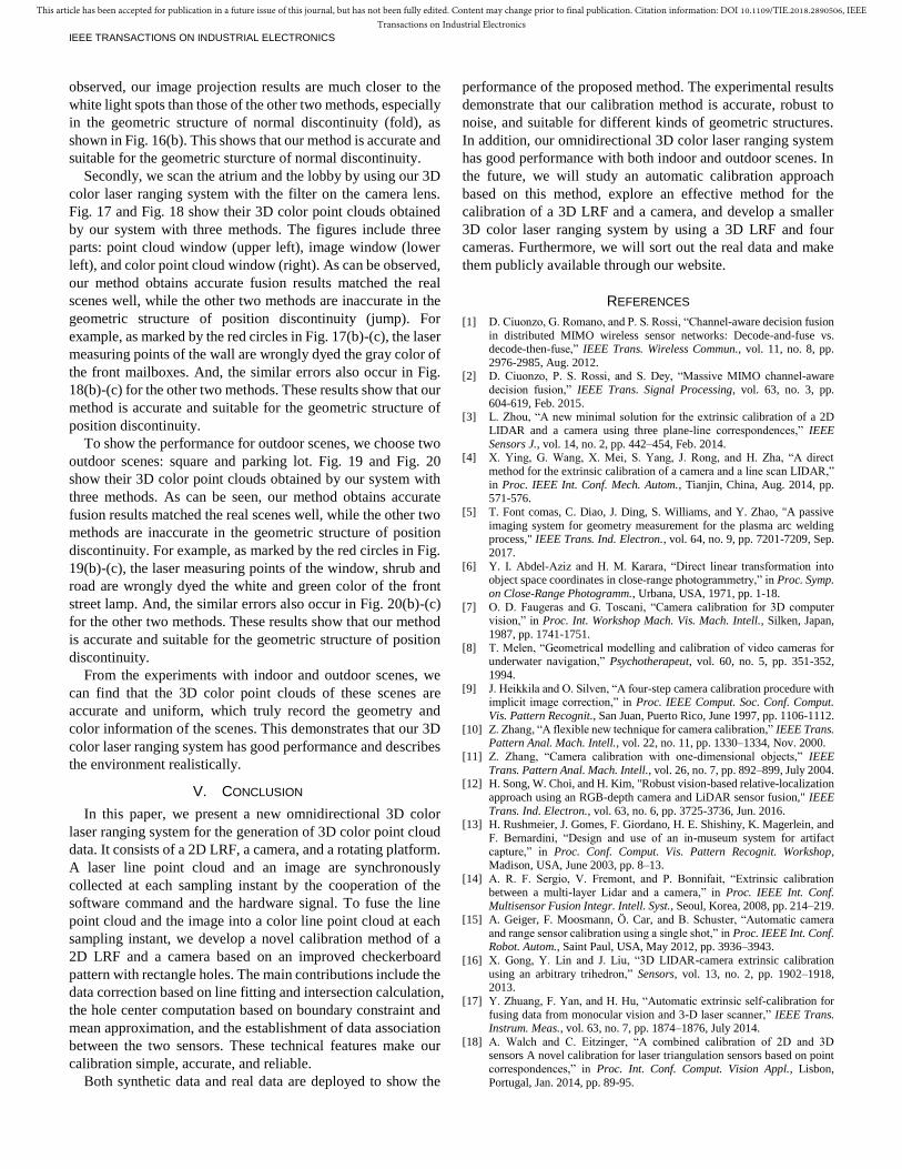
IEEE TRANSACTIONS ON INDUSTRIAL ELECTRONICS
observed, our image projection results are much closer to the
white light spots than those of the other two methods, especially
in the geometric structure of normal discontinuity (fold), as
shown in Fig. 16(b). This shows that our method is accurate and
suitable for the geometric sturcture of normal discontinuity.
Secondly, we scan the atrium and the lobby by using our 3D
color laser ranging system with the filter on the camera lens.
Fig. 17 and Fig. 18 show their 3D color point clouds obtained
by our system with three methods. The figures include three
parts: point cloud window (upper left), image window (lower
left), and color point cloud window (right). As can be observed,
our method obtains accurate fusion results matched the real
scenes well, while the other two methods are inaccurate in the
geometric structure of position discontinuity (jump). For
example, as marked by the red circles in Fig. 17(b)-(c), the laser
measuring points of the wall are wrongly dyed the gray color of
the front mailboxes. And, the similar errors also occur in Fig.
18(b)-(c) for the other two methods. These results show that our
method is accurate and suitable for the geometric structure of
position discontinuity.
To show the performance for outdoor scenes, we choose two
outdoor scenes: square and parking lot. Fig. 19 and Fig. 20
show their 3D color point clouds obtained by our system with
three methods. As can be seen, our method obtains accurate
fusion results matched the real scenes well, while the other two
methods are inaccurate in the geometric structure of position
discontinuity. For example, as marked by the red circles in Fig.
19(b)-(c), the laser measuring points of the window, shrub and
road are wrongly dyed the white and green color of the front
street lamp. And, the similar errors also occur in Fig. 20(b)-(c)
for the other two methods. These results show that our method
is accurate and suitable for the geometric structure of position
discontinuity.
From the experiments with indoor and outdoor scenes, we
can find that the 3D color point clouds of these scenes are
accurate and uniform, which truly record the geometry and
color information of the scenes. This demonstrates that our 3D
color laser ranging system has good performance and describes
the environment realistically.
V. CONCLUSION
In this paper, we present a new omnidirectional 3D color
laser ranging system for the generation of 3D color point cloud
data. It consists of a 2D LRF, a camera, and a rotating platform.
A laser line point cloud and an image are synchronously
collected at each sampling instant by the cooperation of the
software command and the hardware signal. To fuse the line
point cloud and the image into a color line point cloud at each
sampling instant, we develop a novel calibration method of a
2D LRF and a camera based on an improved checkerboard
pattern with rectangle holes. The main contributions include the
data correction based on line fitting and intersection calculation,
the hole center computation based on boundary constraint and
mean approximation, and the establishment of data association
between the two sensors. These technical features make our
calibration simple, accurate, and reliable.
Both synthetic data and real data are deployed to show the
performance of the proposed method. The experimental results
demonstrate that our calibration method is accurate, robust to
noise, and suitable for different kinds of geometric structures.
In addition, our omnidirectional 3D color laser ranging system
has good performance with both indoor and outdoor scenes. In
the future, we will study an automatic calibration approach
based on this method, explore an effective method for the
calibration of a 3D LRF and a camera, and develop a smaller
3D color laser ranging system by using a 3D LRF and four
cameras. Furthermore, we will sort out the real data and make
them publicly available through our website.
REFERENCES
[1] D. Ciuonzo, G. Romano, and P. S. Rossi, “Channel-aware decision fusion
in distributed MIMO wireless sensor networks: Decode-and-fuse vs. decode-then-fuse,” IEEE Trans. Wireless Commun., vol. 11, no. 8, pp.
2976-2985, Aug. 2012. [2] D. Ciuonzo, P. S. Rossi, and S. Dey, “Massive MIMO channel-aware
decision fusion,” IEEE Trans. Signal Processing, vol. 63, no. 3, pp.
604-619, Feb. 2015. [3] L. Zhou, “A new minimal solution for the extrinsic calibration of a 2D
LIDAR and a camera using three plane-line correspondences,” IEEE
Sensors J., vol. 14, no. 2, pp. 442–454, Feb. 2014. [4] X. Ying, G. Wang, X. Mei, S. Yang, J. Rong, and H. Zha, “A direct
method for the extrinsic calibration of a camera and a line scan LIDAR,”
in Proc. IEEE Int. Conf. Mech. Autom., Tianjin, China, Aug. 2014, pp. 571-576.
[5] T. Font comas, C. Diao, J. Ding, S. Williams, and Y. Zhao, "A passive
imaging system for geometry measurement for the plasma arc welding
process," IEEE Trans. Ind. Electron., vol. 64, no. 9, pp. 7201-7209, Sep.
2017.
[6] Y. I. Abdel-Aziz and H. M. Karara, “Direct linear transformation into object space coordinates in close-range photogrammetry,” in Proc. Symp.
on Close-Range Photogramm., Urbana, USA, 1971, pp. 1-18.
[7] O. D. Faugeras and G. Toscani, “Camera calibration for 3D computer vision,” in Proc. Int. Workshop Mach. Vis. Mach. Intell., Silken, Japan,
1987, pp. 1741-1751.
[8] T. Melen, “Geometrical modelling and calibration of video cameras for underwater navigation,” Psychotherapeut, vol. 60, no. 5, pp. 351-352,
1994.
[9] J. Heikkila and O. Silven, “A four-step camera calibration procedure with implicit image correction,” in Proc. IEEE Comput. Soc. Conf. Comput.
Vis. Pattern Recognit., San Juan, Puerto Rico, June 1997, pp. 1106-1112.
[10] Z. Zhang, “A flexible new technique for camera calibration,” IEEE Trans. Pattern Anal. Mach. Intell., vol. 22, no. 11, pp. 1330–1334, Nov. 2000.
[11] Z. Zhang, “Camera calibration with one-dimensional objects,” IEEE
Trans. Pattern Anal. Mach. Intell., vol. 26, no. 7, pp. 892–899, July 2004. [12] H. Song, W. Choi, and H. Kim, "Robust vision-based relative-localization
approach using an RGB-depth camera and LiDAR sensor fusion," IEEE
Trans. Ind. Electron., vol. 63, no. 6, pp. 3725-3736, Jun. 2016. [13] H. Rushmeier, J. Gomes, F. Giordano, H. E. Shishiny, K. Magerlein, and
F. Bernardini, “Design and use of an in-museum system for artifact
capture,” in Proc. Conf. Comput. Vis. Pattern Recognit. Workshop, Madison, USA, June 2003, pp. 8–13.
[14] A. R. F. Sergio, V. Fremont, and P. Bonnifait, “Extrinsic calibration
between a multi-layer Lidar and a camera,” in Proc. IEEE Int. Conf. Multisensor Fusion Integr. Intell. Syst., Seoul, Korea, 2008, pp. 214–219.
[15] A. Geiger, F. Moosmann, Ö. Car, and B. Schuster, “Automatic camera
and range sensor calibration using a single shot,” in Proc. IEEE Int. Conf. Robot. Autom., Saint Paul, USA, May 2012, pp. 3936–3943.
[16] X. Gong, Y. Lin and J. Liu, “3D LIDAR-camera extrinsic calibration
using an arbitrary trihedron,” Sensors, vol. 13, no. 2, pp. 1902–1918, 2013.
[17] Y. Zhuang, F. Yan, and H. Hu, “Automatic extrinsic self-calibration for
fusing data from monocular vision and 3-D laser scanner,” IEEE Trans. Instrum. Meas., vol. 63, no. 7, pp. 1874–1876, July 2014.
[18] A. Walch and C. Eitzinger, “A combined calibration of 2D and 3D sensors A novel calibration for laser triangulation sensors based on point
correspondences,” in Proc. Int. Conf. Comput. Vision Appl., Lisbon,
Portugal, Jan. 2014, pp. 89-95.
0278-0046 (c) 2018 IEEE. Personal use is permitted, but republication/redistribution requires IEEE permission. See http://www.ieee.org/publications_standards/publications/rights/index.html for more information.
This article has been accepted for publication in a future issue of this journal, but has not been fully edited. Content may change prior to final publication. Citation information: DOI 10.1109/TIE.2018.2890506, IEEETransactions on Industrial Electronics
IEEE TRANSACTIONS ON INDUSTRIAL ELECTRONICS
[19] Q. Zhang and R. Pless, “Extrinsic calibration of a camera and laser range
finder (improves camera calibration),” in Proc. IEEE/RSJ Int. Conf. Intell. Robots Syst., Sendai, Japan, Sep./Oct. 2004, pp. 2301–2306.
[20] F. Vasconcelos, J. P. Barreto, and U. Nunes, “A minimal solution for the
extrinsic calibration of a camera and a laser-rangefinder,” IEEE Trans. Pattern Anal. Mach. Intell., vol. 34, no. 11, pp. 2097-2107, Nov. 2012.
[21] R. Gomez-Ojeda, J. Briales, E. Fernandez-Moral, and J. Gonzalez-
Jimenez, “Extrinsic calibration of a 2D laser-rangefinder and a camera based on scene corners,” in Proc. IEEE Int. Conf. Robot. Autom., Seattle,
USA, May 2015, pp. 3611–3616.
[22] J. Briales, and J. Gonzalez-Jimenez, “A minimal solution for the calibration of a 2D laser-rangefinder and a camera based on scene
corners,” in Proc. IEEE/RSJ Int. Conf. Intell. Robots Syst., Hamburg, Germany, Sep./Oct. 2015, pp. 1891-1896.
[23] Z. Hu, Y. Li, N. Li, and B. Zhao, “Extrinsic calibration of 2-D laser
rangefinder and camera from single shot based on minimal solution,” IEEE Trans. Instrum. Meas., vol. 65, no. 4, pp. 915-929, Apr. 2016.
Yi An received the B.S. degree in automation and the M.S. and Ph.D. degrees in control theory and control engineering from Dalian University of Technology, Dalian, China, in 2001, 2004, and 2011, respectively. From 2007 to 2011, he was a Lecture with the School of Control Science and Engineering, Dalian University of Technology, Dalian, China, where he has been an Associate Professor since 2012. His research interests include point cloud data processing, sensing and perception,
information fusion, robot vision, and intelligent robot.
Bo Li received the B.S. degree in automation from Dalian University of Technology, Dalian, China, in 2018. He is currently working towards the M.S. degree with the School of Control Science and Engineering, Dalian University of Technology, Dalian. His research interests include point cloud data processing, object identification, and environmental perception.
Huosheng Hu (M’94–SM’01) received the M.Sc. degree in industrial automation from Central South University, Changsha, China, in 1982, and the Ph.D. degree in robotics from the University of Oxford, Oxford, U.K., in 1993. He is currently a Professor with the School of Computer Science and Electronic Engineering, University of Essex, Colchester, U.K., where he is leading the Robotics Research Group. He has authored over 420 papers. His current research interests include robotics, human–robot
interaction, embedded systems, mechatronics, and pervasive computing. Prof. Hu is a Founding Member of the IEEE Robotics and Automation Society Technical Committee on Networked Robots, a fellow of the Institution of Engineering and Technology, and a Senior Member of the Association for Computing Machinery. He currently serves as an Editor-in-Chief of the International Journal of Automation and Computing and the online Robotics journal, and an Executive Editor of the International Journal of Mechatronics and Automation.
Xiaoli Zhou received the B.S. degree in automation from Hefei University of Technology, Hefei, China, in 2015. She is currently working towards the M.S. degree with the School of Control Science and Engineering, Dalian University of Technology, Dalian. Her research interests include point cloud data processing, camera calibration, and scene understanding.