Bulletin of the Technical Committee onData Engineering December 2009 …sites.computer.org/debull/A09dec/A09DEC-CD.pdf · · 2010-03-22Bulletin of the Technical Committee onData

Bulletin of the Technical Committee on

DataEngineeringDecember 2009 Vol. 31 No. 4 IEEE Computer Society

LettersLetter from the Editor-in-Chief . . . . . . . . . . . . . . . . . . . . . . . . . . . . . . . . . . . . . . . . . . . . . . . . . . . . . . David Lomet 1Report: 4th Int’l Workshop on Self-Managing Database Systems (SMDB 2009) . . . . . . . . . . . . . . . . . . . . . . . . . . .

. . . . . . . . . . . . . . . . . . . . . . . . . . . . . . . . . . . . . . . . . . . . . . . . . . . . . . . . Ashraf Aboulnaga and Kenneth Salem 2Letter from the Special Issue Editors . . . . . . . . . . . . . . . . . . . . . . . . . . Marios Hadjieleftheriou, Vassilis J. Tsotras 6

Special Issue on Result Diversity

An Axiomatic Framework for Result Diversification . . . . . . . . . . . . . . . . . . Sreenivas Gollapudi, Aneesh Sharma 7The KNDN Problem: A Quest for Unity in Diversity . . . . . . . . . . . . . . . . . . . . . . . . . . . . . . . . . . Jayant R. Haritsa 15Making Product Recommendations More Diverse . . . . . . . . . . . . . . . . . . . . . . Cai-Nicolas Ziegler, Georg Lausen 23Battling Predictability and Overconcentration in Recommender Systems . . . . . . . . . . . . . . . . . . . . . . . . . . . . . . . . .

. . . . . . . . . . . . . . . . . . . . . . . . . . . . . Sihem Amer-Yahia, Laks V.S. Lakshmanan, Sergei Vassilvitskii, Cong Yu 33Addressing Diverse User Preferences: A Framework for Query Results Navigation . . . . . . Zhiyuan Chen, Tao Li 41Diversity over Continuous Data . . . . . . . . . . . . . . . . . . . . . . . . . . . . . . . . . . . . Marina Drosou, Evaggelia Pitoura 49Efficient Computation of Diverse Query Results . . . . . . Erik Vee, Jayavel Shanmugasundaram, Sihem Amer-Yahia 57Diversity in Skylines . . . . . . . . . . . . . . . . . . . . . . . . . . . . . . . . . . . . . . . . . . . . . . . . . . . . . . . . . . . . . . . . . . Yufei Tao 65

Conference and Journal NoticesICDE 2010 Conference . . . . . . . . . . . . . . . . . . . . . . . . . . . . . . . . . . . . . . . . . . . . . . . . . . . . . . . . . . . . . . . . . . . . . . . . 73VLDB 2010 Conference . . . . . . . . . . . . . . . . . . . . . . . . . . . . . . . . . . . . . . . . . . . . . . . . . . . . . . . . . . . . . . . . . . . . . . 74Symposium on Cloud Computing . . . . . . . . . . . . . . . . . . . . . . . . . . . . . . . . . . . . . . . . . . . . . . . . . . . . . . . . . .back cover

Editorial Board

Editor-in-ChiefDavid B. LometMicrosoft ResearchOne Microsoft WayRedmond, WA 98052, [email protected]

Associate EditorsSihem Amer-YahiaYahoo! Research111 40th St, 17th floorNew York, NY 10018

Beng Chin OoiDepartment of Computer ScienceNational University of SingaporeComputing 1, Law Link, Singapore 117590

Jianwen SuDepartment of Computer ScienceUniversity of California - Santa BarbaraSanta Barbara, CA 93106

Vassilis J. TsotrasDept. of Computer Science and Engr.University of California - RiversideRiverside, CA 92521

The TC on Data EngineeringMembership in the TC on Data Engineering is open

to all current members of the IEEE Computer Societywho are interested in database systems. The TC onData Engineering web page ishttp://tab.computer.org/tcde/index.html.

The Data Engineering BulletinThe Bulletin of the Technical Committee on Data

Engineering is published quarterly and is distributedto all TC members. Its scope includes the design,implementation, modelling, theory and application ofdatabase systems and their technology.

Letters, conference information, and news should besent to the Editor-in-Chief. Papers for each issue aresolicited by and should be sent to the Associate Editorresponsible for the issue.

Opinions expressed in contributions are those of theauthors and do not necessarily reflect the positions ofthe TC on Data Engineering, the IEEE Computer So-ciety, or the authors’ organizations.

The Data Engineering Bulletin web site is athttp://tab.computer.org/tcde/bull_about.html.

TC Executive Committee

ChairPaul LarsonMicrosoft ResearchOne Microsoft WayRedmond WA 98052, [email protected]

Vice-ChairCalton PuGeorgia Tech266 Ferst DriveAtlanta, GA 30332, USA

Secretary/TreasurerThomas RisseL3S Research CenterAppelstrasse 9aD-30167 Hannover, Germany

Past ChairErich NeuholdUniversity of ViennaLiebiggasse 4A 1080 Vienna, Austria

Chair, DEW: Self-Managing Database Sys.Anastassia AilamakiEcole Polytechnique Federale de LausanneCH-1015 Lausanne, Switzerland

Geographic CoordinatorsKarl Aberer (Europe)Ecole Polytechnique Federale de LausanneBatiment BC, Station 14CH-1015 Lausanne, Switzerland

Masaru Kitsuregawa (Asia)Institute of Industrial ScienceThe University of TokyoTokyo 106, Japan

SIGMOD LiasonYannis IoannidisDepartment of InformaticsUniversity Of Athens157 84 Ilissia, Athens, Greece

DistributionIEEE Computer Society1730 Massachusetts AvenueWashington, D.C. 20036-1992(202) [email protected]

i

Letter from the Editor-in-Chief

About the Bulletin

Work is progressing on converting issues from 1998 onward to a new web page format for accessing individualpapers. I would urge you to check out past issues in addition to the current issue to take note of the progress.While more remains to be done, all pages now have a standard, well formatted header. Going forward, thisshould also (eventually) reduce the work I need to do to generate an issue, as pages on both the ComputerSociety site and the Microsoft site are now identical.

Please do take a look at the web pages providing access to individual papers, and report any problems to me.Thank you.

I am considering dropping some versions of past issues from the web site. Before doing so, I wanted to giveyou advance notice so that you could provide input to this process. In particular, I plan to drop all the “draft”postscript versions from the web site. I may go on to drop “final” postscript versions as well. That would leaveonly the PDF version. Essentially everyone has access to a PDF reader, and PDF, being compressed, downloadsfaster. Again, please provide input to this process, especially if you would like to continue accessing postscriptversions.

The Current Issue

The “search” area continues to be of intense interest, both as a technical challenge and as a competitive arena.There is strong recognition that not everyone is interested in the same topic when a collection of key words areentered for search. There is much to be gained in making sure that other meanings are considered, and in manycases, that appropriate pages are also returned as results.

It is not only the case that diversity of result increases the likelihood of a web surfer finding the informationdesired. It is also true that search providers, when recognizing this diversity, increase the likelihood of placingadds of interest to the web surfer. This translates into more profit, and drives what seens to me to be the virtuouscycle of improved technology helping users and also rewarding commercial ventures that provide it.

In this fast moving field, today’s research leads quickly to tomorrow’s search offering. Vassilis Tsotrasand Marios Hadjieleftheriou have succeeded in bringing together research from both academic and industrialresearchers in this wide ranging snapshot of the current state of search and its diverse answers. As I have saidbefore, this is something that the Bulletin strives to do, providing a view of a field that is difficult to find in themore traditional venues. I want to thank both Vassilis and Marios for their hard work and success with this issue.I am sure you will find reading it to be valuable.

Self-managing Database Systems Workshop

I want to draw your attention to the report on the 4th workshop on “self managing database systems”. TheTechnical Committee on Data Engineering has one sub-committee, and it is on self-managing database system.This sub-group organizes an annual workshop held in conjunction with the ICDE conference. This is an activegroup, and reading the workshop report is a good way to stay up-to-date on this important area.

David LometMicrosoft Corporation

1

Report: 4th Int’l Workshop on Self-Managing Database Systems(SMDB 2009)

Ashraf Aboulnaga and Kenneth SalemUniversity of Waterloo

ashraf,[email protected]://db.uwaterloo.ca/tcde-smdb/smdb09

1 Introduction

The Fourth International Workshop on Self-Managing Database Systems took place on March 29th, 2009 inShanghai, China, on the day before ICDE. The SMDB workshops bring together researchers and practitionersinterested in making data management systems easier to deploy and operate effectively. Topics of interest rangefrom “traditional” management issues, such as database physical design, system tuning, and resource allocationto more recent challenges around scalable and highly-available data services in cloud computing environments.The SMDB Workshops are sponsored by the IEEE TCDE Workgroup on Self-Managing Database Systems.

The SMDB 2009 program began with a keynote presentation by James Hamilton, Vice President and Dis-tinguished Engineer with Amazon Web Services. This was followed by five technical papers, presented in twosessions. The workshop concluded with a panel discussion on “grand challenges” in database self-management.More information about the workshop program, including links to papers and presentation slides, can be foundat the SMDB 2009 web site, at http://db.uwaterloo.ca/tcde-smdb/smdb09.

2 Keynote

James Hamilton is a Vice President and Distinguished Engineer with Amazon Web Services. His back-ground includes 15 years in database engine development with IBM and Microsoft and 5 years inthe cloud service space with Microsoft and Amazon. He is also the author of widely-read blog, athttp://perspectives.mvdirona.com/. James’ keynote presentation was titled “Cloud-ComputingEconomies of Scale”. It covered hardware trends affecting cloud computing and a variety of useful techniquesfor scaling cloud services.

James began his presentation with a discussion of the economies of scale in networking, storage, and admin-istration that are achievable by very large scale cloud service providers like Amazon. He observed that whilethe largest cost component in enterprise data centers is typically people (administrators), this is not true for verylarge scale cloud service providers. For these organizations, costs are dominated by hardware, cooling, powerand power distribution. His figures showed power and power-related costs approaching 50% of total expensesand trending upwards, while hardware costs are trending down.

Copyright 2009 IEEE. Personal use of this material is permitted. However, permission to reprint/republish this material foradvertising or promotional purposes or for creating new collective works for resale or redistribution to servers or lists, or to reuse anycopyrighted component of this work in other works must be obtained from the IEEE.Bulletin of the IEEE Computer Society Technical Committee on Data Engineering

2

James next addressed the question of what ultimately limits the application of arbitrarily large amounts ofcomputing power to cloud applications. He argued that one limiting factor is power, since it is likely to becomethe dominant cost component for cloud providers. The other limiting factor is communications - the need toget data to the processors. In James’ words, the “CPUs are outpacing all means to feed them”. He noted thewidening “storage chasm” between DRAM and disks, which is encouraging larger memories and more disks.Finally, he noted the large and growing gap between sequential and random disk bandwidth.

In the last part of his presentation, James covered a variety of useful techniques for building scalable services.First, since scalable and highly-available services demand partitioning and redundancy, it is necessary to buildsuch services on top of large numbers of unreliable, distributed hardware and software components. Jamesargued that recovery-oriented computing [1] is the only affordable administrative model when there are manycomponents. This involves deeply monitoring applications and treating failures as routine occurrences to behandled, when possible, by simple automated recovery actions, such as rebooting and re-imaging. Humanadministrators become involved only if these automated steps do not work. Speaking of the limits of auto-administration, James noted that one should never allow an automated administration system to make a decisionthat would not be entrusted to a junior operations engineer.

Second, there are many techniques that can be used to lessen the impact of the disk/DRAM chasm, includingsequentialization of I/O workloads, the use of distributed memory caches, I/O cooling, and I/O concentration.On the subject of solid state storage devices (SSDs), James urged caution, noting that they should be used onlyif they produce a win in terms of work-per-dollar or work-per-joule. He argued that SSDs are “wonderful forsome workloads”, not plain wonderful.

Third, we should expect user data to be pulled closer to the edges of the network to support highly interactiveapplications and because of political and other restrictions on data movement. Conversely, we should expectaggregated data to be pulled towards the network core where it can be subjected to analysis. While growth intransactional workloads tends to be related to business growth, growth in analysis workloads is linked to the costof the analyses. As the cost of analysis drops, more types of analyses become economically viable.

Fourth, the spread between average and peak loads is high, so unmanaged load spikes will result in overload.Admission controls or service degradations are necessary to manage overload conditions. There are considerablepotential benefits around resource consumption shaping, e.g., “pushing” peak loads into load troughs.

James concluded by noting that utility computing is here to stay because of the cost advantages he hadalready described, and that the most difficult aspect of providing cloud computing services is “managing multi-center distributed partitioned redundant, data stores and caches”, which “really is a database problem.”

3 Paper Sessions

The five papers presented at the workshop dealt with a wide range of research issues related to self-managingdatabase systems. Belknap et al. [2] presented a fully automated workflow for tuning SQL queries that is partof Oracle Database 11g. The goal of this work is to automate the invocation of the SQL Tuning Advisor that isavailable in Oracle for tuning SQL statements, but that had to be invoked manually by the database administrator.The work identifies the SQL statements in the user workload that would be good candidates for automatic tuning.To ensure that recommended tuning actions do indeed result in improved performance, an interesting approachis adopted in which candidate query execution plans recommended by the tuner are executed and their actualperformance is measured to decide the best tuning action. Some safeguards are put in place to ensure that thetuner itself does not consume too much time and resources.

Thiem and Sattler [3] presented integrated performance monitoring in the Ingres database system. This isan approach for monitoring performance data at a high resolution from within the database system, with thegoal of providing a basis for better-informed automatic tuning decisions. The collected data includes CPU time,number of I/O’s, wall clock time, indexes used, and other performance metrics. A relational view over the in-

3

memory monitoring data is provided to users and tuning tools, and the data is also written to an on-disk workloaddatabase. The authors observe that collecting the monitoring data adds little overhead to the system, but writingit to the workload database is expensive, so a better mechanism for persisting the monitoring data is still needed.

Dash et al. [4] proposed an economic model for self-tuned caching in the cloud, specifically targeting sci-entific applications. The setting considered by the paper is one in which scientific data is stored in a cloud ofdatabases, and users pose queries against this data. The focus of the paper is developing an economic model fordeciding which index structures to create for the offered user queries. This model balances the utility of an indexstructure to user queries against the cost of creating this index structure and the amount that users are willing topay for different levels of service.

Schnaitter and Polyzotis [5] presented a benchmark for evaluating online index tuning algorithms. Manyalgorithms for online index selection have been proposed, so a principled approach for evaluating them is def-initely welcome. The proposed benchmark models a database hosting environment in which multiple data setsare hosted on one server and multiple workload suites are executed against these data sets. The workload suitesinclude SQL statements of varying complexity, and the benchmark shifts between these workload suites to modeldynamic workload behavior. The benchmark’s effectiveness was demonstrated by using it to compare two onlineindex selection algorithms implemented in PostgreSQL.

Finally, Hose et al. [6] presented an online approach for selecting materialized views in an OLAP environ-ment. The proposed approach targets OLAP server middleware that uses a data cube as the logical model andtranslates multi-dimensional queries into SQL queries over a relational star schema. These SQL queries are typ-ically expensive, and materialized views that pre-aggregate the data are often used to speed them up. The paperpresents an approach for choosing the set of materialized views for a workload and adjusting this set over time inan online manner. This requires a query representation that identifies how pre-computed aggregates can be usedto answer a query, a cost model to estimate the cost of a query if some set of aggregates is materialized, and asearch algorithm to identify the aggregates to pre-compute and materialize at each stage of workload execution.

4 Closing Panel

The workshop concluded with a panel on “Grand Challenges in Database Self-Management”, with six distin-guished panelists: Anastassia Ailamaki from Ecole Polytechnique Federale de Lausanne, Shivnath Babu fromDuke University, Nicolas Bruno from Microsoft Research, Benoit Dageville from Oracle, James Hamilton fromAmazon, and Calisto Zuzarte from the IBM Toronto Software Lab.

The panelists presented a wide range of views on the research challenges in the area of database self-management. Bruno presented the need for better modeling of query execution times (e.g., by modeling concur-rency and locking) and richer workload models (e.g., taking into account stored procedures with conditionals).He mentioned other challenges such as developing benchmarks for physical design tools (the problem addressedin [5]), extending self-management techniques to the cloud, exploiting large user bases to extract data and diag-nose problems, and developing a unifying theory for self-tuning database systems.

Dageville presented some of the work that Oracle has recently done on database manageability, coveringareas such as statistics collection, SQL tuning, memory management, and SQL repair. Looking ahead, he sawthe need for dealing with bad SQL statements from application developers with little database expertise, and forrobust query execution plans. He also saw the need for working towards proactively fixing problems before theyoccur, for example by leveraging the experience of other users. Another important area he identified is extendingmanageability solution to the entire software stack, beyond just the database system.

Ailamaki focused on using self-managing database systems in e-science. She mentioned that an importantchallenge in e-science is the sheer scale of the data. She pointed out that in this setting there are many aspects of adatabase systems that need to be self-managed, such as logical and physical design, power and energy awareness,and resource utilization. The responsibilities of the database management layer also include ensuring policy

4

compliance, allocating resources for scaling, and handling failures. She listed open problems including dynamicor underspecified workloads, non-relational data models, changes in database statistics, enabling scalability, andfinding a path for deploying research ideas to the scientists using e-science systems.

Hamilton pointed out that relational database systems are losing workloads in the cloud. Many cloud applica-tions use database systems, but most of the complexity (e.g., partitioning) is handled above the database system.Furthermore, many new applications use non-relational data models and many interesting workloads have leftrelational database systems. For example, analysis workloads are being handled by Hadoop, and caching is han-dled by memcached and similar solutions. Database infrastructures that focus on simplicity and scalability arebecoming increasingly popular. These include BigTable, Amazon SimpleDB, Facebook Cassandra, BerkelyDB,and many others. Hamilton identified several problems causing relational database systems to lose ground in thecloud: lack of scalability, excess administrative complexity, resource intensity due to un-needed features, unpre-dictable response times, excessively random data access patterns, opaque failure modes, and slow adaptabilityto new workloads. The solution he proposed involves supporting simple caching models and richer executionmodels, and embracing recovery-oriented computing to improve robustness.

Zuzarte observed that computing has gone from centralized mainframes to distributed client-server systems,and now back to a centralized system with dumb clients talking to a cloud. The challenges he posed includeoptimizing for objectives other than minimizing elapsed time or resource consumption; for example, minimizingenergy consumption or cloud computing dollar costs. He also observed that the Map-Reduce paradigm can ben-efit from techniques developed in the context of traditional database systems such as sharing scans, progressivere-optimization, and on-the-fly indexing.

Babu advocated using an experiment-driven approach for tuning and problem determination. This approachprovides simple and robust solutions to many manageability problems, but it poses several challenges suchas identifying the right type of experiment for a given problem and planning the sequence of experiments toconduct. Other challenges include providing an infrastructure for running experiments (e.g., in the cloud) andcombining experiment-driven management with current database tuning tools.

5 SMDB 2010

SMDB 2010 is being organized by Shivnath Babu and Kai-Uwe Sattler, and is scheduled for March 1, 2010 inLong Beach, California, immediately preceding ICDE 2010. Its scope includes emerging research areas arounddatabase self-management, such as cloud computing, multi-tenant databases, storage services, and datacenteradministration. Visit http://db.uwaterloo.ca/tcde-smdb/smdb10 for more information.

References[1] D. Patterson et al. Recovery oriented computing (ROC): Motivation, definition, techniques. Technical Report CSD-

02-1175, Berkeley, CA, USA, 2002.[2] Peter Belknap, Benoit Dageville, Karl Dias, and Khaled Yagoub. Self-tuning for SQL performance in Oracle Database 11g.

In Proc. SMDB’09, pages 1694–1700. IEEE Computer Society, 2009.[3] Alexander Thiem and Kai-Uwe Sattler. An integrated approach to performance monitoring for autonomous tuning. In

Proc. SMDB’09, pages 1671–1678. IEEE Computer Society, 2009.[4] Debabrata Dash, Verena Kantere, and Anastasia Ailamaki. An economic model for self-tuned cloud caching. In Proc.

SMDB’09, pages 1687–1693. IEEE Computer Society, 2009.[5] Karl Schnaitter and Neoklis Polyzotis. A benchmark for online index selection. In Proc. SMDB’09, pages 1701–1708.

IEEE Computer Society, 2009.[6] Katja Hose, Daniel Klan, and Kai-Uwe Sattler. Online tuning of aggregation tables for OLAP. In Proc. SMDB’09,

pages 1679–1686. IEEE Computer Society, 2009.

5

Letter from the Special Issue Editors

Users typically search the web by entering a small number of keywords in a search engine. The search engineuses an inverted index to identify all documents containing the keywords and ranks the results given some rel-evance function that depends on many different factors, including the query context, the application domain,location, temporal criteria, and more. Nevertheless, natural language is inherently ambiguous hence, to com-plicate matters further, expressing a query using a few keywords only, results in even larger inherent ambiguityand loss of relevant context. If a search engine does not consider the Diversity of query results during ranking,especially for queries with large ambiguity, the results produced will be unsatisfactory with high probability.A simple example is one of the most popular queries in YellowPages.com, Yahoo! Local and Google Maps:“Restaurant”. Depending on the query location, a typical search engine might rank a large number of Italian orChinese restaurants before the first Thai restaurant appears. Clearly, the user intent for this particular query isnot known, but it is safe to assume that since the user did not explicitly specify a particular cuisine, he/she mightbe interested in all options available in the vicinity of the query. It can be argued that diversification of resultswill invariably result in increased user satisfaction.

Query result diversity has been extensively studied the past few years and has gained traction in the indus-trial sector as well (for example, all major search engines implement some form of diversity ranking). Moreover,diversity is not limited to information retrieval. In general, it can be applied to any query that can return a verylarge number of results. Diversity based queries on traditional database systems, diversity in recommender sys-tems, diversity through user preferences, diversity in publish/subscribe systems, diversity on structured data,and diverse skyline computation using preference functions are some other application domains were diversifi-cation plays a big role in improving the end-user experience. This special issue of the Data Engineering Bulletinpresents a snapshot of the current state-of-art research on diversity for the aforementioned topics.

The first article [Gollapudi and Sharma] presents an axiomatic framework for diversification, formalizingthe problem and setting the stage for what follows. The second article [Haritsa] presents a diversity awarealgorithm for k-NN processing in traditional database systems. The third [Ziegler and Lausen] and fourth [Amer-Yahia, Lakshmanan, Vassilvitskii and Yu] articles discuss diversification in recommender systems, and morespecifically collaborative filtering. The article by [Chen and Li] focuses on efficient query evaluation based onpre-defined user preferences (as a means of expressing diversity). The article by [Drosou and Pitoura] discussescontent diversity in the case of continuous data delivery (in the context of publish/subscribe systems). The nextarticle [Vee, Shanmugasundaram, Amer-Yahia] talks about diversification of query results on structured data inthe presence of a preference hierarchy of attributes. The final article [Tao] discusses diversification of skylinequery results, based on user preference functions.

The goal of this special issue is to instigate further research into the essential problem of diversification.Even though these past few years there has been an impressive number of contributions of high quality into thisfield, we feel that there is still a lot of room for growth and improvement. It is our belief that current researchhas only scratched the surface of diversification in the respective domains, and the applications of diversificationwill keep growing. We would like to thank all authors for the time and effort they put into editing their excellentarticles for this special issue. We would also like to extend a special thanks to Marcos Vieira at UC Riversidefor editorial assistance with the issue.

Marios Hadjieleftheriou, Vassilis J. TsotrasAT&T Labs - Research UC Riverside

6

An Axiomatic Framework for Result Diversification∗

Sreenivas GollapudiMicrosoft Search Labs, Microsoft Research

[email protected]

Aneesh SharmaInstitute for Computational and Mathematical Engineering, Stanford University

[email protected]

Abstract

Informally speaking, diversification of search results refers to a trade-off between relevance and diversityin the set of results. In this article, we present a unifying framework for search result diversification usingthe axiomatic approach. The characterization provided by the axiomatic framework can help designand compare diversification systems, and we illustrate this using several examples. We also show thatseveral diversification objectives can be reduced to the combinatorial optimization problem of facilitydispersion. This reduction results in algorithms with provable guarantees for a number of well-knowndiversification objectives.

1 Introduction

In present day search engines, a user expresses her information need with as few query terms as possible. Insuch a scenario, a small number of terms often specify the intent in only an implicit manner. In the absence ofexplicit information representing user intent, the search engine needs to “guess” the results that are most likely tosatisfy different intents. In particular for an ambiguous query such as eclipse, the search engine could either takethe probability ranking principle approach of taking the “best guess” intent and showing the results, or it couldchoose to present search results that maximize the probability that a user with a random intent finds at least onerelevant document on the results page. This problem of the user not finding any any relevant document in herscanned set of documents is defined as query abandonment. Result diversification lends itself as an effectivesolution to minimizing query abandonment [1, 7, 16].

Intuitively, result diversification implies a trade-off between having more relevant results of the “most prob-able” intent and having diverse results in the top positions for a given query[4, 6]. The twin objectives of beingdiverse and being relevant often compete with each other, and any result diversification system must figure outhow to trade-off these two objectives appropriately. Therefore, result diversification can be viewed as combin-ing both ranking (presenting more relevant results in the higher positions) and clustering (grouping documentsatisfying similar intents) and therefore addresses a loosely defined goal of picking a set of most relevant but


∗An earlier version appeared in the Proceedings of the 18th International Conference on World Wide Web, 2009 [8].

7

novel documents. This resulted in the development of a set of very different objective functions and algorithmsranging from combinatorial optimizations [4, 16, 1] to those based on probabilistic language models [6, 20].The underlying principles supporting these techniques are often different and therefore admit different trade-offcriteria. Given the importance of the problem there has been relatively little work aimed at understanding resultdiversification independent of the objective functions or the algorithms used to solve the problem.

This article discusses an axiomatic framework for result diversification. We begin with a set of simple andnatural properties that any diversification system ought to satisfy and these properties help serve as a basisfor the space of objective functions for result diversification. We then analyze a few objective functions thatsatisfy different subsets of these properties. Generally, a diversification function can be thought of as takingtwo application specific inputs viz, a relevance function that specifies the relevance of document for a givenquery, and a distance function that captures the pairwise similarity between any pair of documents in the setof relevant results for a given query. In the context of web search, one can use the search engine’s rankingfunction1 as the relevance function. The characterization of the distance function is not that clear. In fact,designing the right distance function becomes a central factor to an effective result diversification. For example,by restricting the distance function to a metric by imposing the triangle inequality d(u,w) ≤ d(u, v) + d(v, w)for all u, v, w ∈ U , we can exploit efficient approximation algorithms to solve certain class of diversificationobjectives (see Section 3).

Our work is similar in spirit to earlier work on axiomatization of ranking and clustering systems [3, 11].We study the functions that arise out of the requirement of satisfying a set of simple properties and show animpossibility result which states that there exists no diversification function f that satisfies all the properties. Westate the properties in Section 2.

Although we do not aim to completely map the space of objective functions in this study, we show that somediversification objectives reduce to different versions of the well-studied facility dispersion problem. Specif-ically, we pick three functions that satisfy different subsets of the properties and characterize the solutionsobtained by well-known approximation algorithms for each of these functions. We also characterize some of theobjective functions defined in earlier works [1, 16, 6] using the axioms.

1.1 Related Work

The early work of [4] described the trade-off between relevance and novelty via the choice of a parameterizedobjective function. Subsequent work on query abandonment by [6] is based on the idea that documents should beselected sequentially according to the probability of the document being relevant conditioned on the documentsthat come before. [16] solved a similar problem by using bypass rates of a document to measure the overalllikelihood of a user bypassing all documents in a given set. Thus, the objective in their setting was to produce aset that minimized likelihood of completely getting bypassed.

[1] propose a diversification objective that tries to maximize the likelihood of finding a relevant documentin the top-k positions given the categorical information of the queries and documents. Other works on topicaldiversification include [18, 21]. [20, 19] propose a risk minimization framework for information retrieval thatallows a user to define an arbitrary loss function over the set of returned documents. [17] proposed a methodfor diversifying query results in online shopping applications wherein the query is presented in a structure formusing online forms.

Our work is based on axiomatizations of ranking and clustering systems [2, 11, 3]. [11] proposed a set ofthree natural axioms for clustering functions and showed that no clustering function satisfies all three axioms. [3]study ranking functions that combine individual votes of agents into a social ranking of the agents and comparethem to social choice welfare functions which were first proposed in the classical work on social choice theoryby [2].

1See [15] and references therein.

8

We also show a mapping from diversification functions to those used in facility dispersion [13, 12]. Theinterested reader will find a useful literature in the chapter on facility dispersion in [14, 5].

2 Axiomatic Framework

This section introduces the axiomatic framework and fixes the notation to be used in the remainder of thepaper. We are given a set U = u1, u2, . . . , un of n ≥ 2 of documents, and a finite set of queries Q. Now,given a query q ∈ Q and an integer k, we want to output a subset Sk ⊆ U (where |Sk| = k) of documentsthat is simultaneously both relevant and diverse.2 The relevance of each document is specified by a functionw : U × Q → R+, where a higher value implies that the document is more relevant to a particular query. Thediversification objective is intuitively thought of as giving preference to dissimilar documents. To formalizethis, we define a distance function d : U × U → R+ between the documents, where smaller the distance, themore similar the two documents are. We also require the distance function to be discriminative, i.e. for any twodocuments u, v ∈ U , we have d(u, v) = 0 if and only if u = v, and symmetric, i.e d(u, v) = d(v, u). Note thatthe distance function need not be a metric.

Formally, the set selection function f : 2U × Q × w × d → R can be thought of as assigning scores to allpossible subsets of U , given a query q ∈ Q, a weight function w(·), a distance function d(·, ·). Fixing q, w(·),d(·, ·) and a given integer k ∈ Z+ (k ≥ 2), the objective is to select a set Sk ⊆ U of documents such that thevalue of the function f is maximized, i.e. the objective is to find

S∗k = argmax

Sk⊆U, |Sk|=kf(Sk, q, w(·), d(·, ·)) (1)

where all arguments other than the set Sk are fixed inputs to the function.An important observation is that the diversification framework is under-specified and even if one assumes

that the relevance and distance functions are provided, there are many possible choices of the diversificationobjective function f . These functions could trade-off relevance and similarity in different ways, and one needsto specify criteria for selection among these functions. A natural mathematical approach in such a situation is toprovide axioms that any diversification system should be expected to satisfy and therefore provide some basis ofcomparison between different diversification functions.

2.1 Axioms of diversification

We propose that f is such that it satisfy the set of axioms given below, each of which is a property that is intuitivefor the purpose of diversification. In addition, we show that any proper subset of these axioms is maximal, i.e.no diversification function can satisfy all these axioms. This provides a natural method of selecting betweenvarious objective functions, as one can choose the essential properties for any particular diversification system.In section 3, we will illustrate the use of the axioms in choosing between different diversification objectives.Before we state the axioms, we state the following notation. Fix any q, w(·), d(·, ·), k and f , such that f ismaximized by S∗

k , i.e., S∗k = argmaxSk⊆U f(Sk, q, w(·), d(·, ·)).

1. Scale invariance: Informally, this property states that the set selection function should be insensitive tothe scaling of the input functions. Consider the optimal set S∗

k . Now, we require f to be such that we haveS∗k = argmaxSk⊆U f(Sk, q, α ·w(·), α · d(·, ·)) for any fixed positive constant α ∈ R, α > 0, i.e. S∗

k stillmaximizes f even if all relevance and distance values are scaled by some constant. Note that we require

2In this work, we focus our attention on the set selection problem instead of producing a ranked list as the output, which is theultimate goal in some settings such as web search. This choice is motivated by the fact that the set selection problem captures the coretrade-off involved in building a diversification system as we will see shortly. Furthermore, there are several ways to convert the selectedset into a ranked list. For instance, one can always rank the results in order of relevance.

9

the constant to be the same for both w(·) and d(·, ·) in order to be consistent with respect to the scale ofthe problem.

2. Consistency: Consistency states that making the output documents more relevant and more diverse, andmaking other documents less relevant and less diverse should not change the output of the ranking. Now,given any two functions α : U → R+ and β : U × U → R+, we modify the relevance and weightfunctions as follows:

w(u) =

w(u) + α(u) , u ∈ S∗

k

w(u)− α(u) , otherwise

d(u, v) =

d(u, v) + β(u, v) , u, v ∈ S∗

k

d(u, v)− β(u, v) , otherwise

The ranking function f must be such that it is still maximized by S∗k . We emphasize that the change in the

relevance and diversity for each document can be different, and consistency only requires the function fto be invariant with respect to the right direction of the change.

3. Richness: Informally speaking, the richness condition states that we should be able to achieve any possibleset as the output, given the right choice of relevance and distance function. This property is motivatedby the practical fact that one could construct a query (along with corresponding relevance and diversityfunctions) that would correspond to any given output set. Formally, there exists some w(·) and d(·, ·) suchthat for any k ≥ 2, there is a unique S∗

k which maximizes f .

4. Stability: The stability condition seeks to ensure that the output set does not change arbitrarily with theoutput size, i.e., the function f should be defined such that S∗

k ⊂ S∗k+1. One can also consider relaxations

of the strict stability condition such as |S∗k ∩ S∗

k+1| > 0. We do not discuss the relaxation further in thiswork.

5. Independence of Irrelevant Attributes: This axiom states that the score of a set is not affected by mostattributes of documents outside the set. Specifically, given a set S, we require the function f to be suchthat f(S) is independent of values of both w(u) and d(u, v) for all u, v /∈ S.

6. Monotonicity: Monotonicity simply states that the addition of any document does not decrease the scoreof the set. Fix any w(·), d(·, ·), f and S ⊆ U . Now, for any x /∈ S, we must have f(S ∪ x) ≥ f(S).

Finally, we state two properties that ensure that the diversification system will not trivially ignore one ofeither relevance or diversity objectives. This ensures that the system will capture the trade-off betweenthe two objectives in a non-degenerate manner.

7. Strength of Relevance: This property ensures that no function f ignores the relevance function. Formally,we fix some w(·), d(·, ·), f and S. Now, the following properties should hold for any x ∈ S:

(a) There exist some real numbers δ0 > 0 and a0 > 0, such that the condition stated below is satisfiedafter the following modification: obtain a new relevance function w′(·) from w(·), where w′(·) isidentical to w(·) except that w′(x) = a0 > w(x). The remaining relevance and distance valuescould decrease arbitrarily. Now, we must have

f(S,w′(·), d(·, ·), k) = f(S,w(·), d(·, ·), k) + δ0

10

(b) If f(S \x) < f(S), then there exist some real numbers δ1 > 0 and a1 > 0 such that the followingcondition holds: modify the relevance function w(·) to get a new relevance function w′(·) which isidentical to w(·) except that w′(x) = a1 < w(x). Now, we must have

f(S,w′(·), d(·, ·), k) = f(S,w(·), d(·, ·), k)− δ1

8. Strength of Similarity: This property ensures that no function f ignores the similarity function. Formally,we fix some w(·), d(·, ·), f and S. Now, the following properties should hold for any x ∈ S:

(a) There exist some real numbers δ0 > 0 and b0 > 0, such that the condition stated below is satisfiedafter the following modification: obtain a new distance function d′(·, ·) from d(·, ·), where we in-crease d(x, u) for the required u ∈ S to ensure that minu∈S d(x, u) = b0. The remaining relevanceand distance values could decrease arbitrarily. Now, we must have

f(S,w(·), d′(·, ·), k) = f(S,w(·), d(·, ·), k) + δ0

(b) If f(S \ x) < f(S), then there exist some real numbers δ1 > 0 and b1 > 0 such that thefollowing condition holds: modify the distance function d(·, ·) by decreasing d(x, u) to ensure thatmaxu∈S d(x, u) = b1. Call this modified distance function d′(·, ·). Now, we must have

f(S,w(·), d′(·, ·), k) = f(S,w(·), d(·, ·), k)− δ1

Given these axioms, a natural question is to characterize the set of functions f that satisfy these axioms. Asomewhat surprising observation here is that it is impossible to satisfy all of these axioms simultaneously (proofis in the full paper [8]):

Theorem 1: No function f satisfies all 8 axioms stated above.

This result allows us to naturally characterize the set of diversification functions, and selection of a particularfunction reduces to deciding upon the subset of axioms (or properties) that the function is desired to satisfy.The next section explore this idea further and shows that the axiomatic framework could be a powerful tool inchoosing between diversification function. Another advantage of the framework is that it allows a theoreticalcharacterization of the function which is independent of the specifics of the diversification system such as thedistance and the relevance function.

3 Objectives and Algorithms

In light of the impossibility result shown in Theorem 1, we can only hope for diversification functions that satisfya subset of the axioms. We note that the list of such functions is possibly quite large, and indeed several suchfunctions have been previously explored in the literature (see [6, 16, 1], for instance). Further, proposing a diver-sification objective may not be useful in itself unless one can actually find algorithms to optimize the objective.In this section, we aim to address both of the above issues: we demonstrate the power of the axiomatic frame-work in choosing objectives, and also propose reductions from a number of natural diversification objectives tothe well-studied combinatorial optimization problem of facility dispersion [14]. In particular, we propose twodiversification objectives in the following sections, and provide algorithms that optimize these objectives. Wealso present a brief characterization of the objective functions studied in earlier works [1, 16, 6]. We will use thesame notation as in the previous section and have the objective (namely equation 1), where f would vary fromone function to another. Also, we assume w(·), d(·, ·) and k to be fixed here and hence use the shorthand f(S)for the function.

11

3.1 Max-sum diversification

A natural bi-criteria objective is to maximize the sum of the relevance and dissimilarity of the selected set. Thisobjective can be encoded in terms of our formulation in terms of the function f(S), which is defined as follows:

f(S) = (k − 1)∑u∈S

w(u) + 2λ∑u,v∈S

d(u, v) (2)

where |S| = k, and λ > 0 is a parameter specifying the trade-off between relevance and similarity. Observe thatwe need to scale up the first sum to balance out the fact that there are k(k−1)

2 numbers in the similarity sum, asopposed to k numbers in the relevance sum. We first characterize the objective in terms of the axioms.

Remark 1: The objective function given in equation 2 satisfies all the axioms, except stability.

This objective can be recast in terms of a facility dispersion objective, known as the MAXSUMDISPERSION

problem. The MAXSUMDISPERSION problem is a facility dispersion problem having the objective maximizing thesum of all pairwise distances between points in the set S which we show to be equivalent to equation 2. To thisend, we define a new distance function d′(u, v) as follows:

d′(u, v) = w(u) + w(v) + 2λd(u, v) (3)

It is not hard to see the following claim (proof skipped):

Claim 2: d′(·, ·) is a metric if the distance d(·, ·) constitutes a metric.

Further, note that for some S ⊆ U (|S| = k), we have:∑u,v∈S

d′(u, v) = (k − 1)∑u∈S

w(u) + 2λ∑u,v∈S

d(u, v)

using the definition of d′(u, v) and the fact that each w(u) is counted exactly k − 1 times in the sum (as weconsider the complete graph on S). Hence, from equation 2 we have that

f(S) =∑u,v∈S

d′(u, v)

But this is also the objective of the MAXSUMDISPERSION problem described above where the distance metric isgiven by d′(·, ·).

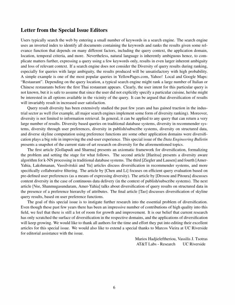
Given this reduction, we can map known results about MAXSUMDISPERSION to the diversification objective.First of all, we observe that maximizing the objective in equation 2 is NP-hard, but there are known approxima-tion algorithms for the problem. In particular, there is a 2-approximation algorithm for the MAXSUMDISPERSION

problem [10, 9] (for the metric case) and is given in algorithm 1. Hence, we can use algorithm 1 for the max-sumobjective stated in 2.

3.2 Mono-objective formulation

The space of diversification objectives is quite rich, and indeed there are several examples of objectives that donot reduce to facility dispersion. For instance, the second objective we will explore does not relate to facilitydispersion as it combines the relevance and the similarity values into a single value for each document (asopposed to each edge for the previous two objectives). The objective can be stated in the notation of ourframework in terms of the function f(S), which is defined as follows:

f(S) =∑u∈S

w′(u) (4)

12

Algorithm 1 Algorithm for MAXSUMDISPERSION

Require: Universe U , kEnsure: Set S (|S| = k) that maximizes f(S)

1: Initialize the set S = ∅2: for i← 1 to ⌊k2⌋ do3: Find (u, v) = argmaxx,y∈U d(x, y)4: Set S = S ∪ u, v5: Delete all edges from E that are incident to u or v6: end for7: if k is odd then8: add an arbitrary document to S9: end if

where the new relevance value w′(·) for each document u ∈ U is computed as follows:

w′(u) = w(u) +λ

|U | − 1

∑v∈U

d(u, v)

for some parameter λ > 0 specifying the trade-off between relevance and similarity. Intuitively, the value w′(u)computes the “global” importance (i.e. not with respect to any particular set S) of each document u. Theaxiomatic characterization of this objective is as follows:

Remark 2: The objective in equation 4 satisfies all the axioms except consistency.

Also observe that it is possible to exactly optimize objective 4 by computing the value w′(u) for all u ∈ Uand then picking the documents with the top k values of u for the set S of size k.

3.3 Other objective functions

We note that the link to the facility dispersion problem explored in section 3.1 is particularly rich as manydispersion objectives have been studied in the literature (see [14, 5]). Although we only explored a singleobjective here in order to illustrate the use of the dispersion objective, similar reductions can be used to obtainalgorithms with provable guarantees for many other diversification objectives [8].

The axiomatic framework can also be used to characterize diversification objectives that have been pro-posed previously. For instance, we note that the DIVERSIFYobjective function in [1] as well as the MINQUERY-ABANDONMENT formulations proposed in [16] violate the stability and the independence of irrelevant attributesaxioms.

4 Conclusions

This work presents an approach to characterizing diversification systems using a set of natural axioms. Thechoice of axioms presents an objective basis for characterizing diversification objectives independent of thealgorithms used, and the specific forms of the distance and relevance functions. Specifically, we illustrate theuse of the axiomatic framework by studying two objectives satisfying different subsets of axioms.

References[1] R. Agrawal, S. Gollapudi, A. Halverson, S. Ieong, Diversifying Search Results, in Proc. 2nd ACM Intl Conf on Web

Search and Data Mining, 5–14, 2009.

13

[2] K. Arrow, Social Choice and Individual Values, Wiley, New York, 1951.

[3] A. Altman, M. Tennenholtz, On the axiomatic foundations of ranking systems, in Proc. 19th Int’l Joint Conference onArtificial Intelligence, 917–922, 2005.

[4] J. Carbonell, J. Goldstein, The use of MMR, diversity-based reranking for reordering documents and producing sum-maries, in Proc. of the Int’l Conf. on Research and Development in Information Retrieval (SIGIR), 335–336, 1998.

[5] B. Chandra, M. M. Halldorsson, Approximation Algorithms for Dispersion Problems, in J. Algorithms, (38):2, 438–465, 2001.

[6] H. Chen, D. R. Karger, Less is more: probabilistic models for retrieving fewer relevant documents, in Proc. of the Int’lConf. on Research and Development in Information Retrieval (SIGIR), 429–436, 2006.

[7] C. L. A. Clarke, M. Kolla, G. V. Cormack, O. Vechtomova, A. Ashkan, S. Buttcher, I. MacKinnon, Novelty anddiversity in information retrieval evaluation, in Proc. of the Int’l Conf. on Research and Development in InformationRetrieval (SIGIR), 659–666, 2008.

[8] S. Gollapudi, A. Sharma, An Axiomatic Approach for Result Diversification, in Proc. of the Int’l Conf. on World WideWeb, 381–390, 2009.

[9] R. Hassin, S. Rubinstein, A. Tamir, Approximation algorithms for maximum dispersion, in Operations Research Let-ters, (21):3, 133–137, 1997.

[10] B. Korte, D. Hausmann, An Analysis of the Greedy Heuristic for Independence Systems, in Algorithmic Aspects ofCombinatorics, (2), 65–74, 1978.

[11] J. Kleinberg, An Impossibility Theorem for Clustering, in Advances in Neural Information Processing Systems 15:Proc. of the 2002 Conference, MIT Press, 2003.

[12] S. S. Ravi, D. J. Rosenkrantz, G. K. Tayi, Facility dispersion problems: Heuristics and special cases, in Proc. 2ndWorkshop on Algorithms and Data Structures (WADS), 355–366, 1991.

[13] S. S. Ravi, D. J. Rosenkrantz, G. K. Tayi, Heuristic and special case algorithms for dispersion problems, in Opera-tions Research, (42):2, 299–310, 1994.

[14] S. S. Ravi, D. J. Rosenkrantzt, G. K. Tayi, Approximation Algorithms for Facility Dispersion, in Handbook of Ap-proximation Algorithms and Metaheuristics, Chapman & Hall/CRC, 2007.

[15] S. Robertson, H. Zaragoza, On rank-based effectiveness measures and optimization, in Inf. Retr. (10):3, 321–339,2007.

[16] A. D. Sarma, S. Gollapudi, S. Ieong, Bypass rates: reducing query abandonment using negative inferences, in Proc.of the ACM SIGKDD Int’l Conf. on Knowledge Discovery and Data Mining, 177–185, 2008.

[17] E. Vee, U. Srivastava, J. Shanmugasundaram, P. Bhat, S. A. Yahia, Efficient Computation of Diverse Query Results,in IEEE 24th Int’l Conference on Data Engineering (ICDE), 228–236, 2008.

[18] C. X. Zhai, W. W. Cohen, J. Lafferty, Beyond independent relevance: methods and evaluation metrics for subtopicretrieval, in Proc. of the Int’l Conf. on Research and Development in Information Retrieval (SIGIR), 10–17, 2003.

[19] C. X. Zhai, Risk Minimization and Language Modeling in Information Retrieval, in Carnegie Mellon University,2002.

[20] C. X. Zhai and J. Lafferty, A risk minimization framework for information retrieval, in Information Processing andManagement, (42):1, 31–55, 2006.

[21] C. N. Ziegler, S. M. McNee, J. A. Konstan, G. Lausen, Improving recommendation lists through topic diversification,in Proc. of the Int’l Conf. on World Wide Web, 22–32, 2005.

14

The KNDN Problem: A Quest for Unity in Diversity

Jayant R. HaritsaIndian Institute of Science, Bangalore

[email protected]

Abstract

Given a query location Q in multi-dimensional space, the classical KNN problem is to return the Kspatially closest answers in the database with respect to Q. The KNDN (K-Nearest Diverse Neighbor)problem is a semantic extension where the objective is to return the spatially closest result set such thateach answer is sufficiently different, or diverse, from the rest of the answers. We review here the KNDNproblem formulation, the associated technical challenges, and candidate solution strategies.

1 Introduction

Over the last decade, the issue of diversity in query results produced by information retrieval systems, such assearch engines, has been investigated in great depth (see [11] for a recent survey). Curiously, however, there hasbeen relatively little diversity-related work with regard to queries issued on traditional database systems. Evenmore surprisingly, this paucity has occurred in spite of extensive research, during the same period, on supportingvanilla distance-based Top-K (or equivalently, KNN) queries in a host of database environments including onlinebusiness databases, multimedia databases, mobile databases, stream databases, etc. (see [2, 6, 7] for detailedsurveys). The expectation that this prior work would lead on to a vigorous investigation of result-set semantics,including aspects such as diversity, has unfortunately not fully materialized. In this article, we review our 2004study of database result diversity [9], in the hope that it may rekindle interest in the area. Specifically, wecover the KNDN (K-Nearest Diverse Neighbor) problem formulation, the associated technical challenges, andcandidate solution strategies.

Motivation. The general model of a KNN query is that there is a database of multidimensional objects againstwhich users submit point queries. Given a metric for measuring distances in the multidimensional space, thesystem is expected to find the K objects in the database that are spatially closest to the location of the user’squery. Typical distance metrics include the Euclidean and Manhattan norms. An example KNN applicationscenario is given below.

Example 1: Consider the situation where the London tourist office maintains the relation RESTAURANT(Name,Speciality,Rating,Expense), where Name is the name of the restaurant; Speciality indicates the foodtype (Greek, Chinese, Indian, etc.); Rating is an integer between 1 to 5 indicating restaurant quality; and, Ex-pense is the typical expected expense per person. In this scenario, a visitor to London may wish to submit


15

the KNN query shown in Figure 1(a) to have a choice of three nearby mid-range restaurants where dinner isavailable for around 50 Euros. (The query is written using the SQL-like notation described in [2].)

SELECT * FROM RESTAURANTWHERE Rating=3 and Expense=50ORDER 3 BY Euclidean

(a) KNN Query

G GreekC ChineseA American I Indian

Diverse

Nearest

30 90 110 50 70

4

5

3

2

1

0

Rat

ing

Expense

G G

G

G

I A

C

A C

G

Query

(Euro)

(b) Data Distribution

Figure 1: Motivational Example

For the sample distribution of data points in the RESTAURANT database shown in Figure 1(b), the aboveKNN query would return the answers shown by the circles. Note that these three answers are very similar:Parthenon-α,3,Greek,54, Parthenon-β,3,Greek,45, and Parthenon-γ,3,Greek,60. In fact, it is even pos-sible that the database may contain exact duplicates (wrt the Speciality, Rating and Expense attributes).

Returning three very similar answers may not offer much value to the London tourist. Instead, shemight be better served by being told, in addition to Parthenon-α,3,Greek,54, about a Chinese restaurantHunan,2,Chinese,40, and an Indian restaurant Taj,4,Indian,60, which would provide a close but more het-erogeneous set of choices to plan her dinner – these answers are shown by rectangles in Figure 1(b). In short, theuser would like to have not just the closest set of answers, but the closest diverse set of answers (an oft-repeatedquote from Montaigne, the sixteenth century French writer, is “The most universal quality is diversity” [15]).

2 The KNDN Problem

Based on the above motivation, we introduced five years ago the KNDN (K-Nearest Diverse Neighbor) problemin [9]. The objective here is to identify the spatially closest set of answers to the user’s query location such thateach answer is sufficiently diverse from all the others in the result set.

We began by modeling the database as composed of N tuples over a D-dimensional space with each tuplerepresenting a point in this space. The user specifies a point query Q over an M -sized subset of these attributesS(Q) : (s1, s2, . . . , sM ), referred to as “spatial attributes”; and lists a L-sized subset of attributes V (Q) : (v1, v2,. . . , vL), on which she would like to have result diversity – these attributes are referred to as “diversity attributes”.The space formed by the diversity attributes is referred to as diversity-space. Note that the choice of the diversityattributes is orthogonal to the choice of the spatial attributes. Finally, the user also specifies K, the number ofdesired answers, and the expected result is a set of K diverse tuples from the database. Referring back to theLondon tourist example, the associated settings in this framework are D = 4,M = 2, s1 = Rating, s2 =Expense, L = 1, v1 = Speciality,K = 3.

For ease of exposition, we will hereafter assume that the domains of all attributes are numeric and normalizedto the range [0, 1], and that all diversity dimensions are equivalent in the user’s perspective. The relaxation ofthese assumptions is discussed in [8].

16

2.1 Diversity Measure

The next, and perhaps most important, question we faced was how to define diversity and quantify it as a mea-sure. Here, there were a variety of options, such as hashing-based schemes [1], or taxonomy-based schemes [10],but all these seem primarily suited for the largely unstructured domain of IR applications. In the structureddatabase world, however, we felt that diversity should have a direct physical association with the data tuples forit to be meaningful to users. Accordingly, we chose our definition of diversity based on the classical Gower co-efficient [3]. Here, the difference between two points is defined as a weighted average of the respective attributevalue differences. Specifically, we first compute the (absolute) differences between the attribute values of thesetwo points in diversity-space, sequence these differences in decreasing order of their values, and then label themas (δ1, δ2, . . . , δL). Next, we calculate divdist, the diversity distance between points P1 and P2 with respect todiversity attributes V (Q) as

divdist(P1, P2, V (Q)) =L∑

j=1

(Wj × δj) (5)

where the Wj’s are weighting factors for the differences. Since all δj’s are in the range [0, 1] (recall that thevalues on all dimensions are normalized to [0, 1]), and by virtue of the Wj assignment policy discussed below,diversity distances are also bounded in the range [0, 1].

The assignment of the weights is based on the principle that larger weights should be assigned to the largerdifferences. That is, in Equation 5, we need to ensure that Wi ≥Wj if i < j. The rationale for this assignment isas follows: Consider the case where point P1 has values (0.2, 0.2, 0.3), point P2 has values (0.19, 0.19, 0.29) andpoint P3 has values (0.2, 0.2, 0.27). Consider the diversity of P1 with respect to P2 and P3. While the aggregatedifference is the same in both cases, yet intuitively we can see that the pair (P1, P2) is more homogeneous ascompared to the pair (P1, P3). This is because P1 and P3 differ considerably on the third attribute as comparedto the corresponding differences between P1 and P2. In a nutshell, a pair of points that have higher variance intheir attribute differences are taken to be more diverse than a pair with lower variance.

Now consider the case where P3 has values (0.2, 0.2, 0.28). Here, although the aggregate difference ishigher for the pair (P1, P2), yet again it is pair (P1, P3) that appears more diverse since its difference on the thirdattribute is larger than any of the individual differences in pair (P1, P2).

Based on the above observations, we decided that the weighting function should have the following proper-ties: First, all weights should be positive, since having differences in any dimension should never decrease thediversity. Second, the sum of the weights should add up to 1 (i.e.,

∑Lj=1Wj = 1) to ensure that divdist values

are normalized to the [0, 1] range. Third, the weights should be monotonically decaying (Wi ≥ Wj if i < j ) toreflect the preference given to larger differences. Finally, the weighting function should ideally be tunable usinga single parameter.

Example 2: A candidate weighting function that materially satisfies the above requirements is the following:

Wj =aj−1 × (1− a)

1− aL(1 ≤ j ≤ L) (6)

where a is a tunable parameter over the range (0, 1). Note that this function implements a geometric decay, withthe parameter ‘a’ determining the rate of decay. Values of a that are close to 0 result in faster decay, whereasvalues close to 1 result in slow decay. When the value of a is nearly 0, almost all weight is given to the maximumdifference i.e., W1 ≃ 1, modeling the L∞ (i.e., Max) distance metric, and when a is nearly 1, all attributes aregiven similar weights, modeling a L1 (i.e., Manhattan) distance metric.

Figure 2 shows, for different values of the parameter ‘a’ in Equation 6, the locus of points which have adiversity distance of 0.1 with respect to the origin (0, 0) in two-dimensional diversity-space.

17

Figure 2: Locus of Diversity=0.1 Points

SELECT * FROM RESTAURANTWHERE Rating=3 and Expense=50ORDER 3 BY EuclideanWITH MinDiv=0.1 ON Speciality

Figure 3: KNDN Query Example

2.1.1 Minimum Diversity Threshold

The next issue we faced was deciding the mechanism by which the user specified the extent to which diversitywas required in the result set. While complicated functions could be constructed for this purpose, we felt thattypical users of database systems would be only willing, or knowledgeable enough, to provide a single valuecharacterizing their requirements. Accordingly, we supported a single threshold parameter MinDiv, rangingbetween [0, 1]. Given this threshold setting, two points are diverse if the diversity distance between them isgreater than or equal to MinDiv. That is,

DIV (P1, P2, V (Q)) = true iff divdist(P1, P2, V (Q)) ≥MinDiv (7)

The advantage of the above simple definition is that it is amenable to a physical interpretation that canguide the user in determining the appropriate setting of MinDiv. Specifically, the interpretation is that if a pair ofpoints is deemed to be diverse, then these two points have a difference of MinDiv or more on atleast one diversitydimension. For example, a MinDiv of 0.1 means that any pair of diverse points differ in atleast one diversitydimension by atleast 10% of the associated domain size. In practice, we would expect that MinDiv settingswould be on the low side, typically not more than 0.2. Finally, note that the DIV function is commutative butnot transitive.

The notion of pair-wise diversity is easily extended to the final user requirement that each point in the resultset must be diverse with respect to all other points in the set. That is, given a result set A with answer pointsA1, A2, . . . , AK , we require DIV (Ai, Aj , V (Q)) = true ∀ i, j such that i = j and 1 ≤ i, j ≤ K. We callsuch a result set to be fully-diverse.

With the above framework, setting MinDiv to zero results in the traditional KNN query, whereas highervalues provide more and more importance to diversity at the expense of distance. The London tourist query cannow be stated as shown in Figure 3, where Speciality is the attribute on which diversity is calculated, and thegoal is to produce the spatially closest fully-diverse result set.

2.1.2 Integrating Diversity and Distance

Given a user query location and a diversity requirement, there may be multiple fully-diverse answer sets availablein the database. Ideally, the set that should be returned is the one that has the closest spatial characteristics. Toidentify this set, we need to first define a single value that characterizes the aggregate spatial distances of a set ofpoints, and this is done in the following manner: Let function SpatialDist(P,Q) calculate the spatial distanceof point P from query point Q. The choice of SpatialDist function is based on the user specification and could

18

be any monotonically increasing distance function such as Euclidean, Manhattan, etc. We combine distances ofall points in a set into a single value using an aggregate function Agg which captures the overall distance of theset from Q. While a variety of aggregate functions are possible, the choice is constrained by the fact that theaggregate function should ensure that as the individual points in the set move farther away from the query, thedistance of the set should also increase correspondingly. Sample aggregate functions which obey this constraintinclude the Arithmetic, Geometric, and Harmonic Means. Finally, we use the reciprocal of the aggregate todetermine the “closeness score” of the (fully-diverse) result set. Putting all these formulations together, given aquery Q and a candidate fully-diverse result set A with points A1, A2, . . . , AK , the closeness score of A withrespect to Q is computed as

CloseScore(A, Q) =1

Agg(SpatialDist(Q,A1), . . . , SpatialDist(Q,AK))(8)

2.1.3 Problem Formulation

The final KNDN problem formulation is as follows: Given a point query Q on a D-dimensional database, aMinDiv diversity threshold on a set of diversity dimensions V(Q), and a desired diverse-result cardinality of K,the goal of the K-Nearest Diverse Neighbor (KNDN) problem is to find the set of K mutually diverse tuples in thedatabase, whose CloseScore is the maximum, after including the spatially nearest tuple to Q in the result set.

The requirement that the nearest point to the user’s query should always form part of the result set is becausethis point, in a sense, best fits the user’s query. Further, the nearest point A1 serves to seed the result set sincethe diversity function is meaningful only for a pair of points. Since point A1 of the result is fixed, the result setsare differentiated based on their remaining (K − 1) choices.

3 Solution Techniques

Having described the KNDN problem formulation, we now move on to discussing the issues related to develop-ing solutions for this problem.

Not surprisingly, finding the optimal (wrt CloseScore) fully-diverse result set for the KNDN problem turnsout to be computationally hard. We can establish this by mapping KNDN to the well known independent setproblem [4] which is NP-complete. The mapping is achieved by forming a graph corresponding to the datasetin the following manner: Each tuple in the dataset forms a node in the graph and a edge is added between twonodes if the diversity between the associated tuples is less than MinDiv. Now any independent set of nodes,that is, a subgraph in which no two nodes are connected, of size K in this graph represents a fully-diverse setof K tuples. But finding any independent set, let alone the optimal independent set, is itself computationallyhard. Tractable solutions to the independent set problem have been proposed [4], but they require the graph to besparse and all nodes to have a bounded small degree. In our world, this translates to requiring that all the clustersin diversity-space should be small in size. But, this may not be typically true for the datasets encountered inpractice, rendering these solutions not generally applicable, and forcing us to go in for heuristic solutions instead.

3.1 Inadequacy of Clustering-based Solutions

At first glance, it may appear that a simple heuristic solution to the KNDN problem would be to initially groupthe data into clusters using algorithms such as BIRCH [13], replace all clusters by their representatives, and thenapply the traditional KNN approach on this summary database. There are two problems here: First, since theclusters are pre-determined, there is no way to dynamically specify the desired diversity, which may vary fromone user to another or may be based on the specific application that is invoking the KNDN search. Second, sincethe query attributes are not known in advance, we potentially need to identify clusters in all possible subspaces,

19

which may become infeasible due to the exponential number of such subspaces. Finally, this approach cannotprovide the traditional KNN results.

Yet another approach to produce a diverse result set could be to run the standard KNN algorithm, clusterits results, replace the clusters by their representatives, and then output these representatives as the diverse set.The problem with this approach is that it is not clear how to apriori determine the original number of requiredanswers such that there are finally K diverse representatives. If the original number is set too low, then thesearch process has to be restarted, whereas if the original number is set too high, a lot of wasted work ensues.

3.2 The MOTLEY Algorithm

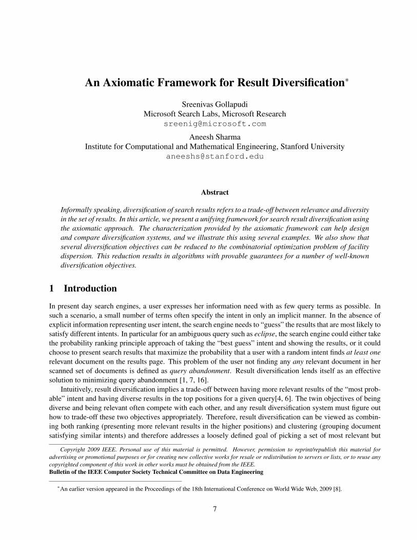
In light of the above, we designed a diversity-conscious greedy algorithm called MOTLEY1 for solving theKNDN problem, which is described in the remainder of this section.

3.2.1 Database Navigation

A major design issue in Motley was the mechanism chosen to navigate through the database. Two primaryapproaches for database navigation have been proposed in the extensive literaure on the vanilla KNN problem –the first is based on using standard database statistics (e.g., [2]), while the other is based on distance browsingusing spatial indices such as the R-tree (e.g., [6, 12]). We opted to use the latter approach since the detailedexperimental evaluation of [6] had indicated that distance browsing outperforms the alternative approaches –further, distance browsing can be seamlessly used for both KNN and KNDN problems.

In the distance browsing approach, the database tuples are processed incrementally in increasing order oftheir distance from the query location. The approach is predicated on having a containment-based index struc-ture, such as the R-tree[5], built collectively on all dimensions of the database (more precisely, the index needsto cover only those attributes on which spatial predicates may appear in the query workload). This assumptionappears practical since most current database systems natively support R-trees.

To implement distance browsing, a priority queue, pqueue, is maintained which is initialized with the rootnode of the R-Tree. The pqueue maintains the R-Tree nodes and data tuples in increasing order of their distancefrom the query location. While the distance between a data point and the query Q is computed in the standardmanner, the distance between a R-tree node and Q is computed as the minimum of the distances between Q andall points in the region enclosed by the MBR (Minimum Bounding Rectangle) of the R-tree node. The distanceof a node from Q is zero if Q is within the MBR of that node, otherwise it is the distance of the closest point onthe MBR periphery. For this, we first need to compute the distances between the MBR and Q along each querydimension – if Q is inside the MBR on a specific dimension, the distance is zero, whereas if Q is outside theMBR on this dimension, it is the distance from Q to either the low end or the high end of the MBR, whichever isnearer. Once the distances along all dimensions are available, they are combined (based on the distance metricin operation) to get the effective distance.

To return the next nearest neighbor, we pick up the first element of the pqueue. If it is a tuple, it is immedi-ately returned as the sought for neighbor. However, if the element is an R-tree node, all the children of that nodeare inserted in the pqueue. During this insertion process, the spatial distance of the object from the query pointis calculated and used as the insertion key. This process is repeated until we find a tuple to be the first elementof the queue, which is then returned.

The above distance browsing process continues until either the diverse result set is found, or until all pointsin the database are exhausted, signaled by the pqueue becoming empty.

1Motley: A collection containing a variety of sorts of things [14].

20

Q Pdivdist > 0.1

P

P

P

P5

3

4

21

divdist < 0.1

divdist < 0.1

Figure 4: Immediate Greedy

R2

P1

R1

P2

Rm

Rm

L

Tnew

Q

Figure 5: Buffered Greedy

3.2.2 Immediate Greedy

The first solution we attempted is called ImmediateGreedy (IG), wherein distance browsing is used to simplyaccess database tuples in increasing der of their spatial distances from the query point, as discussed above. Thefirst tuple is always inserted into the result set, A, to satisfy the requirement that the closest tuple to the querypoint must figure in the result set. Subsequently, each new tuple is added to A if it is diverse with respect to alltuples currently in A; otherwise, it is discarded. This process continues until A grows to contain K tuples.

While the IG approach is straightforward and easy to implement, there are cases where it may make poorchoices as shown in Figure 4. Here, Q is the query point, and P1 through P5 are the tuples in the database.Let us assume that the goal is to report 3 diverse tuples with MinDiv of 0.1. By inspection, we observe that theoverall best choice could be P1, P3, P4. But since DIV (P1, P2, V (Q)) = true, IG would include P2 andthis would then disqualify the candidatures of P3 and P4 as both DIV (P2, P3, V (Q)) and DIV (P2, P4, V (Q))are false. Eventually, Immediate Greedy would give the solution as P1, P2, P5. Worse, if point P5 happensto be not present in the database, then this approach will fail to return a fully-diverse set even though such a set,namely P1, P3, P4, is available.

3.2.3 Buffered Greedy

The above problems are addressed in the BufferedGreedy (BG) method by recognizing that IG gets into difficultybecause, at all times, only the diverse points (or “leaders”) in the result set, retained. To counter this, BGmaintains with each leader a bounded buffered set of “dedicated followers” – a dedicated follower is a point thatis not diverse with respect to a specific leader but is diverse with respect to all remaining leaders.

Given this additional set of dedicated followers, we adopt the heuristic that a current leader, Li, is replacedin the result set by its dedicated followers F 1

i , F2i , . . . , F

ji (j > 1) as leaders if (a) these dedicated followers

are all mutually diverse, and (b) incorporation of these followers as leaders does not result in the prematuredisqualification of future leaders. The first condition is necessary to ensure that the result set contains onlydiverse points, while the second is necessary to ensure that we do not produce solutions that are worse thanImmediate Greedy. For example, if in Figure 4, point P5 had happened to be only a little farther than point P4

such that DIV (P2, P5, V (Q)) = true, then the replacement of P2 by P3 and P4 could be the wrong choicesince P1, P2, P5 may turn out to be the best solution.

To implement the second condition, we must know when it is “safe” to go ahead with a replacement i.e.,when it is certain that all future leaders will be diverse from the current set of followers. To achieve this, we dothe following: For each point, we consider a hypothetical sphere that contains all points in the domain space thatmay be non-diverse with respect to it. That is, we set the radius Rm of the sphere equal to the distance of thefarthest non-diverse point in the domain space. Note that this sphere may contain some diverse points as well,but our aim is to take a conservative approach. Now, the replacement of a leader by selected dedicated followerscan be done as soon as we have reached a distance greater than Rm with respect to the farthest follower from the

21

query – this is because all future leaders will be diverse with respect to selected dedicated followers and there isno possibility of disqualification beyond this point. To clarify this technique, consider the following example:

Example 3: In Figure 5, the circles around P1 and P2 show the areas that contain all points that are not diversewith respect to P1 and P2, respectively. During the distance browsing process, when we access the point Tnew

(Figure 5), we know that all future points will be diverse from P1 and P2. At this time, if P1 and P2 are dedicatedfollowers of L and mutually diverse, then we can replace L by P1, P2.

Our experimental results (detailed in [9, 8]) on synthetic and real data-sets, indicate that BufferedGreedy canprovide high-quality diverse solutions at a low cost in terms of both result distance and processing time.

4 Future Directions

In this article, we reviewed the KNDN problem of finding the closest set of answers such that the user willfind each answer sufficiently different from the rest, thereby adding value to the result set. This topic has beenlargely ignored by the database community, but appears to be a fecund source of interesting and challengingproblems. For example, handling diversity in high-dimensional data, and efficient maintenance and usage ofspatial index structures for arbitrary subsets of attributes, are promising immediate probems to be addressed. Inthe long term, modeling the KNDN operations within the query optimizer and integrating the solution with thequery processing engine would be of practical import.

References[1] A. Broder, M. Charikar, A. Frieze and M. Mitzenmacher, Min-wise independent permutations, Journal of Computer

and System Sciences, 60(3), 2000.[2] N. Bruno, S. Chaudhuri and L. Gravano, Top-K Selection Queries over Relational Databases: Mapping Strategies

and Performance Evaluation, ACM Trans. on Database Systems, 27(2), 2002.[3] J. Gower, A general coefficient of similarity and some of its properties, Biometrics 27, 1971.[4] M. Grohe, Parameterized Complexity for Database Theorists, SIGMOD Record 31(4), December 2002.[5] A. Guttman, R-trees: A dynamic index structure for spatial searching, Proc. of ACM SIGMOD Intl. Conf. on Man-

agement of Data, 1984.[6] G. Hjaltason and H. Samet, Distance Browsing in Spatial Databases, ACM Trans. on Database Systems, 24(2), 1999.[7] I. Ilyas, G. Beskales and M. Soliman, A Survey of Top-k Query Processing Techniques in Relational Database Sys-

tems, ACM Computing Surveys, 40(4), October 2008.[8] A. Jain, P. Sarda and J. Haritsa, Providing Diversity in K-Nearest Neighbor Query Results, Tech. Report TR-2003-04,

DSL/SERC, Indian Institute of Science, 2003.[9] A. Jain, P. Sarda, and J. Haritsa, Providing Diversity in K-Nearest Neighbor Query Results, Proc. of 8th Pacific Asia

Conf. on Knowledge Discovery and Data Mining, 2004.[10] S. Gollapudi and A. Sharma, An Axiomatic Approach for Result Diversification, Proc. of World Wide Web Conf.,

2009.[11] E. Minack, G. Demartini and W. Nejdl, Current Approaches to Search Result Diversification, Proc. of 1st Intl. Work-

shop on Living Web, 2009.[12] N. Roussopoulos, S. Kelley and F.Vincent, Nearest Neighbor Queries, Proc. of ACM SIGMOD Intl. Conf. on Man-

agement of Data, 1995.[13] T. Zhang, R. Ramakrishnan and M. Livny, BIRCH: An Efficient Data Clustering Method for Very Large Databases,

Proc. of ACM SIGMOD Intl. Conf. on Management of Data, 1996.[14] www.thefreedictionarity.com

[15] www.elibronquotations.com

22

Making Product Recommendations More Diverse

Cai-Nicolas Ziegler∗ Georg Lausen

Institut fur Informatik, Universitat FreiburgGeorges-Kohler-Allee, Gebaude 51

79110 Freiburg i. Br., Germany

cziegler,[email protected]

Abstract

Past research in recommender systems has mainly focused on improving accuracy, i.e., making eachsingle recommendation get as close to the user’s information need as possible. However, while this ap-proach works well when focusing on single recommendations as atomic entities, its usefulness to theconsumer appears limited when considering entire recommendation lists along with their overall util-ity, which often appear to provide rather an unbalanced diet to the user: Recommendation lists seldomreflect the consumer’s entire spectrum of interest but rather hook on to small portions that appear partic-ularly favorable with regard to accuracy optimization. We analyze the diversification issue in detail andpresent a framework that is geared towards making lists as interesting and colorful as possible, tradinga minimum of accuracy in exchange for the gain in diversity. Empirical evaluations aiming for actualuser satisfaction underpin the cogency of our approach.

1 Introduction

Recommender systems [10] intend to provide people with recommendations of products they will appreciate,based on their past preferences. Many of the most successful systems make use of collaborative filtering [6],and numerous commercial systems, e.g., Amazon.com’s recommender [9], exploit these techniques to offerpersonalized recommendation lists to their customers. Though the accuracy of state-of-the-art collaborativefiltering systems, i.e., the probability that the active user1 will appreciate the products recommended, is ex-cellent, some implications affecting user satisfaction have been observed in practice. Thus, on Amazon.com(http://www.amazon.com), many recommendations seem to be “similar” with respect to content. For instance,customers that have purchased many of Hermann Hesse’s prose may happen to obtain recommendation listswhere all top-5 entries contain books by that respective author only. When considering pure accuracy, all theserecommendations appear excellent since the active user clearly appreciates books written by Hermann Hesse.


∗Now working at The Boston Consulting Group, Munich. Contact at [email protected] term “active user” refers to the person for whom recommendations are made.

23

On the other hand, assuming that the active user has several interests other than Hermann Hesse, e.g., historicalnovels, the recommended set of items appears poor, owing to its lack of diversity.

Traditionally, recommender system projects have focused on optimizing accuracy. Now research has reachedthe point where going beyond pure accuracy and toward real user experience becomes indispensable for furtheradvances. This work looks specifically at impacts of recommendation lists, regarding them as entities in theirown right rather than mere aggregations of single and independent suggestions.

2 On Collaborative Filtering

Collaborative filtering (CF) still represents the most commonly adopted technique in recommender systems. Itsbasic idea is to make recommendations based upon ratings that users have assigned to products. Ratings caneither be explicit, i.e., by having the user state his opinion about a given product, or implicit, when the mere actof purchasing an item counts as an expression of appreciation. While implicit ratings are more facile to collect,their usage implies adding noise to the collected information.

User-based Collaborative Filtering has been explored in-depth during the last 10-15 years and is the mostpopular recommendation algorithm [6], owing to its compelling simplicity and excellent quality of recommen-dations. CF operates on a set of users A = a1, a2, . . . , an, a set of products B = b1, b2, . . . , bm, and partialrating functions ri : B → [−1,+1]⊥ for each user ai. Negative values ri(bk) denote utter dislike, while positivevalues express ai’s liking of product bk. If ratings are implicit only, we represent them by set Ri ⊆ B, equivalentto bk ∈ B | ri(bk) = ⊥. The user-based CF’s working process can be broken down as follows:

• Neighborhood formation. Assuming ai as the active user, similarity values c(ai, aj) ∈ [−1,+1] forall aj ∈ A \ ai are computed, based upon the similarity of their respective rating functions ri, rj . Ingeneral, Pearson correlation [12, 4] or cosine distance [6] are used for computing c(ai, aj). The top-Mmost similar users aj become members of ai’s neighborhood, clique(ai) ⊆ A.

• Rating prediction. Taking all the products bk that ai’s neighbors aj ∈ clique(ai) have rated and whichare new to ai, i.e., ri(bk) = ⊥, a prediction of liking wi(bk) is produced. Value wi(bk) hereby depends onboth the similarity c(ai, aj) of aj with rj(bk) = ⊥, as well as the ratings rj(bk) these aj assigned to bk.

Eventually, a list Pwi : 1, 2, . . . , N → B of top-N recommendations is computed, based on predictionswi. Pwi is injective and reflects recommendation ranking in descending order, giving highest predictions first.

Item-based CF has favorable computational complexity characteristics and allows to decouple the model com-putation process from actual prediction making. Specifically for cases where |A| ≫ |B|, item-based CF’scomputational performance has been shown superior to user-based CF [11]. Its success also extends to manycommercial recommender systems, such as Amazon.com’s [9].

As with user-based CF, recommendation making is based upon ratings ri(bk) that users ai ∈ A providedfor products bk ∈ B. However, unlike user-based CF, similarity values c are computed for items rather thanusers, hence c : B × B → [−1,+1]. Roughly speaking, two items bk, be are similar, i.e., have large c(bk, be),if users who rate one of them tend to rate the other, and if users tend to assign them identical or similar ratings.Moreover, for each bk, its neighborhood clique(bk) ⊆ B of top-M most similar items is defined.

3 Evaluation Metrics

Evaluation metrics are essential in order to judge the performance of recommender systems, even though theyare still in their infancies. Most evaluations concentrate on accuracy measurements only and neglect other fac-

24

tors, e.g., novelty and serendipity of recommendations, and the diversity of the recommended list’s items. Thefollowing sections give a short overview of popular metrics. An extensive survey of accuracy metrics is in [7].

3.1 Accuracy Metrics

Accuracy metrics have been proposed for two major tasks: First, to judge the accuracy of single predictions,i.e., how much predictions wi(bk) for products bk deviate from ai’s actual ratings ri(bk). These metrics areparticularly suited for tasks where predictions are displayed along with the product, e.g., annotation in context[7]. Examples include the mean absolute error (MAE), and mean squared error (MSE).

Second, decision-support metrics evaluate the effectiveness of helping users to select high-quality itemsfrom the set of all products, generally supposing binary preferences. Typical decision-support metrics includethe well-known precision and recall metrics, known from information retrieval, as well as ROC, the “receiveroperating characteristic” (see, e.g., [5]).

3.2 Beyond Accuracy

Though accuracy metrics are an important facet of usefulness, there are traits of user satisfaction they are unableto capture. However, non-accuracy metrics have largely been denied major research interest so far. Among allnon-accuracy evaluation metrics, coverage has been the most frequently used [6, 5]. Coverage measures thepercentage of elements part of the problem domain for which predictions can be made.

Some recommenders produce highly accurate results that are still useless in practice, e.g., suggesting bananasto customers in grocery stores. Though being highly accurate, note that almost everybody likes and buys bananas.Hence, their recommending appears far too obvious and of little help to the shopper. Novelty and serendipitymetrics thus measure the “non-obviousness” of recommendations made, avoiding “cherry-picking” [7]. For somesimple measure of serendipity, take the average popularity of recommended items.

3.3 Intra-List Similarity

We present a new metric that intends to capture the diversity of a list. Hereby, diversity may refer to all kinds offeatures, e.g., genre, author. Based upon an arbitrary function c : B × B → [−1,+1] measuring the similarityc(bk, be) between products bk, be according to some custom-defined criterion, we define intra-list similarity forai’s list Pwi as follows:

ILS(Pwi) =

∑bk ∈ℑPwi

∑be ∈ℑPwi , bk =be

c(bk, be)

2(9)

Symbol ℑPwi denotes the image of map Pwi , i.e., all items part of the recommendation list. Higher scoresof ILS(Pwi) denote lower diversity. An interesting mathematical feature of ILS(Pwi) we are referring to inlater sections is permutation-insensitivity, i.e., let SN be the symmetric group of all permutations on N = |Pwi |symbols, then ∀σi, σj ∈ SN : ILS(Pwi σi) = ILS(Pwi σj) holds. Hence, simply rearranging positions ofrecommendations in a top-N list Pwi does not affect Pwi’s intra-list similarity.

4 Topic Diversification

One major issue with accuracy metrics is their inability to capture the broader aspects of satisfaction, hidingblatant flaws in existing systems. For instance, suggesting a list of very similar items, e.g., with respect to theauthor, genre, or topic, may be of little use for the user, even though this list’s average accuracy might be high.The issue has been perceived by other researchers before, coined “portfolio effect” by Ali and van Stam [1]. Webelieve that item-based CF systems in particular are susceptible to that effect.

25

procedure diversify (Pwi , ΘF ) Bi ← ℑPwi ; Pwi∗(1)← Pwi(1);

for z ← 2 to N doset B′

i ← Bi \ Pwi∗(k) | k ∈ [1, z[ ;∀b ∈ B′: compute c∗(b, Pwi∗(k) | k ∈ [1, z[ );compute Pc∗ : 1, 2, . . . , |B′

i| → B′i using c∗;

for all b ∈ B′i do

P rev−1

c∗ (b)← |B′i| − P−1

c∗ (b);w∗i (b)← P−1

wi(b) · (1−ΘF ) + P rev−1

c∗ (b) ·ΘF ;

end doPwi∗(z)← minw∗

i (b) | b ∈ B′i;

end doreturn Pwi∗;

Algorithm 1: Sequential topic diversification

We propose an approach we call topic diversification to deal with the problem at hand and make recom-mended lists more diverse and thus more useful. Our method represents an extension to existing recommenderalgorithms and is applied on top of recommendation lists.

4.1 Taxonomy-based Similarity Metric

Function c∗ : 2B × 2B → [−1,+1], quantifying the similarity between two product sets, forms an essentialpart of topic diversification. We instantiate c∗ with our metric for taxonomy-driven filtering [13], though othercontent-based similarity measures may appear likewise suitable. Our metric computes the similarity betweenproduct sets based upon their classification. Each product belongs to one or more classes that are hierarchicallyarranged in classification taxonomies, describing the products in machine-readable ways.

Classification taxonomies exist for various domains. Amazon.com crafts very large taxonomies for books,DVDs, CDs, electronic goods, and apparel. Moreover, all products on Amazon.com bear content descriptionsrelating to these domain taxonomies. Featured topics could include author, genre, and audience.

4.2 Topic Diversification Algorithm

Algorithm 1 shows the complete topic diversification algorithm, a brief textual sketch is given in the next para-graphs.

Function Pwi∗ denotes the new recommendation list, resulting from applying topic diversification. For everylist entry z ∈ [2, N ], we collect those b from the candidate products set Bi that do not occur in positions o < zin Pwi∗ and compute their similarity with Pwi∗(k) | k ∈ [1, z[ containing all new recommendations precedingrank z.

Sorting all products b according to c∗(b) in reverse order, we obtain the dissimilarity rank P revc∗ . This rank

is then merged with the original recommendation rank Pwi according to diversification factor ΘF , yieldingfinal rank Pwi∗. Factor ΘF defines the impact that dissimilarity rank P rev

c∗ exerts on the eventual overall output.

26

Large ΘF ∈ [0.5, 1] favors diversification over ai’s original relevance order, while low ΘF ∈ [0, 0.5[ producesrecommendation lists closer to the original rank Pwi . For experimental analysis, we used factors ΘF ∈ [0, 0.9].

Note that ordered input lists Pwi must be considerably larger than the final top-N list. For our later experi-ments, we used top-50 input lists for eventual top-10 recommendations.

The effect of dissimilarity bears traits similar to that of osmotic pressure and selective permeability knownfrom molecular biology; this concept allows cells (i.e, recommendation lists) to maintain their internal compo-sition of substances (i.e., topics) at required levels (i.e., gauging accuracy versus dissimilarity) [14].

5 Empirical Analysis

We conducted offline evaluations to understand the ramifications of topic diversification on accuracy metrics, andonline analysis to investigate how our method affects actual user satisfaction. We applied topic diversificationwith ΘF ∈ 0, 0.1, 0.2, . . . 0.9 to lists generated by both user-based CF and item-based CF, observing effectsthat occur when steadily increasing ΘF and analyzing how both approaches respond to diversification.

We based online and offline analyses on data gathered from BookCrossing (http://www.bookcrossing.com).The latter community caters for book lovers exchanging books all around the world and sharing their expe-riences with others. We collected data on 278, 858 members of BookCrossing and 1, 157, 112 ratings, bothimplicit and explicit, referring to 271, 379 distinct ISBNs. Invalid ISBNs were excluded from the outset. Thecomplete BookCrossing dataset, featuring fully anonymized information, is available via the first author’s home-page (http://www.informatik.uni-freiburg.de/∼cziegler).

Next, we mined Amazon.com’s book taxonomy, comprising 13,525 distinct topics. In order to be able toapply topic diversification, we mined content information, focusing on taxonomic descriptions that relate booksto taxonomy nodes from Amazon.com. Since many books on BookCrossing refer to rare, non-English books, oroutdated titles not in print anymore, we were able to garner background knowledge for only 175, 721 books. Intotal, 466, 573 topic descriptors were found, giving an average of 2.66 topics per book.

Owing to the BookCrossing dataset’s extreme sparsity, we decided to further condense the set in order toobtain more meaningful results from CF algorithms when computing recommendations. Hence, we discardedall books missing taxonomic descriptions, along with all ratings referring to them. Next, we also removed booktitles with fewer than 20 overall mentions. Only community members with at least 5 ratings each were kept.

The resulting dataset’s dimensions were considerably more moderate, featuring 10, 339 users, 6, 708 books,and 361, 349 book ratings.

5.1 Offline Experiments

We performed offline experiments comparing precision, recall, and intra-list similarity scores for 20 different listsetups. Half these recommendation lists were based upon user-based CF with different degrees of diversification,the others on item-based CF. Note that we did not compute MAE metric values since we are dealing with implicitrather than explicit ratings.

For cross-validation of precision and recall metrics of all 10, 339 users, we adopted K-folding with parame-ter K = 4. Hence, rating profiles Ri were effectively split into training sets Rx

i and test sets T xi , x ∈ 1, . . . , 4,

at a ratio of 3 : 1. For each of the 41, 356 different training sets, we computed 20 top-10 recommendation lists.To generate the diversified lists, we computed top-50 lists based upon pure, i.e., non-diversified, item-based CFand pure user-based CF. Next, we applied the diversification algorithm to both base cases, applying ΘF factorsranging from 10% up to 90%. For evaluation, all lists were truncated to contain 10 books only.

27

1

2

3

4

5

0 10 20 30 40 50 60 70 80 90

Diversification Factor (in %)

Pre

cis

ion

Item-based CF

User-based CF

(a)

2

3

4

5

6

7

8

0 10 20 30 40 50 60 70 80 90


Re

ca

ll

Item-based CF

User-based CF

(b)

Figure 1: Precision (a) and recall (b) for increasing ΘF

5.1.1 Result Analysis

We were interested in seeing how accuracy, captured by precision and recall, behaves when increasing ΘF from0.1 up to 0.9. Since topic diversification may make books with high predicted accuracy trickle down the list, wehypothesized that accuracy will deteriorate for ΘF → 0.9. Moreover, in order to find out if our novel algorithmhas any significant, positive effects on the diversity of items featured, we also applied our intra-list similaritymetric. An overlap analysis for diversified lists, ΘF ≥ 0.1, versus their respective non-diversified pendantsindicates how many items stayed the same for increasing diversification factors.

Precision and Recall. First, we analyzed precision and recall scores for both non-diversified base cases, i.e.,when ΘF = 0. For item-based CF we had a precision of 3.64, and recall of 7.32. For user-based CF, theresults were 3.69 and 5.76, respectively. Thus, user-based and item-based CF exhibit almost identical accuracy,indicated by precision values. Their recall values differ considerably, hinting at deviating behavior with respectto the types of users they are scoring for.

Next, we analyzed the behavior of user-based and item-based CF when steadily increasing ΘF by incrementsof 10%, depicted in Figure 1. The two charts reveal that diversification has detrimental effects on both metricsand on both CF algorithms. Interestingly, corresponding precision and recall curves have almost identical shape.

The loss in accuracy is more pronounced for item-based than for user-based CF. Furthermore, for either met-ric and either CF algorithm, the drop is most distinctive for ΘF ∈ [0.2, 0.4]. For lower ΘF , negative impacts onaccuracy are marginal. We believe this last observation due to the fact that precision and recall are permutation-insensitive, i.e., the mere order of recommendations within a top-N list does not influence the metric value, asopposed to Breese score [2, 7]. However, for low ΘF , the pressure that the dissimilarity rank exerts on the top-Nlist’s makeup is still too weak to make many new items diffuse into the top-N list. Hence, we conjecture thatrather the positions of current top-N items change, which does not affect either precision or recall.

Intra-List Similarity. Knowing that our diversification method exerts a significant, negative impact on accuracymetrics, we wanted to know how our approach affected the intra-list similarity measure. Similar to the precisionand recall experiments, we computed values for user-based and item-based CF with ΘF ∈ [0, 0.9] each. Resultsobtained from intra-list similarity analysis are given in Figure 2(a).

The topic diversification method lowers the pairwise similarity between list items, thus making top-N rec-ommendation lists more diverse. Diversification appears to affect item-based CF stronger than its user-basedcounterpart, in line with our findings about precision and recall. For lower ΘF , curves are less steep than

28

0

2

4

6

8

10

12

14

0 10 20 30 40 50 60 70 80 90


Intr

a-L

ist S

imila

rity

Item-based CF

User-based CF

(a)

2

4

6

8

10

0 10 20 30 40 50 60 70 80 90


Item-based CF

User-based CF

Ove

rla

p w

ith

F =

0

(b)

Figure 2: Intra-list similarity behavior (a) and overlap with original list (b) for increasing ΘF

for ΘF ∈ [0.2, 0.4], which also well aligns with precision and recall analysis. Again, the latter phenomenoncan be explained by one of the metric’s inherent features, i.e., like precision and recall, intra-list similarity ispermutation-insensitive.

Figure 2(b) shows the number of recommended items staying the same when increasing ΘF with respectto the original list’s content. Both curves exhibit roughly linear shapes, being less steep for low ΘF , though.Interestingly, for factors ΘF ≤ 0.4, at most 3 recommendations change on average.

5.2 Conclusion

We found that diversification appears detrimental to both user-based and item-based CF along precision andrecall metrics. In fact, this outcome aligns with our expectations, considering the nature of those two accuracymetrics and the way that the topic diversification method works. Moreover, we found that item-based CF seemsmore susceptible to topic diversification than user-based CF, backed by results from precision, recall and intra-list similarity metric analysis.

5.3 Online Experiments

Offline experiments helped us in understanding the implications of topic diversification on both CF algorithms.We could also observe that the effects of our approach are different on different algorithms. However, we wantedto assess actual user satisfaction for various degrees of diversification, thus necessitating an online survey. For theonline study, we computed each recommendation list type anew for users in the denser BookCrossing dataset,though without K-folding. We mailed all eligible users via the community mailing system, asking them toparticipate in our online study. Each mail contained a personal link to our online survey pages. In order to makesure that only the users themselves would complete their survey, links contained unique, encrypted access codes.During the 3-week survey phase, 2, 125 users participated and completed the study.

The survey consisted of several screens that would tell the prospective participant about this study’s natureand his task, show all his ratings used for making recommendations, and finally present a top-10 recommenda-tion list, asking several questions thereafter. For each book, users could state their interest on a 5-point ratingscale. Scales ranged from “not much” to “very much”, mapped to values 1 to 4, and offered the user to indi-cate that he had already read the book, mapped to value 5. In order to successfully complete the study, userswere not required to rate all their top-10 recommendations. Neutral values were assumed for non-votes instead.However, we required users to answer all further questions, concerning the list as a whole rather than its singlerecommendations, before submitting their results.

29

2.4

2.6

2.8

3

3.2

3.4

0 10 20 30 40 50 60 70 80 90


Sin

gle

-Vo

te A

ve

rag

es

Item-based CF

User-based CF

(a)

2.6

2.8

3

3.2

3.4

3.6

0 10 20 30 40 50 60 70 80 90


Co

ve

red

Ra

ng

e

Item-based CF

User-based CF

(b)

3

3.1

3.2

3.3

3.4

3.5

3.6

0 10 20 30 40 50 60 70 80 90


Ove

rall

Lis

t V

alu

e

Item-based CF

User-based CF

(c)

Figure 3: Results for single-vote averages (a), covered range of interests (b), and overall satisfaction (c)

The one top-10 list for each user was chosen among 12 candidate lists, either user-based CF or item-basedwith ΘF ∈ 0, 0.3, 0.4, 0.5, 0.7, 0.9 each. The assignment of a specific list to the current user was done dynam-ically, at the time of the participant entering the survey, and in a round-robin fashion. Thus, we could guaranteethat the number of users per list type was roughly identical.

5.3.1 Result Analysis

For the analysis of our inter-subject survey, we were mostly interested in the following three aspects: First, theaverage rating users gave to their 10 single recommendations. We expected results to roughly align with scoresobtained from precision and recall. Second, we wanted to know if users perceived their list as well-diversified,asking them to tell whether the lists reflected rather a broad or narrow range of their interests. Referring to theintra-list similarity metric, we expected users’ perceived range of topics to increase with increasing ΘF . Third,we were curious about the overall satisfaction of users with their lists, the measure to compare performance.

Both latter-mentioned questions were answered by each user on a 5-point likert scale (higher scores denotingbetter performance) and we averaged the eventual results by the number of users. Statistical significance of allmean values was measured by parametric one-factor ANOVA, where p < 0.05 if not indicated otherwise.

Single-Vote Averages. Users perceived recommendations made by user-based CF systems on average as moreaccurate than those made by item-based CF systems, see Fig. 3(a). At each featured diversification level ΘF ,differences between the two CF types are significant, p ≪ 0.01. Moreover, for each algorithm, higher diversi-fication factors obviously entail lower single-vote average scores, which confirms our hypothesis stated before.The item-based CF’s cusp at ΘF ∈ [0.3, 0.5] appears as a notable outlier, but differences between the 3 meansat ΘF ∈ [0.3, 0.5] are not statistically significant, p > 0.15. Contrarily, differences between all factors ΘF aresignificant for item-based CF, p≪ 0.01, and for user-based CF, p < 0.1.

Hence, topic diversification negatively correlates with pure accuracy. Besides, users perceived the perfor-mance of user-based CF as significantly better than item-based CF for all corresponding levels ΘF .

Covered Range. Next, we analyzed if users actually perceived the variety-augmenting effects caused by topicdiversification, illustrated before through the measurement of intra-list similarity. Users’ reactions to steadilyincrementing ΘF are illustrated in Figure 3(b). First, between both algorithms on corresponding ΘF levels, onlythe difference of means at ΘF = 0.3 shows statistical significance. Studying the trend of user-based CF forincreasing ΘF , we notice that the perceived range of reading interests covered by users’ recommendation listsalso increases. Hereby, the curve’s first derivative maintains an approximately constant level, exhibiting slightpeaks between ΘF ∈ [0.4, 0.5]. Statistical significance holds for user-based CF between means at ΘF = 0 and

30

ΘF > 0.5, and between ΘF = 0.3 and ΘF = 0.9. On the contrary, the item-based curve exhibits a drasticallydifferent behavior. While soaring at ΘF = 0.3 to 3.186, reaching a score almost identical to the user-based CF’speak at ΘF = 0.9, the curve barely rises for ΘF ∈ [0.4, 0.9], remaining rather stable and showing a slight,though insignificant, upward trend. Statistical significance was shown for ΘF = 0 with respect to all other sam-ples taken from ΘF ∈ [0.3, 0.9]. Hence, our online results do not perfectly align with findings obtained fromoffline analysis. While the intra-list similarity chart in Figure 2 indicates that diversity increases when increasingΘF , the item-based CF chart defies this trend, first soaring then flattening.

Overall List Value. The third feature variable, the overall value users assigned to their personal list, effectivelyrepresents the target value of our studies, measuring actual satisfaction. Owing to our conjecture that user sat-isfaction is a mere composite of accuracy and other factors, such as the list’s diversity, we hypothesized thatthe application of topic diversification would increase satisfaction. At the same time, considering the downwardtrend of precision and recall for increasing ΘF , in accordance with declining single-vote averages, we expecteduser satisfaction to drop off for large ΘF . Hence, we supposed an arc-shaped curve for both algorithms.

Results for overall list value are given in Figure 3(c). For user-based CF we observe that the curve does notfollow our hypothesis. Slightly improving at ΘF = 0.3 over the non-diversified case, scores drop for ΘF ∈[0.4, 0.7], culminating in a slight upturn at ΘF = 0.9. While lacking reasonable explanations, the curve’s data-points de facto bear no statistical significance for p < 0.1. Hence, we conclude that topic diversification has amarginal, largely negligible impact on overall user satisfaction, initial positive effects eventually being offset bydeclining accuracy. On the contrary, for item-based CF, results look different. In compliance with our previoushypothesis, the curve’s shape follows an arc, peaking at ΘF = 0.4. Taking the three data-points defining thearc, we obtain significance for p < 0.1. Since the endpoint’s score at ΘF = 0.9 is inferior to the non-diversifiedcase’s, we find that too much diversification appears detrimental.

Eventually, for overall list value analysis, we come to conclude that topic diversification has no measurableeffects on user-based CF, but significantly improves item-based CF performance for diversification factors ΘF

around 40%. In order to verify whether diversification appears as important ingredient of satisfaction, we alsoconducted multiple linear regresiion trials. Owing to space limitations, these trials are not reported here but canbe accessed by resorting to [14].

6 Related Work

Few efforts have addressed the problem of diversifying top-N lists. Only considering literature on collaborativefiltering and recommender systems in general, none have been presented before, to our best knowledge.

However, some work related to our topic diversification approach can be found in information retrieval,specifically meta-search engines. A critical aspect of meta-search engine design is the merging of several top-N lists into one single top-N list. Intuitively, this merged top-N list should reflect the highest quality rankingpossible, also known as the “rank aggregation problem” [3].

More related to our idea of creating lists that represent the whole plethora of the user’s topic interests,Kummamuru et al. [8] present their clustering scheme that groups search results into clusters of related topics.The user can then conveniently browse topic folders relevant to his search interest. The commercially availablesearch engine NORTHERN LIGHT (http://www.northernlight.com) incorporates similar functionalities.

7 Conclusion

We presented topic diversification, an algorithmic framework to increase the diversity of a top-N list of recom-mended products. We also introduced our new intra-list similarity metric.

31

Contrasting precision and recall metrics for user-based and item-based CF with results obtained from a large-scale user survey, we showed that the user’s overall liking of recommendation lists goes beyond accuracy andinvolves other factors, e.g., the users’ perceived list diversity. We thus could demonstrate that lists are more thanmere aggregations of single recommendations, but bear an intrinsic, added value.

Though effects of diversification were largely marginal on user-based CF, item-based CF performance im-proved significantly, an indication that there are some behavioral differences between both CF classes. Moreover,while pure item-based CF appeared slightly inferior to pure user-based CF in overall satisfaction, diversifyingitem-based CF with factors ΘF ∈ [0.3, 0.4] made item-based CF outperform user-based CF. Interestingly forΘF ≤ 0.4, no more than three items tend to change with respect to the original list, shown in Figure 2. Smallchanges thus have high impact.

We believe our findings especially valuable for practical application scenarios, since many commercial rec-ommender systems, e.g., Amazon.com [9] and TiVo [1], are item-based.

References[1] ALI, K., AND VAN STAM, W. TiVo: Making show recommendations using a distributed collaborative filtering

architecture. In Proceedings of the 2004 ACM SIGKDD International Conference on Knowledge Discovery and DataMining (Seattle, WA, USA, 2004), ACM Press, pp. 394–401.

[2] BREESE, J., HECKERMAN, D., AND KADIE, C. Empirical analysis of predictive algorithms for collaborative fil-tering. In Proceedings of the Fourteenth Annual Conference on Uncertainty in Artificial Intelligence (Madison, WI,USA, July 1998), Morgan Kaufmann, pp. 43–52.

[3] DWORK, C., KUMAR, R., NAOR, M., AND SIVAKUMAR, D. Rank aggregation methods for the Web. In Proceedingsof the Tenth International Conference on World Wide Web (Hong Kong, China, 2001), ACM Press, pp. 613–622.

[4] GOLDBERG, D., NICHOLS, D., OKI, B., AND TERRY, D. Using collaborative filtering to weave an informationtapestry. Communications of the ACM 35, 12 (1992), 61–70.

[5] GOOD, N., SCHAFER, B., KONSTAN, J., BORCHERS, A., SARWAR, B., HERLOCKER, J., AND RIEDL, J. Com-bining collaborative filtering with personal agents for better recommendations. In Proceedings of the 16th NationalConference on Artificial Intelligence and Innovative Applications of Artificial Intelligence (Orlando, FL, USA, 1999),American Association for Artificial Intelligence, pp. 439–446.

[6] HERLOCKER, J., KONSTAN, J., BORCHERS, A., AND RIEDL, J. An algorithmic framework for performing col-laborative filtering. In Proceedings of the 22nd Annual International ACM SIGIR Conference on Research andDevelopment in Information Retrieval (Berkeley, CA, USA, 1999), ACM Press, pp. 230–237.

[7] HERLOCKER, J., KONSTAN, J., TERVEEN, L., AND RIEDL, J. Evaluating collaborative filtering recommendersystems. ACM Transactions on Information Systems 22, 1 (2004), 5–53.

[8] KUMMAMURU, K., LOTLIKAR, R., ROY, S., SINGAL, K., AND KRISHNAPURAM, R. A hierarchical monotheticdocument clustering algorithm for summarization and browsing search results. In Proceedings of the 13th Interna-tional Conference on World Wide Web (New York, NY, USA, 2004), ACM Press, pp. 658–665.

[9] LINDEN, G., SMITH, B., AND YORK, J. Amazon.com recommendations: Item-to-item collaborative filtering. IEEEInternet Computing 4, 1 (January 2003).

[10] RESNICK, P., AND VARIAN, H. Recommender systems. Communications of the ACM 40, 3 (1997), 56–58.[11] SARWAR, B., KARYPIS, G., KONSTAN, J., AND RIEDL, J. Item-based collaborative filtering recommendation

algorithms. In Proceedings of the Tenth International World Wide Web Conference (Hong Kong, China, May 2001).[12] SHARDANAND, U., AND MAES, P. Social information filtering: Algorithms for automating “word of mouth”. In

Proceedings of the ACM CHI Conference on Human Factors in Computing Systems (Denver, CO, USA, May 1995),ACM Press, pp. 210–217.

[13] ZIEGLER, C.-N., LAUSEN, G., AND SCHMIDT-THIEME, L. Taxonomy-driven computation of product recommen-dations. In Proceedings of the 2004 ACM CIKM Conference on Information and Knowledge Management (Washing-ton, D.C., USA, November 2004), ACM Press, pp. 406–415.

[14] ZIEGLER, C.-N., MCNEE, S., KONSTAN, J., AND LAUSEN, G. Improving recommendation lists through topicdiversification. In Proceedings of the 14th International World Wide Web Conference (Chiba, Japan, May 2005),ACM Press.

32

Battling Predictability and Overconcentration in RecommenderSystems

Sihem Amer-Yahia†, Laks V.S. Lakshmanan‡, Sergei Vassilvitskii†, Cong Yu†

† Yahoo! Research, New York, NY, USAsihem,sergei,[email protected]

‡ University of British Columbia, Vancouver, BC, [email protected]

1 Introduction

Today’s recommendation systems have evolved far beyond the initial approaches from more than a decadeago, and have seen a great deal of commercial success (c.f., Amazon and Netflix). However, they are still farfrom perfect, and face tremendous challenges in increasing the overall utility of the recommendations. Thesechallenges are present in all stages of the recommendation process. They begin with the cold start problem:given a new user how do we recommend items to the user without forcing her to give feedback on a starter set ofitems. Similarly, given a new item introduced into the system, how do we know when (and to whom) we shouldrecommend it.

A different problem is that of data sparsity. Although every system has ‘super’ raters, that is people who ratethousands (and in some cases tens of thousands) of items, the number of such people is low. In fact, most peoplegive feedback on only a handful of items, resulting in a large, but very sparse dataset. The data also exhibits thelong tail phenomenon, with the majority of items getting just a handful of ratings. However, as recent studieshave shown, understanding the tail is crucial—while no item in the tail is rated by too many people, the vastmajority of people rate at least a few items in the tail [8].

In this work, we focus on a different question facing recommender systems: what determines the utility ofa recommendation? In the past, accuracy, usually measured on some held out dataset, has served as the goldstandard; indeed this was the only measure used by the famed Netflix prize. However, we must be carefulto remember that accuracy is not identical to relevancy or usefulness of a recommendation. Accuracy is theleading component—if the accuracy of recommendations is low the system is not trusted by the user. However,once a recommender system achieves some accuracy bar, obtaining even higher accuracy does not necessarilymake a recommendation more relevant. Indeed, recent work (e.g., see Sharma and Carenini [12]) has criticizedthe use of mean absolute error (MAE) as the sole measure of effectiveness of a recommender system and hasproposed alternative measures inspired by decision theory. In this paper, we take a different tack and contendthat once an accuracy bar (which may be based on a measure such as MAE) is achieved, diversity and freshnessof recommendations play a crucial role in making a recommendation more relevant and useful to a user.

Diversity One of the problems plaguing recommender systems overly focused on accuracy is overconcen-tration. This is the problem of recommending a set of items, in which all of the items are too similar to eachother. For example, the system may learn that a user Alice has a certain penchant for fantasy books and may


33

recommend other books from this specific genre. While Alice surely likes most of these books, she may alsoenjoy reading detective stories. However, if her tastes in detective stories are more finicky, an accuracy-drivensystem would never take the risk in recommending an Agatha Christie book that Alice may or may not like overa Lewis Carrol novel that she is sure to enjoy. The result of never taking such risks is a series of recommen-dations that are very homogeneous. As noted in [3], a series of recommendations that look too similar to eachother could easily turn off the user and lower her interest in the site over time.

In this case, the solution is to diversify the set of results, that is to insist that the items returned by therecommendation system are sufficiently different from one another. How do we ensure that the recommendeditems are different from each other? If intrinsic properties of items, in the form of attributes, are available, wecan check that they differ from each other on some attributes. If these are not available or expensive to compute(e.g., images, video, etc.), we must turn to other means. This is a topic we address in this paper and arguethat explanations of recommendations constitute an excellent piece of information with which to measure item(dis)similarity. It is worth noting that augmenting recommendations with explanations has been recognized asan important step in building user trust and adoption [3] and generating explanations has been recognized as oneof the outstanding open problems for recommender systems [9].

Freshness A more subtle problem, not usually addressed is that of predictability. Even if the set of resultsreturned by the system is diverse, i.e., the items being recommended are quite different from one another, it maystill lack serendipity, that is, be already known to the user. Imagine, for example, a system that only recommendsbest sellers from every genre. While such a system would likely have high accuracy scores (these items are bestsellers for a reason), and the set of recommended items is diverse (since recommendations come from manydifferent genres), such a system would rarely be useful. We must be cognizant of the fact that the recommendersystem is not the sole way by which users learn of new items. In fact, they watch television, they ask theirfriends for advice, etc. It is generally believed that there is no need to recommend best sellers, precisely becausea typical user already knows about these books, however many systems simply draw the line at best sellerswithout trying to estimate the likelihood that the user has already been exposed to an item through other means.

In order to better estimate this probability, we begin by dividing the item space into a set of regions. Wethink of regions as representing different broad types of items (for example genres of movies), however theyneed not have any semantic correlation, and can be produced automatically by a separate classifier. We thendefine the stickiness of a user to a region, which describes how often a user rates an item from that region, ascompared to a background distribution. Intuitively, if a user (or the user’s network) has high stickiness for aregion, she is likely to be familiar with the items in that region (since she is likely to have been exposed to themthrough her network), and hence, is not in need for further recommendations from that region. On the otherhand, a user having below average stickiness to a region can be a signal of one of two actions: either the userlikes these items but is not familiar with them, in which case the system should recommend an item from thisregion, or the user knows these items, but does not like them. To distinguish between the two cases we rely onthe fact that we started with a high accuracy system, and recommend only items with relevance scores above acertain threshold.

Diversity vs. Freshness Notice that the problems related to (lack of) diversity and (lack of) freshness,although closely related, are quite independent. You can have a system making recommendations that aresufficiently dissimilar from each other and yet are predictable for a given user and vice versa. As pointedout above, recommendations consisting of bestsellers, while being diverse, may be utterly predictable for mostusers. On the other hand, a series of mystery recommendations to Alice in our example above, while fresh inthat she may not be sufficiently exposed to mystery books, may end up in recommendations too similar to eachother. Unfortunately, in the recommender systems literature, these two problems are conflated and are oftenreferred to using a single term (lack of) diversity. Indeed, one of the approaches suggested for solving thisproblem is randomization [3]. More precisely, injecting a few random choices into the set of recommendationsgenerated by a system is believed to make the recommendations diverse. With respect to the issues of diversityand freshness (as defined in this work), randomization may yield results that have higher diversity and higher

34

freshness, although there is no guarantee. In this paper, we make a clear distinction between these two problemsand summarize some of our recent work that addresses both of them.

2 Recommendation Strategies Overview

In this section, we review the two most basic recommendation approaches: item-based and collaborative filter-ing [3]. Despite having been around for a long time, these two approaches are still at the core of the most recentadvancements in recommendation systems.

Item Based Strategies Earlier recommendation strategies are mostly item based. They aim to recommenditems similar to the ones the end-user preferred in the past. The rating of an item i ∈ I (the set of all items) bya current user u ∈ U (the set of all users) is estimated as follows: relevance(u, i) = Σi′∈IItemSim(i, i

′) ×rating(u, i′).

Here, ItemSim(i, i′) returns a measure of similarity between two items i and i′, and rating(u, i′) indicatesthe rating of item i′ by user u (it is 0 if u has not rated i′). Item based strategies are very effective whenthe given user has a long history of tagging/rating activities. However, it does have two drawbacks. First,items recommended by item based strategies are often very similar to what the user already knows [10] andtherefore other interesting items that the user might like have little chance of being recommended. Second, itembased strategy does not work well when a user first joins the system. To partially address those drawbacks,collaborative filtering strategies have been proposed.

Collaborative Filtering Strategies Collaborative filtering (CF) strategies aim to recommend to an end-useritems which are highly rated by users who share similar interests with or have declared relationships with her. CFstrategies can be classified into two categories: memory-based and model-based. Memory-based CF startegiesare similar in spirit to, and can be regarded as dual of, item-based strategies. Here, the rating of an item i by theend-user u is estimated as follows: relevance(u, i) = Σu′∈UUserSim(u, u

′)× rating(u′, i).Here, UserSim(u, u′) returns a measure of similarity or connectivity between two users u and u′ (it is 0 if u

and u′ are not connected). Collaborative filtering strategies broaden the scope of items being recommended tothe user and have become increasingly popular. Note that in both strategies, we use relevance(u, i) to denotethe estimated rating of i by u.

In model-based CF strategies, a model is built, using a machine learning technique such as Bayes Network,clustering, or using association rules, and the model is used for making predictions of the rating of an item by agiven user. See [3, 9] for an excellent survey of various recommendation algorithms.

3 Battling Overconcentration through Diversification

The problem of overconcentration can be addressed by diversification, where the goal is to ensure that the set ofrecommended items are dissimilar with each other, but nonetheless relevant to the user’s interests. Recommen-dation diversification is well studied in the recommendation systems community. However, to the best of ourknowledge, almost all of the techniques proposed so far for recommendation diversification [10] are attribute-based. In other words, the diversity of the recommended list is defined by how much each item in the list differsfrom the others in terms of their attribute values. For example, in Yahoo! Movies, recommended movies arepost-processed based on the set of attributes that are intrinsic to each movie (such as genre, director, etc.). Typi-cally, a heuristic distance formula is defined on the set of attributes in order to allow the system to quantify thedistance between a pair of items. In [15], diversity is measured based on a specific attribute of the item which isdefined by the taxonomy in which the item is classified. This can also be considered as attribute-based since theclassification of each item is intrinsic to that item.

35

3.1 Drawbacks of Using Attribute-Based Diversification

While suitable for traditional recommender systems where the items are well-described by their attributes (e.g.,books in Amazon and movies in Netflix), attribute-based diversification has two main drawbacks.

First, there can be a lack of attribute descriptions for items. Particularly, items in social network sitesoften lack a comprehensive set of attributes, unlike their counterparts in traditional recommender systems. Forexample, URLs in del.icio.us are only described by the set of tags associated with them, so are images in Flickrand videos in YouTube. Tags are attached to the items by individual users and are fundamentally different fromintrinsic descriptions of the items. Analyzing intrinsic properties of these items, on the other hand, is extremelydifficult or computationally prohibitive. For example, to obtain intrinsic descriptions of each URL in del.icio.us,one is required to crawl and analyze the web page. This is very costly to do for the mere purpose of diversificationand certainly beyond the purpose and capability of del.icio.us. For multimedia sites like Flickr and YouTube,while image processing and video analysis techniques do exist, the effort required to extract feature vectors forimages and videos may be considered too high a price to pay just for diversifying recommendations.

Second, there can be substantial computational overhead due to attribute retrieval for the purpose of di-versification. A diversification approach based on attributes often requires accessing item attributes in order toperform the diversification: a step that can become costly when the database is very large as in many of thecollaborative tagging sites, especially when the attributes are not leveraged by the recommendation strategies(e.g., many collaborative filtering strategies).

3.2 Explanation-Based Diversification

To overcome the above drawbacks, we describe the novel approach of explanation-based diversification intro-duced in [14, 13]. To begin with, we denote by RecItems(u), the set of candidate recommended items generatedby one of the recommendation strategies described above. The size of this set is typically larger than the finaldesired number of recommendations.

An explanation for a recommended item depends on the underlying recommendation strategy used. If anitem i is recommended to user u by a content-based strategy, then an explanation for recommendation i isdefined as: Expl(u, i) = i′ ∈ I | ItemSim(i, i′) > 0 & i′ ∈ Items(u), i.e., the set of items similar to items(i′) that user u has rated in the past. The explanation may contain more information such as the similarity weightItemSim(i, i′)× rating(u, i′). If an item i is recommended to user u by a collaborative filtering strategy, thenan explanation for a recommendation i is: Expl(u, i) = u′ ∈ U | UserSim(u, u′) > 0 & i ∈ Items(u′), i.e.,the set of users similar to u who have rated item i. Similarly, we can augment each user u′ with the similarityweight UserSim(u, u′)× rating(u′, i).

Note that in all cases, the explanation of a recommendation is either a set of items or a set of users. Based onthis, we can define diversity of recommendations as follows. Let i, i′ be a pair of items (recommended to useru) with associated explanation sets Expl(u, i) and Expl(u, i′). Then the diversity distance between i, i′ foruser u can be defined as a similarity measure based on standard metrics such as Jaccard similarity coefficient orcosine similarity. E.g., the Jaccard diversity distance between recommendations i and i′ is:

DDJu (i, i

′) = 1− |Expl(u,i)∩Expl(u,i′)||Expl(u,i)∪Expl(u,i′)| .

Note that this is defined as the complement of the standard Jaccard coefficient, since we want to use this asa distance measure. Intuitively, in the case of collaborative filtering, the distance between items depends on theratio between the number of users who recommend both items and the total number of users who recommendthese items.

When weights are incorporated, the cosine diversity distance between recommendations i and i′ is definedby treating the explanations Expl(u, i) and Expl(u, i′) as vectors in a multi-dimensional space and definingDDC

u (i, i′) as 1 minus standard cosine similarity between the vectors. We refer the readers to the Vector Space

Model [1] for more details. In the case of collaborative filtering, the weighted diversity distance depends on

36

the ratio between the number of similar users who recommend both items and the total number of users whorecommend these items. When we want to be neutral with respect to the type of diversity distance measure usedand opt for the notation DDu(i, i

′). Depending on the context, it represents DDJu (i, i

′) or DDCu (i, i

′).For a set of items S ⊆ RecItems(u), we define: DDu(S) = avgDDu(i, i

′) | i, i′ ∈ S, i.e., DDu(S) isthe average diversity distance between pairs of items in the set S. Algorithms can then be designed to leveragethis distance measure to strike a good balance between relevance and diversity in the recommendations. In ourprevious work [13], we describe two efficient heuristic algorithms for achieving this balance: Algorithm Swapand Algorithm Greedy.

3.3 Brief Description of Diversification Algorithms

The basic idea behind Algorithm Swap is to start with the K highest scoring items, and swap the item whichcontributes the least to the diversity of the entire set with the next highest scoring item among the remainingitems. At each iteration, a candidate item with a lower relevance is swapped into the top-k set if and only ifit increases the overall diversity of the resulting set. To prevent a sudden drop of the overall relevance of theresulting set, an optional pre-defined upper-bound UB (on how much drop in relevance is tolerated) can be usedto stop the swapping when the lowest relevance of the remaining items is no longer high enough to justify theswap. The selection of the item to be swapped is accomplished by searching over all items in the current top-Kset S and picking item i with the minimum diversity. More precisely, let Di

S =∑

j∈S,j =j DDu(i, j), we pickthe item i ∈ S with the minimum Di

S as the candidate for swap.Another heuristic approach is to start with the most relevant item, greedily add the next most relevant item

if and only if that item is far enough away (compared with a distance bound) from existing items in the set, andstop when there are K items. The drawback, however, is that the distance bound is often hard to obtain and canvary from user to user. To address this problem, Algorithm Greedy relies on iteratively refining two diversitythresholds: an upper-bound UB, initially set to 1, and a lower-bound, LB, initially set to 0. The algorithm firstiterates through the set of candidate items in the order of their relevances and generates two lists: DivList, andSimList. The DivList contains items that are all maximally distant from each other, while the SimListcontains items that have zero distance to some items in DivList. Because items are accessed in the order oftheir relevance, SimiList essentially contains items that we no longer consider. If DivList already containsenough items, we pick K most relevant items from it can return. If not, we adjust UB and LB and reiteratethrough the candidate items. At each iteration, the KeepList tracks items that will definitely be in the resultset while the DiscardList tracks items that should be eliminated from consideration. These two lists aremerged with DivList and SimList, respectively, at the end of each iteration. The algorithm stops when Kare found in DivList or the difference between UB and LB drops below a threshold.

4 Battling Predictability through Thinking Outside-The-Box

As stated in the introduction, most previous work focuses on increasing diversity to address predictability (see[11] and [15].) For example, DailyLearner [7], a content-based recommender system, filters out highly relevantitems which are too similar to items the user has rated in the past. In our work [2], we develop a formal solutionto recommendation predictability which relies on identifying item regions that guide the system in taking somerisk to help users make fresh discoveries, while maintaining high relevance. We refer to our solution as OT B,for Outside-The-Box.

In [2], we experimentally show two important benefits of our approach. First, OT B recommendations areof high quality as measured by standard metrics. Second, they differ significantly from traditional ones, and thisdifference is not simply in the tail end of the recommendations—we find that they contribute significantly tooverall quality. This argues thatOT B recommendations are complementary to conventional ones, and that both

37

novelty and relevance are necessary to achieve user satisfaction.

4.1 Going Outside the Box

A region (i.e., the “box”) is a group of similar items. RI denotes a (potentially overlapping) assignment ofitems I into regions. Regions in RI are produced using similarity distances between items. We explore twosuch similarities: attribute-based and activity-based. Let A be a set of item attributes, also called dimensions.Attribute-based similarity relies on a function dA. For any two items i and j the distance dA(i, j) = 0 iff ∀a ∈ Awe have i.a. = j.a, and dA(i, j) =∞ otherwise.

For movies, region dimensions may include movie attributes like genre and directors. A region instance isoften identified by its dimensions and their values (e.g., (genre=comedy), (producer=Disney)).

Activity-based similarity produces regions which identify items rated by a large enough number of similarusers. More formally, for any two items i and j, and action a let a(i) and a(j) define the respective sets of usersthat performed action a on the item. Then let d(i, j) be the Jaccard dissimilarity between a(i) and a(j):

d(i, j) = 1− |a(i) ∩ a(j)||a(i) ∪ a(j)|

To produce an assignment of items into regions given a similarity function, we turn to the k-means++

algorithm [6]. The algorithm is known to converge quickly, and for clustering n items requires only O(nkr)distance computations, where k is the number of clusters and r is the number of rounds performed by k-means.

4.1.1 Region OT B-ness

We let items(u) denote the set of items that are rated by u, items(r) the set of items belong to region r,items(u, r) the set of items belong to region r that are rated by u, i.e., items(u, r) = items(u) ∩ items(r)and, rating(u, i) the known rating of user u for item i;

The stickiness of a user u to a region r, stick(u, r) is the fraction between the number of items ratedby u which belong to r over the total number of items rated by u. That is, stick(u, r) = |items(u,r)|

|items(u)| . Forexample, a user who rated 500 movies, 50 of which are Drama, would have a stickiness of 10% for the region(genre=Drama). Intuitively, stickiness measures the degree of familiarity of a user toward a given region: thehigher the stickiness, the more likely the user already knows about items within the region. Note that if the givenregion is the entire set of items (I), then stick(u, I) = 1 for any user u.

Similarly, we define the stickiness of a group of users (i.e., a network) N to a region r, stick(N, r) is theaverage of each individual member’s stickiness. Hence, stick(N, r) = 1

|N |Σu∈N (stick(u, r)). Furthermore,we have the deviation of stickiness:

stickDev(N, r) =

√1

|N |Σu∈N (stick(u, r)− stick(N, r))2.

The network stickiness measures the familiarity toward the given region by a group of users collectively.The deviation of stickiness measures how consistent each member’s stickiness is with the others. The lowerthe deviation, the more likely every member in the group is familiar (or unfamiliar) with items in the givenregion. When N is the entire group of users (U), we have the global stickiness, stick(U , r), and deviation,stickDev(U , r), for the region.

There are two main factors in measuring a region’s OT B-ness for a given user: the level of unfamiliarityand the (under-)exposure potential. We combine those two factor in the definition of OT B-ness and define theOT B-ness for a region r by a given user u as otb(u, r) = otbBase(u, r)× otbFactor(u, r). where the levelof unfamiliarity for r by u is defined as:

38

otbBase(u, r) =stick(U , r)− stick(u, r)

stickDev(U , r), if stick(U , r) > stick(u, r),

and 0 otherwise. And the exposure factor for r by u is defined as:

otbFactor(u, r) =stick(U , r)− stick(N, r)

stickDev(U , r) + stickDev(N, r)× 2, if stick(U , r) > stick(N, r),

and 0 otherwise, where N is u’s network. Here, normalization by the global deviation in otbBase is doneto identify the regions whose unfamiliarity are the most statistically significant. And, a region has a highotbFactor if the user’s network is unfamiliar with items in the region.

4.1.2 Region-Based Relevance

Identifying good items within OT B regions now becomes a challenge since neither the user nor the user’s net-work knows much about items in those regions with a high OT B-ness for that user (according to the definitionsin Section 4.1.1). As a result, computing the user’s expected rating, i.e., relevance, for items within those re-gions requires special attention. To address this question, we propose the notion of region-region correlation toidentify the set of regions that implies eachOT B region. We then construct an expanded region network, whichconsists of users who are similar to the target user based on items in those correlated regions.

We use association rules [5] to identify region-region correlations of the form r ⇒ r′ where r and r′ aredifferent regions in RI . A region s is a source region of a region r if and only if at least x% of the users whorate items in s also rate items in r, where x is a custom defined threshold. Source regions indicate general trendssuch as people who rate Woody Allen movies also rate David Lynch movies. We use sources(r), to denote theset of all source regions of a region r. Based on this, exSim(u, u′, r), the expanded similarity of two users givena region can be defined as:

exSim(u, u′, r) = maxr′∈sources(r)userSim(u, u′, r′)

where userSim(u, u′, r) is a similarity between two users restricted to region r, formally defined as:

userSim(u, u′, r) =|i|i ∈ items(u, r) ∧ i ∈ items(u′, r) ∧ |rating(u, i)− rating(u′, i)| ≤ 2|

|i|i ∈ items(u, r) ∨ i ∈ items(u′, r)|

where two ratings with a difference less than 2 (on a scale of 0 to 5) is considered to be similar. This is numberis user customizable and chosen based on our experience.

The expanded region network, exNet(u, r), for a user u and a region r is the set of users u′ ∈ U such thatexSim(u, u′, r) ≥ θ where θ is an application-dependent threshold. Intuitively, exNet(u, r) is the set formed byusers who share similar interests with u over source regions of r. We can now have:

relevance(u, r, i) = Σu′∈exNet(u,r)exSim(u, u′, r)× rating(u′, i).

4.2 Consolidation

Finally, we define the overall score of an item i as follows:

overall(u, i) := Σr∈regions(i)otb(u, r)× relevance(u, r, i)

where regions(i) is the set of all regions an item belongs to, otb(u, r) denotes the OT B score of region r foruser u and relevance(u, r, i) is the region-specific relevance score of item i for user u.

39

5 Summary and Open Problems

The first hurdle facing any recommender system is that of accuracy, a system that cannot predict a user’s affinityfor an item cannot provide useful recommendations. However, we argue that once an acceptable accuracy bar(based on standard measures such as MAE) is reached, the system must begin to pay attention to other metricssuch as diversity and freshness. Otherwise a system maximizing accuracy leads to recommendations that arepredictable and boring, which adversely affect user loyalty.

Diversification is a clear answer; however, in the recommender systems literature, the term diversity con-flates solutions to two related, but very different, problems. We distinguish between these and refer to them asoverconcentration and predictability. In the former, the system recommends a homogeneous set of items. Wetackle this problem by generating recommendations that are dissimilar to each other by leveraging explanationsassociated with recommendations. The latter has the system being overly safe, and recommending items thatthe user is likely to already be familiar with. Our approach for ensuring freshness is based on modeling whatregions of the item space a user, her network, and the entire network, has been exposed to, and then generatingrecommendations that take this information into account.

The algorithms and approaches we described in this paper are applicable to memory-based recommendersystems. Extending these approaches for model-based algorithms is an important open problem. More recently,there has been a push for context-aware recommender systems [4]. Understanding the interplay between theissues of diversity and freshness and the notion of context in such recommender systems is another interestingdirection for future work.

References[1] http://en.wikipedia.org/wiki/Vector_space_model

[2] Z. Abbassi, S. Amer-Yahia, L. V. S. Lakshmanan, S. Vassilvitskii, C. Yu, Getting recommender systems to think outsidethe box, in Proc. of the Recommender Systems Conference (RecSys), 285–288, 2009.

[3] G. Adomavicius, A. Tuzhilin, Toward the Next Generation of Recommender Systems: A Survey of the State-of-the-Artand Possible Extensions, in IEEE Trans. Knowl. Data Eng., (17):6, 2005.

[4] G. Adomavicius, A. Tuzhilin, Context-aware recommender systems, in ACM Int. Conf. Recommender Systems, 2008.

[5] R. Agrawal, R. Srikant, Fast Algorithms for Mining Association Rules in Large Databases, in VLDB, 1994.

[6] D. Arthur, S. Vassilvitskii, K-Means++: the advantages of careful seeding, in SODA, 2007.

[7] D. Billsus, M. Pazzani, User Modeling for Adaptive News Access, in User Modeling and User-Adapted Interaction,(10):2/3, 147–180, 2000.

[8] S. Goel, A. Broder, E. Gabrilovich, B. Pang, Anatomy of the Long Tail: Ordinary People with Extraordinary Tastes, inWSDM, 2010.

[9] Y. Koren, Recent Progress in Collaborative Filtering, in ACM Int. Conf. Recommender Systems, 2008.

[10] S. M. McNee, J. Riedl, J. A. Konstan, Being accurate is not enough: how accuracy metrics have hurt recommendersystems, in CHI Extended Abstracts, 2006.

[11] S. A. Munson, D. X. Zhou, P. Resnick, Sidelines: An Algorithm for Increasing Diversity in News and OpinionAggregators, in AAAI, 2009.

[12] R. Sharma, G. Carenini, Exploring more Realistic Measures for Collaborative Filtering, in AAAI, 2004.

[13] C. Yu, L. Lakshmanan, S. Amer-Yahia, It Takes Variety to Make a World: Diversification in Recommender Systems,in Int’l Conf. on Extending Database Technology (EDBT), 2009.

[14] C. Yu, L. Lakshmanan, S. Amer-Yahia, Recommendation Diversification Using Explanations, in ICDE, 2009.

[15] C. N. Ziegler, S. M. McNee, J. A. Konstan, G. Lausen, Improving Recommendation Lists Through Topic Diversifica-tion, in Proc. of the World Wide Web Conference (WWW), 2005.

40

Addressing Diverse User Preferences: A Framework for QueryResults Navigation

Zhiyuan ChenUniversity of Maryland, Baltimore County

[email protected]

Tao LiFlorida International University

[email protected]

Abstract

Database queries are often exploratory and users often find their queries return too many answers, manyof them irrelevant. Existing approaches include categorization, ranking, and query refinement. Thesuccess of all these approaches depends on the utilization of user preferences. However, most existingwork assumes that all users have the same user preferences, but in real life different users often havedifferent preferences. In this paper, we propose a framework that addresses diverse user preferences inquery results navigation.

1 Introduction

Database queries are often exploratory and users often find their queries return too many answers, many of themirrelevant. Three approaches have been proposed to solve this problem. The first approach [4] categorizes queryresults into a navigational tree. The second approach [2, 5, 1] ranks the results. The third approach refinesqueries based on user feedbacks [8]. The success of all three approaches depends on the utilization of userpreferences. However, most existing work assumes that all users have the same user preferences, but in real lifedifferent users often have different preferences. In this paper, we propose a framework that addresses diverseuser preferences in query results navigation. This framework uses a tree-based method and a cluster-basedmethod to help user navigation. The tree-based method was originally proposed in [6]. Next we describe thesemethods in Section 2 and Section 3. Section 4 describes some future research directions.

2 Tree-based Method

We first describe a motivating example in Section 2.1. We then describe the tree based method in Section 2.2.

2.1 A Motivating Example

Example 1. Consider a mutual fund selection website. Figure 1 shows a fraction of a navigational tree generatedusing a method proposed in [4] over 193 mutual funds returned by a query with the condition fund name like‘%Vanguard%’. Each tree node specifies the range or equality conditions on an attribute, and the number in the


41

Root(193)

0 <= 3 Yr return < 10% (93) 10% <= 3 Yr return

< 20%(71)

3 Yr return >= 20% (29)

10% <=1 Yr return < 20% (55)

10% <= Std < 20% (48)

5% <= Std < 10% (7)

0 <= 1 Yr return < 10% (63)

0% <= Std < 5% (38)

Figure 1: Tree generated by the existing method [4].

Root (193)

Manager Years <= 9.9 (150)

Manager Years > 9.9 (43)

1 Yr return > 19.27 (8) 1 Yr return <= 19.27 (35)

Figure 2: Tree generated by our tree-based method.

parentheses is the number of data records satisfying all conditions from the root to the current node. Users canuse this tree to select the funds that are interesting to them. For example, a user interested in funds with veryhigh returns may select those funds with “3 Yr return” over 20% (the right most node in the first level). Nowonly 29 records instead of 193 records need to be examined in the query results.

Consider four users U1, U2, U3, and U4. U1 and U2 prefer funds with high returns and are willing totake higher risks, U3 prefers funds with low risks and is willing to sacrifice some returns, and U4 prefers bothhigh return funds and low risk funds (these two types of funds typically do not overlap). The existing methodassumes that all users have the same preferences. Thus it places attributes “3 Year return” and “1 Year return” atthe first two levels of the tree because more users are concerned with returns than risks. However, the attributecharacterizing the risks of a fund is “standard deviation”, and is placed at multiple nodes in the third level of thetree. Suppose U3 and U4 want to visit low risk funds at the two bottom-left nodes (bounded with rectangles)in Figure 1, they need to visit many nodes (including nodes on the paths from the root plus the sibling nodesbecause users need to check the labels of the siblings to decide which path to follow.).

2.2 Tree-based Navigation Method

User preferences are often difficult to obtain because users do not want to spend extra efforts to specify theirpreferences. Thus there are two major challenges to address the diversity issue of user preferences: (1) how tosummarize diverse user preferences from the behavior of all users already in the system, and (2) how to decidethe subset of user preferences associated with a specific user. As most existing work [4, 2, 5] did, we use queryhistory to infer the behavior of all users in the system.

One well-known solution to the second challenge is to define a user profile for each user and use the profileto decide his/her preferences. However, in real life user profiles may not be available because users do not wantto or can not specify their preferences (if they can, then they can form the appropriate query and there is no needfor either ranking or categorization). One could try to derive a profile from the query history of a certain user,but this method will not work if the user is new to the system, which is exactly when the user needs help themost.Clustering query history: We propose a two-step approach to address both challenges for the categorizationcase. The first step occurs offline. It analyzes query history of all users already in the system and generates a setof non overlapping clusters over the data, each corresponding to one type of user preferences. Each cluster hasan associated probability of users being interested in that cluster. We assume that an individual user’s preferencecan be represented as a subset of these clusters, and each cluster will appear in the subset with its associatedprobability. The system stores these clusters (by adding a class label to each data record) and probabilities foreach cluster.

We propose two preprocessing steps to prune unimportant queries and merge similar queries. The algorithmis described in Figure 3. At step 1 and 2, the algorithm prunes unimportant queries and merges similar queriesinto a single query. At step 3 to 5, the clusters are generated.

42

Input: query results DQ, data D, and query history H = (Q1, U1, F1), . . .(Qk, Uk, FK) where Qi is a query, Ui is session ID, and Fi is the weight of Qi.1. H ′=Prune(H, D).2. QC1, . . . , QCk = Merge(H ′) where QCi is a merged query.3. For each record ri ∈ DQ, identify Si = QCp|∃Qj ∈ QCp

such that ri is returned by Qj.4. Group records in DQ by Si.5. Output each group as a cluster Cj, assign a class label

for each cluster, and compute probability Pj =

∑Qi∈Sj

Fi∑Qp∈H′ Fp

.

Figure 3: The algorithm to generate preference-based clusters.

In Example 1, the first step of our approach generates three clusters, one for high return funds, one for lowrisk funds, and the third for the remaining funds (i.e., those no users will be interested in).Building a navigational tree: The second step occurs online when a specific user asks a query. It first intersectsthe set of clusters generated in the first step with the answers of the query. It then automatically constructs anavigational tree over these intersected clusters on the fly. This tree is then presented to the user. The user firstnavigates this tree to select the subset of clusters matching his/her needs. The user can then browse, rank, orcategorize the results in the selected clusters.

Note that here we do not intend to select the most interesting records for the user. Instead, it is up to theuser to do so. We just provide a navigational tree that “best describes” the differences of different clusters suchthat the user can easily locate the subset of clusters matching his/her needs. This step also does not assume theavailability of a user profile or a meaningful query.

The diversity issue is addressed in two aspects. First, the first step of our approach captures diverse userpreferences by identifying all types of user preferences in the format of clusters. Second, the second step usesa navigational tree to let a specific user select the subset of clusters (or types of user preferences) matching hisneeds. Let k be the number of clusters, the user can potentially select up to 2k different preferences (subsets).This gives users more flexibility than the profiling approach because in the latter case each user is forced to useonly one profile.

The navigational tree is generated in a similar way as constructing a decision tree over the query results.The major difference is the splitting criteria because we want to minimize the cost of navigating this tree. Thestandard splitting criteria for decision tree does not consider the difference between visiting a leaf with manyrecords and visiting a leaf with very few records, as long as both leaves have similar distribution of classes. Wetry to maximize the following splitting criteria:

IGain(t, t1, t2)/E(t)

(∑

j=1,2N(tj)(∑

Ci∩tj =∅ Pi))/(N(t)∑

Cl∩t=∅ Pl). (10)

Here t is the current tree node that will be split into child nodes t1 and t2. IGain(t, t1, t2) is the informationgain of splitting t into t1 and t2. E(t) is the entropy of t. N(tj) is the size of child tj . Pi is the probability ofcluster Ci, which is computed in the clustering step.

The split should reduce the impurity in each leaf such that each leaf should contain records mostly from thesame cluster. This is measured by the the nominator, which is the information gain normalized by the entropy oft. The split should also reduce the cost of visiting the leaf records. This is measured by the denominator, whichis the cost of visiting leaf records after split, normalized by the cost before split.

For example, a navigational tree generated by our tree-based method is shown in Figure 2. Attribute “man-ager years” is selected in the first level of the tree. The intuition is that funds managed by very senior managersoften have either very high returns, or very low risks because otherwise those managers may get fired for their

43

Root

Cluster1:

risk: [0,18]

return:[0,10]

Cluster2

risk: [15,30]

return: [5,30]

Cluster11 Cluster12

Actual data

items

...

Actual data items

...

Risk

Return

Cluster 1

Cluster 2

0 20

10

20

10

Figure 4: An example for the cluster-based method.

ExpandOneNode(A, Q, c, Au)1. sort A−Au in descending order

of weights.2. Ac = first k attributes in A−Au that

appear in Q.3. for each pair of attributes (Ai, Aj) in Ac

4. Generate clusters for records in cusing (Ai, Aj)

5. Compute cost(c) using equation (13)6. endfor7. select the pair of attributes

(Amin1 , Amin2) with the lowest cost(c)8. Au = Au ∪ Amin1 , Amin29. return Amin1, Amin2, and the set of

clusters generated.Figure 5: Algorithm to expand one node.

poor performance. “manager years” is not selected by the existing categorization method [4] because the mostfrequently used attribute is “3 Yr return” in the query history. Next “1 year return” is selected to separate theremaining two clusters. Now “high return” funds and “low risk” funds can be found at two leaf nodes withbounding rectangles. All four users only need to visit 4 tree nodes (2 in first level and 2 in the second level)excluding the root, while using the tree in Figure 1, U3 and U4 need to visit 12 nodes (3 in the first level, 5 inthe second level, and 4 in the third level).

The results of experimental evaluation of the tree-based method can be found in [6]. The proposed methodhas been compared to a method without clustering query history (i.e., not considering diverse user preferences)and a method using standard decision tree splitting criteria (i.e., not considering the navigational cost). Theresults show that our method beats both alternatives in terms of navigational cost and user satisfaction.

3 Cluster-based Method

One major problem of the tree based approach is that it considers one attribute at a time. However, this is ofteninappropriate when the data contains correlated attributes. For example, the top half of Figure 4 shows theresults of mutual funds where “risk” and “return“ are correlated. As a result, the results can be divided into twoclusters. However, the boundary of clusters can not be easily specified using a categorization tree. For instance,if we consider dividing the data along “risk”=15, part of cluster 1 will be on the same side as cluster 2. Similarly,it is difficult to partition along “return”. Instead, we propose a cluster-based method to address this problem.

The proposed method uses a hierarchical navigational structure where each node in the hierarchy consistsof a small number of clusters that have a concise description and can be easily visualized. For example, in thebottom half of Figure 4, we present to user a hierarchical structure where the first level contains two clusters:cluster 1 and cluster 2. Each cluster can be further divided into smaller clusters. The leaf level contains actualdata records. To help users navigate the tree, each node also contains description of the cluster associated withthis node. The description may include a representative record (e.g., using the centroid of the cluster), the rangesof some important attributes in the cluster, or a graphic visualization of clusters.

We propose a method to learn the distance function for clustering based on the correlation of query workloadand data. We also propose a cost-based Greedy algorithm that constructs a hierarchy. Section 3.1 describes thelearning algorithm. Section 3.2 describes the algorithm to construct the hierarchy. Section 3.3 reports theexperimental evaluation of the cluster-based method.

44

3.1 Learning the Clustering Distance Function

In this section, we propose the algorithm to learn the distance function for clustering. In this paper we useweighted Minkowski distance function as follows.

dw(A,B) = (m∑i=1

wi|ai − bi|p)1p . (11)

Here A and B are two records, ai or bi is the i-th attribute of A or B, and wi is the weight on the i-thattribute.

Our goal in the paper is to construct a cluster-based navigational hierarchy and we utilize the user preferences(in the form of query workloads) to dynamically assign weights to attributes. To automatically determine theweights for attributes, we use the metric learning approaches [9], which learn appropriate distance functionsbased on the correlations between attributes and workloads. We assume that when data records are similar, theytend to share similar preferences by many users, i.e., retrieved together by many queries.

Let n be the number of data records and m be the number of attributes. We can view the data as an n ×mmatrix R where the i-th row Ri is the i-th data record and Rik, 1 ≤ k ≤ m, represents the k-th attribute of thei-th data record. Let q be the number of queries, the workload can also be represented as a n×q matrix Q wherethe i-th row Qi indicates the user preferences for the i-th data records. Note that Qi = (Qi1, · · · , Qiq) whereQi,v, 1 ≤ v ≤ q, is one if the i-th data record is selected by the v-th query and zero otherwise. In other words,Q is a binary matrix where each entry is either 1 or 0.

We use dR(i, j;w) =√∑m

k=1wk(Ri,k −Rj,k)2 to denote the distance measurement among all pairs ofrecords, based on the values of these records and parameterized by weights w = w1, · · · , wm. We assumevalues of numerical attributes have been normalized to [0,1]. If an attribute is categorical, we use as manybinary attributes as the number of original attribute values. The value of a binary attribute corresponding to⟨attribute1, value1⟩ would be 1 if attribute1 had value1, and 0 otherwise. The binary attributes generatedfrom the same categorical attribute have the same weight.

We use dQ(i, j) =√∑q

k=1(Qi,k −Qj,k)2 to denote the distance measurement among all pairs of records,based on user preferences. Given that the user preferences are subjective judgments, a good weighting schemefor attributes should lead to a distance measurement that is consistent with the one based on user preferences.Thus to learn appropriate weights w for the attributes, we enforce the consistency between distance computationdR(i, j;w) and dQ(i, j), which leads to the following optimization problem:

w∗ = argmin∑i=j

(dR(i, j;w)− dR(i, j))2s.t.wi ≥ 0, wi ∈ w (12)

We use the quadratic programming technique [3] to solve the above optimization problem. Given that userpreferences can be noisy and may not accurately reflect the interests of individual users, we also introducea regularization term as L1 norm of weights, into the objective function in Equation (12) to eliminate smallweights that are caused by accidental matches in workload. We also reduce the cost of quadratic programmingby a condensation step. This step creates a large number of clusters (say 100) using an equal-weight distancefunction. Records in each cluster are condensed to the centroid of the cluster. Each cluster is then associatedwith the union of the sets of queries associated with each record in the cluster. We then run the quadraticprogramming algorithm on these centroid and their corresponding queries.

3.2 Hierarchy Construction Algorithm

In this section we propose a cost-based algorithm to construct the hierarchy. We first describe a cost estimationmethod, then propose an algorithm to select clustering attributes and generate clusters for a single node, andfinally describe the complete algorithm.

45

Cost Estimation: We use the same model as in [4] to estimate the navigational cost in our hierarchy constructionalgorithm. Given a node v, let c be cluster associated with v and ci, 1 ≤ i ≤ m be the clusters associated withits children. Let P (ci) be the probability that users will visit ci once they reach c, and cost(c) be the cost forusers to navigate the subtree rooted at v. Let K be the cost of checking the description of a cluster. The cost forthe subtree rooted at v is given by the following formula:

Cost(c) = |c| ∗ (1−m∑i=1

P (ci)) +

m∑i=1

P (ci) ∗ (m ∗K +

m∑i=1

P (ci) ∗ Cost(ci)) (13)

∑mi=1 P (ci) is the probability of visiting any of children of c. The cost is the sum of two terms. The

first term computes the cost if users want to see all data records (the number of records is denoted as |c|) in cwithout visiting its children. The second term computes the cost of visiting its children and the subtree rootedat its children. Thus given P (ci) for every node in the hierarchy, we can recursively compute the total cost ofnavigating a hierarchy.

P (ci) can be estimated based on the query workload. Suppose there are q queries in the workload thatoverlap with cluster c (i.e., these queries select at least one record in c), and qi queries in the workload thatoverlap with cluster ci, then P (ci) = qi/q.Cluster Generation for One Node Figure 5 shows the algorithm to expand a single node in the hierarchy. HereA is the set of attributes, Q is the query workload, c is the cluster for current node v, and Au is the set ofattributes that have been used to generate clusters associated with v and its ancestors.

The algorithm uses two heuristics to select clustering attributes: (1) those attributes with higher weightsare important and shall be considered first; (2) attributes frequently appearing in queries are also important forusers. To combine these two heuristics, we sort available attributes in A−Au in the descending order of weights(obtained using the method described in Section 3.1) and select the first k attributes that also appear in the queryworkload. We use k = 3 in this paper because we find it works quite well in experiments. In line 3 to 6, weconsider all possible pairs of these k attributes to generate several clustering schemes, and estimate the cost foreach clustering scheme. Line 7 selects the clustering scheme with the lowest cost.

We use the K-Means algorithm for clustering. K-Means requires us specify the number of clusters. We runK-Means with several numbers (3, 4, and 5 in this paper), and select the one with the minimal cost. This numbercan also be set by users and we find 3-5 work quite well in experiments. Finally, line 8 adds selected attributesto the set of used attributes Au, and returns the selected attributes and generated clusters.Hierarchy Generation: We propose a Greedy algorithm to generate the hierarchy. The algorithm first learnsweights of attributes. We only consider attributes in workload. The algorithm then starts from the root, andrepeatedly calls ExpandOneNode to expand the leaves in the partially constructed hierarchy if there are morethan t records in the node. t is a parameter that can be set by users. We use t = 10 in our experiments.

ExpandOneNode considers k(k − 1)/2 pairs of attributes. The clustering algorithm will be called 3 timesfor each pair (since we run K-Means for 3, 4, 5 clusters). We use k = 3 in this paper so K-Means is called 9times per node. The total cost of the algorithm depends on the number of internal nodes in the hierarchy (leafnodes do not need to be clustered). Each node can have at most 5 children (since we generate at most 5 clusters).Let q be the number of attributes in Q. The maximal height of the tree is q/2 because we do not use the sameattribute twice in any root-to-leaf path. Thus the cost of the algorithm is O(5q/2−19C) where C is the cost ofone execution of K-Means. In practice, we can select only those attributes frequently appearing in workload.Thus q is usually small.

3.3 Experimental Evaluation

In this section we present the results of an empirical study.Experimental Setup: We conducted our experiments on a machine with Intel PIII 996MHZ CPU, 512M RAM,and running Windows XP Professional version 2002.

46

Table 1: Navigational Cost Per FundUser Greedy Non-Clustering UPGMA-All UPGMA-Q Random-All Random-Q Freq-Q

User1 6.66 15.83 9.33 11.33 14.5 9.5 9.83User2 12 22.5 29.83 23.83 22.5 21.16 14.6User3 7.75 13.5 10.25 12.75 21.75 11.25 10.5User4 10.25 13.25 11 12 13.5 12.5 14User5 7.5 12 20 15 23.5 19 15User6 8.5 17.16 18.5 15.66 19.5 15.2 18.2User7 14.4 24 15.2 16.6 25.6 20.2 19.2

Average 9.75 17.69 16.57 15.66 19.84 15.42 14.54

We used a dataset of 18537 Mutual funds downloaded from www.scottrade.com. There are 33 attributes, 28with numerical values and 5 with categorical values.

We asked 7 users to ask queries against the dataset. Each query had 0 to 6 range conditions. We collectedaltogether 62 queries. There were six attributes in search conditions of these queries and each query had 4.4conditions on average.

We implemented the proposed Greedy algorithm using JAVA. We compare the Greedy algorithm with 6other algorithms: (1) Non-Clustering: the non-clustering based algorithm proposed in [4]. (2) UPGMA-all: thisis a well known hierarchical clustering algorithm [7]. It first uses K-Means to create clusters, using the sameweight over all attributes. It then generates a hierarchy by repeatedly merging clusters with the minimal inter-cluster distances [7]. (3) UPGMA-Q: this is the same as UPGMA but using only attributes in query workload,and still using the same weight on those attributes. (4) Random-all: this algorithm creates the hierarchy byusing 2 attributes for clustering at each node. However, the clustering attributes are randomly selected fromall attributes in the data and each clustering attribute has the same weight. (5) Random-Q: same as Random-all but only selects attributes in the query workload. (6) Freq-Q: same as Random-all but uses a heuristics tochoose clustering attributes. Attributes in the workload are sorted in descending order of their frequencies in theworkload, and the first pair is used for clustering data in the first level of the hierarchy, and the second pair isused for the second level, and so forth.

We use the average navigational cost to measure the quality of hierarchies. The same set of users were askedto provide us several mutual funds that they found worth investing. Each user selected 2-6 funds and 33 fundswere selected in total. For each user, we computed the total cost to retrieve these funds. We then divided thiscost by the number of funds that the user selected.Results: We have run all algorithms on the results of various SQL queries. Due to space limit, we only reportthe results of the following SQL query: “select * from AllFunds where FundFamily = ‘Vanguard’ ”. The runningtime of all algorithms is well under one second. Table 1 reports the average navigational cost for each user. Theresults for Random-all and Random-Q are the average of 5 runs.

Greedy is the best among all algorithms for all users, and is on average about 103%, 58%, and 49% betterthan Random-All, Random-Q, Freq-Q, respectively. The average cost of Greedy is about 81% smaller than thecost for Non-Clustering. Non-Clustering algorithm generates very deep trees because it ignores the correlationsin data. The results also show that Greedy is on average over 60% better than the two conventional hierarchi-cal clustering algorithms UPGMA-All and UPGMA-Q. Furthermore, the hierarchy generated by hierarchicalclustering algorithms is difficult for users to navigate because clusters in the hierarchy are generated over manyattributes (33 for UPGMA-All and 6 for UPGMA-Q), making it difficult for users to visualize.

Interestingly, the performance of Freq-Q is only slightly better than Random-Q. The reason is that simplylooking at the frequencies of attributes in the workload may not give the correct order of importance. Forexample, ‘1 year total return’ and ‘3 year total return’ are the most frequent attributes in the workload. However,these two attributes are highly correlated in data. Thus clustering using these two attributes do not provide more

47

information than clustering using just one of them.Our distance learning algorithm is based on the assumption that when data records are similar, they tend to

share similar preferences by many users, i.e., retrieved together by many queries. The experimental results verifythis assumption. For example, we found that most users were aware of the correlation between attributes such as“1 year return” and “3 year return”, so they often included only one of these two attributes in the queries alongwith other attributes such as ‘risk’ and ‘minimal investment’. Thus the proposed distance learning algorithmgives higher weights to ‘1 year total return’, ‘risk’, and ‘minimal investment’, leading to clusters that give moreinformation for users.

4 Outlook

In this paper, we show how to address diverse user preferences when helping users navigate SQL query results.There are many directions for future research. First, it will be interesting to study how to address diverse userpreferences for the two other approaches: ranking and query refinement. Further, most research efforts so farfocus on reducing the amount of information presented to user (e.g., through clustering, grouping, or ranking).Another interesting direction is to study how to better visualize the results. More rigorous usability study isalso needed in this field. So far, most research work only uses 10-20 participants and reports the degree ofsatisfaction. More rigorous studies need to recruit more participants, consider more human factors (e.g., genderand age), and collect more measurements (e.g., the time spent by a participant).

References

[1] R. Agrawal, R. Rantzau, and E. Terzi. Context-sensitive ranking. In SIGMOD Conference, pages 383–394,2006.

[2] S. Agrawal, S. Chaudhuri, G. Das, and A. Gionis. Automated ranking of database query results. In CIDR,2003.

[3] S. Boyd and L. Vandenberghe. Convex Optimization. Cambridge University Press, 2004.

[4] K. Chakrabarti, S. Chaudhuri, and S. won Hwang. Automatic categorization of query results. In SIGMOD,pages 755–766, 2004.

[5] S. Chaudhuri, G. Das, V. Hristidis, and G. Weikum. Probabilistic ranking of database query results. InVLDB, pages 888–899, 2004.

[6] Z. Chen and T. Li. Addressing diverse user preferences in SQL-query-result navigation. In SIGMOD ’07,pages 641–652, 2007.

[7] C. D. Michener and R. R. Sokal. A quantitative approach to a problem in classification. Evolution, 11:130–162, 1957.

[8] N. Sarkas, N. Bansal, G. Das, and N. Koudas. Measure-driven keyword-query expansion. PVLDB, 2(1):121–132, 2009.

[9] E. P. Xing, A. Y. Ng, M. I. Jordan, and S. Russell. Distance metric learning, with application to clusteringwith side-information. In Advances in Neural Information Processing Systems 15, pages 505–512, 2003.

48

Diversity over Continuous Data

Marina DrosouComputer Science DepartmentUniversity of Ioannina, [email protected]

Evaggelia PitouraComputer Science DepartmentUniversity of Ioannina, [email protected]

Abstract

Result diversification has recently attracted much attention as a means of increasing user satisfactionin recommendation systems and web search. In this work, we focus on achieving content diversity inthe case of continuous data delivery, such as in the context of publish/subscribe systems. We definesliding-window diversity and present a suite of heuristics for its efficient computation along with someperformance results.

1 Introduction

With the explosion of the amount of information currently available online, publish/subscribe systems offer anattractive alternative to searching by providing a proactive model of information supply. In such systems, usersexpress their interest in specific pieces of data (or events) via subscriptions. Then, they are notified wheneversome other user generates (or publishes) an event that matches one of their subscriptions. Typically, all sub-scriptions are considered equally important and users are notified whenever a published event matches any oftheir subscriptions. However, getting notified about all matching events may lead to overwhelming the userswith large amounts of notifications, thus hurting the acceptability of publish/subscribe systems.

Today, most user searches have an exploratory nature, in the sense that users are mostly interested in re-trieving various information about their search topic. Therefore, recently, result diversification has attractedconsiderable attention as a means of enhancing user satisfaction in recommender systems and web search (e.g.[18, 14]). We argue that diversification could also be employed in the context of publish/subscribe systems toimprove the overall quality of notifications delivered to users.

In this paper, we tackle the problem of selecting k diverse information pieces (or items) among the infor-mation content being forwarded to users and delivering only these items to the users instead of overwhelmingthem with all relevant information. Diverse items may be defined in three different ways, namely in terms of(i) novelty, i.e. choosing to deliver items that contain new information when compared to previously deliveredones (e.g. [5, 17]), (ii) coverage, i.e. choosing to deliver items that belong to different categories (e.g. [3]) and(iii) content (or similarity), i.e. choosing to deliver items that are dissimilar to each other (e.g. [16]). Motivatedby the fact that publish/subscribe systems are simultaneously used by many different publishing sources thatoften publish overlapping information, in this work, we focus on content diversity among the items (i.e. events)


49

of a publish/subscribe system and seek to process the continuous flow of information in such a way as to locateand deliver to users events that are distant (dissimilar) to each other, given a budget of k.

In this paper, we introduce the problem of diversity over continuous data, present initial algorithms andsuggest issues for further research. The rest of this paper is structured as follows. In Section 2, we define thek-diversity problem and present efficient solutions, while in Section 3, we adapt these solutions for continuousdata. Section 4 focuses on the combination of multiple criteria, namely diversity and relevance, for the finalranking of information. Section 5 briefly reviews related work and, finally, Section 6 concludes this paper.

2 Content Diversity

There are various forms of diversity. Here, we focus on content diversity, so that the users receive dissimilarcontent. Specifically, given a set of n items, we aim at selecting k items out of them, such that, the averagepairwise distance between the selected items is maximized. More formally:

Definition 1: Let P = p1, . . . , pn be a set of n items and k an integer with k ≤ n. Let also d(pi, pj),pi, pj ∈ P , be a distance metric between items pi and pj . The k-diversity problem is to locate a subset S∗ of P ,such that:

S∗ = argmaxS⊆P|S|=k

fD(S), where fD(S) =1

k(k − 1)

k∑i=1

k∑j>i

d(pi, pj) and pi, pj ∈ S (14)

The problem of selecting the k items having the maximum average pairwise distance out of n items is similarto the p-dispersion problem. This problem, as well as a number of its variations (e.g. select p out of n items sothat the minimum distance between any two of them is maximized), have been extensively studied in operationsresearch and are in general known to be NP-hard [8, 9]. Thus, to solve large instances of the problem, weneed to rely on heuristics. A number of heuristics have been proposed in the literature (e.g. [9]), ranging fromapplying exhaustive algorithms to adapting traditional optimization techniques. A general issue that hindersthe development of efficient incremental solutions to the problem is that the k − 1 most diverse items of a setP are not necessarily a subset of its k most diverse items. For example, consider as items the points on thecircumstance of a circle and their euclidean distances. The two furthest apart points are (any) two antidiametricones. However, no antidiametric points belong to the three most diverse points.

There are two families of heuristics that locate good solutions for the k-diversity problem at a reasonabletime: greedy heuristics and interchange heuristics (the reader is referred to [6] for a study of various heuristicsand their behavior). Greedy heuristics make use of two sets: the initial set P and a set S which will eventuallycontain the selected items. Items are iteratively moved from P to S and vice versa until |S| = k and |P | = n−k.There are two main variations. In the Greedy Construction heuristic, initially, |P | = n and |S| = 0. First, thetwo furthest apart items of P are added to S. Then, at each iteration, one more item is added to S. The item that isadded is the one that has the maximum item-set distance from S. We define the item-set distance setdist(pi, S)between an item pi and a set of items S as the average distance between pi and the items in S, that is:

setdist(pi, S) =1

|S|∑pj∈S

d(pi, pj) (15)

In the Greedy Deletion heuristic, initially, |P | = 0 and |S| = n. At each iteration, the two closest items of Sare located. One of them is then moved to P . The choice is based on the minimum item-set distance from theremaining items of S.

Generally, the Greedy Construction heuristic (denoted GC, Algorithm 2) performs better, both in terms ofthe achieved diversity as well as in terms of execution time. Therefore, we will consider it further in this work.

50

Algorithm 2 Greedy ConstructionHeuristic (GC).Input: The initial set of items P , the number

of wanted items k and a threshold r.Output: The set S with the k most diverse

items.1: Set R to be a random subset of P with|R| = r

2: find p1, p2, s.t. d(p1, p2) =maxd(p1, p2) : p1, p2 ∈ R, p1 = p2

3: S ← p1, p24: while |S| < k do5: find pi ∈ P\S, s.t. setdist(pi, S) =

maxsetdist(pj , S) : pj ∈ P\S6: S ← S ∪ pi7: end while8: return S

Algorithm 3 First Pairwise Interchange Heuristic (FI).Input: The initial set of items P , the number of wanted items k and a

threshold h.Output: The set S with the k most diverse items.

1: Set S to be a random solution2: while less than h iterations have been performed do3: find p1, p2, s.t. d(p1, p2) = mind(p1, p2) : p1, p2 ∈ S, p1 = p24: for all pi ∈ P\S do5: S′ ← S\p1 ∪ pi6: S′′ ← S\p2 ∪ pi7: if f(S′) > f(S) and f(S′) ≥ f(S′′) then8: S ← S′; break9: end if

10: if f(S′′) > f(S) and f(S′′) > f(S′) then11: S ← S′′; break12: end if13: end for14: end while15: return S

The complexity of GC is O(n2). However, this is due to the first step of the algorithm where the two furthestapart items have to be located. The rest of the algorithm takes O(k2n) time. Therefore, to reduce the distancecomputations required by GC, we opt to initialize S by selecting the two furthest apart items from a randomlyselected subset of P with size equal to r, r < n, instead of using the whole set.

Interchange heuristics are initialized with a random solution S and then iteratively attempt to improve thatsolution by interchanging an item in the solution with another item that is not in the solution. The item that iseliminated from the solution at each iteration is one of the two closest items in it. Again, there are two mainvariations. The First Pairwise Interchange heuristic (denoted FI) performs at each iteration the first interchangethat improves the solution, while the Best Pairwise Interchange heuristic (denoted BI) considers all possibleinterchanges and performs the one that improves the solution the most.

None of the two algorithms clearly outperforms the other, while their worst case complexity is O(nk). Eachdistinct iteration of FI is on average faster than an iteration of BI. However, FI is more likely to perform moreiterations. Even though there is no clear winner in terms of execution time, FI usually locates better solutions[9, 6]. This is the reason we will focus on this variation (Algorithm 3) in the rest of this work. There aretwo ways to limit the iterations performed by FI. We can either set a bound, say h, on the maximum numberof possible interchanges to be performed or allow interchanges to continue as long as the solution improvesby a given threshold. In this paper, we choose to directly control the number of iterations, so that we can getreasonable execution times.

Next, we provide experimental results to evaluate the performance of these heuristics, both in terms of effi-ciency (execution time) as well as effectiveness (achieved diversity). Our goal is not to provide a comprehensiveevaluation of the two heuristics but to present a couple of experiments to provide some insight about their per-formance. We create synthetic datasets consisting of 200 data points in the euclidean space, where the values ofeach dimension are in [0, 1000] and use as distance d the euclidean distance. The heuristics were implementedin JDK 6 and run on a Windows XP PC with a 2.4 GHz Intel Core 2 Processor and 2.00 GB of RAM. In the fol-lowing, we show results averaged over 500 runs for 5-dimensional data items drawn from a normal distribution.Figure 1 shows results for various values of k for the two heuristics. For GC, we use r = 200 (i.e. initializing theheuristic with the whole set P ), r = 100 and r = 2 (i.e. initializing the heuristic with two random items), whilefor FI, we either allow a certain number of iterations (h = 60 or h = 70) or allow the algorithm to run until

51

450

500

550

600

650

700

750

k = 10 k = 20 k = 30 k = 40 k = 50

f D(S

)

k

GC with r = 200GC with r = 100

GC with r = 2FI with h = ∞

FI with h = 70FI with h = 60

RA

(a) Achieved diversity for GC and FI.

0

2

4

6

8

10

12

14

16

18

k = 10 k = 20 k = 30 k = 40 k = 50

Tim

e (m

s)

k

GC with r = 200GC with r = 100

GC with r = 2

(b) Execution time for GC.

0

50

100

150

200

250

300

350

400

450

k = 10 k = 20 k = 30 k = 40 k = 50

Tim

e (m

s)

k

FI with h = ∞FI with h = 70FI with h = 60

(c) Execution time for FI.

Figure 1: Average achieved diversity and execution time for GC and FI.

convergence (h = ∞). We also report the average diversity of k randomly selected items (denoted RA). Bothheuristics achieve comparable diversity with GC slightly outperforming FI. GC is much faster that FI. Also, notethat reducing the initial items r considered by GC does not affect the achieved diversity considerably.

3 Content Diversity in Publish/Subscribe Systems

Publish/subscribe systems provide an alternative way of receiving data of interest. In such systems, users ex-press their interests in items through subscriptions. New items (or events) published by an information source(or publisher) are matched against the subscriptions and those items that match subscriptions are deliveredto the corresponding users. Some examples of publish/subscribe systems or proactive delivery include newsalerts, RSS feeds and notification services in social networks. As with web search, user subscriptions are oftenexploratory in nature, in the sense that users do not really know what they want and may not be precise onexpressing their information needs. Thus, recent works have suggested that event matching should also be besteffort [13, 19]. For this reason, to further enhance user satisfaction, we consider the case where not all matchingitems are forwarded to the subscribers but just the k most diverse of them.

This is an instance of continuous data delivery. Since events are published and matched in a continuousmanner, we need to define over which subsets of data we apply diversification. In our previous work [7], wehave considered three fundamental models for item delivery: (i) periodic, (ii) sliding-window and (iii) history-based filtering delivery. Given a budget of k, with periodic delivery, the k most diverse items are computed overdisjoint periods of length T and are forwarded to the subscribers at the end of the period. With sliding-windowdelivery, the k most diverse items are computed over sliding windows of length w, so that, an item is forwarded,if and only if, it is part of the k most diverse items in any of the windows it belongs to. Finally, history-basedfiltering forwards new items as they are matched, if and only if, they are dissimilar enough to the k most diverseitems recently delivered. The lengths T and w can be defined either in time units (e.g. as “the 10 most diverseitems matched per hour” and, respectively, “the 10 most diverse items matched in the last hour”) or in numberof items (e.g. as “the 10 most diverse items per 100 matched ones” and, respectively, “the 10 most diverse itemsamong the 100 most recently matched ones”).

Figure 2: A jumping windowwith w = 5 and j = 3.

Here, we allow windows not only to slide but also to “jump”, i.e. moveforward more than one position in the stream of matching items each time.We call these windows jumping windows (Figure 2). Assuming windows oflength w and a jump step of length j, with j < w, consequent windowsoverlap and share w− j common items. Note that, for w = 1, we get sliding-window delivery, while for w = T , we get periodic delivery. We denote theith window as Wi and write Wi = p1, . . . , pw, where p1, . . . , pw are the items that belong to Wi. Next, wedefine the k-diversity problem over continuous data:

52

Definition 2: Let W be a stream of items and consider a window sliding over W. The sliding-window k-diversity problem is the following: In each window Wi of W, locate and forward to the user a set S∗

i , suchthat:

S∗i = argmax

Si⊆Wi|Si|=k

fD(Si) (16)

One difficulty of computing diverse items over continuous data is that it cannot be done incrementally.Let S and S′ be two sets that differ at only one item. Then, the k most diverse items of S are in generalcompletely different than the k most diverse items of S′. As a simple example, consider 2-dimensional points inthe euclidean space and the sets S = (0, 0), (3, 3), (5, 6), (1, 7) and S′ = (3, 3), (5, 6), (1, 7), (4, 4). Then,the 2 most diverse items of S are (0, 0) and (5, 6), while the 2 most diverse items of S′ are (1, 7) and (3, 3).

The straightforward solution to the problem is to re-compute the k most diverse items at each window. Todo this, we will consider the GC heuristic, since, as we showed in Section 3, it consistently outperforms FI,especially in terms of execution time, which is crucial in real-time systems such as publish/subscribe. We alsoconsider the following variation. After each window jump, some of the previous k most diverse items (say mof them) leave the window. Therefore, we initialize the GC algorithm with the k −m remaining most diverseitems from the previous window and then let the algorithm add m items from the new window based on theiritem-set distances. We denote this variation as SGC.

Next, we evaluate the performance of GC versus SGC. We examine GC for r = w and r = 2. We use astream of 10000 5-dimensional data points drawn from a normal distribution and vary k, w and j. In Figure 3,we report the average diversity achieved in each window of the stream and the corresponding average executiontime. We observe that SGC constantly behaves better than both versions of GC, both in terms of diversity andtime. The achieved diversity of both heuristics decreases for larger values of k and smaller values of w, asexpected. SGC performs better as k increases (or w decreases), since there are more diverse items from theprevious window that still remain in the new one. For the same reason, a large jump step causes the performanceof SGC to degrade. The behavior of GC does not depend on the length of the jump, as the k most diverse itemsare recomputed at every window.

4 Content Diversity and Relevance

Often, diversity is just one of the quality aspects in information delivery. In general, items are also ranked basedon their relevance to a user query or subscription. Besides relevance, the ranking of an item may be an indicatorof its importance associated, for example, with the authority of the publisher or with the specific preferences orinterests of the user. We assume that this ranking is expressed using a numeric value (or score) associated witheach item pi through some ranking function fR(pi) that takes values in [0,1]. Then, the score of a set of items isthe average score of its members.

This creates a multi-criteria problem, since we want to deliver the set of k items that are both highly preferredand diverse. There are basically two approaches to combine the two criteria, i.e. diversity and relevance: (i) em-ploying a weighted combination of the two criteria through a weight σ and (ii) a threshold variation where weseek to maximize diversity given a minimum required score for the selected set of items (or, the dual, maximizethe score of the selected items given a minimum required diversity). Placing a threshold on diversity howevermay be hard, since it requires an estimation of the achievable diversity.

In this work, we focus on a weighted combination of relevance and diversity. Assuming that items of interesttake values from a non-infinite domain, we use M to denote the maximum possible distance between any twoitems. Then, we redefine the k-diversity problem as locating a subset S∗ of P , such that:

53

620

640

660

680

700

720

740

760

780

800

0 10 20 30 40 50 60

f D(S

)

k

GC (r = w)GC (r = 2)

SGC

(a) Achieved diversity for w = 200 andj = w · 30%.

600

620

640

660

680

700

720

740

760

50 100 150 200 250 300 350

f D(S

)

w

GC (r = w)GC (r = 2)

SGC

(b) Achieved diversity for k = 30 andj = w · 30%.

670

680

690

700

710

720

730

740

0 10 20 30 40 50 60

f D(S

)

j (% of w)

GC (r = w)GC (r = 2)

SGC

(c) Achieved diversity for k = 30 andw = 200.

0

5

10

15

20

25

30

0 10 20 30 40 50 60

Tim

e (m

s)

k

GC (r = w)GC (r = 2)

SGC

(d) Execution time for w = 200 and j =w · 30%.

0

5

10

15

20

25

30

50 100 150 200 250 300 350

Tim

e (m

s)

w

GC (r = w)GC (r = 2)

SGC

(e) Execution time for k = 30 and j =w · 30%.

2

4

6

8

10

12

14

16

0 10 20 30 40 50 60

Tim

e (m

s)

j (% of w)

GC (r = w)GC (r = 2)

SGC

(f) Execution time for k = 30 and w =200.

Figure 3: Average achieved diversity and execution time for the GC and SGC heuristics.

S∗ = argmaxS⊆P|S|=k

g(S), where g(S) = σ · 1

|S|∑pi∈S

fR(pi) + (1− σ) · 1

MfD(S), with σ ∈ [0, 1] (17)

Many interesting questions arise concerning the best way to combine the two measures, such as, what is thebest value for the weight and whether we can adjust it dynamically based on the dataset. Here, we assume thatitems are associated with uniformly distributed scores. Also, the item-set distance setdist(pi, S) between anitem pi and a set of items S (Equation 15) used by SCG is re-defined accordingly to Equation 17 to considerboth measures. In Figure 4, we show the average archived diversity and relevance for the windows of our streamof 10000 data items when varying σ for the SGC heuristic and for the various values of k. Figure 4 also showsthe corresponding results when k random items are chosen in each window (denoted RA). Naturally, by varyingthe value of σ, we can tune the trade-off between the achieved diversity and relevance. We notice that whenchoosing items based solely on relevance (σ = 1.00), the achieved diversity drops below that of the randomcase (RA). In this setting, we observe a great increase in relevance as σ increases, even for σ = 0.25, while thereduction of diversity is more gradual. In this case, there is no reason to use σ > 0.50 since this results in furtherreduction of diversity without an analogous gain of relevance.

5 Related Work

Although the combination of diversity and relevance has attracted considerable attention recently, it is not anew concept. [4] proposed a linear combination of the two measures back in 1998, similar to the approachesmore recently followed in [18, 7]. In [18], a method for topic diversification is proposed for recommendationsbased on the intra-list similarity, a permutation-insensitive metric introduced to assess the topical diversity of agiven recommendation list. The proposed algorithm also considers the relevance of the candidate items whencreating recommendation lists. [7] applies the concept of ranking based on both relevance and diversity in thecontext of publish/subscribe systems. The notion of diversity is also explored in database systems. Motivated

54

400

450

500

550

600

650

700

750

800

0 0.25 0.5 0.75 1f D

(S)

σ

SGC (k = 10)SGC (k = 20)SGC (k = 30)SGC (k = 40)SGC (k = 50)

RA

(a) Achieved diversity.

0.5

0.55

0.6

0.65

0.7

0.75

0.8

0.85

0.9

0.95

1

0 0.25 0.5 0.75 1

f R(S

)

σ

SGC (k = 10)SGC (k = 20)SGC (k = 30)SGC (k = 40)SGC (k = 50)

RA

(b) Achieved relevance.

Figure 4: Average achieved diversity and relevance for various values of σ.

by the fact that some database relation attributes are more important to the user, [14] proposes a method whererecommendation lists consisting of database tuples are diversified by first varying the values of higher priorityattributes before varying the values of lower priority ones. When the tuples are associated with scores, a scoredvariation of the method picks more relevant to the query tuples first. [12] tackles the problem of automaticallyextracting a set of features from the items of interest that is capable of differentiating the items from each other.[16] formulates the k-diversity problem as an optimization problem. Given the n × n distance matrix of thecandidate items, the goal is to find a binary vector of size n that represents which items belong to the mostdiverse subset of size k. This is a binary problem which has to be relaxed to a real-valued problem to be solved.Recently, [10] defined a set of natural, intuitive axioms that a diversification system is expected to satisfy. Theauthors prove that all axioms cannot hold simultaneously and show which of them are satisfied by three maindiversification methods.

Besides using content diversity, there is also related work based on different definitions of diversity. [15]proposes computing diversity based on the notion of explanations. The explanation of a given item for a user isthe set of similar items the user has rated in the past. Distances between two items are measured based on theircorresponding explanations. [11] proposes algorithms to capture diverse concepts in text documents, aiming atretrieving diverse sentences that can be used as snippets from search engines. These algorithms are based oncoverage, i.e. how many terms of the document appear in the selected sentences, and orthogonality, i.e. howmuch the terms appearing in such a sentence differ from those appearing in the rest. Coverage is also consideredin [3], which aims at locating diverse documents to answer a user query. Given a taxonomy of topics and aprobability distribution for topics relevant to the query, the k-diversity problem is formulated as the locationof a set of documents with cardinality k that maximizes the probability of as many topics as possible beingrepresented by that set. In [5], a distinction is made between novelty, i.e. avoiding redundancy, and diversity, i.e.resolving ambiguity. Both user queries and documents are broken down into small pieces of information, callednuggets. Then, diverse documents are retrieved based on a probabilistic model of nuggets being contained in thevarious queries and documents.

6 Conclusions

Deriving efficient and effective algorithms for content diversity, let alone continuous content diversity, is stillan open problem; we believe as broad as clustering. This paper attempts to serve as one step towards exploringsome of the issues involved. To this end, we have focused on two intuitive heuristic solutions to the problem,namely a greedy and an interchange one, and their variants. Information filtering as in publish/subscribe is aninstance where the need for continuous diversity arises. Publish/subscribe delivery also raises issues related todistributed data management, since both the publishers of items and the subscribers are distributed. In addition,for performance and reliability, the matching of subscriptions and publications is often done distributed. We

55

have implemented diversity and ranking based on user preferences in our prototype, called PrefSIENA [1], thatextends SIENA [2], a popular publish/subscribe system. We are currently working on distribution issues.

References[1] PrefSIENA. http://www.cs.uoi.gr/∼mdrosou/PrefSIENA.

[2] SIENA. http://serl.cs.colorado.edu/∼serl/dot/siena.html.

[3] R. Agrawal, S. Gollapudi, A. Halverson, and S. Ieong. Diversifying search results. In WSDM, 2009.

[4] J. G. Carbonell and J. Goldstein. The use of MMR, diversity-based reranking for reordering documents and producingsummaries. In SIGIR, 1998.

[5] C. L. A. Clarke, M. Kolla, G. V. Cormack, O. Vechtomova, A. Ashkan, S. Buttcher, and I. MacKinnon. Novelty anddiversity in information retrieval evaluation. In SIGIR, 2008.

[6] M. Drosou and E. Pitoura. Comparing diversity heuristics, Technical Report 2009-05. Computer Science Department,University of Ioannina, 2009.

[7] M. Drosou, K. Stefanidis, and E. Pitoura. Preference-aware publish/subscribe delivery with diversity. In DEBS, 2009.

[8] E. Erkut. The discrete p-dispersion problem. European Journal of Operational Research, 46(1), 1990.

[9] E. Erkut, Y. Ulkusal, and O. Yenicerioglu. A comparison of p-dispersion heuristics. Computers & OR, 21(10), 1994.

[10] S. Gollapudi and A. Sharma. An axiomatic approach for result diversification. In WWW, 2009.

[11] K. Liu, E. Terzi, and T. Grandison. Highlighting diverse concepts in documents. In SDM, 2009.

[12] Z. Liu, P. Sun, and Y. Chen. Structured search result differentiation. PVLDB, 2(1), 2009.

[13] A. Machanavajjhala, E. Vee, M. N. Garofalakis, and J. Shanmugasundaram. Scalable ranked publish/subscribe.PVLDB, 1(1), 2008.

[14] E. Vee, U. Srivastava, J. Shanmugasundaram, P. Bhat, and S. Amer-Yahia. Efficient computation of diverse queryresults. In ICDE, 2008.

[15] C. Yu, L. V. S. Lakshmanan, and S. Amer-Yahia. It takes variety to make a world: diversification in recommendersystems. In EDBT, 2009.

[16] M. Zhang and N. Hurley. Avoiding monotony: improving the diversity of recommendation lists. In RecSys, 2008.

[17] Y. Zhang, J. P. Callan, and T. P. Minka. Novelty and redundancy detection in adaptive filtering. In SIGIR, 2002.

[18] C.-N. Ziegler, S. M. McNee, J. A. Konstan, and G. Lausen. Improving recommendation lists through topic diversifi-cation. In WWW, 2005.

[19] C. Zimmer, C. Tryfonopoulos, and G. Weikum. MinervaDL: An architecture for information retrieval and filtering indistributed digital libraries. In ECDL, 2007.

56

Efficient Computation of Diverse Query Results∗

Erik Vee, Jayavel Shanmugasundaram, Sihem Amer-Yahia

Yahoo! ResearchSunnyvale, CA, USA

erikvee,jaishan,[email protected]

Abstract

We study the problem of efficiently computing diverse query results in online shopping applications,where users specify queries through a form interface that allows a mix of structured and content-basedselection conditions. Intuitively, the goal of diverse query answering is to return a representative setof top-k answers from all the tuples that satisfy the user selection condition. For example, if a user issearching for cars and we can only display five results, we wish to return cars from five different models,as opposed to returning cars from only one or two models. A key contribution of this paper is to formallydefine the notion of diversity, and to show that existing score based techniques commonly used in webapplications are not sufficient to guarantee diversity. Another contribution of this paper is to developnovel and efficient query processing techniques that guarantee diversity. Our experimental results usingYahoo! Autos data show that our proposed techniques are scalable and efficient.

1 Introduction

Online shopping is increasing in popularity due to the large inventory of listings available on the Web. Users canissue a search query through a combination of fielded forms and keywords, and only the most relevant searchresults are shown due to the limited “real-estate” on a Web page. An important but lesser-known concern in suchapplications is the ability to return a diverse set of results which best reflects the inventory of available listings.As an illustration, consider a user searching for used 2009 MotoPed scooters. If we only have space to show fiveresults, we would rather show five different MotoPed models (e.g., MotoPed Zoom, MotoPed Putt, MotoPedBang, MotoPed Zip and MotoPed Vroom) instead of showing cars from just one or two models. Similarly, ifthe user searches for 2009 MotoPed Zoom scooters, we would rather show 2009 MotoPed Zoom scooters indifferent colors rather than simply showing scooters of the same color. Other applications such as online auctionsites and electronic stores also have similar requirements (e.g., showing diverse auction listings, cameras, etc.).

While there are several existing solutions to this problem, they are either inefficient or do not work in allsituations. For instance, the simplest solution is to obtain all the query results and then pick a diverse subsetfrom these results. A more scalable variant of this method is commonly used in web search engines: in order toshow k results to the user, first retrieve c× k results (for some c > 1) and then pick a diverse subset from these


∗An earlier version of this work appeared in Proceedings of the 24th International Conference on Data Engineering, ICDE 2008,April 7-12, 2008, Cancun, Mexico, pp. 228-236.

57

results [3, 11, 12]. However, while this method works well in web search where there are few duplicate or near-duplicate documents, it does not work as well for structured listings since there are many more duplicates. Forinstance, it is not uncommon to have hundreds of cars of a given model in a regional dealership, or thousandsof cameras of a given model in a large online store. Thus, c would have to be of the order of 1000s or 10000s,which is clearly inefficient and furthermore, does not guarantee diverse results.

Another commonly used method is to issue multiple queries to obtain diverse results. For instance, if a usersearches for purple MotoPed scooters, this method would issue a query for purple MotoPed Zooms, another forpurple MotoPed Putts, and so on. While this method guarantees diverse results, it is inefficient for two reasons:it issues multiple queries, which hurts performance, and many of these queries may return empty results (e.g., ifthere are no purple MotoPed Zooms)

A final method that is sometimes used is to retrieve only a sample of the query results (e.g., using techniquesproposed in [9]) and then pick a diverse subset from the sample. However, this method often misses rare butimportant listings that are missed in the sample.

To address the above limitations, we initiate a formal study of the diversity problem in search of methodsthat are scalable, efficient and guaranteed to produce diverse results. Towards this goal, we first present a formaldefinition of diversity, including both unscored and scored variants, that can be used to evaluate the correctnessof various methods. We then explore whether we can use “off-the-shelf” technology to implement diversityefficiently and correctly. Specifically, we explore whether we can use optimized Information Retrieval (IR)engines with score-based pruning to implement diversity, by viewing diversity as a form of score. Unfortunately,it turns out that the answer is no — we prove that no possible assignment of static or query-dependent scores toitems can be used to implement diversity in an off-the-shelf IR engine (although there is an open conjecture asto whether we can implement diversity using a combination of static and query-dependent scores).

We thus devise evaluation algorithms that implement diversity inside the database/IR engine. Our algorithmsuse an inverted list index that contains item ids encoded using Dewey identifiers [6]. The Dewey encodingcaptures the notion of distinct values from which we need a representative subset in the final query result. Wefirst develop a one-pass algorithm that produces k diverse answers with a single scan over the inverted lists.The key idea of our algorithm is to explore a bounded number of answers within the same distinct value anduse B+-trees to skip over similar answers. Although this algorithm is optimal when we are allowed only asingle pass over the data, it can be improved when we are allowed to make a small number of probes into thedata. We present an improved algorithm that is allowed to probe the set of answers within the same distinct valueiteratively. The algorithm uses just a small number of probes — at most 2k. Our algorithms are provably correct,they can support both unscored and score versions of diversity, and they can also support query relaxation Ourexperiments show that they are scalable and efficient. In summary, the main contributions of this paper are

• A formal definition of diversity and a proof that “off-the-shelf” IR engines cannot be used to implementdiversity (Section 2)

• Efficient one-pass and probing algorithms for implementing diversity (Section 3)

• Experimental evaluation using Yahoo! Autos data (Section 4)

2 Diversity Definition and Impossibility Results

We formally define the notion of diversity and present some impossibility results for providing diversity usingoff-the-shelf IR systems.

Data and Query Model. We assume that the queried items are stored as tuples in a relation R. A query Q ona relation R is defined as a conjunction or disjunction of two kinds of predicates: scalar predicates of the formatt = value and keyword predicates of the form att ∋ keywords where att is an attribute of R and ∋ stands

58

for keyword containment. Given a relation R and a query Q, we use the notation RES(R,Q) to denote the setof tuples in R that satisfy Q.

In many online applications, it is also often useful to allow tuples to have scores. One natural case is in thepresence of keyword search queries, e.g., using scoring techniques such as TF-IDF [10]. Another case is in thecontext of “soft matches,” where we give a weight to tuples so long as they satisfy some of the predicates in agiven query (e.g., see [2]). We use the notation score(t,Q) to denote the score of a tuple t that is produced as aresult of evaluating a query Q.

DescriptionYearColorModelMakeId

Low miles2009BlueEagleSkoot15

Low miles2009BlueFalconSkoot14

Low miles2009BlackRaptorSkoot13

Low miles2009TanHawkSkoot12

Good miles2008OrangeZipMotoPed11

Fun car2009RedZipMotoPed10

Good miles2008GreenBangMotoPed9

Rare2009GreenBangMotoPed8

Good miles2008RedPuttMotoPed7

Best price2009BluePuttMotoPed6

Low price2008BlackZoomMotoPed5

Low miles2009BlackZoomMotoPed4

Low miles2009RedZoomMotoPed3

Low miles2009BlueZoomMotoPed2

Low miles2009GreenZoomMotoPed1

(a)

Lowmiles

Lowmiles

Lowmiles

Lowmiles

Lowmiles

Lowmiles

Lowmiles

Lowmiles

Lowprice

Bestprice

Goodmiles

Rare Goodmiles

Fun

Goodmiles

09 09 09 09 09 09 0909 08 09 08 09 08 09 08

Red Tan Black Blue BlueBlue Black Blue Red Green Red OrangeGreen

Hawk Raptor Falcon EagleZ oom Putt Bang Z ip

MotoPed Skoot

Scooters

0

0 0

0

0

0

000

0

0000 00 00

0

0

0

00

00010

1

000 00

0 0 0 0 0 0

101

112

2

1

2

3

3 3

1

(b)

Figure 1: Example Database and Dewey Tree Representation

Diversity Definition. Consider the database of Figure 1(a). If the user issues a query for all cars and we haveroom for 3 results, then clearly, we should show at least one Skoot scooter and one MotoPed. If the user issuesa query Make = Skoot, then we would show 3 different models of Skoot scooters. In general, there is apriority ordering of attributes: Make is more important than model, which is more important than say, color.This ordering is domain specific, and can be modified to suit the context. We define it below.

Definition 1: Diversity Ordering. A diversity ordering of a relation R with attributes A, denoted by ≺R, is atotal ordering of the attributes in A.

In our example, Make ≺ Model ≺ Color ≺ Year ≺ Description ≺ Id. (We ignore the suffix in ≺R

when it is clear from the context.)Given a diversity ordering, we can define a similarity measure between pairs of items, denoted SIM(x, y),

with the goal of finding a result set S whose items are least similar to each other (and hence most diverse); i.e.,we wish to find a result set that minimizes

∑x,y∈S SIM(x, y).

With an eye toward our ultimate goal, let us take a very simple similarity function: SIM(x, y) = 1 if x andy agree on the highest priority attribute, and 0 otherwise. It is not hard to check that by using this similaritymeasure, minimizing the all-pairs sum of similarities in Skoots and MotoPeds (within one), so long as there areenough Skoots and MotoPeds to display.

However, we need to diversify not just on the top level, but on lower levels as well. If ρ is a prefix and S isa set, then denote Sρ = x ∈ S : ρ is a prefix of x . Then, if ρ is a prefix of length ℓ, define SIMρ(x, y) = 1if x, y agree on their (ℓ + 1)st attribute, and 0 otherwise. Again thinking of our example database, notice thatif ρ = MotoPed Zoom, then minimizing

∑x,y∈Sρ

SIMρ(x, y) guarantees that we will not display two BlackZooms before displaying the Green, Blue, and Red ones, so long as they all satisfy a given query.

59

We are now almost ready for our main definition. Let Rk(R,Q) denote the set of all subsets of RES(R,Q)of size k. For convenience, we will suppress the R,Q when it is clear from context.

Definition 2: Diversity. Given a relation R, a diversity ordering≺R, and a query Q, letRk be defined as above.Let ρ be a prefix consistent with ≺R. We say set S ∈ Rk is diverse with respect to ρ if

∑x,y∈Sρ

SIMρ(x, y) isminimized, over all sets T ∈ Rk such that |Tρ| = |Sρ|.

We say set S ∈ Rk is a diverse result set (for ≺R) if S is diverse with respect to every prefix (for ≺R).

Our definition for scored diversity is analogous. We define Rscorek to be the collection of all result sets of

size k that have the largest score possible. Then scored diversity is defined as in Definition 2, with Rk replacedbyRscore

k . It can be shown that a diverse set of size k always exists, for both scored and unscored diversity.

Impossibility Results. We define Inverted-List Based IR Systems as follows: each unique attribute value/keywordcontains the list of items that contain that attribute value/keyword. Each item in a list also has a score, which caneither be a global score (e.g., PageRank) or a value/keyword -dependent score (e.g., TF-IDF). The items in eachlist are ordered by their score (typically done so that top-k queries can be handled efficiently). Given a queryQ, we find the lists corresponding to the attribute values/keywords in Q, and aggregate the lists to find a set ofk top-scored results. The score of an item that appears in multiple lists is aggregated from the per-list scoresusing a monotone aggregation function (efficient algorithms such as the Threshold Algorithm [5] require this).We have the following impossibility result.

Theorem 3: There is a database such that no Inverted-List Based IR System always produces an unscoreddiverse result set, even if we only consider non-null queries.

In fact, Figure 1(a) is such a database. Though strong, this result does not rule out every conceivable IR system.If we allow f to consider both static and value/keyword -dependent scores, then for every database, there is a setof scores and a monotonic function f such that the top-k list for every query is a diverse result set. However, theconstruction produces an f that essentially acts as a look-up table into the database, clearly an inefficient andinfeasible solution. (It takes O(n2) space, where n is the number of items, to just write down this f .) We leaveopen the question of whether there is a “reasonable” aggregation function f that produces diverse result sets.

3 Algorithms

Data Structures and Processing. Given a diversity ordering, items can be arranged in a tree (which we referto as a Dewey tree, as illustrated in Figure 1(b). Each item is then assigned a unique id, reminiscent of theDewey encoding as done in XML query processing [6]. Each leaf value is obtained by traversing the tree topdown and assigning a distinct integer to siblings. Since we only need to distinguish between siblings in thetree, we can re-initialize the numbering to 0 at each level. So, for example, the MotoPed Bang Green 08‘Good miles’ has Dewey id 0.2.0.1.0.

Our basic functionality for processing lists follows standard IR systems. We use a WAND-like algorithm,which supports the calls next and prev. Since items are identified with and sorted by their Dewey ids, we canthink of next as moving left-to-right through the leaves of the Dewey tree, returning the first item satisfyinga given query. It also supports skipping to a new Dewey id; we will think of this as skipping to the beginningof a new subtree/branch. So for example, we could skip to find the first matching result in the MotoPed Zipsubtree. Note that if no such matches exist in that subtree, next will continue on through the leaves until aresult was found. (So, e.g., a result from the Skoot Falcon branch might be returned.) The method prevworks in the same way, but moving right-to-left. For scored results, we modify next and prev to return thefirst matching item with some minimum score.

60

One-Pass Unscored Algorithm. In the one-pass algorithm, we make calls only to next, potentially skippingitems, but never going back. Conceptually, this means that we encounter results from our query in left-to-rightorder of our tree nodes, as pictured in Figure 1(b). We maintain a tentative result set. This tentative result set isa valid result set, and further, is the most diverse result set possible, given the items we have encountered so far.

Consider a query Q requesting k items. Our tentative result set starts as the first k items matching our query.We then skip to the next dewey id that could possibly improve the diversity of our tentative result set. We repeatthis until we have no more items matching the query.

The key steps of this tentative set maintenance are (1) deciding how far to skip, and (2) deciding whichelement to remove from the tentative result set to make room for the latest item found. We first describe (2). Letthe branch weight of a branch in a tree to be the total number of leaves in the subtree rooted at (either) endpointof the branch.

The algorithm for removal works as follows: Imagine the k + 1 items in the tentative result set togetherwith the latest found item, arranged in a tree. Working from the root, always follow a branch with the highestbranch weight (breaking ties by, say, choosing the rightmost among highest-weight branches). Eventually, wereach a leaf of this tree; remove the corresponding item from our set. Notice that the most diverse set will have“balanced” branches. The removal algorithm always seeks to remove a leaf from the most unbalanced branch.

The intuition behind the algorithm for (1) is to skip over any item that would result in immediate removalfrom the tentative result set We again imagine the tentative result set arranged in a tree. Working from the root,always examine the rightmost branch, i.e., the branch leading to the leaf corresponding to the most recentlyadded item. If this branch is ever the highest-weight branch, then stop; skip to the first dewey id past this branch.On the other hand, if this branch ever has weight more than one less than the heaviest-weight branch, then stop;we cannot skip at all. Otherwise, when the branch has weight exactly one less than the heaviest-weight branch,continue down toward the leaf.

The key savings in this algorithm come from knowing when it is acceptable to skip ahead (i.e. jumping to anew branch in the Dewey tree). In the worst case, at most k lnd(3k) calls to next are made to compute a top-klist with a Dewey tree of depth d. When the list of matching items is large, this can be a significant saving overthe naive algorithm.

One-pass Scored Algorithm. The main difference with the unscored algorithm lies is what parts of the treewe can skip over. Each time we skip in the scored version, we can only skip to the smaller of the original skipDewey id and the next item whose score is greater than or equal to the minimum score among items in ourcurrent tentative result set. Likewise, we can only remove items from the tentative result set whose scores areminimum. In all other respects, the algorithm is the same.

Unscored Probing Algorithm. The probing algorithm simply probes the Dewey tree, searching the branchthat will be most beneficial in generating a diverse result set. Imagine the set of items arranged in a tree, as inFigure 1(b). The first probe searches the first branch of the tree, sweeping left-to-right. Note that since we areusing a WAND-like implementation, this is accomplished by calling next on the all-zeros dewey id. We nextwish to probe a new branch of the tree, in order to get the maximum diversity. However, rather than callingnext on a new branch, we instead sweep right-to-left by calling prev on the all-infinity dewey id. (Thus, westart at the rightmost leaf and move left until finding a result.)

We continue in this manner, alternating between calling next on the branch after the branch of the mostrecently found item from a next call, and calling prev on the branch before the branch of the most recentlyfound item from a prev call. If we continue in this way for k calls without returning two items from the samebranch, we are done. However, if one of our calls returns an item from a previously used branch, then we havemore work to do.

In this case, suppose we have found k′ items so far. We divide k − k′ as evenly as possible among the

61

branches with found items. We then recurse on each subtree. For example, suppose k = 6 and we have foundone MotoPed and one Skoot; searching more will repeat a branch, so we recurse. Here, we would assign 2 moreitems to the MotoPed branch and 2 more items to the Skoot branch. We continue our algorithm on each subtree.In our example, we would first process the subtree rooted at the MotoPed branch. Since the last call to theMotoPed branch was a next call, we begin by making a prev call, finding the rightmost item in the MotoPedsubtree satisfying the query. If we are able to find enough items in the MotoPed subtree, then we proceed tothe next subtree; otherwise, we redistribute the necessary items to other subtrees. For instance, suppose that wewere unable to find any additional items in the MotoPed subtree. Then we would search for 4 additional matchesin the Skoot subtree. (In our actual implementation, we ensure even distribution by recursing on each subtree isround-robin fashion.)

By making calls using both next and prev, we ensure that do not make many unnecessary probes. In fact,it is possible to show that we use at most 2k probes to find a k-item diverse result set.

Scored Probing Algorithm. The scored probing algorithm works in much the same way as the unscoredversion. First, we call WAND to obtain a top-k scored list. Let θ be the smallest score in the list. By thedefinition of scored diversity, all items with score greater than θ must be kept. We arrange these items into atree, based on their dewey ids, ignoring items with score exactly θ. We now use this tree to make decisions onwhere to probe, in much the same way as in the unscored case. Each probe returns the next (or previous) itemmatching our query and having score θ. The details are omitted here.

4 Experiments

We compared the performance of five algorithms in the unscored and the scored cases. MultQ is based onrewriting the input query to multiple queries and merging their result to produce a diverse set. Naive evaluatesa query and returns all its results. We do not include the time this algorithm takes to choose a diverse set of sizek from its result. Basic returns the k first answers it finds without guaranteeing diversity. OnePass performs asingle scan over the inverted lists (Section 3). Finally, Probe is the probing version (Section 3). We prefix eachalgorithm with a ”U” for the unscored case. and with an ”S” for their scored counterparts. Scoring is achievedwith additional keyword predicates in the query. Recall that all of our diversity algorithms are exact. Hence, allresults they return are maximally diverse.

4.1 Experimental Setup

We ran our experiments on an Intel machine with 2GB RAM. We used a real dataset containing car listings fromYahoo! Autos. The size of the original cars relation was varied from 100K to 1M rows with a default value set to100K. Queries were synthetically generated using the following parameters: Number of cars ∈ [10K − 100K](default 50K); Number of predicates/query ∈ [1, 5] (default none); predicate selectivity ∈ [0, 1] (default 0.5);k ∈ [1, 100] (default 10). Query predicates are on car attributes and are picked at random. We report the totaltime for running a workload of 5000 different queries. In our implementation, the cars listings were stored ina main-memory table. We built an index generation module which generates an in-memory Dewey tree whichstores the Dewey of each tuple in the base table. Index generation is done offline and is very fast (less than 5minutes for 100K listings).Varying Data Size: Figure 2(a) reports the response time of UNaive, UBasic, UOnePass and UProbe. UOnePassand UProbe have similar performance and are insensitive to increasing number of listings.Varying Query Parameters: Figure 2(b) reports the response time of our unscored algorithms. Once again,UOnePass and UProbe have similar performance. The main two observations here are: (i) all our algorithms

62

0

2

4

6

8

10

12

14

16

20 40 60 80 100 120

Tim

e (

sec)

Number of Items

"UBasic""UProbe"

"UOnePass""UNaive"

"UMultQ"

0

2

4

6

8

10

12

14

16

10 20 30 40 50 60 70 80 90 100

Tim

e (

sec)

k

"UBasic""UProbe"

"UOnePass""UNaive"

"UMultQ"

Figure 2: (a) Varying Data Size (Unscored), and (b) Varying k (Unscored)

outperforms the naive case which evaluates the full query and (ii) diversity incurs negligible overhead (overnon-diverse UBasic) even for large values of k.

Figure 3(a) shows the response time of our unscored algorithms for different query selectivities. We groupedqueries according to selectivity, measuring the average response time for each. UOnePass and UProbe remainstable with increasing selectivity, while UNaive is very sensitive since it retrieves all query results.

0

10

20

30

40

50

60

70

80

10 20 30 40 50 60 70 80 90 100

Tim

e (

sec)

k

"SBasic""SProbe"

"SOnePass""SNaive"

Figure 3: (a) Varying Q’s Selectivity, and (b) Varying Data Size (scored)

Varying Query Parameters (scored): Figure 3(b) shows the response time of the scored algorithms as thenumber of results requested is varied. With increasing k, more listings have to be examined to return the kbest ones. Thus, the response time of both SOnePass and SProbe increases linearly with k but as observed inthe unscored case, the naive approach is outperformed. We note that varying query selectivity and data size issimilar to the unscored case.Experiments Summary: The naive approaches, MultQ, UNaive, SNaive are orders of magnitude slower thanthe other approaches. The most important finding is that returning diverse results using probing algorithms incursnegligible overhead (in the unscored case) and incurs very little overhead (in the scored case). Specifically,UProbe matches the performance of UBasic and SProbe comes very close to the performance of SBasic.

5 Related Work

The notion of diversity has been considered in many different contexts. Web search engines often enforcediversity over (unstructured) data results as a post-processing step [3, 11, 12]. Chen and Li [4] propose anotion of diversity over structured results which are post-processed and organized in a decision tree to help

63

users navigate them. In [8], the authors define the Precis of a query as a generalization of traditional queryresults. For example, if the query is “Jim Gray”, its precis would be not just tuples containing these words,but also additional information related to it, such as publications, and colleagues. The precis is diverse enoughto represent all information related to the query keywords. In this paper, we study a variant of diversity onstructured data and combine it with top-k processing and efficient response times (no post-processing.)

In some online aggregation [7], aggregated group are displayed as they are computed and are updated atthe same rate by index striding on different grouping column values. This idea is similar to our notion of equalrepresentation for different values. However, in addition to considering scoring and top-k processing, we havea hierarchical notion of diversity, e.g., we first want diversity on Make, then on Model. In contrast, IndexStriding is more “flat” in that it will simply consider (Make, Model) as a composite key, and list all possible(make, model) pairs, instead of showing only a few cars for each make.

6 Conclusion

We formalized diversity in structured search and proposed inverted-list algorithms. Our experiments showedthat the algorithms are scalable and efficient. In particular, diversity can be implemented with little additionaloverhead when compared to traditional approaches.

A natural extension to our definition of diversity is producing weighted results by assigning weights todifferent attribute values. For instance, we may assign higher weights to MotoPeds and Skoots when comparedto other scooter brands, so that the diverse results have more MotoPeds and Skoots. Another extension isexploring an alternative definition of diversity that provides a more symmetric treatment of diversity and scorethereby ensuring diversity across different scores.

References[1] A. Z. Broder, D. Carmel, M. Herscovici, A. Soffer, J. Y. Zien. Efficient Query Evaluation Using a Two-Level Retrieval

Process. CIKM 2003.

[2] N. Bruno, S. Chaudhuri, L. Gravano. Top-K Selection Queries Over Relational Databases: Mapping Strategies andPerformance Evaluation. ACM Transactions on Database Systems (TODS), 27(2), 2002.

[3] J. Carbonell and J. Goldstein. The use of MMR, diversity-based reranking for reordering documents and producingsummaries. SIGIR 98.

[4] Z. Chen, T. Li. Addressing Diverse User Preferences in SQL-Query-Result Navigation. SIGMOD 2007.

[5] R. Fagin. Combining Fuzzy Information from Multiple Systems. PODS 1996.

[6] L. Guo, F. Shao, C. Botev, J. Shanmugasundaram. XRANK: Ranked Keyword Search over XML Documents. SIG-MOD 2003.

[7] J. M. Hellerstein, P. J. Haas, H. J. Wang. Online Aggregation. SIGMOD 1997.

[8] G. Koutrika, A. Simitsis, Y. Ioannidis. Precis: The Essence of a Query Answer. ICDE 2006.

[9] F. Olken. Random Sampling from Databases. PhD thesis, UC Berkely, 1993.

[10] G. Salton and M. McGill. Introduction to Modern Information Retrieval. McGraw-Hill, 1983.

[11] D. Xin, H. Cheng, X. Yan, J. Han. Extracting Redundancy-Aware Top-k Patterns. KDD 2006.

[12] C-N Ziegler, S.M. McNee, J.A. Konstan, and G. Lausen. Improving Recommendation Lists Through Topic Diversi-fication. WWW 2005.

64

Diversity in Skylines

Yufei TaoDepartment of Computer Science and Engineering

Chinese University of Hong KongSha Tin, New Territories, Hong Kong

[email protected]

Abstract

Given an integer k, a diverse skyline contains the k skyline points that best describe the tradeoffs (amongdifferent dimensions) offered by the full skyline. This paper gives an overview of the latest results onthis topic. Specifically, we first describe the state-of-the-art formulation of diverse skylines. Then, weexplain several algorithms for finding a diverse skyline, where the objective is to save cost by avoidingthe computation of the entire skyline. In particular, we will discuss a polynomial-time algorithm in 2Dspace that returns the exact result, the NP-hardness of the problem in dimensionality at least 3, and anapproximate solution with good quality guarantees.

1 Introduction

Given a set D of multidimensional points, the skyline [2] consists of the points that are not dominated by anyother point. Specifically, a point p dominates another p′ if the coordinate of p is smaller than or equal to that ofp′ on all dimensions, and strictly smaller on at least one dimension. Figure 1 shows a classical example with aset D of 13 points, each capturing two properties of a hotel: its distance to the beach (the horizontal coordinate),and price (the vertical coordinate). The skyline has 8 points p1, p2, ..., p8.

Skyline retrieval has received considerable attention from the database community, resulting in a large num-ber of interesting results as surveyed in Section 5. These research efforts reflect the crucial importance ofskylines in practice. In particular, it is well-known [18] that there exists an inherent connection between skylinesand top-1 queries. Specifically, given a preference function f(p) which calculates a score for each point p, atop-1 query returns the data point with the lowest score. As long as function f(·) is monotone1, the top-1 resultis definitely in the skyline. Conversely, every skyline point is guaranteed to be the top-1 result for at least onepreference function f(·).

The skyline operator is particularly useful in scenarios of multi-criteria optimization where it is difficult, oreven impossible, to formulate a good preference function. For example, consider a tourist that wants to choosefrom the hotels in Figure 1 a good one offering a nice tradeoff between price and distance. S/he may not besure about the relatively weighting of the two dimensions, or in general, whether the quality of a hotel should beassessed through a linear, quadratic, or other types of preference functions. In this case, it would be reasonable


1Namely, f(p) grows as long as the coordinate of p along any dimension increases.

65

distance1 2 3 4 5 6 7 8 9 100

12345678910

p1p8

price

p2p3p4 p5 p6p7p9p10

p11p12

p13

Figure 1: A skyline example

to return the skyline, so that the tourist can directly compare the tradeoffs offered by different skyline points.For example, as far as tradeoffs are concerned, the skyline points in Figure 1 can be divided into three subsetsS1, S2, S3:

• S1 = p1, which includes a hotel that is very close to the beach, but rather expensive;

• S2 = p2, p3, p4, p5, where the hotels are farther away from the beach, but cheaper;

• S3 = p6, p7, p8, where the hotels are the cheapest, but far from the beach.

In this article, we discuss the problem of retrieving diverse skylines, which includes a small number k ofskyline points that best describe the representative tradeoffs in the full skyline. For example, given k = 3, therepresentatives would be p1, p4, and p7, each of which comes from a distinct subset illustrated above, providinga unique tradeoff. Diverse skylines are especially helpful in web-based recommendation systems such as the onein our previous hotel example. Skyline computation can be rather costly, particularly in high dimensional spaces.This necessitates a long waiting period before the entire skyline is delivered to the user, which may potentiallyincur negative user experience. A better approach is to return a few early skyline points representing the contourof the final skyline, and then, progressively refine the contour by reporting more skyline points. In this way, auser can understand the possible tradeoffs s/he may eventually get, well before the query finishes. Moreover,given such valuable information, the user may also notify the web server to stop fetching more skyline pointsoffering uninteresting tradeoffs, thus significantly reducing the processing time. The importance of diverseskylines is further discussed in [16, 24].

Skyline diversity can be formulated in several ways [16, 24]. The state-of-the-art definition [24] is designedbased on the intuition that, for every non-representative skyline point, there should be a nearby representative.In this paper, we will focus on that definition, and the corresponding computation algorithms. In 2D space, theproblem can be settled in polynomial time by a dynamic programming algorithm. For dimensionality at least 3,the problem is NP-hard, but fortunately we show that there is a 2-approximate polynomial algorithm. Utilizinga multidimensional access method, our algorithm can quickly identify the k representatives without extractingthe entire skyline. Furthermore, the algorithm is progressive, and does not require the user to specify the valueof k. Instead, it continuously returns representatives that are guaranteed to be a 2-approximate solution at anymoment, until either manually terminated or eventually producing the full skyline.

The rest of the paper is organized as follows. Section 2 clarifies the formulation of diverse skylines. Section 3presents an algorithm for finding the optimal diverse skyline in 2D space. Section 4 tackles the problem ofretrieving diverse skylines in dimensionality at least 3. Section 5 surveys the previous literature on skyline.Finally, Section 6 concludes the paper with a summary.

66

2 Formulation of Diverse Skylines

Let D be a set of d-dimensional points. We use S to denote the full skyline of D. The quality of a diverseskyline can be evaluated with the concept of representation error of K, denoted as Er(K,S). Intuitively, aDiverse skyline K is good if, for every non-representative skyline point p ∈ S − K, there is a representativein K close to p. Hence, Er(K,S) quantifies the representation quality as the maximum distance between anon-representative skyline point in S − K and its nearest representative in K, under Euclidean distance, orformally:

Er(K,S) = maxp∈S−K

minp′∈K∥p, p′∥. (18)

In the sequel, when the second parameter of function Er(·, ·) is the full skyline S of D, we often abbreviateEr(K,S) as Er(K). For example, in Figure 1, when K = p3, p4, p5, Er(K) = ∥p5, p8∥, i.e., p8 is the pointthat is worst represented by K. The following definition is the state-of-the-art formulation of diverse skylines[24]:

Definition 1: Let D be a multidimensional dataset and S its skyline. Given an integer k, the diverse skyline ofD is a set K of k skyline points in S that minimizes Er(K,S) as calculated by Equation 18. Each point in S isa called a representative.

In other words, the diverse skyline consists of k skyline points that achieve the lowest representation error. Forexample, in Figure 1, with k = 3 the diverse skyline is K = p1, p4, p7, whose Er(K) equals ∥p4, p2∥.

The diverse skyline is essentially the optimal solution of the k-center problem [10] on the full skyline S. Asa result, the diverse skyline also shares the properties of k-center results. One, particularly, is that the result is notsensitive to the densities of clusters. This is very important for capturing the contour of the skyline. Specifically,we do not want to allocate many representatives to a cluster simply because it has a large density. Instead, wewould like to distribute the representatives evenly along the skyline, regardless of the densities of the underlyingclusters. This is why Equation 18 is better than its sum-counterpart

∑p∈S−Kminp′∈K ∥p, p′∥. The latter tends

to give more representatives to a dense cluster, because doing so may reduce the distances of a huge numberof points to their nearest representatives, which may outweight the benefit of trying to reduce such distances ofpoints in a faraway sparse cluster.

From now on, we will use the term sub-skyline to refer to any subset K of the full skyline S. If K has kpoints, we say that it is size-k. The problem we study in this paper can be defined as:

Problem 1: Given an integer k, find an optimal size-k sub-skyline K that has the smallest representation errorEr(K,S) given in Equation 18.

Note that the optimal sub-skyline is the diverse skyline in Definition 1. Sometimes it is computationallyintractable to find the optimal solution. In this case, we instead aim at computing a sub-skyline whose represen-tation error is as low as possible.

3 The Two-dimensional Case

In this section, we give an algorithm for solving Problem 1 optimally in 2D space. We consider that the skylineS of dataset D has already been computed using an existing algorithm. Let m be the size of S . Denote theskyline points in S as p1, p2, ..., pm, sorted in ascending order of their x-coordinates.

We adopt the notation Si to represent p1, p2, ..., pi where i ≤ m. Specially, define S0 = ∅. Introduce afunction opt(i, t) to be the optimal size-t diverse skyline of Si, where t ≤ i. Hence, the optimal size-k diverse

67

distance1 2 3 4 5 6 7 8 9 100123456789

10p1

p8

price

p2p3p4 p5 p6p7

(2, 8)-covering circle

(6, 8)-covering circle

Figure 2: Covering circles

Algorithm 2D-opt (S, k)Input: the skyline S of dataset D and an integer kOutput: the diverse skyline of D1. for each pair of (i, j) such that 1 ≤ i ≤ j ≤ m, derive radius(i, j) and center(i, j).2. set opt(i, 1) = center(1, i) and optEr(i, 1) = radius(1, i) for each 1 ≤ i ≤ m3. for t = 2 to k − 14. for i = t to m5. compute optEr(i, t) by Equation 196. compute opt(i, t) by Equation 207. compute optEr(k,m) and opt(k,m) by Equations 19 and 208. return opt(k,m)

Figure 3: An optimal algorithm for computing 2D diverse skylines

skyline of S is essentially opt(m, k). Let function optEr(i, t) be the representation error of opt(i, t) with respectto Si, or formally, optEr(i, t) = Er(opt(i, t),Si), where Er(·, ·) is given in Equation 18.

For any 1 ≤ i ≤ j ≤ m, we use radius(i, j) to denote the radius of the smallest circle that (i) covers pointspi, pi+1, ..., pj , and (ii) centers at one of these j − i + 1 points. Call the circle the (i, j)-covering circle, anddenote its center as center(i, j). Figure 2 shows the (2, 8)- and (6, 8)-covering circles, whose centers are p5and p7, respectively. Hence, center(2, 8) = p5 and center(6, 8) = p7. There exists a recursive equation aboutoptEr(i, t) when t ≥ 2:

optEr(i, t) =i−1minj=tmaxoptEr(j − 1, t− 1), radius(j, i) (19)

The above equation is based on the following rationale. Assume, without loss of generality, that the optimalsize-t diverse skyline of Si is pj1 , pj2 , ..., pjt with 1 ≤ j1 < j2 < ... < jt ≤ i, i.e., pj1 ,..., pjt are in ascendingorder of their x-coordinates. Let pj be the first point (in ascending order of x-coordinates) in Si that has pjt asits nearest representative. Then, pj1 , ..., pjt−1 must be the optimal size-(t − 1) diverse skyline of Sj−1, andpjt must be center(j, i).

Let v be the value of j where Equation 19 reaches its minimum; we have:

opt(i, t) = opt(v − 1, t− 1) ∪ center(v, i) (20)

Equations 19 and 20 point to a dynamic programming algorithm 2D-opt in Figure 3 for computing opt(k,m),i.e., the size-k diverse skyline of D.

Time complexity. As explained shortly, Line 1 of 2D-opt can be implemented in O(m2) time, where m isthe size of the full skyline S of D. Line 2 obviously requires O(m) time. Lines 3-6 perform k − 2 iterations.

68

Each iteration evaluates Equations 19 and 20 m times respectively. Regardless of i and t, every evaluation ofEquation 19 can be completed in O(m) time, and that of Equation 20 in O(k) time. Hence, Lines 3-6 altogetherincur O(m2(k − 2)) cost. Finally, Line 7 requires O(m) time. Therefore, the overall complexity of 2D-opt isO(m2(k− 2) +m). Note that this is much lower than the complexity of O(|D| · logm+m2 · k) (mentioned inSection 3) of computing the optimal 2D max-dominance skyline.

Computing covering circles. Next, we give an O(m2)-time algorithm to find all the covering circles, i.e.,radius(i, j) and center(i, j) for all 1 ≤ i ≤ j ≤ m. Note that one cannot hope to do any better because thereare Ω(m2) circles to decide. First, it is easy to see that

radius(i, j) =j

minu=imax∥pi, pu∥, ∥pu, pj∥. (21)

Let pu.radius(i, j) = max∥pi, pu∥, ∥pu, pj∥. Equation 21 can be re-written as:

radius(i, j) =j

minu=i

pu.radius(i, j), (22)

Thus, center(i, j) equals the pu where the above equation reaches its minimum.As u moves from i to j, the value of pu.radius(i, j) initially decreases and then increases, exhibiting a

V-shape. The V-shape property offers an easy way, called simple scan, of finding radius(i, j) and center(i, j)as follows. We only need to inspect pi, pi+1, ..., pj in this order, and stop once pu.radius(i, j) starts to increase,where u is the point being inspected. At this moment, we have just passed the minimum of Equation 22. Hence,we know center(i, j) = pu−1 and radius(i, j) = pu−1.radius(i, j). A simple scan needs O(j − i) time todecide a radius(i, j). This, however, results in totally O(m3) time in determining all the covering circles, whichmakes the time complexity of our algorithm 2D-opt O(m3) as well.

The time can be brought down to O(m2) with a method called collective pass. The main idea which obtainsthe (i, i)-, (i, i+1)-, ..., (i,m)-covering circles collectively in one scan from pi to pm in O(m− i) time. Since acollective pass is needed for every 1 ≤ i ≤ m, overall we spend O(m2) time. The details can be found in [24].

4 The Higher-dimensional Case

We proceed to study Problem 1 in dimensionality d ≥ 3. As proved in [24], the problem is NP-hard for d ≥ 3.Section 4.1 describes an algorithm for finding 2-approximate solution. Then, Section 4.2 discusses how toimprove the efficiency of the approximate algorithm.

4.1 2-approximation

A 2-approximate solution K is a sub-skyline with k points whose representation error is at most twice that ofK∗. Namely, if the optimal diverse skyline is K∗, then Er(K,S) ≤ 2 · Er(K∗,S), where Er(·, ·) is given inEquation 18.

Such a K can be found by a standard greedy algorithm [9] for the k-center problem. Specifically, first weretrieve the skyline S of D using any existing skyline algorithm, and initiate a K containing an arbitrary pointin S . Given a point p, define its representative distance rep-dist(p,K) as the distance between p and its closestrepresentative, or formally:

rep-dist(p,K) = minp′∈K∥p, p′∥. (23)

Then, we repeat the following k − 1 times to create the final K: add to K the point in S − K with the largestrepresentative distance. Note that as the content of K expands, the representative distance of a point may vary

69

as well, because its nearest representative may change to the one most recently added. We refer to this solutionas naive-greedy. It guarantees a 2-approximate solution, as is established directly by the analysis of [9].

As an example, consider the dataset in Figure 1, where S = p1, p2, ..., p8. Assume k = 3 and that p4 isthe first point inserted to K. Among the other skyline points, p8 is farthest from p4, and thus, is the second pointadded toK. Now, p1 has the greatest representative distance in S−K, and hence, entersK. Thus, the final resultis K = p4, p8, p1.

Naive-greedy has several drawbacks. First, it incurs large I/O overhead because it requires retrieving theentire skyline S. Since we aim at returning only k ≪ |S| points, ideally we should be able to do so by accessingonly a fraction of S , thus saving considerable cost. Second, it lacks progressiveness, because no result can beoutput until the full skyline has been computed. In the next section, we outline an alternative algorithm calledI-greedy which overcomes both drawbacks of naive-greedy.

4.2 I-greedy

I-greedy assumes a multidimensional index (such as an R-tree [1]) on the dataset D. It can be regarded as anefficient implementation of the naive-greedy algorithm explained in the previous subsection. Specifically, itreturns the same set K of representatives as naive-greedy. Therefore, I-greedy also has the same approximationratio as naive-greedy.

Recall that, after the first representative, naive-greedy repetitively adds to K the point in S − K with themaximum representative distance given by Equation 23. Finding this point is analogous to farthest neighborsearch, using Equation 23 as the distance function. However, remember that not every point in dataset D can beconsidered as a candidate result. Instead, we consider only S − K, i.e., the set of skyline points still outside K.

The best-first algorithm [11] is a well-known efficient algorithm for farthest neighbor search2. To apply best-first, we must define the notion of max-rep-dist. Specifically, given an MBR R in the R-tree, its max-rep-dist,max-rep-dist(R,K), is a value which upper bounds the representative distance rep-dist(p,K) of any potentialskyline point p in the subtree of R. max-rep-dist(R,K) can be easily computed, as shown in [24]. Let us refer toboth max-rep-dist(R,K) and rep-dist(p,K) as the key of R and p, respectively. Best-first visits the intermediateand leaf entries of the whole R-tree in descending order of their keys. Hence, the first leaf entry visited isguaranteed to be the point in D with the largest representative distance.

Let p be the first data point returned by best-first. We cannot report p as a representative, unless we are surethat it is a skyline point. Whether p is a skyline point can be resolved using an empty test. Such a test checks ifthere is any data point inside the anti-dominant region of p, which is the rectangle having p and the origin of thedata space as two opposite corners. If the test returns “empty”, p is a skyline point; otherwise, it is not. In anycase, we continue the execution of best-first to retrieve the point with the next largest max-rep-dist, and repeatthe above process, until enough representatives have been reported.

Best-first may still entail expensive I/O cost, as it performs numerous empty tests, each of which may need tovisit many nodes whose MBRs intersect the anti-dominant region of a point. A better algorithm should thereforeavoid empty tests as much as possible. I-greedy achieves this goal with two main ideas. First, it maintains aconservative skyline based on the intermediate and leaf entries already encountered. Second, it adopts an accessorder different from best-first, which totally eliminates empty tests. The details can be found in [24].

5 Related Work

The first work on skylines in the database area is due to Borzsonyi et al. [2]. Since then, many algorithms havebeen developed for computing skylines efficiently, for example, Bitmap [23], NN [14], BBS [18], Lattice [17],

2Precisely speaking, best-first is originally designed for nearest neighbor search [11]. However, its adaptation to farthest neighborsearch is trivial.

70

to name just a few. These algorithms focus on the original data space, while considerable efforts have also beenmade to retrieve skylines in subspaces, such as subsky [25], skycube [20], and so on. Besides traditional cen-tralized DBMS, skyline search has also been studied in distributed systems [7, 26], streams [21], p2p networks[27], partially-ordered domains [3], etc. The concept of skyline has numerous useful variations. One example isthe diverse skyline studied in this paper, and this notion is originally introduced in [16]. Other examples includek-dominant skyline [4], spatial skyline [22], probabilistic skyline [19], reverse skyline [8, 15], privacy skyline[6], approximately dominating representatives [13], retrieving the points with the highest subspace skyline fre-quencies [5], and so on.

The best-first algorithm mentioned in Section 4.2 is proposed by Hjaltason and Samet [11] for solvingnearest/farthest neighbor search. It is I/O optimal in the sense that, given the same R-tree, no other algorithmis able to answer the same query by accessing fewer nodes. The k-center problem, which underlines diverseskylines, is a classical problem that can be defined on any distance metric. Without knowing the metric, it isNP-hard to find a solution with approximation ratio 2−ε for any positive ε [12]. The greedy algorithm describedin Section 4.1 provides a 2-approximate solution for any distance metric satisfying the triangle inequality [9].

6 Conclusions

The skyline of a dataset may have a large number of points. Returning all of them may make it difficult fora user to understand the possible tradeoffs offered by the skyline. A better approach is to present only a fewrepresentative points that reflect the contour of the entire skyline, so that the user may request only the skylinepoints in a specific part of the contour that looks interesting. In this article, we described the formulation of sucha diverse skyline, and discussed its computation algorithms. In 2D space, the problem can be solved optimallyin low-degree polynomial time. In higher dimensional spaces where computing the optimal solution is NP-hard,it is possible to return a 2-approximate solution efficiently.

References[1] N. Beckmann, H. Kriegel, R. Schneider, B. Seeger, The R∗-Tree: An Efficient and Robust Access Method for Points

and Rectangles, in Proc. of ACM Management of Data (SIGMOD), 322–331, 1990.

[2] S. Borzsonyi, D. Kossmann, K. Stocker, The Skyline Operator, in Proc. of Int’l Conference on Data Engineering(ICDE), 421–430, 2001.

[3] C. Y. Chan, P.-K. Eng, K.-L. Tan, Stratified Computation of Skylines with Partially-Ordered Domains, in Proc. of ACMManagement of Data (SIGMOD), 203–214, 2005.

[4] C. Y. Chan, H. V. Jagadish, K.-L. Tan, A. K. H. Tung, Z. Zhang, Finding k-dominant skylines in high dimensionalspace, in Proc. of ACM Management of Data (SIGMOD), 503–514, 2006.

[5] C. Y. Chan, H. V. Jagadish, K.-L. Tan, A. K. H. Tung, Z. Zhang, On High Dimensional Skylines, in Proc. of ExtendingDatabase Technology (EDBT), 478–495, 2006.

[6] B.-C. Chen, R. Ramakrishnan, K. LeFevre, Privacy Skyline: Privacy with Multidimensional Adversarial Knowledge,in Proc. of Very Large Data Bases (VLDB), 770–781, 2007.

[7] B. Cui, H. Lu, Q. Xu, L. Chen, Y. Dai, Y. Zhou, Parallel Distributed Processing of Constrained Skyline Queries byFiltering, in Proc. of Int’l Conference on Data Engineering (ICDE), 546–555, 2008.

[8] E. Dellis, B. Seeger, Efficient Computation of Reverse Skyline Queries, in Proc. of Very Large Data Bases (VLDB),291–302, 2007.

[9] T. Feder, D. Greene, Optimal algorithms for approximate clustering, in Proc. of ACM Symposium on Theory ofComputing (STOC), 434–444, 1988.

71

[10] T. F. Gonzalez, Clustering to Minimize the Maximum Intercluster Distance, in Theor. Comput. Sci., (38), 293–306,1985.

[11] G. R. Hjaltason, H. Samet, Distance Browsing in Spatial Databases., in ACM Transactions on Database Systems(TODS), (24):2, 265–318, 1999.

[12] W. L. Hsu, G. L. Nemhauser, Easy and hard bottleneck location problems, in Disc. Appl. Math. (1), 209–216, 1979.

[13] V. Koltun, C. H. Papadimitriou, Approximately Dominating Representatives, in Proc. of Int’l Conference on DatabaseTheory (ICDT), 204–214, 2005.

[14] D. Kossmann, F. Ramsak, S. Rost, Shooting Stars in the Sky: An Online Algorithm for Skyline Queries, in Proc. ofVery Large Data Bases (VLDB), 275–286, 2002.

[15] X. Lian, L. Chen, Monochromatic and bichromatic reverse skyline search over uncertain databases, in Proc. of ACMManagement of Data (SIGMOD), 213–226, 2008.

[16] X. Lin, Y. Yuan, Q. Zhang, Y. Zhang, Selecting Stars: The k Most Representative Skyline Operator, in Proc. of Int’lConference on Data Engineering (ICDE), 86–95, 2007.

[17] M. Morse, J. M. Patel, H. V. Jagadish, Efficient Skyline Computation over Low-Cardinality Domains, in Proc. of VeryLarge Data Bases (VLDB), 267–278, 2007.

[18] D. Papadias, Y. Tao, G. Fu, B. Seeger, An Optimal and Progressive Algorithm for Skyline Queries, in Proc. of ACMManagement of Data (SIGMOD), 467–478, 2003.

[19] J. Pei, B. Jiang, X. Lin, Y. Yuan, Probabilistic Skylines on Uncertain Data, in Proc. of Very Large Data Bases(VLDB), 15–26, 2007.

[20] J. Pei, W. Jin, M. Ester, Y. Tao, Catching the Best Views of Skyline: A Semantic Approach Based on Decisive Sub-spaces, in Proc. of Very Large Data Bases (VLDB), 253–264, 2005.

[21] N. Sarkas, G. Das, N. Koudas, A. K. H. Tung, Categorical skylines for streaming data, in Proc. of ACM Managementof Data (SIGMOD), 239–250, 2008.

[22] M. Sharifzadeh, C. Shahabi, The Spatial Skyline Queries, in Proc. of Very Large Data Bases (VLDB), 751–762, 2006.

[23] K.-L. Tan, P.-K. Eng, B. C. Ooi, Efficient Progressive Skyline Computation, in Proc. of Very Large Data Bases(VLDB), 301–310, 2001.

[24] Y. Tao, L. Ding, X. Lin, J. Pei, Distance-Based Representative Skyline, in Proc. of Int’l Conference on Data Engi-neering (ICDE), 892–903, 2009.

[25] Y. Tao, X. Xiao, J. Pei, SUBSKY: Efficient Computation of Skylines in Subspaces, in Proc. of Int’l Conference on DataEngineering (ICDE), 65–65, 2006.

[26] A. Vlachou, C. Doulkeridis, Y. Kotidis, Angle-based space partitioning for efficient parallel skyline computation, inProc. of ACM Management of Data (SIGMOD), 227–238, 2008.

[27] S. Wang, B. C. Ooi, A. K. H. Tung, L. Xu, Efficient Skyline Query Processing on Peer-to-Peer Networks, in Proc. ofInt’l Conference on Data Engineering (ICDE), 1126–1135, 2007.

72

26th IEEE International Conference on Data Engineering (ICDE 2010)

March 1 – 6, 2010, Long Beach, California, USA

CALL FOR PARTICIPATION

Data Engineering deals with the use of engineering techniques and methodologies in the design, development and assessment of information systems for different computing platforms and application environments. The 26th IEEE International Conference on Data Engineering will continue in its tradition of being a premier forum for presentation of research results and advanced data-intensive applications and discussion of issues on data and knowledge engineering. The mission of the conference is to share research solutions to problems of today's information society and to identify new issues and directions for future research and development work.

Program Highlights:

Keynotes:

! 3 Keynotes

! 5 Advanced Technology Seminars

! 8 Workshops

! 69 Research Full Papers

! 41 Research Short Papers

! 9 Industrial Papers

! 29 Demos

! 2 Panels

! Donald Kossmann (Swiss Federal Institute of Technology, Zurich)

! Jeffrey Naughton (University of Wisconsin – Madison)

! Richard Winter (WinterCorp Consulting Services, Cambridge, MA)

Workshops:

Advanced Technology Seminars:

! Ranking in Databases (DBRank)

! Information & Software as Services (WISS)

! Self Managing Database Systems (SMDB)

! Management and Mining of Uncertain Data (MOUND)

! New Trends in Information Integration (NTII)

! Data Engineering meets the Semantic Web (DeSWeb)

! Modeling, Managing and Mining of Evolving Social Networks (M3SN)

! PhD Workshop

! Anonymized Data: Generation, Models, Usage Graham Cormode (AT&T Labs Research) and Divesh Srivastava (AT&T Labs Research)

! Database as a Service (DBaaS) Wolfgang Lehner (TU Dresden) and Kai-Uwe Sattler (TU Ilmenau, Germany)

! Representation, Composition and Application of Preferences in Databases Georgia Koutrika (Stanford University), Evi Pitoura and Kostas Stefanidis (Univ. of Ioannina, Greece)

! Privacy in Data Publishing Johannes Gehrke (Cornell), Daniel Kifer (Penn State) and Ashwin Machanavajjhala (Yahoo! Research)

! Techniques for Efficiently Searching in Spatial, Temporal, Spatio-temporal, and Multimedia Databases Matthias Renz, Hans-Peter Kriegel and Peer Kröger (Ludwig-Maximilians-University Munich, Germany)

Venue: Long Beach, CA

After many years, ICDE returns to the Los Angeles area, where it started in 1984. The conference will be held at the HyattRegency Hotel in Long Beach, California. Long Beach offers many attractions including the Queen Mary ocean liner and the Aquarium of the Pacific. A large variety of sightseeing opportunities are in close proximity, ranging from The Getty Center to the Disney Concert Hall, as well as attractions like Hollywood, Universal Studios and Disneyland.The conference early registration deadline is January 15th, 2010. For more information, visit: www.icde2010.org

73

36th International Conference on Very Large Data Bases (VLDB2010)

13 to 17 September 2010, Grand Copthorne Waterfront Hotel, Singapore,http://vldb2010.org

Submission Site: https://cmt.research.microsoft.com/VLDB2010/Default.aspxVLDB 2010 calls for outstanding research papers as well as proposals for

demonstrations. Tutorial and Panel proposals on all topics that will be of

particular interest for the community are welcome. VLDB 2010 also strongly

encourages the submission of workshop proposals on challenging topics in

areas related to the VLDB focus. VLDB 2010 is organized into four tracks.

Core Database Technology Track

The Core Database Technology Track will evaluate papers on technologies

intended to be incorporated within the database system itself. The topics of

interest to this track include (but are not limited to):

Active Databases

Benchmarking, Performance & Evaluation

Concurrency Control, Recovery and Transaction Management

Data Models and Languages

Database Administration and Manageability

Database Indexing and Search

Databases on Modern Hardware

Embedded and Mobile Databases

Engine-based Views, Replication, and Caching

Fuzzy, Probabilistic, and Approximate Data

Native Semi-Structured Data and XML

Parallel, Distributed, and Grid Databases

Private and Secure Databases

Query Processing and Optimization

Real-Time Databases

Reliable and Robust Databases

Scientific Databases

Spatial, Temporal & Multimedia Databases

Stream Databases

Infrastructure for Information Systems Track

The Information Infrastructure Track covers all aspects of data management

not implemented within a conventional database engine. The topics covered

by this track include (but are not limited to):

Content Delivery Networks

Data Design, Evolution and Migration

Data Extraction

Data Management in Computational Science

Data Mining

Data Quality and Semantics

Heterogeneous and Federated DBMS (Interoperability)

Information Filtering and Dissemination

Information Integration and Retrieval

Meta-data Management

Middleware Platforms for Data Management

Mobile Data Management

Novel/Advanced Applications

On-Line Analytic Processing

P2P and Networked Data Management

Profile-based Data Management

Provenance Management

Scientific Databases

Sensor Networks

User Interfaces and Visualization

Web Replication and Caching

Web Services and Web Service Composition

XML Middleware Platforms

Social Systems and Recommendations

Industrial Applications and Experience Track

The Industrial, Applications, and Experience Track covers innovative

commercial database implementations, novel applications of database

technology, and experience in applying recent research advances to practical

situations, in any of the following example areas (or, in other areas where data

management is important):

Adapting DB Technology to Industrial Settings and Requirements

Application Areas (Government, Finance, Humanities,

Telecommunications, Home and Personal Computing, ...)

Bio-Informatics/Life Sciences

Business Process Engineering and Execution Support

Data Management for Developing Countries

Digital Libraries/Document Management

Electronic Commerce

Engineering Information Systems

Enterprise Data Management

Enterprise Resource Planning

Environmental Management

Experiences in Using DB Technology

Geographic Information Systems

Industrial-Strength Systems based on DB Technology

Mobile Computing

Self-Managing Systems

System Design and Implementation using DB Technology

The Experiments and Analyses Track

Database management has been an active area of research for several

decades. This special topic aims to meet needs for consolidation of a

maturing research area by providing a prestigious forum for in-depth

analytical or empirical studies and comparisons of existing techniques. The

expected contribution of an Experiments and Analyses (E&A) paper is new,

independent, comprehensive and reproducible evaluations and

comparisons of existing data management techniques. Thus, the intended

contribution of an E&A paper is not a new algorithm or technique but rather

further insight into the state-of-the-art by means of careful, systematic, and

scientific evaluation. Comparisons of algorithmic techniques must either use

best-effort re-implementations based on the original papers, or use existing

implementations from the original authors, if publicly available. Authors

should discuss and validate substantial new results with authors of the

original methods before submission.

IMPORTANT DATES

Research Papers

1 March 2010 (5:00pm GMT, 10:00am PDT) Abstracts submission

9 March 2010 (5:00pm GMT, 10:00am PDT) Paper submission

17 May - 20 May 2010 Author feedback period

12 June 2010 Notification

11 July 2010 Camera-ready paper due

PhD Workshop Papers

10 April 2010 (5:00pm GMT, 10:00am PDT) Paper submission



Demonstration Proposals

22 March 2010 (5:00pm GMT, 10:00am PDT) Proposal submission



Workshop Proposals

31 January 2010 (5:00pm GMT, 10:00am PDT) Proposal submission

31 March 2010 Notification

Tutorial proposals

2 April 2010 (5:00pm GMT, 10:00am PDT) Proposal submission


Panel Proposals

2 April 2010 (5:00pm GMT, 10:00am PDT) Proposal submission


Conference

13 and 17 September 2010 Workshops

14 to 16 September 2010 Main Conference

!!!!!!!!! !!!!!!! !

74

The ACM Symposium on Cloud Computing 2010 (ACM SOCC 2010) is the first in

a new series of symposia with the aim of bringing together researchers, developers,

users, and practitioners interested in cloud computing. This series is co-sponsored

by the ACM Special Interest Groups on Management of Data (ACM SIGMOD)

and on Operating Systems (ACM SIGOPS). ACM SOCC will be held in

conjunction with ACM SIGMOD and ACM SOSP Conferences in alternate years,

starting with ACM SIGMOD in 2010.

The scope of SOCC Symposia will be broad and will encompass diverse systems

topics such as software as a service, virtualization, and scalable cloud data services.

Many facets of systems and data management issues will need to be revisited in the

context of cloud computing. Suggested topics for paper submissions include but are

not limited to:

· Administration and Manageability

· Data Privacy

· Data Services Architectures

· Distributed and Parallel Query

Processing

· Energy Management

· Geographic Distribution

· Grid Computing

· High Availability and Reliability

· Infrastructure Technologies

· Large Scale Cloud Applications

· Multi-tenancy

· Provisioning and Metering

· Resource management and

Performance

· Scientific Data Management

· Security of Services

· Service Level Agreements

· Storage Architectures

· Transactional Models

· Virtualization Technologies

Submission: Authors are invited to submit original papers that are not being

considered for publication in any other forum. Manuscripts should be submitted in

PDF format and formatted using the ACM camera-ready templates available at

http://www.acm.org/sigs/pubs/proceed/template.html. The symposium website

http://research.microsoft.com/socc provides addition details on the submission

procedure. A submission to the symposium may be one of the following three

types: (a) Research papers: We seek papers on original research work in the broad

area of cloud computing. The length of research papers is limited to twelve pages.

(b) Industrial papers: The symposium will also be a forum for high quality

industrial presentations on innovative cloud computing platforms, applications and

experiences on deployed systems. Submissions for industrial presentations can

either be an extended abstract (1-2 pages) or an industrial paper up to 6 pages long.

(c) Position papers: The purpose of a position paper is to expose a new problem or

advocate a new approach to an old idea. Participants will be invited based on the

submission's originality, technical merit, topical relevance, and likelihood of

leading to insightful technical discussions at the symposium. A position paper can

be no more than 6 pages long.

Important Dates

Paper Submission: Jan 15, 2010

Notification: Feb 22, 2010

Camera-Ready: Mar 22, 2010

Call for Papers

First ACM Symposium on Cloud Computing (SOCC) June 10 & 11, 2010, Indianapolis

https://research.microsoft.com/socc2010

Conference Officers General Chair:

Joseph M. Hellerstein, U. C. Berkeley

Program Chairs:

Surajit Chaudhuri, Microsoft Research

Mendel Rosenblum, Stanford University

Steering Committee:

Phil Bernstein, Microsoft Research

Ken Birman, Cornell University

Joseph M. Hellerstein, U. C. Berkeley

John Ousterhout, Stanford University

Raghu Ramakrishnan, Yahoo! Research

Doug Terry, Microsoft Research

John Wilkes, Google

Publicity Chair:

Aman Kansal, Microsoft Research

Treasurer: Brian Cooper, Yahoo! Research

Program Committee Anastasia Ailamaki, EPFL

Brian Bershad, Google

Michael Carey, UC Irvine

Felipe Cabrera, Amazon

Jeff Chase, Duke

Dilma M da Silva, IBM

David Dewitt, Microsoft

Shel Finkelstein, SAP

Armando Fox, UC Berkeley

Tal Garfinkel, Stanford

Alon Halevy, Google

James Hamilton, Amazon

Jeff Hammerbacher, Cloudera

Joe Hellerstein, UC Berkeley

Alfons Kemper, Technische Universität

München

Donald Kossman, ETH

Orran Krieger, Vmware

Jeffrey Naughton, University of

Wisconsin, Madison

Hamid Pirahesh, IBM

Raghu Ramakrishnan, Yahoo!

Krithi Ramamritham, Indian Institute of

Technology, Bombay

Donovan Schneider, Salesforce.com

Andy Warfield, University of British

Columbia

Hakim Weatherspoon, Cornell

IEEE Computer Society1730 Massachusetts Ave, NWWashington, D.C. 20036-1903

Non-profit Org.U.S. Postage

PAIDSilver Spring, MD

Permit 1398