Bulletin of the Technical Committee onData Engineering ...sites.computer.org/debull/A03june/A03JUN-CD.pdfSpatio-Temporal Access Methods. . .....Mohamed F. Mokbel, Thanaa M. Ghanem,

Bulletin of the Technical Committee on

DataEngineeringJune 2003 Vol. 26 No. 2 IEEE Computer Society

LettersLetter from the Editor-in-Chief . . . .. . . . . . . . . . . . . . . . . . . . . . . . . . . . . . . . . . . . . . . . . . . . . . . . . .David Lomet 1Letter from the Special Issue Editor . . . . . . . . . . . . . . . . . . . . . . . . . . . . . . . . . . . . . . . . . . . . . .Christian S. Jensen 2

Special Issue on Infrastructure for Research in Spatio-Temporal Query Processing

Amdb: A Design Tool for Access Methods . . . . . . . .Marcel Kornacker, Mehul Shah, and Joseph M. Hellerstein3A Status Report on XXL—a Software Infrastructure for Efficient Query Processing .. . . . . . . . . . . . . . . . . . . . . . .

. . . . . . . . . . . .Michael Cammert, Christoph Heinz, Jurgen Kramer, Martin Schneider, and Bernhard Seeger12Generating Traffic Data. . . . . . . . . . . . . . . . . . . . . . . . . .. . . . . . . . . . . . . . . . . . . . . . . . . . . . . .Thomas Brinkhoff 19Synthetic and Real Spatiotemporal Datasets . . . . . .Mario A. Nascimento, Dieter Pfoser, and Yannis Theodoridis26Generating Dynamic Raster Data . .Theodoros Tzouramanis, Michael Vassilakopoulos, and Yannis Manolopoulos33Spatio-Temporal Access Methods . . .. . . . . . . . . . .Mohamed F. Mokbel, Thanaa M. Ghanem, and Walid G. Aref40Spatio-Temporal Data Exchange Standards . . . .. . . . . . . . . . . . . . . . . .Albrecht Schmidt and Christian S. Jensen50

Conference and Journal NoticesICDE’2004 Data Engineering Conference. . . . . . . . . . . . . . . . . . . . . . . . . . . . . . . . . . . . . . . . . . . . . . . . . . . .back cover

Editorial Board

Editor-in-ChiefDavid B. LometMicrosoft ResearchOne Microsoft Way, Bldg. 9Redmond WA [email protected]

Associate Editors

Umeshwar DayalHewlett-Packard Laboratories1501 Page Mill Road, MS 1142Palo Alto, CA 94304

Johannes GehrkeDepartment of Computer ScienceCornell UniversityIthaca, NY 14853

Christian S. JensenDepartment of Computer ScienceAalborg UniversityFredrik Bajers Vej 7EDK-9220 Aalborg Øst, Denmark

Renee J. MillerDept. of Computer ScienceUniversity of Toronto6 King’s College Rd.Toronto, ON, Canada M5S 3H5

The Bulletin of the Technical Committee on Data Engi-neering is published quarterly and is distributed to all TCmembers. Its scope includes the design, implementation,modelling, theory and application of database systems andtheir technology.

Letters, conference information, and news should besent to the Editor-in-Chief. Papers for each issue are so-licited by and should be sent to the Associate Editor re-sponsible for the issue.

Opinions expressed in contributions are those of the au-thors and do not necessarily reflect the positions of the TCon Data Engineering, the IEEE Computer Society, or theauthors’ organizations.

Membership in the TC on Data Engineering is open toall current members of the IEEE Computer Society whoare interested in database systems.

The Data Engineering Bulletin web page ishttp://www.research.microsoft.com/research/db/debull.

TC Executive Committee

ChairErich J. NeuholdDirector, Fraunhofer-IPSIDolivostrasse 1564293 Darmstadt, [email protected]

Vice-ChairBetty SalzbergCollege of Computer ScienceNortheastern UniversityBoston, MA 02115

Secretry/TreasurerPaul LarsonMicrosoft ResearchOne Microsoft Way, Bldg. 9Redmond WA 98052-6399

SIGMOD LiasonMarianne WinslettDepartment of Computer ScienceUniversity of Illinois1304 West Springfield AvenueUrbana, IL 61801

Geographic Co-ordinators

Masaru Kitsuregawa (Asia)Institute of Industrial ScienceThe University of Tokyo7-22-1 Roppongi Minato-kuTokyo 106, Japan

Ron Sacks-Davis (Australia )CITRI723 Swanston StreetCarlton, Victoria, Australia 3053

Svein-Olaf Hvasshovd (Europe)ClustRaWestermannsveita 2, N-7011Trondheim, NORWAY

DistributionIEEE Computer Society1730 Massachusetts AvenueWashington, D.C. 20036-1992(202) [email protected]

Letter from the Editor-in-Chief

The Data Engineering Conference: Repeat from March, 2003

The Technical Committee on Data Engineering, in addition to publishing the Bulletin, also sponsors the DataEngineering Conference, referred to as ICDE (”International Conference on Data Engineering”). The mostrecent conference (for 2003) was held in Bangalore, India. The 2004 conference will be held in Boston, MA. A”Call for Papers” for this conference appears on the back inside cover of this issue.

The Data Engineering Conference is one of three large and prestigous annual database conferences, theothers being SIGMOD and VLDB. It is the IEEE Computer Society’s flagship conference in the database area.The program for the conference is excellent, the result of a very competitive paper selection process. Becauseof the quality of the conference, many of the leading researchers in our field regularly attend the conference.Further, any paper published in the conference is included in the SIGMOD Anthology’s CD or DVD collectionof database papers. So ICDE papers have a very wide readership.

I hope that many Bulletin readers will submit papers to the Data Engineering Conference, not only in 2004,but in subsequent years as well. Perhaps I shall have the pleasure of meeting you at the conference, as I veryfrequently attend.

The Current Issue

One of the more curious facts about citations in the database literature is that there are more citations to theoriginal R-tree paper than there are to the original B-tree paper (see the DBLP web cite). There may be anumber of reasons for this, but one of them has to be that it is much harder to assess the strength of an accessmethod when dealing with multi-dimensional data than it is when dealing with a single dimension. With B-trees,dealing with a single dimension, it is relatively easy to characterize both storage utilization and query costs. Allregions have at most two neighbors, and all queries partially overlap only with the two neighbors of a contiguousset of regions. And all B-trees can guarantee minimum storage utilization and are well characterized with respectto average utilization.

With multi-dimensional data, things are much more difficult. It is harder to divide the data into regions andeach region has more boundaries, hence bordering on more neighbors. Hence there are many more ways topartition the search space. As well, there are many more ways to query the search space. And, of course, there isa strong connection between the querying and the search space partitioning. Finally, there is enormous variationin how data may be distributed over the multiple dimensions. All this makes it much harder to assess how goodor appropriate a multi-dimensional access method is.

The current issue does not introduce new access methods or new query processing techniques. Rather itseeks to tackle the task of providing an infrastructure in which good research can be done for multi-dimensionalquery processing. While it is perhaps too much to hope for that this infrastructure will bring closure to thisarea (this is a difficult topic), nonetheless, such infrastructure will make it possible, both for those creating newtechniques and for potential users, to judge the appropriateness of any given method for a given task, and to startthe process of seriously evaluating the strengths and weaknesses of proposed multi-dimensional approaches.This is essential to progress in our field! I want to thank Christian Jensen, the issue editor for the currentissue, for proposing and following through on this important area. This issue is very important reading for themulti-dimensional database research community.

David LometMicrosoft Corporation

1

Letter from the Special Issue Editor

Aspects of key computing and communication hardware technologies continue to improve rapidly, some atsustained exponential rates. These developments, including advances in geo-positioning, contribute to makingresearch in spatio-temporal data management more relevant than ever.

As the field of data management is maturing, emphasis will be increasingly on rigor. For example, it becomesincreasingly important that new contributions be based on the growing body of existing contributions. As otherexamples, prototype implementation and rigorous experimental studies will become increasingly important.

The contributions in this issue further state of the art in spatio-temporal query processing, but do so in-directly. They do not propose new query processing techniques—instead, their focus is to contribute to theinfrastructure for conducting research in spatio-temporal query processing. The terminfrastructure is inter-preted broadly, thus covering aspects such as publicly available query processing toolkits and implementationsof query processing techniques; real data, synthetic-data generators, and benchmarks; standards; and surveys ofresearch contributions.

This issue’s first paper, by Kornacker et al., presentsamdb, a graphical design tool for access methods that isbuilt on top of the so-called Generalized Search Tree abstraction (see the coverage of the GiST indexing toolkitin the sixth paper). An analysis framework, complete with performance metrics and support for visualizationand debugging, aids the designers of an access method in studying and thus improving their access method. Inthe second paper, Cammert et al. cover the eXtensible and fleXible Library (XXL) for efficient query processingthat is being developed at University of Marburg. XXL offers infrastructure that makes it easier to implementadvanced query processing functionality, it offers a framework for meaningful comparisons of access methods,and it aims to serve as a repository for query processing techniques and use-cases.

When experimentally evaluating query processing techniques, real as well as synthetic data sets are impor-tant. The former aid in ensuring that a technique under study is subjected to realistic conditions. However,real data sets may not be available; further, a single real data set is likely to capture only a specific type of use.In contrast, synthetic data generators allow the generation of data sets with specific properties, thus making itpossible to subject a technique to a wide variety of conditions.

In the third paper, Brinkhoff considers the generation of data sets intended for the testing of query processingtechniques to do with “moving objects.” He covers his own Network-based Generator and Kaufman et al.’s CitySimulator, both of which assume that the object movement, from which the generated data result, is constrainedto a transportation network. The fourth paper, by Nascimento et al., covers three other data generators for movingobjects, GSTD, G-TERD, and Oporto, which do not constrain movement to a network. GSTD generates moving-point and moving-rectangle data. G-TERD produces sequences of raster images. Being the most elaborate datagenerator of the three, it is covered in detail in the fifth paper, by Manolopoulos et al. Oporto generates datacorresponding to fishing-at-sea scenarios. Nascimento et al. also cover several real data sets.

The sixth paper presents a survey of spatio-temporal access methods—methods that index the spatial aspecttogether with only the past, with only the current time, and with the current time and the future. In this paper,Mokbel et al. cover almost 30 methods. (Note also the survey by Agarwal and Procopiuc in last year’s Juneissue of the Bulletin.) Mokbel et al. also cover two indexing toolkits: GiST, which concerns B-tree and R-treelike bounding-region trees, and SP-GiST, which concerns space-partitioning trees.

In the last paper, Schmidt and Jensen cover standards and standardization efforts of general relevance tospatio-temporal query processing, and of particular relevance to spatio-temporal data exchange.

It is my hope that this issue will be a useful reference to the spatio-temporal data management research com-munity and will help move spatio-temporal query processing research in the right, rigorous, and experimentaldirection.

Christian S. JensenDepartment of Computer Science

Aalborg University, Denmark

2

Amdb: A Design Tool for Access Methods

Marcel Kornacker∗

[email protected] Shah

[email protected] M. [email protected]

Abstract

Designing and tuning access methods (AMs) has always been more of a black art than a rigorous disci-pline, with performance assessments being mostly reduced to presenting aggregate runtime or I/O num-bers. This paper presentsamdb, a comprehensive graphical design tool for AMs that are constructedon top of the Generalized Search Tree abstraction. At the core ofamdb lies an an analysis frameworkfor AMs that defines performance metrics that are more useful than traditional summary numbers andthereby allow the AM designer to detect and isolate deficiencies in an AM design.Amdb complements theanalysis framework with visualization and debugging functionality, allowing the AM designer to investi-gate the source of those deficiencies that were brought to light with the help of the performance metrics.Several AM design projects undertaken at U.C.Berkeley have confirmed the usefulness of the analysisframework and its integration with visualization facilities inamdb. The analysis process that producesthe performance metrics is fully automated and takes a workload—a tree and a set of queries—as input;the metrics characterize the performance of each query as well as that of the tree structure. Central tothe framework is the use of the optimal behavior—which can be approximated relatively efficiently—as apoint of reference against which the actual observed performance is compared. The framework appliesto most balanced tree-structured AMs and is not restricted to particular types of data or queries.

1 Introduction

Despite the large and growing number of access methods (AMs) that have been produced by the researchcommunity—and also despite their increasing importance, considering the explosion of data that users findworth querying—the design and tuning of AMs has always been more of a black art than a rigorous discipline.Traditionally, performance analyses focus on summaries of observed performance, such as aggregate runtime orpage access numbers, or on performance metrics that express data-specific properties of index pages (e.g., spatialoverlap between the pages of an R-tree [3]). The drawback of aggregate numbers is that they do not provide anyinsight into the causes of observed performance. As a result, it is hard to quantify the contribution of individualdesign ideas or explain performance differences between competing AM designs, if those deviate in more thanone design aspect. Also, aggregate numbers do not allow AMs to be assessed on their own, because competingAM designs are needed to put the numbers into perspective. In contrast, data-specific performance metrics likebounding-box overlap offer some insight into the causes of observed performance, but they require the designer

Copyright 2003 IEEE. Personal use of this material is permitted. However, permission to reprint/republish this material foradvertising or promotional purposes or for creating new collective works for resale or redistribution to servers or lists, or to reuse anycopyrighted component of this work in other works must be obtained from the IEEE.Bulletin of the IEEE Computer Society Technical Committee on Data Engineering

∗This work was supported by NASA grant 1996-MTPE-00099, NSF grant IRI-9703972, and a Sloan Foundation Fellowship. Com-puting and network resources for this research were provided through NSF RI grant CDA-9401156.

3

to understand their correlation with the true optimization objective, i.e., the minimization of aggregate runtimeor page access numbers. Since such an understanding is agoal of the analysis process, any apriori assumptionsabout that correlation are often incorrect and misleading. If the correlation of the data-specific performance met-ric with the optimization objective is not perfectly clear, using such a performance metric to guide AM designis problematic.

In this paper we presentamdb, a comprehensive support tool for the AM analysis process. At the core ofamdb is an analysis framework that defines performance metrics that are superior both to aggregate numbersand data-specific performance metrics. The analysis process is integrated with a collection of modules in aninteractive, easy-to-use graphical environment. Those modules are: a visualization component for the treestructure and its contents (the latter user-extensible, so it can be adapted to a specific application domain); afacility for interactive execution of tree searches and updates as well as breakpoints and single-stepping throughthose commands, similar to functionality found in programming language debuggers; browsers for viewingperformance numbers derived from the analysis framework. The salient features ofamdb and its analysisframework are:Universal Applicability The analysis framework and most of theamdb visualization facilities are independentof the semantics of the data and queries of the application domain, which makes them universally applicable toany AM design that is based on the Generalized Search Tree (GiST) abstraction [4]. The analysis frameworktreats the workload—a tree and a set of queries—as an input parameter, allowing the designer to tune an AM forthat particular workload.Better Performance Metrics The analysis framework defines performance metrics that reflectperformanceloss, measured in I/Os and derived from a comparison of observed performance with the performance of aworkload-optimal tree. This tree minimizes the total number of I/Os for the input workload and can be ap-proximated relatively efficiently. The advantage of these performance metrics in comparison to aggregate I/Omeasurements is that they reflect the potential for performance improvement, allowing an AM design to be as-sessed on its own. The loss metrics are further broken down to reflect the performance-relevant characteristicsof the tree, which gives the designer a clearer understanding of the effects of individual design ideas or thedifferences between two competing AM designs.Fully Automated Analysis The fully automated analysis process executes the user-supplied set of queries,gathers tracing data, uses that to approximate an optimal tree and computes the performance metrics.Visualization Integration The analysis framework is integrated intoamdb to the extent that the metrics aswell as tracing information gathered during workload execution are visualized using the data-independent treestructure visualization facilities. This integration is particularly helpful, because it lets the designer investigatepoorly performing parts of the tree and queries. The analysis framework and the visualization tools are comple-mentary: the performance metrics highlight the sources of poor performance, thereby focusing the designer’sattention. The visualization tools are then used to investigate those parts of the tree or those queries which havebeen flagged by the performance metrics.

Designing AMs is a creative process.Amdb supports this process with an analysis framework that points outspecific sources of performance degradation and visualization tools for investigating them. The experience wehave gathered so far withamdb justifies our claims about its usefulness: in two AM design projects undertakenat U.C. Berkeley,amdb was instrumental in quickly locating performance problems in existing AM designs andverifying that the remedies to those problems worked as intended.

The rest of this extended abstract briefly introduces GiST, which lays the foundation for an understanding ofthe breakdown of the performance metrics, and presents an overview ofamdb along with a description of theanalysis framework and its intended usage. In addition, we present a hypothetical example to demonstrate howthe performance metrics are calculated in a workload’s analysis. Please see [6] for a full description ofamdb.

4

2 Generalized Search Trees

A GiST is a balanced tree that provides “template” algorithms for navigating the tree structure and modifying thetree structure through node splits and deletes. Like all other (secondary) index trees, the GiST stores(key, RID)pairs in the leaves; the RIDs (record identifiers) point to the corresponding records on the data pages. Internalnodes contain(predicate, child page pointer)pairs; the predicate evaluates to true for any of the keys containedin or reachable from the associated child page. A B+-tree [2] is a well known example with those properties:the entries in internal nodes represent ranges which bound values of keys in the leaves of the respective subtrees.The predicates in the internal nodes of a search tree will subsequently be referred to assubtree predicates(SPs).

Apart from these structural requirements, a GiST does not impose any restrictions on the key data storedwithin the tree or their organization within and across nodes. In particular, the key space need not be ordered,thereby allowing multidimensional data. Moreover, the nodes of a single level need not partition or even coverthe entire key space, meaning that (a) overlapping SPs of entries at the same tree level are allowed and (b) theunion of all SPs can have “holes” when compared to the entire key space. The leaves, however, partition the setof stored RIDs, so that exactly one leaf entry points to a given data record.

A GiST supports the standard index operations: SEARCH, which takes a predicate and returns all leaf entriessatisfying that predicate; INSERT, which adds a(key, RID)pair to the tree; and DELETE, which removes sucha pair from the tree. It implements these operations with the help of a set of extension methods supplied bythe access method developer. The GiST can be specialized to one of a number of particular access methods byproviding a set of extension methods specific to that access method. These extension methods encapsulate theexact behavior of the search operation as well as the organization of keys within the tree.

We now provide a sketch of the implementation of the SEARCH and INSERT operations and how they usethe extension methods.Search In order to find all leaf entries satisfying the search predicate, we recursively descendall subtrees forwhich the parent entry’s predicate is consistent with the search predicate (employing the user-supplied extensionmethodconsistent()).Insert Given a new(key, RID)pair, we must find a leaf to insert it on. Note that because GiSTs allow overlappingSPs, there may be more than one leaf where the key could be inserted. A user-supplied extension methodpenalty()compares a key and predicate and computes a domain-specific penalty for inserting the key within thesubtree whose bounds are given by the predicate. Using this extension method, we traverse a single path fromroot to leaf, following branches with the lowest insertion penalty. If the leaf overflows and must be split, anextension method,pickSplit(), is invoked to determine how to distribute the keys between two leaves. If, as aresult, the parent also overflows, the splitting is carried out bottom-up. If the leaf’s ancestors’ predicates do notinclude the new key, they must be expanded, so that the path from the root to the leaf reflects the new key. Theexpansion is done with an extension methodunion(), which takes two predicates, one of which is the new key,and returns their union. Like node splitting, expansion of predicates in parent entries is carried out bottom-upuntil we find an ancestor node whose predicate does not require expansion.

Although the GiST abstraction prescribes algorithms for searching and inserting, the AM designer still hasfull control over the performance-relevant structural characteristics of the AM. These structural characteristicsare:Clustering The clustering of the indexed data at the leaf level and of the SPs at the internal levels determinesthe amount of extra data that a query needs to access in order to retrieve its result set. An AM design controlsthe clustering through thepickSplit()andpenalty()extension methods.Page Utilization The page utilization determines the number of pages that the indexed data and the SPs occupyand therefore also influences the number of pages that a query needs to visit. Similar to the clustering, the pageutilization is controlled by thepickSplit()andpenalty()extension methods.

5

2

1

2

3

4

5

6

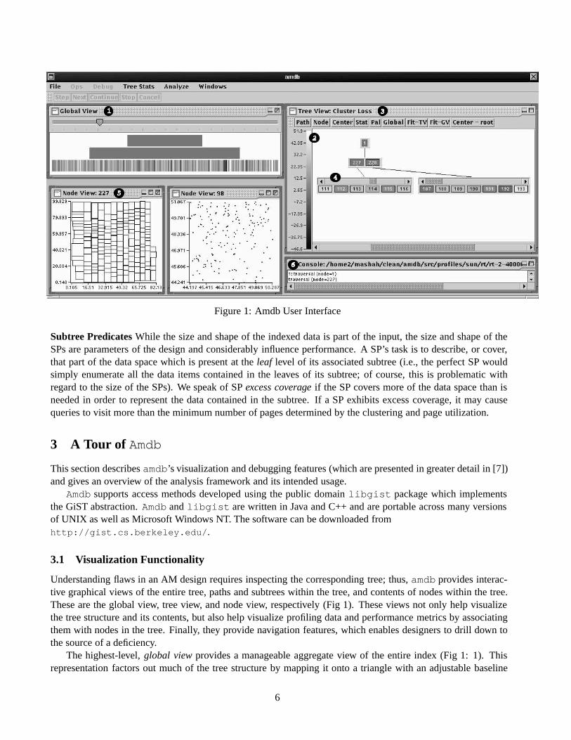
Figure 1: Amdb User Interface

Subtree PredicatesWhile the size and shape of the indexed data is part of the input, the size and shape of theSPs are parameters of the design and considerably influence performance. A SP’s task is to describe, or cover,that part of the data space which is present at theleaf level of its associated subtree (i.e., the perfect SP wouldsimply enumerate all the data items contained in the leaves of its subtree; of course, this is problematic withregard to the size of the SPs). We speak of SPexcess coverage if the SP covers more of the data space than isneeded in order to represent the data contained in the subtree. If a SP exhibits excess coverage, it may causequeries to visit more than the minimum number of pages determined by the clustering and page utilization.

3 A Tour of Amdb

This section describesamdb’s visualization and debugging features (which are presented in greater detail in [7])and gives an overview of the analysis framework and its intended usage.

Amdb supports access methods developed using the public domainlibgist package which implementsthe GiST abstraction.Amdb andlibgist are written in Java and C++ and are portable across many versionsof UNIX as well as Microsoft Windows NT. The software can be downloaded fromhttp://gist.cs.berkeley.edu/.

3.1 Visualization Functionality

Understanding flaws in an AM design requires inspecting the corresponding tree; thus,amdb provides interac-tive graphical views of the entire tree, paths and subtrees within the tree, and contents of nodes within the tree.These are the global view, tree view, and node view, respectively (Fig 1). These views not only help visualizethe tree structure and its contents, but also help visualize profiling data and performance metrics by associatingthem with nodes in the tree. Finally, they provide navigation features, which enables designers to drill down tothe source of a deficiency.

The highest-level,global viewprovides a manageable aggregate view of the entire index (Fig 1: 1). Thisrepresentation factors out much of the tree structure by mapping it onto a triangle with an adjustable baseline

6

and height. The purpose of this view is to project a user-selected tree statistic or performance metric onto thisabstract display and depict the variation of the statistics across the total tree. The user can choose both a colormap (or palette, Fig 1: 2) and a statistic; the global view assigns colors to the statistical values and rendersthe nodes accordingly. Nodes are visually concatenated and merged if necessary with other nodes on the samelevel. Thus, the pixel density of nodes increases geometrically with the level. The user can also perform anapproximate drill-down into an area of interest by clicking on it. Subsequently, a path from the root node to anode in the neighborhood of the specified point will be shown in the tree view, a lower-level view which showsmore detail.

The tree viewshows the structure of the search tree (Fig 1: 3). It offers an intuitive point-and-click interfacefor browsing the tree while improving on conventional tree navigation interfaces which become cumbersome forhigh fanout trees. In this view, the tree’s nodes are represented by boxes and labeled with a unique number forreference. Each node is enclosed in a scrollable and stretchable container which displays its direct siblings. Thiscontainer (Fig 1: 4) allows users to focus on nodes of interest while bounding the amount of detail displayed.Any node can be expanded or contracted by clicking on it. When a node is expanded, the container holding itschildren is displayed below it with a line linking the two; when contracted, the entire subtree below the node isremoved. Like the global view, the tree view represents a user-selected tree statistic or performance metric bycoloring the nodes. With these features, a user can simultaneously focus on several paths and subtrees of interestwithout being overwhelmed by the width of the search tree.

After drilling down from the global view and tree view, the user can investigate the contents of specificnodes usingamdb’s node view (Fig 1: 5). Since tree nodes contain arbitrary user-defined predicates, the accessmethod designer must provide a module that displays the node given its contents. Currently,amdb contains asuite of modules that visualize two-dimensional projections of spatial data. The node view also allows the userto simulate a split (by calling thepickSplit()extension function) and visualize the results by separating the itemswith contrasting colors. In addition to user-defined data visualization,amdb provides a textual description ofthe keys, their sizes, and associated pointers.

3.2 Debugging Functionality

The behavior of an AM can be difficult to understand without being able to observe its mechanics. Previously,only standard programming language debugging tools were available for examininglibgist AMs. Becausethese tools are designed for analyzing low level actions, such as a single line of source code, they are cumbersomefor gaining an understanding of how search and update operations behave and interact with the tree.

Amdb allows a designer to single-step through tree search and update commands. Those commands generateevents for various node-oriented actions, such as node split, node traversal,etc., which permits users to step fromevent to event. Since manual stepping can become tedious,amdb also supports breakpoints. Breakpoints canbe defined on generic events, e. g., node update, or can be tied to a specific tree node, e.g., update of node227. When a breakpoint event is encountered, execution is suspended, and the user has an option to single-stepthrough events or continue until the next breakpoint. Additionally,amdb allows batch execution of commandsvia scripts so users can conveniently restore state.

3.3 Overview of the Analysis Framework

The goal of the analysis framework is to explain the observed performance of an AM running a user-suppliedworkload. The single ultimate performance number is the total execution time of the entire workload. This totaldepends on the number and nature of page accesses, the buffering policy and the CPU time spent examiningpages. For brevity, we concentrate on explaining observed page accesses; please see [6] for a discussion of theremaining components of the performance equation.

7

In Section 1 we mentioned the deficiencies of the current practice of reporting performance with aggregateI/O numbers or data-specific metrics. To be effective and universally applicable, an analysis framework shouldhave three properties: (1) the performance metrics should be data-independent and not be tailored to the seman-tics of a particular application domain, so that the analysis framework is applicable in the full generality of theGiST AM design framework; (2) the performance metrics must give an indication of the quality of measuredAM performance in terms of the optimization objective, i.e., minimization of I/Os; (3) the metrics should givethe designer an understanding of the causes of observed performance.

In order to ensure data-independence of the framework, the workload—a tree and a set of queries—is aninput parameter of the analysis and the metrics characterize the performance of an AM specifically in the contextof that workload. Also, the performance metrics directly characterize the observed performance of the workloadexecution, namely the page accesses. They are not stated in terms of data or query semantics, and are thereforedata-independent.

Instead of simply reporting the number of observed page accesses, a more meaningful performance metric isthe difference between the number of page accesses in the actual tree and the optimal tree; we call this differencetheperformance loss. The optimal tree is defined as minimizing the total number of page accesses over the entireworkload. In general terms, it is a tree where (a) the data is clustered into leaf nodes to maximize the co-locationof data that is co-retrieved, (b) the nodes in the tree are packed to the desired degree of utilization, and (c)the subtree predicates only guide the search algorithm to subtrees with query answers. While this hypotheticaltree cannot be automatically synthesized for use, having knowledge of the execution profile of the workload, inparticular the result sets of the queries, allows us to approximate the optimal tree relatively accurately. Morespecifically, property (a) can be efficiently approximated via hypergraph clustering [5], and properties (b) and(c) can be simulated while gathering idealized performance results. The details are presented in [6].

Knowing the magnitude of performance loss is a clear indication of the quality of an AM, expressed inthe units of the optimization objective, I/Os. Moreover, the performance loss shows the potential for perfor-mance improvement, which cannot necessarily be discovered even when comparing two competing AM de-signs using traditional performance metrics. We can compute aquery performance loss, which expresses thedifference in the number of I/Os of a query executed against the actual tree and the workload-optimal tree.Similarly, we can compute anode performance loss, which expresses a node’s contribution to query or ag-gregate workload performance loss. The analysis framework also defines a number of additionalimplementa-tion metricsthat characterize aspects of the AM implementation; we refer the reader to [6] for more details.

Optimal Clustering UtilizationExcess

Coverage

Total I/Os

Total Performance Loss(Excess I/Os)

Figure 2: Decomposition of observed I/Os on a per-query and per-node basis

Given a particular performance loss, we can furthersubdivide it to reflect the fundamental performance-relevant properties of GiST-based AMs, namely clus-tering, page utilization and excess coverage loss.Clus-tering lossspecifies the part of performance loss thatcan be attributed to the difference between workload-optimal and achieved (leaf-level1) clustering in the in-dex tree;utilization lossspecifies the part that is at-tributable to node utilization deviating from a target uti-lization; excess coverage loss specifies the part that isdue to accesses to leaf nodes that contain no relevantdata to a query. All of these subdivisions of perfor-

mance loss are also specified in I/Os—possibly fractions of I/Os; They are summarized in Figure 2. Such abreakdown of performance loss is more useful than aggregate numbers, because it helps the designer under-stand the nature of the loss and thereby provides more insight into the causes of observed performance. Thebreakdown of the node metrics in particular helps the designer identify anomalies in the tree structure.

1The reason this is restricted to leaf-level clustering is explained in [6].

8

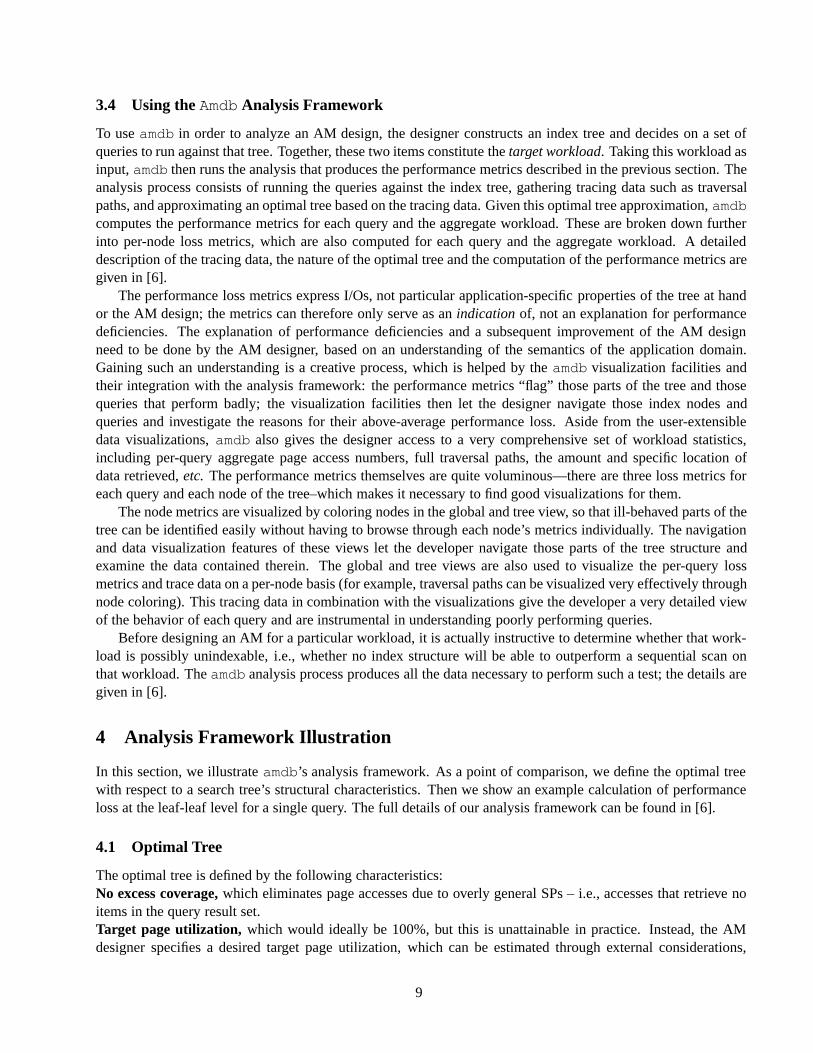
3.4 Using theAmdb Analysis Framework

To useamdb in order to analyze an AM design, the designer constructs an index tree and decides on a set ofqueries to run against that tree. Together, these two items constitute thetarget workload. Taking this workload asinput,amdb then runs the analysis that produces the performance metrics described in the previous section. Theanalysis process consists of running the queries against the index tree, gathering tracing data such as traversalpaths, and approximating an optimal tree based on the tracing data. Given this optimal tree approximation,amdbcomputes the performance metrics for each query and the aggregate workload. These are broken down furtherinto per-node loss metrics, which are also computed for each query and the aggregate workload. A detaileddescription of the tracing data, the nature of the optimal tree and the computation of the performance metrics aregiven in [6].

The performance loss metrics express I/Os, not particular application-specific properties of the tree at handor the AM design; the metrics can therefore only serve as anindicationof, not an explanation for performancedeficiencies. The explanation of performance deficiencies and a subsequent improvement of the AM designneed to be done by the AM designer, based on an understanding of the semantics of the application domain.Gaining such an understanding is a creative process, which is helped by theamdb visualization facilities andtheir integration with the analysis framework: the performance metrics “flag” those parts of the tree and thosequeries that perform badly; the visualization facilities then let the designer navigate those index nodes andqueries and investigate the reasons for their above-average performance loss. Aside from the user-extensibledata visualizations,amdb also gives the designer access to a very comprehensive set of workload statistics,including per-query aggregate page access numbers, full traversal paths, the amount and specific location ofdata retrieved,etc. The performance metrics themselves are quite voluminous—there are three loss metrics foreach query and each node of the tree–which makes it necessary to find good visualizations for them.

The node metrics are visualized by coloring nodes in the global and tree view, so that ill-behaved parts of thetree can be identified easily without having to browse through each node’s metrics individually. The navigationand data visualization features of these views let the developer navigate those parts of the tree structure andexamine the data contained therein. The global and tree views are also used to visualize the per-query lossmetrics and trace data on a per-node basis (for example, traversal paths can be visualized very effectively throughnode coloring). This tracing data in combination with the visualizations give the developer a very detailed viewof the behavior of each query and are instrumental in understanding poorly performing queries.

Before designing an AM for a particular workload, it is actually instructive to determine whether that work-load is possibly unindexable, i.e., whether no index structure will be able to outperform a sequential scan onthat workload. Theamdb analysis process produces all the data necessary to perform such a test; the details aregiven in [6].

4 Analysis Framework Illustration

In this section, we illustrateamdb’s analysis framework. As a point of comparison, we define the optimal treewith respect to a search tree’s structural characteristics. Then we show an example calculation of performanceloss at the leaf-leaf level for a single query. The full details of our analysis framework can be found in [6].

4.1 Optimal Tree

The optimal tree is defined by the following characteristics:No excess coverage,which eliminates page accesses due to overly general SPs – i.e., accesses that retrieve noitems in the query result set.Target page utilization, which would ideally be 100%, but this is unattainable in practice. Instead, the AMdesigner specifies a desired target page utilization, which can be estimated through external considerations,

9

Actual Tree:

X XXXX

Optimal Clustering:

XXX XX

0

7

654

321

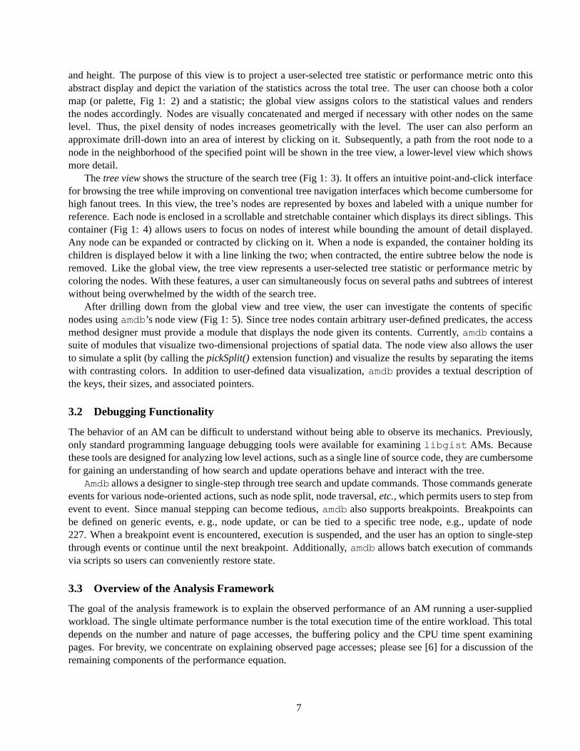
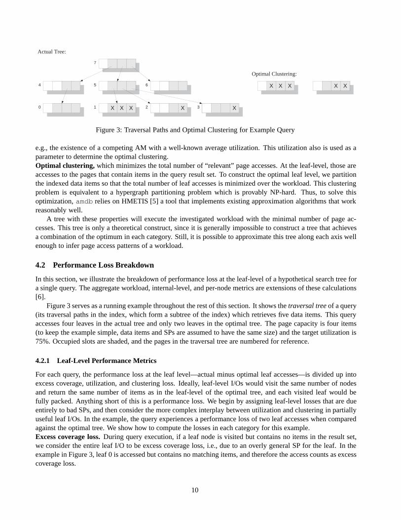
Figure 3: Traversal Paths and Optimal Clustering for Example Query

e.g., the existence of a competing AM with a well-known average utilization. This utilization also is used as aparameter to determine the optimal clustering.Optimal clustering, which minimizes the total number of “relevant” page accesses. At the leaf-level, those areaccesses to the pages that contain items in the query result set. To construct the optimal leaf level, we partitionthe indexed data items so that the total number of leaf accesses is minimized over the workload. This clusteringproblem is equivalent to a hypergraph partitioning problem which is provably NP-hard. Thus, to solve thisoptimization,amdb relies on HMETIS [5] a tool that implements existing approximation algorithms that workreasonably well.

A tree with these properties will execute the investigated workload with the minimal number of page ac-cesses. This tree is only a theoretical construct, since it is generally impossible to construct a tree that achievesa combination of the optimum in each category. Still, it is possible to approximate this tree along each axis wellenough to infer page access patterns of a workload.

4.2 Performance Loss Breakdown

In this section, we illustrate the breakdown of performance loss at the leaf-level of a hypothetical search tree fora single query. The aggregate workload, internal-level, and per-node metrics are extensions of these calculations[6].

Figure 3 serves as a running example throughout the rest of this section. It shows thetraversal treeof a query(its traversal paths in the index, which form a subtree of the index) which retrieves five data items. This queryaccesses four leaves in the actual tree and only two leaves in the optimal tree. The page capacity is four items(to keep the example simple, data items and SPs are assumed to have the same size) and the target utilization is75%. Occupied slots are shaded, and the pages in the traversal tree are numbered for reference.

4.2.1 Leaf-Level Performance Metrics

For each query, the performance loss at the leaf level—actual minus optimal leaf accesses—is divided up intoexcess coverage, utilization, and clustering loss. Ideally, leaf-level I/Os would visit the same number of nodesand return the same number of items as in the leaf-level of the optimal tree, and each visited leaf would befully packed. Anything short of this is a performance loss. We begin by assigning leaf-level losses that are dueentirely to bad SPs, and then consider the more complex interplay between utilization and clustering in partiallyuseful leaf I/Os. In the example, the query experiences a performance loss of two leaf accesses when comparedagainst the optimal tree. We show how to compute the losses in each category for this example.Excess coverage loss.During query execution, if a leaf node is visited but contains no items in the result set,we consider the entire leaf I/O to be excess coverage loss, i.e., due to an overly general SP for the leaf. In theexample in Figure 3, leaf 0 is accessed but contains no matching items, and therefore the access counts as excesscoverage loss.

10

Utilization loss. A leaf-level I/O that returns some useful items may contribute to performance loss in two ways.One way is through underfull leaf nodes. Deviation from the target utilization in the remaining leaves is summedup as utilization loss. In the example, leaf 2 has a utilization of 50%, which is2/3 of the target utilization of75%, resulting in a loss of1 − 0.5/0.75 = 1/3. The idea behind this accounting is that if the pages had beenpacked more densely, part of the accesses could have been avoided. Note that a page utilization in excess of thetarget utilization counts as a negative performance loss, i.e., a performance gain.Clustering loss. Once we have factored away any utilization loss, the remaining I/Os reflect the performanceof a ”tightly packed” leaf level. Clustering loss is the difference between the conceptually tightly packed leavesin the index and the corresponding leaves in the optimal tree. In the example, the result set is spread over threeleaves, or8/3 tightly packed leaves. The difference between that and the two leaf accesses in the optimal tree is2/3, the clustering loss.

To summarize the leaf-level metrics established for the example query: excess coverage loss is one I/O,utilization loss is1/3 I/Os and clustering loss2/3 I/Os. The sum is two I/Os, which is the total performanceloss that the example query experiences at the leaf level.

5 Conclusion

Amdb’s analysis facilities, in concert with its visualization features, are an invaluable tool for understanding theperformance characteristics of an AM and pinpointing the causes of deficiences. The analysis framework pro-vides a breakdown of an AM workload’s performance along three axes relevant to tree-based AMs: clustering,utilization, and the quality of subtree predicates. For each of these categories,amdb reports a performance lossin I/Os using an approximation to a workload- optimal tree as the basis for comparison. Such a breakdownprovides a better characterization of AM performance than aggregate numbers and is universally applicable toany AM design based on the GiST abstraction. In [6] we detail how these metrics are computed for an aggregateworkload as well as on a per-node and per-query basis, and we illustrate the use of these metrics on traditionalAMs. Amdb has been instrumental in several experimental design projects for improving the performance oftraditional AMs for specific applications [8, 9]. In [6] we highlight experiences in optimizing bulk-loaded R-trees for content-based image retrieval tasks, and summarize a user study in which a graduate database class wasasked to improve the performance of AMs on a synthetic dataset.

References

[1] P. Aoki. Generalizing “Search” in Generalized Search Trees (Extended Abstract). InProc. 14th ICDE, 1998.

[2] D. Comer. The Ubiquitous B-Tree.ACM Computing Surveys, 11(4):121–137, 1979.

[3] A. Guttman. R-Trees: A Dynamic Index Structure for Spatial Searching. InProc. ACM SIGMOD Conf., 1984.

[4] J. Hellerstein, J. Naughton, and A. Pfeffer. Generalized Search Trees for Database Systems. InProc. 21st VLDB,1995.

[5] G. Karypis, R. Aggarwal, V. Kumar, and S. Shekhar. Multilevel Hypergraph Partitioning: Applications in VLSIDomain. InProc. ACM/IEEE 34th Design Automation Conference, 1997.

[6] M. Kornacker, M. Shah, and J. Hellerstein. Amdb: A Design Tool for Access Methods. Technical Report UCB//CSD-03-1243, University of California at Berkeley, 2003.

[7] M. Shah, M. Kornacker, and J. Hellerstein. Amdb: A Visual Access Method Development Tool InUser Interfaces toData Intensive Systems, Edinburgh, UK, 1999.

[8] M. Thomas, C. Carson, and J. Hellerstein. Creating Customized Access Methods for Blobworld InProc. 16th ICDE,2000.

[9] M. Thomas and J. Hellerstein. Boolean Bounding Predicates for Spatial Access Methods InProc. DEXA, 2002.

11

A Status Report on XXL—a Software Infrastructure for EfficientQuery Processing

Michael Cammert, Christoph Heinz, Jürgen Kramer, Martin Schneider, Bernhard SeegerDepartment of Mathematics and Computer Science, University of Marburg, Germany

http://www.mathematik.uni-marburg.de/DBS/xxl

Abstract

XXL is a Java library that contains a rich infrastructure for implementing advanced query processingfunctionality. The library offers low-level components like access to raw disks as well as high-levelones like a query optimizer. On the intermediate levels, XXL provides a demand-driven cursor algebra,a framework for indexing and a powerful package for supporting aggregation. The library is publiclyavailable under GNU LGPL and comes with a full documentation.

1 Introduction

This paper describes the most important components of XXL, the eXtensible and fleXible Library for efficientquery processing [1, 2, 3]. Multiple reasons have driven the design and implementation of the library:

• Many of the algorithms developed for query processing have been implemented in an ad-hoc manner. Thesoftware design of these algorithms is poor and therefore, their application is quite complicated and limitedto specific (operating) systems. Furthermore, the modification of existing code is more complicated sincethe documentation is often not complete or even not available.

• XXL should support experimental evaluations within a uniform testbed that is freely available. It is dif-ficult to compare two access methods, for example, when the underlying platform is not the same. Theusage of different programming languages and compilers already results in substantial differences in theruntime. Consequently, most of the comparisons are based on a simplistic computing model where thenumber of I/Os is the only criterion.

• A more ambitious goal has been that XXL could serve as a repository for algorithms and use-cases. Werecognized that many algorithms are published in papers, but only a few implementations are freely avail-able. Wouldn’t it be great to have a collection of algorithms implemented under a uniform framework? Atleast in our research group, XXL has served as a repository where the code of our most important researchresults is transparently present.

The XXL project started four years ago. One of our first design decisions implied to use Java as the underly-ing programming language. With respect to our goals mentioned above, we were convinced that the advantages


12

of Java will outweigh its disadvantages. In particular, XXL benefits from the rich functionality available in otherJava libraries like the API of the SDK [4] and Colt [5]. We also agreed that the design of the library should bebased on popular design patterns [6]. This improves the readability and reusability of the code, and leads to acomprehensive documentation. XXL uses design patterns like factory, iterator and decorator. In order to im-prove code reusability, functional concepts had a strong influence on the design of the library. Java’s anonymousclasses are an excellent mechanism to provide functional abstraction in Java with very little overhead.

Another important aspect of our library is that classes should be well documented and equipped with use-cases. These are important for inexperienced users to get familiar with the mechanisms and the handling ofthe library. A simple use-case is therefore attached to every class in its corresponding main method. For morecomplex application scenarios, we also provide use-cases in separate classes.

The rest of the paper gives a brief outline of the functionality of XXL, placing emphasis on the new conceptsthat have been developed recently. In Section 2, we first provide an introduction of the basics like our functionalapproach, containers and cursors. The principles for query processing like indexing and join processing arepresented in Section 3. Another new important component is our native XML storage. In Section 4, advancedconcepts are presented where metadata has to be taken into account. In particular, we introduce our object-relational package and show how to provide query optimization within our library.

2 Basic Components

2.1 Functions and Predicates

Functional abstraction is a powerful mechanism for writing compact code. Since functions are not first classcitizens in Java, XXL provides the interfaceFunction which has to be implemented by a functional class. Anew functional object is declared at runtime using one of the following methods:

1. An anonymous class is implemented by extendingFunction and overriding a methodinvoke thatshould contain the executable code. An example for declaring a new function is given as follows:

Function maxComp = new Function() {public Object invoke (Object o1, Object o2) {return (((Comparable) o1).compareTo(o2) > 0) ? o1 : o2;

}}

2. The methodcompose of a functional object can be called to declare a new function by composition offunctional objects.

The code of a functional object is executed by calling the methodinvoke with the expected number of pa-rameters. Note that functional objects in XXL may have a status and therefore, are more powerful than puremathematical functions.

Due to its importance in database systems, we decided to provide a separate interface (Predicate) forBoolean functions. This improves the readability of the code as well as its performance since expensive castsare avoided. Relevant to databases are particularly predicates likeexist for specifying subqueries and thepredicates for supporting a three-value logic.

2.2 Containers

A container is an implementation of a map that provides an abstraction from the underlying physical storage.If an object is inserted into a container, a new ID is created and returned. An object of a container can only be

13

retrieved via the corresponding ID. Since a container is generally used for bridging the gap between levels of astorage hierarchy, mechanisms for buffer management are already included in a container.

There are many different implementations of containers in XXL. The classMapContainer refers to acontainer where the set of objects is kept in main memory. The purpose of this container is to run queries fastin memory and to support debugging. The classBlockFileContainer represents a file of blocks, wherea block refers to an array of bytes with a fixed length. This is for instance useful when index-structures likeR-trees are implemented.

Java does not support operations on binary data and therefore, a block has to be serialized into its objectrepresentation. Java’s serialization mechanism is however not appropriate since it has to be defined at compiletime. It is also too inflexible because there is only at most one serialization method for a class. XXL overcomesthese deficiencies by introducing the classConverterContainer that is a decorated container, i.e., an objectof this class is a container and consists of a container. In addition, this class provides a converter that transformsan object into a different representation. ABufferedContainer is also a decorator. Its primary task is tosupport object buffering in XXL.

In order to run experiments on external storage without interfering with the underlying operating systems,XXL contains classes that support access to raw devices. There are two possibilities:

1. The classNativeRawAccess offers native methods on a raw device. By usingNativeRawAccessthe classRawAccessRAF extends the classjava.io.RandomAccessFile, which is the storageinterface ofBlockFileContainer.

2. XXL offers an implementation of an entire file system that runs on a raw device. This is able to deliverfiles as objects of a class that extendsjava.io.RandomAccessFile. Therefore, an object of theclassBlockFileContainer can store its blocks in files of XXL’s file system.

2.3 Cursor

A cursor is an abstract mechanism to access objects within a stream. Cursors in XXL are independent from thespecific type of the underlying objects. The interface of a cursor is given by:

interface Cursor extends java.util.Iterator {Object peek();void update(Object o);void reset();void close();

}

A cursor extends the functionality of the iterator provided in the packagejava.util. Thepeek methodreports the next object of the iteration without changing the state of the iteration. A call ofreset sets thecursor to the beginning of the iteration. The methodclose stops the iteration and releases resources like filehandles. The methodupdate modifies the current object of the iteration.

XXL offers an algebra for processing cursors, i. e., there are a set of operations that require cursors as inputand return a cursor as output. We distinguish among three kinds of cursors:

• Input cursorsare wrappers for transforming a data source into a cursor. For example, XXL provides aninput cursor for transformingjava.sql.ResultSet into a cursor.

• Processing cursorsare the ones that modify the input cursor. Examples for such cursors areJoin,Grouper, Mapper whose semantics are similar to the ones of the corresponding relational operators.

• Flow cursorsdo not change the objects within the input stream, but they are restricted to change theunderlying data flow. For example, an instance of the classTeeCursor duplicates the input cursor.

14

3 Query Processing

3.1 Indexing

One of the most important packages of XXL isindexStructures that consists of a high-level frameworkfor index-structures. The purpose of this package is twofold: First, it contains many different index-structuresthat are ready-to-use. Second, the implementation of new ones should be simplified.

Let us give an example for using an index-structure like an M-tree [7]:

MTree mTree = new MTree(MTree.HYPERPLANE_SPLIT);mTree.initialize(getDescriptor, container, minCap, maxCap);

The first step is to call a constructor. In this example we used the one with a parameter where the split strategyis specified. The second step is an initialization of the M-tree. The first parametergetDescriptor refers toa functional object that computes a so-calleddescriptorfor a given data item. In case of the M-tree, a descriptorcorresponds to a bounding sphere. Our M-tree is able to manage any kind of objects as long as such a functionalobject is available. The next parameter is the container object which is responsible for managing the nodes of thetree. The other two parameters specify the minimum and maximum number of items within a node. Thereafter,the tree is ready for receiving operations like insertions and queries.

An implementation of a new index-structure requires a fundamental understanding of our framework that isa direct implementation of grow-and-post trees [8]. An index-structure is primarily determined by the inner classNode, which does not only describe the structure of the tree nodes, but also provides essential functionality forsplitting and searching. The main task when implementing a new index-structure is to code a specialized classfor the nodes. For example, a function is required to serialize a node of an index-structure. More details aboutthe implementation can be found in our Java sources [3], where B-trees are probably the best starting point.

3.2 Join Processing

Joins are among the most important operators in a database system. While relational systems basically rely onequi-joins, new applications like spatial databases require new types of join predicates. The goal of our joinprocessing framework was to provide a single implementation with the intention to support a bunch of differentjoin predicates efficiently. Furthermore, our framework is sufficiently generic to cover both sort-merge joins andhash-based joins. It keeps a small subset, a so-calledsweep-area, for each input source in main-memory wherethe join is processed on. Elements from the input are inserted into the associated sweep-area one by one. Afterthe insertion of an element, the other sweep-area is checked for join partners. A sweep-area can periodicallyreorganized to remove the elements not producing join results anymore.

The interfaceSweepArea is the top class of all sweep-areas in XXL. The most important functionalitylooks as follows:

public interface SweepArea {public void insert(Object o);public void reorganize(Object curStatus, int id);public Iterator query(Object o);...

}

The operations refer to the basic steps of join processing as described above. Note that every input has a uniqueidentifier which has to be specified when callingreorganize. There is a large number of different classesthat implement the interfaceSweepArea. We refer the interested reader to the documentation of XXL [3].

A join in XXL is called by the following statement:

Iterator it = new Join(input1, input2, HashBagSweepArea.FACTORY_METHOD,Tuplify.DEFAULT_INSTANCE);

15

The first two parameters refer to the two input sources. The third parameter is a factory method for creating asweep-area. In our example, the sweep-area is organized as a hash-table [15]. The last parameter is a functionalobject that specifies how to construct the output tuple of the join.

If a user of XXL is interested in implementing a new kind of join, she/he basically has to implement anappropriate class that satisfies the interfaceSweepArea. This is substantial easier than implementing a joinfrom scratch.

3.3 Aggregation

Aggregate operations are important in large database systems to deliver a quick overview of the response set.In contrast to a relational DBMS, XXL supports functions as results of aggregate operations. This allows re-turning a histogram or other more advanced statistical data structures directly to the user (without producing anintermediate relation). In the following, we briefly describe the basic structures of our packagestatistics.

This package is based on a generic aggregator cursor that applies a user-defined functions to aggregate theobjects of a given iterator. This cursor returns the intermediate value of the aggregate among the input that hasbeen consumed so far. The final value can be reported by a call toaggregator.last(), which consumes the entireiterator. An example of such an aggregator is given below:

Aggregator aggregator = new Aggregator(new RandomIntegers(100, 50),new Function () { // the aggregation function

public Object invoke (Object agg, Object next) {return (agg == null) ? next : maxComp.invoke(agg, next);

}}

);

In our example, the source consists of 50 random integers in the range [0,100). The anonymous function com-putes the maximum of two elements whereagg represents the aggregated value up to the previous element ofthe input andnext is the current element of the input.

Our statistics package provides different implementations of selectivity estimators with histograms and ker-nels as well as estimators based on query feedback. We refer the interested reader to our documentation [3], inorder to get more familiar with these concepts.

3.4 XML Storage

XXL contains functionality for processing queries on XML data. In addition to wrappers that transform XMLinput into Java objects, XXL also provides a class that implements native XML storage. A brief description ofthis class will be given in the following.

The native storage of XXL is an implementation of Natix [9] that performs quite similar to a B-tree. Thebasic idea is to keep adjacent nodes of an XML-object physically close to each other in one page of the tree, inorder to support insertions and updates efficiently. An insertion of an XML node first determines the page whereit has to be stored. This might result in an overflow of the page which then has to be split into two. This triggersa split of the XML document into smaller pieces which fit into pages.

4 Advanced Features

In this section, we present two packages of XXL that goes beyond the pure query processing techniques pre-sented so far. Both of these packages rely on the availability and maintenance of metadata, whereas the func-tionality is inherited from the core packages. In order to deliver metadata, a class has to satisfy the interface

16

MetaDataProvider that only offers the methodgetMetaData. The classMetaDataCursor combinesfor example the two interfacesMetaDataProvider andCursor.

Relational Connectivity XXL’s package relational offers the functionality for processing on object-relationaldata sources. The functionality of the package is similar to the one of cursors, but the operators are enhancedby the corresponding metadata. In addition, the operators are processing tuples rather than Java objects. Conse-quently, there are operators for join processing, grouping, projection,. . ..

An important functionality of this package is the availability of wrappers for transforming an object of theclassjava.sql.ResultSet into an object of classMetaDataCursor and vice versa. This enables us toprocess data from relational sources directly without storing them in a local database. Database systems likeCloudscape have increased the functionality of SQL by accepting cursors in the from-clause. This yields aneasy approach to extending the functionality of a database system. In [1], we presented an implementation of asimilarity join in Cloudscape using XXL’s join operator.

Query Optimization The recent version of XXL also includes a query optimizer for transforming relationaloperator trees into more efficient ones. In analogy to the optimizer of a DBMS, we first check for semanticallycorrectness of the operator tree. Then, the optimizer starts transforming the operator tree by using a set ofrules and a cost model. Eventually, the optimizer selects the specific algorithms for the implementation of theoperators.

Since our query optimizer is part of a library, we require metadata being attached to data sources, opera-tors, algorithms, functions and predicates. For operators, there are the interfacesOperatorInputMetaDataandOperatorOutputMetaData, which extend the functionality ofjava.sql.ResultSetMetaData.These interfaces include methods that estimate the selectivity of an underlying operator and its costs. Our func-tional metadata (FunctionMetaData) offer methods that specify the attributes of the input stream. Metadataon predicates also return an estimation of the predicate’s selectivity. Moreover, the algorithms considered in thephysical optimization step have to deliver metadata like the associated logical operator.

Important to the design of the optimizer was its extensibility and flexibility. In our architecture, it is easy toadd new predicates, operators and algorithms. Moreover, the underlying cost model is not fixed and might bereplaced by a different one. As an extra feature, we support an XML format for queries, i. e. operator trees canbe transformed into XML and vice versa.

5 Related Work

There has been only little work on the design and development of query processing libraries in the database liter-ature up to date. Most of the work published in the database community presents a system-oriented architecture.

Our work has been largely inspired by the pioneering work of Graefe and his Volcano system [10]. Both,Volcano and XXL, use a tree-structured query evaluation strategy, represented by algebra expressions, that isused to execute queries by demand-driven dataflows. Volcano already used so-calledsupport functionsformanipulating individual data objects in the dataflow. XXL however goes beyond the functionality of Volcano.First, it offers a richer query processing infrastructure, many different index-structures and more support forstatistics. Second, XXL also contains wrappers for diverse data sources. Third, the object-oriented design ofXXL allows an easy extension of its functionality.

The work on GiST [11] is closely related to our indexing framework, but GiST is actually a system that istightly coupled with its storage system. The focus of GIST is only on index-structures, whereas other function-ality is missing. It is notable that the grid-file implementation [12] had already great abstraction mechanismslike iterators.

17

The design of libraries is more related to the area of algorithms and data structures, where libraries likeLEDA [13] are well known. The focus of LEDA is more on data structures for main memory rather than on themanagement of very large data sets. Many of the abstraction mechanisms like functional classes are not availablein LEDA. TPIE [14] is designed to assist programmers in writing high performance I/O-efficient programs.However, the operators of TPIE cannot pass data directly between each other, but have to use a temporarystorage area. In addition, TPIE does not represent a pure library, because it relies on a special memory managerfor organizing the physical memory. This also implies that TPIE is not platform independent.

6 Conclusions and Future Work

XXL is a query processing library implemented in Java that includes the most important ingredients for efficientquery processing. The design of the library was determined by two goals: the functionality of XXL should beextended easily and XXL should be flexible enough for being customized fast to specific problems. Due to itspowerful methods, XXL is also an excellent platform for experimental work. Coding of new algorithms anddata structures requires substantial less time than beginning from scratch.

XXL is a live project! We are currently working on improving our indexing framework and strive for arealization of a processing algebra on data streams.

Acknowledgements We are grateful for the great contributions of the other and previous members of thedatabase group to the current version of XXL. This work has been supported by the German Research Society(DFG) under SE 553/2-2 and SE 553/4-1.

References

[1] J. van den Bercken, B. Blohsfeld, J.-P. Dittrich, J. Krämer, T. Schäfer, M. Schneider, B. Seeger: XXL - A LibraryApproach to Supporting Efficient Implementations of Advanced Database Queries. VLDB Conf. 2001: 39-48

[2] J. van den Bercken, J.-P. Dittrich, B. Seeger: javax.XXL: A prototype for a Library of Query processing Algorithms.SIGMOD Conf. 2000: 588

[3] The XXL Project, http://www.mathematik.uni-marburg.de/dbs/xxl, 2003

[4] JavaTM 2 Platform, Standard Edition, v 1.4.1 API Specification, http://java.sun.com/j2se/1.4.1/docs/api/, 2002

[5] The Colt Distribution - Open Source Libraries for High Performance Scientific and Technical Computing in Java,http://hoschek.home.cern.ch/hoschek/colt/V1.0.3/doc/index.html, 2002

[6] E. Gamma, R. Helm, R. Johnson, J. Vlissides: Design Patterns: Elements of Reusable Object-Oriented Software,Addison Wesley. October 1994.

[7] P. Ciaccia, M. Patella, P. Zezula: M-tree: An Efficient Access Method for Similarity Search in Metric Spaces. VLDBConf. 1997: 426-435

[8] D. Lomet: Grow and Post Index Trees: Roles, Techniques and Future Potential. Proc. Symp. on Spatial Databases1991: 183-206

[9] T. Fiebig, S. Helmer, C.-C. Kanne, G. Moerkotte, J. Neumann, R. Schiele, T. Westmann: Natix: A TechnologyOverview. Web, Web-Services, and Database Systems 2002: 12-33

[10] G. Graefe: Volcano - An Extensible and Parallel Query Evaluation System. TKDE 6(1): 120-135 (1994)

[11] J. Hellerstein, J. Naughton, A. Pfeffer: Generalized Search Trees for Database Systems. VLDB Conf. 1995: 562-573

[12] K. Hinrichs: Implementation of the Grid File: Design Concepts and Experience. BIT 25(4): 569-592 (1985)

[13] K. Mehlhorn, S. Naher: LEDA: A Platform for Combinatorial and Geometric Computing. Cambridge UniversityPress 1999

[14] L. Arge, O. Procopiuc, J. Vitter: Implementing I/O-efficient Data Structures Using TPIE. ESA 2002: 88-100

[15] A. Wilschut, P. Apers: Dataflow Query Execution in a Parallel Main-Memory Environment. PDIS 1991: 68-77

18

Generating Traffic Data

Thomas BrinkhoffInstitute for Applied Photogrammetry and Geoinformatics

FH Oldenburg/Ostfriesland/Wilhelmshaven (University of Applied Sciences)Ofener Str. 16/19, D-26121 Oldenburg, Germany

http://www.fh-oow.de/institute/personen/brinkhoff/

Abstract

Experimental investigations of spatiotemporal algorithms and data structures demand for generatorsthat produce realistic data sets. Especially Location-Based Services (LBS) require the simulation oftraffic. In this case, the data sets consist of objects that move within a given infrastructure. In this paper,two different approaches—the Network-based Generator and the City Simulator—are reviewed. Bothgenerators for traffic data have a great deal in common, but are different in certain points. In addition,a short overview on projects using these generators is given.

1 Introduction

Comprehensible performance evaluations are one of the most important requirements in the field of spatiotem-poral algorithms and data structures. This demand covers the preparation and use of well-defined test dataand benchmarks enabling the systematic and comprehensible evaluation and comparison of data structures andalgorithms.

In experimental investigations,synthetic datafollowing statistical distributions as well asreal datafrom real-world applications are used as test data or as query sets. The use of synthetic data allows testing the behavior ofan algorithm or of a data structure under exactly specified conditions or in extreme situations. In addition, fortesting the scalability, synthetic data sets are often suitable. However, it is difficult to assess the performance ofreal applications by employing synthetic data. The use of real data tries to solve this problem. In this case, theselection of data is crucial. For non-experts it is often difficult to decide whether a data set reflects a “realistic”situation or not.

For testing spatiotemporal algorithms and data structures, moving objects are required. Such objects shouldmodel moving persons or driving vehicles. Especially for Location-Based Services, data sets are useful that sim-ulate traffic. One suitable approach for gettingtraffic dataconsists of (1) a definition of an infrastructure, whichrestricts the movement of the objects, and (2) the computation of the moving objects within this infrastructure.If the infrastructure models a real-world environment, such an approach can be understood as a simulation thatgenerates synthetic data on top of real data.

In the last few years, several generators for producing spatiotemporal data have been developed [10, 8,9, 11]. Section 2 of this paper presents two proposals that generate traffic data according to the approach


19

mentioned before: the Network-Based Generator by Thomas Brinkhoff and the City Simulator by J. Kaufman,J. Myllymaki, and J. Jackson from IBM. Section 3 gives a short overview on projects that make use of datagenerated by these generators. The paper concludes with a summary and some suggestions for future work.

2 Generators for Traffic Data

2.1 Network-based Generator by Brinkhoff

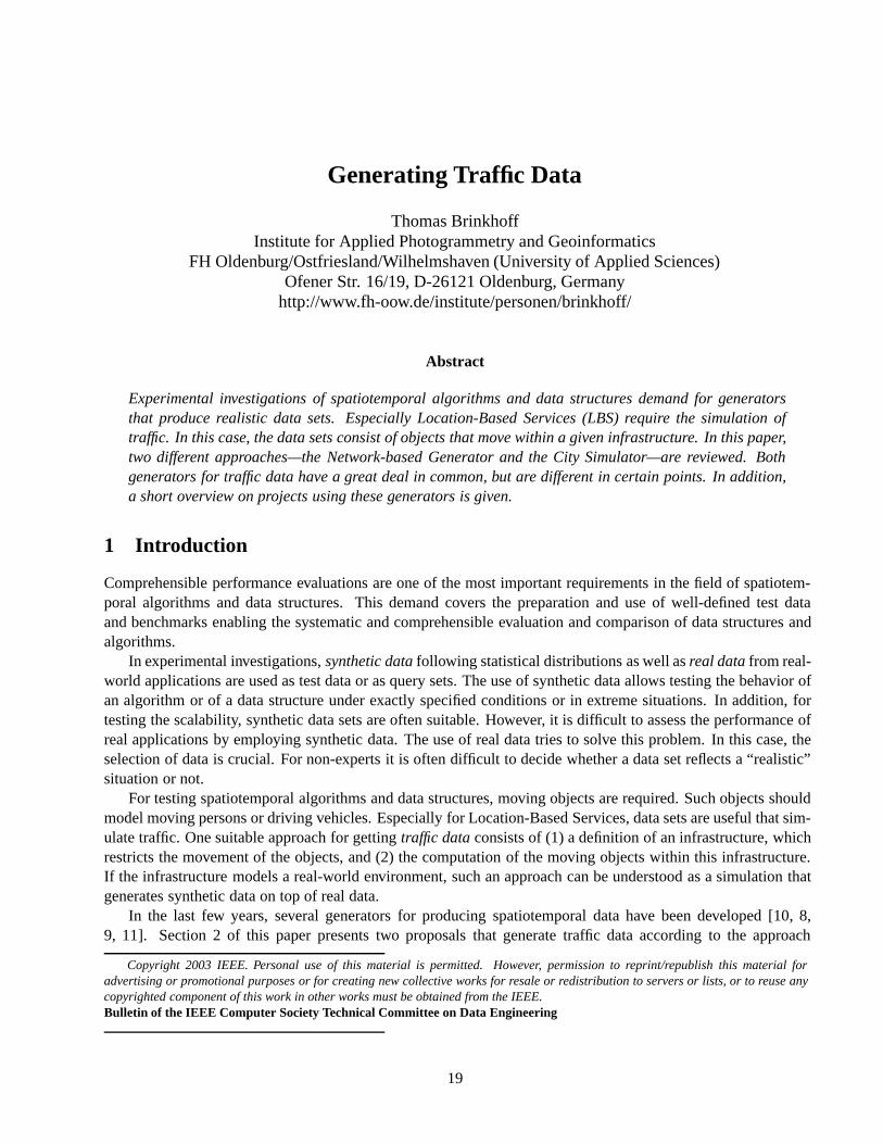
TheNetwork-based Generatorby Thomas Brinkhoff [1, 2] is based on the observation that objects often moveaccording to a network. This observation holds, e.g., for road traffic as well as for railway traffic. Air traffic alsofollows a network of air corridors and shipping is strongly influenced by rivers, channels, and other waterways.Herds of animals often follow a (invisible) network during their migration. In consequence, (almost) no objectscan be observed outside of the network. Figure 1 illustrates the graphical interface of the generator.

The generator uses a discrete time model: the whole period is divided byn time stamps. At each time stamp,new moving objects are generated and existing objects are moved or are deleted because they have reached theirdestination. Each moving object belongs to a class that specifies the behavior of the object. For example, the(maximum) speed is defined by such a class.

Figure 1: Visualization of the Network-based Generator.The points are the moving objects. The rectangles visual-ize the external objects. The colors indicate the classes ofroads, of moving objects, and of external objects.

Each edge of the network belongs to an edgeclass, which defines the speed limit and the capac-ity of an edge. If the number of objects travers-ing an edge at a time stamp exceeds the specifiedcapacity, the speed limit on this edge will be de-creased.

Furthermore, so-called external objects canbe generated in order to simulate the impact ofweather conditions or similar influences. There areexternal objects, which exist over the whole period,and others, which are created in the course of thesimulation and are deleted later. External objectsmay change their position and their (rectangular)shape over the time. If a moving object is in thecatchment area of an external object, its speed isinfluenced according to the parameters of the classthe external object belongs to.

The computations of the number of new objectsper time stamp, of the start location, of the lengthof a new route and of the location of the destina-tion are time-dependent. This feature allows mod-eling daily commuting and rush hours. In order tospeed up the computation, the route of an object iscomputed once at the time of its creation. How-ever, the fastest path may change over the time bythe motion of other objects and of external objects.Therefore, a re-computation is triggered by eventsdepending on the travel time (in order to simulatemessages of radio traffic services) and on the devi-

ation between the current speed and the expected speed on an edge (in order to simulate the reaction of driversin a traffic jam).

20

The Network-based Generator is written in Java 1.1. Its behavior can by influenced by a parameter file aswell as by extending or modifying a set of well-chosen Java classes that are provided as source code. A graphicaluser interface allows the setting of parameters and the visualization of the network and of the generated objects.

The network used by the generator is specified by simple text files or by spatial data stored in Oracle Spatial.The same holds for the output: the reported objects are written to a text file or into a database. The followingexample shows a selected part of such output file; each line consists of the type of event, the object ID, the classof the moving object, the index of the time stamp and the x,y coordinates:

newpoint 0 3 0 20435 19558point 0 3 1 20455 19688newpoint 5 0 1 13858 10979point 0 3 2 20475 19818point 5 0 2 13800 11627newpoint 10 1 2 5079 18012point 0 3 3 20496 19948point 5 0 3 13504 12223point 10 1 3 5334 17822newpoint 15 0 3 13566 20167disappearpoint 0 3 4 20493 20078point 5 0 4 13258 12841point 10 1 4 5981 17832point 15 0 4 13612 19876

The Network-based Generator can be downloaded from following web site:http://www.fh-oow.de/institute/iapg/personen/brinkhoff/generator.shtml

2.2 City Simulator by IBM

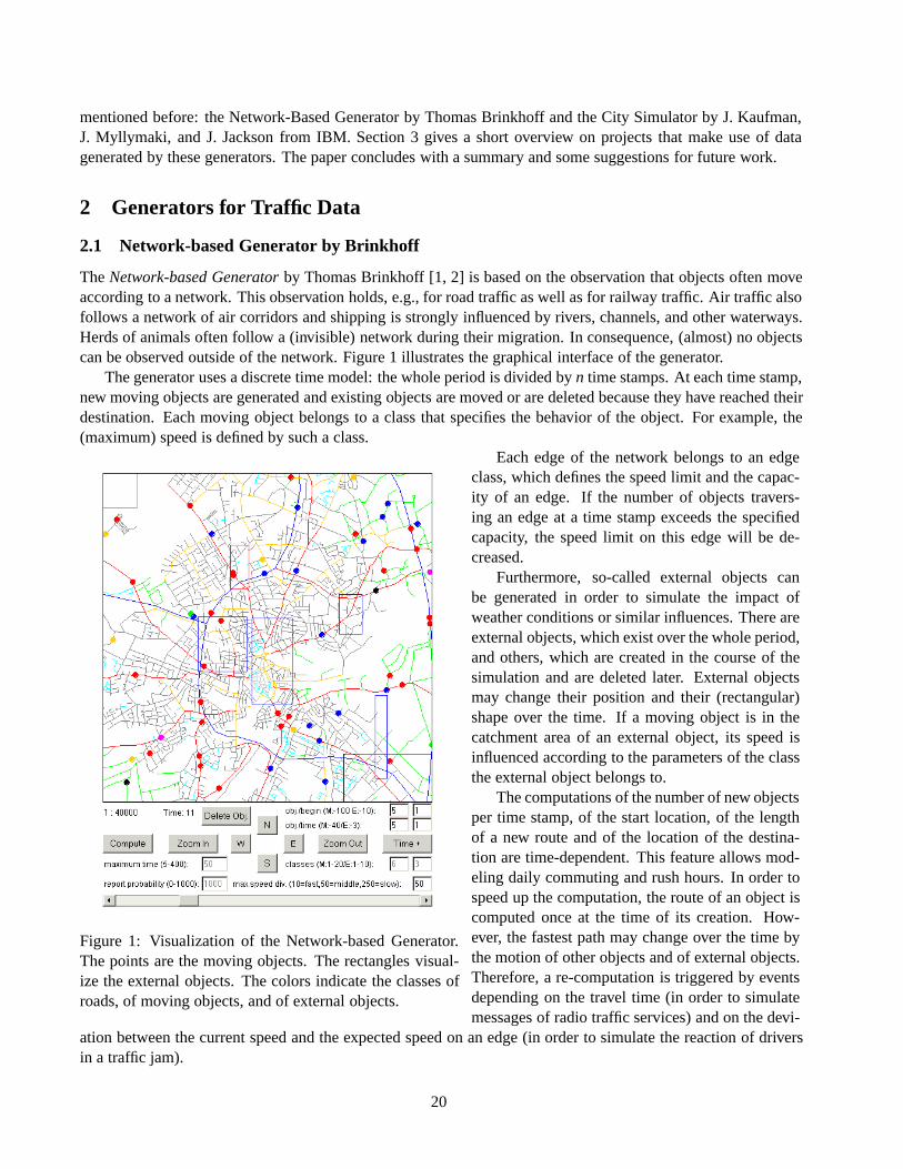
Figure 2: Visualization of a city plan.

The City Simulator by J. Kaufman, J. Myllymaki, andJ. Jackson [4, 5] is a scalable, three-dimensional model citythat enables the creation of dynamic spatial data simulatingthe motion of up to 1 million moving objects (persons). Thedata space of the city is divided into different types of placesthat influence the motion of the objects: roads, intersections,lawns and buildings are such places that define together acity plan. Each building consists of an individual number offloors for modeling the third dimension. Figure 2 illustratesa part of a city plan and the moving objects. The dark areasare buildings that are connected by a grid of roads. The smallpoints are moving objects; their colors indicate the currentfloor.

Moving objects being on a road enter with a user-definedprobability the first floor of a building. Objects on the firstfloor may leave the building if they are near a door. Theyperform random walks on a building floor or they may moveup or move down from one floor to the next floor depend-ing on user-defined probabilities if they are near to specificpoints (stairs). An object on a road moves with a linear com-bination of random walk and the drift velocity of the road;

the influence of the drift velocity increases as a moving object gets closer to the center of a road.

21

Figure 3: The floor population histogram visualizes the number of floors and the number of moving objects inrespect to a floor index.

The City Simulator is written in Java 2.0 using the Xerces class library. Several parameters allow controllingthe simulator. The number of objects and the number of time stamps are examples for such parameters. Theparameters are defined by a parameter file and may be re-defined by the input from a graphical user interface.Other parameters are defined by the city plan. The user interface allows the visualization of the city plan, of thegenerated objects, and of the number of objects being on the different floors (see Figure 3).

The output is produced as a text file, which contains a unique object ID, a time stamp, and x,y,z coordinates.The next example shows some selected lines such a file:

# index, time, x,y,z1, 4840.658295, 819.6,251.4,4.6 # cycle = 3201, 5266.601442, 817.2,247.8,0.0 # cycle = 3501, 5879.725107, 807.2,245.6,0.0 # cycle = 3901, 6176.540532, 804.2,249.0,4.6 # cycle = 4101, 6327.931518, 805.6,249.6,9.3 # cycle = 420

The city plan is described by an XML file. It contains information about geometries and about the probabil-ities of movements:

<Road Angle="0.0" Length="470.0" Width="100.0"><EndPoint1 x="0" y="1050"/><EndPoint2 x="470" y="1050"/><MotionRules EnterProb="0.1" ExitProb="0.1" VelGradient="2.4"/>

</Road><GrassyField Angle="0.0" Length="518.0" Width="506.0">

<EndPoint1 x="481" y="746"/><EndPoint2 x="999" y="746"/><MotionRules ExitProb="0.1"/>

</GrassyField><Building Angle="0.0" Length="518.0" Width="394.0">

<EndPoint1 x="481" y="1298"/><EndPoint2 x="999" y="1298"/><MotionRules ExitProb="0.1" UpProb="0.03"/><Floor Altitude="18" Angle="0" FloorNum="1" Length="518" Width="394">

<EndPoint1 x="481" y="1298"/><EndPoint2 x="999" y="1298"/>

22

<MotionRules DownProb="0.03" UpProb="0.03"/></Floor><Floor Altitude="36" Angle="0" FloorNum="2" Length="518" Width="394">

<EndPoint1 x="481" y="1298"/><EndPoint2 x="999" y="1298"/><MotionRules DownProb="0.03" UpProb="0.03"/>

</Floor></Building>

The Java class representing the city plan can be replaced by a user-specific class fulfilling a specified Javainterface. The download address of the City Simulator is:https://secure.alphaworks.ibm.com/aw.nsf/techs/citysimulator.

2.3 Discussion

Comparing both generators for traffic data, we can observe several similarities:

• A discrete time model is used.

• The generators are implemented in Java. Compiled class files are provided plus some source code.

• The infrastructure is specified by user-defined files.

• The motion of the objects is computed by a simulation.

• The output is produced as simple text files.

There are some significant differences: While the Network-based Generator is limited to two-dimensionaldata sets, the City Simulator supports three-dimensional city plans and computes 3D points. Another differenceconcerns the map: The first approach limits the movements of the objects by edges of width 0 whereas the CitySimulator defines areas. As a result, spatial clusters in the shape of lines can by expected by the Network-basedgenerator, and polygonal clusters using the City Simulator. In the case of the City Simulator, the movement ofthe objects is influenced by the rules of the place they are in. In contrast, the Network-based Generator alsoconsiders the possible influence of other moving objects.

3 Applications

This section gives a short overview on projects that are using the presented generators for traffic data.

LOCUS LOCUS [5] is a testbed for dynamic spatial indexing. It supports the DynaMark benchmark specifi-cation [6]. The City Simulator is a component of the architecture of LOCUS for generating location trace files.Each record in a location trace file is used for updating the spatiotemporal index. Aftern updates,mqueries likeproximity queries, k-nearest neighbor queries, and sorted-distance queries are executed in respect to the locationof a user. Figure 4 depicts the architecture of LOCUS.

MOX Applications tracking and presenting mobile objects require to be kept informed about new, relocated,or removed objects fulfilling a given query condition. Consequently, the spatiotemporal database system musttrigger its clients by transmitting the necessary information about such update operations. The query, whichcauses this process, is calledcontinuous query. MOX is an architecture for querying XML-represented movingobjects [3]. It especially supports continuous queries. Figure 5 illustrates the architecture of MOX. For testingthe system and for investigating continuous queries, the Network-based Generator has been integrated into MOX.The objects produced by the generator are inserted into the database, which triggers the affected continuousqueries.

23

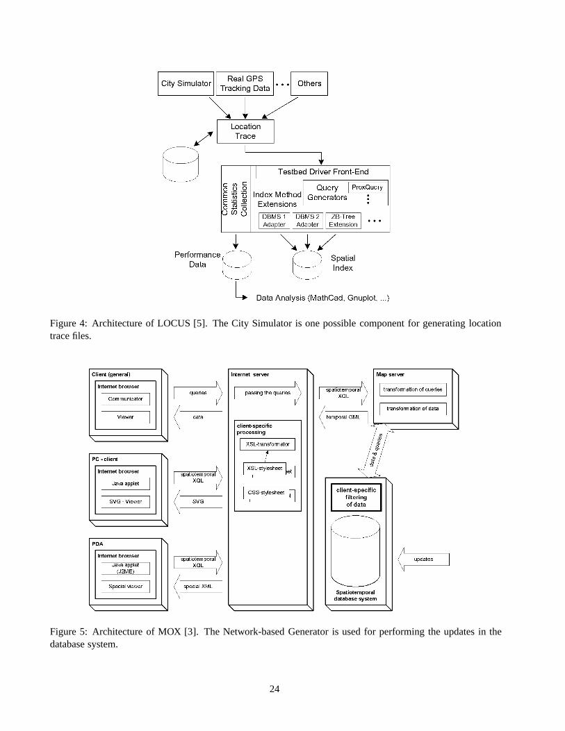
Figure 4: Architecture of LOCUS [5]. The City Simulator is one possible component for generating locationtrace files.

Figure 5: Architecture of MOX [3]. The Network-based Generator is used for performing the updates in thedatabase system.

24

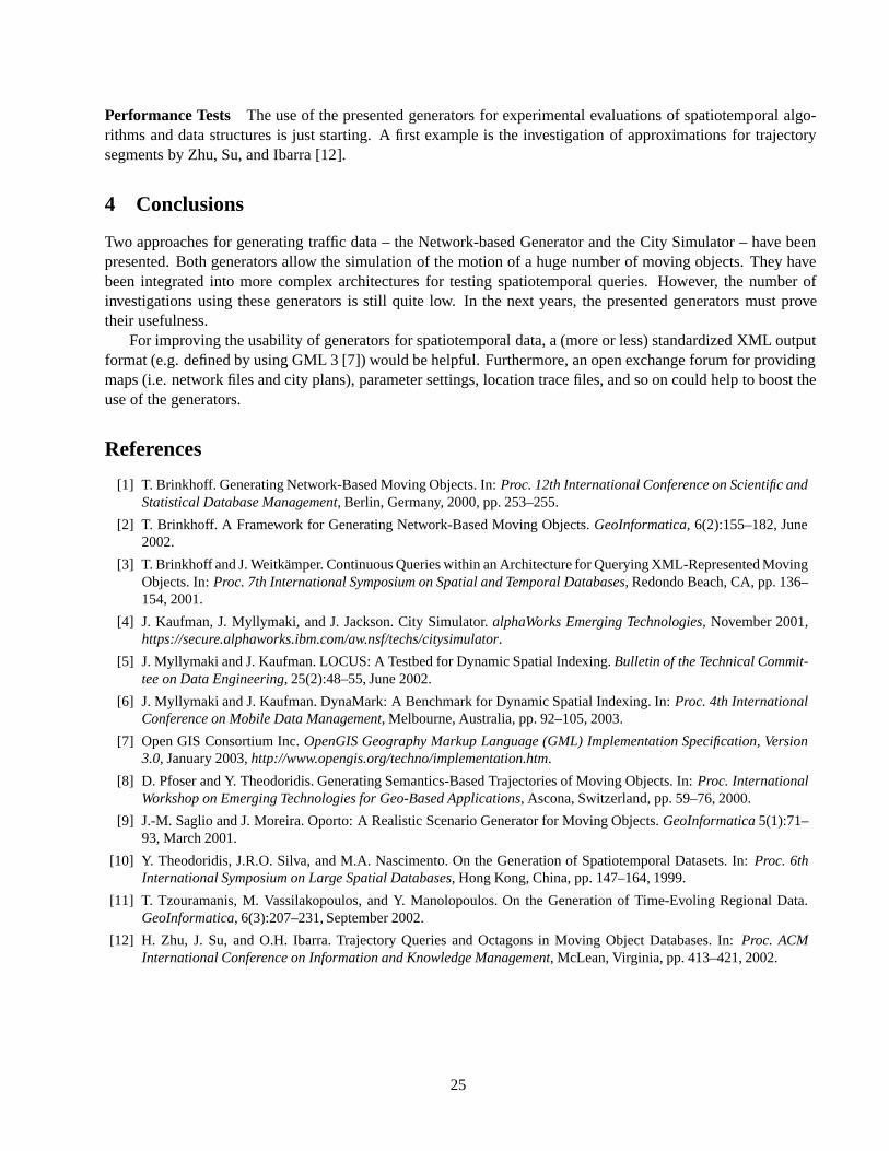
Performance Tests The use of the presented generators for experimental evaluations of spatiotemporal algo-rithms and data structures is just starting. A first example is the investigation of approximations for trajectorysegments by Zhu, Su, and Ibarra [12].

4 Conclusions

Two approaches for generating traffic data – the Network-based Generator and the City Simulator – have beenpresented. Both generators allow the simulation of the motion of a huge number of moving objects. They havebeen integrated into more complex architectures for testing spatiotemporal queries. However, the number ofinvestigations using these generators is still quite low. In the next years, the presented generators must provetheir usefulness.

For improving the usability of generators for spatiotemporal data, a (more or less) standardized XML outputformat (e.g. defined by using GML 3 [7]) would be helpful. Furthermore, an open exchange forum for providingmaps (i.e. network files and city plans), parameter settings, location trace files, and so on could help to boost theuse of the generators.

References

[1] T. Brinkhoff. Generating Network-Based Moving Objects. In:Proc. 12th International Conference on Scientific andStatistical Database Management, Berlin, Germany, 2000, pp. 253–255.

[2] T. Brinkhoff. A Framework for Generating Network-Based Moving Objects.GeoInformatica, 6(2):155–182, June2002.

[3] T. Brinkhoff and J. Weitkamper. Continuous Queries within an Architecture for Querying XML-Represented MovingObjects. In:Proc. 7th International Symposium on Spatial and Temporal Databases, Redondo Beach, CA, pp. 136–154, 2001.

[4] J. Kaufman, J. Myllymaki, and J. Jackson. City Simulator.alphaWorks Emerging Technologies, November 2001,https://secure.alphaworks.ibm.com/aw.nsf/techs/citysimulator.

[5] J. Myllymaki and J. Kaufman. LOCUS: A Testbed for Dynamic Spatial Indexing.Bulletin of the Technical Commit-tee on Data Engineering, 25(2):48–55, June 2002.

[6] J. Myllymaki and J. Kaufman. DynaMark: A Benchmark for Dynamic Spatial Indexing. In:Proc. 4th InternationalConference on Mobile Data Management, Melbourne, Australia, pp. 92–105, 2003.

[7] Open GIS Consortium Inc.OpenGIS Geography Markup Language (GML) Implementation Specification, Version3.0, January 2003,http://www.opengis.org/techno/implementation.htm.

[8] D. Pfoser and Y. Theodoridis. Generating Semantics-Based Trajectories of Moving Objects. In:Proc. InternationalWorkshop on Emerging Technologies for Geo-Based Applications, Ascona, Switzerland, pp. 59–76, 2000.

[9] J.-M. Saglio and J. Moreira. Oporto: A Realistic Scenario Generator for Moving Objects.GeoInformatica5(1):71–93, March 2001.

[10] Y. Theodoridis, J.R.O. Silva, and M.A. Nascimento. On the Generation of Spatiotemporal Datasets. In:Proc. 6thInternational Symposium on Large Spatial Databases, Hong Kong, China, pp. 147–164, 1999.

[11] T. Tzouramanis, M. Vassilakopoulos, and Y. Manolopoulos. On the Generation of Time-Evoling Regional Data.GeoInformatica, 6(3):207–231, September 2002.

[12] H. Zhu, J. Su, and O.H. Ibarra. Trajectory Queries and Octagons in Moving Object Databases. In:Proc. ACMInternational Conference on Information and Knowledge Management, McLean, Virginia, pp. 413–421, 2002.

25

Synthetic and Real Spatiotemporal Datasets

Mario A. Nascimento1 Dieter Pfoser2 Yannis Theodoridis3

1Department of Computing Science, University of Alberta, Canada,[email protected] Technology Institute, Greece,[email protected]

3Department of Informatics, University of Piraeus, Greece,[email protected]

Abstract

In the context of a spatiotemporal research environment, it is very important to be able to systematicallygenerate data with predictable characteristics. For instance, it allows one to use the same datasets, orothers similarly characterized, for benchmarking access structures or mining techniques. This paperpresents a survey of existing generators of synthetic spatiotemporal data. It also covers a few realdatasets, which are (at the time of this writing) publicly available for research use.

1 Introduction

While spatial data management and temporal management have been researched since more than 20 years ago(e.g., [6, 13]), the combination of both as a research topic is younger although just as strong in terms of interest(e.g., [7]).

Among the many topics which have been explored recently, such as spatiotemporal data modeling andquery languages (e.g., [5]), spatiotemporal data mining (e.g., [11]) and spatiotemporal indexing (e.g., [8]), many(notably the former two) require the use of datasets in order to be evaluated. Hence the need for an automaticmeans to generate datasets in a systematic way and with predictable characteristics. Interestingly, despite thesame need exists for “purely” spatial and temporal data, little work on data generation can be found, e.g., thea La Carteenvironment for benchmarking spatial joins (http://www.infres.enst.fr/˜bdtest/sigbench/) [4] and theSpyTimeenvironment for temporal data (http://www.cs.nyu.edu/cs/faculty/shasha/spytime/spytime.html).

Although we also cover some real spatiotemporal datasets, this paper deals mainly with the issue of gener-ating synthetic spatiotemporal data, with a focus on non-networked based data. (Network-based data generatorsare covered in [1] and elsewhere in this issue.) Towards this goal, the paper is structured as follows. Section 2covers GSTD, to our knowledge, the first web-based, spatiotemporal data generator and its enhancements overtime. Two other systems, G-TERD and Oporto are also reviewed, and all three are compared among themselves.Next, Section 3 presents some real datasets one could also use. Finally, we give directions for future work inSection 4.


26

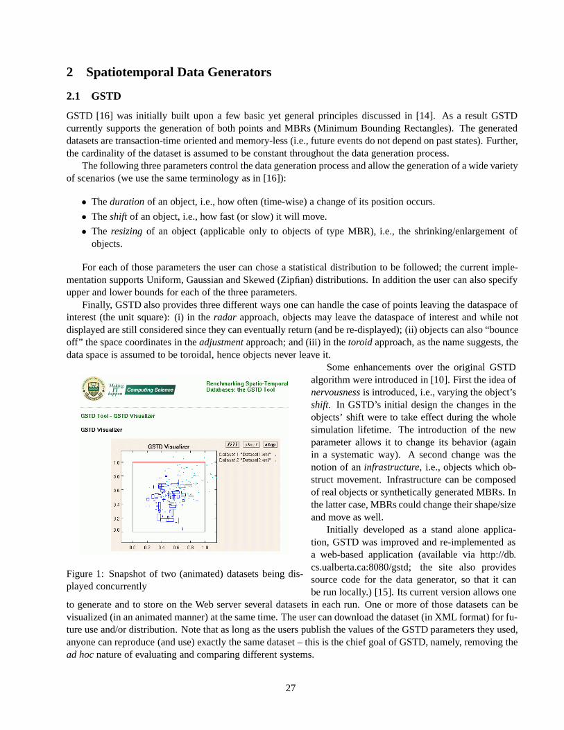
2 Spatiotemporal Data Generators

2.1 GSTD

GSTD [16] was initially built upon a few basic yet general principles discussed in [14]. As a result GSTDcurrently supports the generation of both points and MBRs (Minimum Bounding Rectangles). The generateddatasets are transaction-time oriented and memory-less (i.e., future events do not depend on past states). Further,the cardinality of the dataset is assumed to be constant throughout the data generation process.

The following three parameters control the data generation process and allow the generation of a wide varietyof scenarios (we use the same terminology as in [16]):

• Thedurationof an object, i.e., how often (time-wise) a change of its position occurs.

• Theshift of an object, i.e., how fast (or slow) it will move.

• The resizingof an object (applicable only to objects of type MBR), i.e., the shrinking/enlargement ofobjects.

For each of those parameters the user can chose a statistical distribution to be followed; the current imple-mentation supports Uniform, Gaussian and Skewed (Zipfian) distributions. In addition the user can also specifyupper and lower bounds for each of the three parameters.

Finally, GSTD also provides three different ways one can handle the case of points leaving the dataspace ofinterest (the unit square): (i) in theradar approach, objects may leave the dataspace of interest and while notdisplayed are still considered since they can eventually return (and be re-displayed); (ii) objects can also “bounceoff” the space coordinates in theadjustmentapproach; and (iii) in thetoroid approach, as the name suggests, thedata space is assumed to be toroidal, hence objects never leave it.

Figure 1: Snapshot of two (animated) datasets being dis-played concurrently

Some enhancements over the original GSTDalgorithm were introduced in [10]. First the idea ofnervousnessis introduced, i.e., varying the object’sshift. In GSTD’s initial design the changes in theobjects’ shift were to take effect during the wholesimulation lifetime. The introduction of the newparameter allows it to change its behavior (againin a systematic way). A second change was thenotion of aninfrastructure, i.e., objects which ob-struct movement. Infrastructure can be composedof real objects or synthetically generated MBRs. Inthe latter case, MBRs could change their shape/sizeand move as well.

Initially developed as a stand alone applica-tion, GSTD was improved and re-implemented asa web-based application (available via http://db.cs.ualberta.ca:8080/gstd; the site also providessource code for the data generator, so that it canbe run locally.) [15]. Its current version allows one

to generate and to store on the Web server several datasets in each run. One or more of those datasets can bevisualized (in an animated manner) at the same time. The user can download the dataset (in XML format) for fu-ture use and/or distribution. Note that as long as the users publish the values of the GSTD parameters they used,anyone can reproduce (and use) exactly the same dataset – this is the chief goal of GSTD, namely, removing thead hocnature of evaluating and comparing different systems.

27

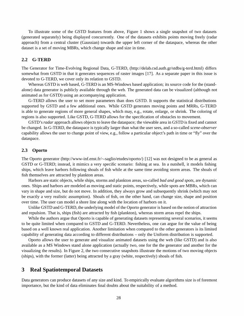
To illustrate some of the GSTD features from above, Figure 1 shows a single snapshot of two datasets(generated separately) being displayed concurrently. One of the datasets exhibits points moving freely (radarapproach) from a central cluster (Gaussian) towards the upper left corner of the dataspace, whereas the otherdataset is a set of moving MBRs, which change shape and size in time.

2.2 G-TERD

The Generator for Time-Evolving Regional Data, G-TERD, (http://delab.csd.auth.gr/stdbs/g-terd.html) differssomewhat from GSTD in that it generates sequences of raster images [17]. As a separate paper in this issue isdevoted to G-TERD, we cover only its relation to GSTD.

Whereas GSTD is web based, G-TERD is an MS-Windows based application; its source code for the (stand-alone) data generator is publicly available through the web. The generated data can be visualized (although notanimated as for GSTD) using an accompanying application.

G-TERD allows the user to set more parameters than does GSTD. It supports the statistical distributionssupported by GSTD and a few additional ones. While GSTD generates moving points and MRRs, G-TERDis able to generate regions of more general shapes, which may, e.g., rotate, enlarge, or shrink. The coloring ofregions is also supported. Like GSTD, G-TERD allows for the specification of obstacles to movement.

GSTD’sradar approach allows objects to leave the dataspace; the viewable area in GSTD is fixed and cannotbe changed. In G-TERD, the dataspace is typically larger than what the user sees, and a so-calledscene-observercapability allows the user to change point of view, e.g., follow a particular object’s path in time or “fly” over thedataspace.

2.3 Oporto

The Oporto generator (http://www-inf.enst.fr/∼saglio/etudes/oporto/) [12] was not designed to be as general asGSTD or G-TERD; instead, it mimics a very specific scenario: fishing at sea. In a nutshell, it models fishingships, which leave harbors following shoals of fish while at the same time avoiding storm areas. The shoals offish themselves are attracted by plankton areas.

Harbors are static objects, while ships, storms and plankton areas, so-calledbad and good spots, are dynamicones. Ships and harbors are modeled as moving and static points, respectively, while spots are MBRs, which canvary in shape and size, but do not move. In addition, they always grow and subsequently shrink (which may notbe exactly a very realistic assumption). Shoals of fish, on the other hand, can change size, shape and positionover time. The user can model a shore line along with the location of harbors on it.

Unlike GSTD and G-TERD, the underlying model of the Oporto generator is based on the notion of attractionand repulsion. That is, ships (fish) are attracted by fish (plankton), whereas storm areas repel the ships.

While the authors argue that Oporto is capable of generating datasets representing several scenarios, it seemsto be quite limited when compared to GSTD and G-TERD. Nevertheless, one can argue for the value of beingbased on a well known real application. Another limitation when compared to the other generators is its limitedcapability of generating data according to different distributions – only the Uniform distribution is supported.

Oporto allows the user to generate and visualize animated datasets using the web (like GSTD) and is alsoavailable as a MS Windows stand alone application (actually two, one for the the generator and another for thevisualizing the results). In Figure 2, the two consecutive snapshots illustrate the motions of two moving objects(ships), with the former (latter) being attracted by a gray (white, respectively) shoals of fish.

3 Real Spatiotemporal Datasets

Data generators can produce datasets of any size and kind. To empirically evaluate algorithms size is of foremostimportance, but the kind of data eliminates final doubts about the suitability of a method.

28

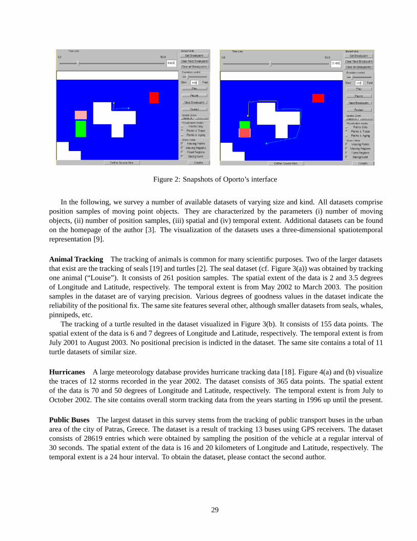
Figure 2: Snapshots of Oporto’s interface

In the following, we survey a number of available datasets of varying size and kind. All datasets compriseposition samples of moving point objects. They are characterized by the parameters (i) number of movingobjects, (ii) number of position samples, (iii) spatial and (iv) temporal extent. Additional datasets can be foundon the homepage of the author [3]. The visualization of the datasets uses a three-dimensional spatiotemporalrepresentation [9].

Animal Tracking The tracking of animals is common for many scientific purposes. Two of the larger datasetsthat exist are the tracking of seals [19] and turtles [2]. The seal dataset (cf. Figure 3(a)) was obtained by trackingone animal (“Louise”). It consists of 261 position samples. The spatial extent of the data is 2 and 3.5 degreesof Longitude and Latitude, respectively. The temporal extent is from May 2002 to March 2003. The positionsamples in the dataset are of varying precision. Various degrees of goodness values in the dataset indicate thereliability of the positional fix. The same site features several other, although smaller datasets from seals, whales,pinnipeds, etc.

The tracking of a turtle resulted in the dataset visualized in Figure 3(b). It consists of 155 data points. Thespatial extent of the data is 6 and 7 degrees of Longitude and Latitude, respectively. The temporal extent is fromJuly 2001 to August 2003. No positional precision is indicted in the dataset. The same site contains a total of 11turtle datasets of similar size.

Hurricanes A large meteorology database provides hurricane tracking data [18]. Figure 4(a) and (b) visualizethe traces of 12 storms recorded in the year 2002. The dataset consists of 365 data points. The spatial extentof the data is 70 and 50 degrees of Longitude and Latitude, respectively. The temporal extent is from July toOctober 2002. The site contains overall storm tracking data from the years starting in 1996 up until the present.

Public Buses The largest dataset in this survey stems from the tracking of public transport buses in the urbanarea of the city of Patras, Greece. The dataset is a result of tracking 13 buses using GPS receivers. The datasetconsists of 28619 entries which were obtained by sampling the position of the vehicle at a regular interval of30 seconds. The spatial extent of the data is 16 and 20 kilometers of Longitude and Latitude, respectively. Thetemporal extent is a 24 hour interval. To obtain the dataset, please contact the second author.

29

68.5 69 69.5 70 70.5 71 40

42

44

2.4

2.5

2.6

2.7

2.8

2.9

3

3.1

3.2

3.3

Latitude (North

Longitute (West)

Yea

r+20

00

(a) seal

81 82 83 84 85 86 87 88 20

30

40

1.6

1.8

2

2.2

2.4

2.6

2.8

3

Latitute (North)

Longitude (West)

Yea

r+20

00(b) turtle

Figure 3: Animal tracking datasets

−110 −100 −90 −80 −70 −60 −50 −40 −300

10

20

30

40

50

60

70

Longitude (West)

Latit

ude

(Nor

th)

(a) spatial projection

−120 −100 −80 −60 −40 −20 0

50

100

7

7.5

8

8.5

9

9.5

10

10.5

Latitude (North)

Longitude (West)

Mon

ths

in 2

002

(b) spatiotemporal representation

Figure 4: Hurricane dataset

30

2.92 2.94 2.96 2.98 3 3.02 3.04 3.06 3.08

x 105

4.224

4.226

4.228

4.23

4.232

4.234

4.236

4.238

4.24

4.242

4.244x 10

6

Longitude (meters)

Latit

ude

(met

ers)

(a) spatial projection

2.9 2.95 3 3.05 3.1

x 105

4.22

4.24

4.26

x 106

6

8

10

12

14

16

18

20

22

Latitude (meters)Longitude (meters)

Tim

e of

Day

(ho

urs)

(b) spatial projection

Figure 5: Bus dataset

4 Future Work

One clear shortcoming common to all of the above tools is that they can only generate 2D spatiotemporal data.Although one would not be able visualize the generated data, it would be useful (and not as intuitive) to be ableto generate datasets in higher dimensional spaces.

Such tools could be further improved to allow maintaining a (likely moderated) database of datasets gener-ated, specially those used in publications. Some published papers simply mention the use of those tools withoutspecifying details, which makes it hard (if not impossible) for someone to duplicate their datasets, defeating thevery purpose of such tools.

GSTD and Oporto could be extended to allow the user to import real datasets to serve as the data space’sinfrastructure (G-TERD does allow this) and/or allow the user to create those by sketching them in the interfaceitself. Another useful enhancement could be to have objects aware of each other, e.g., one cannot get closer (orfarther) than a predetermined distance. (Oporto allows this in the special case of objects belonging to differentclasses only.) Note that this would require some kind of embedded spatiotemporal indexing, which could be aplug-in method provided by the user him/herself.

Indexing trajectories seems to be a topic of growing interest, as such, the above tools could also be extendedto generate trajectories following some particular specification, e.g., be contained within a pre-defined corridor.

Acknowledgments The authors would like to thank and acknowledge the following people who took partin GSTD’s development over the past years: Jefferson R. O. Silva, Aggelos Kokorogiannis, Giannis Poulakis,Victor Salamon, and Daniel Mallett. The development of GSTD has been partially supported (at different timesand by different means) by: Chorochronos Project (European Union); FAPESP, CNPq and FINEP (Brazil); andTRC, NSRC and Nykredit Corp. (Denmark). M. A. Nascimento is currently supported by NSERC Canada. D.Pfoser’s research is supported in part by the Information Society Technologies programme of the European Com-mission, Future and Emerging Technologies under the IST-2001-32645 DBGlobe project, and the IXNILATHSproject funded by the Greek General Secretariat of Research and Technology. Y. Theodoridis is also with theData and Knowledge Engineering Group at the Computer Technology Institute, Greece ([email protected]).

31

References

[1] T. Brinkhoff. A framework for generating network-based moving objects.Geoinformatica, 6(2):153–180, 2002.

[2] Caribbean Conservation Corporation/Sea Turtle Survival League. Sea turtle activity data, Web site:http://www.cccturtle.org/sat3.htm, 2003.

[3] D. Pfoser. Spatiotemporal datasets, Web site: http://dke.cti.gr/people/pfoser/data.html, 2003.

[4] O. Guenther et al. Benchmarking spatial joinsa la carte. In Proc. of the 10th Intl. Conf. on Scientific and StatisticalDatabase Management, pages 32–41, 1998.

[5] R.H. Gueting et al. A foundation for representing and querying moving objects.ACM Trans. on Database Systems,25(1):1–42, 2001.

[6] A. Guttman. R-trees: A dynamic index structure for spatial searching. InProc. of 1994 ACM SIGMOD Intl. Conf.on Management of Data, pages 47–57, 1984.

[7] C.S. Jensen et al., editors.Proc. of the 7th Intl. Symp. on Advances in Spatial and Temporal Databases, volume 2121of Lecture Notes in Computer Science, 2001.

[8] G. Kollios et al. Indexing animated objects using spatiotemporal access methods.IEEE Trans. on Knowledge andData Engineering, 13(5):758–777, 2001.

[9] D. Pfoser and C. S. Jensen. Capturing the uncertainty of moving-object representations. InAdvances in SpatialDatabases, 6th International Symposium, SSD’99, Hong Kong, China, July 20-23, 1999, Proceedings, pages 111–132, 1999.

[10] D. Pfoser and Y. Theodoridis. Generating semantics-based trajectories of moving objects.Intl. J. of Computers,Environment and Urban Systems (Special issue on Emerging Technologies for Geo-Based Applications), 27(3):243–263, 2003.

[11] J.F. Roddick and K. Hornsby, editors.Proc. of the 1st Intl. Workshop on Temporal, Spatial, and Spatio-TemporalData Mining, volume 2007 ofLecture Notes in Computer Science, 2001.

[12] J.-M. Saglio and J. Moreira. Oporto: a realistic scenario generator for moving objects.Geoinformatica, 5(1):71–93,2001.

[13] R.T. Snodgrass and I. Ahn. Temporal databases.IEEE Computer, 19(3):35–42, 1986.

[14] Y. Theodoridis et al. Specifications for efficient indexing in spatiotemporal databases. InProc. of the 10th IEEE Intl.Conf. on Scientific and Statistical Database Management, pages 123–132, July 1998.

[15] Y. Theodoridis and M.A. Nascimento. Generating spatiotemporal datasets on the WWW.SIGMOD Record,29(3):39–43, 2000.

[16] Y. Theodoridis, J.R.O. Silva, and M.A. Nascimento. On the generation of spatiotemporal datasets. InProc. of the6th Intl. Symp. on Advances in Spatial Databases, pages 147–164, July 1999.

[17] T. Tzouramanis, M. Vassilakopoulos, and Y. Manolopoulos. On the generation of time-evolving regional data.Geoinformatica, 6(3):207–231, 2002.

[18] Unisys Weather. Atlantic hurricane data, Web site: http://weather.unisys.com/hurricane/index.html, 2003.

[19] WhaleNet. Satellite tagging data, maps and information, Web site: http://whale.wheelock.edu/whalenet-stuff/stopcover.html, 2003.

32

Generating Dynamic Raster Data

Theodoros Tzouramanis1 Michael Vassilakopoulos2 Yannis Manolopoulos1

1Dept. of Informatics, Aristotle University of Thessaloniki

541 24 Thessaloniki, GreeceE-mails:{theo,manolopo}@delab.csd.auth.gr

2Dept. of Informatics, Technological Educational Institute of Thessaloniki

P.O. Box 14561, 541 01 Thessaloniki, GreeceE-mail:[email protected]

Abstract

Benchmarking of spatio-temporal databases is an issue of growing importance. In case large real datasets are not available, benchmarking requires the generation of artificial data sets following the real-world behavior of spatial objects that change their locations, shapes and sizes over time. In this report,a generator for changing raster data, called “Generator of Time-Evolving Regional Data” (G-TERD),is presented. The basic concepts that determine the function of G-TERD are the structure of complextwo-dimensional raster objects, their color, maximum speed, zoom and rotation-angle per time slot, theinfluence of other moving or static objects on the speed and on the moving direction of an object, theposition and movement of the scene-observer, the statistical distribution of each changing factor andfinally, time. In the framework developed, the user can control the generator response by setting severalparameters values.

1 Introduction

Spatio-temporal databases(STDBs) provide a framework for the efficient storage and retrieval of all states of aspatial database over time. This includes the current and past states and the support of spatial queries that referto present and past time points, as well. During the last years many efforts have focused on spatio-temporalformalism, data models, query languages, visualization and access methods. However, little work has appearedon benchmarks for STDBs.

The goal of benchmarks in STDBs is to compare the performance of different implementation alterna-tives. An example of a benchmark is the comparison of space requirements and query execution time of spatio-temporal access methods (STAMs). In order to evaluate such STAMs, extensive experimentation using real andsynthetic data is required. A good benchmark must correspond to a recognizable, comprehensible real-life sit-uation. It is important that the results hold not only for a specific environment but in more general settings, aswell. Thus, the user is able to repeat the experiments and come to similar conclusions. Very often, either realdata sets are not available or they cannot be useful for testing extreme conditions. In both cases synthetic datasets can be generated by some artificial specifications rather than by obeying a real-world behavior.


33

Much work has been done towards data generation for benchmarks in prototype and commercial non-spatio-temporal databases (for example, [4, 5]). These generated data can be used to test different implementationsunder various operating conditions. In STDBs, the work on the generation of test data is limited and only a fewinnovative papers have appeared in the literature. In [9] the authors present a general approach for the generationof synthetic scenes of moving points, or rectangular objects. This approach is parameter-driven and does notsupport the interaction between objects. In [6], the previous work is extended by introducing new features to thegeneration process. In [7] a specialized spatio-temporal data generator, motivated by an application modelingfishing boats, is proposed, where there exist no, or very few restrictions for the motion: e.g., objects of one typemay be attracted, or repulsed by objects of other classes. Recently, another approach for the generation of testdata, which is motivated from applications in the context of traffic telematics, has been presented [1, 2].

None of these approaches is suitable for benchmarking STAMs for raster data (especially quadtree-basedSTAMs, for example, [11, 12]). In this report we review a novel approach for data generation, which is specif-ically designed for applications stemming from the field of dynamic (time-evolving) raster data [13]. The gen-erator presented in [13] is called“Generator of Time-Evolving Regional Data”(G-TERD). This software toolis highly parameterized so that different parameter values may produce spatio-temporal data set distributionswith different characteristics. In this framework, the user can control the behavior of the generator by definingparameters and statistical models. Such an approach considers the characteristics of a wide range of applications.

In order to make G-TERD available to the user for experimentation purposes, a Web site has been created,which allows downloading the MS-DOS executable file of the generator, the user documentation and the sourcecode in C language. The Web site is athttp://delab.csd.auth.gr/stdbs/g-terd.html and pro-vides, also, a visualization tool (based on Gnuplot 3.7) that runs under MS-Windows. It is offered with sampledata sets obeying different user-defined settings.

The remaining part of the report is organized as follows. Section 2 describes the basic concepts which wereconsidered during the generator design for continuously changing synthetic raster data. Section 3 describes theoperation of the new generator and some basic programming issues. Section 4 presents example setups and thesequences of scenes generated. Finally, the last section concludes the report and discusses future work issues.

2 Fundamental Concepts

We assume a two-dimensional workspace, where real coordinates are used (float numbers in C) and that thespace extent on the x- and the y-axis is set by the user. In the sequel, in order to simplify presentation, the valuesof coordinates are counted in “units”. With respect to the time domain, we assume that the changing scene lastsfor a period of timeT = [0, tmax). This period is divided in time slots. We further assume that the scene remainsunchanged during a time slot. In other words, time is digitized.

2.1 Objects and sub-objects

The basic data structure of G-TERD is thetime-evolving two-dimensional regional object. Each object consistsof a group of sub-objects which are quadrangles of the same, or different colors. This group of sub-objects, ingeneral, changes at each time slot. An object, or sub-object may have a static shape, or it can change its spatialextension with time. The spatial extension of an object is determined by the smallest possible two-dimensionalrectangle, calledMinimum Bounding Rectangle(MBR), that encloses all its sub-objects. The user sets themaximum size of the object MBR and the maximum size of the sub-object quadrangle.

In order to simulate real-world complex non-rectangular objects (e.g. cars, animals, airplanes, clouds, is-lands) by an object, some, or all of its sub-objects may be connected and remain connected, for the wholelifetime of the object.

The number of objects appearing in the scene and the number of sub-objects in an object are dynamic. The

34

objects may be static, or moving towards any spatial direction. The square sub-objects may, also, expand, orshrink and rotate around their center. For the sake of simplicity, both elastic shocks and plastic crushes betweenobjects, are not allowed. Instead, there is a possibility that the one object will pass over the other, as if there weremoving in different heights, or there is a possibility that both objects will change moving directions in order toavoid the crush.

2.2 The Scene-Observer

The scene-observerplays a central role in a time-evolving scene. In real-life, the observer may be a satellitemonitoring the earth surface, a telescope watching the space universe, the field of vision of a video or a photocamera, the eyes of an onlooker, etc. The scene-observer in G-TERD is a virtual two-dimensional rectangularwindow that shifts, zooms and rotates over the scene and films it, by printing one snapshot image per time slot,for the whole lifetime of the evolution.

The observer’s window side length is user-controlled and it digitizes a workspace portion. The dimensionsof a quadrangle of the workspace that is represented by a pixel of the observer’s window, or in other words, thesize of such a pixel varies according to the zoom-in, or zoom-out factor. The scene-observer may move towardsany spatial direction, or he/she may be static for some periods of time or for the whole scene lifetime. Theobserver may shift (“travel”) in a random way over the surface of the predefined workspace, or may follow themovement of a specific “live” object. Other functions supported are the zoom in-out and the rotation aroundthe center point of the observer’s window. Using the concept of the scene-observer’s window, a sequence ofmulticolored images that can be saved in the disk are produced.

2.3 Change of Spatial Locations, Size, Shape and Color of the Objects

Data objects may change their spatial location, size and/or their shape at different time intervals, according tothe values of their speed, zoom and rotation-angle fields. These fields are measured in units of the workspacecoordinate system per time slot and their domains are bounded by minimum and maximum values set by theuser. There are static, slow and fast moving objects. When an object is static (in slow movement) the speed,zoom and rotation of all its sub-objects is set at zero (at half the value of the speed, zoom and rotation of theobject). In real-life examples, objects appear gradually in our field of vision. This also holds for objects and sub-objects in G-TERD. Moreover, sub-ojects may have the same, different, or slightly different colors (followingchanges of the intensity of light).

3 The operation of G-TERD

3.1 User-Defined Parameters and Distributions

In G-TERD several parameters may be user-defined in order to let the user control the behavior of the generator(Table 1). The appropriate definition of these parameters is the simplest technique to control the properties ofthe resulting data sets. For instance, by settingspeed min = speed max for both the x- and y- axes, then allthe objects are forced to move in a parallel fashion at the same speed as if they were one object. This is similarto the movement of birds or military aircrafts flying together, or to the movement of a group of soldiers.

In order to have a generalized tool for benchmarking that simulates classes of real-life applications, severalquantities that determine the operation of this tool must be random variables that obey a specified distributionamong the ones mentioned above. For G-TERD, these random variables are presented in Table 2.

Through careful specification of different distributions for the variables of Table 2, the user can simulateseveral interesting scenarios. For instance, by using the exponential distribution with small mean for the speed

35

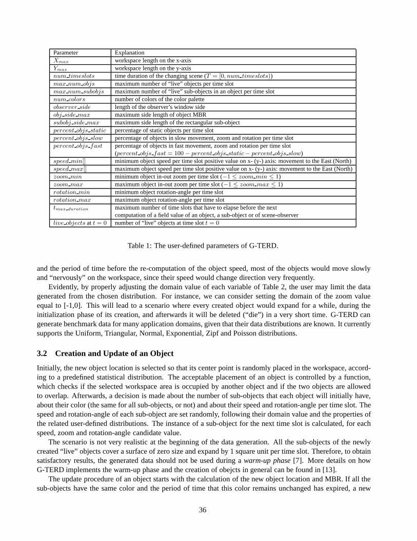
Parameter ExplanationXmax workspace length on the x-axisYmax workspace length on the y-axisnum timeslots time duration of the changing scene (T = [0, num timeslots))max num objs maximum number of “live” objects per time slotmax num subobjs maximum number of “live” sub-objects in an object per time slotnum colors number of colors of the color paletteobserver side length of the observer’s window sideobj side max maximum side length of object MBRsubobj side max maximum side length of the rectangular sub-objectpercent objs static percentage of static objects per time slotpercent objs slow percentage of objects in slow movement, zoom and rotation per time slotpercent objs fast percentage of objects in fast movement, zoom and rotation per time slot

(percent objs fast = 100 − percent objs static − percent objs slow)speed min[] minimum object speed per time slot positive value on x- (y-) axis: movement to the East (North)speed max[] maximum object speed per time slot positive value on x- (y-) axis: movement to the East (North)zoom min minimum object in-out zoom per time slot (−1 ≤ zoom min ≤ 1)zoom max maximum object in-out zoom per time slot (−1 ≤ zoom max ≤ 1)rotation min minimum object rotation-angle per time slotrotation max maximum object rotation-angle per time slottmax duration maximum number of time slots that have to elapse before the next

computation of a field value of an object, a sub-object or of scene-observerlive objects at t = 0 number of “live” objects at time slott = 0

Table 1: The user-defined parameters of G-TERD.

and the period of time before the re-computation of the object speed, most of the objects would move slowlyand “nervously” on the workspace, since their speed would change direction very frequently.

Evidently, by properly adjusting the domain value of each variable of Table 2, the user may limit the datagenerated from the chosen distribution. For instance, we can consider setting the domain of the zoom valueequal to [-1,0]. This will lead to a scenario where every created object would expand for a while, during theinitialization phase of its creation, and afterwards it will be deleted (“die”) in a very short time. G-TERD cangenerate benchmark data for many application domains, given that their data distributions are known. It currentlysupports the Uniform, Triangular, Normal, Exponential, Zipf and Poisson distributions.

3.2 Creation and Update of an Object

Initially, the new object location is selected so that its center point is randomly placed in the workspace, accord-ing to a predefined statistical distribution. The acceptable placement of an object is controlled by a function,which checks if the selected workspace area is occupied by another object and if the two objects are allowedto overlap. Afterwards, a decision is made about the number of sub-objects that each object will initially have,about their color (the same for all sub-objects, or not) and about their speed and rotation-angle per time slot. Thespeed and rotation-angle of each sub-object are set randomly, following their domain value and the properties ofthe related user-defined distributions. The instance of a sub-object for the next time slot is calculated, for eachspeed, zoom and rotation-angle candidate value.

The scenario is not very realistic at the beginning of the data generation. All the sub-objects of the newlycreated “live” objects cover a surface of zero size and expand by 1 square unit per time slot. Therefore, to obtainsatisfactory results, the generated data should not be used during awarm-up phase[7]. More details on howG-TERD implements the warm-up phase and the creation of obejcts in general can be found in [13].

The update procedure of an object starts with the calculation of the new object location and MBR. If all thesub-objects have the same color and the period of time that this color remains unchanged has expired, a new

36

Variable Distribution Domainnumber of “live” sub-objectsobj.live subobjs in user-defined [1, max num subobjs]an objectobj at the time slot of its creationinitial distribution of the center point of a new object user-defined the workspacenumber of new objects per time slot user-defined [0, max num objs − live objects]

number of new sub-objects in an object per time slot user-defined [0, max num subobjs − obj.live subobjs]

deletion time slotobj.endtime of an object user-defined [birth time of the object + 1,num timeslots]deletion time slotsubobj.endtime of a sub-object user-defined [birth time of the object in which

it belongs + 1,obj.endtime]color .color of an object or a sub-object user-defined [1, num colors]speedsubobj.speed of a moving user-defined [speed min, speed max]sub-object per time slot and spatial axiszoomsubobj.zoom of a moving sub-object per time slot user-defined [zoom min, zoom max]

with −1 ≤ zoom min ≤ zoom max ≤ 1

rotation-anglesubobj.rotation of user-defined [rotation min, rotation max]a moving sub-object per time slotnumber of time slots that must elapse before the next user-defined [1, tmax duration]computation of an attribute such as the speed, zoom, color, etc.

Table 2: Variables that are controlled by statistical distributions.

color for all its sub-objects is selected. Otherwise, each sub-object them may change its color, independently.If the period of time during which the speed, zoom and/or rotation-angle of each sub-object has expired, a newvalue is set to the corresponding field. The instance of the sub-object for the next time slot is calculated, for eachspeed, zoom and rotation-angle value and a procedure is followed to avoid an undesirable crush.

3.3 Positioning and Output of the Scene-Observer

The shift, zoom and rotation functions of the scene-observer are similar to the corresponding functions of anobject. If the scene-observer follows the evolution of a specific object, then the observer’s speed is proportionalto the distance of the center point of its window from the center point of the object followed. In this case, thezoom in-out function of the observer takes care of keeping the whole object inside the observer’s window.

The output of the scene-observer is a sequence of multicolored images that can be saved in the disk. Foreach pixel in the observer’s window, the algorithm checks if there is any sub-object covering the pixel. In thiscase, the sub-object color is recorded in the output. If sub-objects of different objects cover the same pixel of theobserver’s window, then the color of the object, which can pass over any other of the involved objects, appearsin the output image.

3.4 The Main Routine

The input of the algorithm consists of the values and statistical distributions of all the parameters and variablesthat appear in Table 1 and Table 2, respectively. During the scene initialization phase at time slott = 0, a user-defined number of “live” objects is created and located in the workspace. The initialization of the observer’swindow and the output of the first snapshot image of the time-evolving scene follow.

During the main loop phase new object instances are generated. If the deletion time slot of an object hasalready been reached and the surface of each of its sub-objects is less than 1 square unit, the object is deletedfrom the scene. A random number of new objects at each time slot is also created and placed in the workspace.The random number of new objects follows a predefined statistical distribution, such as the ones discussed insubsection 3.1. Finally, the observer’s window is located at another position over the workspace and the outputfunction prints the snapshot image of the current state of the continuously changing scene.

37

4 A Sample Run

In the following, we give an example of the use of G-TERD. The side length of the scene-observer’s windowis set at 1024 units, the maximum number of live objects per time slot is 70 and the lifetime of the evolution is101 time slots. The random number of new sub-objects per time slot and their deletion time slot are Uniform.The same holds for the speed, the color and the period of time that must elapse before the next computationof an attribute such as the speed, zoom, etc. Finally, the change of the size and shape of the objects/sub-objects are controlled by the zoom and rotation-angle values per time slot, which are generated by the Triangulardistribution. The scenario in Figure 1 illustrates static objects that are uniformly distributed in a workspace of

Figure 1: Static objects and a scene-observer moving from South-West to North-East.

2000× 2000 units (color versions of these greyscale figures can be obtained via the G-TERD site). The speeddomain value is [10,10] for each axis. Therefore, the scene-observer shifts over the workspace surface at aconstant speed and diagonal orientation, from South-West to North-East. The objects are all created at the initialtime slot, whereas in the sequel the creation of a new object is not allowed, since the distribution of new objectsper time slot was Normal with meanµ=0 and mean square deviationσ=0. No objects are deleted during thescene lifetime, since the distribution of their deletion time was also Normal with meanµ=100 and mean squaredeviationσ=0.

5 Conclusion and Future Work

In this report we reviewed the first approach, the G-TERD generator, for data generation specifically designedfor applications stemming from the field of dynamic (time-evolving) raster data. The basic concepts involved inthe development, operation and use of G-TERD were examined. G-TERD is highly parameterized and flexible,thus supporting the simulation of a variety of real-world scenarios. The Web site of G-TERD provides accessto the generator, its source code and some illustrative examples. G-TERD offers a framework for creating user-defined synthetic time-evolving raster data sets that can be used for the experimental comparison of differentSTAMs.

In the future, we plan enhancing G-TERD to support a greater variety of distributions, such as skeweddistributions or correlative two-dimensional distributions. Besides, the Web-based interface will be developedin order to both generate and make it possible to visualize time-evolving synthetic raster data.

38

References

[1] T. Brinkhoff: “Generating Network-Based Moving Objects,”Proc. 12th Int. Conf. on Scientific and StatisticalDatabase Management, pp.253-255, Berlin, Germany, 2000,

[2] T. Brinkhoff: “A Framework for Generating Network-Based Moving Objects,”Geoinformatica, Vol.6, No.2, pp.153-180, 2002

[3] O. Guenther, P. Picouet, J.-M. Saglio, M. Scholl and V. Oria: “Benchmarking Spatial Joins A La Carte,”Int. Journalof Geographical Information Science, Vol.13, No.7, pp.639-655, 1999.

[4] C. Gurret, Y. Manolopoulos, A. Papadopoulos and P. Rigaux: “BASIS: a Benchmarking Approach for Spatial IndexStructures,”Proc. Workshop on Spatiotemporal Database Management, pp.152-170, Edinburgh, Scotland, 1999.

[5] J. Pei, R. Mao, K. Hu and H. Zhu: “Towards Data Mining Benchmarking: a Testbed for Performance Study ofFrequent Pattern Mining,”Proc. 2000 ACM SIGMOD Conf., pp.592, Dallas, TX, 2000.

[6] D. Pfoser and Y. Theodoridis: “Generating Semantics-Based Trajectories of Moving Objects,”Proc. Workshop onEmerging Technologies for Geo-Based Applications, Ascona, Italy, 2000.

[7] J.-M. Saglio and J. Moreira: “Oporto: a Realistic Scenario Generator for Moving Objects,”Geoinformatica, Vol.5,No.1, pp.71-93, 2001.

[8] Y. Theodoridis and M.A. Nascimento: “Generating Spatiotemporal Datasets on the WWW,”ACM SIGMOD Record,Vol.29, No.3, pp.39-43, 2000.

[9] Y. Theodoridis, J.R.O. Silva and M.A. Nascimento: “On the Generation of Spatiotemporal Datasets,”Proc. 6th Symp.on Spatial Databases, pp.147-164, Hong Kong, China, 1999.

[10] Y. Theodoridis, T. Sellis, A. Papadopoulos and Y. Manolopoulos: “Specifications for Efficient Indexing in Spatiotem-poral Databases,”Proc. 7th Conf. on Statistical and Scientific Database Management Systems, pp.123-132, Capri,Italy, 1998.

[11] T. Tzouramanis, M. Vassilakopoulos and Y. Manolopoulos: “Multiversion Linear Quadtree for Spatio-TemporalData,”Proc. 4th East-European Conf. on Advanced Databases and Information Systems, pp.279-292, Prague, CzechRepublic, 2000.

[12] T. Tzouramanis, M. Vassilakopoulos and Y. Manolopoulos: “Overlapping Linear Quadtrees and Spatio-TemporalQuery Processing,”The Computer Journal, Vol.43, No.4, pp.325–343, 2000.

[13] T. Tzouramanis, M. Vassilakopoulos and Y. Manolopoulos: “On the Generation of Time-evolving Regional Data,”GeoInformatica, Vol.6, No.3, pp.207–231, 2002.

39

Spatio-Temporal Access Methods∗

Mohamed F. Mokbel Thanaa M. Ghanem Walid G. Aref

Department of Computer Sciences, Purdue University, West Lafayette, IN 47907-1398{mokbel,ghanemtm,aref}@cs.purdue.edu

Abstract

The rapid increase in spatio-temporal applications calls for new auxiliary indexing structures. A typicalspatio-temporal application is one that tracks the behavior of moving objects through location-awaredevices (e.g., GPS). Through the last decade, many spatio-temporal access methods are developed.Spatio-temporal access methods focus on two orthogonal directions: (1) Indexing the past, (2) Index-ing the current and predicted future positions. In this short survey, we classify spatio-temporal accessmethods for each direction based on their underlying structure with a brief discussion of future researchdirections.

1 Introduction

Spatio-temporal databases deal with objects that change their location and/or shape over time. A typical exampleof spatio-temporal databases is moving objects in theD-dimensional space. Moving objects learn about theirown location via location detection devices, e.g., GPS devices. Then, the objects report their locations to theserver using the underlying communication network, e.g., via wireless networks. The server stores the updatesfrom the moving objects and keeps a history of the spatio-temporal coordinates of each moving object. Inaddition, the server stores additional information to help predict the future positions of moving objects. Typicalqueries that are supported by such a server include time slice queries e.g., “Find all objects that cross a certainarea at time t” and window queries “Find all objects that cross a certain area in the time interval[t1, t2]”. Timeslice queries and window queries may ask about the past, current, or future times. Some queries are concernedonly with the past, e.g., trajectory queries “What is the maximum speed of a certain object in the last hour?”Other queries are concerned only with the future, e.g., moving window queries “Find the objects that intersecta moving area in a certain time interval”.

Numerous research have been done in developing spatio-temporal access methods as an auxiliary structureto support spatio-temporal queries. Figure 1 gives the evolution of spatio-temporal access methods with theunderlying spatial and temporal structures. Lines in the Figure indicate the relation between a new proposedspatio-temporal index structure and the original structure that is based upon.


∗This work was supported in part by the National Science Foundation under Grants IIS-0093116, EIA-9972883, IIS-0209120, andby Purdue Research Foundation.

40

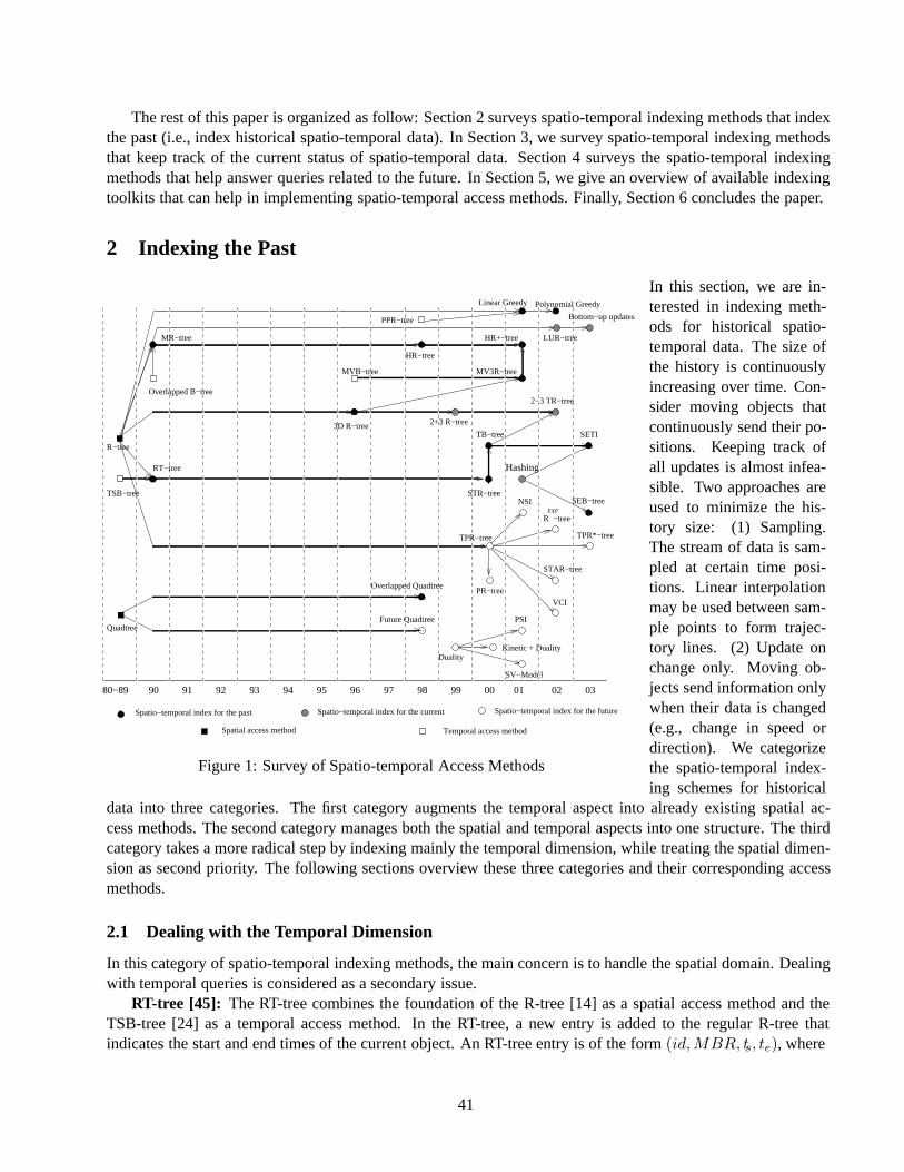
The rest of this paper is organized as follow: Section 2 surveys spatio-temporal indexing methods that indexthe past (i.e., index historical spatio-temporal data). In Section 3, we survey spatio-temporal indexing methodsthat keep track of the current status of spatio-temporal data. Section 4 surveys the spatio-temporal indexingmethods that help answer queries related to the future. In Section 5, we give an overview of available indexingtoolkits that can help in implementing spatio-temporal access methods. Finally, Section 6 concludes the paper.

2 Indexing the Past

90 91 92 93 94

2+3 R−tree

TB−tree

95 96 97 98 99 00 01 02 03

Hashing

80−89

2−3 TR−tree

STAR−tree

3D R−tree

Spatio−temporal index for the past Spatio−temporal index for the current Spatio−temporal index for the future

Spatial access method Temporal access method

SETI

SEB−tree

VCI

PR−tree

TPR−tree

Overlapped B−tree

HR−tree

Linear Greedy

Kinetic + Duality

SV−Model

PSI

Duality

NSISTR−tree

R −tree

TPR*−tree

MVB−tree

Overlapped Quadtree

Future Quadtree

EXP

HR+−tree

MV3R−tree

TSB−tree

RT−tree

Quadtree

R−tree

MR−tree

Polynomial Greedy

Bottom−up updates

LUR−tree

PPR−tree

Figure 1: Survey of Spatio-temporal Access Methods

In this section, we are in-terested in indexing meth-ods for historical spatio-temporal data. The size ofthe history is continuouslyincreasing over time. Con-sider moving objects thatcontinuously send their po-sitions. Keeping track ofall updates is almost infea-sible. Two approaches areused to minimize the his-tory size: (1) Sampling.The stream of data is sam-pled at certain time posi-tions. Linear interpolationmay be used between sam-ple points to form trajec-tory lines. (2) Update onchange only. Moving ob-jects send information onlywhen their data is changed(e.g., change in speed ordirection). We categorizethe spatio-temporal index-ing schemes for historical

data into three categories. The first category augments the temporal aspect into already existing spatial ac-cess methods. The second category manages both the spatial and temporal aspects into one structure. The thirdcategory takes a more radical step by indexing mainly the temporal dimension, while treating the spatial dimen-sion as second priority. The following sections overview these three categories and their corresponding accessmethods.

2.1 Dealing with the Temporal Dimension

In this category of spatio-temporal indexing methods, the main concern is to handle the spatial domain. Dealingwith temporal queries is considered as a secondary issue.

RT-tree [45]: The RT-tree combines the foundation of the R-tree [14] as a spatial access method and theTSB-tree [24] as a temporal access method. In the RT-tree, a new entry is added to the regular R-tree thatindicates the start and end times of the current object. An RT-tree entry is of the form(id,MBR, ts, te), where

41

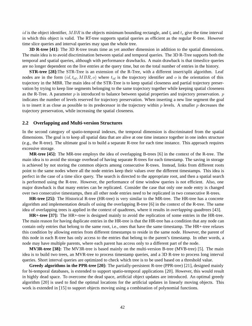
id is the object identifier,MBR is the objects minimum bounding rectangle, andts andte give the time intervalin which this object is valid. The RT-tree supports spatial queries as efficient as the regular R-tree. Howevertime slice queries and interval queries may span the whole tree.

3D R-tree [41]: The 3D R-tree treats time as yet another dimension in addition to the spatial dimensions.The main idea is to avoid discrimination between spatial and temporal queries. The 3D R-Tree supports both thetemporal and spatial queries, although with performance drawbacks. A main drawback is that timeslice queriesare no longer dependent on the live entries at the query time, but on the total number of entries in the history.

STR-tree [28]:The STR-Tree is an extension of the R-Tree, with a different insert/split algorithm. Leafnodes are in the form(id, tid,MBR, o) wheretid is the trajectory identifier ando is the orientation of thistrajectory in the MBR. The main idea of the STR-Tree is to keep spatial closeness and partial trajectory preser-vation by trying to keep line segments belonging to the same trajectory together while keeping spatial closenessas the R-Tree. A parameterp is introduced to balance between spatial properties and trajectory preservation.pindicates the number of levels reserved for trajectory preservation. When inserting a new line segment the goalis to insert it as close as possible to its predecessor in the trajectory withinp levels. A smallerp decreases thetrajectory preservation, while increasing the spatial closeness.

2.2 Overlapping and Multi-version Structures

In the second category of spatio-temporal indexes, the temporal dimension is discriminated from the spatialdimensions. The goal is to keep all spatial data that are alive at one time instance together in one index structure(e.g., the R-tree). The ultimate goal is to build a separate R-tree for each time instance. This approach requiresexcessive storage.

MR-tree [45]: The MR-tree employs the idea of overlapping B-trees [6] in the context of the R-tree. Themain idea is to avoid the storage overhead of having separate R-trees for each timestamp. The saving in storageis achieved by not storing the common objects among consecutive R-trees. Instead, links from different rootspoint to the same nodes where all the node entries keep their values over the different timestamps. This idea isperfect in the case of a time slice query. The search is directed to the appropriate root, and then a spatial searchis performed using the R-tree. However, the performance of time window queries is not efficient. Also, onemajor drawback is that many entries can be replicated. Consider the case that only one node entry is changedover two consecutive timestamps, then all other node entries need to be replicated in two consecutive R-trees.

HR-tree [25]: The Historical R-tree (HR-tree) is very similar to the MR-tree. The HR-tree has a concretealgorithm and implementation details of using the overlapping B-tree [6] in the context of the R-tree. The sameidea of overlapping trees is applied in the context of quadtrees, where it results inoverlapping quadtrees[43].

HR+-tree [37]: The HR+-tree is designed mainly to avoid the replication of some entries in the HR-tree.The main reason for having duplicate entries in the HR-tree is that the HR-tree has a condition that any node cancontain only entries that belong to the same root, i.e., ones that have the same timestamp. The HR+-tree relaxesthis condition by allowing entries from different timestamps to reside in the same node. However, the parent ofthis node in each R-tree has only access to the entries that belong to the parent’s timestamp. In other words, anode may have multiple parents, where each parent has access only to a different part of the node.

MV3R-tree [38]: The MV3R-tree is based mainly on the multi-version B-tree (MVB-tree) [5]. The mainidea is to build two trees, an MVR-tree to process timestamp queries, and a 3D R-tree to process long intervalqueries. Short interval queries are optimized to check which tree is to be used based on a threshold value.

Greedy algorithms in the PPR-tree [20]:The partially-persistent R-tree (PPR-tree) [21], designed mainlyfor bi-temporal databases, is extended to support spatio-temporal applications [20]. However, this would resultin highly dead space. To overcome the dead space, artificial object updates are introduced. An optimal greedyalgorithm [20] is used to find the optimal locations for the artificial updates in linearly moving objects. Thiswork is extended in [15] to support objects moving using a combination of polynomial functions.

42

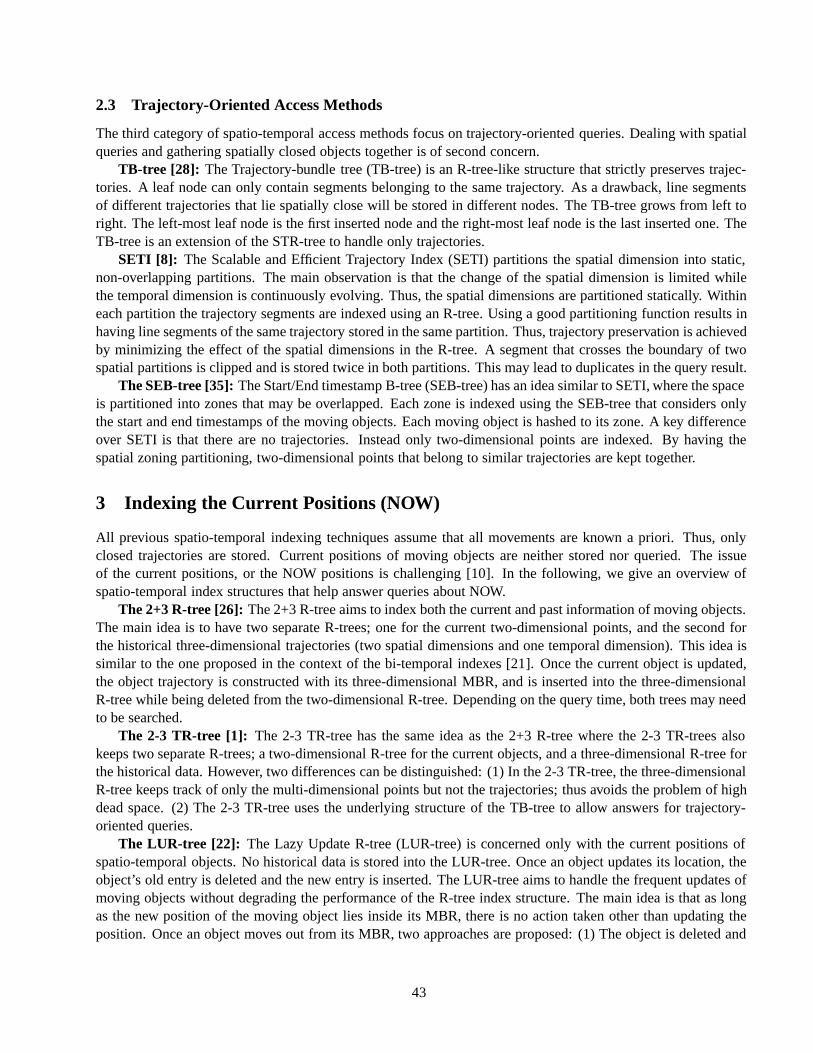
2.3 Trajectory-Oriented Access Methods

The third category of spatio-temporal access methods focus on trajectory-oriented queries. Dealing with spatialqueries and gathering spatially closed objects together is of second concern.

TB-tree [28]: The Trajectory-bundle tree (TB-tree) is an R-tree-like structure that strictly preserves trajec-tories. A leaf node can only contain segments belonging to the same trajectory. As a drawback, line segmentsof different trajectories that lie spatially close will be stored in different nodes. The TB-tree grows from left toright. The left-most leaf node is the first inserted node and the right-most leaf node is the last inserted one. TheTB-tree is an extension of the STR-tree to handle only trajectories.

SETI [8]: The Scalable and Efficient Trajectory Index (SETI) partitions the spatial dimension into static,non-overlapping partitions. The main observation is that the change of the spatial dimension is limited whilethe temporal dimension is continuously evolving. Thus, the spatial dimensions are partitioned statically. Withineach partition the trajectory segments are indexed using an R-tree. Using a good partitioning function results inhaving line segments of the same trajectory stored in the same partition. Thus, trajectory preservation is achievedby minimizing the effect of the spatial dimensions in the R-tree. A segment that crosses the boundary of twospatial partitions is clipped and is stored twice in both partitions. This may lead to duplicates in the query result.

The SEB-tree [35]:The Start/End timestamp B-tree (SEB-tree) has an idea similar to SETI, where the spaceis partitioned into zones that may be overlapped. Each zone is indexed using the SEB-tree that considers onlythe start and end timestamps of the moving objects. Each moving object is hashed to its zone. A key differenceover SETI is that there are no trajectories. Instead only two-dimensional points are indexed. By having thespatial zoning partitioning, two-dimensional points that belong to similar trajectories are kept together.

3 Indexing the Current Positions (NOW)

All previous spatio-temporal indexing techniques assume that all movements are known a priori. Thus, onlyclosed trajectories are stored. Current positions of moving objects are neither stored nor queried. The issueof the current positions, or the NOW positions is challenging [10]. In the following, we give an overview ofspatio-temporal index structures that help answer queries about NOW.

The 2+3 R-tree [26]:The 2+3 R-tree aims to index both the current and past information of moving objects.The main idea is to have two separate R-trees; one for the current two-dimensional points, and the second forthe historical three-dimensional trajectories (two spatial dimensions and one temporal dimension). This idea issimilar to the one proposed in the context of the bi-temporal indexes [21]. Once the current object is updated,the object trajectory is constructed with its three-dimensional MBR, and is inserted into the three-dimensionalR-tree while being deleted from the two-dimensional R-tree. Depending on the query time, both trees may needto be searched.

The 2-3 TR-tree [1]: The 2-3 TR-tree has the same idea as the 2+3 R-tree where the 2-3 TR-trees alsokeeps two separate R-trees; a two-dimensional R-tree for the current objects, and a three-dimensional R-tree forthe historical data. However, two differences can be distinguished: (1) In the 2-3 TR-tree, the three-dimensionalR-tree keeps track of only the multi-dimensional points but not the trajectories; thus avoids the problem of highdead space. (2) The 2-3 TR-tree uses the underlying structure of the TB-tree to allow answers for trajectory-oriented queries.

The LUR-tree [22]: The Lazy Update R-tree (LUR-tree) is concerned only with the current positions ofspatio-temporal objects. No historical data is stored into the LUR-tree. Once an object updates its location, theobject’s old entry is deleted and the new entry is inserted. The LUR-tree aims to handle the frequent updates ofmoving objects without degrading the performance of the R-tree index structure. The main idea is that as longas the new position of the moving object lies inside its MBR, there is no action taken other than updating theposition. Once an object moves out from its MBR, two approaches are proposed: (1) The object is deleted and

43

is reinserted causing the necessary merge and split operations. (2) If the object does not move very far from theMBR, the MBR can be extended to enclose the new location.

Bottom-up Updates [23]: The bottom-up approach for updating R-trees extends the idea of the LUR-tree.Several bottom-up approaches are investigated to accommodate the frequent updates of the moving objects.Examples of these approaches are extending the MBR to enclose the new value and moving the current object toone of the siblings. To avoid excessive I/O’s while investigating the siblings and parents for updates, a compactmain memory summary structure is introduced.

Hashing [34]: Another approach for keeping only the current information is proposed via hashing. Thespace is partitioned into zones that may be overlapped. An object does not update its entry to the databaseuntil it changes its zone. Thus the database always contains an approximated view of the moving object. Toresolve this uncertainty, a filter layer is introduced between the database and the moving objects. The filter layercontains the exact positions of the moving objects. A range query is transformed into a set of zones. If one zoneis completely enclosed in the range query, then all the zones entries are returned in the query result. However, ifa zone intersects with the range queries, then the zone entries need to be sent to the filter layer to check whetherthey satisfy the range query or not.

4 Indexing the Current and Future Positions (NOW and the Future)

In this section, we are concerned about the current and future positions of moving objects. To predict the futurepositions of moving objects, we need to store extra information (e.g., the velocity and the destination). The mo-tion of a moving object in theD-dimensional space is modeled by a reference location�xref = (x1, x2, · · · , xd)at a reference timetref and a velocity vector�v = (v1, v2, · · · , vd). The predicted location�xt of the movingobject at any instance timet > tref can be computed by�xt = �xref + �v(t − tref ). For simplicity, we willassume that objects move in the one-dimensional space. The object movement is modeled by the linear equationxt = at + b, wherea andb are constants. Notice thata indicates the constant velocity of the moving object andb is the starting location of the moving object. Also, we assume that the reference location is computed at timetref = 0.

4.1 The Original Space-Time Space

By plotting the equationxt = at + b in the two-dimensional space, where the horizontal space represents thetime and the vertical space represents the location, we obtain a set of line segments in the time-space domain.Then, the problem of indexing future positions is transformed to indexing a set of two-dimensional lines wherespatial access methods can be used [11].

PMR-quadtree for moving objects [40]: Tayeb et al. [40] use the PMR-quadtree [27] as their underlyingspatial access methods for indexing the future trajectories. A key point is that when an update of moving objectsoccur, the whole index structure is destroyed and is rebuilt given the new information. To avoid excessiveupdate operations, the index is rebuilt every∆T time units. In the abstract level, the infinite time dimension ispartitioned into equal size time slices, each with size∆T . For each slice, a new PMR-quadtree is built based onthe motion equation. However, due to the storage limit, only the current PMR-Quadtree is stored.

Generally, using spatial access methods to index the future trajectories has two main drawbacks: (1) Largeamount of dead space due to representing the trajectory by its minimum bounding rectangle. (2) Data is skewedsince all the trajectories have the same end time value.

4.2 Transformation Methods

To overcome the drawbacks of spatio-temporal indexing in the time-space domain, the time-space domain istransformed into another space. The main idea is that it is easier to represent and query the data in this new

44

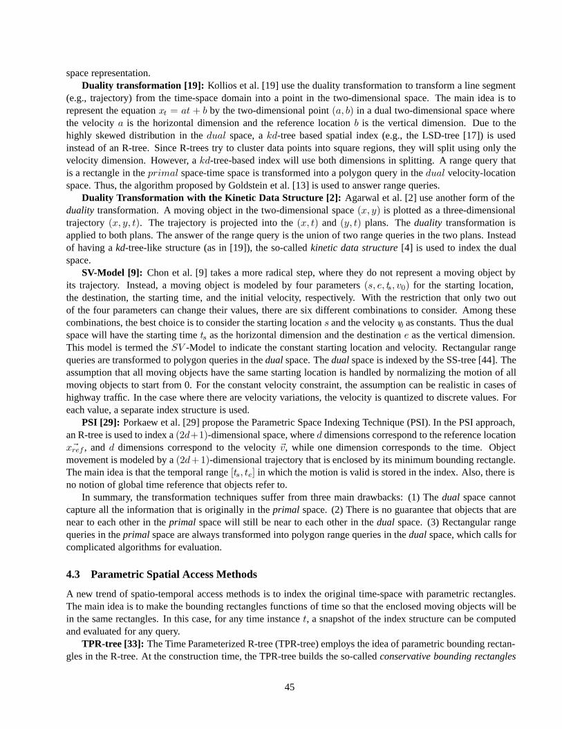
space representation.Duality transformation [19]: Kollios et al. [19] use the duality transformation to transform a line segment

(e.g., trajectory) from the time-space domain into a point in the two-dimensional space. The main idea is torepresent the equationxt = at + b by the two-dimensional point(a, b) in a dual two-dimensional space wherethe velocitya is the horizontal dimension and the reference locationb is the vertical dimension. Due to thehighly skewed distribution in thedual space, akd-tree based spatial index (e.g., the LSD-tree [17]) is usedinstead of an R-tree. Since R-trees try to cluster data points into square regions, they will split using only thevelocity dimension. However, akd-tree-based index will use both dimensions in splitting. A range query thatis a rectangle in theprimal space-time space is transformed into a polygon query in thedual velocity-locationspace. Thus, the algorithm proposed by Goldstein et al. [13] is used to answer range queries.

Duality Transformation with the Kinetic Data Structure [2]: Agarwal et al. [2] use another form of theduality transformation. A moving object in the two-dimensional space(x, y) is plotted as a three-dimensionaltrajectory(x, y, t). The trajectory is projected into the(x, t) and (y, t) plans. Theduality transformation isapplied to both plans. The answer of the range query is the union of two range queries in the two plans. Insteadof having akd-tree-like structure (as in [19]), the so-calledkinetic data structure[4] is used to index the dualspace.

SV-Model [9]: Chon et al. [9] takes a more radical step, where they do not represent a moving object byits trajectory. Instead, a moving object is modeled by four parameters(s, e, ts, v0) for the starting location,the destination, the starting time, and the initial velocity, respectively. With the restriction that only two outof the four parameters can change their values, there are six different combinations to consider. Among thesecombinations, the best choice is to consider the starting locations and the velocityv0 as constants. Thus the dualspace will have the starting timets as the horizontal dimension and the destinatione as the vertical dimension.This model is termed theSV -Model to indicate the constant starting location and velocity. Rectangular rangequeries are transformed to polygon queries in thedualspace. Thedualspace is indexed by the SS-tree [44]. Theassumption that all moving objects have the same starting location is handled by normalizing the motion of allmoving objects to start from 0. For the constant velocity constraint, the assumption can be realistic in cases ofhighway traffic. In the case where there are velocity variations, the velocity is quantized to discrete values. Foreach value, a separate index structure is used.

PSI [29]: Porkaew et al. [29] propose the Parametric Space Indexing Technique (PSI). In the PSI approach,an R-tree is used to index a(2d+1)-dimensional space, whered dimensions correspond to the reference location�xref , andd dimensions correspond to the velocity�v, while one dimension corresponds to the time. Object

movement is modeled by a(2d+1)-dimensional trajectory that is enclosed by its minimum bounding rectangle.The main idea is that the temporal range[ts, te] in which the motion is valid is stored in the index. Also, there isno notion of global time reference that objects refer to.

In summary, the transformation techniques suffer from three main drawbacks: (1) Thedual space cannotcapture all the information that is originally in theprimal space. (2) There is no guarantee that objects that arenear to each other in theprimal space will still be near to each other in thedual space. (3) Rectangular rangequeries in theprimal space are always transformed into polygon range queries in thedual space, which calls forcomplicated algorithms for evaluation.

4.3 Parametric Spatial Access Methods

A new trend of spatio-temporal access methods is to index the original time-space with parametric rectangles.The main idea is to make the bounding rectangles functions of time so that the enclosed moving objects will bein the same rectangles. In this case, for any time instancet, a snapshot of the index structure can be computedand evaluated for any query.

TPR-tree [33]: The Time Parameterized R-tree (TPR-tree) employs the idea of parametric bounding rectan-gles in the R-tree. At the construction time, the TPR-tree builds the so-calledconservative bounding rectangles

45

that enclose a set of moving objects. The lower bound of the conservative bounding rectangle is set to move withthe minimum speed of the enclosed points, while the upper bound is set to move with the maximum speed ofthe enclosed points. In this case, the conservative bounding rectangle never shrinks, and is guaranteed to alwayscontain the enclosed moving objects. To avoid the case where the bounding rectangles grow to be very large,whenever the position of an objecto is updated, all the bounding rectangles on the nodes along the path to theleaf at whicho is stored are recomputed.

PR-tree [7]: The PR-tree is similar to the TPR-tree. However, the PR-tree considers the problem of movingobjects with spatial extents that are represented by parametric rectangles. Each parametric rectangle has a timeinterval that represents the start time and the end time of its movement. In contrast to the TPR-tree, whereobjects are considered moving forever, the PR-tree has the knowledge of the end time of moving objects. Thus amoving object is represented as a polygon on the space rather than a trajectory. Given the movement end times,the bounding rectangles of a set of moving objects (represented as polygons) can be computed as the convexhull of the moving objects.

NSI [29]: The NSI tree is similar to the TPR-tree in the sense that both define parametric bounding rectanglesfor moving objects. However, the difference is in the way the bounding rectangle is defined.

VCI R-tree [30]: The main idea of the Velocity Constrained Indexing (VCI) is to add an additional fieldvmax to each R-tree node.vmax stores the maximum allowed speed over all objects covered by this node. Forany query at timet, all bounding rectangles are expanded usingvmax. This approach is similar to that of theTPR-tree in the sense that both trees consider expanding the bounding rectangles over time to contain all theenclosed objects. However, the underlying model is different. In VCI indexing, there is no need to know theexact speed of each moving object. Instead, there is a restriction that all moving objects cannot exceed a certainmaximum speed. In the TPR-tree, the exact velocity of moving objects is needed. On the other side, many falsepositives appear in the VCI indexing. The VCI indexing is designed specially to handle the issue of the sharedexecution of continuous queries.

STAR-tree [31]: The Spatio-temporal Self Adjusting R-tree (STAR-tree) is similar to the TPR-tree, with theintroduction of the notion ofself-adjustment. Whenever the query performance degrades, the STAR-tree adjustsitself without any input from the user.

REXP -tree [32]: TheREXP -tree is an extension of the TPR-tree to handle moving objects with expirationtimes. The main idea is to avoid the drawback that may result for moving objects that do not update theirmovement for a long time. To benefit from the expiration time information, theREXP -tree employs a new typeof bounding regions. In addition, theREXP -tree implements a lazy technique for removing expired entries fromthe index until the bounding rectangles are recomputed.

TPR*-tree [39]: The TPR*-tree uses exactly the same structure and assumptions as the TPR-tree [33].Unlike the TPR-tree where it uses the same insert and delete functions of the R*-tree, the TPR*-tree provides anew set of insertion and deletion algorithms that aim at minimizing a certain cost function.

5 Available Indexing Toolkits

In this section, we give a brief overview of publicly available indexing toolkits that can be used to implementspatio-temporal access methods.

5.1 GiST: Generalized Search Trees for Database Systems

GiST [16] defines a framework of basic interfaces required to construct a hierarchical access method for databasesystems. GiST supports the class of balanced trees (e.g., the B-tree, the R-tree, and the SR-tree [18]). The mainarchitecture of GiST contains two parts:internal methods andtype-specificmethods. Internal methods are thecommon methods to all balanced trees (e.g., search, insert, and delete). Such methods are hard-coded inside

46

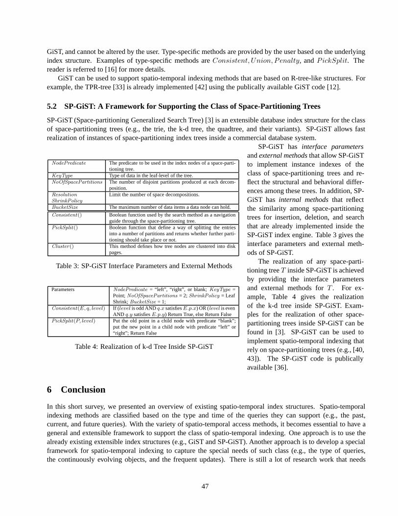
GiST, and cannot be altered by the user. Type-specific methods are provided by the user based on the underlyingindex structure. Examples of type-specific methods areConsistent, Union, Penalty, andPickSplit. Thereader is referred to [16] for more details.

GiST can be used to support spatio-temporal indexing methods that are based on R-tree-like structures. Forexample, the TPR-tree [33] is already implemented [42] using the publically available GiST code [12].

5.2 SP-GiST: A Framework for Supporting the Class of Space-Partitioning Trees

SP-GiST (Space-partitioning Generalized Search Tree) [3] is an extensible database index structure for the classof space-partitioning trees (e.g., the trie, the k-d tree, the quadtree, and their variants). SP-GiST allows fastrealization of instances of space-partitioning index trees inside a commercial database system.

NodePredicate The predicate to be used in the index nodes of a space-parti-tioning tree.

KeyType Type of data in the leaf-level of the tree.NoOfSpacePartitions The number of disjoint partitions produced at each decom-

position.ResolutionShrinkPolicy

Limit the number of space decompositions.

BucketSize The maximum number of data items a data node can hold.

Consistent() Boolean function used by the search method as a navigationguide through the space-partitioning tree.

PickSplit() Boolean function that define a way of splitting the entriesinto a number of partitions and returns whether further parti-tioning should take place or not.

Cluster() This method defines how tree nodes are clustered into diskpages.

Table 3: SP-GiST Interface Parameters and External Methods

SP-GiST hasinterface parametersandexternal methodsthat allow SP-GiSTto implement instance indexes of theclass of space-partitioning trees and re-flect the structural and behavioral differ-ences among these trees. In addition, SP-GiST has internal methodsthat reflectthe similarity among space-partitioningtrees for insertion, deletion, and searchthat are already implemented inside theSP-GiST index engine. Table 3 gives theinterface parameters and external meth-ods of SP-GiST.

Parameters NodePredicate = “left”, “right”, or blank; KeyType =Point;NoOfSpacePartitions = 2; ShrinkPolicy = LeafShrink;BucketSize = 1;

Consistent(E, q, level) If ( level is odd ANDq.x satisfiesE.p.x) OR (level is evenAND q.y satisfiesE.p.y) Return True, else Return False

PickSplit(P, level) Put the old point in a child node with predicate “blank”;put the new point in a child node with predicate “left” or“right”; Return False

Table 4: Realization of k-d Tree Inside SP-GiST

The realization of any space-parti-tioning treeT inside SP-GiST is achievedby providing the interface parametersand external methods forT . For ex-ample, Table 4 gives the realizationof the k-d tree inside SP-GiST. Exam-ples for the realization of other space-partitioning trees inside SP-GiST can befound in [3]. SP-GiST can be used toimplement spatio-temporal indexing thatrely on space-partitioning trees (e.g., [40,43]). The SP-GiST code is publicallyavailable [36].

6 Conclusion

In this short survey, we presented an overview of existing spatio-temporal index structures. Spatio-temporalindexing methods are classified based on the type and time of the queries they can support (e.g., the past,current, and future queries). With the variety of spatio-temporal access methods, it becomes essential to have ageneral and extensible framework to support the class of spatio-temporal indexing. One approach is to use thealready existing extensible index structures (e.g., GiST and SP-GiST). Another approach is to develop a specialframework for spatio-temporal indexing to capture the special needs of such class (e.g., the type of queries,the continuously evolving objects, and the frequent updates). There is still a lot of research work that needs

47

to be investigated in spatio-temporal indexing. Most of the work so far supports selection operators and rangequeries. More research is needed to support other kinds of operators (e.g., spatio-temporal join) and queries(e.g., nearest-neighbor queries).

References

[1] M. Abdelguerfi, J. Givaudan, K. Shaw, and R. Ladner. The 2-3 TR-tree, A Trajectory-Oriented Index Structure forFully Evolving Valid-time Spatio-temporal Datasets. InProc. of the ACM workshop on Adv. in Geographic Info.Sys., ACM GIS, pages 29–34, Nov. 2002.

[2] P. K. Agarwal, L. Arge, and J. Erickson. Indexing Moving Points. InProc. of the ACM Symp. on Principles ofDatabase Systems, PODS, pages 175–186, May 2000.

[3] W. G. Aref and I. F. Ilyas. SP-GiST: An Extensible Database Index for Supporting Space Partitioning Trees.Journalof Intelligent Information Systems , JIIS, 17(2-3):215–240, 2001.

[4] J. Basch, L. J. Guibas, and J. Hershberger. Data structures for mobile data. InProc. of the ACM-SIAM symposiumon Discrete algorithms, SODA, pages 747–756, 1997.

[5] B. Becker, S. Gschwind, T. Ohler, B. Seeger, and P. Widmayer. An Asymptotically Optimal Multiversion B-Tree.VLDB Journal, 5(4):264–275, 1996.

[6] F. W. Burton, J. G. Kollias, D. G. Matsakis, and V. G. Kollias. Implementation of Overlapping B-trees for Time andSpace Efficient Representation of Collections of Similar Files.The Computer Journal, 33(3):279–280, 1990.

[7] M. Cai and P. Revesz. Parametric R-Tree: An Index Structure for Moving Objects. InProc. of the Intl. Conf. onManagement of Data, COMAD, Dec. 2000.

[8] V. P. Chakka, A. Everspaugh, and J. M. Patel. Indexing Large Trajectory Data Sets with SETI. InProc. of the Conf.on Innovative Data Systems Research, CIDR, Asilomar, CA, Jan. 2003.

[9] H. D. Chon, D. Agrawal, and A. E. Abbadi. Storage and Retrieval of Moving Objects. InMobile Data Management,pages 173–184, Jan. 2001.

[10] J. Clifford, C. E. Dyreson, T. Isakowitz, C. S. Jensen, and R. T. Snodgrass. On the Semantics of “Now” in Databases.ACM Trans. on Database Systems , TODS, 22(2), 1997.

[11] V. Gaede and O. Günther. Multidimensional Access Methods.ACM Computing Surveys, 30(2):170–231, 1998.

[12] GiST: http://gist.cs.berkeley.edu/.

[13] J. Goldstein, R. Ramakrishnan, U. Shaft, and J.-B. Yu. Processing Queries By Linear Constraints. InProc. of theACM Symp. on Principles of Database Systems, PODS, pages 257–267, May 1997.

[14] A. Guttman. R-Trees: A Dynamic Index Structure for Spatial Searching. InProc. of the ACM Intl. Conf. onManagement of Data, SIGMOD, pages 47–57, June 1984.

[15] M. Hadjieleftheriou, G. Kollios, V. J. Tsotras, and D. Gunopulos. Efficient Indexing of Spatiotemporal Objects. InProc. of the Intl. Conf. on Extending Database Technology, EDBT, pages 251–268, Czech Republic, Mar. 2002.

[16] J. M. Hellerstein, J. F. Naughton, and A. Pfeffer. Generalized Search Trees for Database Systems. InProc. of theIntl. Conf. on Very Large Data Bases, VLDB, pages 562–573, Sept. 1995.

[17] A. Henrich, H.-W. Six, and P. Widmayer. The lsd tree: Spatial access to multidimensional point and nonpoint objects.In Proc. of the Intl. Conf. on Very Large Data Bases, VLDB, pages 45–53, Aug. 1989.

[18] N. Katayama and S. Satoh. The SR-tree: An Index Structure for High-Dimensional Nearest Neighbor Queries. InProc. of the ACM Intl. Conf. on Management of Data, SIGMOD, pages 369–380, May 1997.

[19] G. Kollios, D. Gunopulos, and V. J. Tsotras. On Indexing Mobile Objects. InProc. of the ACM Symp. on Principlesof Database Systems, PODS, pages 261–272, June 1999.

[20] G. Kollios, V. J. Tsotras, D. Gunopulos, A. Delis, and M. Hadjieleftheriou. Indexing Animated Objects UsingSpatiotemporal Access Methods.IEEE Trans. on Knowledge and Data Engineering, TKDE, 13(5):758–777, 2001.

[21] A. Kumar, V. J. Tsotras, and C. Faloutsos. Designing Access Methods for Bitemporal Databases.IEEE Trans. onKnowledge and Data Engineering, TKDE, 10(1):1–20, 1998.

48

[22] D. Kwon, S. Lee, and S. Lee. Indexing the Current Positions of Moving Objects Using the Lazy Update R-tree. InMobile Data Management, MDM, pages 113–120, Jan. 2002.

[23] M. Lee, W. Hsu, C. Jensen, B. Cui, and K. Teo. Supporting Frequent Updates in R-Trees: A Bottom-Up Approach.In Proc. of the Intl. Conf. on Very Large Data Bases, VLDB, Sept. 2003.

[24] D. B. Lomet and B. Salzberg. Access Methods for Multiversion Data. InProc. of the ACM Intl. Conf. on Managementof Data, SIGMOD, pages 315–324, May 1989.

[25] M. A. Nascimento and J. R. O. Silva. Towards historical R-trees. InProc. of the ACM Symp. on Applied Computing,SAC, pages 235–240, Feb. 1998.

[26] M. A. Nascimento, J. R. O. Silva, and Y. Theodoridis. Evaluation of Access Structures for Discretely Moving Points.In Proc. of the Intl. Workshop on Spatio-Temporal Database Management, STDBM, pages 171–188, Sept. 1999.

[27] R. C. Nelson and H. Samet. A Consistent Hierarchical Representation for Vector Data. InProc. of the ACM SIG-GRAPH, pages 197–206, Aug. 1986.

[28] D. Pfoser, C. S. Jensen, and Y. Theodoridis. Novel Approaches in Query Processing for Moving Object Trajectories.In Proc. of the Intl. Conf. on Very Large Data Bases, VLDB, pages 395–406, Sept. 2000.

[29] K. Porkaew, I. Lazaridis, and S. Mehrotra. Querying Mobile Objects in Spatio-Temporal Databases. InProc. of theIntl. Symp. on Advances in Spatial and Temporal Databases, SSTD, pages 59–78, Redondo Beach, CA, July 2001.

[30] S. Prabhakar, Y. Xia, D. V. Kalashnikov, W. G. Aref, and S. E. Hambrusch. Query Indexing and Velocity ConstrainedIndexing: Scalable Techniques for Continuous Queries on Moving Objects.IEEE Transactions on Computers,51(10):1124–1140, 2002.

[31] C. M. Procopiuc, P. K. Agarwal, and S. Har-Peled. STAR-Tree: An Efficient Self-Adjusting Index for MovingObjects. InProc. of the Workshop on Alg. Eng. and Experimentation, ALENEX, pages 178–193, Jan. 2002.

[32] S. Saltenis and C. S. Jensen. Indexing of Moving Objects for Location-Based Services. InProc. of the Intl. Conf. onData Engineering, ICDE, Feb. 2002.

[33] S. Saltenis, C. S. Jensen, S. T. Leutenegger, and M. A. Lopez. Indexing the Positions of Continuously MovingObjects. InProc. of the ACM Intl. Conf. on Management of Data, SIGMOD, pages 331–342, May 2000.

[34] Z. Song and N. Roussopoulos. Hashing Moving Objects. InMobile Data Management, pages 161–172, Jan. 2001.

[35] Z. Song and N. Roussopoulos. SEB-tree: An Approach to Index Continuously Moving Objects. InMobile DataManagement, MDM, pages 340–344, Jan. 2003.

[36] SP-GiST: http://www.cs.purdue.edu/homes/aref/dbsystemsfiles/SP-GiST/index.html.

[37] Y. Tao and D. Papadias. Efficient Historical R-trees. InProc. of the Intl. Conf. on Scientific and Statistical DatabaseManagement, SSDBM, pages 223–232, July 2001.

[38] Y. Tao and D. Papadias. MV3R-Tree: A Spatio-Temporal Access Method for Timestamp and Interval Queries. InProc. of the Intl. Conf. on Very Large Data Bases, VLDB, pages 431–440, Sept. 2001.

[39] Y. Tao, D. Papadias, and J. Sun. The TPR*-Tree: An Optimized Spatio-temporal Access Method for PredictiveQueries. InProc. of the Intl. Conf. on Very Large Data Bases, VLDB, Sept. 2003.

[40] J. Tayeb,O. Ulusoy, and O. Wolfson. A Quadtree-Based Dynamic Attribute Indexing Method.The ComputerJournal, 41(3):185–200, 1998.

[41] Y. Theodoridis, M. Vazirgiannis, and T. Sellis. Spatio-Temporal Indexing for Large Multimedia Applications. InProc. of the IEEE Conference on Multimedia Computing and Systems, ICMCS, June 1996.

[42] TPR-tree: http://www.cs.auc.dk/TimeCenter/software.htm.

[43] T. Tzouramanis, M. Vassilakopoulos, and Y. Manolopoulos. Overlapping Linear Quadtrees: A Spatio-TemporalAccess Method. InProc. of the ACM workshop on Adv. in Geographic Info. Sys., ACM GIS, pages 1–7, Nov. 1998.

[44] D. A. White and R. Jain. Similarity Indexing with the SS-tree. InProc. of the Intl. Conf. on Data Engineering, ICDE,pages 516–523, Feb. 1996.

[45] X. Xu, J. Han, and W. Lu. RT-Tree: An Improved R-Tree Indexing Structure for Temporal Spatial Databases. InProc. of the Intl. Symp. on Spatial Data Handling, SDH, pages 1040–1049, July 1990.

49

Spatio-Temporal Data Exchange Standards

Albrecht Schmidt Christian S. Jensen

Department of Computer Science, Aalborg University, Denmark{al,csj}@cs.auc.dk

Abstract

We believe that research that concerns aspects of spatio-temporal data management may benefit fromtaking into account the various standards for spatio-temporal data formats. For example, this may con-tribute to rendering prototype software “open” and more readily useful. This paper thus identifies andbriefly surveys standardization in relation to primarily the exchange and integration of spatio-temporaldata. An overview of several data exchange languages is offered, along with reviews their potential forfacilitating the collection of test data and the leveraging of prototypes. The standards, most of which areXML-based, lend themselves to the integration of prototypes into middleware architectures, e.g., as Webservices.

1 Introduction

It is often important to be able to test new spatial and temporal query processing techniques with real-worlddata. This contributes to understanding how the techniques will perform in specific production settings. Overthe years, a number of data sets have become publicly available that, along with synthetic data, can serve as abasis for experimenting with software prototypes. However, since many of these data sets are only available incustom formats, a fair amount of domain knowledge is required to make use of them. Recent standardizationefforts, which typically employ XML-based technologies and digital library data exchange formats, aim tofacilitate the communication between applications by specifying data exchange standards. Especially, XML-based geo-enabled applications can be deployed and enriched with the plethora of query languages, constraintdefinition languages, and extensibility opportunities that are part of the standards infrastructure.

This paper surveys spatio-temporal data exchange standardization efforts. They all have different historiesand stem from different sub-communities. They thus come with both advantages and disadvantages in the eyesof a potential user. The standards not only deliver exact specifications of data structures, but also address meta-data issues. For example, it is often useful to know the validity, accuracy, and reliability of a measurement or itsorigin. In this sense, data exchange standards do not only serve as an exchange mechanism for data structures,but are also helpful in more advance applications like, e.g., decision support systems.

In particular, we survey the Geography Markup Language [12], which is the foremost candidate for address-ing the manifold needs of the geographical community. We also survey the Scalable Vector Graphics (SVG)standard [8]. SVG is an XML-based language for the description and presentation oftwo-dimensionalvector


50

and raster data. Next, we cover the ISO Technical Committee 211, which is central to the standardization of geo-graphic data [1]. The US Federal Geographic Data Committee [3], another active player, is also covered briefly.At least a handful of other (XML-based) standards exist that do not seem to be driven by large communities, butare still of interest. For reference and completeness, these are covered briefly.

Generally, we observe a trend towards XML-based standards. A recent book [11] provides a very readableintroduction to data exchange in geographical applications. Many of the XML languages covered in this paperadhere to the fundamental principle of separating content from presentation: data are encoded according tosemantic criteria without constraining how the data may be presented to a human or consumed by an application.

Sections 2 and 3 cover GML and SVG, respectively. Then the ISO Technical Committee 211 and the FederalGeographic Data Committee are covered in Sections 4 and 5, respectively. Section 6 presents the “minor”standards, and Section 7 summarizes the paper.

2 Geography Markup Language (GML)

The Geography Markup Language (GML) [12] is an XML language created under the auspices of the Open GISConsortium, whose mission statement is to facilitate the “full integration of geospatial data and geoprocessingresources into mainstream computing and to foster the widespread use of inter operable geoprocessing softwareand geodata products throughout the information infrastructure” [4]. GML, which could be considered the flag-ship effort in geoprocesssing, is a multi-stage effort that has reached version 3.0. By designing the language inmultiple stages, the standardization body wants to make sure that the language evolves naturally and incorpo-rates more and more features over time. For example, the so-calledsimplefeatures have been defined and beenintegrated in the releases leading up to version 2.0.

GML’s definition is based on XML Schema and tries to take advantage of its full feature set. For example, itmakes it possible for users to tailor the language to their needs by means of XML schema’s extensibility. So itis possible to incorporate well-defined GML schema fragments into documents that follow a user’s applicationschema.

Therefore GML is able to describe a wide variety of geographical objects by combining its built-in datatypes, which implement the OGC Simple Features model [4], with the extensibility features of XML. Being anapplication of XML, GML is designed to take advantage of the XML standards framework; documents can bereadily transformed into a variety of presentation formats, most notably vector formats and raster graphics suchas maps.

Future versions of GML are planned to include additional aspects. Version 3.0 has added features for tempo-ral GIS, including time stamps, events, and histories, as well as units of measure and the possibility of groupingfeatures into layers, to name but a few. But since GML is used in practice and competing standards convergewith it, many users consider it mature at its current stage and take advantage of its features.

For researchers, the advantages of using GML include the availability of test data sets and the incentive touse the modeling knowledge of the geographic data management community in their prototypes, which can inturn be more flexibly leveraged by other researchers and industrial partners alike. Due to the strict semantics ofGML, there is also the potential to benefit from the domain modeling that is part of the standard.

3 Scalable Vector Graphics (SVG)

SVG (Scalable Vector Graphics) is a standard developed under the auspices of the World Wide Web Consortium(W3C) [5]. It defines features and syntax for describingtwo-dimensionalvector and raster graphics in XML. Itis thus primarily oriented towards presentation.

SVG knows three kinds of graphical objects: composite vector elements, e.g., paths that consist of lines andcurves, as well as images and text. The graphical objects can be grouped, styled, transformed, and composited

51

with various operations like nested transformations, clipping paths, alpha masks, filter effects, templates aswell as previously rendered objects. Furthermore, SVG objects can be interactive and dynamic. This is achievedthrough event-handlers and a well-defined interface: Care has been taken to ensure interoperability with scriptinglanguages. To this end, SVG features event handlers for user interaction, e.g., using a mouse-related events like“onmouseover”, and the SVG Document Object Model for well-defined transformations and manipulations bymeans of scripting languages. Additionally, animations can be defined and triggered either declaratively, i.e., byembedding SVG animation elements into SVG content or by using the aforementioned scripting interface.

SVG comprises a comprehensive list of built-in graphical elements: path, text, rect, circle, ellipse, line,polyline, polygon, image, and use – a mechanism to reference SVG elements. A particularly important aspect ofSVG drawings isreusability. Through symbol mechanisms, users may build libraries of graphical elements andre-use them without having to register at a centralized directory. To blend with the other elements of applica-tions at client-side rendering of presentations, SVG also allows declarative definitions of filters for rasterization.Additionally, SVG provides sophisticated handling of fonts so that the original text is preserved with respectto indexing, search, and the graphical appearance intended by the authors. SVG content may be included via astand-alone document, inline embedding, references like links, or style sheets.

The benefits researchers get from using SVG in their projects range from software engineering considera-tions to data re-use and integration opportunities. For example, the time it takes to prototype visual applicationscan be significantly reduced by using an SVG viewer instead of a custom-built user interface. Viewers are avail-able for many different types of devices, including mobile phones, personal digital assistants, and navigatorsembeddable in conventional graphical user interfaces. Additionally, the tight integration and interoperabilityof the XML standards facilitates the development of robust applications by providing a language glue that isexpressive enough to capture the semantics of the different domain models. For instance, SVG applications candirectly benefit from the availability of meta-information encoded in GML documents. Furthermore, the abilityof SVG to combine different source data, such as raster graphics, vector graphics, and fonts, in a single datamodels provides application programmers with a uniform interface and greatly reduces the need to learn andunderstand more than one API.

4 ISO/TC 211

ISO is the primary international standards organization for information technology. The ISO Technical Com-mittee 211, on Geographic information/Geomatics, has as its objective to create standards for “[...] informa-tion concerning objects or phenomena that are directly or indirectly associated with a location relative to theEarth” [1]. Because the ISO/TC 211 adopts a service-oriented view of geoprocessing, its standards concern awide variety of uses of geographic data, including methods, tools, and services that relate to data management,acquiring, processing, analyzing, accessing, presenting, and exchanging data. As a result, the ISO 19100 seriesstandards produced by the ISO/TC 211 go well beyond plain data modeling. Further, GML, which is known asISO 19136 in this context, is only one component of this larger series of standards developed under the auspicesof the ISO/TC 211.

The interoperability of standards is of particular interest to the ISO/TC 211. For example, the committeehas to ensure that the standards for position services (ISO 19116), location-based services (ISO 19132/3), andmultimodal services (ISO 19134) integrate smoothly with GML.

The overall aim is to increase the availability, access, integration, and sharing of geographic information, andto enable interoperability of geospatially enabled computer systems [1] as well as to contribute to the creation ofa community that supports the dissemination of geographic understanding and enables sustained development.

The focus of the ISO/TC 211 on providing an overarching standardization framework has several notableadvantages. The adoption of such a framework is expected to result in lower training costs, better comparabilityof results, increased planning safety by relying on a mature foundation as well as the existence of a knowledge-

52

able and experienced community for consulting and collaboration. So planning and implementation will be lesserror-prone, and interoperability is achieved more easily. In this sense, the standardized framework is the answerto many practical questions.

Also, the ISO/TC 211 can be seen as an umbrella intended to cover all areas native to geoprocessing. Con-sequently, basic familiarity with this effort provides an interesting overview of a multi-faceted research area.

5 Federal Geographic Data Committee (FGDC)

The Federal Geographic Data Committee [3] is a US governmental, inter-agency committee. The FGDC iscentral to the effort that develops the US National Spatial Data Infrastructure. New standards are developedby the FGDC only when there are no existing standards that are suitable for governmental use. A number ofgeographic data and metadata standards have been developed and are available online (see [3]).

As part of its objectives, the FGDC aims to enable the simultaneously reduction of data production costs andimprovement of data quality by providing a foundation for sharing geographic data among government agencies.A complementary goal was to increase data availability, not only to the public sector, but also to academia andthe private sector.

6 Standards for Specific Application Domains

We proceed to cover some efforts that are not part of the “big” standards. All of these standards are XML based.The three first are early examples of XML being deployed in the transportation industry. In addition to offeringdata models, these standards show how domain specialists model different application domains.

POIX (Point Of Interest eXchange Language) POIX [9] is an XML representation for places and routes. Itwas proposed by a Japanese consortium interested in motor vehicles, traffic, and road networks; car navigationsystems is the application area of primary interest. The purpose of POIX is to provide markup for both thelocations of an object and location-related information. Examples of location-related information include, e.g.,opening hours and other descriptions for shopping locations. POIX also provides facilities for handling localizedinformation such as geodetic or angle units, which may vary from country to country.

NVML (NaVigation Markup Language) NVML (NaVigation Markup Language) [13] is a markup languagefor describing navigation information in vehicle information systems. The main objective of NVML is thedescription of different types of routes. Examples include routes from a current position to a destination, theway to a shop from the nearest train station, transportation courses, sightseeing courses, and tour schedules.Special emphasis is on any-time/anywhere services for a variety of end-user devices.

RWML (Road Web Markup Language) RWML [6] has been being developed at the Civil EngineeringResearch Institute of Hokkaido. This language was developed as part of an effort to support smooth and safedriving under a variety of circumstances. Consequently, RWML includes standard representation syntax forweather and disaster information as well as for messages and announcements from public services.

G-XML The G-XML effort [2] is also Japanese; it has influenced developments in the context of ISO TC/211and tries to maintain harmonization with GML as it itself evolves. The goals of the G-XML effort are similarin spirit to those of many XML applications: creating an encoding of spatial data, thus providing “a method forfreely accessing and using geographic information over the Internet,” according to [2]. GML 3.0 is a G-XMLconverged version, which implies that the underlying data models have been aligned.

53

Sensor Modeling Language (SensorML) SensorML [7] aims to implement an XML data exchange languagefor geolocating data that stems from dynamic sensors. The objective is to cover most or all types of existingsensors, including those installed on satellites, aircrafts, ships, land vehicles, and stationary platforms. It coversmeans for describing sensor-specific information such as location, rotation, timing, target, sensor geometry, dy-namics, and radiometry. It also addresses dependencies among variables. SensorML offers database researchersan overview of a field that so far has been outside the community, and it encourages proper application datamodels. Again, the standard enables data sharing and data exchange as well as increased system modularity andinteroperability.

7 Summary

A rich variety of standards that enable the exchange of geographic data exists. Although standardization hasbeen initiated by committees representing different organizations and communities, in order to serve differentpurposes, the broad acceptance of XML appears to have caused many standards committees to join forces, whichhas resulted in some consolidation of standards. However, because fundamentally different application domainsexist, such as the description of two- or three-dimensional visualizations and the representation of geographic orsensor data, a diversity of standards remains.

We briefly surveyed some of the geoprocessing standards that are of special interest to researchers in spatio-temporal query processing. As part of this, we pointed out in which application domains the standards can bedeployed and what advantages, be it technical, educational, or social, they bring about.

References

[1] ISO TC 211. ISO TC 211 Web Page.http://www.isotc211.org/, 2003.

[2] Database Promotion Center. G-XML – Geospatial-eXtensible Markup Language Version 2.0. available athttp://gisclh01.dpc.or.jp/gxml/contents-e/, 2003.

[3] Federal Geographic Data Committee. Metadata.http://www.fgdc.gov, 2003.

[4] Open GIS Consortium. Homepage.http://www.opengis.org/, 2003.

[5] The World Wide Web Consortium. Homepage.http://www.w3c.org, 2003.

[6] RWML Working Group. Road Web Markup Language (RWML). available athttp://rwml.its-win.gr.jp/eng/index.htm, October 2001.

[7] Open GIS Consortium Inc. Sensor Modeling Language (SensorML). available athttp://stromboli.nsstc.uah.edu/SensorML/, 2002.

[8] J. Ferraiolo (Editor). Scalable Vector Graphics (SVG). available athttp://www.w3.org/TR/SVG/, 2001.

[9] H. Kanemitsu and T. Kamada. POIX: Point Of Interest eXchange Language Specification. available athttp://www.w3.org/TR/poix/, June 1999.

[10] Ron Lake. Geography Markup Language (GML) 2.0 – Enabling the Geo-spatial Web. tutorial available athttp://gislounge.com/ucon/ucgmlintro.shtml, 2003.

[11] Zhong-Ren Peng and Ming-Hsiang Tsou.Internet GIS: Distributed Geographic Information Services for the Internetand Wireless Networks. Wiley, 2003.

[12] S. Cox, A. Cuthbert, R. Lake, and R. Martell. Geography Markup Language (GML) 3.0. available athttp://www.opengis.net/gml/, 2001.

[13] M. Sekiguchi, K. Takayama, H. Naito, Y. Maeda, H. Horai, and M. Toriumi. NaVigation Markup Language (NVML).available athttp://www.w3.org/TR/NVML, August 1999.

References including URLs are current as of May 21, 2003.

54

Sponsored by the

IEEE Computer Society

CALL FOR PAPERS

20th International Conference on Data Engineering March 30 - April 2, 2004

Omni Parker House Hotel, Boston, USA http://www.cse.uconn.edu/cse/icde04

Data Engineering deals with the use of engineering techniques and methodologies in the design, development and assess-ment of information systems for different computing platforms and application environments. The 20th International Confe-rence on Data Engineering will be held in Boston, Massachusetts, USA -- an academic and technological center with a variety of historical and cultural attractions of international prominence within walking distance. _________________________________________________________________________________________

The ICDE 2004 International Conference on Data Engineering provides a premier forum for:

sharing research solutions to problems of today's information society; exposing practicing engineers to evolving research, tools, and prac-tices and providing them with an early opportunity to evaluate these;

raising awareness in the research community of the problems of prac-tical applications of data engineering;

promoting the exchange of data engineering technologies and experi-ence among researchers and practicing engineers;

identifying new issues and directions for future research and develop-ment work.

ICDE 2004 invites research submissions on all topics related to data engin-eering, including but not limited to those listed below:

1. Indexing, access methods, data structures 2. Query processing (standard and adaptive) and query optimization 3. Data Warehouse, OLAP, and Statistical DBs 4. Mining Data, Text, and the Web 5. Semi-structured data, metadata, and XML 6. Web Data Management 7. Middleware, workflow, and security 8. Stream processing, continuous queries, and sensor DB’s 9. Database applications and experiences 10. Distributed, parallel and mobile DB’s 11. Temporal, Spatial and Multimedia databases 12. Scientific and Biological DBs; Bioinformatics

AWARDS An award will be given to the best paper. A separate award will be given to the best student paper. Papers eligible for this award must have a (gra-duate or undergraduate) student listed as the first and contact author, and the majority of the authors must be students. Such submissions must be marked as student papers at the time of submission.

INDUSTRIAL PROGRAM The conference program will include a number of papers and invited presentations devoted to industrial developments. Send your papers/pro-posals electronically, clearly marked as industrial track papers, by July 2, 2003 to the Industrial Program Chair.

PANELS Panel proposals must include an abstract, an outline of the panel format, and relevant information about the proposed panelists. Send your propo-sals electronically by July 2, 2003 to the Panel Chair.

ADVANCED TECHNOLOGY SEMINARS Seminar proposals must include an abstract, an outline, an outline, a des-cription of the target audience, duration (1.5 or 3 hours), and a short bio of the presenter(s). Send your proposals electronically by July 2, 2003 to the Seminar Chair.

DEMONSTRATIONS Demonstration proposals should focus on new technology, advances in applying databases, or new techniques. Demonstration proposals must be no more than four double-columned pages, and should give a short des-cription of the demonstrated system, explain what is going to be demonstrated, and state the significance of the contribution to database technology, applications, or techniques. Proposals should be submitted electronically by July 2, 2003 to the Demonstration Chair.

SUBMISSION INFORMATION Research papers must be submitted via the ICDE 2004 web site in the 8/5"x11" IEEE camera-ready format, with a 12-page limit. Further instructions will be posted on the web site. All accepted pa-pers will appear in the Proceedings pub-lished by the IEEE Computer Society.

Abstract Deadline: June 25, 2003 Submission Deadline: July 2, 2003 Notification: September 20, 2003 ____________________________

GENERAL CHAIRS Betty Salzberg, Northeastern UniversityMike Stonebraker, MIT

PROGRAM CHAIRS Meral Ozsoyoglu, Case Western ReserveStan Zdonik, Brown University

LOCAL ARRANGEMENTS George Kollios, Boston U. (chair) Betty O’Neil, U.Mass/Boston Arnon Rosenthal, MITRE Corp. Donghui Zhang, Northeastern University

PUBLICITY CHAIR Dina Goldin, U. Conn.

TREASURER Eric Hughes, MITRE Corp.

PROCEEDINGS CHAIR Elke Rundensteiner, WPI

INDUSTRIAL PROGRAM CHAIR Gail Mitchell, BBN

PANEL CHAIR Pat O’Neil, U.Mass/Boston

SEMINAR CHAIR Mitch Cherniack, Brandeis University

DEMONSTRATION CHAIR Ugur Cetintemel, Brown University

AREA CHAIRS B. Chin Ooi, National U. of Singapore Joe Hellerstein, UC Berkeley Dimitrios Gunopulos, UC Riverside Jiawei Han, Simon Frasier University Yannis Papakonstantinou, UC San Diego Mary Fernandez, AT&T Ling Liu, Georgia Tech Jeff Naughton, U. Wisc. Guy Lohman, IBM Panos Chrysanthis, U. Pittsburgh Aidong Zhang, SUNY Buffalo Louiqa Raschid, U. Md.

IEEE Computer Society1730 Massachusetts Ave, NWWashington, D.C. 20036-1903

Non-profit Org.U.S. Postage

PAIDSilver Spring, MD

Permit 1398

Documents

Bulletin of the Technical Committee onData Engineering ...sites.computer.org/debull/A03june/A03JUN-CD.pdfSpatio-Temporal Access Methods. . .....Mohamed F. Mokbel, Thanaa M. Ghanem,