1

Buoyancy and thermal radiation effects for the Blasius and Sakiadis flows with a convective surface boundary condition

aOlanrewaju, P.O., bAdeeyo, O.A., aAgboola, O.O. and aBishop, S.A.

aDepartment of Mathematics, Covenant University, Ota, Ogun State, Nigeria.

bDepartment of Chemical Engineering, Covenant University, Ota, Ogun State, Nigeria.

(oladapo_anu@yahoo.ie)

Abstract

This study is devoted to investigate the Buoyancy and thermal radiation effects on the laminar boundary layer about a flat-plate in a uniform stream of fluid (Blasius flow), and about a moving plate in a quiescent ambient fluid (Sakiadis flow) both under a convective surface boundary condition. Using a similarity variable, the governing nonlinear partial differential equations have been transformed into a set of coupled nonlinear ordinary differential equations, which are solved numerically by using shooting technique along side with the sixth order of Runge-Kutta integration scheme and the variations of dimensionless surface temperature and fluid-solid interface characteristics for different values of Prandtl number Pr, radiation parameter NR, parameter a and the local Grashof number Grx, which characterizes our convection processes are graphed and tabulated. Quite different and interesting behaviours were encountered for Blasius flow compared with a Sakiadis flow. A comparison with previously published results on special cases of the problem shows excellent agreement.

Keywords: Heat transfer; Blasius/Sakiadis flows; Thermal radiation; Thermal Grashof number; Convective surface boundary condition.

1. Introduction

Investigations of boundary layer flow and heat transfer of viscous fluids over a flat sheet are important

in many manufacturing processes, such as polymer extrusion, drawing of copper wires, continuous

stretching of plastic films and artificial fibers, hot rolling, wire drawing, glass-fiber, metal extrusion, and

metal spinning. Among these studies, Sakiadis [1] initiated the study of the boundary layer flow over a

stretched surface moving with a constant velocity and formulated a boundary-layer equation for two-

dimensional and axisymmetric flows. Tsou et al. [2] analyzed the effect of heat transfer in the boundary

layer on a continuous moving surface with a constant velocity and experimentally confirmed the

numerical results of Sakiadis [1]. Erickson et al. [3] extended the work of Sakiadis [1] to include blowing

or suction at the stretched sheet surface on a continuous solid surface under constant speed and

investigated its effects on the heat and mass transfer in the boundary layer. The related problems of a

2

stretched sheet with a linear velocity and different thermal boundary conditions in Newtonian fluids

have been studied, theoretically, numerically and experimentally, by many researchers, such as Crane

[4], Fang [5-8], Fang and Lee [9]. The classical problem (i.e., fluid flow along a horizontal, stationary

surface located in a uniform free stream) was solved for the first time in 1908 by Blasius [10]; it is still a

subject of current research [11,12] and, moreover, further study regarding this subject can be seen in

most recent papers [13,14]. Recently, Aziz [15], investigated a similarity solution for laminar thermal

boundary layer over a flat plate with a convective surface boundary condition. Very more recently,

Makinde & Olanrewaju [16] studied the effects of thermal buoyancy on the laminar boundary layer

about a vertical plate in a uniform stream of fluid under a convective surface boundary condition.

Olanrewaju & Makinde [17] presented the combined effects of internal heat generation and buoyancy

force on boundary layer over a vertical plate with a convective surface boundary condition.

On the other hand, convective heat transfer with radiation studies are very important in process

involving high temperatures such as gas turbines, nuclear power plants, thermal energy storage, etc. In

light of these various applications, Hossain & Takhar [18] studied the effect of thermal radiation using

Rosseland diffusion approximation on mixed convection along a vertical plate with uniform free stream

velocity and surface temperature. Furthermore, Hossain et al. [19,20] have studied the thermal

radiation of a gray fluid which is emitting and absorbing radiation in a non-scattering medium.

Moreover, Bataller [21] presented a numerical solution for the combined effects of thermal radiation

and convective surface heat transfer on the laminar boundary layer about a flat-plate in a uniform

stream of fluid (Blasius flow), and about a moving plate in a quiescent ambient fluid (Sakiadis flow). This

study is an extension of those analyses. It is aimed at analysing the effect of buoyancy parameter Grx,

radiation parameter NR on both Blasius and Sakiadis thermal boundary layers over a horizontal plate

with a convective boundary condition. This boundary condition scarcely appears in the pertinent

literature. The most recent attempt for the Blasius and Sakiadis flows but without buoyancy parameter

has been developed by Bataller [21] whose results we used for comparison including Aziz [15] and

Makinde & Olanrewaju [16] which discussed Blasius flow. Interaction of thermal radiation and thermal

Grashof number with wall convection is included. Our results have been displayed for range of given

parameters.

The aim of the present paper is to report the effects of thermal radiation and thermal Grashof number

as well as Prandtl number Pr and convective parameter a on both Blasius and Sakiadis thermal boundary

layers under a convective boundary condition.

3

2. Problems formulation

Taking into account the buoyancy and the thermal radiation terms in the momentum and energy

equations, the governing equations of motion and heat transfer for the classical Blasius flat-plate flow

problem can be summarized by the following boundary value problem [15-16,21]

,0

y

v

x

u(1)

),(2

2

TTgy

u

y

vv

x

uu (2)

.1

2

2

y

q

cy

T

c

k

y

Tv

x

Tu r

pp

(3)

The boundary conditions for the velocity field are:

,

,0;00

yasUu

xatUuyatvu(4)

for the Blasius flat-plate flow problem, and

,0

,00;

yasu

yatvUu w (5)

for the classical Sakiadis flat-plate flow problem, respectively.

The boundary conditions at the plate surface and far into the cold fluid may be written as

.,

,0,0,

TxT

xTThxy

Tk ff (6)

Here u and v are the velocity components along the flow direction (x-direction) and normal to flow

direction (y-direction), is the kinematic viscosity, k is the thermal conductivity, cp is the specific heat

of the fluid at constant pressure, is the density, g is the acceleration due to gravity, β is the thermal

volumentric-expansion coefficient, qr is the radiative heat flux in the y-direction, T is the temperature of

the fluid inside the thermal boundary layer, U is a constant free stream velocity and wU is the plate

velocity. It is assumed that the viscous dissipation is neglected, the physical properties of the fluid are

constant, and the Boussinesq and boundary layer approximation may be adopted for steady laminar

flow. The fluid is considered to be gray; absorbing-emitting radiation but non-scattering medium.

The radiative heat flux qr is described by Roseland approximation such that

4

,3

4 4*

y

T

Kqr

(7)

where Kand * are the Stefan-Boltzmann constant and the mean absorption coefficient,

respectively. Following Bataller [21], we assume that the temperature differences within the flow

are sufficiently small so that the T4 can be expressed as a linear function after using Taylor series

to expand T4 about the free stream temperature T and neglecting higher-order terms. This result

is the following approximation:

.34 434 TTTT (8)

Using (7) and (8) in (3), we obtain

.3

16 4*

y

T

Ky

qr

(9)

In view of eqs. (9) and (8), eq. (3) reduces to

,3

162

23*

y

T

Kc

T

y

Tv

x

Tu

p

(10)

where pc

k

is the thermal diffusivity.

From the equation above, it is clearly seen that the influence of radiation is to enhance the

thermal diffusivity. If we take 3*4

T

KkNR

as the radiation parameter, (10) becomes

,2

2

0 y

T

ky

Tv

x

Tu

(11)

.43

30

R

R

N

Nkwhere It is worth citing here that the classical solution for energy equation, eq.

(11), without thermal radiation influences can be obtained from the above equation which

reduces to ,2

2

y

T

y

Tv

x

Tu

as ).1.,.( 0 keiNR

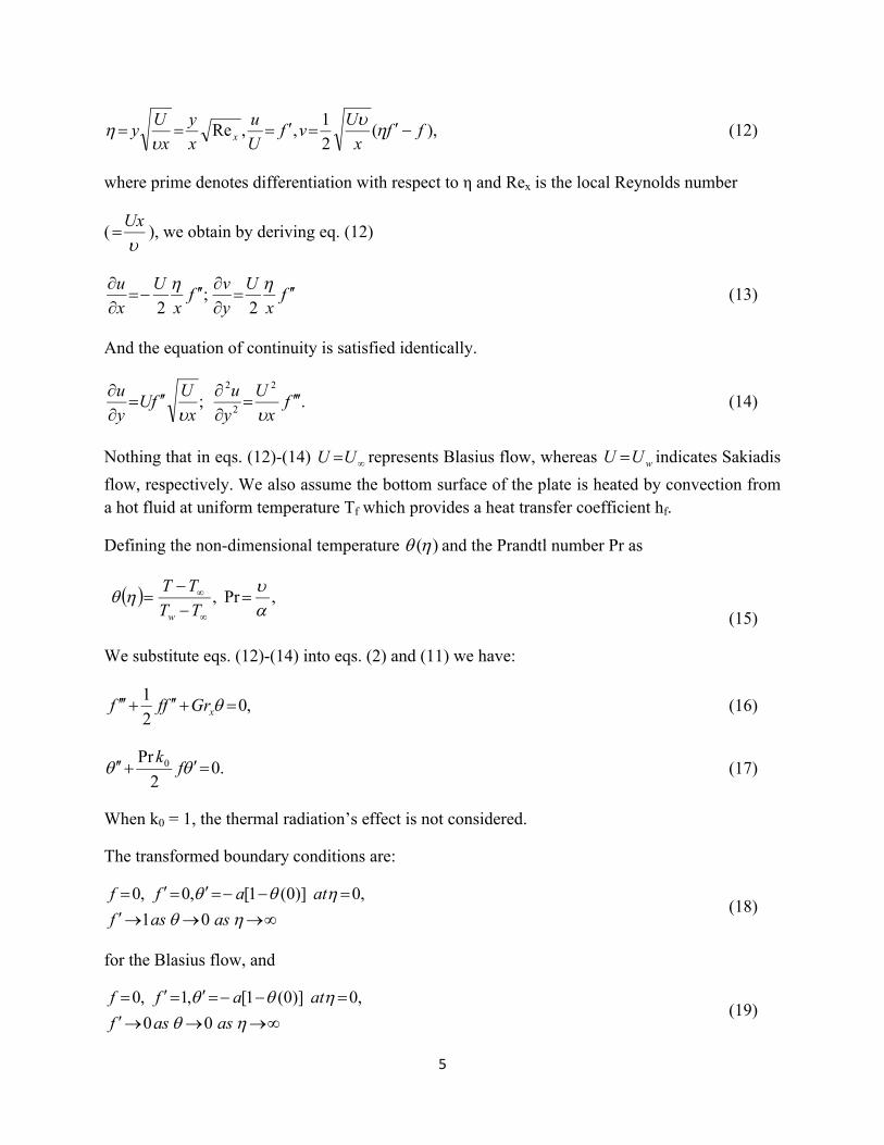
We introduce a similarity variable η and a dimensionless stream function f(η) as

5

),(2

1,,Re ff

x

Uvf

U

u

x

y

x

Uy x

(12)

where prime denotes differentiation with respect to η and Rex is the local Reynolds number

(

Ux ), we obtain by deriving eq. (12)

fx

U

y

vf

x

U

x

u

2;

2(13)

And the equation of continuity is satisfied identically.

.;2

2

2

fx

U

y

u

x

UfU

y

u

(14)

Nothing that in eqs. (12)-(14) UU represents Blasius flow, whereas wUU indicates Sakiadis

flow, respectively. We also assume the bottom surface of the plate is heated by convection from a hot fluid at uniform temperature Tf which provides a heat transfer coefficient hf.

Defining the non-dimensional temperature )( and the Prandtl number Pr as

,Pr,

TT

TT

w (15)

We substitute eqs. (12)-(14) into eqs. (2) and (11) we have:

,02

1 xGrfff (16)

.02

Pr 0 fk

(17)

When k0 = 1, the thermal radiation’s effect is not considered.

The transformed boundary conditions are:

asasf

ataff

01

,0)]0(1[,0,0(18)

for the Blasius flow, and

asasf

ataff

00

,0)]0(1[,1,0(19)

6

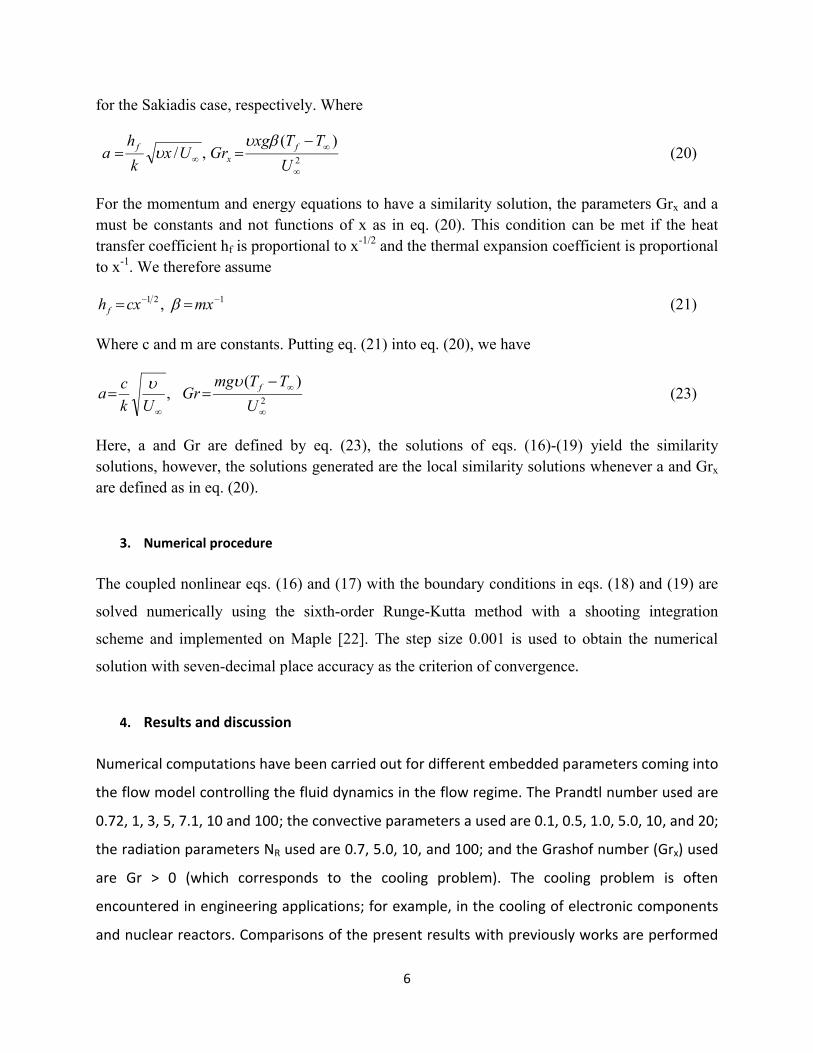
for the Sakiadis case, respectively. Where

2

)(,/

U

TTxgGrUx

k

ha f

xf

(20)

For the momentum and energy equations to have a similarity solution, the parameters Grx and a must be constants and not functions of x as in eq. (20). This condition can be met if the heat transfer coefficient hf is proportional to x-1/2 and the thermal expansion coefficient is proportional to x-1. We therefore assume

121 , mxcxhf (21)

Where c and m are constants. Putting eq. (21) into eq. (20), we have

2

)(,

U

TTmgGr

Uk

ca f

(23)

Here, a and Gr are defined by eq. (23), the solutions of eqs. (16)-(19) yield the similarity solutions, however, the solutions generated are the local similarity solutions whenever a and Grx

are defined as in eq. (20).

3. Numerical procedure

The coupled nonlinear eqs. (16) and (17) with the boundary conditions in eqs. (18) and (19) are

solved numerically using the sixth-order Runge-Kutta method with a shooting integration

scheme and implemented on Maple [22]. The step size 0.001 is used to obtain the numerical

solution with seven-decimal place accuracy as the criterion of convergence.

4. Results and discussion

Numerical computations have been carried out for different embedded parameters coming into

the flow model controlling the fluid dynamics in the flow regime. The Prandtl number used are

0.72, 1, 3, 5, 7.1, 10 and 100; the convective parameters a used are 0.1, 0.5, 1.0, 5.0, 10, and 20;

the radiation parameters NR used are 0.7, 5.0, 10, and 100; and the Grashof number (Grx) used

are Gr > 0 (which corresponds to the cooling problem). The cooling problem is often

encountered in engineering applications; for example, in the cooling of electronic components

and nuclear reactors. Comparisons of the present results with previously works are performed

7

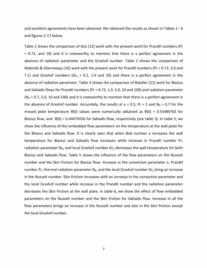
and excellent agreements have been obtained. We obtained the results as shown in Tables 1 - 6

and figures 1-17 below.

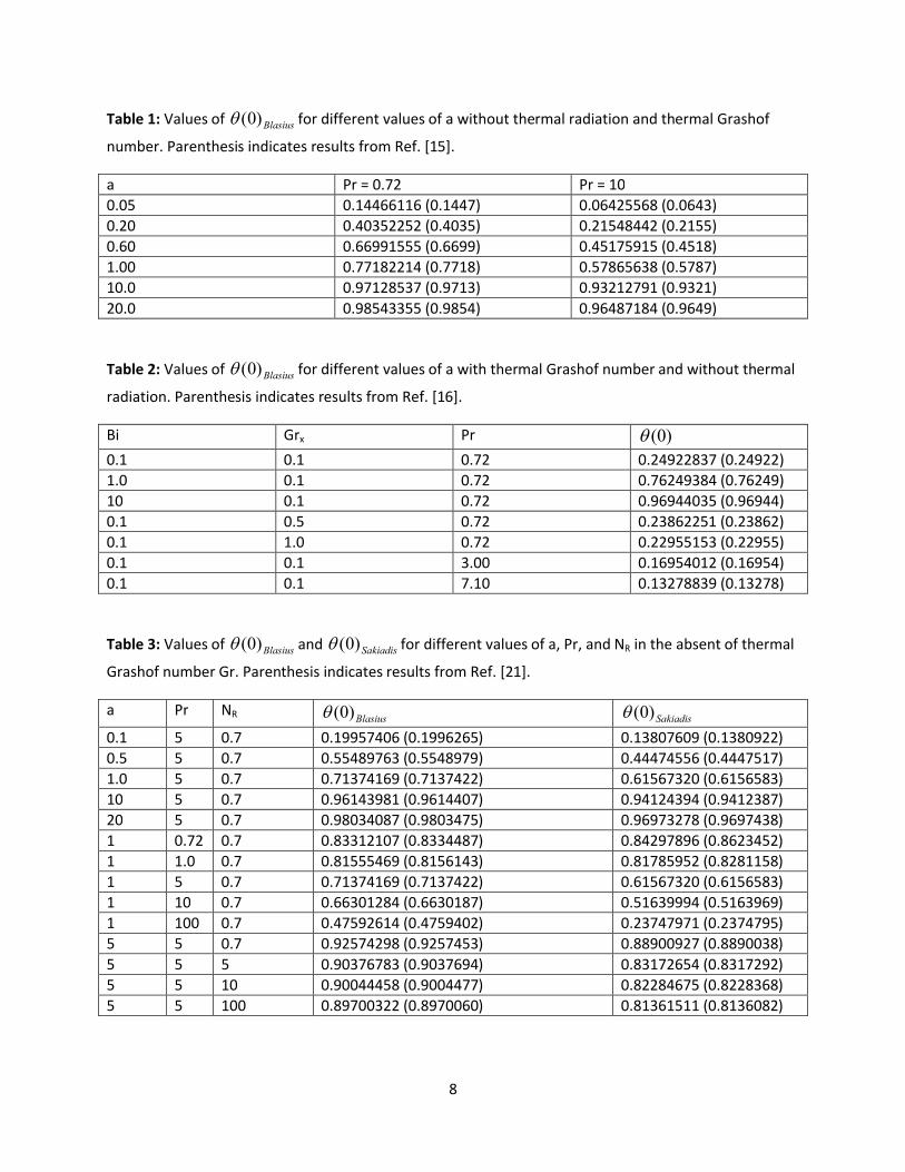
Table 1 shows the comparison of Aziz [15] work with the present work for Prandtl numbers (Pr

= 0.72, and 10) and it is noteworthy to mention that there is a perfect agreement in the

absence of radiation parameter and the Grashof number. Table 2 shows the comparison of

Makinde & Olanrewaju [16] work with the present work for Prandtl numbers (Pr = 0.72, 3.0 and

7.1) and Grashof numbers (Grx = 0.1, 1.0 and 10) and there is a perfect agreement in the

absence of radiation parameter. Table 3 shows the comparison of Bataller [21] work for Blasius

and Sakiadis flows for Prandtl numbers (Pr = 0.72, 1.0, 5.0, 10 and 100) and radiation parameter

(NR = 0.7, 5.0, 10 and 100) and it is noteworthy to mention that there is a perfect agreement in

the absence of Grashof number. Accurately, the results at a = 0.5, Pr = 5 and NR = 0.7 for the

missed plate temperature θ(0) values were numerically obtained as θ(0) = 0.55489763 for

Blasius flow, and θ(0) = 0.44474556 for Sakiadis flow, respectively (see table 3). In table 5, we

show the influence of the embedded flow parameters on the temperature at the wall plate for

the Blasius and Sakiadis flow. It is clearly seen that when Biot number a increases the wall

temperature for Blasius and Sakiadis flow increases while increase in Prandtl number Pr,

radiation parameter NR, and local Grashof number Grx decreases the wall temperature for both

Blasius and Sakiadis flow. Table 5 shows the influence of the flow parameters on the Nusselt

number and the Skin friction for Blasius flow. Increase in the convective parameter a, Prandtl

number Pr, thermal radiation parameter NR, and the local Grashof number Grx bring an increase

in the Nusselt number. Skin friction increases with an increase in the convective parameter and

the local Grashof number while increase in the Prandtl number and the radiation parameter

decreases the Skin friction at the wall plate. In table 6, we show the effect of flow embedded

parameters on the Nusselt number and the Skin friction for Sakiadis flow. Increase in all the

flow parameters brings an increase in the Nusselt number and also in the Skin friction except

the local Grashof number.

8

Table 1: Values of Blasius)0( for different values of a without thermal radiation and thermal Grashof

number. Parenthesis indicates results from Ref. [15].

a Pr = 0.72 Pr = 100.05 0.14466116 (0.1447) 0.06425568 (0.0643)0.20 0.40352252 (0.4035) 0.21548442 (0.2155)0.60 0.66991555 (0.6699) 0.45175915 (0.4518)1.00 0.77182214 (0.7718) 0.57865638 (0.5787)10.0 0.97128537 (0.9713) 0.93212791 (0.9321)20.0 0.98543355 (0.9854) 0.96487184 (0.9649)

Table 2: Values of Blasius)0( for different values of a with thermal Grashof number and without thermal

radiation. Parenthesis indicates results from Ref. [16].

Bi Grx Pr )0(0.1 0.1 0.72 0.24922837 (0.24922)1.0 0.1 0.72 0.76249384 (0.76249)10 0.1 0.72 0.96944035 (0.96944)0.1 0.5 0.72 0.23862251 (0.23862)0.1 1.0 0.72 0.22955153 (0.22955)0.1 0.1 3.00 0.16954012 (0.16954)0.1 0.1 7.10 0.13278839 (0.13278)

Table 3: Values of Blasius)0( and Sakiadis)0( for different values of a, Pr, and NR in the absent of thermal

Grashof number Gr. Parenthesis indicates results from Ref. [21].

a Pr NR Blasius)0( Sakiadis)0(0.1 5 0.7 0.19957406 (0.1996265) 0.13807609 (0.1380922)0.5 5 0.7 0.55489763 (0.5548979) 0.44474556 (0.4447517)1.0 5 0.7 0.71374169 (0.7137422) 0.61567320 (0.6156583)10 5 0.7 0.96143981 (0.9614407) 0.94124394 (0.9412387)20 5 0.7 0.98034087 (0.9803475) 0.96973278 (0.9697438)1 0.72 0.7 0.83312107 (0.8334487) 0.84297896 (0.8623452)1 1.0 0.7 0.81555469 (0.8156143) 0.81785952 (0.8281158)1 5 0.7 0.71374169 (0.7137422) 0.61567320 (0.6156583)1 10 0.7 0.66301284 (0.6630187) 0.51639994 (0.5163969)1 100 0.7 0.47592614 (0.4759402) 0.23747971 (0.2374795)5 5 0.7 0.92574298 (0.9257453) 0.88900927 (0.8890038)5 5 5 0.90376783 (0.9037694) 0.83172654 (0.8317292)5 5 10 0.90044458 (0.9004477) 0.82284675 (0.8228368)5 5 100 0.89700322 (0.8970060) 0.81361511 (0.8136082)

9

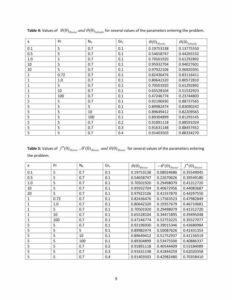
Table 4: Values of SakiadisBlasius and )0()0( for several values of the parameters entering the problem.

a Pr NR Grx Blasius)0( Sakiadis)0(0.1 5 0.7 0.1 0.19753138 0.137755500.5 5 0.7 0.1 0.54658747 0.442655321.0 5 0.7 0.1 0.70501920 0.6129289210 5 0.7 0.1 0.95932704 0.9402760120 5 0.7 0.1 0.97922106 0.969203911 0.72 0.7 0.1 0.82436476 0.831164111 1.0 0.7 0.1 0.80642320 0.805728101 5 0.7 0.1 0.70501920 0.612928921 10 0.7 0.1 0.65528104 0.515329231 100 0.7 0.1 0.47246774 0.237448035 5 0.7 0.1 0.92196930 0.887375655 5 5 0.1 0.89982474 0.830902425 5 10 0.1 0.89649412 0.822095655 5 100 0.1 0.89304899 0.812931455 5 0.7 0.2 0.91891118 0.885910245 5 0.7 0.3 0.91631148 0.884574525 5 0.7 0.4 0.91403503 0.88334270

Table 5: Values of BlasiusBlasiusBlasius andf )0()0(,)0( for several values of the parameters entering

the problem.

a Pr NR Grx Blasius)0( Blasius)0( Blasiusf )0(0.1 5 0.7 0.1 0.19753138 0.08024686 0.355490450.5 5 0.7 0.1 0.54658747 0.22670626 0.395491801.0 5 0.7 0.1 0.70501920 0.29498079 0.4131272010 5 0.7 0.1 0.95932704 0.40672956 0.4408368720 5 0.7 0.1 0.97922106 0.41557870 0.442975501 0.72 0.7 0.1 0.82436476 0.17563523 0.479828491 1.0 0.7 0.1 0.80642320 0.19357679 0.467106811 5 0.7 0.1 0.70501920 0.29498079 0.413127201 10 0.7 0.1 0.65528104 0.34471895 0.394950481 100 0.7 0.1 0.47246774 0.52753225 0.355270775 5 0.7 0.1 0.92196930 0.39015346 0.436809845 5 5 0.1 0.89982474 0.50087626 0.414313535 5 10 0.1 0.89649412 0.51752937 0.411565195 5 100 0.1 0.89304899 0.53475500 0.408863375 5 0.7 0.2 0.91891118 0.40544409 0.531840895 5 0.7 0.3 0.91631148 0.41844259 0.620203585 5 0.7 0.4 0.91403503 0.42982480 0.70358410

10

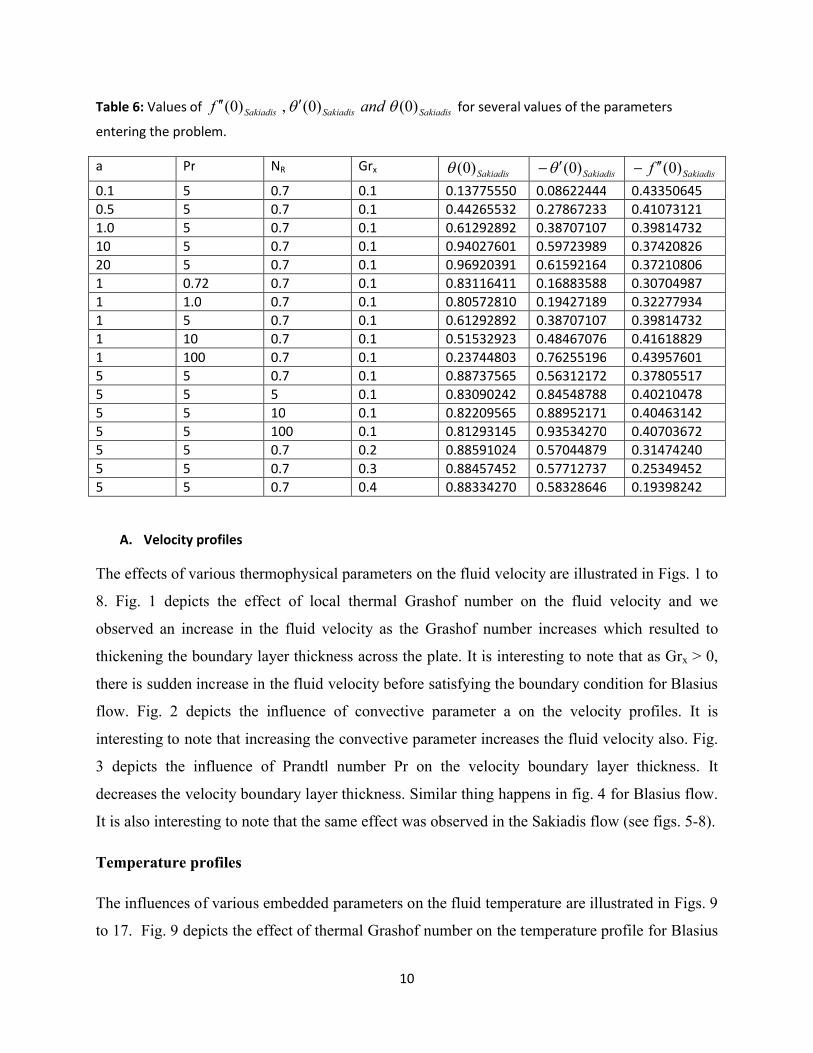
Table 6: Values of SakiadisSakiadisSakiadis andf )0()0(,)0( for several values of the parameters

entering the problem.

a Pr NR Grx Sakiadis)0( Sakiadis)0( Sakiadisf )0(0.1 5 0.7 0.1 0.13775550 0.08622444 0.433506450.5 5 0.7 0.1 0.44265532 0.27867233 0.410731211.0 5 0.7 0.1 0.61292892 0.38707107 0.3981473210 5 0.7 0.1 0.94027601 0.59723989 0.3742082620 5 0.7 0.1 0.96920391 0.61592164 0.372108061 0.72 0.7 0.1 0.83116411 0.16883588 0.307049871 1.0 0.7 0.1 0.80572810 0.19427189 0.322779341 5 0.7 0.1 0.61292892 0.38707107 0.398147321 10 0.7 0.1 0.51532923 0.48467076 0.416188291 100 0.7 0.1 0.23744803 0.76255196 0.439576015 5 0.7 0.1 0.88737565 0.56312172 0.378055175 5 5 0.1 0.83090242 0.84548788 0.402104785 5 10 0.1 0.82209565 0.88952171 0.404631425 5 100 0.1 0.81293145 0.93534270 0.407036725 5 0.7 0.2 0.88591024 0.57044879 0.314742405 5 0.7 0.3 0.88457452 0.57712737 0.253494525 5 0.7 0.4 0.88334270 0.58328646 0.19398242

A. Velocity profiles

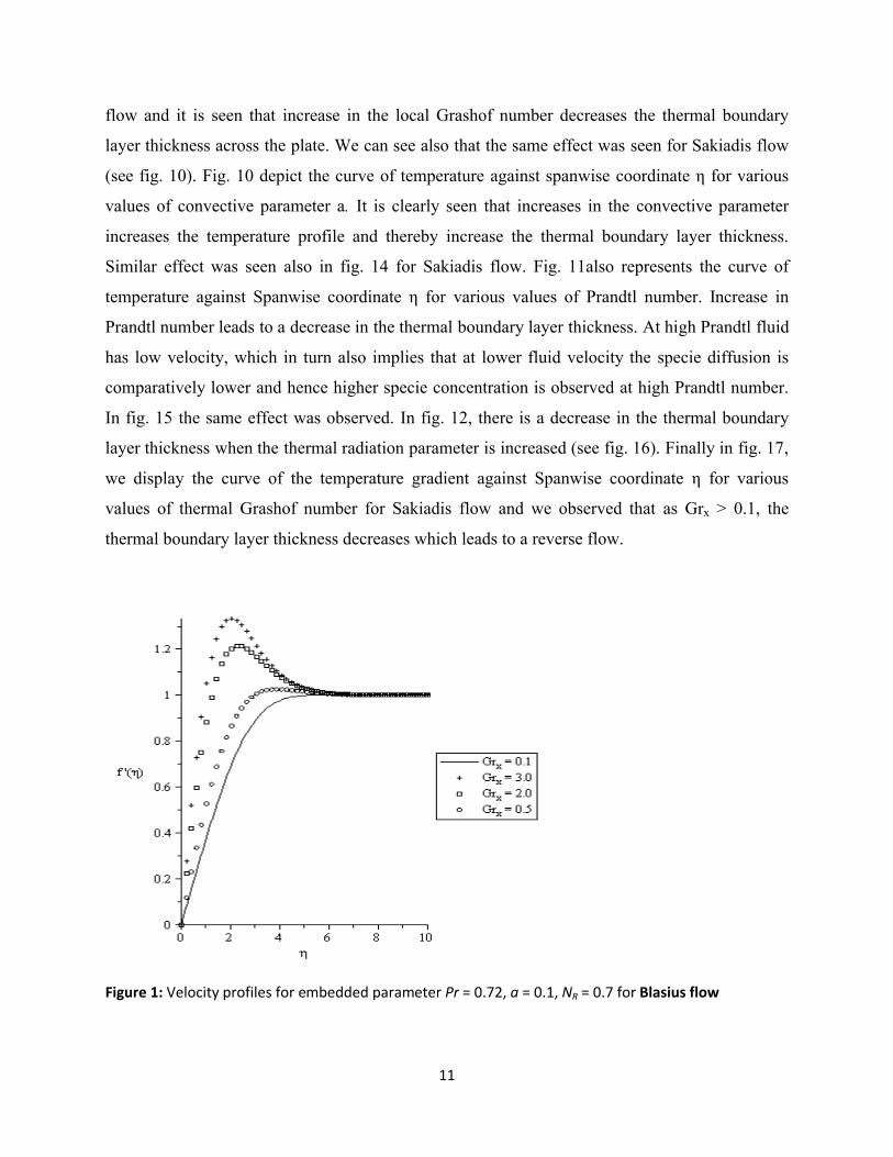
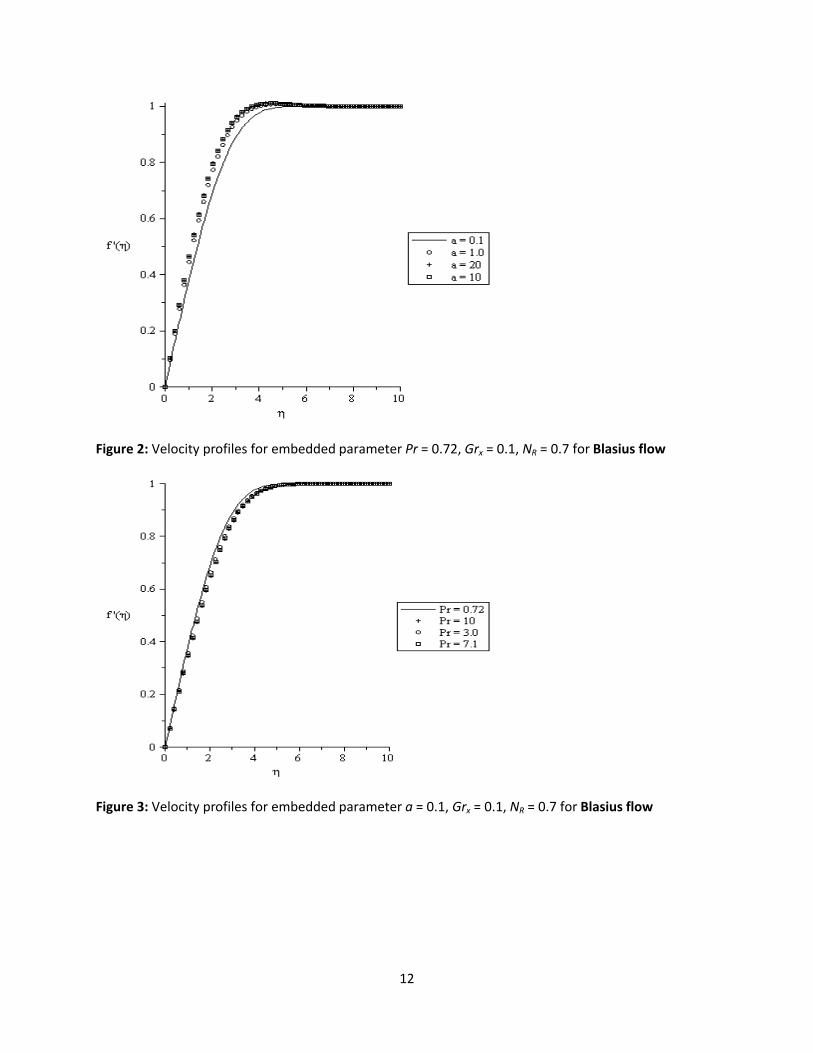
The effects of various thermophysical parameters on the fluid velocity are illustrated in Figs. 1 to

8. Fig. 1 depicts the effect of local thermal Grashof number on the fluid velocity and we

observed an increase in the fluid velocity as the Grashof number increases which resulted to

thickening the boundary layer thickness across the plate. It is interesting to note that as Grx > 0,

there is sudden increase in the fluid velocity before satisfying the boundary condition for Blasius

flow. Fig. 2 depicts the influence of convective parameter a on the velocity profiles. It is

interesting to note that increasing the convective parameter increases the fluid velocity also. Fig.

3 depicts the influence of Prandtl number Pr on the velocity boundary layer thickness. It

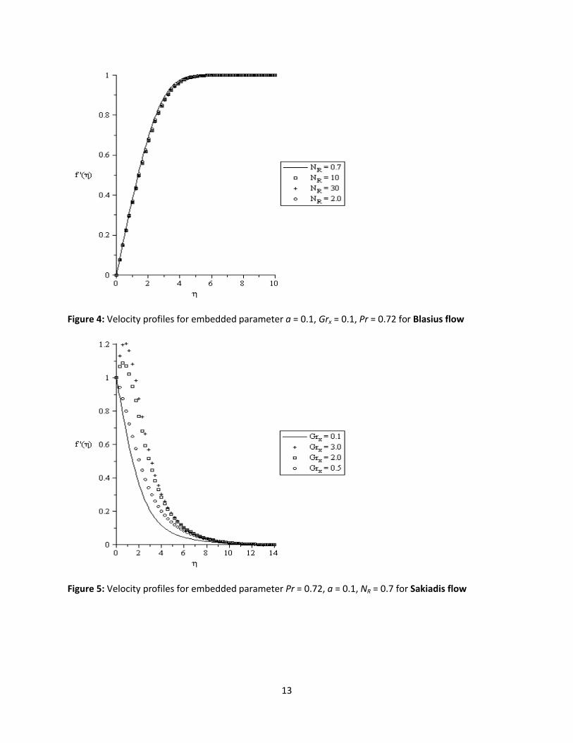
decreases the velocity boundary layer thickness. Similar thing happens in fig. 4 for Blasius flow.

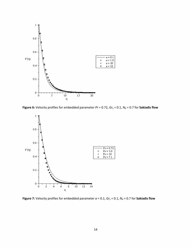
It is also interesting to note that the same effect was observed in the Sakiadis flow (see figs. 5-8).

Temperature profiles

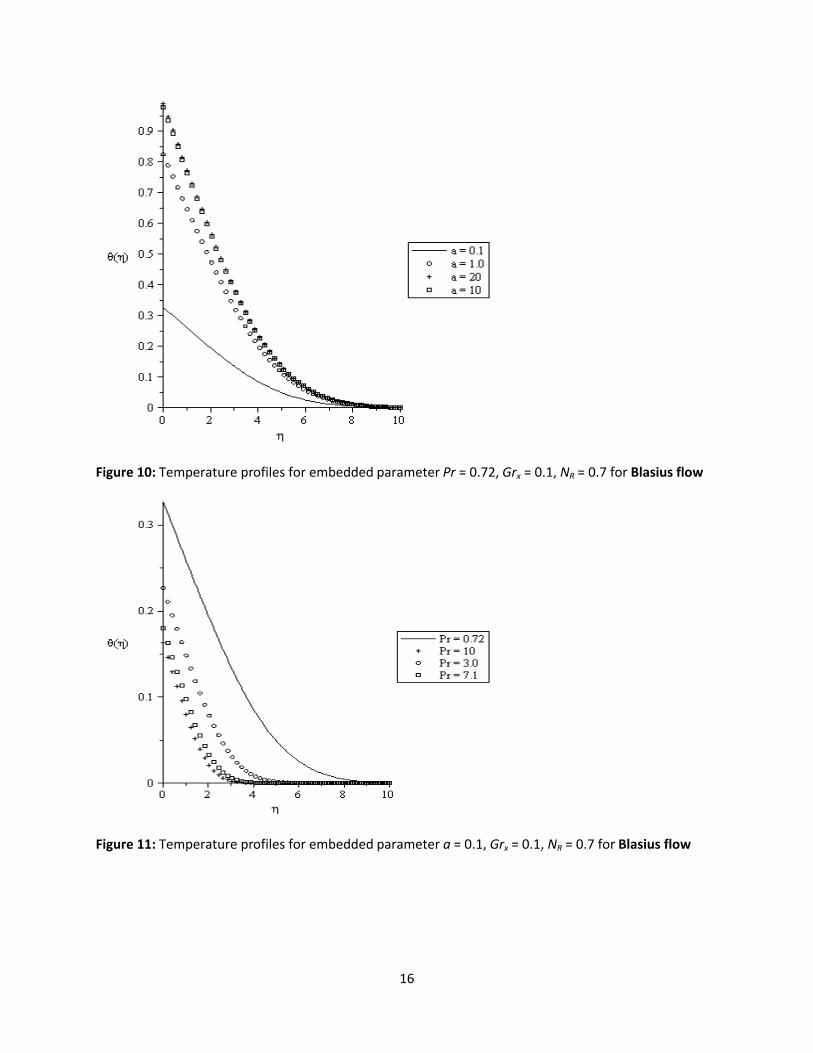
The influences of various embedded parameters on the fluid temperature are illustrated in Figs. 9

to 17. Fig. 9 depicts the effect of thermal Grashof number on the temperature profile for Blasius

11

flow and it is seen that increase in the local Grashof number decreases the thermal boundary

layer thickness across the plate. We can see also that the same effect was seen for Sakiadis flow

(see fig. 10). Fig. 10 depict the curve of temperature against spanwise coordinate η for various

values of convective parameter a. It is clearly seen that increases in the convective parameter

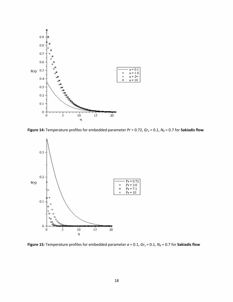
increases the temperature profile and thereby increase the thermal boundary layer thickness.

Similar effect was seen also in fig. 14 for Sakiadis flow. Fig. 11also represents the curve of

temperature against Spanwise coordinate η for various values of Prandtl number. Increase in

Prandtl number leads to a decrease in the thermal boundary layer thickness. At high Prandtl fluid

has low velocity, which in turn also implies that at lower fluid velocity the specie diffusion is

comparatively lower and hence higher specie concentration is observed at high Prandtl number.

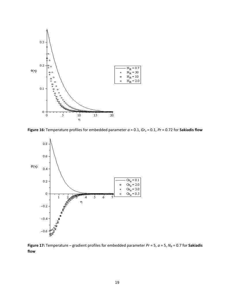
In fig. 15 the same effect was observed. In fig. 12, there is a decrease in the thermal boundary

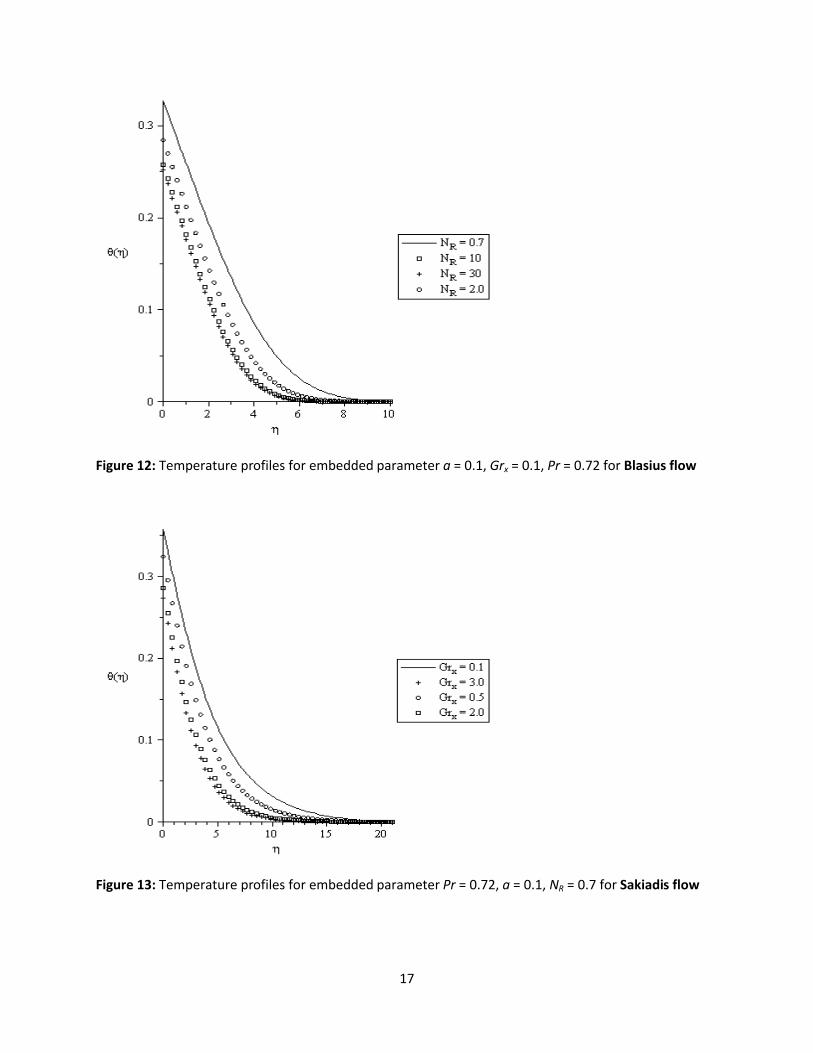
layer thickness when the thermal radiation parameter is increased (see fig. 16). Finally in fig. 17,

we display the curve of the temperature gradient against Spanwise coordinate η for various

values of thermal Grashof number for Sakiadis flow and we observed that as Grx > 0.1, the

thermal boundary layer thickness decreases which leads to a reverse flow.

Figure 1: Velocity profiles for embedded parameter Pr = 0.72, a = 0.1, NR = 0.7 for Blasius flow

12

Figure 2: Velocity profiles for embedded parameter Pr = 0.72, Grx = 0.1, NR = 0.7 for Blasius flow

Figure 3: Velocity profiles for embedded parameter a = 0.1, Grx = 0.1, NR = 0.7 for Blasius flow

13

Figure 4: Velocity profiles for embedded parameter a = 0.1, Grx = 0.1, Pr = 0.72 for Blasius flow

Figure 5: Velocity profiles for embedded parameter Pr = 0.72, a = 0.1, NR = 0.7 for Sakiadis flow

14

Figure 6: Velocity profiles for embedded parameter Pr = 0.72, Grx = 0.1, NR = 0.7 for Sakiadis flow

Figure 7: Velocity profiles for embedded parameter a = 0.1, Grx = 0.1, NR = 0.7 for Sakiadis flow

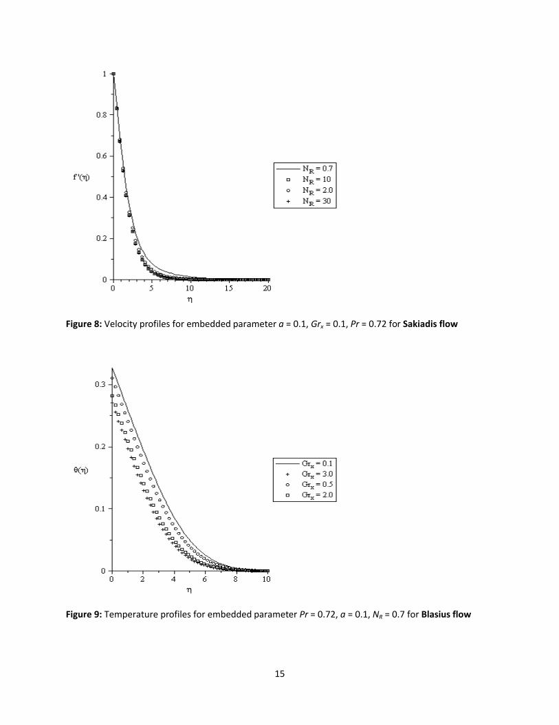
15

Figure 8: Velocity profiles for embedded parameter a = 0.1, Grx = 0.1, Pr = 0.72 for Sakiadis flow

Figure 9: Temperature profiles for embedded parameter Pr = 0.72, a = 0.1, NR = 0.7 for Blasius flow

16

Figure 10: Temperature profiles for embedded parameter Pr = 0.72, Grx = 0.1, NR = 0.7 for Blasius flow

Figure 11: Temperature profiles for embedded parameter a = 0.1, Grx = 0.1, NR = 0.7 for Blasius flow

17

Figure 12: Temperature profiles for embedded parameter a = 0.1, Grx = 0.1, Pr = 0.72 for Blasius flow

Figure 13: Temperature profiles for embedded parameter Pr = 0.72, a = 0.1, NR = 0.7 for Sakiadis flow

18

Figure 14: Temperature profiles for embedded parameter Pr = 0.72, Grx = 0.1, NR = 0.7 for Sakiadis flow

Figure 15: Temperature profiles for embedded parameter a = 0.1, Grx = 0.1, NR = 0.7 for Sakiadis flow

19

Figure 16: Temperature profiles for embedded parameter a = 0.1, Grx = 0.1, Pr = 0.72 for Sakiadis flow

Figure 17: Temperature – gradient profiles for embedded parameter Pr = 5, a = 5, NR = 0.7 for Sakiadis flow

20

5. Conclusions

In this article an IVP procedure is employed to give numerical solutions of the Blasius and Sakiadis momentum, thermal boundary layer over a horizontal flat plate and heat transfer in the presence of thermal radiation and the thermal Grashof number under a convective surface boundary condition. The lower boundary of the plate is at a constant temperature Tf whereas the upper boundary of the surface is maintained at a constant temperature Tw. It is also noted that the temperature of the free stream is assumed as T and also we have Tf > Tw > T . The transformed partial differential equations together

with the boundary conditions are solved numerically by a shooting integration technique alongside with 6th order Runge-Kutta method for better accuracy. Comparisons have been analyzed and the numerical results are listed and graphed. The combined effects of increasing the thermal Grashof number, the Prandtl number and the radiation parameter tend to reduce the thermal boundary layer thickness along the plate which as a result yields a reduction in the fluid temperature. On the contrary, the values of θ(0)Blasius and θ(0)Sakiadis increase with increasing a and decreases with increasing Grx. In general, the Blasius flow gives a thicker thermal boundary layer compared with the Sakiadis flow, but this trend can be reversed at low values of embedded parameters controlling the flow model. Finally, in the limiting

cases, )1.,.( 0 keiNR the thermal radiation influence can be neglected.

Acknowledgements

POO wish to thank the financial support of Covenant University, Ota, Nigeria, West Africa for this research work carried out to promote research output in the Institution.

References

[1] B.C. Sakiadis, Boundary-layer behavior on continuous solid surfaces: I. Boundary-layer equations for

two-dimensional and axisymmetric flow, AIChE J. 7 (1961) 26-28.

[2] F.K. Tsou, E.M. Sparrow, R.J. Glodstein, Flow and heat transfer in the boundary layer on a continuous

moving surface, Int. J. Heat Mass Transfer 10 (1967) 219-235.

[3] L.E. Erickson, L.T. Fan, V.G. Fox, Heat and mass transfer on a moving continuous flat plate with

suction or injection, Ind. Eng. Chem. 5 (1966) 19-25.

[4] L.J. Crane, Flow past a stretching plate, Z. Angew. Math. Phys. (ZAMP) 21 (1970) 645-647.

[5] T. Fang, Further study on a moving-wall boundary-layer problem with mass transfer, Acta Mech. 163

(2003) 183-188.

[6] T. Fang, Similarity solutions for a moving-flat plate thermal boundary layer, Acta Mech. 163 (2003)

161-172.

[7] T. Fang, Influences of fluid property variation on the boundary layers of a stretching surface, Acta

Mech. 171 (2004) 105-118.

[8] T. Fang, Flow over a stretchable disk, Phys. Fluids 19 (2004) 128105.

21

[9] T. Fang, C.F. Lee, A moving-wall boundary layer flow of a slightly rarefied gas free stream over a

moving flat plate, Appl. Math. Lett. 18 (2005) 487-495.

[10] H. Blasius, Grenzschichten in Flussigkeiten mit kleiner reibung, z. math. Phys. 56 (1908) 1-37.

[11] H. Weyl, On the differential equations of the simplest boundary-layer problem, Ann. Math. 43

(1942) 381-407.

[12] E. Magyari, The moving plate thermometer, Int. J. Therm. Sci. 47 (2008) 1436-1441.

[13] R. Cortell, Numerical solutions of the classical Blasius flat-plate problem, Appl. Math. Comput. 170

(2005) 706-710.

[14] J. H. He, A simple perturbation approach to Blasius equation, Appl. Math. Comput. 140 (2003) 217-

222.

[15] A. Aziz, A similarity solution for laminar thermal boundary layer over a flat plate with a convective

surface boundary condition, Commum Nonlinear Sci Numer Simulat 14 (2009) 1064-1068.

[16]. Makinde O. D., Olanrewaju P. O. 2010, “Buoyancy effects on thermal boundary layer over a vertical

plate with a convective surface boundary condition,” Transactions ASME Journal

of Fluids Engineering, Vol. 132, 044502(1-4).

[17] P.O. Olanrewaju, Makinde O.D., Combined effects of internal heat generation and buoyancy force

on boundary layer over a vertical plate with a convective surface boundary condition, Canadian Journal

of Chemical Engineering(To appear).

[18] M.A. Hossain, H.S. Takhar, Radiation effects on mixed convection along a vertical plate with uniform

surface temperature, Heat Mass Transfer 31 (1996) 243-248.

[19] M.A. Hossain, M.A. Alim, D. Rees, The effect of radiation on free convection from a porous vertical

plate, Int. J. Heat Mass Transfer 42 (1999) 181-191.

[20] M.A. Hossain, K. Khanafer, K. Vafai, The effect of radiation on free convection flow of fluid with

variable viscosity from a porous vertical plate, Int. J. Thermal Sci. 40 (2001) 115-124.

[21] R.C. Bataller, Radiation effects for the Blasius and Sakiadis flows with a convective surface boundary

condition, Applied Mathematics and Computation 206 (2008) 832-840.

[22] A. Heck, Introduction to Maple, 3rd Edition, Springer-Verlag, (2003).